Introduction to Statistical Data Analysis
128
Introduction to Statistical Data Analysis James V. Lambers August 15, 2016
Transcript of Introduction to Statistical Data Analysis
Introduction to Statistical Data Analysis
James V. Lambers
August 15, 2016

ii

Contents
1 Working with Data Sets 1
1.1 Introduction . . . . . . . . . . . . . . . . . . . . . . . . . . . . . . . . . . . . . . . 1
1.2 Statistical Software: The R Project . . . . . . . . . . . . . . . . . . . . . . . . . . 1
1.3 Types of Statistics . . . . . . . . . . . . . . . . . . . . . . . . . . . . . . . . . . . 1
1.3.1 Descriptive Statistics . . . . . . . . . . . . . . . . . . . . . . . . . . . . . . 1
1.3.2 Inferential Statistics . . . . . . . . . . . . . . . . . . . . . . . . . . . . . . 2
1.3.3 Ethics in Statistics . . . . . . . . . . . . . . . . . . . . . . . . . . . . . . . 2
1.4 Data Collection and Usage . . . . . . . . . . . . . . . . . . . . . . . . . . . . . . . 4
1.4.1 Data Sources . . . . . . . . . . . . . . . . . . . . . . . . . . . . . . . . . . 4
1.4.2 Levels of Measurement Scales . . . . . . . . . . . . . . . . . . . . . . . . . 5
1.5 Data Display . . . . . . . . . . . . . . . . . . . . . . . . . . . . . . . . . . . . . . 6
1.5.1 Frequency Distributions . . . . . . . . . . . . . . . . . . . . . . . . . . . . 6
1.5.2 Stem and Leaf Displays . . . . . . . . . . . . . . . . . . . . . . . . . . . . 8
1.5.3 Charts . . . . . . . . . . . . . . . . . . . . . . . . . . . . . . . . . . . . . . 9
1.6 Measures of Central Tendency . . . . . . . . . . . . . . . . . . . . . . . . . . . . . 10
1.6.1 Mean . . . . . . . . . . . . . . . . . . . . . . . . . . . . . . . . . . . . . . 11
1.6.2 Median . . . . . . . . . . . . . . . . . . . . . . . . . . . . . . . . . . . . . 12
1.6.3 Mode . . . . . . . . . . . . . . . . . . . . . . . . . . . . . . . . . . . . . . 13
1.6.4 Choosing a Measure . . . . . . . . . . . . . . . . . . . . . . . . . . . . . . 13
1.7 Measures of Dispersion . . . . . . . . . . . . . . . . . . . . . . . . . . . . . . . . . 13
1.7.1 Range . . . . . . . . . . . . . . . . . . . . . . . . . . . . . . . . . . . . . . 13
1.7.2 Variance . . . . . . . . . . . . . . . . . . . . . . . . . . . . . . . . . . . . . 14
1.7.3 Standard Deviation . . . . . . . . . . . . . . . . . . . . . . . . . . . . . . 14
1.7.4 Quartiles . . . . . . . . . . . . . . . . . . . . . . . . . . . . . . . . . . . . 15
1.8 Exercises . . . . . . . . . . . . . . . . . . . . . . . . . . . . . . . . . . . . . . . . 16
2 Probability 23
2.1 Introduction . . . . . . . . . . . . . . . . . . . . . . . . . . . . . . . . . . . . . . . 23
2.1.1 Events . . . . . . . . . . . . . . . . . . . . . . . . . . . . . . . . . . . . . . 23
2.1.2 Types of Probability . . . . . . . . . . . . . . . . . . . . . . . . . . . . . . 23
2.1.3 Properties of Probability . . . . . . . . . . . . . . . . . . . . . . . . . . . . 24
2.2 Conditional Probability . . . . . . . . . . . . . . . . . . . . . . . . . . . . . . . . 25
2.3 Independent Events . . . . . . . . . . . . . . . . . . . . . . . . . . . . . . . . . . 25
2.4 Intersection of Events . . . . . . . . . . . . . . . . . . . . . . . . . . . . . . . . . 26
iii

iv CONTENTS
2.4.1 Multiplication Rule . . . . . . . . . . . . . . . . . . . . . . . . . . . . . . . 26
2.4.2 Mutually Exclusive Events . . . . . . . . . . . . . . . . . . . . . . . . . . 27
2.5 Union of Events . . . . . . . . . . . . . . . . . . . . . . . . . . . . . . . . . . . . . 28
2.5.1 Addition Rule . . . . . . . . . . . . . . . . . . . . . . . . . . . . . . . . . . 28
2.6 Bayes’ Theorem . . . . . . . . . . . . . . . . . . . . . . . . . . . . . . . . . . . . . 28
2.7 Counting Principles . . . . . . . . . . . . . . . . . . . . . . . . . . . . . . . . . . 29
2.7.1 The Fundamental Counting Principle . . . . . . . . . . . . . . . . . . . . 29
2.7.2 Permutations . . . . . . . . . . . . . . . . . . . . . . . . . . . . . . . . . . 30
2.7.3 Combinations . . . . . . . . . . . . . . . . . . . . . . . . . . . . . . . . . . 31
2.7.4 Permutations and Combinations in R . . . . . . . . . . . . . . . . . . . . 31
2.8 Exercises . . . . . . . . . . . . . . . . . . . . . . . . . . . . . . . . . . . . . . . . 31
3 Probability Distributions 37
3.1 Introduction . . . . . . . . . . . . . . . . . . . . . . . . . . . . . . . . . . . . . . . 37
3.1.1 Random Variables . . . . . . . . . . . . . . . . . . . . . . . . . . . . . . . 37
3.1.2 Discrete Probability Distributions . . . . . . . . . . . . . . . . . . . . . . 37
3.1.3 Rules for Discrete Distributions . . . . . . . . . . . . . . . . . . . . . . . . 38
3.1.4 Mean . . . . . . . . . . . . . . . . . . . . . . . . . . . . . . . . . . . . . . 38
3.1.5 Variance and Standard Deviation . . . . . . . . . . . . . . . . . . . . . . . 39
3.2 Uniform Distribution . . . . . . . . . . . . . . . . . . . . . . . . . . . . . . . . . . 39
3.3 Binomial Distribution . . . . . . . . . . . . . . . . . . . . . . . . . . . . . . . . . 39
3.3.1 Binomial Experiments . . . . . . . . . . . . . . . . . . . . . . . . . . . . . 39
3.3.2 The Binomial Distribution . . . . . . . . . . . . . . . . . . . . . . . . . . . 40
3.3.3 The Mean and Standard Deviation . . . . . . . . . . . . . . . . . . . . . . 41
3.4 Hypergeometric Distribution . . . . . . . . . . . . . . . . . . . . . . . . . . . . . 41
3.5 Poisson Distribution . . . . . . . . . . . . . . . . . . . . . . . . . . . . . . . . . . 42
3.5.1 Poisson Processes . . . . . . . . . . . . . . . . . . . . . . . . . . . . . . . . 42
3.5.2 The Poisson Distribution . . . . . . . . . . . . . . . . . . . . . . . . . . . 43
3.5.3 Approximating the Binomial Distribution . . . . . . . . . . . . . . . . . . 44
3.6 Continuous Distributions . . . . . . . . . . . . . . . . . . . . . . . . . . . . . . . 45
3.7 Continuous Uniform Distribution . . . . . . . . . . . . . . . . . . . . . . . . . . . 45
3.8 Exponential Distribution . . . . . . . . . . . . . . . . . . . . . . . . . . . . . . . . 46
3.9 Normal Distribution . . . . . . . . . . . . . . . . . . . . . . . . . . . . . . . . . . 46
3.9.1 Characteristics . . . . . . . . . . . . . . . . . . . . . . . . . . . . . . . . . 47
3.9.2 Calculating Probabilities . . . . . . . . . . . . . . . . . . . . . . . . . . . . 48
3.9.3 Approximating the Binomial Distribution . . . . . . . . . . . . . . . . . . 49
3.10 Exercises . . . . . . . . . . . . . . . . . . . . . . . . . . . . . . . . . . . . . . . . 49
4 Sampling 55
4.1 Introduction . . . . . . . . . . . . . . . . . . . . . . . . . . . . . . . . . . . . . . . 55
4.2 Methods of Sampling . . . . . . . . . . . . . . . . . . . . . . . . . . . . . . . . . . 55
4.2.1 Simple Sampling . . . . . . . . . . . . . . . . . . . . . . . . . . . . . . . . 55
4.2.2 Systematic Sampling . . . . . . . . . . . . . . . . . . . . . . . . . . . . . . 55
4.2.3 Cluster Sampling . . . . . . . . . . . . . . . . . . . . . . . . . . . . . . . . 56
4.2.4 Stratified Sampling . . . . . . . . . . . . . . . . . . . . . . . . . . . . . . . 56

CONTENTS v
4.3 Sampling Pitfalls . . . . . . . . . . . . . . . . . . . . . . . . . . . . . . . . . . . . 56
4.3.1 Sampling Errors . . . . . . . . . . . . . . . . . . . . . . . . . . . . . . . . 56
4.3.2 Poor Sampling Technique . . . . . . . . . . . . . . . . . . . . . . . . . . . 56
4.4 Sampling Distributions . . . . . . . . . . . . . . . . . . . . . . . . . . . . . . . . . 56
4.4.1 Sampling Distribution of the Mean . . . . . . . . . . . . . . . . . . . . . . 57
4.5 The Central Limit Theorem . . . . . . . . . . . . . . . . . . . . . . . . . . . . . . 58
4.5.1 Standard Error . . . . . . . . . . . . . . . . . . . . . . . . . . . . . . . . . 58
4.6 Sampling Distribution of the Proportion . . . . . . . . . . . . . . . . . . . . . . . 59
4.7 Exercises . . . . . . . . . . . . . . . . . . . . . . . . . . . . . . . . . . . . . . . . 60
5 Confidence Intervals 63
5.1 Introduction . . . . . . . . . . . . . . . . . . . . . . . . . . . . . . . . . . . . . . . 63
5.2 Confidence Intervals for Means . . . . . . . . . . . . . . . . . . . . . . . . . . . . 63
5.2.1 Large Samples . . . . . . . . . . . . . . . . . . . . . . . . . . . . . . . . . 63
5.2.2 Small Samples . . . . . . . . . . . . . . . . . . . . . . . . . . . . . . . . . 66
5.3 Confidence Intervals for Proportions . . . . . . . . . . . . . . . . . . . . . . . . . 67
5.3.1 Calculating Confidence Intervals . . . . . . . . . . . . . . . . . . . . . . . 67
5.3.2 Determining the Sample Size . . . . . . . . . . . . . . . . . . . . . . . . . 68
5.4 Exercises . . . . . . . . . . . . . . . . . . . . . . . . . . . . . . . . . . . . . . . . 68
6 Hypothesis Testing 71
6.1 Introduction . . . . . . . . . . . . . . . . . . . . . . . . . . . . . . . . . . . . . . . 71
6.1.1 The Null and Alternative Hypotheses . . . . . . . . . . . . . . . . . . . . 71
6.1.2 Stating the Null and Alternative Hypotheses . . . . . . . . . . . . . . . . 71
6.2 Type I and Type II Errors . . . . . . . . . . . . . . . . . . . . . . . . . . . . . . . 72
6.3 Two-Tail Hypothesis Testing . . . . . . . . . . . . . . . . . . . . . . . . . . . . . 72
6.4 One-Tail Hypothesis Testing . . . . . . . . . . . . . . . . . . . . . . . . . . . . . . 73
6.5 Hypothesis Testing with One Sample . . . . . . . . . . . . . . . . . . . . . . . . . 73
6.5.1 Testing for the Mean, Large Sample . . . . . . . . . . . . . . . . . . . . . 73
6.5.2 The Role of α . . . . . . . . . . . . . . . . . . . . . . . . . . . . . . . . . . 75
6.5.3 p-Values . . . . . . . . . . . . . . . . . . . . . . . . . . . . . . . . . . . . . 75
6.5.4 Testing for the Mean, Small Sample . . . . . . . . . . . . . . . . . . . . . 76
6.5.5 Testing for the Proportion, Large Samples . . . . . . . . . . . . . . . . . . 77
6.5.6 Writing Functions in R . . . . . . . . . . . . . . . . . . . . . . . . . . . . 78
6.6 Hypothesis Testing with Two Samples . . . . . . . . . . . . . . . . . . . . . . . . 79
6.6.1 Sampling Distribution for the Difference of Means . . . . . . . . . . . . . 79
6.6.2 Testing for Difference of Means, Large Samples . . . . . . . . . . . . . . . 80
6.6.3 Testing for Difference of Means, Unknown Variance . . . . . . . . . . . . 80
6.6.4 Testing for Difference of Proportions . . . . . . . . . . . . . . . . . . . . . 82
6.7 Summary . . . . . . . . . . . . . . . . . . . . . . . . . . . . . . . . . . . . . . . . 83
6.8 Exercises . . . . . . . . . . . . . . . . . . . . . . . . . . . . . . . . . . . . . . . . 84
vi CONTENTS
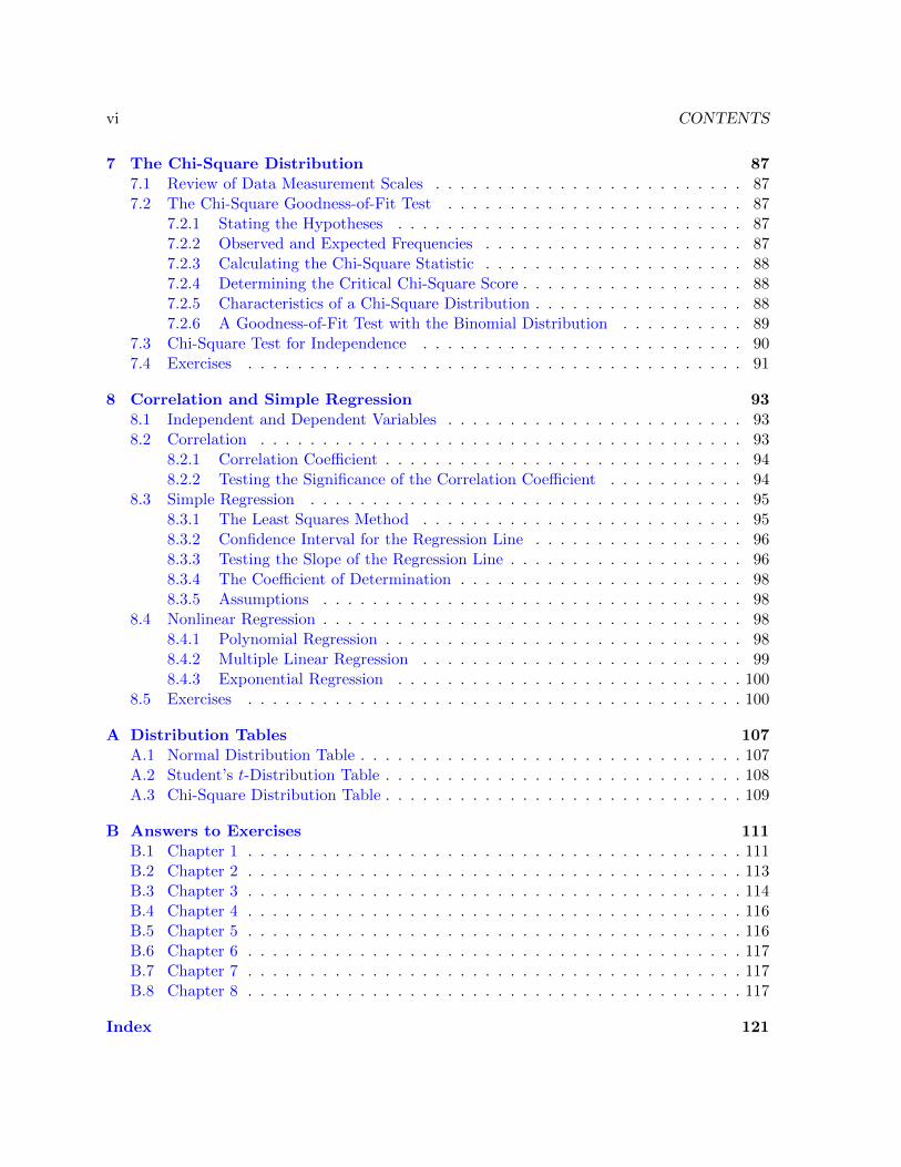
7 The Chi-Square Distribution 877.1 Review of Data Measurement Scales . . . . . . . . . . . . . . . . . . . . . . . . . 877.2 The Chi-Square Goodness-of-Fit Test . . . . . . . . . . . . . . . . . . . . . . . . 87
7.2.1 Stating the Hypotheses . . . . . . . . . . . . . . . . . . . . . . . . . . . . 877.2.2 Observed and Expected Frequencies . . . . . . . . . . . . . . . . . . . . . 877.2.3 Calculating the Chi-Square Statistic . . . . . . . . . . . . . . . . . . . . . 887.2.4 Determining the Critical Chi-Square Score . . . . . . . . . . . . . . . . . . 887.2.5 Characteristics of a Chi-Square Distribution . . . . . . . . . . . . . . . . . 887.2.6 A Goodness-of-Fit Test with the Binomial Distribution . . . . . . . . . . 89
7.3 Chi-Square Test for Independence . . . . . . . . . . . . . . . . . . . . . . . . . . 907.4 Exercises . . . . . . . . . . . . . . . . . . . . . . . . . . . . . . . . . . . . . . . . 91
8 Correlation and Simple Regression 938.1 Independent and Dependent Variables . . . . . . . . . . . . . . . . . . . . . . . . 938.2 Correlation . . . . . . . . . . . . . . . . . . . . . . . . . . . . . . . . . . . . . . . 93
8.2.1 Correlation Coefficient . . . . . . . . . . . . . . . . . . . . . . . . . . . . . 948.2.2 Testing the Significance of the Correlation Coefficient . . . . . . . . . . . 94
8.3 Simple Regression . . . . . . . . . . . . . . . . . . . . . . . . . . . . . . . . . . . 958.3.1 The Least Squares Method . . . . . . . . . . . . . . . . . . . . . . . . . . 958.3.2 Confidence Interval for the Regression Line . . . . . . . . . . . . . . . . . 968.3.3 Testing the Slope of the Regression Line . . . . . . . . . . . . . . . . . . . 968.3.4 The Coefficient of Determination . . . . . . . . . . . . . . . . . . . . . . . 988.3.5 Assumptions . . . . . . . . . . . . . . . . . . . . . . . . . . . . . . . . . . 98
8.4 Nonlinear Regression . . . . . . . . . . . . . . . . . . . . . . . . . . . . . . . . . . 988.4.1 Polynomial Regression . . . . . . . . . . . . . . . . . . . . . . . . . . . . . 988.4.2 Multiple Linear Regression . . . . . . . . . . . . . . . . . . . . . . . . . . 998.4.3 Exponential Regression . . . . . . . . . . . . . . . . . . . . . . . . . . . . 100
8.5 Exercises . . . . . . . . . . . . . . . . . . . . . . . . . . . . . . . . . . . . . . . . 100
A Distribution Tables 107A.1 Normal Distribution Table . . . . . . . . . . . . . . . . . . . . . . . . . . . . . . . 107A.2 Student’s t-Distribution Table . . . . . . . . . . . . . . . . . . . . . . . . . . . . . 108A.3 Chi-Square Distribution Table . . . . . . . . . . . . . . . . . . . . . . . . . . . . . 109
B Answers to Exercises 111B.1 Chapter 1 . . . . . . . . . . . . . . . . . . . . . . . . . . . . . . . . . . . . . . . . 111B.2 Chapter 2 . . . . . . . . . . . . . . . . . . . . . . . . . . . . . . . . . . . . . . . . 113B.3 Chapter 3 . . . . . . . . . . . . . . . . . . . . . . . . . . . . . . . . . . . . . . . . 114B.4 Chapter 4 . . . . . . . . . . . . . . . . . . . . . . . . . . . . . . . . . . . . . . . . 116B.5 Chapter 5 . . . . . . . . . . . . . . . . . . . . . . . . . . . . . . . . . . . . . . . . 116B.6 Chapter 6 . . . . . . . . . . . . . . . . . . . . . . . . . . . . . . . . . . . . . . . . 117B.7 Chapter 7 . . . . . . . . . . . . . . . . . . . . . . . . . . . . . . . . . . . . . . . . 117B.8 Chapter 8 . . . . . . . . . . . . . . . . . . . . . . . . . . . . . . . . . . . . . . . . 117
Index 121

Chapter 1
Working with Data Sets
1.1 Introduction
This course is an introduction to statistical data analysis. The purpose of the course is toacquaint students with fundamental techniques for gathering data, describing data sets, andmost importantly, making conclusions based on data. Topics that will be covered include prob-ability, probability distributions, sampling, confidence intervals, hypothesis testing, correlation,and regression.
1.2 Statistical Software: The R Project
To illustrate and work with concepts and techniques presented in this course, we will use asoftware tool known as R, which provides a programming environment for statistical computingand graphics. It is freely available for download from the site
http://www.r-project.org/
Throughout these notes, as concepts are presented, relevant R functions and sample code willbe given.
1.3 Types of Statistics
There are two main branches of statistics, descriptive statistics and inferential statistics.
1.3.1 Descriptive Statistics
The purpose of descriptive statistics to summarize and display data in such a way that it canreadily be interpreted. Examples of descriptive statistics are as follows:
• The average, or mean is a convenient way of describing a set of many numbers with justa single number.
• A chart is useful for organizing and summarizing data in meaningful ways.
1
2 CHAPTER 1. WORKING WITH DATA SETS
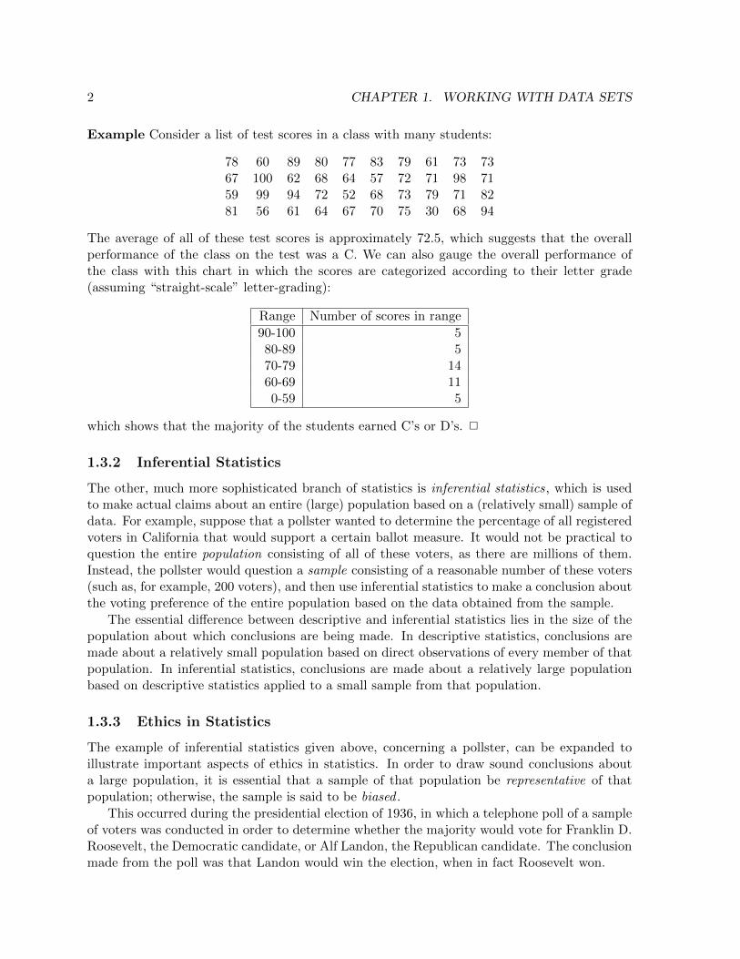
Example Consider a list of test scores in a class with many students:
78 60 89 80 77 83 79 61 73 7367 100 62 68 64 57 72 71 98 7159 99 94 72 52 68 73 79 71 8281 56 61 64 67 70 75 30 68 94
The average of all of these test scores is approximately 72.5, which suggests that the overallperformance of the class on the test was a C. We can also gauge the overall performance ofthe class with this chart in which the scores are categorized according to their letter grade(assuming “straight-scale” letter-grading):
Range Number of scores in range
90-100 580-89 570-79 1460-69 110-59 5
which shows that the majority of the students earned C’s or D’s. 2
1.3.2 Inferential Statistics
The other, much more sophisticated branch of statistics is inferential statistics, which is usedto make actual claims about an entire (large) population based on a (relatively small) sample ofdata. For example, suppose that a pollster wanted to determine the percentage of all registeredvoters in California that would support a certain ballot measure. It would not be practical toquestion the entire population consisting of all of these voters, as there are millions of them.Instead, the pollster would question a sample consisting of a reasonable number of these voters(such as, for example, 200 voters), and then use inferential statistics to make a conclusion aboutthe voting preference of the entire population based on the data obtained from the sample.
The essential difference between descriptive and inferential statistics lies in the size of thepopulation about which conclusions are being made. In descriptive statistics, conclusions aremade about a relatively small population based on direct observations of every member of thatpopulation. In inferential statistics, conclusions are made about a relatively large populationbased on descriptive statistics applied to a small sample from that population.
1.3.3 Ethics in Statistics
The example of inferential statistics given above, concerning a pollster, can be expanded toillustrate important aspects of ethics in statistics. In order to draw sound conclusions abouta large population, it is essential that a sample of that population be representative of thatpopulation; otherwise, the sample is said to be biased .
This occurred during the presidential election of 1936, in which a telephone poll of a sampleof voters was conducted in order to determine whether the majority would vote for Franklin D.Roosevelt, the Democratic candidate, or Alf Landon, the Republican candidate. The conclusionmade from the poll was that Landon would win the election, when in fact Roosevelt won.

1.3. TYPES OF STATISTICS 3
The reason why the poll yielded an incorrect conclusion was that it was conducted bytelephone, and in 1936, telephones existed primarily in more affluent households, which tendedto vote Republican. That is, the method of polling led to an unintentional bias. In some cases,unfortunately, a sample can be biased intentionally, in order to make a false conclusion thatsupports one’s agenda.
Just as telephone polling was problematic decades ago, internet polling is problematic today.It is very difficult to ensure that voters in an internet poll vote only once, and it is impossibleto ensure that those who vote are actually representative of any given population. For thisreason, such polls are generally labeled as “unscientific”, although this disclaimer is not alwaysnoted by those who read the results of such polls.
Another example of questionable or unethical uses of statistics is the tactic of emphasizingdifferences through display. Suppose that over a period of three years, the average price of ahome in a certain city has increased from $380,000 to $390,000 to $400,000. Figure 1.1 showstwo charts that display this data, but do so in different ways to either emphasize or de-emphasizethe increase.
Figure 1.1: Different approaches to displaying the same increase in home prices over a three-yearperiod
Note that both charts display exactly the same data, but whereas the chart on the left usesa vertical scale that has the effect of making the yearly increase seem negligible, the chart onthe right uses a vertical scale that makes this same increase seem much more dramatic. Peoplewho report statistics can, unfortunately, use tactics like this to subtly influence consumers ofthe information that they provide.

4 CHAPTER 1. WORKING WITH DATA SETS
1.4 Data Collection and Usage
In this section, we discuss various approaches to data collection, and the ramifications of each.It is important to consider both the source of the data, and the method of measurement usedduring its collection. First, we give some definitions.
• data (singular datum) are values assigned to observations that are made about a popula-tion.
• A parameter is a type of data that describes a characteristic of a population, such as theincome level of every member of the labor force within a city.
• By contrast, a statistic is data that describes a characteristic of a sample, such as thefavorite candy bar of every member of a focus group.
• Information is data transformed into useful facts, typically through inferential statistics.
Example Suppose that a large corporation, that has hundreds of stores throughout the UnitedStates, wants to determine the trend of its sales from year to year. The average revenue of all ofits stores would be considered a parameter, where the population consists of all stores. However,the corporation could consider just a sample of its stores and compute the average revenue forthis subset, which would be a statistic. Suppose that this average is found to be dropping fromyear to year. From this data, the corporation could glean the essential information that it is indanger of going bankrupt if this trend continues, and must act before it is too late. 2
1.4.1 Data Sources
We now examine various sources of data. Regardless of the type of source, data can be catego-rized as either primary data, which is data collected by an individual or organization for theirown use, as opposed to secondary data, which is data collected by others (such as a governmentagency). Regardless of whether one collects their own data or obtains it from elsewhere, itis essential to ensure that this data is collected from a sample that is representative of thepopulation that is being studied.
Direct Observation
Direct observation is an approach to data collection in which subjects of the observation are intheir natural environment. That is, there is little or no interaction between the subjects andthe observer. Some examples are observing animals in the wild or people in public places. Anadvantage of this approach is that the subjects are not influenced by the data collection process,which helps ensure more reliable data. A disadvantage is lack of control over the sample, thusmaking it difficult to ensure that it is representative of the population of interest.
Experiments
A clinical trial for a new medication is an example of an experiment , which is another type ofdata source. In an experiment, unlike with direct observation, a statistician has more control

1.4. DATA COLLECTION AND USAGE 5
over the makeup of the sample, to ensure that it is representative of the population of interest.On the other hand, because the participants are aware that data is being collected from them,they might (even unintentionally) be biased, thus influencing this data.
Surveys
In surveys, subjects are asked direct questions in order to produce the desired data. In thisapproach, it is essential to avoid two kinds of bias: bias due to the subjects not being arepresentative sample of the population, and bias due to the form of the questions being asked,which can substantially influence the data.
1.4.2 Levels of Measurement Scales
Now that we know of some sources from which data can be gathered, we need to also knowabout ways in which it can be measured, and the ramifications of each.
Nominal
Nominal measurement is a purely qualitative form of measurement, in which observations areassigned to categories, such as one’s gender, occupation, or state of residence. It does not makesense to perform mathematical operations or comparisons of any kind on such measurements,even if the categories are labeled numerically (for example, zip codes).
Ordinal
The “next step up” from nominal measurement, on the spectrum from qualitative to quanti-tative, is ordinal measurement . Such measurements can be either qualitative or quantitative,and they can be ranked; examples would be the order of finish in a race, or the number of starsgiven to a movie by a critic as a rating. However, other mathematical operations do not makesense; for instance, one cannot claim that a movie that earns four stars is twice as good as amovie that earns two stars, or that the difference in quality between any 2-star movie and any4-star movie is the same.
Interval
Interval measurements are purely quantitative, and can be added or subtracted. An examplewould be temperature, since differences in temperature measurements are meaningful. However,interval measurements cannot be multiplied or divided; that is, one hundred degrees is notconsidered twice as warm as fifty degrees.
Ratio
The most versatile form of measurement is ratio measurement . For such measurements, addi-tion, subtraction, multiplication, division and comparison are valid. Examples of ratio mea-surement are age, weight, or salary. What distinguishes ratio measurements from intervalmeasurements is that there is a “zero point” that makes ratios have meaning. A useful rule of

6 CHAPTER 1. WORKING WITH DATA SETS
thumb is the “twice as much” rule: if doubling a measurement has a consistent meaning, thenthe measurement is a ratio measurement rather than an interval measurement.
1.5 Data Display
In this section, we discuss various ways of displaying data.
1.5.1 Frequency Distributions
A frequency distribution is a table that lists specific intervals, called classes, along with thenumber of data observations that fall into each class. The number of observations belonging toa particular class is called a frequency .
Example Suppose that a survey of 100 voters is taken, in which the age of each respondent isrecorded. The ages of the respondents are
48 55 73 54 36 82 30 37 63 5025 64 48 84 34 18 69 72 66 6460 47 24 63 65 50 51 31 63 7251 75 37 85 77 48 29 38 84 4367 68 29 35 42 50 42 24 33 6467 86 38 65 73 72 61 58 68 4763 55 49 38 65 41 31 66 35 7720 41 55 65 18 73 70 56 26 7623 25 50 67 60 51 35 48 61 3640 61 79 23 45 21 82 63 50 61
Since voters must be at least 18 years of age, classes could be chosen as follows: 18-27, 28-37, and so on, up to 78-87, since the maximum age among all respondents is 86. Then, thefrequency distribution is given in Table 1.1.
Age Range Number of Respondents18-27 1128-37 1438-47 1248-57 1858-67 2468-77 1478-87 7
Table 1.1: Frequency distribution of ages of 100 voters surveyed
Suppose that the 100 ages from the preceding example are stored in a text file, calledages.txt, as a simple list of numbers separated by spaces. To create this frequency distributionin R, the following commands can be used:

1.5. DATA DISPLAY 7
> ages=scan("ages.txt")
> breaks = seq(min(ages),max(ages)+10,by=10)
> freq = table(cut(ages,breaks,right=FALSE))
> freq
[18,28) [28,38) [38,48) [48,58) [58,68) [68,78) [78,88)
11 14 12 18 24 14 7
2
In Windows, by default, R assumes that files are stored in your My Documents folder;otherwise, a full pathname should be specified as the argument to scan. The min and max
functions return the minimum and maximum values, respectively, of their argument. The seq
function returns a sequence of numbers with specified starting value, ending value, and spacing.In this case, 10 is added to the maximum value to ensure that it is included in a class. The cut
function determines which class each element of its first argument belongs to, where the classesare specified by the second argument. The third argument right=FALSE is used to specify thatthe right endpoint of each class is not included in the class. Finally, the freq function generatesthe frequency distribution from the output of cut.
In determining the classes for a frequency distribution, the following guidelines should beobserved:
• All classes should be of equal size, so that the number of observations in each class canbe compared in a meaningful way.
• There should be between 5 and 15 classes. Using too few classes fails to give a sense ofthe distribution of observations, and having too many classes makes comparing classesless useful.
• Classes should not be “open-ended”, if possible. For example, if observations are ages,there should not be a class of “over age 50”.
• Classes should be exhaustive, so that all data observations can be included.
Note that the frequency distribution in the preceding example follows these guidelines; hadclasses spanned 20 years instead of 10, there would have been too few.
Some variations on a frequency distribution are:
• A relative frequency distribution, all frequencies are divided by the total number of obser-vations, in order to obtain the percentage of observations in each class. As before, classesshould be exhaustive, so that the total of all relative frequencies is 100%.
• A cumulative frequency distribution lists, for each class, the percentage of observationsthat are less than or equal the values in the class.
• A histogram is a bar graph in which the height of each bar is the number of observationsin a class.

8 CHAPTER 1. WORKING WITH DATA SETS
A histogram can easily be created in R, using the hist command. For example, from theage data used in previous examples, the command
hist(ages)
produces the histogram shown in Figure 1.2. With this simple usage of hist, the classes arechosen automatically; a second argument, breaks, can be used to specify the classes manually.For example,
hist(ages, breaks=c(18,27.5,37.5,47.5,57.5,67.5,77.5,87))
produces a histogram that conforms to the frequency distribution given in the preceding exam-ple.
Figure 1.2: Histogram of age data produced in R
1.5.2 Stem and Leaf Displays
A stem-and-leaf display is a table for displaying integer-valued observations in which eachobservation is decomposed into a “leaf”, which is the ones digit, and a “stem”, which consistsof the rest of the digits. The display consists of two columns; the left column lists stems andthe right column lists all leaves with their corresponding stems. An advantage of using a stem-and-leaf display is that all of the original observations are actually visible in the display, asopposed to a frequency distribution that only lists the number of observations that fall within

1.5. DATA DISPLAY 9
each class. A stem-and-leaf display of the age data given in the preceding examples is shownbelow.
1 882 013344556993 0113455566778884 011223577888895 000001114555686 001111333334445555667778897 0222333567798 224456
1.5.3 Charts
Charts are helpful devices for visualizing a set of data observations.
Pie Charts
A pie chart is a circle divided into sectors, that are associated with classes. The central angleof each sector is equal to the relative frequency of the corresponding class, multiplied by 360degrees. As a result, the size of each sector is indicative of the relative frequency of each class.It is best to use colors to distinguish the classes. A pie chart for the age data used in previousexamples is shown in Figure 1.3. It is generated using the R command
pie(freq)
where freq is the frequency distribution generated earlier.
Figure 1.3: Pie chart generated from frequency distribution of age data

10 CHAPTER 1. WORKING WITH DATA SETS
Bar Charts
A bar chart is like a histogram, except that the height of each bar is determined by a specificdata value, rather than the frequency of a class. Thus, a bar chart is used to highlight the actualvalues in the data set, as opposed to a pie chart, which highlights the relative sizes of classes.The bar chart shown in Figure 1.4 is generated in R from the age data using the command
barplot(sort(ages))
Figure 1.4: Bar chart generated from sorted age data
Line Charts
A line chart is useful for illustrating a relationship between two sets of data, particularly whenthere is a large number of observations. Observations are plotted as points on the chart, andthe x- and y-coordinates of the points are obtained from the observations of each data set. Thepoints are then connected to help depict the relationship between the sets.
1.6 Measures of Central Tendency
It is highly desirable to be able to characterize a data set using a single value. Suppose thata data set consists of numerical values, and that the observations are plotted as points on thereal number line. Then, a number that is at the “center” of these points can serve as such acharacterizing value. This value is called a measure of central tendency . We now discuss a fewsuch measures.

1.6. MEASURES OF CENTRAL TENDENCY 11
1.6.1 Mean
Given a set of N numerical observations {x1, x2, . . . , xN} of a population, the mean of the setis
µ =x1 + x2 + · · ·+ xN
N.
When the observations are drawn from a sample, rather than an entire population, then themean is denoted by x:
x =x1 + x2 + · · ·+ xn
n,
where n is the sample size. The mean can be defined more concisely using sigma notation:
µ =1
N
N∑i=1
xi.
To compute the mean of a data set in R, the mean function can be used. For example, with theage data used in previous example, we have:
> mean(ages)
[1] 52.55
Weighted Mean
In some instances, a measure of central tendency needs to be computed from the values in adata set, in which some values should be assigned more weights than others. This leads to thenotion of a weighted mean
µ =w1x1 + w2x2 + · · ·+ wNxN
w1 + w2 + · · ·+ wN=
N∑i=1
wixi
N∑i=1
wi
.
The weights must all be positive.
Example Suppose that an overall course grade is computed by weighting a homework averageh by 10%, two test grades t1 and t2 by 25% each, and a final exam f by 40%. Then the overallgrade is
10h+ 25t1 + 25t2 + 40f
10 + 25 + 25 + 40.
To compute a weighted mean in R, the weighted.mean function can be used. The first argumentis a vector of observations, and the second argument is a vector of weights. For example, supposethe homework average is 80, the test scores are 75 and 85, and the final exam score is 90. Then,the weighted mean can be computed as follows:
> grades <- c(80,75,85,90)
> weighted.mean(grades,c(10,25,25,50))
[1] 84.54545
2

12 CHAPTER 1. WORKING WITH DATA SETS
Mean of Grouped Data
When data observations are summarized in a frequency distribution, an approximation of theirmean can readily be obtained. Suppose that the frequency distribution has n classes, withfrequencies f1, f2, . . . , fn. Furthermore, suppose that the ith class has a representative valueci; for example, it could be the average of the lower and upper bounds of the class. Then anapproximation of the mean is
µ =
n∑i=1
cifi
n∑i=1
fi
. (1.1)
It follows that if each class contains only a single value, then this approximate mean is givenby a weighted mean of these values, in which the frequencies are the weights.
Example Consider the frequency distribution of age data in Table 1.1. The classes are ageranges 18-27, 28-37, and so on. If we average the upper and lower bounds of each class, weobtain representative values of the classes. In R, this can be accomplished using the followingstatements, and the breaks variable that was defined earlier.
> breaks
[1] 18 28 38 48 58 68 78 88
> class_midpoints=(breaks[1:7]+(breaks[2:8]-1))/2
> class_midpoints
[1] 22.5 32.5 42.5 52.5 62.5 72.5 82.5
Note that components of a vector are accessed using indices enclosed in square brackets, andthat the first component of each vector has the index of 1. Also, a contiguous portion of a vectorcan be extracted by specifiying a range of indices with a colon. For example, breaks[1:5] isa vector consisting of the first 5 elements, numbered 1 through 5, of breaks.
Now, an approximate mean can be computed using (1.1):
> sum(class_midpoints*freq)/sum(freq)
[1] 52.5
Note that this approximation is very close to the actual mean of 52.55. Also, note that vectorsof the same length can be multiplied; the result is a vector of products of corresponding com-ponents of the vectors. Then, sum can be used to compute the sum of all of the components ofa vector. 2
1.6.2 Median
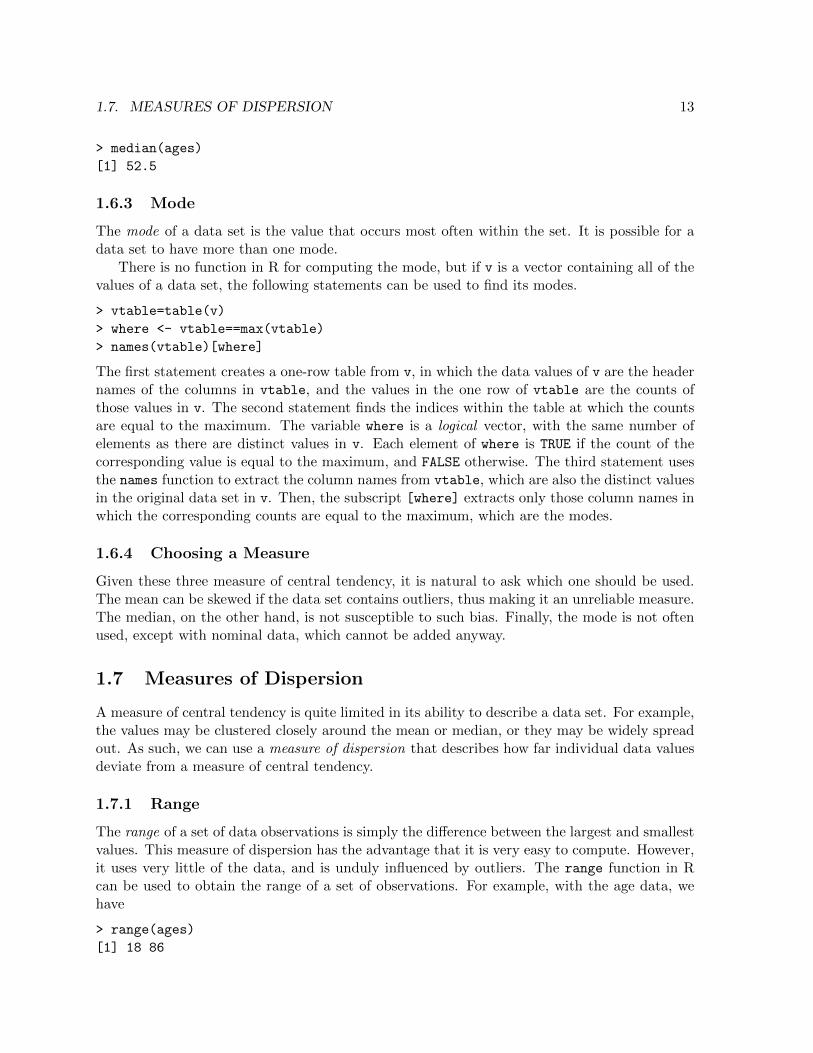
The median of a data set is, informally, the value such that half of the values in the set areless than the median, and half are greater than the median. Specifically, if the number nof observations in the set is odd, then the median is the middle value of the set, at position(n + 1)/2, if the values are sorted. If n is even, then the median is defined to the average ofthe values at positions n/2 and n/2 + 1. The median function in R can be used to compute themedian of a vector of observations. For example, using the age data, we have
1.7. MEASURES OF DISPERSION 13
> median(ages)
[1] 52.5
1.6.3 Mode
The mode of a data set is the value that occurs most often within the set. It is possible for adata set to have more than one mode.
There is no function in R for computing the mode, but if v is a vector containing all of thevalues of a data set, the following statements can be used to find its modes.
> vtable=table(v)
> where <- vtable==max(vtable)
> names(vtable)[where]
The first statement creates a one-row table from v, in which the data values of v are the headernames of the columns in vtable, and the values in the one row of vtable are the counts ofthose values in v. The second statement finds the indices within the table at which the countsare equal to the maximum. The variable where is a logical vector, with the same number ofelements as there are distinct values in v. Each element of where is TRUE if the count of thecorresponding value is equal to the maximum, and FALSE otherwise. The third statement usesthe names function to extract the column names from vtable, which are also the distinct valuesin the original data set in v. Then, the subscript [where] extracts only those column names inwhich the corresponding counts are equal to the maximum, which are the modes.
1.6.4 Choosing a Measure
Given these three measure of central tendency, it is natural to ask which one should be used.The mean can be skewed if the data set contains outliers, thus making it an unreliable measure.The median, on the other hand, is not susceptible to such bias. Finally, the mode is not oftenused, except with nominal data, which cannot be added anyway.
1.7 Measures of Dispersion
A measure of central tendency is quite limited in its ability to describe a data set. For example,the values may be clustered closely around the mean or median, or they may be widely spreadout. As such, we can use a measure of dispersion that describes how far individual data valuesdeviate from a measure of central tendency.
1.7.1 Range
The range of a set of data observations is simply the difference between the largest and smallestvalues. This measure of dispersion has the advantage that it is very easy to compute. However,it uses very little of the data, and is unduly influenced by outliers. The range function in Rcan be used to obtain the range of a set of observations. For example, with the age data, wehave
> range(ages)
[1] 18 86

14 CHAPTER 1. WORKING WITH DATA SETS
1.7.2 Variance
The variance of a population, denoted by σ2, is obtained from the deviation of each observationfrom the mean:
σ2 =1
N
N∑j=1
(xj − µ)2.
An equivalent formula, that is less tedious for larger populations, is
σ2 =
1
N
N∑j=1
x2j
− µ2.
The formula for the variance of a sample, denoted by s2, is slightly different:
s2 =1
n− 1
n∑j=1
(xj − x)2.
The division by (n− 1) instead of n is intended to compensate for the tendency of the samplevariance, when dividing by n, to underestimate the population variance. The var function inR computes the sample variance of a vector of observations that is given as an argument.
1.7.3 Standard Deviation
For both a population and a sample, the standard deviation is the square root of the variance.That is, the standard deviation of a population is
σ =
√√√√ 1
N
N∑j=1
(xj − µ)2,
whereas for a sample, we have
s =
√√√√ 1
n− 1
n∑j=1
(xj − x)2.
An advantage of the standard deviation over the variance, as a measure of dispersion, is thatthe standard deviation is measured using the same units as the original data. The sd functionin R computes the sample standard deviation of a given vector of observations. For example,from the age data, we obtain
> var(ages)
[1] 325.0379
> sd(ages)
[1] 18.02881

1.7. MEASURES OF DISPERSION 15
For grouped data in a relative frequency distribution, with n classes, class values cj (forexample, the midpoint of the values in the class), and relative frequencies fj , j = 1, 2, . . . , n,the population standard deviation can be computed as follows:
σ =
√√√√√ n∑j=1
c2jfj
− µ2.
The empirical rule states that if the distribution of a set of observations is “bell-shaped”,meaning that the distribution is symmetric around the mean and decreases toward zero awayfrom the mean, then approximately 68, 95, and 99.7 % of the observations fall within 1, 2, and 3standard deviations of the mean, respectively. This is illustrated in Figure 1.5. Another rule of
Figure 1.5: Illustration of the empirical rule: for a bell-shaped curve, approximately 68, 95 and99.7% of the observations fall within 1, 2 and 3 standard deviations of the mean, respectively.
thumb, that applies even to distributions that are not bell-shaped or symmetric, is Chebyshev’sTheorem, which states that if k > 1, then at least
(1− 1
k2
)100 % of the observations fall within
k standard deviations of the mean.
1.7.4 Quartiles
Another measure of dispersion is the use of quartiles, which are obtained by dividing a data setinto four segments that, as much as possible, contain an equal number of observations. Justas the median is the “middle” value of the data set, the first quartile, denoted by Q1, is themedian of the “lower half” of the data, and the third quartile, denoted by Q3, is the medianof the “upper half” of the data. There are various ways of determining what constitutes thelower and upper halves; some statisticians include the median in these halves if it is an actualobservation, but some do not.
Once the first and third quartiles are computed, the interquartile range, denoted by IQR,is defined by
IQR = Q3 −Q1.
This value is used to measure the spread of the center half of data, and identify outliers. Arule of thumb is to classify any values less than Q1− 1.5IQR, or greater than Q3 + 1.5IQR, asoutliers.
The following R statements illustrate the computation of Q1, Q3 and the IQR, in order:

16 CHAPTER 1. WORKING WITH DATA SETS
> quantile(ages,0.25)
25%
37.75
> quantile(ages,0.75)
75%
66
> IQR(ages)
[1] 28.25
The five-point summary of a data set consists of the minimum value, Q1, the median (alsodenoted by Q2), Q3, and the maximum value. It can be obtained using the summary functionin R. For example, from the age data, we obtain
> summary(ages)
Min. 1st Qu. Median Mean 3rd Qu. Max.
18.00 37.75 52.50 52.55 66.00 86.00
These measures can be used to construct a box-and-whisker plot , which displays the interquartilerange and outliers. A box is drawn with opposing boundaries placed at Q1 and Q3, with aparallel line drawn within the box at the median. Then, perpendicular lines, which are the“whiskers”, are drawn from Q1 to the minimum value, and from Q3 to the maximum value.The length of the box is equal to IQR, and if the length of either of the whiskers is more than1.5 times the width of the box, then the value at the end of the whisker is an outlier.
A box-and-whisker plot can be produced in R using the boxplot command. For example,the plot shown in Figure 1.6 is obtained from the age data used in earlier examples using thecommand
boxplot(ages)
1.8 Exercises
1. In a survey of 100 stocks on NASDAQ, the average percent increase for the past year was9% for NASDAQ stocks.
(a) The “average increase” for all NASDAQ stocks is the:
A. parameter
B. population
C. sample
D. statistic
(b) All of the NASDAQ stocks are the:
A. parameter
B. population
C. sample
D. statistic
(c) Nine percent is the:

1.8. EXERCISES 17
Figure 1.6: Box-and-whisker plot produced from age data
A. parameter
B. population
C. sample
D. statistic
(d) The 100 NASDAQ stocks in the survey are the:
A. parameter
B. population
C. sample
D. statistic
(e) The data collected would be
A. qualitative
B. quantitative discrete
C. quantitative continuous
D. qualitative discrete
2. Thirty people spent two weeks celebrating Mardi Gras in New Orleans. Their two-weekweight gain is below. (Note: a loss is shown by a negative weight gain.)

18 CHAPTER 1. WORKING WITH DATA SETS
Weight Gain Frequency
-2 3-1 50 21 44 136 2
11 1
Calculate the standard deviation.
3. A sociologist wants to know what employed adult women think about government fund-ing for day care. The sociologist obtains a list of 520 members of a local business andprofessional women’s club and mails a questionnaire to 100 of these women selected atrandom. Sixty-eight questionnaires are returned. What is the population in this study?
A. all employed adult women
B. all employed women with children
C. the 100 women who received the questionnaire
D. all the members of a local business and professional women’s club
4. A sample of pounds lost, in a certain month, by individual members of a weight reducingclinic produced the following statistics: Mean = 5 lbs. Median = 4.5 lbs. Mode = 4 lbs.Standard deviation = 3.8 lbs. First quartile = 2 lbs. Third quartile = 8.5 lbs.
Which of the following is a correct statement based on the information above?
A. One fourth of the members lost exactly two pounds.
B. The middle fifty percent of the members lost from two to 8.5 lbs.
C. Most people lost 3.5 to 4.5 lbs.
D. One fourth of the members lost exactly 8.5 pounds.
5. What does it mean when a data set has a standard deviation equal to zero?
A. There are no data to begin with.
B. The mean of the data is also zero.
C. All of the data have the same value.
D. All values of the data appear with the same frequency.
6. Rachel’s piano cost $3,000. The average cost for a piano is $4,000 with a standarddeviation of $2,500. Becca’s guitar cost $550. The average cost for a guitar is $500with a standard deviation of $200. Matt’s drums cost $600. The average cost for drumsis $700 with a standard deviation of $100. Whose cost was lowest when compared to hisor her own instrument?
7. Which of the following is true for the box plot in Figure 1.7?

1.8. EXERCISES 19
Figure 1.7: Box plot for Exercise 7
A. There are no data values of three.
B. Fifty percent of the data are four.
C. Twenty-five percent of the data are at most five.
D. There is about the same amount of data from 4-5 as there is from 5-7.
8. The interest rate charged on financial aid is what kind of data?
A. qualitative
B. qualitative discrete
C. quantitative discrete
D. quantitative continuous
9. The following information is about the students who receive financial aid at the localcommunity college. 1st quartile = $250, 2nd quartile = $700, 3rd quartile = $1200
These amounts are for the school year. If a sample of 200 students is taken, how manyare expected to receive $250 or more?
A. 50
B. 150
C. 250
D. cannot be determined
10. Ninety homeowners were asked the number of estimates they obtained before having theirhomes fumigated. Let X = the number of estimates.
x Relative Frequency Cumulative Relative Frequency
1 0.32 0.24 0.45 0.1
(a) Complete the cumulative frequency column.
(b) Calculate the sample mean.
(c) Calculate the median, M , the first quartile, Q1, and the third quartile, Q3.

20 CHAPTER 1. WORKING WITH DATA SETS
11. The mean grade on a math exam in Rachel’s class was 74, with a standard deviation offive. Rachel earned an 80. The mean grade on a math exam in Becca’s class was 47, witha standard deviation of two. Becca earned a 51. The mean grade on a math exam inMatt’s class was 70, with a standard deviation of eight. Matt earned an 83.
Find whose score was the best, compared to his or her own class. Justify your answernumerically.
A. Matt
B. Becca
C. Rachel
D. All scores were equally good.
12. Identify each of the following statistics as either descriptive or inferential.
(a) Seventy-six percent of households in the United States own a computer.
(b) Households with income more than $150,000 are more likely to have access to theinternet (86 percent) than households with income under $25,000 (50 percent).
(c) Wilt Chamberlain scored 31,419 points in his NBA career.
(d) The average SAT score among Stanford students is 1475.
(e) In a recent poll, 44% of Americans had a favorable opinion of the President of theUnited States.
13. Classify the following data as nominal, ordinal, interval or ratio.
(a) Average monthly temperature in degrees Fahrenheit for the city of Palo Alto through-out the year
(b) Average monthly rainfall in inches for the city of Seattle throughout the year
(c) Education level of survey respondents:
Level Number of RespondentsLess than high school 24,960High school or GED 61,952Some college or associate’s degree 53,255Bachelor’s degree or higher 6,130
(d) Employment status of survey respondents:
Level Number of RespondentsEmployed 140,696Unemployed 14,711Not in labor force 88,282
(e) Age of respondents in the survey
(f) Gender of the respondents in the survey
(g) The year in which a respondent was born

1.8. EXERCISES 21
(h) The state in which a respondent resides
(i) The race of the respondents in the survey classified as White, African-American,Asian or Hispanic
(j) Student evaluation rating of an instructor as Excellent, Good, Fair, or Poor
(k) The uniform number of each member of a football team
(l) A list of graduating high school seniors, sorted by class rank
(m) Final exam scores in a class, on a scale of 0 to 100
14. Construct a frequency distribution of the following set of ages of respondents, with 6classes ranging from 20 to 49.
44 28 48 43 40 4046 36 34 48 42 2124 48 43 39 42 2846 48 24 21 31 2138 25 32 45 39 2323 48 47 47 25 44
15. Construct a histogram using the solution from Problem 14.
16. Construct a relative and a cumulative frequency distribution from the data in Problem14.
17. Construct a pie chart from the solution to Problem 14.
18. Construct a stem-and-leaf diagram from the data in Problem 14 using stems for the scoresin the 20s, 30s, and 40s.
19. Calculate the mean, median, mode, variance, standard deviation, and range for the fol-lowing data set:
20,15,24,10,8,19,24,12,21,6,8,11,6,2,11,6,5,6,10.
20. The following table is a frequency distribution of exam scores. Compute the mean score,and the standard deviation for the score, from the given frequency distribution.
Score Range Number of Students40-49 750-59 3660-69 2670-79 4580-89 2490-99 12
21. Given the following homework averages, quiz averages, and exam scores, compute theoverall averages using the following weights: quizzes count 10%, homework counts 20%,midterm exam counts 30%, and final exam counts 40%.

22 CHAPTER 1. WORKING WITH DATA SETS
Quiz Homework Midterm Final80 90 77 8395 95 91 6273 79 75 71
22. A data set that follows a bell-shaped and symmetrical distribution has a mean equal to50 and a standard deviation equal to 5. What range of values centered around the meanwould represent 68 percent of the data points?
23. A data set that is not bell-shaped or symmetrical has a mean equal to 75 and a standarddeviation equal to 8. What is the minimum percent of values that would fall between 59and 91?

Chapter 2
Probability
2.1 Introduction
2.1.1 Events
Informally, probability is the likelihood that a particular event will occur. To be able to computeprobabilities, though, we need precise definitions of the concepts included in this informaldefinition.
• An experiment is a process of measuring or observing an activity for the purpose ofcollecting data.
• An outcome is a result of an experiment.
• A sample space is a set of all possible outcomes of an experiment.
• An event is an outcome, or a set of outcomes, of interest. Mathematically, an event is asubset of the sample space.
2.1.2 Types of Probability
Now, we can formulate a precise definition of probability. Classical probability is the numberof outcomes contained in an event, relative to size of sample space. That is, if E is an event,and S is the sample space, then the probability of E, denoted by P (E), is defined by
P (E) =|E||S|
,
where, for any set A, |A| denotes the cardinality of A, which is simply the number of elementscontained in A.
Example Consider the result of rolling a single six-sided die, which is an experiment. Theoutcome is the number showing on the die after it is rolled. The sample space is the setS = {1, 2, 3, 4, 5, 6}, which contains all possible results of the die roll. Examples of events would
23

24 CHAPTER 2. PROBABILITY
be “rolling a 6”, which is the set {6}, or “rolling an odd number”, which is the set {1, 3, 5}. IfE is the event “rolling a number higher than 4”, which is the set {5, 6}, then
P (E) =|E||S|
=2
6=
1
3.
2
There are other types of probability. Empirical probability is defined to be the frequency ofan event relative to the number of observations. The distinction between classical probabilityand empirical probability is based on the distinction between an entire population and a sampleof that population. Classical probability describes the likelihood of an event, relative to anexhaustive set of all possible outcomes that is its sample space, whereas empirical probabilityhas, as its sample space, the outcomes of a relatively small number of experiments.
An example of empirical probability would be the likelihood that a particular train willbe late. It is not practical to measure this likelihood using classical probabiltiy, which wouldinvolve enumerating a very large set of combinations of circumstances that determine whetherthe train is late or not. To use empirical probability, one could record whether the train waslate or not over a period of time, say several weeks. Then, the sample space consists of thosedays on which the arrival time of the train was recorded, and the event consists of those dayson which the train arrived late. If enough observations are made, then the empirical probabilityis likely very close to what the classical probability would be, if it could be measured.
Finally, subjective probability is probability that is based on intuition rather than experi-ments. For example, my intuition tells me that for any student taking this course, the probabil-ity that they will actually do the exercises is approximately 1/2. I do not have any experimentsto support this statement; rather, it is based on observations of similar behavior over thecourse of my career, and what I know about students at Stanford as opposed to students atother universities.
2.1.3 Properties of Probability
Regardless of the type of probability that is being measured, there are certain properties thatthe probability of an event E must satisfy.
1. P (E) = 1 if the event E is certain to occur.
2. P (E) = 0 if it is certain that E will not occur.
3. P (E) must satisfy 0 ≤ P (E) ≤ 1.
4. If E1, E2, . . . , En are mutually exclusive events, meaning that no two of these events canoccur simultaneously, then
P (E1 ∪ E2 ∪ · · · ∪ En) = P (E1) + P (E2) + · · ·+ P (En) =n∑i=1
P (Ei).
5. A consequence of the first and fourth properties is that if we denote by E′ the complementof an event E, which consists of all outcomes in the sample space that are not containedin E, then
P (E′) = 1− P (E),

2.2. CONDITIONAL PROBABILITY 25
because either E or E′ is certain to occur, due to all outcomes in the sample spacebelonging to one event or the other, but not both.
Example As examples of these properties, let E be the event that the sun is going to risetomorrow. As the often-used quintessential certainty, it is safe to say that P (E) = 1. Afterlimited experimentation, I believe it is equally safe to say that if L is the event in which I willever choose winning lottery numbers, then P (L) = 0, and this will certainly be the case if Imake the wise choice to give up on playing. There is no circumstance under which an eventcan have a negative probability, or a probability greater than 1.
If A is the event that a student earns an A in a particular course, and B is the event thatthey earn a B, and so on, then these events are mutually exclusive, since the student can onlybe assigned one grade. Therefore,
P (A ∪B ∪ C ∪D ∪ F ) = P (A) + P (B) + P (C) + P (D) + P (F ).
2
2.2 Conditional Probability
Simple probability , also known as prior probability , is probability that is determined solely fromthe number of observations of an experiment. On the other hand, conditional probability , alsoknown as posterior probability , is the probability that an event A will occur, given that anotherevent B has already occurred. It is denoted by P (A|B); some sources use the notation P (A/B).
One can think of conditional probability as using a reduced sample space. When measuringP (A|B), one is not considering the whole of the sample space from which A and B originate;instead, one is only considering the subset B of that sample space, and then determining howmany elements of that subset also belong to A.
2.3 Independent Events
Informally, two events A and B are said to be independent if neither one is influenced by theother. Mathematically, we say that A is independent of B if
P (A|B) = P (A).
Example Let A be the event that John is late for work, and B be the event that Jane, whohas no connection to John whatsoever and in fact lives and works in a different city from John,is late for work. These two events are independent, so P (A|B) = P (A). On the other hand,suppose John drives to work and that C is the event that there is a major traffic jam in his city.This event, if it occurs, could cause him to be late for work, so P (A) is influenced by P (C).That is, P (A) is not the same as P (A|C). On the other hand, B and C are independent, soP (B|C) = P (B). 2
26 CHAPTER 2. PROBABILITY
2.4 Intersection of Events
Let A and B be two events. Then, the joint probability of A and B, denoted by A ∩ B, isthe event consisting of all outcomes that belong to both A and B. Since events are defined tobe subsets of the sample space, the joint probability of events is simply the intersection of thecorresponding sets.
Joint probabilities arise in contingency tables, which list the number of outcomes that cor-respond to each possible pairing of results of two experiments. In a contingency table, each rowcorresponds to a value of one variable (that is, one possible result of an experiment), and eachcolumn corresponds to a value of a second variable. Then, the entry in row i, column j of thetable is the number of outcomes corresponding to the ith value of the first variable and the jthvalue of the second.
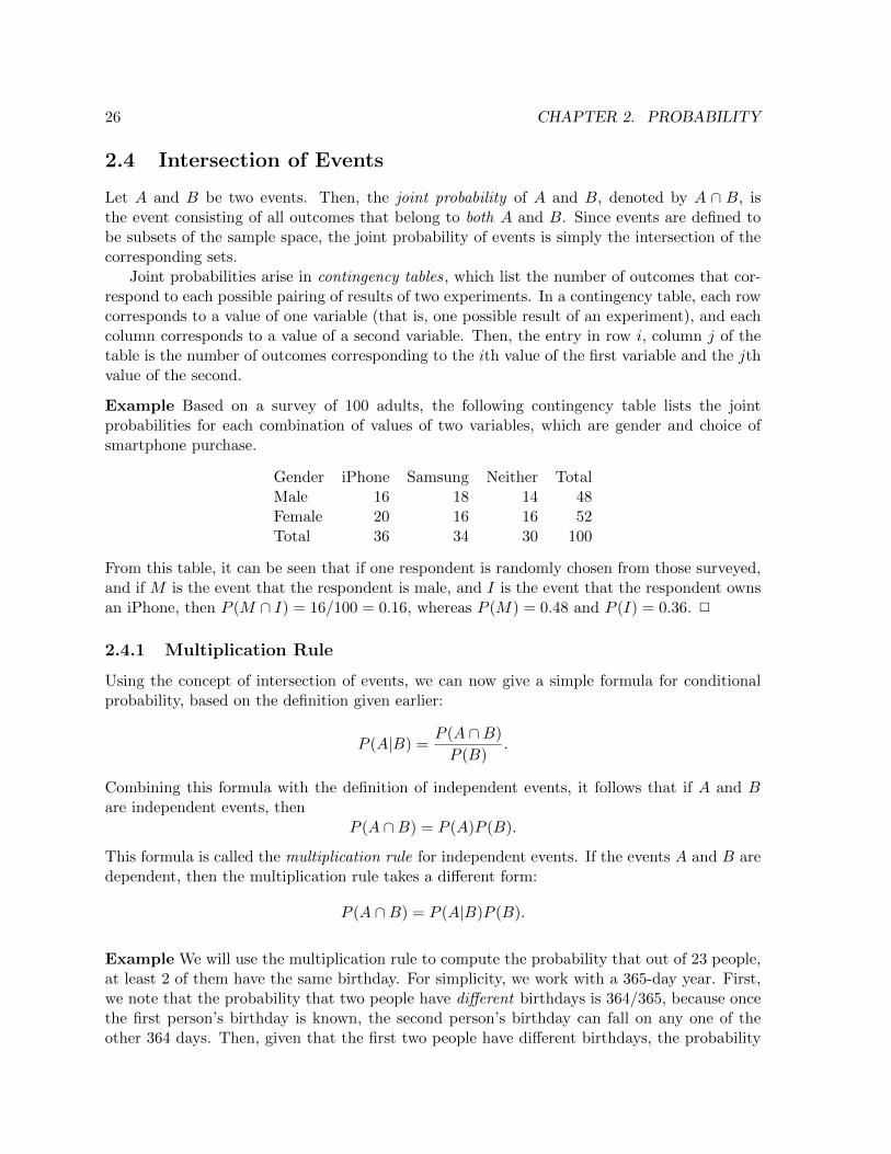
Example Based on a survey of 100 adults, the following contingency table lists the jointprobabilities for each combination of values of two variables, which are gender and choice ofsmartphone purchase.
Gender iPhone Samsung Neither TotalMale 16 18 14 48Female 20 16 16 52Total 36 34 30 100
From this table, it can be seen that if one respondent is randomly chosen from those surveyed,and if M is the event that the respondent is male, and I is the event that the respondent ownsan iPhone, then P (M ∩ I) = 16/100 = 0.16, whereas P (M) = 0.48 and P (I) = 0.36. 2
2.4.1 Multiplication Rule
Using the concept of intersection of events, we can now give a simple formula for conditionalprobability, based on the definition given earlier:
P (A|B) =P (A ∩B)
P (B).
Combining this formula with the definition of independent events, it follows that if A and Bare independent events, then
P (A ∩B) = P (A)P (B).
This formula is called the multiplication rule for independent events. If the events A and B aredependent, then the multiplication rule takes a different form:
P (A ∩B) = P (A|B)P (B).
Example We will use the multiplication rule to compute the probability that out of 23 people,at least 2 of them have the same birthday. For simplicity, we work with a 365-day year. First,we note that the probability that two people have different birthdays is 364/365, because oncethe first person’s birthday is known, the second person’s birthday can fall on any one of theother 364 days. Then, given that the first two people have different birthdays, the probability

2.4. INTERSECTION OF EVENTS 27
that the third person has a different birthday is 363/365. Continuing this process, if we letAi be the event that the ith person has a different birthday than the first i − 1 people, theprobability that all 22 people have different birthdays is
P (A23 ∩A22 ∩ · · · ∩A2) = P (A2)P (A3|A2)P (A4|A2 ∩A3) · · ·P (A23|A2 ∩A3 ∩ · · · ∩A22)
=364
365
363
365· · · 343
365= 0.493.
Therefore, the probability that at least two of the 23 people have the same birthday is 1−0.493 =0.507. That is, there is a 50% chance that at least two of them have the same birthday. 2
Example To illustrate the formula for conditional probability and the multiplication rule, werevisit the previous example with the contingency table. As before, let M be the event that arandomly chosen respondent is male, and let I be the event that they own an iPhone. Then
P (M |I) =P (M ∩ I)
P (I)=
0.16
0.36= 0.4.
This can also be seen by considering only the column of the table that corresponds to iPhoneowners: there are 36 respondents who are iPhone owners, and 16 of those are male, so basedon that, P (M |I) = 16/36 = 0.4.
The table can be used to determine whether the events M and I are independent. We knowthat P (M ∩ I) = 0.16. From the totals of the first row and first column of the table, we haveP (M) = 0.48 and P (I) = 0.36. However, because
P (M)P (I) = (0.48)(0.36) = 0.1728 6= P (M ∩ I),
we conclude that these events are dependent .On the other hand, suppose two six-sided die are rolled. The number shown on each die is
independent of the other, and since the probability of either die roll being a 6 is 1/6, we canconclude that the probability of rolling double sixes is (1/6)(1/6) = 1/36. 2
To reinforce the notion that conditional probability is the probability of an event withrespect to a reduced sample space, we note that if S is the original sample space, then
P (A|B) =P (A ∩B)
P (B)
=|A ∩B|/|S||B|/|S|
=|A ∩B||B|
.
That is, P (A|B) is obtained by restricting the sample space to all outcomes in B.
2.4.2 Mutually Exclusive Events
Two events A and B are said to be mutually exclusive if it is not possible for A and B to occursimultaneously. In set notation, we say that A and B are disjoint , or that A∩B =. Since thereare no outcomes that belong to both A and B, it follows that for mutually exclusive events Aand B,
P (A ∩B) = 0.

28 CHAPTER 2. PROBABILITY
2.5 Union of Events
The union of two events A and B is the event consisting of all outcomes that belong to eitherA or B (and possibly both; the “or” is inclusive). Using set notation again, we denote thisevent by A ∪B.
2.5.1 Addition Rule
If two events A and B are mutually exclusive, then, from one of the properties of probabilitystated earlier, it follows that
P (A ∪B) = P (A) + P (B).
On the other hand, if A and B are not mutually exclusive, then the above formula does nothold, because outcomes that are in both A and B end up being counted twice. Therefore, weneed to correct the formula as follows:
P (A ∪B) = P (A) + P (B)− P (A ∩B).
Example Consider the act of drawing a single card from a standard 52-card deck. Let A bethe event that the card drawn is a spade, let B be the event that the card drawn is a heart, andlet C be the event that the card drawn is a face card (jack, queen or king). Then, the events Aand B are mutually exclusive, but the events A and C are not, because it is possible to draw ajack, queen or king of spades. From
P (A) = P (B) =1
4, P (C) =
3
13, P (A ∩ C) =
3
52,
we obtain
P (A ∪B) = P (A) + P (B) =1
4+
1
4=
1
2,
and
P (A ∪ C) = P (A) + P (C)− P (A ∩ C) =1
4+
3
13− 3
52=
11
26.
2
2.6 Bayes’ Theorem
Given two events A and B, Bayes’ Theorem is a result that relates the conditional probabilitiesP (A|B) and P (B|A). It states that
P (B|A) =P (B)P (A|B)
P (B)P (A|B) + P (B′)P (A|B′). (2.1)
To see why this theorem is true, note that by the multiplication rule, the numerator on theright-hand side is simply P (A ∩ B), and the denominator becomes P (A ∩ B) + P (A ∩ B′).Because B and B′ are mutually exclusive, but also exhaustive (meaning B ∪B′ is equal to theentire sample space), this expression becomes P ((A ∩ B) ∪ (A ∩ B′)) = P (A). We thereforehave
P (B|A) =P (A ∩B)
P (A),

2.7. COUNTING PRINCIPLES 29
which can be rearranged to again obtain the multiplication rule. Also, if we keep the originalnumerator in (2.1) but use the simplified denominator, we obtain another commonly usedstatement of Bayes’ Theorem,
P (B|A) =P (B)P (A|B)
P (A). (2.2)
This form is very useful for computing one conditional probability from another that may beeasier to obtain.
Example Suppose an insurance company classifies people as accident-prone or not accident-prone. Furthermore, they determine that the probability of an accident-prone person actuallyhaving an accident within the next year is 0.4, whereas the probability of a non-accident-proneperson having an accident within the next year is 0.2. If 30% of people are accident-prone, thenwhat is the probability that someone who does have an accident within the next year actuallyis accident-prone?
To answer this question, we let A be the event that the person has an accident within thenext year, and let B be the event that the person is accident-prone. From the given information,we have
P (A|B) = 0.4, P (A|B′) = 0.2, P (B) = 0.3.
From these probabilities, we conclude that
P (A) = P (A|B)P (B) + P (A|B′)P (B′) = (0.4)(0.3) + (0.2)(0.7) = 0.26.
Using Bayes’ Theorem, we conclude that the probability of someone who has an accident beingaccident-prone is
P (B|A) =P (B)P (A|B)
P (A)=
(0.3)(0.4)
0.26= 0.4615.
2
2.7 Counting Principles
In order to compute probabilities using the definition, it is necessary to be able to determine thenumber of outcomes in an event or a sample space. In this section, we present some techniquesfor counting how many elements are in a given set.
2.7.1 The Fundamental Counting Principle
The Fundamental Counting Principle states that if there are m ways to perform task A, and nways to perform task B, then
• The number of ways to perform task A and task B is mn, and
• The number of ways to perform task A or task B (but not both) is m+ n.
Example Suppose that an ice cream shop offers a selection of ten different flavors, five differenttoppings, and three different sizes. Then the number of possible orders of ice cream is 10(5)(3) =150. On the other hand, suppose that at a particular restaurant, one entree selection offers

30 CHAPTER 2. PROBABILITY
either steak or chicken, and a choice of a side dish. If there are 7 different steak selections, 4different chicken selections, and 10 side dishes, then the number of possible variations of thisentree are (7 + 4)10 = 110. 2
Example Standard license plates in California have a digit, followed by 3 letters, followed byanother 3 digits. Therefore, the number of possible license plates is
10 · 26 · 26 · 26 · 10 · 10 · 10 = 104263 = 175, 760, 000.
2
It can be seen from this example that if there are n ways to perform a certain task, and it mustbe performed r times, then the number of ways to do so is nr.
2.7.2 Permutations
In many situations, it is necessary to know the number of possible arrangements of things, orthe number of ways to perform a task in which there is some sort of ordering. Equivalently, itis often necessary to sample a number of objects in such a way that (1) the order in which theobjects are sampled is relevant, and (2) after an object is sampled, it is removed from the setso that it cannot be chosen again (this is known as sampling without replacement). To see theequivalence, consider the task of arranging n objects. Once an object is assigned its position,it should not be considered when placing the second object, and then the second object shouldnot be considered when placing the third, and so on.
To sample r objects, in order, from a set of n, without replacement, we first note that thereare n ways to choose the first object. Then, the chosen object is removed from consideration,meaning that there n − 1 ways to choose the second object. Then, that object is removedconsideration, leaving n− 2 ways to choose the third object, and so on. Therefore, the numberof ways to choose r objects from a set of n, without replacement, is
n(n− 1)(n− 2) · · · (n− r + 1) =n!
(n− r)!= nPr.
Since this is also the number of ways to arrange r objects chosen from a set of n, we call thisthe number of permutations of these objects.
Example Suppose that a club has 25 members, and it is necessary to elect a president, vice-president, secretary, and treasurer. Then, the number of ways to choose 4 members to fill thesepositions is
25P4 =25!
(25− 4)!= 25 · 24 · 23 · 22 = 303, 600.
2
Example We know from the Fundamental Counting Principle that the number of possible4-letter words is 264. This is in instance of sampling with replacement, because once the firstletter is chosen, it can be chosen again for the second letter, and so on. However, if we requirethat all of the letters in each word are different, then we must sample without replacement, sothe number of such words is 26P4 = 26(25)(24)(23). 2

2.8. EXERCISES 31
2.7.3 Combinations
It is often the case that a number of objects must be sampled without replacement, but theorder in which they are sampled is irrelevant. In order to determine the number of ways inwhich such a sampling may be performed, we can start by computing nPr, where n is thenumber of objects to choose from and r is the number of objects to be chosen, but then wemust divide by rPr = r!, the number of ways to arrange r objects. The result is
nCr =
(nr
)=
n!
r!(n− r)!,
which is called the number of combinations of r objects chosen from a set of n, also referredto as “n-choose-r”. It is also the known as a binomial coefficient , as it arises naturally whencomputing powers of binomials.
Example Suppose we wish to count the number of possible poker hands. This means countingthe number of ways to choose 5 cards from a deck of 52. The number in which the cards arechosen is irrelevant, so we use combinations instead of permutations. The number of hands is
52C5 =52!
5!(52− 5)!=
52 · 51 · 50 · 49 · 48
5 · 4 · 3 · 2 · 1= 2, 598, 960.
2
Example As another example, consider the 25-member club from the discussion of permuta-tions. Suppose that they need to form a 4-person committee. The number of ways to do thisis 25C4, the number of ways to choose 4 members from a set of 25. The reason why 25C4 isused here, as opposed to 25P4 for electing 4 officers, is that a member’s position within thecommittee is irrelevant, whereas once 4 members are chosen to be officers, it matters which oneof them is chosen to be president, which is chosen to be vice-president, and so on. 2
2.7.4 Permutations and Combinations in R
In R, the choose and factorial functions can be used to compute the quantities nPr and
nCr. To compute nCr, use choose(n,r). To compute nPr, use choose(n,r)*factorial(r).The combn function can be used to actually enumerate all of the combinations of elements of avector. For example, the combinations of 3 numbers chosen from the set {1, 2, 3, 4, 5} are
> v=c(1:5)
> combn(v,3)
[,1] [,2] [,3] [,4] [,5] [,6] [,7] [,8] [,9] [,10]
[1,] 1 1 1 1 1 1 2 2 2 3
[2,] 2 2 2 3 3 4 3 3 4 4
[3,] 3 4 5 4 5 5 4 5 5 5
2.8 Exercises
1. A recent poll concerning credit cards found that 35 percent of respondents use a creditcard that gives them a mile of air travel for every dollar they charge. Thirty percent of

32 CHAPTER 2. PROBABILITY
the respondents charge more than $2,000 per month. Of those respondents who chargemore than $2,000, 80 percent use a credit card that gives them a mile of air travel forevery dollar they charge.
(a) What is the probability that a randomly selected respondent will spend more than$2,000 AND use a credit card that gives them a mile of air travel for every dollarthey charge?
(b) Are using a credit card that gives a mile of air travel for each dollar spent ANDcharging more than $2,000 per month independent events?
A. Yes
B. No, but they are mutually exclusive.
C. No, and they are not mutually exclusive either.
D. Not enough information given to determine the answer
2. If P (G|H) = P (G) and P (G) > 0, then which of the following is correct?
A. P (G) = P (H)
B. G and H are independent events.
C. G and H are mutually exclusive events.
D. Knowing that H has occurred will affect the chance that G will happen.
3. Assume the following: P (A) = 0.2, P (B) = 0.3; A and B are independent events.
(a) P (A ∩B) =
(b) P (A ∪B) =
4. In a survey at Kirkwood Ski Resort the following information was recorded:
Age 0-10 11-20 21-40 40+
Ski 10 12 30 8Snowboard 6 17 12 5
Suppose that one person from the above table was randomly selected.
(a) Find the probability that the person was a skier or was age 11-20.
(b) Find the probability that the person was a snowboarder given he or she was age21-40.
5. Which of the following statements are true?
A. Sport and age are independent events.
B. Ski and age 11-20 are mutually exclusive events.
C. P (Ski ∩ age21− 40) < P (Ski|age21− 40)
D. P (Snowboard ∪ age0− 10) < P (Snowboard|age0− 10)

2.8. EXERCISES 33
6. A game is played with the following rules: it costs $10 to enter. A fair coin is tossed fourtimes. If you do not get four heads or four tails, you lose your $10. If you get four headsor four tails, you get back your $10, plus $30 more. Over the long run of playing thisgame, what are your expected earnings?
7. Suppose that the probability of a drought in any independent year is 20%. Out of thoseyears in which a drought occurs, the probability of water rationing is 10%. However, inany year, the probability of water rationing is 5%.
(a) What is the probability of both a drought and water rationing occurring?
(b) Out of the years with water rationing, find the probability that there is a drought.
8. Define each of the following as classical, empirical, or subjective probability.
(a) The probability that Tom Brady will throw a touchdown pass on the next play.
(b) The probability of drawing a face card from a deck of cards.
(c) The probability of winning my next game of Words with Friends.
(d) The probability of winning the next drawing in the California lottery.
(e) The probability that I will get a flat tire sometime this summer.
(f) The probability that I will finish writing these notes before the course begins.
9. Identify whether each of the following are valid probabilities.
(a) 75 percent
(b) 1.9
(c) 110 percent
(d) −3.1
(e) 0.65
(f) 0
10. A survey of 293,415 individuals asked whether they lived in a home that had at least onecomputer. Each individual was classified by household income. The contingency table isshown here.
Household Income Computer No Computer TotalLess than $25,000 39,901 30,451 70,352$25,000-$49,999 58,396 18,589 76,985$50,000-$99,999 82,408 7,106 89,514$100,000-$149,999 31,862 1,295 33,157$150,000 or more 22,499 908 23,407Total 235,066 58,349 293,415
An individual from the survey is randomly selected. We define:
Event A: The selected individual has a computer in their home.

34 CHAPTER 2. PROBABILITY
Event B: The selected individual has a household income between $50,000 and $99,999.
For each of the following, express the given probability in terms of events, e.g. P (A) orP (B|A), in addition to computing its numerical value.
(a) Determine the probability that the selected individual has a computer in their home.
(b) Determine the probability that the selected individual has a household income be-tween $50,000 and $99,999.
(c) Determine the probability that the selected individual has a computer in their home,and has a household income between $50,000 and $99,999.
(d) Determine the probability that the selected individual has a computer in their home,or has a household income between $50,000 and $99,999.
11. A poll of 300 voters asked whether they were in favor or not in favor of a particularlaw. Each person was identified as Republican, Democrat, or independent. The followingcontingency table shows the results.
Party In Favor Not in Favor TotalRepublican 94 64 158Democrat 48 65 113Independent 25 14 39
A respondent from the poll is randomly selected. We define:
Event A: The respondent is in favor of the law.
Event B: The respondent is a Democrat.
Event C: The respondent is a Republican.
For each of the following, express the given probability in terms of events, e.g. P (A) orP (B|A), in addition to computing its numerical value.
(a) Determine the probability that the respondent is in favor of the law.
(b) Determine the probability that the respondent is a Democrat.
(c) Determine the probability that the respondent is not in favor of the law.
(d) Determine the probability that the respondent is a Republican or independent.
(e) Determine the probability that the respondent is in favor of the law, given that theperson is a Democrat.
(f) Determine the probability that the respondent is not in favor of the law, given thatthe person is a Democrat.
(g) Determine the probability that the respondent is in favor of the law, given that theperson is a Republican.
(h) Determine the probability that the respondent is in favor of the law and that theperson is a Democrat.
(i) Determine the probability that the respondent is in favor of the law and that theperson is a Republican.

2.8. EXERCISES 35
(j) Determine the probability that the respondent is in favor of the law or that theperson is a Democrat.
(k) Determine the probability that the respondent is in favor of the law or that theperson is a Republican.
(l) Using Bayes’ Theorem, compute the probability that the respondent is a Republican,given that the person is in favor of the law.
12. A restaurant has a menu with five appetizers, seven entrees, and three desserts. Howmany different meals can be ordered?
13. A multiple-choice test has 20 questions, with each question having five choices. What isthe probability that a student answers every question correctly using random guessing?
14. In a race with 10 runners, how many ways can the runners finish first, second and third?
15. A panel of 12 jurors needs to be selected from a group of 60 people. How many differentjuries can be selected?
16. What is the probability of being dealt a straight flush (five cards in sequence, all of thesame suit) in five-card poker?

36 CHAPTER 2. PROBABILITY

Chapter 3
Probability Distributions
3.1 Introduction
Now that we know how to compute probabilities of events, we can study the behavior ofthe probability across all possible outcomes of an experiment–that is, the distribution of theprobability across the sample space. Our understanding of the probability distribution willeventually allow us to make inferences from the data from which the distribution arises.
3.1.1 Random Variables
A random variable, usually denoted by a capital letter such asX, is an outcome of an experimentthat has a numerical value. The value itself is usually denoted by the lower-case version of theletter used to denote the variable itself; that is, a random variable X takes on numerical valuesthat are denoted by x. Random variables can either be continuous or discrete. A continuousrandom variable can assume a value equal to any real number within some interval, whereasa discrete random variable can only assume selected numerical values, such as, for example,nonnegative integers. We will study random variables of both kinds.
3.1.2 Discrete Probability Distributions
A discrete probability distribution is a listing of all possible values of a discrete random variable,along with the probability of each value being assumed by the variable.
Example Let X be a discrete random variable whose outcomes correspond to where one finishesin a race: first, second, third, etc. If there are 10 runners in the race, then X can assume as avalue any positive integer between 1 and 10. The probability distribution might look like thefollowing:
37
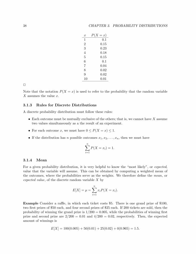
38 CHAPTER 3. PROBABILITY DISTRIBUTIONS
x P (X = x)
1 0.12 0.153 0.234 0.185 0.156 0.17 0.048 0.029 0.0210 0.01
2
Note that the notation P (X = x) is used to refer to the probability that the random variableX assumes the value x.
3.1.3 Rules for Discrete Distributions
A discrete probability distribution must follow these rules:
• Each outcome must be mutually exclusive of the others; that is, we cannot have X assumetwo values simultaneously as a the result of an experiment.
• For each outcome x, we must have 0 ≤ P (X = x) ≤ 1.
• If the distribution has n possible outcomes x1, x2, . . . , xn, then we must have
n∑i=1
P (X = xi) = 1.
3.1.4 Mean
For a given probability distribution, it is very helpful to know the “most likely”, or expected,value that the variable will assume. This can be obtained by computing a weighted mean ofthe outcomes, where the probabilities serve as the weights. We therefore define the mean, orexpected value, of the discrete random variable X by
E[X] = µ =n∑i=1
xiP (X = xi).
Example Consider a raffle, in which each ticket costs $5. There is one grand prize of $100,two first prizes of $50 each, and four second prizes of $25 each. If 200 tickets are sold, then theprobability of winning the grand prize is 1/200 = 0.005, while the probabilities of winning firstprize and second prize are 2/200 = 0.01 and 4/200 = 0.02, respectively. Then, the expectedamount of winnings is
E[X] = 100(0.005) + 50(0.01) + 25(0.02) + 0(0.965) = 1.5.
3.2. UNIFORM DISTRIBUTION 39
That is, a ticket holder can expect to win, on average, $1.50. However, we must account forthe cost of the ticket, which applies to all participants; therefore, the expected net winnings is−$3.50. Since the expected amount is negative, the raffle is not fair to the ticket holders; if theexpected value was zero, then the raffle would be considered a “fair game”. 2
3.1.5 Variance and Standard Deviation
Using the mean of X, we can then characterize the dispersion of the outcomes by defining thevariance of X as follows:
σ2 =n∑i=1
(xi − µ)2P (X = xi).
An equivalent formula, in terms of expected values, is
σ2 = E[X2]− E[X]2.
Note that in the first term, the values of X are squared, and then they are multiplied by theprobabilities and summed, whereas in the second term, the expected value is computed first,and then squared.
3.2 Uniform Distribution
The uniform distribution U{a, b} is the probability distribution for a random variable X withdomain {a, a+1, . . . , b} in which each value in the domain of X is equally likely to be observed.It follows that the probability mass function for this distribution is
P (X = k) =1
n, n = b− a+ 1, k ∈ {a, a+ 1, . . . , b}.
Using the above definitions of the mean and variance of a discrete random variable, it can beshown that
E[X] =a+ b
2, σ2 =
(b− a+ 1)2 − 1
12.
If a random variable X has the distribution U{a, b}, we write X ∼ U{a, b}. We will use similarnotation with other probability distributions, in order to indicate that a given random variablehas a particular distribution.
3.3 Binomial Distribution
3.3.1 Binomial Experiments
Suppose that an experiment is performed n times, and it can have only two outcomes, thatare classified as “success” and “failure”. Each of these individual experiments is referred toas a trial . Furthermore, suppose that each trial is independent of the others, and that theprobability of a trial being successful is p, where 0 < p < 1 (and therefore, the probability offailure is q = 1− p). These trials are called Bernoulli trials.
Examples of Bernoulli trials are:

40 CHAPTER 3. PROBABILITY DISTRIBUTIONS
• Testing for defective parts, in which n is the number of parts to be checked, p is theprobability that a part is not defective, and k is the number of parts that are not defective.
• Observing the number of correct responses on exam, in which n is the total number ofquestions, p is the probability of getting the correct answer on a single question, and k isthe number of correct responses.
• Counting number of households with an internet connection, in which n is the number ofhouseholds, p is the probability of a single household having an internet connection, andk is the number of households that have an internet connection.
3.3.2 The Binomial Distribution
The binomial distribution B(n, p) is the probability distribution for the discrete random variableX whose value is the number of successes, denoted by k, in n Bernoulli trials. As before, theparameter p refers to the probability of success in a single trial.
Given a value for k, 0 ≤ k ≤ n, what is P (X = k), the probability that X is equal to k?First, we note that because the trials are independent, the probability of success (or failure) inconsecutive trials can be obtained simply by multiplying the probabilities of the outcomes ofthe individual trials.
It follows that the probability of k successes, followed by n− k failures, is
pk(1− p)n−k.
However, to determine the probability that any k of the n trials are successful, we have toconsider all possible ways to choose k trials out of the n to be successful. That is, we mustmultiply the above expression by nCk. We conclude that the probability mass function for thebinomial distribution is
P (X = k) = nCkpk(1− p)n−k =
n!
k!(n− k)!pk(1− p)n−k.
Using properties of the binomial coefficients, it can be verified that the sum of all of theseprobabilities, for k = 0, 1, 2, . . . , n, is equal to 1. The binomial distribution is shown in Figure3.1, for various values of n and p. Specifically, each plot shows the graph of the probabilitymass function.
Note that the binomial distribution is symmetric if p = 0.5, in which case the probabilitymass function simplifies to P (X = k) = nCk2
−n. Otherwise, the distribution skews to the leftif p < 0.5, because there is a greater probability of more failures, and skews to the right ifp > 0.5, since there is a greater probability of more successes.
In R, the function dbinom can be used to compute probabilities from a binomial distribution.Its first argument is a value, or vector of values, of k (number of successes). The second argumentis n, the number of trials, and the third argument is p, the probability of success. An exampleof its usage is:
> dbinom(c(0,1,2,3,4),4,0.5)
[1] 0.0625 0.2500 0.3750 0.2500 0.0625
The output lists P (X = k), for k = 0, 1, 2, 3, 4, with p = 0.5 and n = 4.

3.4. HYPERGEOMETRIC DISTRIBUTION 41
Figure 3.1: The binomial distribution, for various values of n and p
3.3.3 The Mean and Standard Deviation
Using the definition of expected value, and properties of binomial coefficients, it can be shownby direct computation, and a lot of algebraic manipulation, that if X is a discrete randomvariable with a binomial distribution corresponding to n trials and probability of success p,then
E[X] = µ = np.
It can also be shown that the standard deviation is given by
σ =√np(1− p).
3.4 Hypergeometric Distribution
The binomial distribution involves sampling with replacement, because each trial is independentof the other trials. By contrast, the hypergeometric distribution is based on sampling withoutreplacement. Suppose that n trials are to be performed, but the outcomes of these trials aredrawn from a set of N + M outcomes, of which N are successes and M are failures. Thehypergeometric distribution describes the probability that k of the n trials are successes.
Example A situation that would call for the hypergeometric distribution is the following:suppose that you have 100 lightbulbs, and you know that 10 of them are defective. If you need
42 CHAPTER 3. PROBABILITY DISTRIBUTIONS
20 lightbulbs and you start taking them from the collection of 100, what is the probability thatat most 2 of the chosen lightbulbs are defective? 2
To compute the probability of k successes out of n trials, we need to count the number ofways to choose k objects (the successes) out of a set of N , and then choose n− k objects (thefailures) out of a set of M . This is divided by the number of ways to choose n objects from aset of N +M , to obtain the probability mass function
P (X = k) =
(Nk
)(Mn− k
)(N +M
n
) .
It can be shown that if X is a random variable that follows the hypergeometric distribution,and p = N/(N +M) is the probability of success in a single trial, then the mean and varianceare given by
E[X] = np, Var(X) = np(1− p)(
1− n− 1
N +M − 1
).
It is interesting to note as N + M → ∞ in such a way that p remains fixed, the varianceconverges to that of the binomial distribution, which makes sense because as the number ofoutcomes increases, the distinction between sampling with replacement and sampling withoutreplacement diminishes.
Example Continuing the previous example of sampling lightbulbs, the probability of at mosttwo defective lightbulbs (failures), or at least 18 successes, is
P (X ≥ 18) = P (X = 18) + P (X = 19) + P (X = 20)
=
(9018
)(102
)(
10020
) +
(9019
)(101
)(
10020
) +
(9020
)(100
)(
10020
)= 0.318 + 0.268 + 0.095
= 0.681.
2
3.5 Poisson Distribution
3.5.1 Poisson Processes
In contrast to Bernoulli trials, in which an experiment consists of a fixed number of trialsand the number of successful trials is counted, a Poisson process is an experiment that countsthe number of occurrences of a certain outcome over a certain period of time, area, or otherdomain-defining quantity. In addition, a Poisson process has these defining characteristics:
• The mean number of occurrences must be the same for each interval of measurement, and

3.5. POISSON DISTRIBUTION 43
• The number of occurrences within an interval must be independent of those in any otherinterval.
Examples of Poisson processes are:
• Car accidents within a particular area
• Requests for documents from a web server
• Calls received by a call center
• Customers entering a queue
3.5.2 The Poisson Distribution
Suppose a Poisson process has a mean of µ. Then, the probability distribution of the process,denoted by P(µ), is described by the probability mass function
P (X = k) =µke−µ
k!, k = 0, 1, 2, . . . .
It can be shown that the variance is actually equal to the mean, and therefore the standarddeviation is
√µ. The Poisson distribution P(µ) is shown in Figure 3.2, for various values of µ.
Figure 3.2: The Poisson distribution P(µ), for various values of µ
Example Suppose that a tire manufacturing plant determines that on average, 0.5 defectivetires are produced per hour. Then, if X is the random variable for the number of defective tiresper hour, the probability that 1 defective tire is produced within the next hour is given by
P (X = 1) =(0.5)1e−0.5
1!=e−0.5
2= 0.303.

44 CHAPTER 3. PROBABILITY DISTRIBUTIONS
To determine the probability that at most 3 defective tires will be produced during the nextday, where a work day is defined to be 8 hours, we use the fact that the mean is the same foreach interval of measurement to determine that on average, 4 defective tires will be producedper day. Then, the probability of at most 3 defective tires is given by
3∑k=0
P (X = k) =40e−4
0!+
41e−4
1!+
42e−4
2!+
43e−4
3!= 0.433.
2
The R function dpois gives the probability for given values of k (first argument) with a specifiedmean µ (second argument). To easily compute cumulative probabilities
n∑k=0
P (X = k),
use the ppois function. The first argument is n, the highest number of desired outcomes,and the second argument is the mean µ. The following output gives two ways to perform thecomputation from the preceding example:
> sum(dpois(c(0,1,2,3),4))
[1] 0.4334701
> ppois(3,4)
[1] 0.4334701
3.5.3 Approximating the Binomial Distribution
The Poisson distribution can be used to approximate the binomial distribution. This is usefulbecause evaluating the probability mass function
P (X = k) =µke−µ
k!
is easier than evaluating the binomial distribution function
P (X = k) =n!
k!(n− k)!pk(1− p)n−k.
The mean np of the binomial distribution can be substituted for the value of µ, the mean of thePoisson distribution. This approximation works well provided that the number of trials n is atleast 20, and the probability of success p is quite small, at most 0.05. Otherwise, the Poissondistribution is not a good fit for the binomial distribution curve.
This is illustrated in Figure 3.3. Note that in the left plot, the parameters n and p do notsatisfy the conditions n ≥ 20, p ≤ 0.05, and therefore the two distributions do not agree verywell. In the right plot, the parameters do satisfy the conditions (barely), and the fit is muchbetter.

3.6. CONTINUOUS DISTRIBUTIONS 45
Figure 3.3: Approximation of the binomial distribution (blue circles) by the Poisson distribution(red crosses) for n = 15, p = 0.1 (left plot) and n = 20, p = 0.05 (right plot).
3.6 Continuous Distributions
Recall that a continuous random variable is a random variable X whose domain is an intervalD = [a, b], which is a subset of R, the set of real numbers. A continuous probability distributionis a function f : D → [0, 1] whose value at x ∈ D is the probability P (X = x).
The function f(x) is the probability density function of X. By analogy with the require-ment that the sum of all probabilities in a discrete probability distribution must equal one, aprobability density function for a continuous random variable X must satisfy∫ b
af(x) dx = 1,
where the interval [a, b] is the domain of X.
The mean, or expected value, of a continuous random variable X is defined by
E[X] =
∫ b
axf(x) dx.
Then, we can define the variance in the same way as for a discrete random variable:
Var[X] = E[X2]− E[X]2.
3.7 Continuous Uniform Distribution
The continuous uniform distribution U(a, b) is the probability distribution for a random variableX with domain [a, b] in which all subintervals of [a, b] of the same width are equally likely tobe observed. It follows that the probability density function for this distribution is
f(x) =1
b− a, x ∈ [a, b].

46 CHAPTER 3. PROBABILITY DISTRIBUTIONS
Using the above definitions of the mean and variance of a continuous random variable, it canbe shown that
E[X] =a+ b
2, σ2 =
(b− a)2
12.
The R function dunif gives the probability of observing within a subinterval of width 1centered at x (first argument) on a specified interval [a, b] (second and third arguments). Itsimply returns 1/(b−a) if a ≤ x ≤ b, and 0 otherwise. To easily obtain cumulative probabilities∫ c
af(x) dx =
c− ab− a
,
use the punif function. The first argument is c, the largest desired outcome, and the secondand third arguments are the endpoints a and b, respectively, of the domain of X. Finally, givena probability p, the function qunif(p,a,b) returns the value of x (that is, the quantile) suchthat P (X ≤ x) = p. It can easily be determined that x = p(b− a) + a.
3.8 Exponential Distribution
The exponential distribution Exp(λ) is a continuous distribution that describes the time betweenevents in a Poisson process. Its parameter λ is a nonnegative real number that is called therate parameter. It refers to the number of events per unit of time that are expected to occur.
The probability density function for a continuous random variable X ∼ Exp(λ) is
f(x) = λe−λx,
and its mean and variance are
E[X] =1
λ, Var[X] =
1
λ2.
For example, suppose an operator at a call center receives, on average, two calls per hour. Thenthe time between calls is a random variable X ∼ Exp(2), and its mean is E[X] = 1/2. That is,the operator can expect to receive a call every half hour.
Example Suppose that you are renting a car late at night, and there is only one customerservice representative working at the counter. On average, he can assist 10 customers per hour,or one customer every 6 minutes. This corresponds to a rate parameter of 1/6 customers perminute.
If he just started helping a customer, and you are at the front of the line, what is theprobability that you will get to the counter within the next 5 minutes? That probability is
P (X ≤ 5) =
∫ 5
0
1
6e−x/6 dx = 1− e−5/6 = 0.57.
That is, you have a 57% chance of being waited on within 5 minutes. 2
3.9 Normal Distribution
The normal distribution is a probability distribution that is followed by continuous randomvariables, that can assume any real value within some interval.

3.9. NORMAL DISTRIBUTION 47
3.9.1 Characteristics
A normal distribution has two parameters, its mean µ and its standard deviation σ; often,N (µ, σ) is used to refer to a specific normal distribution. Its mean, median and mode are allthe same, and equal to µ. The distribution is “bell-shaped”, and is symmetric around the mean.In view of the essential properties of probability, the area under the entire bell-shaped normaldistribution curve must be equal to 1. Furthermore, the probability is always strictly positive;it can never be zero, though the probability approaches zero for values of the variable that arefar from the mean. The probability density function is
P (X = x) =1
σ√
2πe−(x−µ)2/(2σ2).
This function can be evaluated in R using its function dnorm; for example, dnorm(1,0.5,2)computes P (X = 1) for the normal distribution with mean µ = 0.5 and standard deviationσ = 2. If the third argument is omitted, then σ is assumed to be 1; if the second argument isomitted as well, then µ is assumed to be 0. This corresponds to the notion of the standard normaldistribution, that has mean 0 and standard deviation 1. The standard normal distribution isshown in Figure 3.4.
Figure 3.4: The standard normal distribution, with mean 0 and standard deviation 1
48 CHAPTER 3. PROBABILITY DISTRIBUTIONS
3.9.2 Calculating Probabilities
Suppose we wish to determine P (X ≤ x0), which happens to the area of the region bounded bythe normal distribution curve, the x-axis, and the vertical line x = x0. As such, this probabilitywould be given by
P (X ≤ x0) =
∫ x0
−∞P (X = x) dx =
1
σ√
2π
∫ x0
−∞e−(x−µ)2/(2σ2) dx,
but this integral cannot be evaluated using analytical techniques from calculus. It must insteadbe evaluated numerically, which is cumbersome. In R, we can use the pnorm function; forexample, pnorm(1) computes P (X ≤ 1) for the normal distribution with µ = 0 and σ = 1.
More generally, to compute the probability P (X ≤ x0), one can evaluate pnorm(x0,m,s)
in R, where m is the mean and s is the standard deviation. As an inverse to pnorm, to find thequantile x0 such that P (X ≤ x0) = a, the statement x0=qnorm(a,m,s) can be used. As withdnorm, the default values of m and s for pnorm and qnorm are 0 and 1, respectively, correspondingto the standard normal distribution N (0, 1).
Tables are often used to evaluate normal distribution probabilities. Such tables use thestandard normal distribution N (0, 1); therefore, if a different distribution is being used, aconversion to the standard distribution must be performed first. This involves computing thez-score,
z =x− µσ
.
If x is a value of the normal distribution N (µ, σ), then z is the corresponding value in N (0, 1);more precisely, it is the number of standard deviations between x and µ.
We can now describe how to compute various probabilities using normal distribution tables.In the following, we assume that z0 is the z-score for x0.
• P (X ≤ x0): Obtain P (Z ≤ z0) from a standard normal distribution table or by usingpnorm.
• P (X > x0) = 1−P (X ≤ x0), because the events X > x0 and X ≤ x0 are complementary.That is, they are mutually exclusive and exhaustive, so their probabilities must sum to 1.
• P (X ≤ µ− x0) = 1− P (X ≤ µ+ x0), by the symmetry of the normal distribution.
• P (X > µ− x0) = P (X ≤ µ+ x0), again by symmetry.
• P (x1 ≤ X ≤ x2) = P (X ≤ x2)− P (X ≤ x1).
The empirical rule, introduced previously, can be used to estimate normal distribution proba-bilities, because while it is approximately true for any bell-shaped, symmetric distribution, itis exact for any normal distribution; in fact, the rule is derived from the behavior of the normaldistribution. Expressed in terms of probabilities, the empirical rule states that
P (−1 ≤ Z ≤ 1) ≈ 0.68,
P (−2 ≤ Z ≤ 2) ≈ 0.95,
P (−3 ≤ Z ≤ 3) ≈ 0.997.

3.10. EXERCISES 49
3.9.3 Approximating the Binomial Distribution
Like the Poisson distribution, the normal distribution can be used to approximate the binomialdistribution, as long as the number of trials n and the probability of success p satisfy
np ≥ 5, n(1− p) ≥ 5.
For computing probabilities, it is best to use the midpoints of the discrete values of the numberof successes. For example, to approximate P (X ≤ 5), where X is a discrete random variablewith a binomial distribution, one should work with a continuous random variable Y with anormal distribution N (np,
√npq) and compute P (Y ≤ 4.5), rather than P (Y ≤ 5). This is
due to the change from a discrete random variable to a continuous random variable. Thisapproximation is shown in Figure 3.5.
Figure 3.5: Approximation of the binomial distribution with n = 30 and p = 0.25 (blue circles)by N (np,
√npq) (red curve)
3.10 Exercises
1. Recently, a nurse commented that when a patient calls the medical advice line claimingto have the flu, the chance that he/she truly has the flu (and not just a nasty cold) is onlyabout 4%. Of the next 25 patients calling in claiming to have the flu, we are interestedin how many actually have the flu.
50 CHAPTER 3. PROBABILITY DISTRIBUTIONS
(a) Find the probability that at least four of the 25 patients actually have the flu.
(b) On average, for every 25 patients calling in, how many do you expect to have theflu?
2. Assume X ∼ U(3, 13)
(a) Which of the following statements is false?
A. There is no mode
B. P (x > 10) = P (x ≤ 6)
C. f(x) = 1/10, 3 ≤ x ≤ 13
D. The median is less than the mean.
(b) Calculate the mean.
3. On average, five students from each high school class get full scholarships to four-yearcolleges. Assume that most high school classes have about 500 students. X = the numberof students from a high school class that get full scholarships to four-year schools. Whichof the following is the distribution of X?
A. P(5)
B. P(500)
C. B(500, 5)
D. Exp(15)
4. Which of the following distributions is described by the following example?
Many people can run a short distance of under two miles, but as the distance increases,fewer people can run that far.
A. binomial
B. exponential
C. Poisson
D. uniform
5. The length of time to brush one’s teeth is generally thought to be exponentially distributedwith a mean of 3/4 minutes. Find the probability that a randomly selected person brusheshis or her teeth in less than 3/4 minutes.
6. A 2008 report on technology use states that approximately 20% of U.S. households havenever sent an e-mail. Suppose that we select a random sample of fourteen U.S. households.Let X = the number of households in a 2008 sample of 14 households that have neversent an email. What is the distribution of X?
A. P(2.8)
B. U{0, 14}C. Exp(10.20)
3.10. EXERCISES 51
D. B(14, 0.20)
7. On average, a busy emergency room gets a patient with a shotgun wound about once perweek. We are interested in the number of patients with a shotgun wound the emergencyroom gets per 28 days. Find the probability that the emergency room gets no patientswith shotgun wounds in the next 28 days.
8. Suppose that a sample of 15 randomly chosen people were put on a special weight lossdiet. The amount of weight lost, in pounds, follows an unknown distribution with meanequal to 12 pounds and standard deviation equal to three pounds. Assume that thedistribution for the weight loss is normal.
(a) To find the probability that the mean amount of weight lost by 15 people is no morethan 14 pounds, the random variable should be:
A. The number of people who lost weight on the special weight loss diet.
B. The number of people who were on the diet.
C. The mean amount of weight lost by the 15 people on the special weight loss diet.
D. The total amount of weight lost by the 15 people on the special weight loss diet.
(b) Find the probability asked for in Question 8a.
(c) Find the 90th percentile for the mean amount of weight lost by 15 people.
9. Which of the following statements applies to a normal distribution?
A. mean = median 6= mode
B. mean > median > mode
C. mean = median = mode
D. mean = median, no mode
10. At the beginning of the term, the amount of time a student waits in line at the campusstore is normally distributed with a mean of five minutes and a standard deviation of twominutes.
(a) Find the 90th percentile of waiting time in minutes.
(b) Find the median waiting time for one student.
(c) Find the probability that the average waiting time for 40 students is at least 4.5minutes.
11. Suppose that the time that owners keep their cars (purchased new) is normally distributedwith a mean of seven years and a standard deviation of two years. We are interested inhow long an individual keeps his car (purchased new). Our population is people who buytheir cars new.
(a) Sixty percent of individuals keep their cars at most how many years?
(b) Suppose that we randomly survey one person. Find the probability that person keepshis or her car less than 2.5 years.

52 CHAPTER 3. PROBABILITY DISTRIBUTIONS
12. The amount of money a customer spends in one trip to the supermarket is known to havean exponential distribution. Suppose the mean amount of money a customer spends inone trip to the supermarket is $72. State the distribution to use if you want to find theprobability that the mean amount spent by five customers in one trip to the supermarketis less than $60.
13. The histogram in Figure 3.6 is most likely to be a result of sampling from which distri-bution?
Figure 3.6: Histogram for Exercise 13
A. Exponential
B. Normal
C. Uniform
D. Binomial
14. A survey of 1000 families was conducted to find how many dogs were owned by eachrespondent. The results are as follows:
Number of Dogs Number of Families0 2941 3402 2443 824 40
Using the definition of classical probability, develop a probability distribution for thisdata, and calculate the mean, variance, and standard deviation.
15. What is the probability of seeing exactly 8 heads after tossing a coin 10 times?

3.10. EXERCISES 53
16. A college accepts 75% of applicants for admission. What is the probability that they willaccept exactly three of the next five applicants?
17. Larry Bird makes 89% of his free throws. What is the probability that he will make atleast 7 of his next 9 free-throw attempts?
18. A student randomly guesses the answers on a multiple-choice test that has 20 questionsand 4 choices per question. What is the probability that the student will correctly answerexactly 12 questions?
19. Server logs show that 3% of visitors to a particular web site purchase something fromits online store. What is the probability that at most 2 visitors out of the next 25 willpurchase something?
20. Derek Jeter has a career batting average of 0.311. Construct a binomial probabilitydistribution for the number of hits (considered a success) for five at-bats (trials).
21. At my university, 62% of the students are female. What is the probability that a class of5 students is entirely female?
22. The number of rainy days per month in Seattle follows a Poisson distribution with a meanvalue of 12. What is the probability that it will rain fifteen days next month?
23. The number of customers arriving at a store follows a Poisson distribution with a meanvalue of 8 customers per hour. What is the probability that 4 customers will arrive duringthe next hour?
24. The number of pieces of mail I receive per day follows a Poisson distribution with a meanvalue of 4.5 per day. What is the probability that I will receive no more than 1 piece ofmail tomorrow?
25. The number of employees who call in sick on Monday follows a Poisson distribution witha mean value of 2.5. What is the probability that at least 3 employees will call in sicknext Monday?
26. The number of spam e-mails I receive per day follows a Poisson distribution with a meanvalue of 1.5. What is the probability that I will receive exactly 2 spam e-mails tomorrow?
27. Repeat Problem 19, using a Poisson distribution to approximate the binomial distribution.
28. The speed of cars passing through a FastTrak toll plaza follows a normal distribution withµ = 60 miles per hour and σ = 4 miles per hour. What is the probability that the nextcar passing through will:
(a) Exceed 70 miles per hour?
(b) Go slower than 55 miles per hour?
(c) Have a speed between 52 and 68 miles per hour?
29. The selling price of various homes in a community follows a normal distribution withµ = $400, 000 and σ = $80, 000. What is the probability that the next home will sell for:

54 CHAPTER 3. PROBABILITY DISTRIBUTIONS
(a) More than $500,000?
(b) Less than $350,000?
(c) Between $320,000 and $480,000?
30. A coin is flipped 20 times. Use the normal approximation to the binomial distribution tocompute the probability of exactly 5 heads. Compare the result to the binomial proba-bility.
31. My brother’s golf scores follow a normal distribution with a mean of 85 and a standarddeviation of 5. What is the probability that during his next round of golf, his score willbe:
(a) More than 91?
(b) Less than 79?
32. A campus organization has members that are either mathematics majors or computerscience majors (for simplicity, assume none are double majors). There are 32 members,including 18 mathematics majors and 14 computer science majors. If a committee of 4members is to be formed, what is the probability that the committee is evenly dividedbetween mathematics majors and computer science majors?
Chapter 4
Sampling
4.1 Introduction
In order to complete the transition from descriptive statistics to inferential statistics, we needto know how to work with a sample of a population, since in many cases gathering descrip-tive statistics from the entire population is impractical. In this chapter, we discuss samplingtechniques.
4.2 Methods of Sampling
Once the determination is made that only a sample of a population of interest can be studied,how to obtain that sample is far from a trivial matter. It is essential that the sample not bebiased ; that is, the sample must be representative of the entire population, or any inferencesmade from the sample will not be reliable. To reduce the chance of bias, it is best to use randomsampling , which means that every member of the population has a chance of being selected.We now discuss various approaches to random sampling.
4.2.1 Simple Sampling
In simple sampling , each member of the population has an equal chance of selection. Typically,tables of random numbers are used to assist in such a selection process. For example, supposeall members of the population can be numbered. Then, the table of random numbers can beused to determine the numbers of members of the population who are to be included in thesample.
4.2.2 Systematic Sampling
Simple sampling is susceptible to bias, if some aid such as a table of random numbers cannotbe used. To avoid this bias, one can use systematic sampling , which consists of selecting everykth member of the population. If the population has N members and a sample of size n isdesired, then one should choose k ≈ N/n.
55
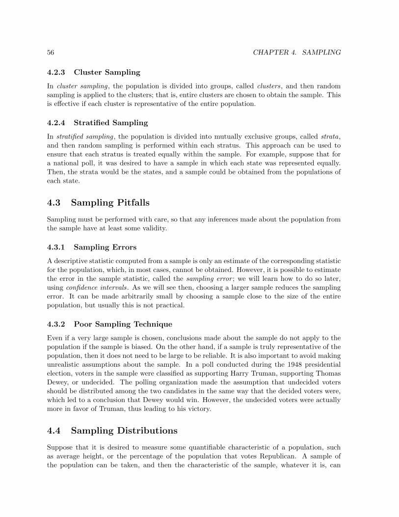
56 CHAPTER 4. SAMPLING
4.2.3 Cluster Sampling
In cluster sampling , the population is divided into groups, called clusters, and then randomsampling is applied to the clusters; that is, entire clusters are chosen to obtain the sample. Thisis effective if each cluster is representative of the entire population.
4.2.4 Stratified Sampling
In stratified sampling , the population is divided into mutually exclusive groups, called strata,and then random sampling is performed within each stratus. This approach can be used toensure that each stratus is treated equally within the sample. For example, suppose that fora national poll, it was desired to have a sample in which each state was represented equally.Then, the strata would be the states, and a sample could be obtained from the populations ofeach state.
4.3 Sampling Pitfalls
Sampling must be performed with care, so that any inferences made about the population fromthe sample have at least some validity.
4.3.1 Sampling Errors
A descriptive statistic computed from a sample is only an estimate of the corresponding statisticfor the population, which, in most cases, cannot be obtained. However, it is possible to estimatethe error in the sample statistic, called the sampling error ; we will learn how to do so later,using confidence intervals. As we will see then, choosing a larger sample reduces the samplingerror. It can be made arbitrarily small by choosing a sample close to the size of the entirepopulation, but usually this is not practical.
4.3.2 Poor Sampling Technique
Even if a very large sample is chosen, conclusions made about the sample do not apply to thepopulation if the sample is biased. On the other hand, if a sample is truly representative of thepopulation, then it does not need to be large to be reliable. It is also important to avoid makingunrealistic assumptions about the sample. In a poll conducted during the 1948 presidentialelection, voters in the sample were classified as supporting Harry Truman, supporting ThomasDewey, or undecided. The polling organization made the assumption that undecided votersshould be distributed among the two candidates in the same way that the decided voters were,which led to a conclusion that Dewey would win. However, the undecided voters were actuallymore in favor of Truman, thus leading to his victory.
4.4 Sampling Distributions
Suppose that it is desired to measure some quantifiable characteristic of a population, suchas average height, or the percentage of the population that votes Republican. A sample ofthe population can be taken, and then the characteristic of the sample, whatever it is, can

4.4. SAMPLING DISTRIBUTIONS 57
be computed from information obtained from each member of the sample. Now, suppose thatmany samples are taken, with each sample being the same size. Then, the values that arecomputed from these samples form a set of outcomes, where the experiment in question is thecomputation of the desired characteristic of the sample. This set of outcomes obtained fromsamples is called a sampling distribution.
4.4.1 Sampling Distribution of the Mean
Sampling distributions apply to a number of different statistics, but the most commonly usedis the mean. The sampling distribution of the mean is the pattern of means that is obtainedfrom computing the sample means from all possible samples of the population.
Example We will illustrate the sampling distribution of the mean for an example of rolling asix-sided die. Each of the six numbers has an equal likelihood of appearing face up, so thesevalues follow a discrete uniform probability distribution, which is a distribution that assigns thesame probability to each discrete event. Recall that the mean of such a distribution is
µ =a+ b
2,
where a and b are the minimum and maximum values, respectively, of the distribution. Thevariance is given by
σ2 =1
12[(b− a+ 1)2 − 1].
Therefore, for the case of a six-sided die, for which a = 1 and b = 6, we have µ = 3.5 andσ2 = 35/12.
Now, suppose we roll the die n times, where n is the size of our sample, and compute thesample mean x. Then, we repeat this process m times, gathering m samples, each of size n.The m sample means form a sampling distribution of the mean, which we can then display ina histogram. This is accomplished in R using the following statements (assuming the values ofn, the sample size, and m, the number of samples, are already defined):
> means=c()
> for (i in 1:m) means[i]=mean(round(runif(n,0.5,6.5)))
> hist(means,seq(1,6,0.5))
The first statement creates an empty vector called means, which will hold the sample means.The second statement executes a loop m times, in which the ith element of the means vectoris set to the mean of a vector of n numbers generated by runif from the uniform probabilitydistribution with a = 0.5 and b = 6.5, and then rounded to the nearest integer by round
to generate a sample containing numbers between 1 and 6. The third statement generates ahistogram of the frequency distribution of the sample means, with classes chosen to have width0.5.
Recall that the expression seq(a,b,h) generates a sequence of numbers starting at a andending at b, with spacing h. If the terms of the sequence have a spacing of 1, then the shorthanda:b can be used instead; note that this is used in the for statement.
Suppose we use a small sample of size n = 2, and compute m = 50 samples. The resultinghistogram is shown in Figure 4.1. The means are well-distributed across the interval from 1 to
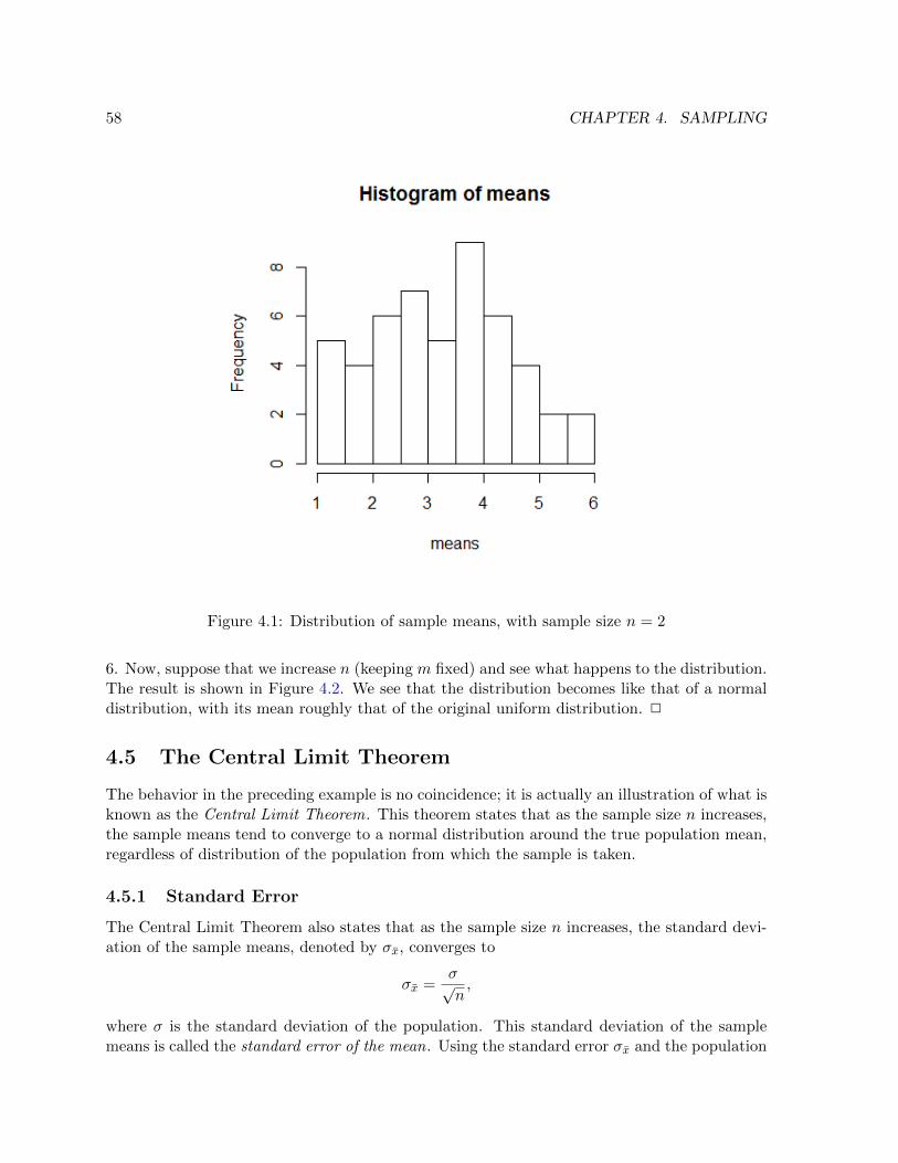
58 CHAPTER 4. SAMPLING
Figure 4.1: Distribution of sample means, with sample size n = 2
6. Now, suppose that we increase n (keeping m fixed) and see what happens to the distribution.The result is shown in Figure 4.2. We see that the distribution becomes like that of a normaldistribution, with its mean roughly that of the original uniform distribution. 2
4.5 The Central Limit Theorem
The behavior in the preceding example is no coincidence; it is actually an illustration of what isknown as the Central Limit Theorem. This theorem states that as the sample size n increases,the sample means tend to converge to a normal distribution around the true population mean,regardless of distribution of the population from which the sample is taken.
4.5.1 Standard Error
The Central Limit Theorem also states that as the sample size n increases, the standard devi-ation of the sample means, denoted by σx, converges to
σx =σ√n,
where σ is the standard deviation of the population. This standard deviation of the samplemeans is called the standard error of the mean. Using the standard error σx and the population

4.6. SAMPLING DISTRIBUTION OF THE PROPORTION 59
Figure 4.2: Distribution of sample means, with sample size n = 5 (left plot), n = 10 (centerplot), n = 20 (right plot)
mean µ, one can use the fact that the sample mean is normally distributed for sufficiently largen to compute the probability that the sample mean will fall within a certain interval, as hasbeen shown previously for a general normal distribution.
In the case of the roll of a six-sided die, with a sample size of n = 20, the standard error is
σx =σ√n
=
√35/12√
20= 0.382.
Therefore, to obtain the probability that the sample mean will be greater than 4, we computethe z-score for 4:
4− µσx
=4− 3.5
0.382= 1.309.
We conclude that
P (X > 4) = 1− P (X ≤ 4) = 1− P (Z ≤ 1.309) = 1− 0.9047 = 0.0953.
That is, there is a less than 10% chance that the sample mean will be greater than 4.
4.6 Sampling Distribution of the Proportion
In addition to the mean, we can measure the proportion of the population that possessesa characteristic that is binary in nature, such as whether a person agrees with a particularstatement. Because of the binary nature of the characteristic, the experiment of determiningits value for members of the population follows a binomial distribution. That is, the act ofinquiring of each member of the population is a Bernoulli trial, in which “success” and “failure”correspond to “yes” or “’no” responses. However, as noted previously, if the number of trials nis sufficiently large that np ≥ 5 and n(1− p) ≥ 5, where p is the probability of “success”, thenthis binomial distribution can be approximated by a normal distribution.
We therefore need the mean and standard deviation of this normal distribution. Becausethe population proportion p is unknown, we must instead use the sample proportion ps, which is

60 CHAPTER 4. SAMPLING
defined to be the number of success in the sample, divided by the sample size n. Several samplescan be taken, and then their proportion means can be averaged to obtain an approximate valuefor p. The standard deviation of this distribution, called the standard error of the proportion,is given by
σp =
√p(1− p)
n.
It is worth noting that σp is equal to the standard deviation of the binomial distribution,√np(1− p), divided by n, which makes sense because in the sampling distribution of the
proportion, we are not measuring the number of successes, as we are in the binomial distribution;rather, we are measuring the proportion of successes, thus requiring the division of both thebinomial distribution’s mean and standard deviation by n.
Example Suppose that through sampling, with samples of size n = 100, it is determined that60% of voters in California support a particular ballot initiative (that is, p = 0.6). Becausenp = 100(0.6) = 60 and n(1 − p) = 100(0.4) = 40 are large enough, we may use a normaldistribution to model the sampling distribution of the proportion. The standard error of theproportion is
σp =
√0.6(1− 0.6)
100= 0.049.
Therefore, the probability that more than 65% of the next sample will support the initiative is
P (ps > 0.65) = 1− P (ps ≤ 0.65) = 1− P (Z ≤ 1.02) = 1− 0.8461 = 0.1538,
where the z-score for 0.65 is
0.65− pσp
=0.65− 0.6
0.049= 1.02.
2
4.7 Exercises
1. The chair of the math department would like to determine the average number of daysstudents in mathematics courses are absent during the semester. He takes a sampleby gathering data on absences for 5 randomly selected students from each mathematicscourse. What type of sampling was used?
2. The time of occurrence of the first accident during rush-hour traffic at a major intersectionis uniformly distributed between the three hour interval 4 p.m. to 7 p.m. Let X = theamount of time (hours) it takes for the first accident to occur.
(a) Assume Ramon has kept track of the times for the first accidents to occur for 40 dif-ferent days. Let C = the total cumulative time. Then C follows which distribution?
A. U(0, 3)
B. Exp(13)
C. N (60, 5.477)

4.7. EXERCISES 61
D. N (1.5, 0.01875)
(b) Using the information in Exercise 2a, find the probability that the total time for allfirst accidents to occur is more than 43 hours.
3. A group of students measured the lengths of all the carrots in a five-pound bag of babycarrots. They calculated the average length of baby carrots to be 2.0 inches with astandard deviation of 0.25 inches. Suppose we randomly survey 32 five-pound bags ofbaby carrots.
(a) State the approximate distribution for Y , the distribution for the average lengths ofbaby carrots in 16 five-pound bags.
(b) Find the probability that y is between two and 2.25 inches.
4. Suppose that the time that owners keep their cars (purchased new) is normally distributedwith a mean of seven years and a standard deviation of two years. We are interested inhow long an individual keeps his car (purchased new). Our population is people who buytheir cars new.
(a) If we are to pick individuals ten at a time, find the distribution for the mean carlength ownership.
(b) If we are to pick ten individuals, find the probability that the sum of their ownershiptime is more than 55 years.

62 CHAPTER 4. SAMPLING

Chapter 5
Confidence Intervals
5.1 Introduction
Now that we have learned about sampling and sampling distributions, we are ready to learnhow to use inferential statistics to make conclusions about populations based on informationobtained from samples. A key component of inferential statistics is to quantify the uncertaintythat is inherent in using only a sample. An example of this is polling; a statement of a pollresult is accompanied by an indication of the sampling error.
5.2 Confidence Intervals for Means
Suppose that we wish to know the population mean, but only have a sample mean. We can con-struct a confidence interval that is centered at the sample mean and can provide an indicationof the population mean.
5.2.1 Large Samples
We first consider the case where the sample size n is sufficiently large, meaning that n ≥ 30.If this is the case, then, by the Central Limit Theorem, the sample means are approximatelynormally distributed, even if the population is not.
Estimators
The sample mean is an example of what is called a point estimate, which is a single value thatdescribes population. Point estimators are easy to compute, but impossible to validate. Togauge the validity of a sample mean, we will rely on an interval estimate, which is a range ofvalues that describes the population. The particular interval estimate we will use is called aconfidence interval .
Confidence Levels
The first step in constructing a confidence interval is choosing a confidence level , which is theprobability that the interval estimate will include the population parameter (in this case, the
63

64 CHAPTER 5. CONFIDENCE INTERVALS
population mean). For example, for a 90% confidence interval, the confidence level is 0.9.Subtracting this value from 1 yields the significance level α; that is, for a 90% confidenceinterval, the significance level is 0.1.
When the population standard deviation σ is known, the confidence interval is determinedas follows:
1. Compute the standard error of the mean, σx = σ/√n.
2. Find the z-value zα/2 such that for the random variable Z with standard normal distri-bution N (0, 1), P (Z ≤ zα/2) = 1− α/2, where α is the level of significance and 1− α isthe corresponding confidence level. The meaning of zα/2 is illustrated in Figure 5.1. The
Figure 5.1: Interpretation of zα/2 in terms of probability
value of zα/2 can be found by looking up the probability 1−α/2 in a normal distributiontable, or by using the R function qnorm with argument 1− α/2.
3. Compute the margin of error E = zα/2σx.
4. Then, the confidence interval is [x− E, x+ E].
Example Suppose that a signal with value µ is received with a value that is normally distributedaround µ with variance 4. To reduce error, the signal is transmitted 10 times. If the valuesreceived are 8.5, 9.5, 9.5, 7.5, 9, 8.5, 10.5, 11, 11 and 7.5, then we can construct a 95% confidenceinterval for µ as follows:

5.2. CONFIDENCE INTERVALS FOR MEANS 65
1. First, we compute the sample mean, x = 9.25.
2. Then, we compute the standard error of the mean,
σx = σ/√n = 2/
√10 = 0.6325.
3. Using α = 0.05, we obtain zα/2 = 1.96.
4. The margin of error is then
E = zα/2σx = (1.96)(0.6325) = 1.24.
5. Finally, the confidence interval is
[x− E, x+ E] = [9.25− 1.24, 9.25 + 1.24] = [8.01, 10.49].
2
Interpreting Confidence Intervals
Once the confidence interval is obtained, it is essential to interpret it correctly. Given a 90%confidence interval, it is not true that the population mean has a 90% probability of fallingwithin the interval. Instead, what we know is that there is a 90% probability that any givenconfidence interval from a random sample will contain the population mean. Note that allconfidence intervals for a given confidence level and sample size have the same width E, butthe center is the sample mean, which can vary.
Changing the Confidence Level
The significance level α represents the probability of erroneously concluding that the populationmean is outside the confidence interval, when in fact it lies within the interval. As the confidencelevel 1 − α increases, the significance level α decreases (since these two quantities must sumto one), which causes the z-score zα/2 to increase, and therefore the interval widens. As aresult, the chance of erroneously concluding that the population mean is outside the confidenceinterval decreases.
Changing the Sample Size
As the sample size n increases, the standard error of the mean decreases. It follows that themargin of error decreases, and therefore the confidence interval shrinks. This makes sensebecause with a larger sample size, the sample mean should more accurately approximate thepopulation mean.

66 CHAPTER 5. CONFIDENCE INTERVALS
Choosing the Sample Size for the Mean
Given a desired margin of error E, one can solve for the sample size n that would produce thisvalue of E for the width of the interval. Rearranging the formulas presented earlier for theconstruction of the confidence interval, we obtain
n =
(σ
σx
)2
=(σzα/2
E
)2
.
We can see from this formula that as the margin of error E decreases, the sample size n mustincrease.
When σ is Unknown
If the population standard deviation σ is unknown, a confidence interval can be obtained bysubstituting the sample standard deviation s. That is, the standard error of the mean is takento be σx = s/
√n.
5.2.2 Small Samples
When the sample size n is considered small (that is, n < 30), we can no longer rely on theCentral Limit Theorem to conclude that the sampling distribution of the mean is normal. Wemust instead assume that the population itself is normal.
When σ is Known
When the population standard deviation σ is known, then we can proceed in the same way asfor large samples.
When σ is Unknown
When σ is unknown, we can substitute s for σ as is done for large samples, but to determinethe margin of error E, instead of using the z-value zα/2 from the normal distribution, we usethe Student’s t-distribution. This distribution, like the normal distribution, is bell-shaped andsymmetric around the mean, and the area under the probability density curve is 1, but theshape of this curve depends on the degrees of freedom, which is n − 1. This is because thereare n observations in the sample, but one degree of freedom is removed due to the mean. TheStudent’s t-distribution curve is flatter than the normal distribution curve, but it converges toa normal distribution as n increases.
In this scenario, the confidence interval is given by[x− tα/2,n−1σx, x+ tα/2,n−1σx
], σx =
s√n.
The value of tα/2,n−1 can be obtained by looking up the probability 1 − α/2 in a Student’st-distribution table, or using the R function qt with arguments 1− α/2 and n− 1.
Example We revisit our previous example with a signal transmitted 10 times, except that now,the variance σ2 is unknown. Recall that the received values are 8.5, 9.5, 9.5, 7.5, 9, 8.5, 10.5, 11, 11

5.3. CONFIDENCE INTERVALS FOR PROPORTIONS 67
and 7.5. Therefore, for the standard error, we use the sample standard deviation s = 1.2964,which yields the standard error
σx =s√n
=1.2964√
10= 0.4099.
The number of degrees of freedom is n− 1 = 10− 1 = 9, and therefore we have
tα/2,n−1 = t0.05/2,9 = 2.2622
and margin of errorE = tα/2,n−1σx = 2.2622(0.4099) = 0.9274.
We conclude that the 95% confidence interval is
[x− E, x+ E] = [9.25− 0.9274, 9.25 + 0.9274] = [8.3226, 10.1774].
Note that this interval is somewhat smaller than the one constructed in the previous example,due mainly to the smaller sample standard deviation. 2
5.3 Confidence Intervals for Proportions
We will now learn how to construct confidence intervals for proportions, using the standarderror of the proportion introduced earlier. This construction is based on the approximation ofthe binomial distribution by a normal distribution, for sample size n sufficiently large so thatnp ≥ 5 and n(1 − p) ≥ 5, where p is the population proportion. If no estimate of p is known,then we use the sample proportion ps in place of p.
5.3.1 Calculating Confidence Intervals
We first compute the standard error of the proportion, except that we use the sample proportionps instead of the population proportion p:
σp =
√ps(1− ps)
n.
Then, as was done for confidence intervals for the mean, we compute zα/2, where P (Z ≤ zα/2) =1 − α/2, using either table lookup or the R function qnorm. Finally, we obtain the confidenceinterval [
ps − zα/2σp, ps + zα/2σp].
As before, the margin of error E is given by zα/2σp, which is half the width of the interval.
Example Suppose that 600 voters are polled, and 52% of them indicate that they approve ofthe president’s job performance. Using a 95% confidence interval, what is the margin of error?The standard error of the proportion, with ps = 0.52 and n = 600, is
σp =
√(0.52)(0.48)
600= 0.0204.
We also have zα/2 = z0.05/2 = 1.96. Therefore, the margin of error is
zα/2σp = 1.96(0.0204) = 0.04.
That is, the poll has a margin of error of 4%. 2
68 CHAPTER 5. CONFIDENCE INTERVALS
5.3.2 Determining the Sample Size
As with confidence intervals for the mean, we can determine the sample size n so that aconfidence level for the proportion has a given margin of error. Solving the equation for themargin of error for n yields
n =p(1− p)σ2p
=p(1− p)z2
α/2
E2.
Without an estimate of p, we can use p = 0.5 to maximize n, since that choice of p maximizesthe quantity p(1− p).
5.4 Exercises
1. Six different brands of Italian salad dressing were randomly selected at a supermarket.The grams of fat per serving are 7, 7, 9, 6, 8, 5. Assume that the underlying distributionis normal. Calculate a 95% confidence interval for the population mean grams of fat perserving of Italian salad dressing sold in supermarkets.
2. For which distribution is the median not equal to the mean?
A. Uniform
B. Exponential
C. Normal
D. Student’s t
3. Compare the standard normal distribution to the Student’s t-distribution, centered atzero. Which of the following statements are true?
A. As the number surveyed increases, the area to the left of −1 for the Student’s t-distribution approaches the area for the standard normal distribution.
B. As the degrees of freedom decrease, the graph of the Student’s t-distribution looksmore like the graph of the standard normal distribution.
C. If the number surveyed is 15, the normal distribution should never be used.
D. If the number surveyed is 40, the Student’s t-distribution yields a far more accurateconfidence interval than the normal distribution.
4. We are interested in the checking account balance of twenty-year-old college students.We randomly survey 16 twenty-year-old college students. We obtain a sample mean of$640 and a sample standard deviation of $150. Let X = checking account balance of anindividual twenty year old college student.
(a) If you were to create a confidence interval for the population mean of the checkingaccount balance of twenty-year-old college students, what distribution would youuse?
(b) Find the 95% confidence interval for the true mean checking account balance of atwenty-year-old college student.
5.4. EXERCISES 69
5. A recent survey of U.S. teenage pregnancy was answered by 720 girls, age 12-19. Sixpercent of the girls surveyed said they have been pregnant. We are interested in the trueproportion of U.S. girls, age 12-19, who have been pregnant.
(a) Find the 95% confidence interval for the true proportion of U.S. girls, age 12-19, whohave been pregnant.
(b) The report also stated that the results of the survey are accurate to within ±3.7%at the 95% confidence level. Suppose that a new study is to be done. It is desired tobe accurate to within 2% of the 95% confidence level. What is the minimum numberthat should be surveyed?
6. You draw a sample of size 30 from a normally distributed population with a standarddeviation of four.
(a) What is the standard error of the sample mean in this scenario, rounded to twodecimal places?
(b) What is the distribution of the sample mean?
(c) If you want to construct a two-sided 95% confidence interval, how much probabilitywill be in each tail of the distribution?
(d) What is the appropriate error bound or margin of error (E) for a 95% confidenceinterval for this data?
(e) Rounding to two decimal places, what is the 95% confidence interval if the samplemean is 41?
(f) What is the 90% confidence interval if the sample mean is 41? Round to two decimalplaces
(g) Suppose the sample size in this study had been 50, rather than 30. What would the95% confidence interval be if the sample mean is 41? Round your answer to twodecimal places.
7. For any given data set and sampling situation, is a 95% confidence interval wider than a99% confidence interval?

70 CHAPTER 5. CONFIDENCE INTERVALS

Chapter 6
Hypothesis Testing
In this chapter, we explore one of the most useful applications of inferential statistics, that trulydemonstrates its power: hypothesis testing , in which a sample is used to determine, within acertain level of confidence, whether to reject a hypothesis about the population from which thesample was drawn. This is a prime example of how statistics is useful for acquiring insight intopopulations from raw data.
6.1 Introduction
A hypothesis is defined to be an assumption about a population parameter. In this chapter, wewill formulate hypotheses about whether a certain parameter is less than, equal to, or greaterthan a certain value, and then use confidence intervals to test whether these hypotheses shouldbe rejected.
6.1.1 The Null and Alternative Hypotheses
For hypothesis testing, we use two hypotheses:
• The null hypothesis, denoted by H0, represents the “status quo”. It states a belief abouthow a population parameter, such as the mean or a proportion, compares to a specificvalue.
• The alternative hypothesis, denoted by H1, is the opposite of H0.
6.1.2 Stating the Null and Alternative Hypotheses
For hypothesis testing to be as useful as possible, it is important to choose the alternativehypothesis H1 wisely. The alternative hypothesis plays the role of the “research hypothesis”;that is, it corresponds to the position that the researcher wants to establish.
Example Suppose that a brand of lightbulbs has a mean lifetime of 2000 hours, but an im-provement has been made to their design that may extend their lifetime. Then, an appropriatenull hypothesis for this situation would be H0 : µ ≤ 2000, and the corresponding alternativehypothesis would be H1 : µ > 2000. Therefore, if it is determined that H0 should be rejected,
71
72 CHAPTER 6. HYPOTHESIS TESTING
then there is evidence to support the claim that the newly designed lightbulbs do in fact havea longer lifetime. 2
6.2 Type I and Type II Errors
The way a hypothesis test proceeds as follows: first, we determine a rejection region of thesampling distribution for the parameter featured in H0 (for example, the sampling distributionof the mean). Then, we check whether an appropriate test statistic (for example, the samplemean) falls within the rejection region. If so, we choose to reject H0, and conclude that there issufficient evidence support the claim made by H1. Otherwise, we choose not to reject H0, andconclude that there is not sufficient evidence to support the claim made by H1. It’s importantto note that a hypothesis test does not provide enough evidence to accept H0; we are onlyconcerned with whether to reject it.
Because of the reliance on a sample, it is possible for the conclusion of a hypothesis test tobe erroneous. There are two kinds of erroneous conclusions:
• A Type I error is committed when the decision is made to reject H0, even though it isactually valid. This kind of error is often due to a sampling error. The probability of aType I error is the level of significance used to construct the confidence interval used forthe hypothesis test; as before, this probability is denoted by α.
• A Type II error is committed when the decision is made not to reject H0 even though itis actually false. The probability of such an error is denoted by β.
For a fixed sample size, β decreases as α increases. However, the probability of both errors canbe decreased by increasing the sample size.
6.3 Two-Tail Hypothesis Testing
A two-tail hypothesis test is a hypothesis test in which the null hypothesis H0 is a statementof equality. For example, a null hypothesis for the mean would be of the form H0 : µ = µ0, forsome chosen value of µ0.
We first choose the significance level α, based on what is considered an acceptable probabilityof making a Type I error. Then, we construct a confidence interval around µ0, which, as learnedin the previous chapter, is
[µ0 − zα/2σx, µ0 + zα/2σx].
If the sample mean x falls within this confidence interval, then we do not reject H0. Otherwise,we say that x falls within the rejection region (that is, the subset of the real number line outsideof the confidence interval), and we reject H0.
By rearranging algebraically, we obtain the equivalent condition that we do not reject H0
if the test statistic
z∗ =x− µ0
σx
satisfies
−zα/2 ≤ z∗ ≤ zα/2.

6.4. ONE-TAIL HYPOTHESIS TESTING 73
6.4 One-Tail Hypothesis Testing
A one-tail hypothesis test is a hypothesis test in which the null hypothesis H0 is an inequality.For example, a null hypothesis for the mean would be of the form H0 : µ ≤ µ0 or H0 : µ ≥ µ0.
As with the two-tail test, we first choose the significance level α. Then, we construct aone-sided confidence interval. For the null hypothesis H0 : µ ≤ µ0, the interval is
(−∞, µ0 + zασx].
If the sample mean x falls within this confidence interval (that is, x ≤ µ0 + zασx), then we donot reject H0. Otherwise, if x > µ0 + zασx, then x falls within the rejection region, and wereject H0. Equivalently, we do not reject H0 if the sample mean satisfies
z∗ ≤ zα.
Similarly, if the null hypothesis is H0 : µ ≥ µ0, we do not reject H0 if
z∗ ≥ −zα.
Note that one-tail hypothesis testing uses the same test statistic as in the two-tail case, but itis compared to different values.
6.5 Hypothesis Testing with One Sample
We now consider hypothesis testing in several scenarios, all of which involve only one sample.In each scenario, the general idea is the same: a confidence interval needs to be constructedaround the value that is compared to the parameter in H0. Outside this interval lies therejection region; if the test statistic falls within the rejection region, then H0 is rejected. Thedifferences between scenarios relate to the various parameters used to construct the confidenceinterval.
6.5.1 Testing for the Mean, Large Sample
First, we consider hypothesis testing for the case in which the parameter of interest is the mean,and the sample is large (that is, of size 30 or more). Under this assumption, by the Central LimitTheorem, the sampling distribution of the mean is well approximated by a normal distribution.We will consider both one-tail hypothesis tests, for which the null hypothesis is of the formH0 : µ ≥ µ0 or H0 : µ ≤ µ0, and two-tail tests, for which the null hypothesis is of the formH0 : µ = µ0.
When σ is Known
When the population standard deviation σ is known, then the appropriate test statistic is theone introduced in the preceding discussion,
z∗ =x− µ0
σx,

74 CHAPTER 6. HYPOTHESIS TESTING
where σx = σ/√n is the standard error of the mean.
Example A commercial hatchery grows salmon whose weights are normally distributed witha standard deviation of 1.2 pounds. The hatchery claims that the mean weight is at least 7.6pounds. Suppose a random sample of 40 fish yields an average weight of 7.2 pounds. Is thisstrong enough evidence to reject the hatchery’s claim at the 5% level of significance?
We use the null hypothesis H0 : µ ≥ 7.6, and alternative hypothesis H1 : µ < 7.6. Thestandard error is
σx =σ√n
=1.2√40
= 0.1897.
The test statistic is
z∗ =x− µ0
σx=
7.2− 7.6
0.1897= −2.1082.
We then compare this value to −zα = −z0.05 = −1.6449. Because z∗ < −zα, the test statisticfalls within the rejection region, and therefore we reject H0 and conclude that the hatchery’sclaim does not have merit. 2
When σ is Unknown
By contrast, when σ is unknown, we substitute s, the sample standard deviation, for σ andproceed as before. Because the sample is large, it is assumed that s is a reasonably accurateapproximation for σ. Therefore, the test statistic is
z∗ =x− µ0
s/√n.
Example Twenty years ago, male students at a high school could do an average of 24 pushupsin 60 seconds. To determine whether this is still true today, a sample of 50 male students waschosen. If the sample mean was 22.5 pushups and the sample standard deviation was 3.1, canwe conclude that the mean is no longer 24?
Our null hypothesis is H0 : µ = 24, and the alternative hypothesis is H1 : µ 6= 24. We testat the 5% level of significance. Since the population standard deviation is unknown, but thesample is sufficiently large, we use the sample standard deviation instead. Then, the standarderror is
σx =s√n
=3.1√50
= 0.4384,
and the test statistic is
z∗ =x− µ0
σx=
22.5− 24
0.4384= −3.4215.
Because this is a two-tail test, we compare z∗ to zα/2 = z0.025 = 1.96. We have |z∗| > zα/2,which means z∗ falls within the rejection region. Therefore, we reject H0 and conclude that themean is no longer 24. 2
6.5. HYPOTHESIS TESTING WITH ONE SAMPLE 75
6.5.2 The Role of α
It can be seen from examination of a normal distribution table that as α increases, zα (or zα/2,for that matter) decreases, because zα is the z-value for which P (Z > zα) = α, or, equivalently,P (Z ≤ zα) = 1− α. It follows that the test statistic is less likely to fall within the appropriateconfidence interval for the hypothesis test; that is, it is more likely that H0 will be rejected.
Considering that the alternative hypothesis H1 is generally the one that supports a positionthat a researcher is trying to establish, it is in the researcher’s interest that H0 be rejected.As such, they can help their cause by choosing a larger value of α, which corresponds to alower confidence level 1 − α. This is an important ethical consideration for a statistician, andunderscores the importance of knowing the parameters used in any statistical analysis that isused to support a particular position. The smaller the value of α, the more confidence (punintended) one can have in the result of a hypothesis test.
6.5.3 p-Values
Since it is important to avoid a Type I error (rejecting H0 when it is actually valid), and theprobability of making this error is the level of significance α, it is helpful to have some guidancein choosing α. For this reason, we introduce the concept of a p-value, which is defined to bethe smallest value of significance at which H0 will be rejected, assuming it is true.
One-Tail Tests
Recall that for a one-tail test of a hypothesis of the formH0 : µ ≤ µ0, with alternative hypothesisH1 : µ > µ0, H0 should be rejected if
z∗ > zα.
Because zα satisfies P (Z > zα) = α, it follows that H0 will be rejected if
P (Z > z∗) < α.
We therefore take the p-value for such a hypothesis test to be
P (Z > z∗) .
This is illustrated in Figure 6.1. On the other hand, if the null hypothesis is H0 : µ ≥ µ0, thenH0 is rejected if
z∗ < −zα.
Because P (Z ≤ −zα) = α, it follows that H0 is to be rejected if
P (Z ≤ z∗) < α.
We conclude that the p-value is P (Z ≤ z∗).

76 CHAPTER 6. HYPOTHESIS TESTING
Figure 6.1: Rejection region and p-value for a one-tail hypothesis test
Two-Tail Tests
The determination of a p-value for a two-tail test is similar to the one-tail case. For such a test,the null hypothesis H0 : µ = µ0 is rejected if
|z∗| > zα/2.
Because zα/2 satisfies P (|Z| > zα/2) = α, it follows that H0 is rejected if
P (|Z| > |z∗|) < α.
Due to the symmetry of the normal distribution, this condition is equivalent to
P (Z > |z∗|) < α/2.
That is, the p-value for a two-tail test is twice the p-value of the corresponding one-tail test.
6.5.4 Testing for the Mean, Small Sample
When the sample size is small (that is, less than 30), we can no longer rely on the CentralLimit Theorem and automatically treat the sampling distribution of the mean as a normaldistribution.

6.5. HYPOTHESIS TESTING WITH ONE SAMPLE 77
When σ is Known
When the population standard deviation σ is known, then we can proceed with hypothesistesting as before, provided that the population is in fact normally distributed. If this is not thecase, then the result of a hypothesis test may be unreliable.
When σ is Unknown
When σ is unknown, but it can be assumed that the population is normally distributed, thenwe need an alternative approach to computing the threshold against which to compare the teststatistic (that is, the value that plays the role of zα in a one-tail test or zα/2 in a two-tailtest). For this purpose, we use the Student’s t-distribution, as we did before when constructingconfidence intervals using small samples with σ unknown. As in the case of a large sample withσ unknown, our test statistic is
t∗ =x− µ0
s/√n.
This test statistic is compared to a value of the Student’s t-distribution with n − 1 degrees offreedom, where n is the sample size. For a given significance level α, we let tα,n−1 be the t-valuesuch that P (Tn−1 > tα,n−1) = α, where Tn−1 is a random variable that follows the Student’st-distribution with n− 1 degrees of freedom.
For a one-tail test, with null hypothesis H0 : µ ≤ µ0, we reject H0 if t∗ > tα,n−1, and do notreject H0 otherwise. On the other hand, if the null hypothesis is H0 : µ ≥ µ0, we reject H0 ift∗ < −tα,n−1, and do not reject H0 otherwise. Finally, for a two-tail test with null hypothesisH0 : µ = µ0, we reject H0 if |t∗| > tα/2,n−1, and do not reject H0 if |t∗| ≤ tα/2,n−1.
6.5.5 Testing for the Proportion, Large Samples
We now consider hypothesis testing for a different population parameter, a proportion. Since theproportion follows a binomial distribution, we must use the binomial distribution to computethe test statistic and p-value if the sample size n is small. However, if n is large, then thebinomial distribution is well-approximated by a normal distribution, which we assume in thefollowing discussion.
One-Tail Test
We first consider a one-tail test for the proportion, in which the null hypothesis is of the formH0 : p ≤ p0, and the alternative hypothesis is H1 : p > p0. The test statistic for this kind oftest is
z∗ =p− p0
σp,
where σp is the standard error of the proportion, given by
σp =
√p0(1− p0)
n.
We then reject H0 if z∗ > zα. Similarly, if the null hypothesis is H0 : p ≥ p0, we reject H0 ifz∗ < −zα.

78 CHAPTER 6. HYPOTHESIS TESTING
Two-Tail Test
For a two-tail test with null hypothesis H0 : p = p0, and alternative hypothesis H1 : p 6= p0, weuse the same test statistic z∗ as in the one-tail case, and reject H0 if |z∗| > zα/2.
6.5.6 Writing Functions in R
To illustrate how to write a function in R, we build a function that performs two-tail hypothesistesting for the mean in the case of an unknown variance (large or small sample). As such, thefunction will need this information:
1. The data from the sample, x1, x2, . . . , xn
2. The value µ0 in the null hypothesis H0 : µ = µ0
3. The level of significance α
The code follows:
## 2-tail hypothesis test of mean, variance unknown
meantest2tail <- function(x,mu0,alpha) {
## sample mean
xbar=mean(x)
## sample standard deviation
s=sd(x)
## standard error
n=length(x)
stderr=s/sqrt(n)
## test statistic
teststat=(xbar-mu0)/stderr
if ( n < 30 )
## small sample: p-value from Student’s t-distribution
pval=2*(1-pt(abs(teststat),df=n-1))
else
## large sample: use normal distribution
pval=2*(1-pnorm(abs(teststat)))
## perform test
if (alpha>pval)
result="reject H0"
else
result="do not reject H0"
## return results
list(TestStatistic=teststat,pValue=pval,Conclusion=result)
}
This code should be typed into a file named meantest2tail.R. Then, it is loaded into the Rworkspace using the source command:
> source("meantest2tail.R")
6.6. HYPOTHESIS TESTING WITH TWO SAMPLES 79
The filename needs to be in R’s search path; otherwise, a full pathname must be used. If thecode is revised, then the source command must be used again in order to load the latest versionof the code.
The code above associates the function expression with the name meantest2tail forfuture use. The list after the function keyword specifies the input parameters that this functionexpects. Then, the code computes the sample mean, sample standard deviation, standard error,and test statistic, according to the discussion earlier in this section. Next, the appropriate p-value is computed, according to whether the sample size is considered large (which calls for thenormal distribution z-value zα/2) or small (which calls for the Student’s t-distribution t-valuetα/2,n−1).
Finally, the p-value is compared to the level of significance and a list of named outputvalues is constructed. The list contains three elements, named TestStatistic, pValue, andConclusion. The result of this expression is returned by the function when it is called. Wenow illustrate the usage of our function, by reading the age data from Chapter 1 and testingthe null hypothesis H0 : µ = 50 with significance level 0.1.
> x=scan("ages.txt")
Read 100 items
> hyptest=meantest2tail(x,50,0.1)
> hyptest$Conclusion
[1] "do not reject H0"
> hyptest[["pValue"]]
[1] 0.1572436
The named list constructed in the last statement of the function body is stored in the variablehyptest. Then, the elements of the list can be accessed using their names. Note that in theabove statements, two different conventions are used to access these elements.
6.6 Hypothesis Testing with Two Samples
We now consider testing hypotheses involving characteristics of two populations. Examples ofsituations that call for a two-sample test include
• investigating differences in test scores between males and females,
• comparison of long-life vs standard light bulbs, and
• average selling prices of homes in different areas.
6.6.1 Sampling Distribution for the Difference of Means
Two-sample hypothesis testing can be used to compare means. For this purpose, we use thesampling distribution for the difference in means, which describes the probability of observingvarious intervals for difference between two sample means. To perform hypothesis testing withthis distribution, we need the standard error of the difference,
σx1−x2 =
√σ2
1
n1+σ2
2
n2, (6.1)
80 CHAPTER 6. HYPOTHESIS TESTING
where the first sample of size n1 has standard deviation σ1, and the second sample of size n2
has standard deviation σ2.
6.6.2 Testing for Difference of Means, Large Samples
If the sample sizes n1 and n2 are large, then it can be assumed that the sampling distributionof the difference of means follows a normal distribution. The test statistic is then
z∗ =x1 − x2
σx1−x2,
where σx1−x2 is defined in (6.1). For this discussion, we need to assume that the two samplesare independent of one another.
Example Two new methods of producing a tire are to be compared. For the first method,n1 = 40 tires are tested at location A and found to have a mean lifetime of x1 = 40, 000 miles,while for the second method, n2 = 50 tires are tested at location B and found to have a meanlifetime of x2 = 42, 000 miles. It is known that tires tested at location A have a standarddeviation of σ1 = 4, 000 miles, while tires tested at location B have a standard deviation ofσ2 = 5, 000 miles. We wish to test the hypothesis that both methods produce tires with thesame average lifetimes.
The null hypothesis is H0 : µ1 = µ2, and the alternative hypothesis is H1 : µ1 6= µ2. Wetest at the 5% significance level. The standard error is
σx1−x2 =
√σ2
1
n1+σ2
2
n2=
√40002
40+
50002
50= 948.6833.
Then, the test statistic is
z∗ =x1 − x2
σx1−x2=
40, 000− 42, 000
948.6833= −2.1082.
We compare this against zα/2 = z0.05/2 = 1.96. Since |z∗| > zα/2, we reject the null hypothesisand conclude that the two methods produce tires with statistically different average lifetimes.
It is worth noting that the p-value is
P (|Z| > | − 2.1082|) = 2P (Z > 2.1082) = 2(1− P (Z ≤ 2.1082)) = 0.035.
That is, the null hypothesis would be rejected at any significance level above 3.5%. 2
6.6.3 Testing for Difference of Means, Unknown Variance
If the standard deviations are unknown, then we must use the Student’s t-distribution. Whenthe sample sizes are small (that is, n1, n2 < 30) we must assume that the populations arenormally distributed. For now, we assume that the samples are independent; this kind ofhypothesis test is called an unpaired t-test.

6.6. HYPOTHESIS TESTING WITH TWO SAMPLES 81
Equal Standard Deviations
When the population standard deviations are unknown but assumed to be equal, we use thesample standard deviations to obtain a pooled estimate of standard deviation:
sp =
√(n1 − 1)s2
1 + (n2 − 1)s22
n1 + n2 − 2
Note that the degrees of freedom of the samples, n1 − 1 and n2 − 1, are added to obtain thedegrees of freedom to be used for the test, n1 + n2 − 2.
We then obtain the standard error of the difference of means as follows:
σx1−x2 = sp
√1
n1+
1
n2
The corresponding test statistic is
t∗ =d− d0
σd,
where, for conciseness, the variable d represents x1 − x2, and d0 is the value of d against whichwe are testing.
Unequal Standard Deviations
When the standard deviations are unequal, we perform an unpooled test. We first define thestandard error of the difference of means as
σx1−x2 =
√s2
1
n1+s2
2
n2.
In this case, we define the number of degrees of freedom by
d.f. =
(s2
1
n1+s2
2
n2
)2
(s21n1
)2
n1 − 1+
(s22n2
)2
n2 − 1
,
which must be rounded to an integer.
Testing for Difference of Means, Dependent Samples
Now, suppose that the two samples are actually dependent on one another. An example wouldbe testing the average weight loss of a group of individuals, in which each person’s original weightmust be paired with their current weight. In this situation, we use the Student’s t-distributionfor what is called a paired t-test .
Example Suppose that a group of 10 patients is given medication that is intended to lowertheir cholesterol. Their cholesterol is tested before and after being given the medication, and

82 CHAPTER 6. HYPOTHESIS TESTING
they are found to have their cholesterol level lowered by an average of d = 10 mg/dL, witha sample standard deviation of sd = 8 mg/dL. If we test at the 1% significance level, is thereduction in cholesterol level statistically significant?
Our null hypothesis is that the medication does not help; that is, H0 : µ ≤ 0, where µ is themean reduction in cholesterol level. The alternative hypothesis is H1 : µ > 0. The standarderror is
σd =sd√n
=8√10
= 2.5298.
Then, the test statistic is
t∗ =d− 0
σd=
10
2.5298= 3.9528.
We compare this value to tα,n−1 = t0.01,9 = 2.8214. Because t∗ > tα,n−1, we reject H0 andconclude that the reduction in cholesterol level is statistically significant. 2
6.6.4 Testing for Difference of Proportions
We now consider testing for the difference of proportions. As in the one-sample case, we assumethat the sample sizes are large enough to allow approximation of the binomial distributionsfollowed by the variables X1 and X2 to be approximated by normal distributions.
Let p1 and p2 be the true proportions of the two populations, and let p1 and p2 be thesample proportions from samples of size n1 and n2, respectively. If the null hypothesis isH0 : p1 = p2, then we use this assumption of equality to compute the following estimate of theoverall proportion of the two populations:
p =n1p1 + n2p2
n1 + n2,
Then, the standard error of the proportion is
σp1−p2 =
√p(1− p)
(1
n1+
1
n2
).
On the other hand, if the null hypothesis is H0 : p1 − p2 = d0 for some nonzero value d0,then we use the standard error
σp1−p2 =
√p1(1− p1)
n1+p2(1− p2)
n2.
In either case, we use the test statistic
z∗ =(p1 − p2)− d0
σp1−p2,
where we assume d0 = 0 in the case of the null hypothesis H0 : p1 = p2.

6.7. SUMMARY 83
6.7 Summary
As we have seen, there are several hypothesis tests for different situations, and various ways toconduct the test that are all mathematically equivalent. To help keep track of these situations,the following principles can be applied:
• The test statistic is always the difference between the value of the variable being tested(e.g. the sample mean) and the value it’s being tested against (e.g. µ0 if the null hypothesisis H0 : µ = µ0), divided by the standard error.
• We use the Student’s t-distribution if the variances are unknown. In this case, we usesample standard deviations to obtain the standard error.
We summarize the standard errors for various scenarios in Table 6.1.
Characteristic Scenario Standard Error
µ Variance known σx = σ/√n
µ Variance unknown σx = s/√n
p n sample σp =
√p0(1− p0)
n
µ1 − µ2 ni large, σi known, σx1−x2 =
√σ2
1
n1+σ2
2
n2
independent samples
µ1 − µ2 ni large, σi unknown, σx1−x2 = sp
√1
n1+
1
n2,
σ1 = σ2, independent sp =
√(n1 − 1)s2
1 + (n2 − 1)s22
n1 + n2 − 2
µ1 − µ2 ni large, σi unknown, σx1−x2 =
√s2
1
n1+s2
2
n2,
σ1 6= σ2, independent
d = µ1 − µ2 n large, σ unknown, σd = sd/√n
dependent samples
p1 − p2 ni large, H0 : p1 = p2 σp1−p2 =
√p(1− p)
(1
n1+
1
n2
),
p =n1p1 + n2p2
n1 + n2
p1 − p2 ni large, H0 : p1 − p2 = d σp1−p2 =
√p1(1− p1)
n1+p2(1− p2)
n2
Table 6.1: Standard error for various hypothesis tests
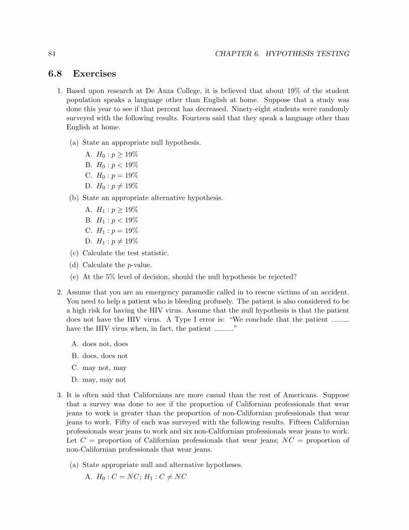
84 CHAPTER 6. HYPOTHESIS TESTING
6.8 Exercises
1. Based upon research at De Anza College, it is believed that about 19% of the studentpopulation speaks a language other than English at home. Suppose that a study wasdone this year to see if that percent has decreased. Ninety-eight students were randomlysurveyed with the following results. Fourteen said that they speak a language other thanEnglish at home.
(a) State an appropriate null hypothesis.
A. H0 : p ≥ 19%
B. H0 : p < 19%
C. H0 : p = 19%
D. H0 : p 6= 19%
(b) State an appropriate alternative hypothesis.
A. H1 : p ≥ 19%
B. H1 : p < 19%
C. H1 : p = 19%
D. H1 : p 6= 19%
(c) Calculate the test statistic.
(d) Calculate the p-value.
(e) At the 5% level of decision, should the null hypothesis be rejected?
2. Assume that you are an emergency paramedic called in to rescue victims of an accident.You need to help a patient who is bleeding profusely. The patient is also considered to bea high risk for having the HIV virus. Assume that the null hypothesis is that the patientdoes not have the HIV virus. A Type I error is: “We conclude that the patienthave the HIV virus when, in fact, the patient .”
A. does not, does
B. does, does not
C. may not, may
D. may, may not
3. It is often said that Californians are more casual than the rest of Americans. Supposethat a survey was done to see if the proportion of Californian professionals that wearjeans to work is greater than the proportion of non-Californian professionals that wearjeans to work. Fifty of each was surveyed with the following results. Fifteen Californianprofessionals wear jeans to work and six non-Californian professionals wear jeans to work.Let C = proportion of Californian professionals that wear jeans; NC = proportion ofnon-Californian professionals that wear jeans.
(a) State appropriate null and alternative hypotheses.
A. H0 : C = NC; H1 : C 6= NC
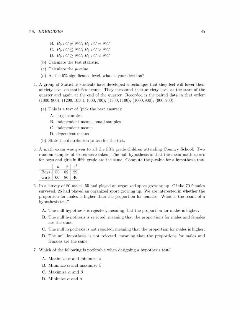
6.8. EXERCISES 85
B. H0 : C 6= NC; H1 : C = NC
C. H0 : C ≤ NC; H1 : C > NC
D. H0 : C ≥ NC; H1 : C < NC
(b) Calculate the test statistic.
(c) Calculate the p-value.
(d) At the 5% significance level, what is your decision?
4. A group of Statistics students have developed a technique that they feel will lower theiranxiety level on statistics exams. They measured their anxiety level at the start of thequarter and again at the end of the quarter. Recorded is the paired data in that order:(1000, 900); (1200, 1050); (600, 700); (1300, 1100); (1000, 900); (900, 900).
(a) This is a test of (pick the best answer):
A. large samples
B. independent means, small samples
C. independent means
D. dependent means
(b) State the distribution to use for the test.
5. A math exam was given to all the fifth grade children attending Country School. Tworandom samples of scores were taken. The null hypothesis is that the mean math scoresfor boys and girls in fifth grade are the same. Compute the p-value for a hypothesis test.
n x s2
Boys 55 82 29Girls 60 86 46
6. In a survey of 80 males, 55 had played an organized sport growing up. Of the 70 femalessurveyed, 25 had played an organized sport growing up. We are interested in whether theproportion for males is higher than the proportion for females. What is the result of ahypothesis test?
A. The null hypothesis is rejected, meaning that the proportion for males is higher.
B. The null hypothesis is rejected, meaning that the proportions for males and femalesare the same.
C. The null hypothesis is not rejected, meaning that the proportion for males is higher.
D. The null hypothesis is not rejected, meaning that the proportions for males andfemales are the same.
7. Which of the following is preferable when designing a hypothesis test?
A. Maximize α and minimize β
B. Minimize α and maximize β
C. Maximize α and β
D. Minimize α and β

86 CHAPTER 6. HYPOTHESIS TESTING
8. Consider the following claim: “The average adult drinks 3.1 cups of coffee per day.” Statethe null hypothesis H0 and alternative hypothesis H1 for this claim. A sample of 40 adultsdrank an average of 3.3 cups per day. Assume the population standard deviation is 0.5cups. Test your hypothesis using a significance level of α = 0.5 and state your conclusion.
9. Test the claim that the average gasoline consumption per car in the United States isat least 1.8 gallons per day, with a population standard deviation of 0.9. Assume thepopulation is normally distributed. A sample of 30 cars yields a sample mean of 1.5gallons. Use α = 0.05. What is the p-value for this sample?

Chapter 7
The Chi-Square Distribution
In this chapter, we will use hypothesis testing for new purposes:
• To determine whether a given data set follows a specific probability distribution, and
• To determine whether two random variables are statistically independent.
7.1 Review of Data Measurement Scales
Recall from Chapter 1 that there are four data measurement scales: nominal, ordinal, interval,and ratio. The hypothesis testing techniques presented in Chapter 6 only apply to the scales thatare more quantitative, interval and ratio. Now, though, we can use hypothesis testing for datameasured in nominal or ordinal scales as well. This is because we are working with frequencydistributions, which can be constructed from any data set, regardless of its measurement scale.
7.2 The Chi-Square Goodness-of-Fit Test
The chi-square goodness-of-fit test uses a sample to determine whether the frequency distribu-tion of the population conforms to a particular probability distribution that it is believed tofollow.
Example Suppose that a six-sided die is rolled 150 times, and the result of each roll is recorded.The number of rolls that are a 1,2,3, 4,5 or 6 should follow a uniform distribution. A chi-squaregoodness-of-fit test can be used to compare the observed number of rolls for each value, from 1to 6, to the expected number of rolls for each value, which is 150/6 = 25. 2
7.2.1 Stating the Hypotheses
For the chi-square goodness-of-fit test, the null hypothesis H0 is that the population does followthe predicted distribution, and the alternative hypothesis H1 is that it does not.
7.2.2 Observed and Expected Frequencies
The chi-square goodness-of-fit test works with two frequency distributions, with the sameclasses, and frequencies denoted by {Oi} and {Ei}, respectively. Each frequency Oi is the
87

88 CHAPTER 7. THE CHI-SQUARE DISTRIBUTION
actual number of observations from the sample that belong to the ith class. Each frequency Eiis the expected number of observations that should belong to class i, assuming H0 is true. It isessential that the total number of observations in both frequency distributions are equal; thatis,
n∑i=1
Oi =
n∑i=1
Ei,
where n is the number of classes.
7.2.3 Calculating the Chi-Square Statistic
The test statistic for the chi-square goodness-of-fit test, also known as the chi-square score isgiven by
χ2 =n∑i=1
(Oi − Ei)2
Ei,
where, as before, n is the number of classes.
7.2.4 Determining the Critical Chi-Square Score
Once we have computed the test statistic, we compare it against the critical value χ2c , which
can be obtained as follows:
• It can be looked up in a table of right-tail areas for the chi-square distribution, with thedegrees of freedom d.f. = n− 1 and chosen significance level α, or
• One can use the R function qchisq with first parameter 1 − α and second parameterd.f. = n−1; this function returns the left-tail area corresponding to these parameters,in contrast to the table given in Appendix A, which is why 1 − α is given as the firstparameter instead of α.
If the chi-square score χ2 is greater than this critical value χ2c , then we reject H0; otherwise we
do not reject H0. It should be noted that because test statistic and critical value are alwayspositive, the chi-square goodness of fit test is always a one-tail test.
7.2.5 Characteristics of a Chi-Square Distribution
The chi-square distribution is of a very different character than other distributions that we haveseen. If Z1, Z2, . . . , Zn are independent, standard random normal variables, then the randomvariable Q defined by
Q =n∑i=1
Z2i
follows the chi-square distribution with n degrees of freedom.It is not symmetric; rather, its values are skewed toward zero, which is the leftmost value of
the distribution. However, as the number of degrees of freedom (d.f.) increases, the distributionbecomes more symmetric. The probability density function for this distribution is
fn(x) =1
2n/2Γ(n/2)xn/2−1e−x/2,

7.2. THE CHI-SQUARE GOODNESS-OF-FIT TEST 89
where n is the number of degrees of freedom and Γ(n) is the gamma function, which happensto be an extension of the factorial function to the real numbers (that is, Γ(n) = (n − 1)! if nis a positive integer). The probability distribution, which is the graph of fn(x), is shown forvarious values of n in Figure 7.1.
Figure 7.1: The chi-square distribution for various values of df , the degrees of freedom
7.2.6 A Goodness-of-Fit Test with the Binomial Distribution
Suppose a coin is flipped 10 times, and the number of times it comes up heads is recorded.Then, this process is repeated several times, for a total of 100 sequences of 10 flips each. Thetable below reports how many sequences produced k heads, for k = 0, 1, 2, . . . , 10. Since coinflips are Bernoulli trials, the number of heads follows a binomial distribution, so the table alsoreports the expected number of sequences that produces k heads.
Number of heads Observed Sequences Expected Sequences
0 1 0.0981 2 0.9772 3 4.3953 9 11.7184 18 20.5075 26 24.6106 21 20.5077 13 11.7188 5 4.3959 2 0.97710 0 0.098

90 CHAPTER 7. THE CHI-SQUARE DISTRIBUTION
Our null hypothesis H0 is that the number of heads does in fact follow a binomial distribution.The chi-square score is
χ2 =
10∑i=1
(Oi − Ei)2
Ei
=(1− 0.098)2
0.098+
(2− 0.977)2
0.977+
(3− 4.395)2
4.395+
(9− 11.718)2
11.718+
(18− 20.507)2
20.507+
(26− 24.610)2
24.610+
(21− 20.507)2
20.507+
(13− 11.718)2
11.718+
(5− 4.395)2
4.395+
(2− 0.977)2
0.977+
(0− 0.098)2
0.098= 12.236.
This is compared to the critical value χ2c , with degrees of freedom d.f. = n − 1 = 10, since
there are n = 11 classes, with level of significance α = 0.05. We use the R expressionqchisq(1-0.05,10) to obtain χ2
c = 18.307. Since χ2 < χ2c , we do not reject H0, and con-
clude that the distribution of the number of heads from each sequence of 10 flips follows abinomial distribution, as expected. 2
7.3 Chi-Square Test for Independence
Now, we use the chi-square distribution to test whether two given random variables are statis-tically independent. For this test, the null hypothesis H0 is that the variables are independent,while the alternative hypothesis H1 is that they are not.
To compute the test statistic, we construct a contingency table, which is a two-dimensionalarray, or a matrix, in which each cell contains an observed frequency of an ordered pair of valuesof the two variables. That is, the entry in row i, column j, which we denote by Oi,j , containsthe number of observations that fall into class i of the first variable and class j of the second.The frequencies in this table are the observed frequencies for the chi-square goodness of fit test.
Next, for each row i and each column j, we compute Ei,j , which is the sum of the entriesin row i times sum of the entries of column j, divided by the total number of observations, toget the expected frequencies for the chi-square goodness-of-fit test. That is, if the contingencytable has m rows and n columns, then
Ei,j =
(n∑k=1
Oi,k
)(m∑`=1
O`,j
)∑m
`=1
∑nk=1O`,k
.
It should be noted that this quantity, divided again by the total number of observations, isexactly P (Ai)P (Bj), where Ai is the event that the first variable falls into class i, and Bj isthe event that the second variable falls into class j. By the multiplication rule, this probabilitywould equal P (Ai ∩Bj) if the variables were independent.
Then, the test statistic is
χ2 =m∑i=1
n∑j=1
(Oi,j − Ei,j)2
Ei,j.
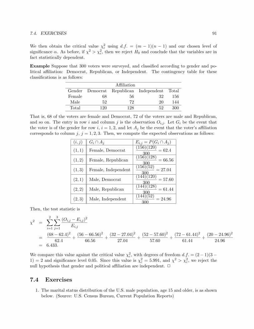
7.4. EXERCISES 91
We then obtain the critical value χ2c using d.f. = (m − 1)(n − 1) and our chosen level of
significance α. As before, if χ2 > χ2c , then we reject H0 and conclude that the variables are in
fact statistically dependent.
Example Suppose that 300 voters were surveyed, and classified according to gender and po-litical affiliation: Democrat, Republican, or Independent. The contingency table for theseclassifications is as follows:
Affiliation
Gender Democrat Republican Independent TotalFemale 68 56 32 156Male 52 72 20 144
Total 120 128 52 300
That is, 68 of the voters are female and Democrat, 72 of the voters are male and Republican,and so on. The entry in row i and column j is the observation Oi,j . Let Gi be the event thatthe voter is of the gender for row i, i = 1, 2, and let Aj be the event that the voter’s affiliationcorresponds to column j, j = 1, 2, 3. Then, we compute the expected observations as follows:
(i, j) Gi ∩Aj Ei,j = P (Gi ∩Aj)
(1, 1) Female, Democrat(156)(120)
300= 62.4
(1, 2) Female, Republican(156)(128)
300= 66.56
(1, 3) Female, Independent(156)(52)
300= 27.04
(2, 1) Male, Democrat(144)(120)
300= 57.60
(2, 2) Male, Republican(144)(128)
300= 61.44
(2, 3) Male, Independent(144)(52)
300= 24.96
Then, the test statistic is
χ2 =
2∑i=1
3∑j=1
(Oi,j − Ei,j)2
Ei,j
=(68− 62.4)2
62.4+
(56− 66.56)2
66.56+
(32− 27.04)2
27.04+
(52− 57.60)2
57.60+
(72− 61.44)2
61.44+
(20− 24.96)2
24.96= 6.433.
We compare this value against the critical value χ2c , with degrees of freedom d.f. = (2− 1)(3−
1) = 2 and significance level 0.05. Since this value is χ2c = 5.991, and χ2 > χ2
c , we reject thenull hypothesis that gender and political affiliation are independent. 2
7.4 Exercises
1. The marital status distribution of the U.S. male population, age 15 and older, is as shownbelow. (Source: U.S. Census Bureau, Current Population Reports)

92 CHAPTER 7. THE CHI-SQUARE DISTRIBUTION
Marital Status Percent Expected Frequency
never married 31.3married 56.1widowed 2.5divorced/separated 10.1
Suppose that a random sample of 400 U.S. young adult males, 18-24 years old, yielded thefollowing frequency distribution. We are interested in whether this age group of males fitsthe distribution of the U.S. adult population. Calculate the frequency one would expectwhen surveying 400 people. Fill in the above table, rounding to two decimal places.
Marital Status Frequency
never married 140married 238widowed 2divorced/separated 20
Does the data fit the expected distribution? Use a significance level of 0.01.
2. College students may be interested in whether or not their majors have any effect onstarting salaries after graduation. Suppose that 300 recent graduates were surveyed as totheir majors in college and their starting salaries after graduation. Below are the data.Conduct a test for independence with a significance level of 0.05.
Major < $50,000 $50,000 - $68,999 $69,000 +
English 5 20 5Engineering 10 30 60Nursing 10 15 15Business 10 20 30Psychology 20 30 20

Chapter 8
Correlation and Simple Regression
In the previous chapter, we learned how to determine whether two random variables werestatistically dependent on one another, using the chi-square goodness-of-fit test. However, thattest alone does not give us any indication of how the variables are related. In this chapter,we will learn how to use correlation and regression to gain some insight into the nature of therelationship between two variables.
8.1 Independent and Dependent Variables
In the following discussion, we classify one of the variables, x, as the independent variable, andthe other variable, y, as the dependent variable. This means that x serves as the “input” andy serves as the “output”. Mathematically, y is a function of x, meaning that y is determinedfrom x in some systematic way. Therefore, for each value of x, there is only one value of y,whereas one value of y can correspond to more than one value of x.
8.2 Correlation
Correlation measures the strength and direction of the relationship between x and y. Types ofcorrelation are:
• positive linear correlation, which means that as x increases, y increases linearly,
• negative linear correlation, which means that as x increases, y decreases linearly,
• nonlinear correlation, which means that there is a clear relationship between x and y, butthe dependence of y on x cannot be described graphically using a straight line, and
• no correlation, which means that there is no clear relationship between x and y.
In the remainder of this discussion, we will limit ourselves to linear correlation.
93

94 CHAPTER 8. CORRELATION AND SIMPLE REGRESSION
8.2.1 Correlation Coefficient
To determine the correlation between two variables x and y, for which we have n observationsof each, we compute the correlation coefficient , which is defined by
r =
nn∑i=1
xiyi −
(n∑i=1
xi
)(n∑i=1
yi
)√√√√√n n∑
i=1
x2i −
(n∑i=1
xi
)2n n∑
i=1
y2i −
(n∑i=1
yi
)2.
Geometrically, r is the cosine of the angle between the vector of x-values and the vector of y-values, with their respective means subtracted. It follows from this interpretation that |r| ≤ 1.If r > 0, then x and y have a positive linear correlation, whereas if r < 0, then x and y havea negative linear correlation. If r = 0, then there is no correlation between x and y. In theextreme cases, r = ±1, we have y = cx for some constant c that is positive (r = 1) or negative(r = −1).
The benefit of knowing whether two variables are linearly correlated is that we can, atleast approximately, predict values of the dependent variable y from values of the independentvariable x. Of course, the accuracy of this prediction depends on |r|; if r is nearly zero, such aprediction is not likely to be reliable.
8.2.2 Testing the Significance of the Correlation Coefficient
Suppose we have determined that x and y are linearly correlated, based on the value of thecorrelation coefficient r obtained from a sample. How do we know whether a similar correlationapplies to the entire population? We can answer this question by performing a hypothesis teston the population correlation coefficient, which we denote by p.
If we only wish to test whether p is nonzero, then we can use a two-tail test, with nullhypothesis H0 : p = 0 and alternative hypothesis H1 : p 6= 0. On the other hand, if we wishto test for a positive linear correlation, we can perform a one-tail test with null hypothesisH0 : p ≤ 0 and alternative hypothesis H1 : p > 0; testing for a negative linear correlation issimilar.
For this test, we use the Student t-distribution. The test statistic is
t∗ =r√
1− r2
n− 2
,
where, as before, n is the sample size for each variable, d.f. = n − 2 is the number of degreesof freedom, and
√(1− r2)/(n− 2) is the standard error of the correlation coefficient. For the
one-tail test with H0 : p ≤ 0, we reject H0 and conclude that x and y have a positive linearcorrelation if t∗ > tα, whereas for the two-tail test with H0 : p = 0, we reject H0 and concludethat x and y are linearly correlated if |t∗| > tα/2.
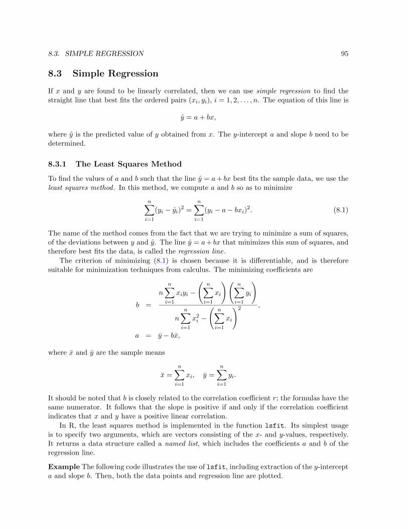
8.3. SIMPLE REGRESSION 95
8.3 Simple Regression
If x and y are found to be linearly correlated, then we can use simple regression to find thestraight line that best fits the ordered pairs (xi, yi), i = 1, 2, . . . , n. The equation of this line is
y = a+ bx,
where y is the predicted value of y obtained from x. The y-intercept a and slope b need to bedetermined.
8.3.1 The Least Squares Method
To find the values of a and b such that the line y = a+ bx best fits the sample data, we use theleast squares method . In this method, we compute a and b so as to minimize
n∑i=1
(yi − yi)2 =n∑i=1
(yi − a− bxi)2. (8.1)
The name of the method comes from the fact that we are trying to minimize a sum of squares,of the deviations between y and y. The line y = a+ bx that minimizes this sum of squares, andtherefore best fits the data, is called the regression line.
The criterion of minimizing (8.1) is chosen because it is differentiable, and is thereforesuitable for minimization techniques from calculus. The minimizing coefficients are
b =
nn∑i=1
xiyi −
(n∑i=1
xi
)(n∑i=1
yi
)
nn∑i=1
x2i −
(n∑i=1
xi
)2 ,
a = y − bx,
where x and y are the sample means
x =
n∑i=1
xi, y =
n∑i=1
yi.
It should be noted that b is closely related to the correlation coefficient r; the formulas have thesame numerator. It follows that the slope is positive if and only if the correlation coefficientindicates that x and y have a positive linear correlation.
In R, the least squares method is implemented in the function lsfit. Its simplest usageis to specify two arguments, which are vectors consisting of the x- and y-values, respectively.It returns a data structure called a named list, which includes the coefficients a and b of theregression line.
Example The following code illustrates the use of lsfit, including extraction of the y-intercepta and slope b. Then, both the data points and regression line are plotted.
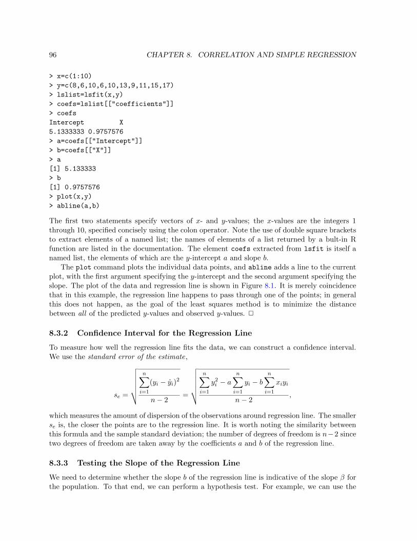
96 CHAPTER 8. CORRELATION AND SIMPLE REGRESSION
> x=c(1:10)
> y=c(8,6,10,6,10,13,9,11,15,17)
> lslist=lsfit(x,y)
> coefs=lslist[["coefficients"]]
> coefs
Intercept X
5.1333333 0.9757576
> a=coefs[["Intercept"]]
> b=coefs[["X"]]
> a
[1] 5.133333
> b
[1] 0.9757576
> plot(x,y)
> abline(a,b)
The first two statements specify vectors of x- and y-values; the x-values are the integers 1through 10, specified concisely using the colon operator. Note the use of double square bracketsto extract elements of a named list; the names of elements of a list returned by a bult-in Rfunction are listed in the documentation. The element coefs extracted from lsfit is itself anamed list, the elements of which are the y-intercept a and slope b.
The plot command plots the individual data points, and abline adds a line to the currentplot, with the first argument specifying the y-intercept and the second argument specifying theslope. The plot of the data and regression line is shown in Figure 8.1. It is merely coincidencethat in this example, the regression line happens to pass through one of the points; in generalthis does not happen, as the goal of the least squares method is to minimize the distancebetween all of the predicted y-values and observed y-values. 2
8.3.2 Confidence Interval for the Regression Line
To measure how well the regression line fits the data, we can construct a confidence interval.We use the standard error of the estimate,
se =
√√√√√√n∑i=1
(yi − yi)2
n− 2=
√√√√√√n∑i=1
y2i − a
n∑i=1
yi − bn∑i=1
xiyi
n− 2,
which measures the amount of dispersion of the observations around regression line. The smallerse is, the closer the points are to the regression line. It is worth noting the similarity betweenthis formula and the sample standard deviation; the number of degrees of freedom is n−2 sincetwo degrees of freedom are taken away by the coefficients a and b of the regression line.
8.3.3 Testing the Slope of the Regression Line
We need to determine whether the slope b of the regression line is indicative of the slope β forthe population. To that end, we can perform a hypothesis test. For example, we can use the

8.3. SIMPLE REGRESSION 97
Figure 8.1: Plot of observations (xi, yi), i = 1, . . . , 10, and corresponding regression line
null hypothesis H0 : β = β0 and H1 : β 6= β0 for a two-tail test. If β0 = 0, then we are testingwhether there is any linear relationship between x and y, and rejection of H0 would imply thatthis is the case.
The standard error of slope is
sb =se√∑n
i=1 x2i − nx2
,
where se is the standard error of the estimate, defined earlier. Note that sb is the standarddeviation in the y-values divided by
√n times the standard deviation of the x-values, which
intuitively makes sense because we are testing the slope, which is the change in y divided bythe change in x.
As with the test of the correlation coefficient, we use the Student’s t-distribution to deter-mine the critical value. The test statistic is
t∗ =b− β0
sb.
This is compared to the critical value tα/2,n−2, the t-value satisfying P (|Tn−2| > tα/2,n−2) = α/2.If |t∗| > tα/2,n−2, then we reject H0 and conclude β 6= β0. If β0 = 0, then our conclusion iswhat x and y are linearly correlated.
It is important to keep in mind that correlation does not imply causation. That is, even ifthere is a strong correlation between x and y, that does not necessarily mean that a change in yis caused by a change in x. It could be mere coincidence, or that some other variable influencesboth x and y in a similar way.

98 CHAPTER 8. CORRELATION AND SIMPLE REGRESSION
8.3.4 The Coefficient of Determination
The strength of the relationship between x and y can be measured by the coefficient of deter-mination, which is defined to be r2, where r is the correlation coefficient. More precisely, thecoefficient of determination measures the percentage of the variation in y that can be explainedby the regression line.
8.3.5 Assumptions
For the least squares method to be valid, we need to make the following assumptions:
• Individual differences between yi and yi, i = 1, 2, . . . , n, are independent of one another.
• The observed values of y are normally distributed around y.
• The variation of y around the regression line is equal for all values of x.
8.4 Nonlinear Regression
8.4.1 Polynomial Regression
In linear regression, we are trying to find constants a and b such that the function y = a+ bxbest fits the data (xi, yi), i = 1, 2, . . . , n, in least-squares sense. The method of least squares canreadily be generalized to the problem of finding constants a0, a2, . . . , am such that the function
y = c0 + c1x+ c2x2 + · · ·+ cmx
m,
a polynomial of degree m, best fits the data. We define the n× (m+ 1) matrix
A =
1 x1 x2
1 · · · xm11 x2 x2
2 · · · xm2...
...1 xn x2
n · · · xmn
,and the vectors
c =
c0
c1...cm
, y =
y1
y2...yn
.A is known as a Vandermonde matrix. Then, by solving the normal equations
ATAc = ATy,
we obtain the coefficients of the best-fitting polynomial of degree m. Note that AT is thetranspose of A, which is obtained by changing rows into columns; that is, (AT )ij = aji.
Example The following R statements construct data vectors x and y, and then call the functionlm (short for “linear model”) to obtain

8.4. NONLINEAR REGRESSION 99
> x=c(0.6291,0.2956,0.6170,0.9885,0.3440,0.2396,0.0004,0.9093,0.6275,0.7862)
> y=c(0.7487,0.6169,0.1834,0.8436,0.7160,0.6518,0.6128,0.8738,0.7927,0.7244)
> lm(y ~ poly(x,2,raw=TRUE))
Call:
lm(formula = y ~ poly(x, 2, raw = TRUE))
Coefficients:
(Intercept) poly(x, 2, raw = TRUE)1 poly(x, 2, raw = TRUE)2
0.6741 -0.4575 0.6512
That is, the quadratic function that best fits the data is y = 0.6512x2 − 0.4575x+ 0.6741. Theexpression y poly(x,2,raw=TRUE) specifies that y is to be treated as a quadratic function ofx. That is, the second argument to poly is the degree. The third argument to poly, raw=TRUE,specifies that the monomial basis 1, x, x2, . . . is to be used, instead of the default behavior ofpoly, which is to use orthogonal polynomials. This is done in order to facilitate interpretationof the coefficients returned by lm. 2
8.4.2 Multiple Linear Regression
A similar approach can be used for multiple linear regression, in which we seek a model of theform
y = c0 + c1x1 + c2x2 + · · ·+ cmxm.
Let xij be the ith observation of xj , for i = 1, 2, . . . , n and j = 1, 2, . . . ,m. We define the matrixA by
A =
1 x11 x12 · · · x1m
1 x21 x22 · · · x2m...
......
1 xn1 xn2 · · · xnm
.Then, we solve the normal equations
ATAc = ATy
to obtain the coefficients c0, c1, . . . , cm.
Example Suppose that we have a set of n observations (xi1, xi2, yi), i = 1, 2, . . . , n, and seekthe coefficients c0, c1, c2 so that the model
y = c0 + c1x1 + c2x2
best fits the data in the least-squares sense. The following R statements obtain these coefficients.
> x1=c(0.4092,0.9977,0.6238,0.3532,0.1827,0.3209,0.2556,0.9411,0.8929,0.9881)
> x2=c(0.9525,0.8742,0.1622,0.1467,0.6498,0.7901,0.0723,0.2445,0.0107,0.2325)
> y=c(0.2549,0.9122,0.3675,0.0380,0.6508,0.8164,0.0838,0.0115,0.3656,0.4128)

100 CHAPTER 8. CORRELATION AND SIMPLE REGRESSION
> lm(y~x1+x2)
Call:
lm(formula = y ~ x1 + x2)
Coefficients:
(Intercept) x1 x2
0.03273 0.18821 0.59569
That is, c0 = 0.03273, c1 = 0.18821, and c2 = 0.59569. 2
8.4.3 Exponential Regression
The least squares method can also be used for models of the form
y = beax,
where a and b are coefficients that are to be determined. Taking the natural logarithm of bothsides yields
ln y = ln b+ ax,
so we can apply the method of least squares to the model
z = c+ ax,
where z = ln y and c = ln b, and then compute b = ec.
8.5 Exercises
1. Describe the pattern in the scatter plot in Figure 8.2, and decide whether the X and Yvariables would be good candidates for linear regression.
A. The X and Y variables have a strong positive linear relationship.
B. The X and Y variables have a strong negative linear relationship.
C. The X and Y variables have a strong nonlinear relationship.
D. The X and Y variables do not have a clear relationship.
2. Describe the pattern in the scatter plot in Figure 8.3, and decide whether the X and Yvariables would be good candidates for linear regression.
A. The X and Y variables have a strong positive linear relationship.
B. The X and Y variables have a strong negative linear relationship.
C. The X and Y variables have a strong nonlinear relationship.
D. The X and Y variables do not have a clear relationship.

8.5. EXERCISES 101
Figure 8.2: Scatter plot for Exercise 1
3. Describe the pattern in the scatter plot in Figure 8.4, and decide whether the X and Yvariables would be good candidates for linear regression.
A. The X and Y variables have a strong positive linear relationship.
B. The X and Y variables have a strong negative linear relationship.
C. The X and Y variables have a strong nonlinear relationship.
D. The X and Y variables do not have a clear relationship.
4. Describe the pattern in the scatter plot in Figure 8.5, and decide whether the X and Yvariables would be good candidates for linear regression.
A. The X and Y variables have a strong positive linear relationship.
B. The X and Y variables have a strong negative linear relationship.
C. The X and Y variables have a strong nonlinear relationship.
D. The X and Y variables do not have a clear relationship.
5. Height (in inches) and weight (in pounds) in a sample of college freshman men have alinear relationship with the following summary statistics:
x = 68.4, y = 141.6, sx = 4.0, sy = 9.6, r = 0.73
Let Y = weight and X = height, and write the regression equation in the form:
y = a+ bx
(a) What is the value of the slope?

102 CHAPTER 8. CORRELATION AND SIMPLE REGRESSION
Figure 8.3: Scatter plot for Exercise 2
(b) What is the value of the y-intercept?
(c) Calculate the predicted weight for someone 68 inches tall.
6. The correlation between body weight and fuel efficiency (measured as miles per gallon)for a sample of 2,012 model cars is −0.56. Calculate the coefficient of determination forthis data.
7. The correlation between high school GPA and freshman college GPA for a sample of 200university students is 0.32. How much variation in freshman college GPA is not explainedby high school GPA?
8. Rounded to two decimal places, what correlation between two variables is necessary tohave a coefficient of determination of at least 0.50?
9. In a sample of 30 cases, two variables have a correlation of 0.33. Do a t-test to see if thisresult is significant at the α = 0.05 level. Use the formula: t = r
√(n− 2)/(1− r2). Are
the variables significantly correlated?
10. In a sample of 25 cases, two variables have a correlation of 0.45. Do a t-test to see if thisresult is significant at the α = 0.05 level. Use the formula: t = r
√(n− 2)/(1− r2). Are
the variables significantly correlated?
11. A study relating the grams of potassium (Y ) to the grams of fiber (X) per serving inenriched flour products (bread, rolls, etc.) produced the equation: y = 25 + 16x
(a) For a product with five grams of fiber per serving, what are the expected grams ofpotassium per serving?

8.5. EXERCISES 103
Figure 8.4: Scatter plot for Exercise 3
(b) Comparing two products, one with three grams of fiber per serving and one with sixgrams of fiber per serving, what is the expected difference in grams of potassium perserving?
12. The following table shows the payroll for 10 NBA teams (in millions) for the 2014-15season, along with the number of wins during the 2013-14 season.
Payroll Wins
88 4473 5771 5470 5170 3669 5969 5069 2868 4066 56
Compute the correlation coefficient. Test whether the correlation coefficient is nonzero atthe 0.05 level.
13. The following table shows the GPA for five graduate students in mathematics, along withtheir quantitative GRE scores. Develop a model that would predict the GPA of a studentbased on their GRE score. What would be the predicted GPA for a student with a GREscore of 150?
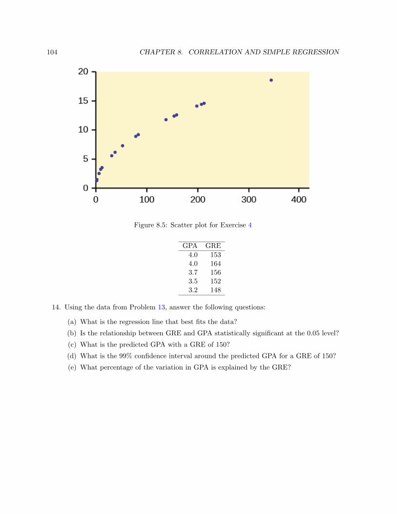
104 CHAPTER 8. CORRELATION AND SIMPLE REGRESSION
Figure 8.5: Scatter plot for Exercise 4
GPA GRE
4.0 1534.0 1643.7 1563.5 1523.2 148
14. Using the data from Problem 13, answer the following questions:
(a) What is the regression line that best fits the data?
(b) Is the relationship between GRE and GPA statistically significant at the 0.05 level?
(c) What is the predicted GPA with a GRE of 150?
(d) What is the 99% confidence interval around the predicted GPA for a GRE of 150?
(e) What percentage of the variation in GPA is explained by the GRE?

Notation
N Population sizen Sample sizeµ Population mean µ = 1
N (x1 + x2 + · · ·+ xN )x Sample mean x = 1
n(x1 + x2 + · · ·+ xn)
µ Weighted mean µ =∑n
i=1 wixi∑ni=1 wi
µ Mean of grouped data µ =∑n
i=1 cifi∑ni=1 fi
ci Class i representative valuefi Frequency of class i
σ2 Population variance 1N
∑Nj=1(xj − µ)2
s2 Sample variance 1n−1
∑nj=1(xj − x)2
Q1 First quartile Median of values less than medianQ2 Median x(n+1)/2 if n odd; 1
2(x(n−1)/2 + xn/2) if n even
Q3 Third quartile Median of values greater than medianIQR Interquartile range Q3 −Q1
S Sample spaceP (A) Probability of event A P (A) = |A|/|S|A′ Complement of A A′ = {x ∈ S|x /∈ A}P (A|B) Conditional probability P (A|B) = P (A ∩B)/P (B)
nPr Permutations nPr = n!/(n− r)!nCr Combinations nCr = n!/[r!(n− r)!]E[X] Expected value E[X] =
∑ni=1 xiP (X = xi)
Var[X] Variance Var[X] = E[X2]− E[X]2
N (µ, σ) Normal distribution mean µ, variance σ2
N (0, 1) Standard normal distributionZ Random variable for N (0, 1)σx Standard error of the mean σx = σ/
√n
p Population proportion p = k/N , k is number of successesps Sample proportion ps = k/n, k is number of successes
σp Standard error of the proportion σp =√p(1− p)/n
105

106 CHAPTER 8. CORRELATION AND SIMPLE REGRESSION
µ0 Null hypothesis test value, meanα Level of significance1− α Confidence levelβ Probability of Type II errorzα Critical z-value P (Z > zα) = αz∗ Test statistic for N (0, 1) z∗ = (x− µ0)/σxE Margin of error E = critical value / standard errorσx Standard error of the mean, σx = s/
√n
variance unknownTn Random variable for Student’s t-distribution d.f. = n degrees of freedomtα,n Critical t-value P (Tn > tα,n) = αt∗ Test statistic for t-distribution t∗ = (x− µ0)/σxp0 Null hypothesis test value, proportion
σx1−x2 Standard error of the difference σx1−x2 =
√σ21n1
+σ22n2
sp Pooled standard deviation sp =
√(n1−1)2s21+(n2−1)2s22
n1+n2−2
σx1−x2 Standard error of the difference, σx1−x2 = sp
√1n1
+ 1n2
unknown equal variances (also σd)
σx1−x2 Standard error of the difference, σx1−x2 =
√s21n1
+s22n2
unknown unequal variances (also σd)sd Sample standard deviation of differences,
dependent samplesσd Standard error of the difference, σd = sd/
√n
dependent samplesp Overall proportion p = (n1p1 + n2p2)/(n1 + n2)
σp1−p2 Standard error of proportion difference, σp1−p2 =
√p(1− p)
(1n1
+ 1n2
)H0 : p1 = p2
σp1−p2 Standard error of proportion difference, σp1−p2 =√
p1(1−p1)n1
+ p2(1−p2)n2
H0 : p1 − p2 = d0
χ2 Chi-square test statistic χ2 =∑
i(Oi − Ei)2/Eiχ2c Critical chi-square value P (χ2 > χ2
c) = αr Correlation coefficient See page 94se Standard error of the estimate See page 96sb Standard error of the slope See page 97

Appendix A
Distribution Tables
A.1 Normal Distribution Table
Table values represent P (Z ≤ z), where z is the z-score.
z .00 .01 .02 .03 .04 .05 .06 .07 .08 .090.0 .50000 .50399 .50798 .51197 .51595 .51994 .52392 .52790 .53188 .535860.1 .53983 .54380 .54776 .55172 .55567 .55962 .56356 .56749 .57142 .575350.2 .57926 .58317 .58706 .59095 .59483 .59871 .60257 .60642 .61026 .614090.3 .61791 .62172 .62552 .62930 .63307 .63683 .64058 .64431 .64803 .651730.4 .65542 .65910 .66276 .66640 .67003 .67364 .67724 .68082 .68439 .687930.5 .69146 .69497 .69847 .70194 .70540 .70884 .71226 .71566 .71904 .722400.6 .72575 .72907 .73237 .73565 .73891 .74215 .74537 .74857 .75175 .754900.7 .75804 .76115 .76424 .76730 .77035 .77337 .77637 .77935 .78230 .785240.8 .78814 .79103 .79389 .79673 .79955 .80234 .80511 .80785 .81057 .813270.9 .81594 .81859 .82121 .82381 .82639 .82894 .83147 .83398 .83646 .838911.0 .84134 .84375 .84614 .84849 .85083 .85314 .85543 .85769 .85993 .862141.1 .86433 .86650 .86864 .87076 .87286 .87493 .87698 .87900 .88100 .882981.2 .88493 .88686 .88877 .89065 .89251 .89435 .89617 .89796 .89973 .901471.3 .90320 .90490 .90658 .90824 .90988 .91149 .91309 .91466 .91621 .917741.4 .91924 .92073 .92220 .92364 .92507 .92647 .92785 .92922 .93056 .931891.5 .93319 .93448 .93574 .93699 .93822 .93943 .94062 .94179 .94295 .944081.6 .94520 .94630 .94738 .94845 .94950 .95053 .95154 .95254 .95352 .954491.7 .95543 .95637 .95728 .95818 .95907 .95994 .96080 .96164 .96246 .963271.8 .96407 .96485 .96562 .96638 .96712 .96784 .96856 .96926 .96995 .970621.9 .97128 .97193 .97257 .97320 .97381 .97441 .97500 .97558 .97615 .976702.0 .97725 .97778 .97831 .97882 .97932 .97982 .98030 .98077 .98124 .981692.1 .98214 .98257 .98300 .98341 .98382 .98422 .98461 .98500 .98537 .985742.2 .98610 .98645 .98679 .98713 .98745 .98778 .98809 .98840 .98870 .988992.3 .98928 .98956 .98983 .99010 .99036 .99061 .99086 .99111 .99134 .991582.4 .99180 .99202 .99224 .99245 .99266 .99286 .99305 .99324 .99343 .993612.5 .99379 .99396 .99413 .99430 .99446 .99461 .99477 .99492 .99506 .995202.6 .99534 .99547 .99560 .99573 .99585 .99598 .99609 .99621 .99632 .996432.7 .99653 .99664 .99674 .99683 .99693 .99702 .99711 .99720 .99728 .997362.8 .99744 .99752 .99760 .99767 .99774 .99781 .99788 .99795 .99801 .998072.9 .99813 .99819 .99825 .99831 .99836 .99841 .99846 .99851 .99856 .99861
107
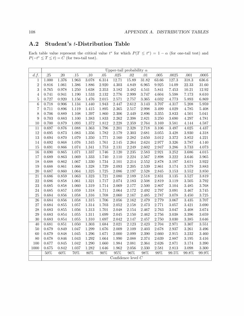
108 APPENDIX A. DISTRIBUTION TABLES
A.2 Student’s t-Distribution Table
Each table value represent the critical value t∗ for which P (T ≤ t∗) = 1 − α (for one-tail test) andP (−t∗ ≤ T ≤ t) = C (for two-tail test).
Upper-tail probability αd.f. .25 .20 .15 .10 .05 .025 .02 .01 .005 .0025 .001 .0005
1 1.000 1.376 1.963 3.078 6.314 12.71 15.89 31.82 63.66 127.3 318.3 636.62 0.816 1.061 1.386 1.886 2.920 4.303 4.849 6.965 9.925 14.09 22.33 31.603 0.765 0.978 1.250 1.638 2.353 3.182 3.482 4.541 5.841 7.453 10.21 12.924 0.741 0.941 1.190 1.533 2.132 2.776 2.999 3.747 4.604 5.598 7.173 8.6105 0.727 0.920 1.156 1.476 2.015 2.571 2.757 3.365 4.032 4.773 5.893 6.8696 0.718 0.906 1.134 1.440 1.943 2.447 2.612 3.143 3.707 4.317 5.208 5.9597 0.711 0.896 1.119 1.415 1.895 2.365 2.517 2.998 3.499 4.029 4.785 5.4088 0.706 0.889 1.108 1.397 1.860 2.306 2.449 2.896 3.355 3.833 4.501 5.0419 0.703 0.883 1.100 1.383 1.833 2.262 2.398 2.821 3.250 3.690 4.297 4.781
10 0.700 0.879 1.093 1.372 1.812 2.228 2.359 2.764 3.169 3.581 4.144 4.58711 0.697 0.876 1.088 1.363 1.796 2.201 2.328 2.718 3.106 3.497 4.025 4.43712 0.695 0.873 1.083 1.356 1.782 2.179 2.303 2.681 3.055 3.428 3.930 4.31813 0.694 0.870 1.079 1.350 1.771 2.160 2.282 2.650 3.012 3.372 3.852 4.22114 0.692 0.868 1.076 1.345 1.761 2.145 2.264 2.624 2.977 3.326 3.787 4.14015 0.691 0.866 1.074 1.341 1.753 2.131 2.249 2.602 2.947 3.286 3.733 4.07316 0.690 0.865 1.071 1.337 1.746 2.120 2.235 2.583 2.921 3.252 3.686 4.01517 0.689 0.863 1.069 1.333 1.740 2.110 2.224 2.567 2.898 3.222 3.646 3.96518 0.688 0.862 1.067 1.330 1.734 2.101 2.214 2.552 2.878 3.197 3.611 3.92219 0.688 0.861 1.066 1.328 1.729 2.093 2.205 2.539 2.861 3.174 3.579 3.88320 0.687 0.860 1.064 1.325 1.725 2.086 2.197 2.528 2.845 3.153 3.552 3.85021 0.686 0.859 1.063 1.323 1.721 2.080 2.189 2.518 2.831 3.135 3.527 3.81922 0.686 0.858 1.061 1.321 1.717 2.074 2.183 2.508 2.819 3.119 3.505 3.79223 0.685 0.858 1.060 1.319 1.714 2.069 2.177 2.500 2.807 3.104 3.485 3.76824 0.685 0.857 1.059 1.318 1.711 2.064 2.172 2.492 2.797 3.091 3.467 3.74525 0.684 0.856 1.058 1.316 1.708 2.060 2.167 2.485 2.787 3.078 3.450 3.72526 0.684 0.856 1.058 1.315 1.706 2.056 2.162 2.479 2.779 3.067 3.435 3.70727 0.684 0.855 1.057 1.314 1.703 2.052 2.158 2.473 2.771 3.057 3.421 3.69028 0.683 0.855 1.056 1.313 1.701 2.048 2.154 2.467 2.763 3.047 3.408 3.67429 0.683 0.854 1.055 1.311 1.699 2.045 2.150 2.462 2.756 3.038 3.396 3.65930 0.683 0.854 1.055 1.310 1.697 2.042 2.147 2.457 2.750 3.030 3.385 3.64640 0.681 0.851 1.050 1.303 1.684 2.021 2.123 2.423 2.704 2.971 3.307 3.55150 0.679 0.849 1.047 1.299 1.676 2.009 2.109 2.403 2.678 2.937 3.261 3.49660 0.679 0.848 1.045 1.296 1.671 2.000 2.099 2.390 2.660 2.915 3.232 3.46080 0.678 0.846 1.043 1.292 1.664 1.990 2.088 2.374 2.639 2.887 3.195 3.416
100 0.677 0.845 1.042 1.290 1.660 1.984 2.081 2.364 2.626 2.871 3.174 3.3901000 0.675 0.842 1.037 1.282 1.646 1.962 2.056 2.330 2.581 2.813 3.098 3.300
50% 60% 70% 80% 90% 95% 96% 98% 99% 99.5% 99.8% 99.9%Confidence level C

A.3. CHI-SQUARE DISTRIBUTION TABLE 109
A.3 Chi-Square Distribution Table
Each table entry represents the value χ2α for which P (χ > χ2
α) = α.
d.f. χ2.995 χ2
.990 χ2.975 χ2
.950 χ2.900 χ2
.100 χ2.050 χ2
.025 χ2.010 χ2
.005
1 0.000 0.000 0.001 0.004 0.016 2.706 3.841 5.024 6.635 7.8792 0.010 0.020 0.051 0.103 0.211 4.605 5.991 7.378 9.210 10.5973 0.072 0.115 0.216 0.352 0.584 6.251 7.815 9.348 11.345 12.8384 0.207 0.297 0.484 0.711 1.064 7.779 9.488 11.143 13.277 14.8605 0.412 0.554 0.831 1.145 1.610 9.236 11.070 12.833 15.086 16.7506 0.676 0.872 1.237 1.635 2.204 10.645 12.592 14.449 16.812 18.5487 0.989 1.239 1.690 2.167 2.833 12.017 14.067 16.013 18.475 20.2788 1.344 1.646 2.180 2.733 3.490 13.362 15.507 17.535 20.090 21.9559 1.735 2.088 2.700 3.325 4.168 14.684 16.919 19.023 21.666 23.58910 2.156 2.558 3.247 3.940 4.865 15.987 18.307 20.483 23.209 25.18811 2.603 3.053 3.816 4.575 5.578 17.275 19.675 21.920 24.725 26.75712 3.074 3.571 4.404 5.226 6.304 18.549 21.026 23.337 26.217 28.30013 3.565 4.107 5.009 5.892 7.042 19.812 22.362 24.736 27.688 29.81914 4.075 4.660 5.629 6.571 7.790 21.064 23.685 26.119 29.141 31.31915 4.601 5.229 6.262 7.261 8.547 22.307 24.996 27.488 30.578 32.80116 5.142 5.812 6.908 7.962 9.312 23.542 26.296 28.845 32.000 34.26717 5.697 6.408 7.564 8.672 10.085 24.769 27.587 30.191 33.409 35.71818 6.265 7.015 8.231 9.390 10.865 25.989 28.869 31.526 34.805 37.15619 6.844 7.633 8.907 10.117 11.651 27.204 30.144 32.852 36.191 38.58220 7.434 8.260 9.591 10.851 12.443 28.412 31.410 34.170 37.566 39.99721 8.034 8.897 10.283 11.591 13.240 29.615 32.671 35.479 38.932 41.40122 8.643 9.542 10.982 12.338 14.041 30.813 33.924 36.781 40.289 42.79623 9.260 10.196 11.689 13.091 14.848 32.007 35.172 38.076 41.638 44.18124 9.886 10.856 12.401 13.848 15.659 33.196 36.415 39.364 42.980 45.55925 10.520 11.524 13.120 14.611 16.473 34.382 37.652 40.646 44.314 46.92826 11.160 12.198 13.844 15.379 17.292 35.563 38.885 41.923 45.642 48.29027 11.808 12.879 14.573 16.151 18.114 36.741 40.113 43.195 46.963 49.64528 12.461 13.565 15.308 16.928 18.939 37.916 41.337 44.461 48.278 50.99329 13.121 14.256 16.047 17.708 19.768 39.087 42.557 45.722 49.588 52.33630 13.787 14.953 16.791 18.493 20.599 40.256 43.773 46.979 50.892 53.67240 20.707 22.164 24.433 26.509 29.051 51.805 55.758 59.342 63.691 66.76650 27.991 29.707 32.357 34.764 37.689 63.167 67.505 71.420 76.154 79.49060 35.534 37.485 40.482 43.188 46.459 74.397 79.082 83.298 88.379 91.95270 43.275 45.442 48.758 51.739 55.329 85.527 90.531 95.023 100.425 104.21580 51.172 53.540 57.153 60.391 64.278 96.578 101.879 106.629 112.329 116.32190 59.196 61.754 65.647 69.126 73.291 107.565 113.145 118.136 124.116 128.299100 67.328 70.065 74.222 77.929 82.358 118.498 124.342 129.561 135.807 140.169

110 APPENDIX A. DISTRIBUTION TABLES
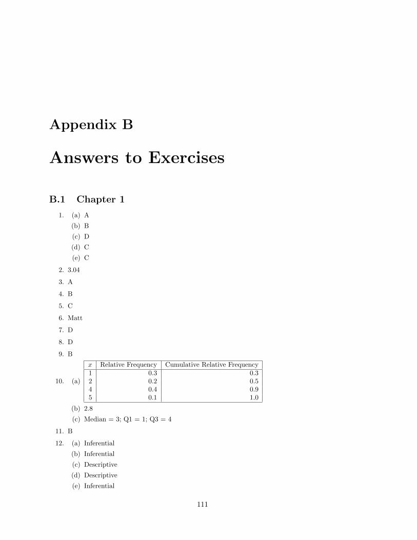
Appendix B
Answers to Exercises
B.1 Chapter 1
1. (a) A
(b) B
(c) D
(d) C
(e) C
2. 3.04
3. A
4. B
5. C
6. Matt
7. D
8. D
9. B
10. (a)
x Relative Frequency Cumulative Relative Frequency1 0.3 0.32 0.2 0.54 0.4 0.95 0.1 1.0
(b) 2.8
(c) Median = 3; Q1 = 1; Q3 = 4
11. B
12. (a) Inferential
(b) Inferential
(c) Descriptive
(d) Descriptive
(e) Inferential
111

112 APPENDIX B. ANSWERS TO EXERCISES
13. (a) Interval
(b) Ratio
(c) Ordinal
(d) Nominal
(e) Ratio
(f) Nominal
(g) Interval
(h) Nominal
(i) Nominal
(j) Ordinal
(k) Nominal
(l) Ordinal
(m) Ratio
14.
Class Frequency20-24 725-29 430-34 335-39 440-44 845-49 10
15.
Histogram of ages
ages
Frequency
20 25 30 35 40 45 50
02
46
810
16.
Class Relative Cumulative20-24 0.1944 725-29 0.1111 1130-34 0.0833 1435-39 0.1111 1840-44 0.2222 2645-49 0.2778 36

B.2. CHAPTER 2 113
17.
[20,25)
[25,30)[30,35)
[35,40)
[40,45)[45,50)
18.2 111334455883 12468994 002233445667788888
19. mean = 11.789, median = 10, mode = 6, variance = 36.674, standard deviation = 6.056, range =22
20. mean = 69.767, standard deviation = 13.451
21. 82.3, 80.6, 74
22. [45, 55]
23. 75%
B.2 Chapter 2
1. (a) 0.24
(b) C
2. B
3. (a) 0.06
(b) 0.44
4. (a) 77/100
(b) 12/42
5. C
6. You will lose $5.
7. (a) 0.02
(b) 0.40
8. (a) Empirical
(b) Classical
(c) Empirical
(d) Classical

114 APPENDIX B. ANSWERS TO EXERCISES
(e) Subjective
(f) Subjective
9. (a) Valid
(b) Invalid
(c) Invalid
(d) Invalid
(e) Valid
(f) Valid
10. (a) P (A)
(b) P (B)
(c) P (A ∩B)
(d) P (A ∪B)
11. (a) P (A) = 167/300
(b) P (B) = 113/300
(c) P (A′) = 133/300
(d) P (B′) = 187/300
(e) P (A|B) = 48/113
(f) P (A′|B) = 65/113
(g) P (A|C) = 94/158
(h) P (A′|C) = 64/158
(i) P (A ∩B) = 48/300
(j) P (A ∩ C) = 94/300
(k) P (A ∪B) = 232/300
(l) P (A ∪ C) = 231/300
(m) P (C|A) = P (A|C)P (C)/P (A) = 94/167
12. 105
13. (1/5)20
14. 720
15. 60C12
16. 32/2, 598960
B.3 Chapter 3
1. (a) 0.0165
(b) 1
2. (a) D
(b) 8
3. P(5)

B.3. CHAPTER 3 115
4. B
5. 0.63
6. D
7. 0.0183
8. (a) C
(b) 0.9951
(c) 12.99
9. C
10. (a) 7.56
(b) 5
(c) 0.943
11. (a) 7.5
(b) 0.0122
12. N (72, 72/√
5)
13. D
14. P (X = 0) = 0.294, P (X = 1) = 0.34, P (X = 3) = 0.244, P (X = 4) = 0.082, P (X = 5) = 0.04.µ = 1.234, σ2 = 1.171, σ = 1.082
15. 10C82−10
16. 5C3(0.75)3(0.25)2
17. 9C7(0.89)7(0.11)2 + 9(0.89)8(0.11) + (0.89)9
18. 20C12(0.2)12(0.8)8
19. (0.97)25 + 25(0.03)(0.97)24 + 25C2(0.03)2(0.97)23
20. P (X = 0) = 0.155, P (X = 1) = 0.35, P (X = 2) = 0.316, P (X = 3) = 0.143, P (X = 4) = 0.0322,P (X = 5) = 0.0029
21. (0.62)5
22. e−121215/15!
23. e−884/4!
24. e−4.55.5
25. 1− e−2.5[3.5 + (2.5)2/2]
26. e−1.51.52/2
27. e−0.75[1.75 + 0.752/2]
28. (a) P (Z > (70− 60)/4) = 0.0062
(b) P (Z ≤ (55− 60)/4) = 0.106
(c) P (|Z| ≤ 2) = 0.95
29. (a) P (Z > 1.25) = 0.106
(b) P (Z ≤ −0.625) = 0.266

116 APPENDIX B. ANSWERS TO EXERCISES
(c) P (|Z| ≤ 2) = 0.68
30. Normal: P (X = 5) = 0.0146. Binomial: P (X = 5) = 20C5(0.5)20 = 0.0148
31. (a) P (Z > 1.2) = 0.115
(b) P (Z ≤ −1.2) = 0.115
32. 0.3872
B.4 Chapter 4
1. stratified sampling
2. (a) C
(b) 0.9990
3. (a) N (2, 0.25/√
32)
(b) 0.5
4. (a) N (7, 0.63)
(b) 0.9911
B.5 Chapter 5
1. (5.52, 8.48)
2. B
3. A
4. (a) Student?s t with df = 15
(b) (560.09, 719.91)
5. (a) (0.0427, 0.0773)
(b) 2,401
6. (a) 0.73
(b) normal
(c) 0.025
(d) 1.4308
(e) (39.57, 42.43)
(f) (39.80, 42.20)
(g) (39.88, 42.12)
7. No

B.6. CHAPTER 6 117
B.6 Chapter 6
1. (a) A
(b) B
(c) −1.19
(d) 0.1172
(e) No
2. B
3. (a) C
(b) 2.21
(c) 0.0135
(d) Reject the null hypothesis.
4. (a) D
(b) t5
5. 0.0006
6. A
7. D
8. H0 : µ = 3.1, H1 : µ 6= 3.1. The population mean is not 3.1 cups per day.
9. The average gasoline consumption in the U.S. is less than 1.8 gallons per car per day. The p-valueis 0.034.
B.7 Chapter 7
1.
Marital Status Percent Expected Frequencynever married 31.3 125.2married 56.1 224.4widowed 2.5 10divorced/separated 10.1 40.4
The data does not fit the distribution.
2. Major and starting salary are not independent.
B.8 Chapter 8
1. A
2. B
3. D
4. C
5. (a) 1.75
(b) 21.76
(c) 140.76
118 APPENDIX B. ANSWERS TO EXERCISES
6. 0.31
7. 0.90
8. 0.71
9. No
10. Yes
11. (a) 105
(b) 48
12. r = −0.074. We do not reject H0, so there is not enough evidence to support the claim that r isnonzero.
13. y = −2.97 + 0.043x; y = 3.483 when x = 150
14. (a) r = 0.752; the relationship is not statistically significant at the 0.05 level.
(b) [1.963, 5.002]
(c) 56.6% of the variation in GPA is explained by the GRE.

Bibliography
[1] de Vries, Andrie and Meys, Joris., R for Dummies. Wiley, 2012.
[2] Dean, Susan and Illowsky, Barbara, Collaborative Statistics, Connexions, 2014.
[3] Donnelly, Robert A., The Complete Idiot’s Guide to Statistics. Penguin Group (USA) Inc., 2007.
[4] Huff, Darrell, How to Lie with Statistics. Norton, 1954.
[5] Ross, Sheldon, Probability and Statistics for Engineers and Scientists, 4th Edition. Academic Press,2009.
119

120 BIBLIOGRAPHY

Index
p-value, 75t-test
paired, 81unpaired, 80
z-score, 48
alternative hypothesis, 71average, see mean
Bayes’ Theorem, 28binomial coefficient, 31binomial distribution, 40box-and-whisker plot, 16
cardinality, 23Central Limit Theorem, 58chart
bar, 10line, 10pie, 9
Chebyshev’s Theorem, 15chi-square goodness-of-fit test, 87chi-square score, 88class, 6cluster, 56coefficient of determination, 98combination, 31complement, 24confidence interval, 56, 63confidence level, 63contingency table, 26correlation, 93
negative, 93nonlinear, 93positive, 93
correlation coefficient, 94
data, 4primary, 4secondary, 4
degrees of freedom, 66
dependent variable, 93descriptive statistics, 1direct observation, 4disjoint sets, 27
empirical rule, 15, 48event, 23
dependent, 27exhaustive, 28independent, 25mutually exclusive, 24, 27
expected value, 38experiment, 4, 23exponential distribution, 46
five-point summary, 16frequency, 6frequency distribution, 6
cumulative, 7relative, 7
Fundamental Counting Principle, 29
histogram, 7hypergeometric distribution, 41hypothesis, 71hypothesis test
one-tail, 73pooled, 81two-tail, 72unpooled, 81
hypothesis testing, 71, 72
independent variable, 93inferential statistics, 1, 2, 63information, 4interquartile range, 15interval estimate, 63
least squares method, 95level of significance, 72linear regression
multiple, 99
121
122 INDEX
margin of error, 64mean, 1, 11, 38
from frequency distribution, 12weighted, 11
measure of central tendency, 10measure of dispersion, 13measurement
interval, 5nominal, 5ordinal, 5ratio, 5
median, 12mode, 13multiplication rule, 26
normal distribution, 46standard, 47
normal equations, 98null hypothesis, 71
outcome, 23
parameter, 4permutation, 30point estimate, 63Poisson process, 42population, 2probability
classical, 23conditional, 25empirical, 24joint, 26posterior, 25prior, 25simple, 25subjective, 24
probability density function, 45, 47probability distribution, 37
discrete, 37probability distribution, continuous, 45probability mass function, 39, 40, 43, 45proportion, 59, 60
quartile, 15first, 15third, 15
random variable, 37continuous, 37, 46discrete, 37
random variable, continuous, 45range, 13regression, 93regression line, 95regression, simple, 95rejection region, 72
sample, 2, 55biased, 2, 55
sample space, 23sampling
cluster, 56random, 55simple, 55stratified, 56systematic, 55with replacment, 30without replacement, 30
sampling distribution, 57for difference of means, 79of the mean, 57
sampling error, 56sigma notation, 11significance level, 64standard deviation, 14
from relative frequency distribution, 15standard error
of the difference, 79of the estimate, 96of the mean, 58of the proportion, 60of the slope, 97
statistic, 4stem-and-leaf display, 8stratus, 56Student’s t-distribution, 66, 77survey, 5
test statistic, 72trial, 39
Bernoulli, 39Type I error, 72Type II error, 72
uniform distribution, continuous, 45uniform distribution, discrete, 39, 57union, 28
variance, 14, 39