Control Tutorials for MATLAB and Simulink - Simulink Basics Tutorial

Prof. Dr. Y. Samim Ünlüsoy ME 513 Vehicle Dynamics 1
Introduction Introduction to Simulinkto Simulink
Prof. Dr. Y. Samim ÜNLÜSOYMech. Eng. Dept., Middle East Technical University, Ankara

Prof. Dr. Y. Samim Ünlüsoy Introduction to Simulink 2
SIMULINKSIMULINKTo start Simulink, one has to first double click on the Matlab icon and wait for the Matlab window to open.
Then, click on the “Simulink” icon

Prof. Dr. Y. Samim Ünlüsoy Introduction to Simulink 3
“Simulink Library Browser”
will open.

Prof. Dr. Y. Samim Ünlüsoy Introduction to Simulink 4
Click on the “File” menu item. Select“New” and then click on “Model”

Prof. Dr. Y. Samim Ünlüsoy Introduction to Simulink 5
A clean window is going to open. New Simulink model is to be built on this window.

Prof. Dr. Y. Samim Ünlüsoy Introduction to Simulink 6
m
kc
z
x
+ + = +mx cx kx cz kz
Consider a one degree of freedom mass-spring-damper system.
Now, let us try to understand the logic behind Simulink, using a familiar system.

Prof. Dr. Y. Samim Ünlüsoy Introduction to Simulink 7
Reorganize the equation of motion such that the highest derivative term
is expressed in terms of the rest :m
kc
z
x
= − − + +c k c kx x x z zm m m m

Prof. Dr. Y. Samim Ünlüsoy Introduction to Simulink 8
SIMULINKSIMULINKNow start with the acceleration and
integrate to get velocity. m
kc
z
x
= − − + +c k c kx x x z zm m m m
Then integrate velocity to get displacement.
xx
xx x
Simulink/Continuous/integrator
1s
1s
1s

Prof. Dr. Y. Samim Ünlüsoy Introduction to Simulink 9
Click on the “integrator”icon inside “continuous”
selection of the “Simulink Library Browser” and drag
it into the model window and leave it there.
Then repeat it for the second integrator.

Prof. Dr. Y. Samim Ünlüsoy Introduction to Simulink 10
Bring the cursor on the arrowhead of the first“integrator” icon and drag it to the arrowtail on the second “integrator” to create the signal line for velocity.

Prof. Dr. Y. Samim Ünlüsoy Introduction to Simulink 11
SIMULINKSIMULINKIt is possible to generate the first two terms on the right hand side.
m
kc
z
x
= − − + +c k c kx x x z zm m m m
xx x
Simulink/Math Operations/
Gain
1s
1s
cm
km
c xm
k xm

Prof. Dr. Y. Samim Ünlüsoy Introduction to Simulink 12
SIMULINKSIMULINK= − − + +c k c kx x x z zm m m m
It is now time to generate the last two terms on the right hand side.
Sine wave
z km
cmdu/dt
z
Simulink/Continuous/
differentiator
Simulink/Sources/
Sine wave xx x1s
1s
cm
km
c zm
k zm

Prof. Dr. Y. Samim Ünlüsoy Introduction to Simulink 13
SIMULINKSIMULINK= − − + +c k c kx x x z zm m m m
Finally sum all the terms and form the acceleration signal.
Sine wave
z km
cmdu/dt
z
xx x1s
1s
cm
km
+--+
Simulink/Math Operations/
sum

Prof. Dr. Y. Samim Ünlüsoy Introduction to Simulink 14
SIMULINKSIMULINK= − − + +c k c kx x x z zm m m m
It is possible to provide different inputs using a switch.
Sine wave
z km
cmdu/dt
z
xx x1s
1s
cm
km
+--+
Constant
A
Manual Switch
Simulink/Sources/constant
Simulink/Signal Routing/Manual Switch

Prof. Dr. Y. Samim Ünlüsoy Introduction to Simulink 15
The resulting Simulink model looks like this !

Prof. Dr. Y. Samim Ünlüsoy Introduction to Simulink 16
You can enter parameter values by clicking on each element.
Sine wave
z km
cmdu/dt
z
xx x1s
1s
cm
km
+--+
Constant
A
Manual Switch
Prof. Dr. Y. Samim Ünlüsoy Introduction to Simulink 17
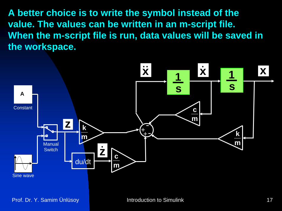
A better choice is to write the symbol instead of the value. The values can be written in an m-script file. When the m-script file is run, data values will be saved in the workspace.
Sine wave
z km
cmdu/dt
z
xx x1s
1s
cm
km
+--+
Constant
A
Manual Switch

Prof. Dr. Y. Samim Ünlüsoy Introduction to Simulink 18
% Data file for sdof.mdlm=310; % [kg]C=980; % [N/m/s]K=15000; % [N/m]A=0.005; % [m]f=2; % [Hz]
Sine wave
z km
cmdu/dt
z
xx x1s
1s
cm
km
+--+
Constant
A
Manual Switch
This is the m-script file to load data to workspace.

Prof. Dr. Y. Samim Ünlüsoy Introduction to Simulink 19
Now, you would like to observe the variation of some variable, say x, with time. So add an oscilloscope !
Sine wave
z km
cmdu/dt
z
xx x1s
1s
cm
km
+--+
Constant
A
Manual Switch
Simulink/Sinks/scope
Scope

Prof. Dr. Y. Samim Ünlüsoy Introduction to Simulink 20
So, the final form of the Simulink diagram is :

Prof. Dr. Y. Samim Ünlüsoy Introduction to Simulink 21
First run the m-file for data by writing its name on the Matlab “Command Window” and pressing enter. Check that the correct data has been stored in workspace.

Prof. Dr. Y. Samim Ünlüsoy Introduction to Simulink 22
Now to run Simulink for 10 seconds, click on the arrow head.

Prof. Dr. Y. Samim Ünlüsoy Introduction to Simulink 23
To see the variation of x with time, double click on the scope.

Prof. Dr. Y. Samim Ünlüsoy Introduction to Simulink 24
The scope window will appear with the plot of x versus time.

Prof. Dr. Y. Samim Ünlüsoy Introduction to Simulink 25
Click on the binoculars icon to fit graph to frame