Introduction to Simio
98
Introduction to Simio Simio LLC 504 Beaver Street Sewickley, Pa 15143 http://www.simio.com Copyright © 2010 Simio LLC. All rights reserved.
description
a tutorial book for simio software
Transcript of Introduction to Simio

Introduction
to Simio
Simio LLC
504 Beaver Street
Sewickley, Pa 15143
http://www.simio.com
Copyright © 2010 Simio LLC. All rights reserved.
Contents
Table of Contents
Chapter 1: Getting Started ............................................................................................................................ 1
Overview ................................................................................................................................................... 1
Models and Projects ................................................................................................................................. 2
The Simio User Interface ........................................................................................................................... 2
Objects and Libraries................................................................................................................................. 4
Instantiating Objects in your Facility Model ............................................................................................. 5
Manipulating Facility Views ...................................................................................................................... 6
Editing Object Properties .......................................................................................................................... 7
A Simple Flow Line Model ......................................................................................................................... 8
Defining Model Properties and Experiments .......................................................................................... 11
Interpreting the Results .......................................................................................................................... 13
Summary ................................................................................................................................................. 15
Chapter 2: Network Travel .......................................................................................................................... 16
Overview ................................................................................................................................................. 16
Entities .................................................................................................................................................... 16
Networks ................................................................................................................................................. 17
Node Routing Logic ................................................................................................................................. 18
Example: Routing by Link Weights .......................................................................................................... 19
Setting the Entity Destination ................................................................................................................. 21
Example: Select From List for Dynamic Routing ..................................................................................... 21
Example: By Sequence ............................................................................................................................ 24
Summary ................................................................................................................................................. 27
Chapter 3: Standard Library ........................................................................................................................ 28
Overview ................................................................................................................................................. 28
Preliminary Concepts .............................................................................................................................. 28
Source and Sink ....................................................................................................................................... 29
Server ...................................................................................................................................................... 33
Combiner and Separator ......................................................................................................................... 35
Example: Combine then Separate ........................................................................................................... 37
Basic Node and Transfer Node ................................................................................................................ 38
Connector, TimePath, and Path .............................................................................................................. 39
Example: Bidirectional Paths................................................................................................................... 39
Conveyors ................................................................................................................................................ 40
Example: Merging Conveyors ................................................................................................................. 41
Vehicle ..................................................................................................................................................... 42
Example: On-Demand Pickups ................................................................................................................ 44
Workstation and Resources .................................................................................................................... 45
Worker .................................................................................................................................................... 47
Example: Moveable Operators ............................................................................................................... 47
Summary ................................................................................................................................................. 49
Chapter 4: Processes ................................................................................................................................... 50
Overview ................................................................................................................................................. 50
Processes ................................................................................................................................................. 50
Process Types .......................................................................................................................................... 52
Building Processes ................................................................................................................................... 53
Steps and Associated Elements .............................................................................................................. 55
Example: Using a Moveable Resource with Server (Seize/Release) ....................................................... 60
Summary ................................................................................................................................................. 62
Chapter 5: Data Driven Models .................................................................................................................. 63
Overview ................................................................................................................................................. 63
Data Tables .............................................................................................................................................. 63
Example: Multiple Entities from a Single Source .................................................................................... 65
Example: Product Routings using Separate Sequence Tables ................................................................ 67
Example: Product Routings using a Table Relation ................................................................................. 70
Example: Initializing an Array using a Table ............................................................................................ 72
Summary ................................................................................................................................................. 76
Chapter 6: Object Definitions ..................................................................................................................... 77
Overview ................................................................................................................................................. 77
Basic Concepts ........................................................................................................................................ 77
External View .......................................................................................................................................... 77
Model Logic ............................................................................................................................................. 79
Properties, States, and Events ................................................................................................................ 81
Example: Tandem Server ........................................................................................................................ 82
Example: A Base Lathe ............................................................................................................................ 84
Example: Server with Repairman ........................................................................................................... 87
Summary ................................................................................................................................................. 90
Glossary ....................................................................................................................................................... 91
Technical Support and Resources ............................................................................................................... 95
Technical Support ................................................................................................................................... 95
Simio User’s Forum ................................................................................................................................. 95
More Information ................................................................................................................................... 95
Using This Material ................................................................................................................................. 95
Introduction to Simio
-1-
Chapter 1: Getting Started
Overview The Simio modeling software lets you build and run dynamic 3D animated models of a wide range of
systems – e.g. factories, supply chains, emergency departments, airports, and service systems. Simio
employs an object approach to modeling, whereby models are built by combining objects that represent
the physical components of the systems.
An object has its own custom behavior as defined by its internal model that responds to events in the
system. For example a production line model is built by placing objects that represent machines,
conveyors, forklift trucks, aisles, etc. You can build your models using the objects provided in the
Standard Object Library, which is general purpose set of objects that comes standard with Simio. You
can also build your own libraries of objects that are customized for specific application areas. As you see
shortly you can also modify and extend the Standard Library object behavior using process logic.
In Simio object definitions and models are the same thing. Whenever you build a model you have
defined the logic for an object that can be used in other models. An object (or model) is defined by its
properties, states, events, external view, and logic. These are key Simio concepts to understand for
building and using objects.
Properties are input values that can be specified by the user of the object. For example an object
representing a server might have a property that specifies the service time. When the user places the
server object into their facility model they would also specify this property value.
An object’s states are dynamic values that may change as the model executes. For example the busy and
idle status of a server object could be maintained by a state variable named Status that is changed by
the object each time it starts or ends service on a customer.
Events are things that the object may “fire” at selected times. For example a server object might have
an event fire each time the server completes processing of a customer, or a tank object might fire an
event whenever it reaches full or empty. Events are useful for informing other objects that something
important has happened.
The external view of an object is the 3D graphical representation of the object. This is what a user of the
object will see when it is placed in their facility model.
The object’s logic is an internal model that defines how the object responds to specific events that may
occur. For example a server object may have a model that specifies what actions take place when a
customer arrives to the server. The internal model gives the object its unique behavior.
One of the powerful features of Simio is that whenever you build a model of a system, you can turn that
model into an object definition by simply adding some input properties and an external view. Your
Introduction to Simio
-2-
model can then be placed as a sub-model within a higher-level model. Hence hierarchical modeling is
very natural in Simio.
Models and Projects When you first open Simio you see a Start Page which includes links to the Simio Reference Guide,
training videos, example models, and SimBits. The SimBits are small models that illustrate how to
approach common modeling situations. From the Start Page you can click on New Model in the ribbon,
or the Create New Model link to open a new model.
Models are defined within a project. A project may contain any number of models and associated
experiments (discussed later). A project will typically contain a main model and an entity model. When
you open up a new project, Simio automatically adds the main model (default name Model) and entity
model (default name ModelEntity) to the project. You can rename the project and these models by
right clicking on them in the project navigation tree. You can also add additional models to the project
by right clicking on the project name. This is typically done to create sub-models that are then used in
building the main model.
The entity model is used to define the behavior of the entities that move through the system. In older
simulation systems entities cannot have behavior, and therefore there is no mechanism for building an
entity model. However in Simio entities can have behaviors that are defined by their own internal
model. The default model entity is “dumb” in that it has no explicit behavior, however as you will see
later you can modify the entity model to take specific actions in response to events. You can also have
multiple types of entity models in your project, with each having its behavior. For example in a model of
an emergency department you could have different entities representing patients, nurses, and doctors.
As we will see later a project can also be loaded into Simio as modeling library. Hence some projects
contain a collection of models for a specific application, and other projects contain models that are
primarily used as building blocks for other models. The same project can either be opened for editing or
be loaded as library.
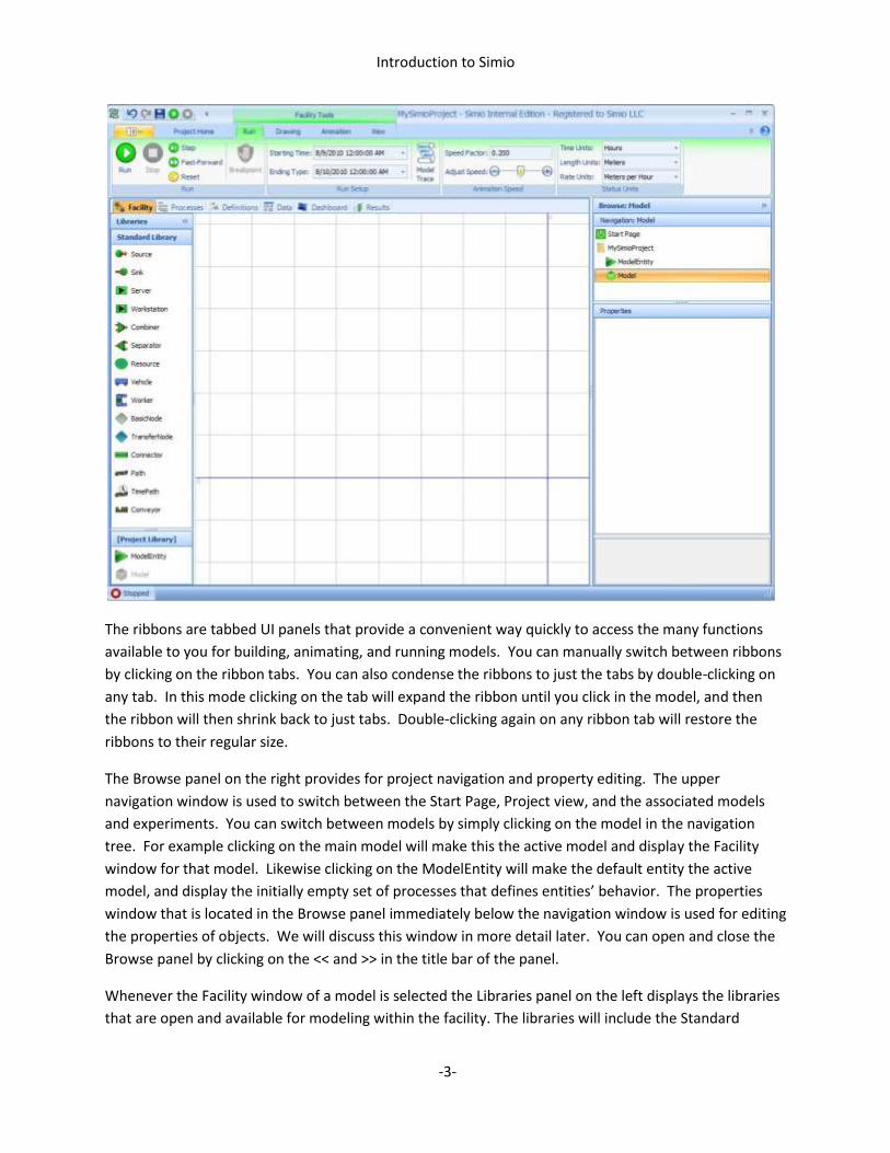
The Simio User Interface The initial view of your Simio project is shown below. The key areas in this screen include the ribbons
across the top (currently showing the Run ribbon), the tabbed panel views with the Facility highlighted
just below the ribbons, the libraries on the left, the browse panel on the right, and the Facility window in
the center.
Introduction to Simio
-3-
The ribbons are tabbed UI panels that provide a convenient way quickly to access the many functions
available to you for building, animating, and running models. You can manually switch between ribbons
by clicking on the ribbon tabs. You can also condense the ribbons to just the tabs by double-clicking on
any tab. In this mode clicking on the tab will expand the ribbon until you click in the model, and then
the ribbon will then shrink back to just tabs. Double-clicking again on any ribbon tab will restore the
ribbons to their regular size.
The Browse panel on the right provides for project navigation and property editing. The upper
navigation window is used to switch between the Start Page, Project view, and the associated models
and experiments. You can switch between models by simply clicking on the model in the navigation
tree. For example clicking on the main model will make this the active model and display the Facility
window for that model. Likewise clicking on the ModelEntity will make the default entity the active
model, and display the initially empty set of processes that defines entities’ behavior. The properties
window that is located in the Browse panel immediately below the navigation window is used for editing
the properties of objects. We will discuss this window in more detail later. You can open and close the
Browse panel by clicking on the << and >> in the title bar of the panel.
Whenever the Facility window of a model is selected the Libraries panel on the left displays the libraries
that are open and available for modeling within the facility. The libraries will include the Standard

Introduction to Simio
-4-
Library, the Project Library, and any additional projects that have been loaded as libraries from the
Project Home ribbon. The Standard Library is a general purpose library of objects that is provided with
Simio for modeling a wide range of systems. The Project Library is a library of objects corresponding to
the current models in your project. This lets you use your project models as sub-models that can be
placed multiple times within a model. Note that the active model is grayed out in the Project Library
since a model cannot be placed inside itself.
The Facility window that is shown in the center is drawing space for building your object-based model.
This panel is shown whenever the Facility tab is selected for a model. This space is used to create both
the object-based logic and the animation for the model in a single step. The other panel views
associated with a model include Process, Definition, Data, Dashboard, and Results. The Process panel is
used for defining custom process logic for your models. The ability to mix object-based and process
modeling within the same model is one of the unique and very powerful features of Simio – this
combines the rapid modeling capabilities of objects with the modeling flexibility of processes. The
Definitions panel is used to define different aspects of the model, such as its external view and the
properties, states, and events that are associated with the model. The Data panel is used to define data
that may be used by the model, and imported/exported to external data sources. The Dashboard panel
provides a 2D drawing space for placing buttons, dials, plots, etc., for real time viewing and interactions
with the model. The Results panel displays the output from the model in the form of both a pivot grid as
well as traditional reports. Note that you can view multiple model windows at the same time by
dragging a window tab and dropping it on one of the layout targets. For now we will be focusing on the
Facility window and will defer further discussion of these additional model windows until later.
Objects and Libraries The objects within a library are one of five basic types:
Fixed: Has a single fixed location in the system such as a machine.
Link: Provides a pathway over which entities may move.
Node: Defines an intersection between one or more incoming/outgoing links. Nodes can also
be associated with fixed objects to provide entry and exit points for the object.
Entity: Defines a dynamic object that can be created and destroyed, move over a network of
links and nodes, and enter/exit fixed objects through their associated nodes.
Transporter: Defines a special type of entity that can also pickup and drop off other entities at
nodes.
Note that these types define the general behavior, but not the specific behavior of the object. The
specific behavior an object is defined by the internal model for that object. For example we could have
a library of a half a dozen different types of transporters, each with their own specific behaviors as
defined by their models. However they would all share the common ability to move across a network of
links and nodes, and pickup and drop off entities at nodes along the way.
A library may contain objects of any these five types. The Standard Library includes objects of all types
except for the entity type, since the entity is typically defined within the Project Library.

Introduction to Simio
-5-
The Standard Library contains the following objects:
Object Description
Source Generates entity objects of a specified type and arrival pattern.
Sink Destroys entities that have completed processing in the model.
Server Represents a capacitated process such as a machine or service operation.
Workstation Models a complex workstation with setup, processing, and teardown phases and secondary resource and material requirements.
Combiner Combines multiple member entities together with a parent entity (e.g. a pallet).
Separator Splits a batched group of entities or makes copies of a single entity.
Resource A generic object that can be seized and released by other objects.
Vehicle A transporter that can follow a fixed route or perform on demand transport pickups/drop offs. Additionally, an ‘On Demand’ routing type vehicle may be used as a moveable resource that is seized and released for non-transport tasks.
Worker A moveable resource that may be seized and released for tasks as well as used to transport entities between node locations.
BasicNode Models a simple intersection between multiple links.
TransferNode Models a complex intersection for changing destination and travel mode.
Connector A simple zero-time travel link between two nodes.
Path A link over which entities may independently move at their own speeds.
TimePath A link that has a specified travel time for all entities.
Conveyor A link that models both accumulating and non-accumulating conveyor devices.
Note that the Standard Library is simply a project in Simio that contains a collection of models that have
been given external views and associated properties that control their behavior.
Instantiating Objects in your Facility Model The object libraries provide definitions for objects that can be placed into the facility model. There are
several different ways to select and place objects into the facility model. For all objects except for links
you can use any of the following methods:
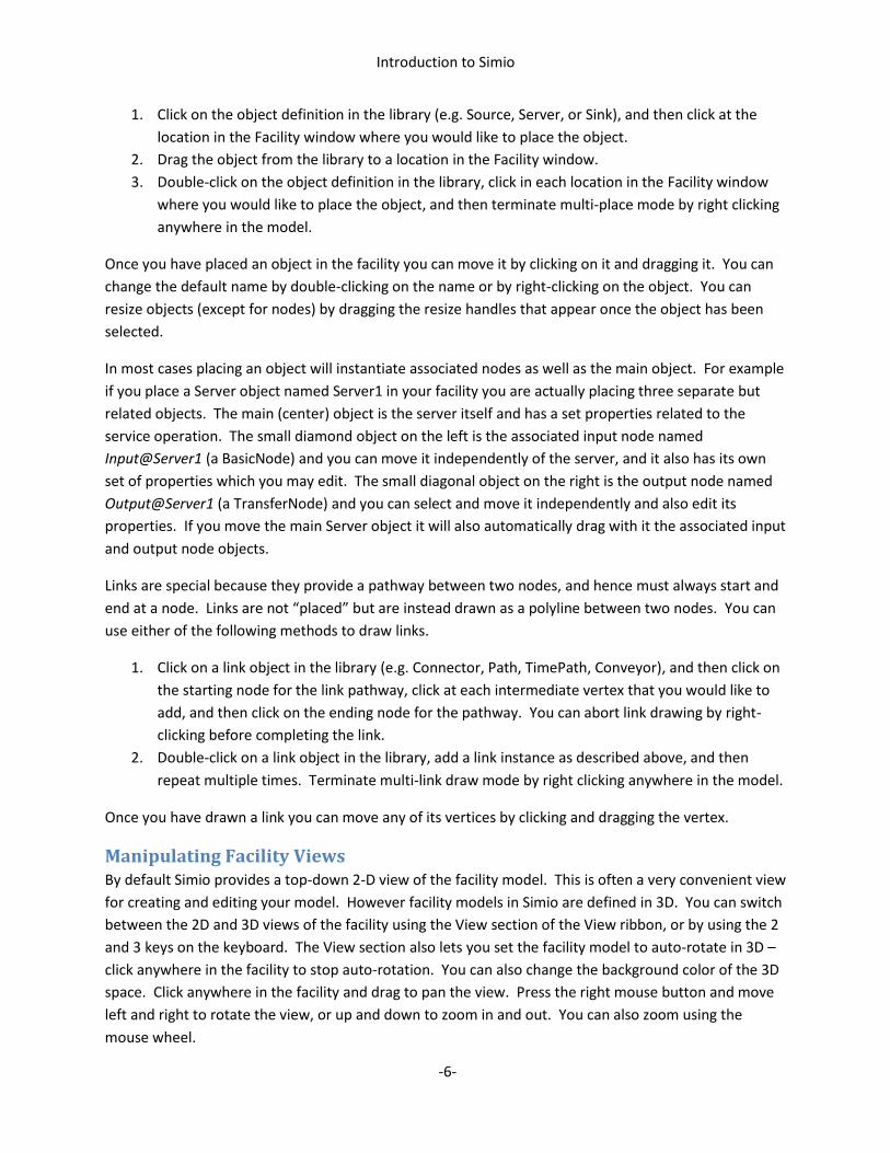
Introduction to Simio
-6-
1. Click on the object definition in the library (e.g. Source, Server, or Sink), and then click at the
location in the Facility window where you would like to place the object.
2. Drag the object from the library to a location in the Facility window.
3. Double-click on the object definition in the library, click in each location in the Facility window
where you would like to place the object, and then terminate multi-place mode by right clicking
anywhere in the model.
Once you have placed an object in the facility you can move it by clicking on it and dragging it. You can
change the default name by double-clicking on the name or by right-clicking on the object. You can
resize objects (except for nodes) by dragging the resize handles that appear once the object has been
selected.
In most cases placing an object will instantiate associated nodes as well as the main object. For example
if you place a Server object named Server1 in your facility you are actually placing three separate but
related objects. The main (center) object is the server itself and has a set properties related to the
service operation. The small diamond object on the left is the associated input node named
Input@Server1 (a BasicNode) and you can move it independently of the server, and it also has its own
set of properties which you may edit. The small diagonal object on the right is the output node named
Output@Server1 (a TransferNode) and you can select and move it independently and also edit its
properties. If you move the main Server object it will also automatically drag with it the associated input
and output node objects.
Links are special because they provide a pathway between two nodes, and hence must always start and
end at a node. Links are not “placed” but are instead drawn as a polyline between two nodes. You can
use either of the following methods to draw links.
1. Click on a link object in the library (e.g. Connector, Path, TimePath, Conveyor), and then click on
the starting node for the link pathway, click at each intermediate vertex that you would like to
add, and then click on the ending node for the pathway. You can abort link drawing by right-
clicking before completing the link.
2. Double-click on a link object in the library, add a link instance as described above, and then
repeat multiple times. Terminate multi-link draw mode by right clicking anywhere in the model.
Once you have drawn a link you can move any of its vertices by clicking and dragging the vertex.
Manipulating Facility Views By default Simio provides a top-down 2-D view of the facility model. This is often a very convenient view
for creating and editing your model. However facility models in Simio are defined in 3D. You can switch
between the 2D and 3D views of the facility using the View section of the View ribbon, or by using the 2
and 3 keys on the keyboard. The View section also lets you set the facility model to auto-rotate in 3D –
click anywhere in the facility to stop auto-rotation. You can also change the background color of the 3D
space. Click anywhere in the facility and drag to pan the view. Press the right mouse button and move
left and right to rotate the view, or up and down to zoom in and out. You can also zoom using the
mouse wheel.

Introduction to Simio
-7-
The visibility section of the View ribbon lets you selectively hide/show different aspects of the facility
model – e.g. you can hide all nodes and links.
You can use the Named Views section of the View ribbon to create and switch to named views into the
facility model – such as the assembly area or shipping. This is a useful feature for navigating through
very large models.
Editing Object Properties Whenever you select an object in the facility (by clicking on it) the properties of the selected object are
displayed for editing in the Property window in the Browse panel on the right. For example, if you select
a Server object in the facility the properties for the Server will be displayed in the Property window. The
properties are organized into categories that can be expanded and collapsed. In the case of the Server
in the Standard Library the Process Logic category is initially expanded, and all others are initially
collapsed. Clicking on +/- will expand and collapse a category. Whenever you select a property in the
property grid a description of the property appears at the bottom of the grid.
The properties for an object are defined by the designer of that object. The properties may be different
types such as strings, numbers, selections from a list, and expressions. For example the Ranking Rule for
the Server is selected from a drop down list and the Processing Time is specified as an expression.
For expression fields (e.g. Processing Time) Simio provides an expression builder to simplify the process
of entering complex expressions. When you click in an expression field a small button with a down
arrow appears on the right. Clicking on this button opens the expression builder. The expression
builder is very similar to IntelliSense® in the Microsoft family of products and tries to find matching
names or keywords as you type. You can use math operators +, – , * , / , and ^ to form expressions.
You can use parenthesis as needed to control the order of calculation (e.g. 2*(3+4)^(4/2) ). Logical
expressions can be expressed using <, <=, >, >=, !=, or ==. Logical expressions return a number value of
1 when true, and 0 when false. For example 10*(A > 2) returns a value of 10 if A is greater than 2.
Arrays (up to 10 dimensions) are 1-based and are indexed with square brackets (e.g. A[2,3,1] indexes
into the three dimensional state array named A). Model properties can be referenced by property
name. For example if Time1 and Time2 are properties that you have added to you model then you can
enter an expression such as (Time1 + Time2)/2.
A common use of the expression builder is to enter random distributions. These are specified in Simio in
the format Random.DistributionName(Parameter1, Parameter2, …, ParameterN), where the number
and meaning of the parameters are distribution dependent. For example Random.Uniform(2,4) will
return a uniform random sample between 2 and 4. To enter this in the expression builder begin typing
“Random”. As you type the highlight in the drop list will jump to the word Random. Typing a period will
then complete the word and display all possible distribution names. Typing a “U” will then jump to
Uniform(min, max). Pressing enter or tab will then add this to the expression. You can then type in the
numeric values to replace the parameter names min and max. Note that highlighting a distribution name
in the list will automatically bring up a description of that distribution.
Introduction to Simio
-8-
Math functions such as Sin, Cos, Log, etc., are accessed in a similar way using the keyword Math. Begin
typing “Math” and enter a period to complete the word and provide a list of all available math functions.
Highlighting a math function in the list will automatically bring up a description of the function.
Object functions may also be referenced by function name. A function is a value that is internally
maintained or computed by Simio and can be used in an expression but cannot be assigned by the user.
For example all objects have function named ID that returns a unique integer for all active objects in the
model. Note that in the case of dynamic entities the ID numbers are reused to avoid generating very
large numbers for an ID.
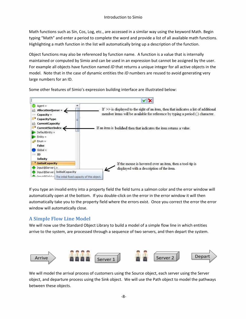
Some other features of Simio’s expression building interface are illustrated below:
If you type an invalid entry into a property field the field turns a salmon color and the error window will
automatically open at the bottom. If you double-click on the error in the error window it will then
automatically take you to the property field where the errors exist. Once you correct the error the error
window will automatically close.
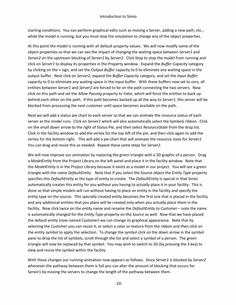
A Simple Flow Line Model We will now use the Standard Object Library to build a model of a simple flow line in which entities
arrive to the system, are processed through a sequence of two servers, and then depart the system.
We will model the arrival process of customers using the Source object, each server using the Server
object, and departure process using the Sink object. We will use the Path object to model the pathways
between these objects.

Introduction to Simio
-9-
The mechanics of building this model is very simple. Open Simio and select New Model. Drag and place
the Source, two Servers, and a Sink. Now double click on the Path object to enter path drawing mode
and connect the output node of the source to the input node of Server 1, connect the output node of
Server 1 to the input node Server 1, and finally connect the output node of Server 2 to the input node of
the Sink. Click anywhere in the drawing space to terminate path drawing mode. Now click on the Run
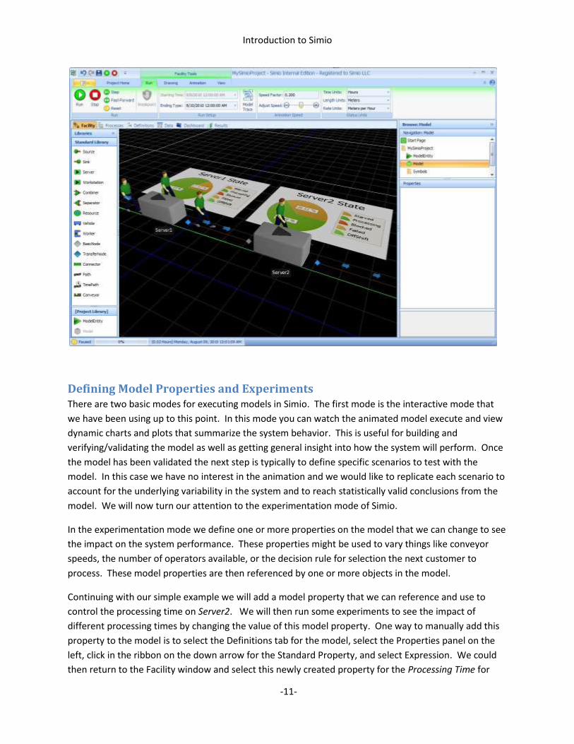
button on the left side of the Run ribbon and you will see your model start executing as shown below.
The green triangles are entities that represent the customers moving through the system. Note that
each server has three green lines representing animations of the queues owned by the server. The
animated queue on the left of the server is the input buffer where customers wait their turn to be
processed, the animated queue above the server is the processing buffer where entities sit while being
serviced, and the animated queue on the right is the output buffer where entities wait to leave the
server. You can move and resize these queue animations. Note that these are animation only constructs
and lengthening the animation queue changes the number of customers that can be animated in the
queue, but not the actual number of customers that can be in the logical queue. The later is changed by
selecting the server and changing the buffer capacities in the Property window. Also note that the
actual number in the queue may exceed the number shown in the animated queue and it may be
necessary to lengthen the animation queue to see all of the entities that are in the queue.
Note that you can pause and restart the simulation, or stop the execution of the model. You can also
step an entity at a time, fast-forward the run without the animation, or reset the model back to its
Introduction to Simio
-10-
starting conditions. You can perform graphical edits such as moving a Server, adding a new path, etc.,
while the model is running, but you must stop the simulation to change any of the object properties.
At this point the model is running with all default property values. We will now modify some of the
object properties so that we can see the impact of changing the waiting space between Server1 and
Server2 on the upstream blocking of Server1 by Server2. Click Stop to stop the model from running and
click on Server1 to display its properties in the Property window. Expand the Buffer Capacity category
by clicking on the + sign, and set the Output Buffer capacity to 0 to eliminate any waiting space in the
output buffer. Next click on Server2, expand the Buffer Capacity category, and set the Input Buffer
capacity to 0 to eliminate any waiting space in the input buffer. With these buffers now set to zero, all
entities between Server1 and Server2 are forced to be on the path connecting the two servers. Now
click on this path and set the Allow Passing property to False, which will force the entities to back up
behind each other on the path. If this path becomes backed up all the way to Server1, this server will be
blocked from processing the next customer until space becomes available on the path.
Next we will add a status pie chart to each server so that we can animate the resource status of each
server as the model runs. Click on Server1 which will also automatically select the Symbols ribbon. Click
on the small down arrow to the right of Status Pie, and then select ResourceState from the drop list.
Click in the facility window to add the vertex for the top left of the pie, and then click again to add the
vertex for the bottom right. This will add a pie chart that will animate the resource state for Server1.
You can drag and resize this as needed. Repeat these same steps for Server2.
We will now improve our animation by replacing the green triangle with a 3D graphic of a person. Drag
a ModelEntity from the Project Library on the left panel and place it in the facility window. Note that
the ModelEntity is in the Project Library because it exists as a model in our project. You will see a green
triangle with the name DefaultEntity. Note that if you select the Source object the Entity Type property
specifies this DefaultEntity as the type of entity to create. The DefaultEntity is special in that Simio
automatically creates this entity for you without you having to actually place it in your facility. This is
done so that simple models will run without having to place an entity in the facility and specify the
entity type on the source. This specially created entity becomes the first one that is placed in the facility
and any additional entities that you place will be created only when you actually place them in the
facility. Now click twice on the entity name and rename the DefaultEntity to Customer – note the name
is automatically changed for the Entity Type property on the Source as well. Now that we have placed
the default entity (now named Customer) we can change its graphical appearance. Note that by
selecting the Customer you can resize it, or select a color or texture from the ribbon and then click on
the entity symbol to apply the selection. To change the symbol click on the down arrow in the symbol
pane to drop the list of symbols, scroll through the list and select a symbol of a person. The green
triangle will now be replaced by that symbol. You may wish to switch to 3D (by pressing the 3 key) to
view and resize the symbol within the facility.
With these changes our running animation now appears as follows. Since Server1 is blocked by Server2
whenever the pathway between them is full you can alter the amount of blocking that occurs for
Server1 by moving the servers to change the length of the pathway between them.
Introduction to Simio
-11-
Defining Model Properties and Experiments There are two basic modes for executing models in Simio. The first mode is the interactive mode that
we have been using up to this point. In this mode you can watch the animated model execute and view
dynamic charts and plots that summarize the system behavior. This is useful for building and
verifying/validating the model as well as getting general insight into how the system will perform. Once
the model has been validated the next step is typically to define specific scenarios to test with the
model. In this case we have no interest in the animation and we would like to replicate each scenario to
account for the underlying variability in the system and to reach statistically valid conclusions from the
model. We will now turn our attention to the experimentation mode of Simio.
In the experimentation mode we define one or more properties on the model that we can change to see
the impact on the system performance. These properties might be used to vary things like conveyor
speeds, the number of operators available, or the decision rule for selection the next customer to
process. These model properties are then referenced by one or more objects in the model.
Continuing with our simple example we will add a model property that we can reference and use to
control the processing time on Server2. We will then run some experiments to see the impact of
different processing times by changing the value of this model property. One way to manually add this
property to the model is to select the Definitions tab for the model, select the Properties panel on the
left, click in the ribbon on the down arrow for the Standard Property, and select Expression. We could
then return to the Facility window and select this newly created property for the Processing Time for
Introduction to Simio
-12-
Server2. However a short cut method to accomplish these same steps is to right click on the Processing
Time property in the Property window for Server2, and select Create New Reference Property. This will
create a new reference property with the default name ProcessingTime, and also specify this as the
value for the Processing Time property. Hence we create the new property and set the reference to it
in a single step.
Now that we have our new referenced property we will define an experiment to see the impact of
varying this property. Add a new experiment by right-clicking on Model in the navigation tree, and
selecting New Experiment. This will create a new experiment with default name Experiment1 and also
select this experiment as the active project component. You can easily return to your model by clicking
on Model in the navigation tree. You can create as many experiments as you like for your model. For
example you might have one experiment to processing times, and another experiment to evaluate
buffer sizes or staffing levels.
Our experiment shows a table, where each row of the table is a scenario to be executed. Note that each
scenario has a check box (enabled/disabled), name, status (initially Idle), and replications required and
completed, and a column for each referenced property on the model. The properties which are
referenced by the model are referred to as Controls since they control the inputs to the model for the
scenario being run. In this example we have a single referenced property named ProcessingTime that is
used to control the processing time for Server2.
We can also add one or more Responses or Constraints to our experiment. A Response can be any valid
expression and is typically a key performance indicator (KPI) that is of particular interest to us in
comparing the scenarios. Although the Pivot Grid and Reports will provide detailed results for the
model, we typically have a few keys parameters that we would like to display directly in the experiment
table. We can also select a specific response to be the Primary Response for the experiment that is
displayed in the Response Chart for the experiment. A Constraint is an expression that must be satisfied
for the scenario to be valid. Both Responses and Constraints may be used by custom add-ins for
defining and evaluating the results from an experiment. For example the OptQuest add-in may be used
to perform an automatic search to optimize the Primary Response, subject to any constraints that have
been defined.
Click on Add Response in the ribbon to add a new response to your experiment. In the property grid
change the response name to TimeInSystem, enter the response expression as
Sink1.TimeInSystem.Average, and select the Objective as Minimize.
We will now define and run three scenarios which we will name Small, Medium, and Large. Enter these
names in the Name column of the table and change the number of required replications to 50. In the
Process Time column change the parameters of the triangular distribution for the Medium scenario to .1,
.23, .33, and in the Large scenario change these values to .1,.26,.36.
Now click on the Run button to initiate the batch running of these scenarios. When you do so you will
see the status for one or more scenarios Running, and the remaining ones listed at Pending. As each
scenario completes its 50 replications it status will change from Running to Completed. If you are

Introduction to Simio
-13-
running on a multi-core processor Simio will automatically assign replications to be executed across
each core of the computer. For example if you have a quad-core processor Simio will run four
replications at a time.
Interpreting the Results Your specific results for this example will depend upon the length for your paths and size of your
customers. However the results should look similar to the following:
Note that in this case the Medium and Large responses for TimeInSystem are grayed out. This is the
result of clicking on the Subset Selection button in the ribbon which causes Simio to automatically
separate the scenarios into two sets for each response: those that might be the best (shown in solid),
and those that can be discarded as not the best (shown grayed-out). This indicates that the Small
scenario can be statistically selected as the single “best” scenario based on minimizing this response. If
the response has more than one member of the “could be best” you can narrow the selection down to a
single scenario using the Select Best Scenario using KN add-in. This add-in employs the sequential
selection method by Kim and Nelson (S. Kim and B. L. Nelson, "A Fully Sequential Procedure for
Indifference-Zone Selection in Simulation," ACM Transactions on Modeling and Computer Simulation 11
(2001), 251-273) to automatically make the required additional runs to narrow the selection down to a
single best scenario.
You can also gain additional insight into your responses by viewing the Response Chart for the primary
response. Click on the Response Chart tab which brings up the following panel and ribbon.
Introduction to Simio
-14-
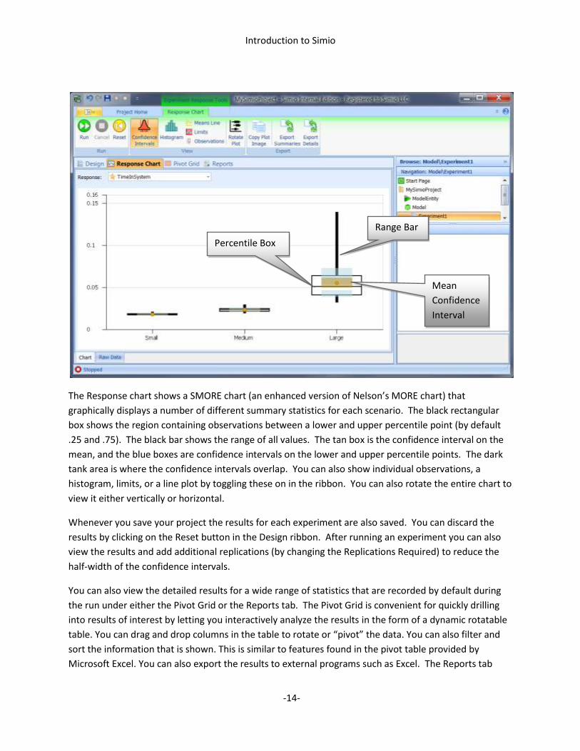
The Response chart shows a SMORE chart (an enhanced version of Nelson’s MORE chart) that
graphically displays a number of different summary statistics for each scenario. The black rectangular
box shows the region containing observations between a lower and upper percentile point (by default
.25 and .75). The black bar shows the range of all values. The tan box is the confidence interval on the
mean, and the blue boxes are confidence intervals on the lower and upper percentile points. The dark
tank area is where the confidence intervals overlap. You can also show individual observations, a
histogram, limits, or a line plot by toggling these on in the ribbon. You can also rotate the entire chart to
view it either vertically or horizontal.
Whenever you save your project the results for each experiment are also saved. You can discard the
results by clicking on the Reset button in the Design ribbon. After running an experiment you can also
view the results and add additional replications (by changing the Replications Required) to reduce the
half-width of the confidence intervals.
You can also view the detailed results for a wide range of statistics that are recorded by default during
the run under either the Pivot Grid or the Reports tab. The Pivot Grid is convenient for quickly drilling
into results of interest by letting you interactively analyze the results in the form of a dynamic rotatable
table. You can drag and drop columns in the table to rotate or “pivot” the data. You can also filter and
sort the information that is shown. This is similar to features found in the pivot table provided by
Microsoft Excel. You can also export the results to external programs such as Excel. The Reports tab
Range Bar
Percentile Box
Mean
Confidence
Interval

Introduction to Simio
-15-
displays a more traditionally formatted report and provides flexible visual formatting for inclusion on
web pages or in printed documents and is useful in presenting results to others.
The results in the Pivot Grid and the Reports show the average, minimum, maximum, and half width for
each of the variables that have been recorded during the simulation. By default the objects in the Simio
Standard Library automatically record a wide range of statistics. As you will see later you can selectively
control the statistics that are recorded.
Summary This paper has introduced the basic modeling concepts of Simio. We have introduced the concept of a
Simio project as a collection of models and associated experiments. We have also introduced the basic
concept of an object and how it is used as a building block for rapidly building and running 3D models in
both an interactive and experimentation mode. In subsequence chapters we will expand on this basic
knowledge to fully explore the modeling power of Simio.
Introduction to Simio
-16-
Chapter 2: Network Travel
Overview In Chapter 1 we introduced the basic concepts for building and running object-based models in Simio. In
our first example we modeled a single line of flow with entities arriving from the Source, proceeding
through the two in-line Servers, and then departing at the Sink. In this chapter we will look at Simio
features for controlling entity and transporter movements. Note that transporters are a special case of
entities: they are entities that can also pick up, carry, and drop off other entities. Hence our description
of entity movements will also apply to transporter movements.
Entities may travel in either free space or over a network of links and nodes. In free space travel an
entity may move without the aid of other objects by setting its direction, speed, and acceleration. In this
case the movement is only governed by the entity and it can freely and independently move through 3D
space. In the case of network travel the entity moves over a constrained set of links and nodes. In this
case the movement is governed by both the entity and the corresponding links and nodes. Note that
different types of links and nodes can produce different types of travel behavior based on the internal
models for those links and nodes. For example one link might impose conveyor-like behavior, and
another link might allow for independent movement and passing. In this chapter we will focus on
network travel.
Entities Entities are dynamic objects that can be created and destroyed, travel over networks, and enter and
depart fixed objects thru their associated node objects. The dynamic entity objects are created from an
entity instance. You typically place one or more entity instances in your model by dragging them in from
your Project library or another custom library. The entity instance has a stationary location and is used
as a “template” for generating dynamic entities that move through the model. Each of the dynamic
entities may have both properties and states. The properties are defined by the entity instance and are
unchangeable during the run and shared across all the dynamic entities. However each dynamic entity
will have its own values for its states which may change as the model runs.
For example, assume we have an entity definition named Person that has properties named Sex and
HairColor, and states named Income and MaritalStatus. Assume that we place two instances of Person;
one we name CustomerTypeA and the other we name CustomerTypeB. We can specify the values for
Sex and HairColor for either CustomerTypeA or CustomerTypeB. All of the dynamic entities that are
generated for CustomerTypeA will all have the same value for these properties, and these values cannot
change during the run. In the same way all of the dynamic entities that are generated for
CustomerTypeB will have the same non-changeable values for Sex and HairColor as defined by the
statically placed entity instance for CustomerTypeB. However each dynamically created Person (from
either CustomerTypeA or CustomerTypeB) will have its own unique value for Income and MaritalStatus
and these values may be changed during the run.
Introduction to Simio
-17-
Networks A network is a collection of one or more links over which entities travel. In Simio you can define as
many networks as you need, and a link can be a member of multiple networks. This latter point is
important for modeling situations where different entities travel on their own networks, but share a
common pathway: e.g. workers and forklift trucks sharing a common aisle. For network travel an entity
must be assigned to a specific network over which they are permitted to travel. The collection of all
links is automatically assigned to a special network called the Global network. By default all entities are
assigned to travel on the Global network (i.e. they can travel on any link). The entity may change its
travel network at any time during the running of the simulation.
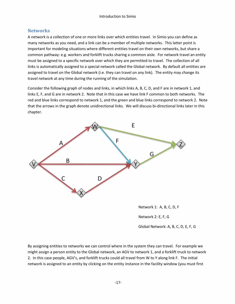
Consider the following graph of nodes and links, in which links A, B, C, D, and F are in network 1, and
links E, F, and G are in network 2. Note that in this case we have link F common to both networks. The
red and blue links correspond to network 1, and the green and blue links correspond to network 2. Note
that the arrows in the graph denote unidirectional links. We will discuss bi-directional links later in this
chapter.
Network 1: A, B, C, D, F
Network 2: E, F, G
Global Network: A, B, C, D, E, F, G
By assigning entities to networks we can control where in the system they can travel. For example we
might assign a person entity to the Global network, an AGV to network 1, and a forklift truck to network
2. In this case people, AGV’s, and forklift trucks could all travel from W to Y along link F. The initial
network is assigned to an entity by clicking on the entity instance in the facility window (you must first
Introduction to Simio
-18-
place the entity instance by dragging it from the Project library) and then setting the Initial Network
property.
In Simio a link may be added to an existing or new network or removed from an existing network by
right clicking on the link. The links that belong to a specific network can be highlighted using the View
Networks drop list on the View ribbon. If multiple networks are selected for highlighting, then either the
Union (links that are a member in one or more of the selected networks) or Intersection (links that are a
member of all selected networks) can be highlighted.
Node Routing Logic Whenever an entity departs a node with more than one departing link in its network then the decision
of which link to travel along is based on the node routing logic. For example an entity traveling on
network 1 and departing node V will have 3 links to choose from based on its routing logic. However an
entity traveling on network 1 and departing node W has only one option: i.e. link F.
In large and complex models we often have alternate pathways through the system and must specify
routing logic for controlling the movement of entities through the system. In the case of the Standard
Library the routing logic for selecting between multiple candidate links is specified by an outbound link
rule and outbound link preference. The outbound link rule specifies how the link is to be selected, and
the outbound link preference specifies if all links are to be considered (Any), or only those that are
currently available (Available). An available link is one that can immediately be entered. The outbound
link rule is specified as either Shortest Path or By Link Weight.
In the case of shortest path the entity will select the path that is along the shortest path to its
destination (note that we will discuss the options for setting the destination for an entity in a moment).
Hence a person traveling on the Global network from V with its destination set to Z would select link B at
node V (assuming B is available or the Any option is selected). If the outbound link rule is specified as
shortest path but the destination is not assigned, then the link is selected by link weights.
When outbound link rule is specified as By Link Weight (or no destination has been set), then the link is
selected randomly using the weights specified for each candidate link. The probability of a given link
being selected is equal to its weight divided by the sum of the weights for the candidate links. All links
have a selection weight property that can be specified as a number or any valid expression. In the
simple case we can use these link weights like percentages or probabilities. For example if one link has a
weight of 80 (or .8) and the other a weight of 20 (or .2), then the links will be selected randomly with an
80/20 split.
In Simio a logical expression (e.g. X > 2) will return a 1 if true, and 0 if false. This makes it very
convenient to use logical expressions for specifying link selection weights. Note that in this case the
weights will dynamically change during the simulation based on the value of the logical expression. For
example, an expression Lathe.InputBuffer.Contents.NumberWaiting == 0 will have a selection value of 1
if the input buffer for the Lathe is empty, otherwise it will have a selection weight of 0.
Introduction to Simio
-19-
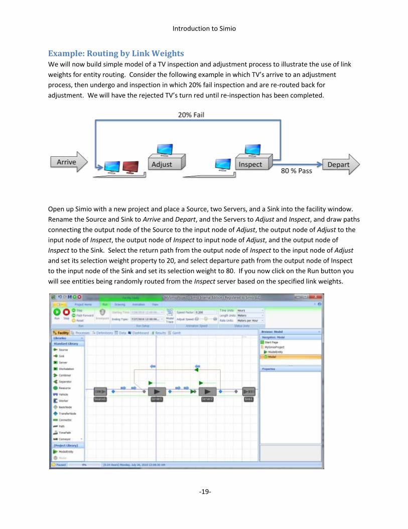
Example: Routing by Link Weights We will now build simple model of a TV inspection and adjustment process to illustrate the use of link
weights for entity routing. Consider the following example in which TV’s arrive to an adjustment
process, then undergo and inspection in which 20% fail inspection and are re-routed back for
adjustment. We will have the rejected TV’s turn red until re-inspection has been completed.
Open up Simio with a new project and place a Source, two Servers, and a Sink into the facility window.
Rename the Source and Sink to Arrive and Depart, and the Servers to Adjust and Inspect, and draw paths
connecting the output node of the Source to the input node of Adjust, the output node of Adjust to the
input node of Inspect, the output node of Inspect to input node of Adjust, and the output node of
Inspect to the Sink. Select the return path from the output node of Inspect to the input node of Adjust
and set its selection weight property to 20, and select departure path from the output node of Inspect
to the input node of the Sink and set its selection weight to 80. If you now click on the Run button you
will see entities being randomly routed from the Inspect server based on the specified link weights.
Introduction to Simio
-20-
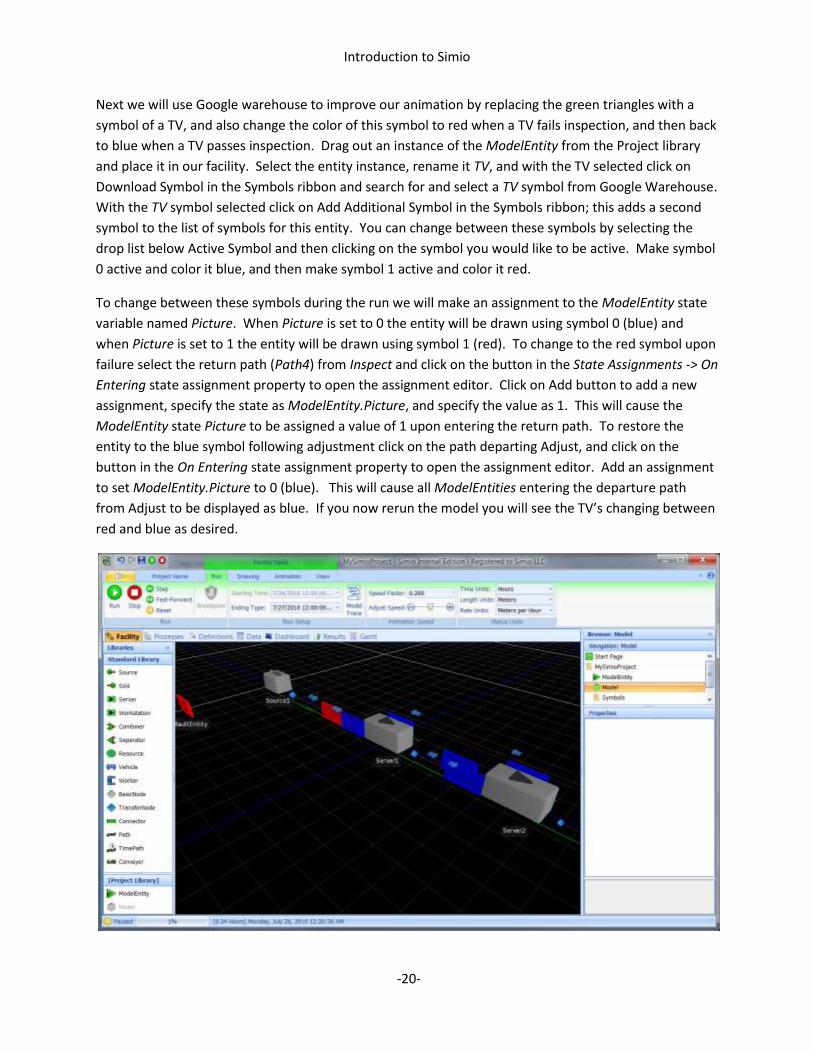
Next we will use Google warehouse to improve our animation by replacing the green triangles with a
symbol of a TV, and also change the color of this symbol to red when a TV fails inspection, and then back
to blue when a TV passes inspection. Drag out an instance of the ModelEntity from the Project library
and place it in our facility. Select the entity instance, rename it TV, and with the TV selected click on
Download Symbol in the Symbols ribbon and search for and select a TV symbol from Google Warehouse.
With the TV symbol selected click on Add Additional Symbol in the Symbols ribbon; this adds a second
symbol to the list of symbols for this entity. You can change between these symbols by selecting the
drop list below Active Symbol and then clicking on the symbol you would like to be active. Make symbol
0 active and color it blue, and then make symbol 1 active and color it red.
To change between these symbols during the run we will make an assignment to the ModelEntity state
variable named Picture. When Picture is set to 0 the entity will be drawn using symbol 0 (blue) and
when Picture is set to 1 the entity will be drawn using symbol 1 (red). To change to the red symbol upon
failure select the return path (Path4) from Inspect and click on the button in the State Assignments -> On
Entering state assignment property to open the assignment editor. Click on Add button to add a new
assignment, specify the state as ModelEntity.Picture, and specify the value as 1. This will cause the
ModelEntity state Picture to be assigned a value of 1 upon entering the return path. To restore the
entity to the blue symbol following adjustment click on the path departing Adjust, and click on the
button in the On Entering state assignment property to open the assignment editor. Add an assignment
to set ModelEntity.Picture to 0 (blue). This will cause all ModelEntities entering the departure path
from Adjust to be displayed as blue. If you now rerun the model you will see the TV’s changing between
red and blue as desired.
Introduction to Simio
-21-
Setting the Entity Destination Whenever the routing logic is based on the shortest path a destination is required for the entity. When
using the Standard Library the destination for an entity may be set using the TransferNode by specifying
the Entity Destination Type and its associated property values. Since the TransferNode is always used
for the output side of the Standard Library fixed objects (Source, Server, Combiner, etc.), you can always
specify the destination for an entity just as it departs any of the fixed objects in the Standard Library. To
specify the destination you click on the TransferNode on the output side of the fixed object and specify
the Entity Destination Type.
There are four options for specifying the Entity Destination Type. The first option is to Continue and
specifies that the entity is to continue without reassigning the destination. This is the default option and
is useful when the entity already has its destination set.
A second option is to specify a Specific destination. In this case a required associated property is
exposed for selecting the Node Name from the drop list. The node maybe be a simple name for a free
standing node (e.g. IntersectionA), or a compound name (e.g. Input@Server1 or Output@Server1) for a
node that is attached as the input or output node of a fixed object. Compound node names are always
specified using the format NodeName@ObjectName.
The third option for specifying a destination is Select From List. In this case we are dynamically selecting
from a list of candidate destinations based on several criteria, which includes a Selection Goal (e.g.
Smallest Distance, Cyclic, etc.), a Selection Condition that must be true for the node to be considered as
a candidate for selection, and a Blocked Routing Rule that specifies if an “unblocked” node is required or
preferred. An unblocked node is one that can immediately accept the entity. For example a Server with
a finite buffer that is full would block any incoming entities.
The fourth option is to specify that the destination is to be set By Sequence. In this case we have
defined a specific visitation sequence (e.g. Drill, Lathe, Inspect, Depart) for each entity and we would like
to set the destination to be the next node in this sequence. This is useful for modeling job shops in
which each entity has a different travel path through the system.
Regardless which method is used to set the destination for the entity, the shortest path routing logic can
then be used to select the link that is on the shortest path to that destination. Note that although the
use of the shortest path rule requires a destination, having a destination does not force you to use the
shortest path rule: i.e. you can still employ link weights to control flow at one more locations along the
way.
The Select From List and By Sequence options are both very useful and powerful methods for setting the
destination for an entity. We will now illustrate each of these more advanced methods with an
example.
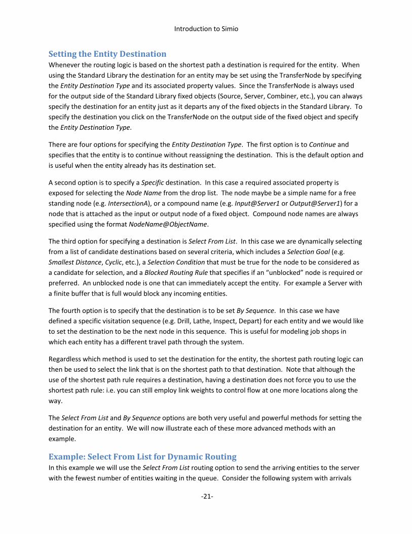
Example: Select From List for Dynamic Routing In this example we will use the Select From List routing option to send the arriving entities to the server
with the fewest number of entities waiting in the queue. Consider the following system with arrivals
Introduction to Simio
-22-
being dynamically directed to one of three servers based on the smallest queue length. Server1 has a
constant processing time of 20 minutes. Server2 has a random processing time in minutes with a
triangular distribution and a minimum of 1, mode of 3, and maximum of 8. Server3 has a processing
time of .1 minutes.
Open up Simio and place a Source, three Servers, and a Sink. Use a Path to connect the Source to the
input node of each of the three servers, and also connect each of the Server output nodes to the Sink.
Edit the Processing Time for each of the servers (select the Processing Time in the Property window and
click on the down arrow to open up the Expression Editor and begin typing) and also set the Input Buffer
capacity for each Server to zero. This will force entities entering the Server to wait on the path since
there is no input buffer available. Change the Allow Passing option on the Paths connecting the output
node for the Source to the input nodes on the Server to False so that the entities will “queue up” along
the path. Note that you can select the first, and then use Control-Click to add the second and third
paths to the selection set, and then simultaneously change this property for all three paths. This same
approach can be used to simultaneously set the input buffer sizes to zero for the three servers.
Before using the Select From List option for selecting the destination we must first define our list of
target nodes. In this case our target nodes are Input@Server1, Input@Server2, and Input@Server3. We
will create a list of these nodes for selecting our destination.
To define a list in Simio click on the Definitions window tab just below the ribbons, and then click on the
Lists icon in the panel selector on the left. In the Create section of the List Data ribbon we can click on
the icons to create a string, object, node, or transporter list. String lists are useful for creating
properties or states that have specific named values (e.g. Small, Medium, Large). Object lists are useful
for selecting specific objects to interact with – e.g. selecting an operator to seize. Transporter lists are
useful for selecting a particular transporter to request a pickup. In this case we click on the node icon to
create a node list of Server input nodes to select from for routing entities. We will give this node list the
name Servers, and populate it with the names of the input nodes for the three servers as follows:

Introduction to Simio
-23-
Now that we have defined our list, we will return to the facility model by clicking on the Facility window
tab. Click on the output node for the Source to specify the routing logic from this node to the three
Servers. In the Routing Logic section of the Property window change the Entity Destination Type to
Select From List, and specify the Node List Name as the newly created node list named Servers. Next set
the Selection Goal to Smallest Value and keep the default Selection Expression as:
Candidate.Node.InputLocation.Overload
Expressions are normally evaluated in the context of the parent object or the entity object executing the
process logic, which in this case is our main model or the entity being routed. When we are searching
the nodes in the list we want to tell Simio to use the context of the candidate object we are looking at in
the search, and not the parent object or routing entity. The keyword Candidate is used for this purpose.
The next part of the expression is telling Simio that the object type being examined is a class Node. The
InputLocation specifies a reference to an input location at this node, typically the input or processing
station at the associated object. Finally the function Overload is a built in function on the Node class
that returns the overload at this node. The overload is defined as the number of entities at this location,
plus the number waiting to enter this location, plus the number of entities traveling with this node as
their destination, minus the capacity at this location. Note that a positive number indicates the input
location is currently overloaded (more there or on the way than the available capacity). A negative
value indicates that capacity is still available based on those at or traveling to the Server.

Introduction to Simio
-24-
Although this will generally balance the load between the three servers, we can make one additional
change to further improve the balance by specifying the Blocked Routing Rule as Prefer Available. Note
that we can have a situation where both Server1 and Server2 are busy, Server3 is idle, but no one is
currently travelling to any of the servers. By specifying the Prefer Available rule we will select Server3 in
this instance, which produces a more balanced flow of work to the three Servers. Our final model with
these options set is shown below:
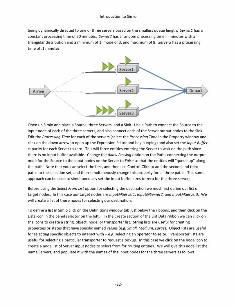
Example: By Sequence In this example we will use the By Sequence option for setting the Entity Destination property. This
option is useful for modeling situations in which an entity follows a specific sequence of destinations
through the model. For example in a job shop each part type might have its own production sequence
through the facility. To illustrate this functionality consider the following example where we have two
different part types being processed across three different servers. Part type A is processed in the
forward direction (Server1, Server2, Server3) and part type B is processed in the reverse direction
(Server3, Server2, Server1).
Introduction to Simio
-25-
In this particular example the two part types do not share common paths. PartA will always travel on a
distinct set of paths (shown in green), and PartB will always travel on a separate set of paths (shown in
red). Hence in this case it would be possible to model this entity flow using two sub-networks. We
would assign the green paths to NetworkA, and the red paths to NetworkB, and have the two part types
follow their own sub-network through the system, creating the desired flow through the system.
However this approach does not work in all cases: e.g. if PartB had a sequence Server3-Server2-Server3.
Routing by sequence provides the flexibility needed to model these more complicated flows.
Begin by opening Simio, creating a new project, and placing the two Sources, three Servers, and Sink.
Also drag out two entity symbols from the Project library and rename them PartA and PartB. Next we
will color PartB red by clicking on the entity symbol, selecting the red color from the Symbols ribbon,
and then clicking on the entity symbol to apply the color. Double click the path symbol in the Standard
Library and draw the forward paths for PartA, and then continue drawing the backward paths for PartB.
Change the Entity Type property for the second Source to PartB. At this point your model should appear
as follows:

Introduction to Simio
-26-
Our next step will be to create sequence tables for PartA and PartB that define their travel sequence
through the system. To do this click on the Data window tab just under the ribbons. The Data window
is used to define various types of data that can be used with your model and we will discuss this
functionality in detail in Chapter 5. For now we will focus on creating Sequence Tables. In the tables
section click on Add Sequence Table and rename the table PartASeq. Repeat this same step and rename
this second table PartBSeq. Next drag the PartBSeq tab and drop it on the right window target so that
we can see both tables simultaneously (you can alternatively right click on either table tab and select
New Vertical Tab Group. Now enter the sequence Input@Server1, Input@Server2, Input@Server3,
Input@Sink1 for PartASeq, and enter Input@Server3, Input@Server2, Input@Server1, Input@Sink for
PartBSeq. At this point your table data should appear as follows:

Introduction to Simio
-27-
If you click on the column labeled Sequence in PartASeq the Property window will display properties for
the sequence. The property Accepts Any Node is by default set to True and allows for any node in the
model to be specified with its fully qualified name (e.g. Input@Server1). You can optionally change this
property to False then only fixed objects may be specified using abbreviated names with the input node
name and @ sign omitted for all fixed objects with a single input node (e.g. a Server). For example the
sequence for ParASeq could be specified as Server1, Server2, Server3, Sink1. This is particularly
convenient when importing routings from external data sources (discussed in Chapter 5).
Now that we have defined our routing sequences we are ready to use them in our model. Click on the
Facility tab to bring the facility window to the front. Click on the PartA entity and set its Initial Sequence
property to PartASeq, and click on the PartB entity and set its Initial Sequence property to PartBSeq.
Now click on the output nodes for the two Sources and three Servers and specify the Entity Destination
Type as By Sequence (you can do this by group selecting with Control-Click). Clicking on the Run button
in the Run ribbon will now start the model executing.
Whenever an entity is routed from a node with the By Sequence option, it automatically bumps its index
into the sequence. Hence each part type will be sent to the next destination that is listed in the
sequence table that it is following. As we will see later you can also change the sequence table that an
entity is following during the simulation (e.g. after failing inspection a part may be assigned to follow a
rework sequence).
Summary This chapter has focused on the concepts related to controlling the flow of entities between objects
across a network of links. These basic concepts can be used to model a wide range of both static and
dynamic entity flows. In the next chapter we will focus on the logic that executes once an entity enters
the objects in the Standard Library.

Introduction to Simio
-28-
Chapter 3: Standard Library
Overview In this chapter we will describe in more detail the objects in the Standard Library. This library is
designed to be a generic modeling library with a broad spectrum of application. So far we have already
made some use of the Source, Server, Sink, and Path objects from this library in the simple models that
we have built so far. We will describe these in more detail, as well as the library objects that we have
yet to use. However before describing these individual objects we will first introduce some general
modeling concepts that are employed by these objects.
Preliminary Concepts As noted in Chapter 1 the objects in Simio have both a general behavior and specific behavior. The
general behavior is defined by one of five basic classes: fixed, node, link, entity, and transporter. A fixed
object models some general activities that take place at a specific location and are triggered by the
arrival an entity. A node object models the starting and/or ending point of one or more links, and also
defines the entry and exit point for a fixed object. Hence most fixed objects have associated node
objects that provide input and output to the object. A link object models the pathway between two
nodes. An entity object can be dynamically created and destroyed, may move through free space or
over a network of links, and move into and out of fixed objects. Finally a transporter is a sub-class of
entity that can also pickup, carry, and drop-off other entities. Although the object class defines the
general behavior of each object, the specific behavior is defined by an internal model for the object
definition. Hence each of these classes can have many different object definitions, each with different
specific behaviors for the corresponding objects that are placed in a model. Hence the Standard Library
is just one of many possible libraries that can be used for modeling. The ability to create custom
libraries is a very powerful feature of Simio.
There are number of important concepts that are employed in designing and building object definitions.
We will explore this topic in more detail in Chapter 6 where we explore the design and building of
custom objects. For now it is important to understand some basic concepts related to stations and
resources.
Many of the objects in the Standard Library make use of the concept of a station. A station is a
construct in Simio that is used to model a constrained location within an object. Entities can transfer
from station to station within an object. Only one entity can transfer into a station at a time, and this
transfer can require time to execute. A station can also have a fixed capacity that will limit the number
of entities that are in process at the station. Whenever a station is at its capacity the station will block
any attempts by other entities to transfer into that station.
As an illustration the Server object employs three stations named InputBuffer, Processing, and
OutputBuffer. An entity first enters the Server at the InputBuffer station, then moves to the Processing
station, and then finally moves to the OutputBuffer station. Each station in Simio has two internal
queues named the EntryQueue and Contents. The queue named EntryQueue holds entities that are
waiting to transfer into the station, and the Contents queue holds the entities that are currently located

Introduction to Simio
-29-
inside the station. Hence the expression Server1.Processing.Contents denotes the queue of entities in
the Processing station at Server1, and the expression Server1.Processing.EntryQueue denotes the queue
of entities waiting to transfer into the Processing station. Likewise the Vehicle object employs a station
named RideStation to hold the entities that are currently riding on the Vehicle.
Many of the objects in the Standard Library also declare themselves as a resource. If an object declares
itself as a resource, then it has a changeable capacity that can be seized and released by other objects.
The object also as a queue named AllocationQueue that holds a prioritized list of other objects that are
waiting to seize it. When capacity becomes available it can be allocated statically based on this
prioritized list, or dynamically based on user-customizable rules. This latter feature makes for very
flexible resource allocation. As we will see later, objects can implement logic to either accept or reject a
seize attempt by another object. When an object is seized a visit request can also be made to have the
seized object travel to a specific location. In this case the request is placed in the VisitRequestQueue for
the object and the object can then decide when and if to visit the requesting object. Hence seizing and
moving a resource object requires cooperation between the seizing object (e.g. a workstation) and the
object being seized/moved (e.g. an operator). These features will be described in more detail in Chapter
5.
Within the Standard Library all of the fixed objects, nodes, and the Vehicle and Worker are declared as
resources. You can also add entities and transporters to your project and declare them as resources.
The Standard Library also contains a fixed object named Resource that is specifically provided for use as
a stationary (non-moving) resource object for seizing and releasing.
All of the objects in the Standard Library support the concept of Add-On processes. An Add-On process
is user-defined process that may be inserted into the object logic at a number of predefined points. As a
result you can actually customize the behavior of these objects without having to create new objects.
We will discuss this functionality in detail in Chapter 4. Most of the Standard Library objects also
support the concept of entity state assignments upon arrival to and/or departure from the object.
Source and Sink As we have already seen in our previous examples, the Source and Sink are fixed objects that are used to
dynamically create and destroy entities. We will now exam each of these objects in more detail.
The Source is comprised of the main Source object plus the associated output node (type TransferNode)
named Output. You independently select and edit both the main Source object and the associated
output node. The main Source object has an OutputBuffer station that holds entities that are waiting to
exit the source through the associated output node. Once an entity successfully transfers into the
network through the output node it then departs the OutputBuffer station that is owned by the Source.
The relationship between the OutputBuffer station that is owned by the Source, and the associated
Output node is shown below:

Introduction to Simio
-30-
By default the Source includes an attached animated queue that displays the entities in its
OutputBuffer.Contents queue. Note that an animated queue can be added as either a detached queue
or an attached Queue. An attached queue is one that is defined in the context of and moves with the
associated object, whereas a detached queue is free-floating and defined in the context of the parent
model. Hence if you drag the Source object the attached animated OutputBuffer.Contents queue will
move with it. If you place a Source, click on the output queue, and press the delete key you will delete
the animated queue. Note that this does not in any way impact the logic for the Source – the logical
station queue still exists – its contents are simply no longer being animated. To re-attach an animation
queue to the Source click on the Source object in the facility, click on the down arrow on the Queue
icon, and select OutputBuffer.Contents from the drop list. To add a detached queue select the
Animation ribbon and click on the Detached Queue icon. In this case you must enter the Queue State
property to animate using the fully qualified name (e.g. Server1.OutputBuffer.Contents).
The arrival logic properties for the main Source object include the Entity Type, Arrival Mode, and Entities
Per Arrival, along with additional properties that switch in and out based on the Arrival Mode. The Entity
Type specifies the type of Entities created by the Source. The Entities Per Arrival property specifies how
many entities are to be created for each arrival event at the source.
The Arrival Mode property governs the pattern of arrivals. The default mode is specified as Interarrival
Time, which switches in properties for specifying the Time Offset for the first arrival, and Interarrival
Time for subsequent arrivals. The mode Time Varying Arrival Rate is used to model a non-homogenous
Poisson arrival process in which the time varies according to a Rate Table that is defined in the Data
window. To create a Rate Table select the Data window, click on Rate Tables in the selection panel on
the left, and then click on Rate Table in the ribbon, which then creates a default Rate Table. A Rate
Table is a set of equal size intervals that specify the mean arrival rate during that interval. Note that the
arrival process is random and so that actual number of arrivals during a given interval may be more or
less than this expected value. You can specify the number of intervals as well as the interval size. The
Rate Table will automatically repeat once it reaches the end of the last interval. The following shows a
Rate Table with six intervals, each four hours long. Once this Rate Table is defined, it can then be
referenced with the Time Varying Arrival Rate mode.

Introduction to Simio
-31-
The mode Arrival Table is used to generate a specific set of arrivals based on arrival times specified in a
table that is defined in the Data window. To use this mode we must first create a table that contains a
list of arrival times that entities enter the system. To create an Arrival Table select the Data window,
click on Tables in the selection panel on the left, and then click on Add Data Table in the ribbon, which
then creates a default Data Table. We will rename this table by changing the Name property in the
Property window to CustomerTable. We will now click on the down arrow for Standard Property and
select a Date Time property to add to the table, and rename this property ArrivalTime. We can enter
arrival time values into this table as shown below:

Introduction to Simio
-32-
Once we have defined are arrival table we can then reference this table and arrival time column using
the Arrival Table mode for the Source object. In this example the Arrival Table is specified as
CustomerTable.ArrivalTime. The Source will then generate arrivals at the times specified in this table.
We will discuss the creation and use of Data Tables in much greater detail in Chapter 5 where we
describe the use of tables for building data driven models.
The On Event mode is used to create a new entity every time an event fires, and switches in a property
for specifying the Event Name for the triggering event. Many of the objects in the Standard Library fire
events at selected times, and we can use these to cause the creation of a new entity. For example
specifying the triggering event as [email protected] would cause the Source to create a new entity
each time an entity entered the input node at Sink1. When selecting this mode you can also specify the
property Initial Number Entities to create an initial set of entities in addition to those that are created
for arrivals that are triggered by each event firing.
Source Stopping Conditions – Note that the Source object also provides a ‘Stopping Conditions’
category of properties that allows you to easily stop arrivals generated by the source using one or more
of the following conditions:
After a specified Maximum Arrivals has occurred.
After a specified Maximum Time has elapsed.

Introduction to Simio
-33-
After a specified event has occurred.
The Sink object is the counterpart to the Source object – it destroys arriving entities and removes them
from the system. The Sink is comprised of the main Sink object plus the associated input node (type
BasicNode) named Input. Only one entity at a time can be processed by the Sink. The Sink has
InputBuffer station that holds the entity being processed for the specified TransferIn Time. Entities are
transferred from the network thru the Input node and into the InputBuffer station. The relationship
between the Input node and InputBuffer station is shown below:
The Sink comes with an attached queue for animating the entity in the InputBuffer station. The Sink
automatically records the average time in system for entities that are destroyed by the Sink.
Server We have used the Server object in several of our previous examples to model a constrained service
operation. The main Server object has two attached objects: an input node (type BasicNode) and an
output node (type TransferNode).
As noted earlier the main Server is modeled with three stations: InputBuffer, Processing, and
OutputBuffer. An arriving entity typically enters from the network through the Input node to the
Server’s InputBuffer, proceeds through Processing, and then waits in the OutputBuffer to move through
the output node and into the network. Note that the network may be blocking an attempt to transfer
out through the Output node (e.g. a path with no passing may be fully backed up and have no available
space). In a similar way when the Server is full it may be blocking the network on the input side.
Both the InputBuffer and the OutputBuffer stations can have their capacities set to zero which causes
them to be removed from the logic. Hence if the OutputBuffer capacity is specified as zero the entity

Introduction to Simio
-34-
completing Processing will wait in Processing to move through the output node and into the network.
Likewise if the InputBuffer capacity is set to zero, then entities that are entering from the network
through the input node must proceed directly to the Processing station of the Server. If the Processing
station is at its capacity it will block entities attempting to enter the Server.
Whenever processing capacity becomes available the next entity to be processed is selected from the
InputBuffer. The InputBuffer is ranked based on the Ranking Rule property, that can be specified as First
In First Out, Last In First Out, Smallest Value First, or Largest Value First. In the last two cases you specify
an expression on which the ranking is based – e.g. you could rank the queue based on processing time
or due date. If no Dynamic Selection Rule is specified then the first entity in the statically ranked queue
is selected for processing. However if a Dynamic Selection Rule is specified, then all entities in the queue
are examined and considered for selection based on the specified rule. These rules include Smallest
Value First and Largest Value First, which from their name seem like similar options to the simple
Ranking Rule. However this dynamic rule is actually more flexible and powerful (although slower to
execute) because it re-evaluates the expression for each entity at the time each decision is made. For
example an expression that has a term that computes if the entity is tardy (by comparing its due date to
the current time) would correctly use the current time when making this decision, and not the arrival
time to the queue. The three campaign rules are used to make selections in an increasing or decreasing
order based on a specified expression. For example, a Server modeling a painting operation may move
from light to dark colors, and then start over with the lightest color once no darker colors remain.
The TransferIn Time property on the Server specifies the time required for an entity to transfer into the
Server object. Only one entity may transfer at a time, and processing of the entity may not start until
this transfer is completed. The Processing Time property specifies the time required to process the
entity at the Processing station.
The Server object can be used to model either a single server or a single processing center with multiple
identical servers, depending upon the capacity specified for the Processing station. The Processing
station is governed by a Capacity Type that is specified as either a Fixed capacity, or based on a
WorkSchedule. To specify a capacity based on a WorkSchedule first create a schedule by clicking on the
Data window, selecting the Schedules panel on the left, and then clicking on Add Schedule in the
Schedule ribbon. A schedule is made up of two parts: a repeating work cycle with superimposed work
exceptions. A work cycle defines a repeating work pattern that defaults to seven days, but can be set to
any arbitrary number of days. You then define the cycle items that define on and off shift periods within
the repeating work cycle. By default the schedule is off shift, so normally you only define the on shift
periods. You can either add cycle items to the work cycle from the ribbon, or you can right click at any
location on the work schedule to add a new item. You can drag any cycle item to a new location, stretch
its length. You can copy a cycle item by clicking the day where you are copying to, then hold down the
CTRL key and select the item that is to be copied, and drag it to the day where it should be copied. You
add and edit work exceptions in a similar way. A work exception is use to override the underlying work
schedule – e.g. to specify holidays or overtime. The following shows a simple seven-day work schedule
named StandardShift that defines a capacity of one from 8-12 and 1-5 on Monday thru Friday. Note that
a single work schedule can be referenced by multiple servers.

Introduction to Simio
-35-
When modeling multiple servers there is always the option to model each server as a separate Server
object in Simio, or use a single Server object with a capacity set to the number of servers. The latter is
far simpler and will produce identical results as long as all the servers have the same performance
characteristics, and waiting customers always go to an available server.
The Server also provides options for failures that halt processing by the Server during the failure. The
failures supported include Calendar Time Based, Processing Count Based, and Event Count Based. In all
three cases the failure duration is specified by the Time To Repair property.
By default the Server object has animated queues for the InputBuffer, Processing, and OutputBuffer.
Again these are animation only constructs and have no impact on the logic of the Server. It may be
necessary to lengthen the animation queue to see all the entities that are actually in the station.
Combiner and Separator The Combiner and Separator are similar to the Server in many ways, however provide additional
functionality to combine several entities together, and then to separate them or to make copies of a
single entity.
The Combiner is used to model a process that matches multiple entities, groups those entities into a
batch, and then attaches those batched members to a parent entity. For example, if we have parts
being placed on a palette, the batched members would be the parts, and the parent entity would be the
palette. The individual batched entities can later be split out using the Separate.

Introduction to Simio
-36-
The Combiner is comprised of a main object plus three associated node objects, including an input node
named ParentInput for the parent entities, an input node named MemberInput for the member entities,
and an output node named Output for the batched entities. The main Combiner object has four
stations: ParentInputBuffer, MemberInputBuffer, Processing, and OutputBuffer. Arriving parent entities
transfer from the network thru the ParentInput node to the ParentInputBuffer station, and arriving
member entities transfer from the network thru the MemberInput node to the MemberInputBuffer
station. The entities are then formed into batches in the Processing station, and then wait in the
OutputBuffer station to depart into the network through the Output node. The relationship between
these node objects and the associated stations is shown below:
The properties for the Combiner include the Batch Quantity and Matching Rule. A batch is formed by
selecting the number of members specified by the Batch Quantity from the member queue, and
attaching them as a batch to a single parent entity selected from the parent queue. The Matching Rule
options include Any Entity, Match Members, and Match Members and Parent. In the case of Any Entity
then entities are selected in the order that they are ranked in the queue. In the case of Match Members
then a batch can only be formed if the member entities all have the same value for the Member Match
Expression. In the case of Match Members and Parent then a batch can only be formed if the member
entities all have the same value for the Member Match Expression, and there is a waiting parent entity
with the same value for the Parent Match Expression. The batched members are carried by the parent
entity in a queue named BatchMembers which can be animated on the parent entity symbol.
The processing capacity and reliability for the Combiner are specified similar to the Server. A good way
to think about the Combiner is that it’s a special purpose Server with two input nodes and special
processing logic for batching.
The Separator is used to model a process that separates batched members from a parent entity, or
makes copies of an entity. Essentially the Separator is a mirror image of the Combiner. The Separator is
comprised of a main object plus three associated node objects, including an input node named Input for
the arriving parent entities, an output node named ParentOutput for the departing parent entities, and
an output node named MemberOutput for the departing member entities. The main Separator object
has four stations: InputBuffer, Processing, ParentOutputBuffer, and MemberOutputBuffer. Arriving
parent entities transfer from the network thru the Input node to the InputBuffer station. The entities
are then split apart or copied in the Processing station, and then the parent entities wait in the
ParentOutputBuffer station to depart into the network through the ParentOutput node, and the

Introduction to Simio
-37-
member entities wait in the MemberOutputBuffer station to depart to the network thru the
MemberOutput node. The relationship between these node objects and the associated stations is shown
below:
The processing logic for the Separator is controlled by the Separation Mode that can be specified as
either Split Batch or Make Copies. In the case of the Split Batch option, entities that are carried by the
parent entity in its BatchMembers queue are split off and transferred to the MemberOutputBuffer
where they wait to depart the Separator. The parent entity is then transferred to the
ParentOutputBuffer when it waits to depart the Separator. The number of entities that are split off is
specified by the Split Quantity property which defaults to the total number of members in the parent
entity’s BatchMembers queue. In the case of the Make Copies option members are created by cloning
the parent entity, with the number of newly created members specified by the Copy Quantity.
Example: Combine then Separate In this example we will model the arrival of two different entity types that have independent arrival
processes and are combined together, processed as a combined batch, and then un-batched before
departing the systems. Each entity type arrives randomly with an exponential time between arrivals
with a mean of 1 minute. The time to batch two entities is a constant .5 minutes, and the time required
to un-batch the entities is a constant 1 minute. The processing time for the combined batch has a
triangular distribution with a minimum of .5, mode of .8, and maximum of 1.2 minutes.
Begin by opening Simio and selecting a new model Project. Now place two entities from the Project
Library and rename them Parent and Member. Resize the Parent entity to make it larger. Select the
Parent entity and click on the down arrow below the Queue icon on the Symbols ribbon and select
BatchMembers. Using the cross hair cursor draw the attached queue just above the Parent entity (make
sure it’s long enough to contain at least one Member entity) and then terminate queue drawing with a
right-click. Note that this attached queue will animate any member entities that are held in the
BatchMembers of the Parent entity. Now select the Member entity, select the color red, and click on
the Member entity again to apply the color. Drag out two Sources, a Combiner, a Server, a Separator,
and two Sinks from the Standard Library. Now connect the objects with Paths as shown below:
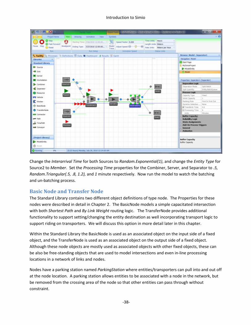
Introduction to Simio
-38-
Change the Interarrival Time for both Sources to Random.Exponential(1), and change the Entity Type for
Source2 to Member. Set the Processing Time properties for the Combiner, Server, and Separator to .5,
Random.Triangular(.5, .8, 1.2), and 1 minute respectively. Now run the model to watch the batching
and un-batching process.
Basic Node and Transfer Node The Standard Library contains two different object definitions of type node. The Properties for these
nodes were described in detail in Chapter 2. The BasicNode models a simple capacitated intersection
with both Shortest Path and By Link Weight routing logic. The TransferNode provides additional
functionality to support setting/changing the entity destination as well incorporating transport logic to
support riding on transporters. We will discuss this option in more detail later in this chapter.
Within the Standard Library the BasicNode is used as an associated object on the input side of a fixed
object, and the TransferNode is used as an associated object on the output side of a fixed object.
Although these node objects are mostly used as associated objects with other fixed objects, these can
be also be free-standing objects that are used to model intersections and even in-line processing
locations in a network of links and nodes.
Nodes have a parking station named ParkingStation where entities/transporters can pull into and out off
at the node location. A parking station allows entities to be associated with a node in the network, but
be removed from the crossing area of the node so that other entities can pass through without
constraint.
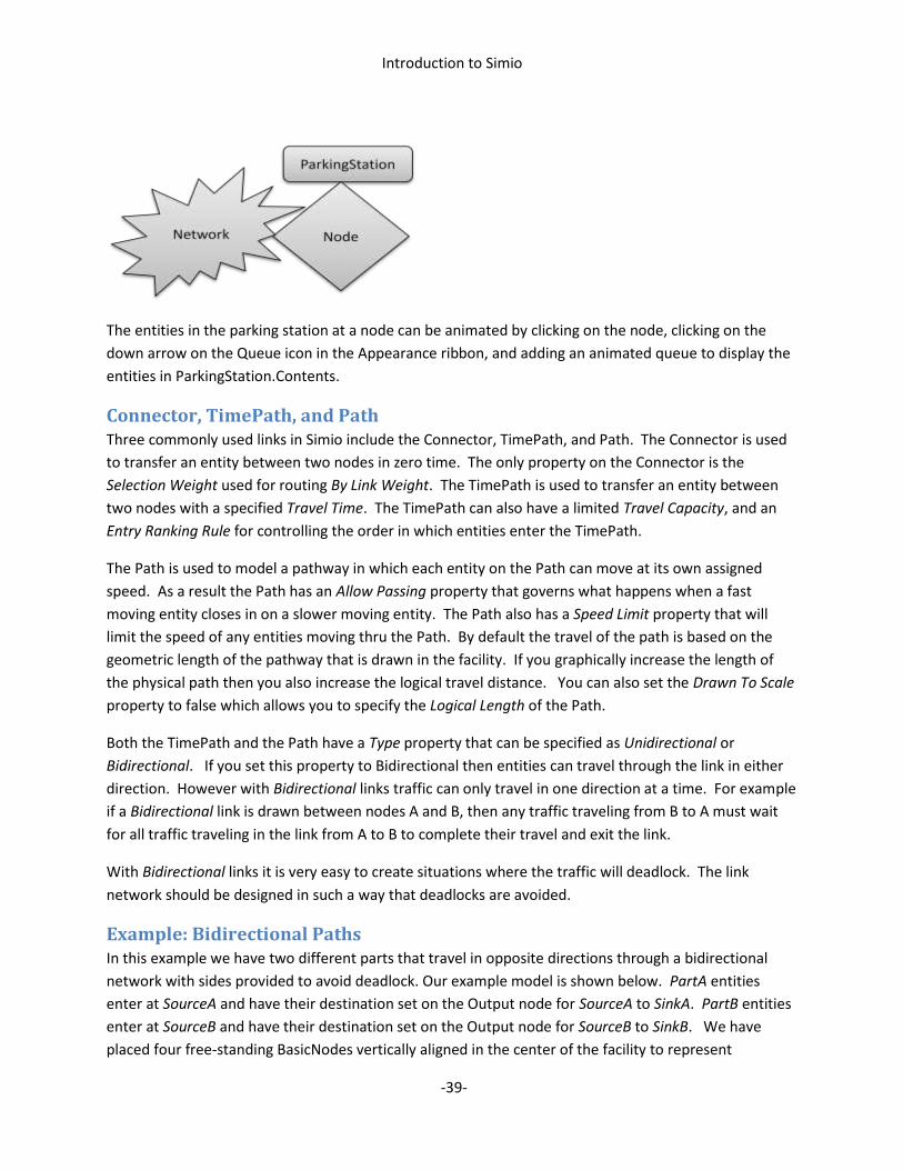
Introduction to Simio
-39-
The entities in the parking station at a node can be animated by clicking on the node, clicking on the
down arrow on the Queue icon in the Appearance ribbon, and adding an animated queue to display the
entities in ParkingStation.Contents.
Connector, TimePath, and Path Three commonly used links in Simio include the Connector, TimePath, and Path. The Connector is used
to transfer an entity between two nodes in zero time. The only property on the Connector is the
Selection Weight used for routing By Link Weight. The TimePath is used to transfer an entity between
two nodes with a specified Travel Time. The TimePath can also have a limited Travel Capacity, and an
Entry Ranking Rule for controlling the order in which entities enter the TimePath.
The Path is used to model a pathway in which each entity on the Path can move at its own assigned
speed. As a result the Path has an Allow Passing property that governs what happens when a fast
moving entity closes in on a slower moving entity. The Path also has a Speed Limit property that will
limit the speed of any entities moving thru the Path. By default the travel of the path is based on the
geometric length of the pathway that is drawn in the facility. If you graphically increase the length of
the physical path then you also increase the logical travel distance. You can also set the Drawn To Scale
property to false which allows you to specify the Logical Length of the Path.
Both the TimePath and the Path have a Type property that can be specified as Unidirectional or
Bidirectional. If you set this property to Bidirectional then entities can travel through the link in either
direction. However with Bidirectional links traffic can only travel in one direction at a time. For example
if a Bidirectional link is drawn between nodes A and B, then any traffic traveling from B to A must wait
for all traffic traveling in the link from A to B to complete their travel and exit the link.
With Bidirectional links it is very easy to create situations where the traffic will deadlock. The link
network should be designed in such a way that deadlocks are avoided.
Example: Bidirectional Paths In this example we have two different parts that travel in opposite directions through a bidirectional
network with sides provided to avoid deadlock. Our example model is shown below. PartA entities
enter at SourceA and have their destination set on the Output node for SourceA to SinkA. PartB entities
enter at SourceB and have their destination set on the Output node for SourceB to SinkB. We have
placed four free-standing BasicNodes vertically aligned in the center of the facility to represent
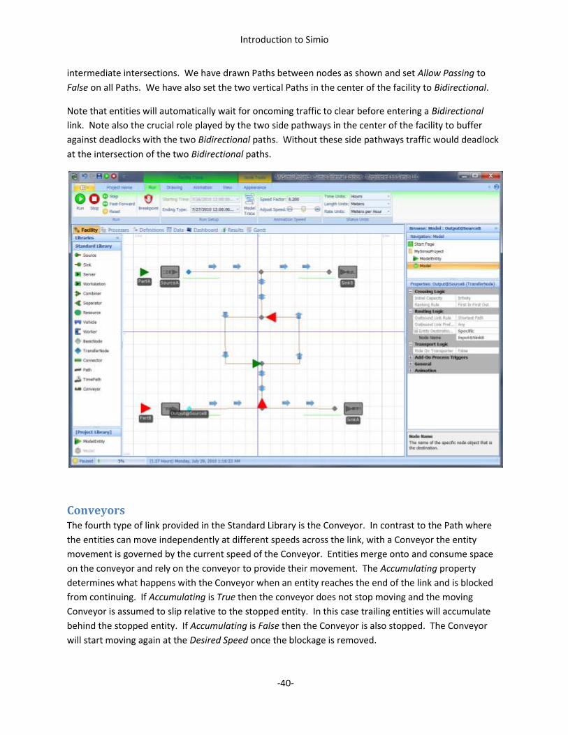
Introduction to Simio
-40-
intermediate intersections. We have drawn Paths between nodes as shown and set Allow Passing to
False on all Paths. We have also set the two vertical Paths in the center of the facility to Bidirectional.
Note that entities will automatically wait for oncoming traffic to clear before entering a Bidirectional
link. Note also the crucial role played by the two side pathways in the center of the facility to buffer
against deadlocks with the two Bidirectional paths. Without these side pathways traffic would deadlock
at the intersection of the two Bidirectional paths.
Conveyors The fourth type of link provided in the Standard Library is the Conveyor. In contrast to the Path where
the entities can move independently at different speeds across the link, with a Conveyor the entity
movement is governed by the current speed of the Conveyor. Entities merge onto and consume space
on the conveyor and rely on the conveyor to provide their movement. The Accumulating property
determines what happens with the Conveyor when an entity reaches the end of the link and is blocked
from continuing. If Accumulating is True then the conveyor does not stop moving and the moving
Conveyor is assumed to slip relative to the stopped entity. In this case trailing entities will accumulate
behind the stopped entity. If Accumulating is False then the Conveyor is also stopped. The Conveyor
will start moving again at the Desired Speed once the blockage is removed.

Introduction to Simio
-41-
By default entities can merge onto the Conveyor at any location. Some conveyor devices (e.g. bucket
conveyors, ski lifts, etc.) only allow entities at fixed locations along the device. This can be modeled by
changing the Entity Alignment property from Any Location to Cell Location, and then specifying the
Number of Cells on the Conveyor.
Example: Merging Conveyors In this example we have two different types of boxes arriving along separate accumulating conveyors to
a merge point, where they continue along a third accumulating conveyor to a server. Following a
labeling operation they continue on a fourth accumulating conveyor to their departure point from the
system. Both box types arrive with an interarrival time is that is exponentially distributed with a mean
of .5 minutes. The service time has a triangular distribution with a minimum of .1, mode of .2, and
maximum of .3 minutes. The conveyor supplying Box1 moves at 3 meters per second, and the conveyor
supplying Box2 moves at 4 meters per second, and these merge onto a conveyor moving at 2 meters per
second. The boxes depart from the server on a conveyor moving at 2 meters per second. The facility
layout is shown below:
Begin by opening Simio and selecting a new model Project. Place two Sources, a Basic Node, Server,
and Sink and connect them with conveyors. Now place two entities from the Project Library and
rename them BoxA and BoxB, and select new symbols for the entities from the Project Symbols on the
Symbols ribbon. Edit the parameters for the Interarrival Time on Source1 and Source2, and change the
Entity Type for Source2 to BoxB. Set the InputBuffer capacity to 0 for Server1 (which causes entities to
accumulate on the conveyor at the input to the Server), and change the conveyor speeds coming out of
the Sources to 3 and 4, respectively. Click on each conveyor and apply the Path Decorator for the
conveyor. The model is now ready to run and shown below:

Introduction to Simio
-42-
Vehicle The Standard Library has a transporter definition named Vehicle. The Vehicle may be used to transport
objects between node locations in the network. A transporter has a single station named RideStation
where entities are held during transport. The Vehicle can be used to model devices that follow a fixed
route (e.g. a bus, train, etc.), or respond to dynamic requests for pickups (e.g. taxi, AGV, etc.). To use
the Vehicle you drag a Vehicle object from the library and place it anywhere in the facility model. You
then click on this Vehicle object to edit its properties.
The routing logic for a Vehicle is controlled by properties that specify the Initial Node and Routing Type.
The Initial Node (also referred to as the Home node) specifies the starting location for the transporter.
The Routing Type is used to specify if the transporter follows a Fixed Route, or responds to On Demand
request for pickups and drop-offs. In the case of Fixed Route the sequence table name defining the
Route Sequence is also specified. In the case of On Demand the Idle Action to take when there are no
active pickups or drop-offs to perform is also specified. The options for Idle Action include Go To Home
(travel to the Home node but remain on the network), Remain In Place (i.e. remain at current location
on the network), Park At Home (travel to the Home node and pull into the parking area at that node),
Park At Node (pull off the network into the parking area for the current node), and Roam (move
randomly through the network based on link weights).
Note that when modeling with transporters it is typically desirable to add animated queues for the
parking stations at each node where the transporter may park. This would include the Initial Node
where the transporter starts, as well as any nodes where the transporter may park along the way. If you
do not add these animated queues to these nodes then the transporters will show up in default parking
queues whenever they are parked in the parking station.
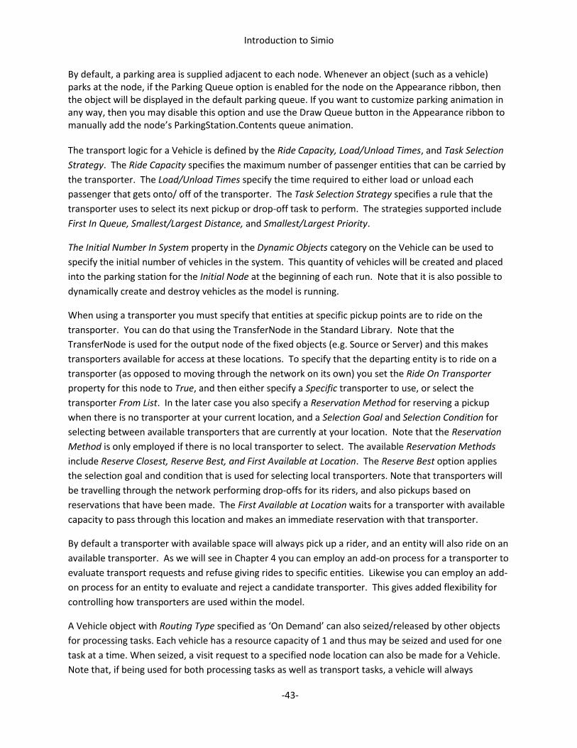
Introduction to Simio
-43-
By default, a parking area is supplied adjacent to each node. Whenever an object (such as a vehicle) parks at the node, if the Parking Queue option is enabled for the node on the Appearance ribbon, then the object will be displayed in the default parking queue. If you want to customize parking animation in any way, then you may disable this option and use the Draw Queue button in the Appearance ribbon to manually add the node’s ParkingStation.Contents queue animation. The transport logic for a Vehicle is defined by the Ride Capacity, Load/Unload Times, and Task Selection
Strategy. The Ride Capacity specifies the maximum number of passenger entities that can be carried by
the transporter. The Load/Unload Times specify the time required to either load or unload each
passenger that gets onto/ off of the transporter. The Task Selection Strategy specifies a rule that the
transporter uses to select its next pickup or drop-off task to perform. The strategies supported include
First In Queue, Smallest/Largest Distance, and Smallest/Largest Priority.
The Initial Number In System property in the Dynamic Objects category on the Vehicle can be used to
specify the initial number of vehicles in the system. This quantity of vehicles will be created and placed
into the parking station for the Initial Node at the beginning of each run. Note that it is also possible to
dynamically create and destroy vehicles as the model is running.
When using a transporter you must specify that entities at specific pickup points are to ride on the
transporter. You can do that using the TransferNode in the Standard Library. Note that the
TransferNode is used for the output node of the fixed objects (e.g. Source or Server) and this makes
transporters available for access at these locations. To specify that the departing entity is to ride on a
transporter (as opposed to moving through the network on its own) you set the Ride On Transporter
property for this node to True, and then either specify a Specific transporter to use, or select the
transporter From List. In the later case you also specify a Reservation Method for reserving a pickup
when there is no transporter at your current location, and a Selection Goal and Selection Condition for
selecting between available transporters that are currently at your location. Note that the Reservation
Method is only employed if there is no local transporter to select. The available Reservation Methods
include Reserve Closest, Reserve Best, and First Available at Location. The Reserve Best option applies
the selection goal and condition that is used for selecting local transporters. Note that transporters will
be travelling through the network performing drop-offs for its riders, and also pickups based on
reservations that have been made. The First Available at Location waits for a transporter with available
capacity to pass through this location and makes an immediate reservation with that transporter.
By default a transporter with available space will always pick up a rider, and an entity will also ride on an
available transporter. As we will see in Chapter 4 you can employ an add-on process for a transporter to
evaluate transport requests and refuse giving rides to specific entities. Likewise you can employ an add-
on process for an entity to evaluate and reject a candidate transporter. This gives added flexibility for
controlling how transporters are used within the model.
A Vehicle object with Routing Type specified as ‘On Demand’ can also seized/released by other objects
for processing tasks. Each vehicle has a resource capacity of 1 and thus may be seized and used for one
task at a time. When seized, a visit request to a specified node location can also be made for a Vehicle.
Note that, if being used for both processing tasks as well as transport tasks, a vehicle will always

Introduction to Simio
-44-
prioritize seize visit requests over any new transport pickup requests. Hence the Vehicle has dual
modes: as a moveable resource (e.g. similar to a worker) that is seized and released and travels from
location to location in the model, and as a transporter that can pickup, carry, and drop off entities at
different locations.
Example: On-Demand Pickups In this example passengers arrive to the system with an inter-arrival time that is exponentially
distributed with a mean of 5 minutes. The passengers are picked up at the arrival point by a vehicle that
can hold up to two passengers at a time, and transports them to the entry location for a service area,
where their service time in minutes has a triangular distribution with a minimum of 1, mode of 2, and
maximum of 3. Once passengers complete service they are then picked up by the same vehicle at the
service area’s exit location and carried to the departure point. The vehicle requires .3 minutes to load or
unload a passenger and can travel 2 meters/second on pathway that has both unidirectional and
bidirectional links as shown below.
Begin by opening Simio and selecting a new model Project. Now drag out a Source, Server, and Sink
and connect them with Paths as shown, changing the Type for Path from the Server to the Sink to
Bidirectional. Edit the Interarrival Time for the Source and Processing Time for the Server, and set the
InputBuffer capacity for the Server to 0 (causing the Server to block the Vehicle on drop-offs).
Now drag an instance of the Vehicle into your model. Set the Initial Node for Vehicle1 to
Output@Source1 and change the Idle Action to None (which causes the Vehicle to sit at its current
location when it goes idle). Also change the Ride Capacity to 2 and set the Load and Unload Time to .3.
Click on the output node at Source1 and add an attached animation queue for ParkingStation.Contents.
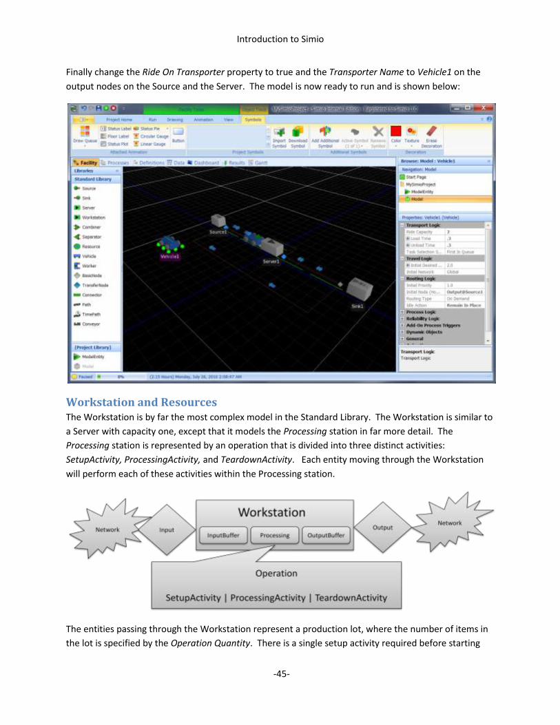
Introduction to Simio
-45-
Finally change the Ride On Transporter property to true and the Transporter Name to Vehicle1 on the
output nodes on the Source and the Server. The model is now ready to run and is shown below:
Workstation and Resources The Workstation is by far the most complex model in the Standard Library. The Workstation is similar to
a Server with capacity one, except that it models the Processing station in far more detail. The
Processing station is represented by an operation that is divided into three distinct activities:
SetupActivity, ProcessingActivity, and TeardownActivity. Each entity moving through the Workstation
will perform each of these activities within the Processing station.
The entities passing through the Workstation represent a production lot, where the number of items in
the lot is specified by the Operation Quantity. There is a single setup activity required before starting
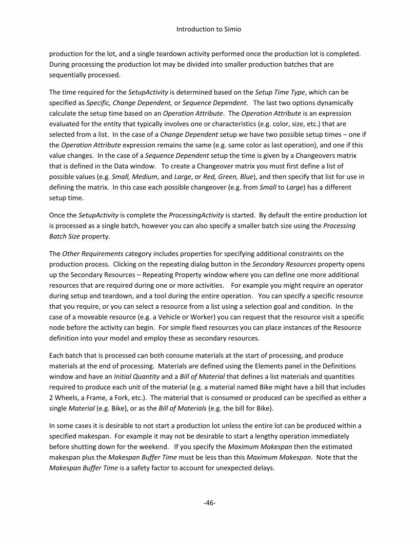
Introduction to Simio
-46-
production for the lot, and a single teardown activity performed once the production lot is completed.
During processing the production lot may be divided into smaller production batches that are
sequentially processed.
The time required for the SetupActivity is determined based on the Setup Time Type, which can be
specified as Specific, Change Dependent, or Sequence Dependent. The last two options dynamically
calculate the setup time based on an Operation Attribute. The Operation Attribute is an expression
evaluated for the entity that typically involves one or characteristics (e.g. color, size, etc.) that are
selected from a list. In the case of a Change Dependent setup we have two possible setup times – one if
the Operation Attribute expression remains the same (e.g. same color as last operation), and one if this
value changes. In the case of a Sequence Dependent setup the time is given by a Changeovers matrix
that is defined in the Data window. To create a Changeover matrix you must first define a list of
possible values (e.g. Small, Medium, and Large, or Red, Green, Blue), and then specify that list for use in
defining the matrix. In this case each possible changeover (e.g. from Small to Large) has a different
setup time.
Once the SetupActivity is complete the ProcessingActivity is started. By default the entire production lot
is processed as a single batch, however you can also specify a smaller batch size using the Processing
Batch Size property.
The Other Requirements category includes properties for specifying additional constraints on the
production process. Clicking on the repeating dialog button in the Secondary Resources property opens
up the Secondary Resources – Repeating Property window where you can define one more additional
resources that are required during one or more activities. For example you might require an operator
during setup and teardown, and a tool during the entire operation. You can specify a specific resource
that you require, or you can select a resource from a list using a selection goal and condition. In the
case of a moveable resource (e.g. a Vehicle or Worker) you can request that the resource visit a specific
node before the activity can begin. For simple fixed resources you can place instances of the Resource
definition into your model and employ these as secondary resources.
Each batch that is processed can both consume materials at the start of processing, and produce
materials at the end of processing. Materials are defined using the Elements panel in the Definitions
window and have an Initial Quantity and a Bill of Material that defines a list materials and quantities
required to produce each unit of the material (e.g. a material named Bike might have a bill that includes
2 Wheels, a Frame, a Fork, etc.). The material that is consumed or produced can be specified as either a
single Material (e.g. Bike), or as the Bill of Materials (e.g. the bill for Bike).
In some cases it is desirable to not start a production lot unless the entire lot can be produced within a
specified makespan. For example it may not be desirable to start a lengthy operation immediately
before shutting down for the weekend. If you specify the Maximum Makespan then the estimated
makespan plus the Makespan Buffer Time must be less than this Maximum Makespan. Note that the
Makespan Buffer Time is a safety factor to account for unexpected delays.
Introduction to Simio
-47-
The estimated makespan is computed based on the shift pattern of the workstation, but does not take
into account shift patterns for secondary resources or material shortages. These are fully accounted for,
however, in the actual makespan for the production lot. Hence it is possible that a production will start
based on its estimated makespan but end up violating the maximum due to constraints.
Worker The Standard Library has a transporter definition named Worker that defines a moveable resource that
may be seized and released for tasks as well as used to transport entities between nodes. A Worker
object is typically used to model operators, doctors, technicians, etc. To use the Worker you drag a
Worker object from the library and place it anywhere in the facility model. You then click on this
Worker object to edit its properties.
In contrast to the Vehicle that supports a Routing Type that can be On Demand or Fixed Route, the
Worker is assumed to always operate in an on demand mode – i.e. the Worker always waits for either a
visit request or a transport request. The Worker always assigns priority to seize visit requests over
transport requests. Unlike the Vehicle, the Worker has the ability to follow a work schedule. When
following a work schedule an Off Shift Action can be specified as Go To Home, Park at Home, Part at
Node, or Remain in Place.
Example: Moveable Operators In this example we have two part types that are produced on separate machines that share a single
operator. PartA has an exponentially distributed inter-arrival time with a mean of 3 minutes, and a
service time in minutes given by a triangular distribution with a minimum of 1 minute, mode of 2
minutes, and a maximum of 3 minutes. . PartB has an exponentially distributed inter-arrival time with a
mean of 4 minutes, and a service time in minutes given by a triangular distribution with a minimum of 1
minute, mode of 2 minutes, and a maximum of 3 minutes. The operator is required for processing on
either machine, and travels at a rate of .5 meters per second over the 10 meter distance between the
machines.
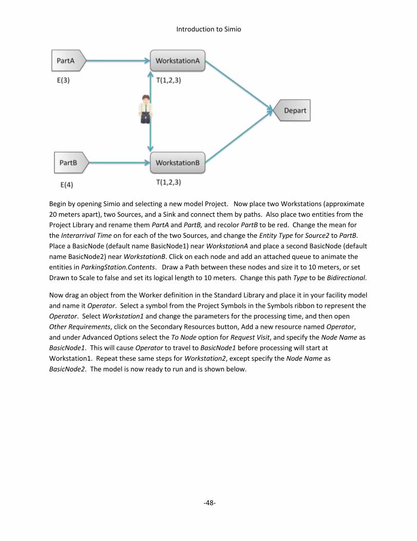
Introduction to Simio
-48-
Begin by opening Simio and selecting a new model Project. Now place two Workstations (approximate
20 meters apart), two Sources, and a Sink and connect them by paths. Also place two entities from the
Project Library and rename them PartA and PartB, and recolor PartB to be red. Change the mean for
the Interarrival Time on for each of the two Sources, and change the Entity Type for Source2 to PartB.
Place a BasicNode (default name BasicNode1) near WorkstationA and place a second BasicNode (default
name BasicNode2) near WorkstationB. Click on each node and add an attached queue to animate the
entities in ParkingStation.Contents. Draw a Path between these nodes and size it to 10 meters, or set
Drawn to Scale to false and set its logical length to 10 meters. Change this path Type to be Bidirectional.
Now drag an object from the Worker definition in the Standard Library and place it in your facility model
and name it Operator. Select a symbol from the Project Symbols in the Symbols ribbon to represent the
Operator. Select Workstation1 and change the parameters for the processing time, and then open
Other Requirements, click on the Secondary Resources button, Add a new resource named Operator,
and under Advanced Options select the To Node option for Request Visit, and specify the Node Name as
BasicNode1. This will cause Operator to travel to BasicNode1 before processing will start at
Workstation1. Repeat these same steps for Workstation2, except specify the Node Name as
BasicNode2. The model is now ready to run and is shown below.
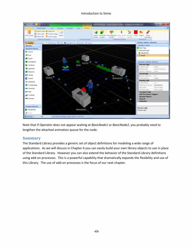
Introduction to Simio
-49-
Note that if Operator does not appear waiting at BasicNode1 or BasicNode2, you probably need to
lengthen the attached animation queue for the node.
Summary The Standard Library provides a generic set of object definitions for modeling a wide range of
applications. As we will discuss in Chapter 6 you can easily build your own library objects to use in place
of the Standard Library. However you can also extend the behavior of the Standard Library definitions
using add-on processes. This is a powerful capability that dramatically expands the flexibility and use of
this Library. The use of add-on processes is the focus of our next chapter.
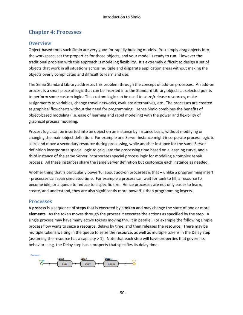
Introduction to Simio
-50-
Chapter 4: Processes
Overview Object-based tools such Simio are very good for rapidly building models. You simply drag objects into
the workspace, set the properties for those objects, and your model is ready to run. However the
traditional problem with this approach is modeling flexibility. It’s extremely difficult to design a set of
objects that work in all situations across multiple and disparate application areas without making the
objects overly complicated and difficult to learn and use.
The Simio Standard Library addresses this problem through the concept of add-on processes. An add-on
process is a small piece of logic that can be inserted into the Standard Library objects at selected points
to perform some custom logic. This custom logic can be used to seize/release resources, make
assignments to variables, change travel networks, evaluate alternatives, etc. The processes are created
as graphical flowcharts without the need for programming. Hence Simio combines the benefits of
object-based modeling (i.e. ease of learning and rapid modeling) with the power and flexibility of
graphical process modeling.
Process logic can be inserted into an object on an instance by instance basis, without modifying or
changing the main object definition. For example one Server instance might incorporate process logic to
seize and move a secondary resource during processing, while another instance for the same Server
definition incorporates special logic to calculate the processing time based on a learning curve, and a
third instance of the same Server incorporates special process logic for modeling a complex repair
process. All these instances share the same Server definition but customize each instance as needed.
Another thing that is particularly powerful about add-on processes is that – unlike a programming insert
- processes can span simulated time. For example a process can wait for tank to fill, a resource to
become idle, or a queue to reduce to a specific size. Hence processes are not only easier to learn,
create, and understand, they are also significantly more powerful than programming inserts.
Processes A process is a sequence of steps that is executed by a token and may change the state of one or more
elements. As the token moves through the process it executes the actions as specified by the step. A
single process may have many active tokens moving thru it in parallel. For example the following simple
process flow waits to seize a resource, delays by time, and then releases the resource. There may be
multiple tokens waiting in the queue to seize the resource, as well as multiple tokens in the Delay step
(assuming the resource has a capacity > 1). Note that each step will have properties that govern its
behavior – e.g. the Delay step has a property that specifies its delay time.

Introduction to Simio
-51-
A process always executes within the context of a parent object. When you create a new process in
your model the parent object is your model. The properties that are specified for each step may
reference properties and states that are “visible” within that context. These properties and states
include those that are owned by the model, as well as objects or elements that have been placed into
the model. If you have objects that contain other elements or objects in their model definition, then
they are also in the context as long as they have been defined with a public scope.
The token that executes a process may also carry its own properties and states. For example a token
might have a state that tracks the number of times the token has passed through a specific point in the
logic. In many cases you can simply use the default token in Simio, however if you require a token with
its own properties and states you can create one in the Token panel within the Definitions window.
A token carries a reference to both its parent object and its associated object (if any). The associated
object is the related object (separate from the parent object) that triggered this process to execute. For
example a process that is triggered by an entity arriving to an object will have that entity as the
associated object. The process logic can reference properties, states, and functions of both the parent
object (i.e. the current model) and the associated object. Hence the token could reference the arriving
entity to specify the delay time on the Delay step. To reference the associated object it is necessary to
precede the property or state name with the object class name. For example ModelEntity.TimeCreated
would return the value of the TimeCreated function for the associated object of type ModelEntity. A
runtime error occurs if the associated object is not the specified type.
The steps in Simio have properties – but do not have states. Hence steps can have input values that
control their behavior, but cannot have variables that change value during the run. The ability to hold
changeable state information is provided by Simio elements. Many of the steps in Simio reference a
specific element (or object, since an object is sub-classed from element). For example the
Consume/Produce steps (which consume and produce material) reference a Material element.
Elements are added to your model using the Elements panel in the Definitions window.
The token also has a ReturnValue that can be assigned during the process. The ReturnValue is typically
used with special processes called decision processes that are executed in zero simulated time (i.e. no
time/status delays – such as a Delay step – are permitted) to make a specific decision. For example a

Introduction to Simio
-52-
process is executed for a Transporter to see if it is willing to accept a new reservation. For a decision
process a ReturnValue of 0 denotes False and a non-zero value denotes True.
Process Types There are three basic types of processes in Simio. All of these processes are built and edited in exactly
the same way and only differ in the mechanism that triggers their execution.
A standard process is a process that is explicitly defined by and executed by the Simio engine. If you
add a standard process to your model you do not have to specify a triggering event since the Simio
engine will automatically execute a standard process at the appropriate time. For example the
OnInitialized standard process is automatically called for each object by the Simio engine during
initialization of the model. You add a standard process to your model by clicking on Select Process icon
in the Process window for the model.
An add-on process is a process that is incorporated into the model of an object to allow the user of that
object to insert their own custom process logic into the model at selected points. The add-on process is
automatically executed within the objects model (using the Execute step), and hence there is no need to
specify a triggering event for the process. The Standard Library makes extensive use of add-on
processes. For example, the Server object provides the following list of add-on processes.
Add-On Process Logical Point in Server Execution
Initialized During initialization of the Server model.
Entered Immediately after an entity enters the Server.
Processing Just before an entity begins processing.
Processed Immediately after an entity completes processing.
Exited Immediately after an entity exits the Server model.
Failed Immediately after the Server enters a failed state.
Repairing Just before the Server is about to start its time to repair time.
Repaired Immediately after the Server returns to a repaired state.
On Shift Immediately after the Server goes on shift.
Off Shift Immediately after the Server goes off shift.
These add-on processes give considerable flexibility in terms of extending the logic executed by the
Server model. For example in the case of the Server the Failed or Repairing add-on process could be
used to seize a repairman, and then the Repaired add-on process could be used to release the
repairman.
There are two ways to insert a new add-on process into the model. The manual way is to click on the
Create Process icon in the Process ribbon for the Processes window, and then select that process for one
of the Add-On Process Triggers in the object that is placed in the facility model. The quick way is to
simply double click on the name of the Add-On Process Trigger, which creates the process with a default
name and then selects that process for that trigger.

Introduction to Simio
-53-
Note that what you are doing with an add-on process is creating a logical process in the context of your
model, and then passing that into an object such as a Server to execute inside that model for that only
that one instance of the Server. The same add-on process can be passed into any number of objects.
An event-triggered process is a process that is triggered by an event that fires within the model. For
example a station element named Input (which might be used to define an input station within the
object) fires an Input.Entered event each time the Input station is entered. You can have a process be
triggered to execute by this event by specifying the Triggering Event property for the process as
Input.Entered. A token will then execute this process each time an entity enters the station, and the
associated object for the token will be the entering entity. It is also possible to have multiple triggering
events and to dynamically change the triggering event during the running of the simulation by using the
Subscribe and Unsubscribe steps in the process logic.
You create an event-triggered process by clicking on the Create Process icon in the Process tab of the
Processes window, and then specify the Triggering Event property for that process.
Building Processes You build and edit processes using the Process window shown below. The left side of this window has a
fly-out panel for selecting steps, and the right hand side has the navigation panel and properties editor.
The steps are categorized by Common Steps, All Steps, and User Defined Steps. The Common steps
include the steps that are most frequently used in models. The All Steps include all of the built-in steps
for Simio. The User-Defined Steps include user-coded steps that have been added to Simio to extend
the core functionality of the product (for details see the Simio User-Extensions Reference Guide).

Introduction to Simio
-54-
When a new process is added to the window it is shown with a Begin and End point and no steps in
between. You add steps to the process by dragging them out from the panel and dropping them at the
desired location. Simio incorporates a layout tool that automatically redraws the process as you drop
each new step. You can drag a step to move it to a new location within the layout. You can also drag
one of the End points to connect it to the input of step. The following shows the result of the automatic
layout with multiple Decide steps, where the End coming out of the Delay step has been connected to
the input side of the Assign.
You select a step by clicking on the step, and you select the process by clicking outside the steps. If you
select a step the properties of the step are displayed in the Property window. If change the properties
of a step from their default values and then hover over the step a box will appear showing the non-
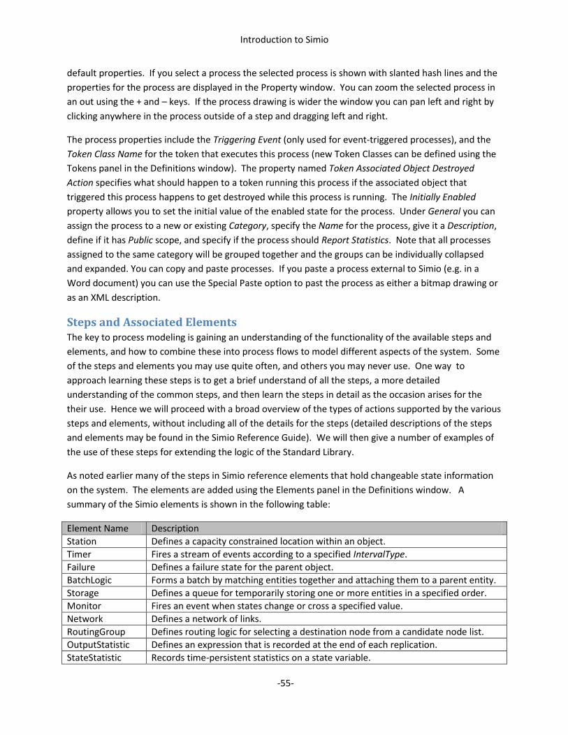
Introduction to Simio
-55-
default properties. If you select a process the selected process is shown with slanted hash lines and the
properties for the process are displayed in the Property window. You can zoom the selected process in
an out using the + and – keys. If the process drawing is wider the window you can pan left and right by
clicking anywhere in the process outside of a step and dragging left and right.
The process properties include the Triggering Event (only used for event-triggered processes), and the
Token Class Name for the token that executes this process (new Token Classes can be defined using the
Tokens panel in the Definitions window). The property named Token Associated Object Destroyed
Action specifies what should happen to a token running this process if the associated object that
triggered this process happens to get destroyed while this process is running. The Initially Enabled
property allows you to set the initial value of the enabled state for the process. Under General you can
assign the process to a new or existing Category, specify the Name for the process, give it a Description,
define if it has Public scope, and specify if the process should Report Statistics. Note that all processes
assigned to the same category will be grouped together and the groups can be individually collapsed
and expanded. You can copy and paste processes. If you paste a process external to Simio (e.g. in a
Word document) you can use the Special Paste option to past the process as either a bitmap drawing or
as an XML description.
Steps and Associated Elements The key to process modeling is gaining an understanding of the functionality of the available steps and
elements, and how to combine these into process flows to model different aspects of the system. Some
of the steps and elements you may use quite often, and others you may never use. One way to
approach learning these steps is to get a brief understand of all the steps, a more detailed
understanding of the common steps, and then learn the steps in detail as the occasion arises for the
their use. Hence we will proceed with a broad overview of the types of actions supported by the various
steps and elements, without including all of the details for the steps (detailed descriptions of the steps
and elements may be found in the Simio Reference Guide). We will then give a number of examples of
the use of these steps for extending the logic of the Standard Library.
As noted earlier many of the steps in Simio reference elements that hold changeable state information
on the system. The elements are added using the Elements panel in the Definitions window. A
summary of the Simio elements is shown in the following table:
Element Name Description
Station Defines a capacity constrained location within an object.
Timer Fires a stream of events according to a specified IntervalType.
Failure Defines a failure state for the parent object.
BatchLogic Forms a batch by matching entities together and attaching them to a parent entity.
Storage Defines a queue for temporarily storing one or more entities in a specified order.
Monitor Fires an event when states change or cross a specified value.
Network Defines a network of links.
RoutingGroup Defines routing logic for selecting a destination node from a candidate node list.
OutputStatistic Defines an expression that is recorded at the end of each replication.
StateStatistic Records time-persistent statistics on a state variable.

Introduction to Simio
-56-
TallyStatistic Holds summary statistics for observational values recorded using a Tally step.
Operation Defines a sequence of activities that are preformed over time.
Activity Defines an activity that is performed within an operation.
Material Defines a material that can be produced or consumed and own a bill of material.
Most of the steps are general purpose steps that can be used by any of the five object types. However
some steps are specific to a specific object type such as an entity, transporter, node, or link.
We will begin first describing the general purpose steps which are summarized in the following table.
Note that the shaded steps are those included in the Common Steps list and are the ones most often
used. Where appropriate the elements that are referenced by the steps are also noted. Elements are
added to the model using the Elements panel in the Definitions window.
General Purpose Steps
Step Name Action
Assign Assigns an expression value to a state variable.
Decide Sends the token to one of two exit points based on an expression.
Delay Delays the token for a specified time.
Execute Executes a process and either waits or continues.
Tally Tallies a value in the specified TallyStatistic element.
Create Creates a new entity.
Destroy Destroys the parent or associated entity.
Fire Fires the specified object event.
Wait Waits for a specified event to fire.
Seize Seizes one or more resource objects.
Release Releases one or more resource objects.
Transfer Transfers the associated entity between objects and/or free space or between stations.
EndTransfer Completes the transfer of the associated entity into the object and/or station.
Allocate Manually trigger resource allocation for the parent object.
Batch Create a batch with the associated entity using the BatchLogic element.
Consume Consume a specified quantity of material.
EndActivity End the current operation activity for the associated entity.
EndOperation End the current operation for an entity.
Fail Specifies a Failure element to change to a failed state.
Insert Insert the associated or parent object into a queue.
Interrupt Maybe be used to interrupt process delays.
Produce Produces a specified quantity of a material.
Remove Remove the associated or parent object from a queue.
Repair Specifies a Failure element to restore to a repaired state.
Resume Resumes a suspended process or movement of the parent or associated object.
Search Search a collection of items including table rows or objects in a list or queue.
SetNetwork Sets the current network for the parent or associated object.
SetNode Sets the current destination for the parent or associated object.
SetTable Sets a table reference and row for the token or parent/associated object.
Introduction to Simio
-57-
The Assign step is used to assign an expression value to one or more state variables. The Assign step
displays a single assignment in the main properties grid, but allows for additional assignments in the
Repeating Properties Editor.
The assignment action is to evaluate the specified Value expression, and assign that value to the
specified State Variable Name. A state variable may be added to your model by selecting the States
panel in the Definitions window for the model and then clicking on one of the four state icons in the
States ribbon. Note that a state added to your main model can be thought of as a global variable, while a
state added to an entity model or other object may be thought of as an attribute of that entity or object.
A discrete state is the most commonly used state variable and can be assigned any real value. By
default a discrete state variable is a simple Scalar, but it can also be dimensioned as a Vector, a Matrix,
or an array up to 10 dimensions. In the later case you enter a number for Dimensions instead of
selecting from the drop list. In the case of a vector or matrix you can also both dimension and initialize a
state variable using the values in a data table by selecting the Dimensions property as [Table]. In this
case the number of rows and columns for the matrix are set to the number of rows and columns in the
table, and the matrix is initialized to the table values. As we will see in Chapter 5 this is a very
convenient way to both dimension and initialize arrays using external data.
A level state is a variable that is described by both a rate and level. For example if you create a level
state named Tank, you can reference the level value by Tank, and the corresponding rate value by
Tank.Rate. Note that the Tank value automatically updates based on the current value assigned to
Tank.Rate.
A movement state is a state that can have a rate, acceleration, acceleration duration, heading between
0 and 360 degrees, and a pitch relative to the floor measured in degrees. If you create a movement
state variable named Travel, then the value Travel will be the total distance traveled, and the values for
Travel.Rate, Travel.Acceleration, Travel.AccelerationDuration, Travel.Heading, and Travel.Pitch will be
the related parameters for the state.
A list state is a state variable that can be assigned a value from a list (list are defined using the List panel
in the Definitions Window). For example a list named Color with members Red, Green, Blue could be
used to define a list state name ColorValue. The numeric value of a list is referenced using the keyword
List. Hence assigning ColorValue to List.Color.Blue would set ColorValue to the color list member Blue.
All state values return a numeric and in the case of a list state this is the zero-based index into the list, or
in this case a value 2 since Blue is a zero-based index 2.
StartActivity Starts a specified activity for an operation.
StartOperation Starts a specified operation.
Subscribe Adds a new triggering event to a process.
Suspend Suspends a process or movement of the parent or associated object.
UnSubscribe Removes a triggering event for a process.

Introduction to Simio
-58-
Note that if you are adding state variables to one more entity models, and then creating objects for
those entities, you must reference the states of the entity by prefixing the state names with the entity
model name. For example if you create an entity model named Part, and then give it discrete states X
and Y, you reference these states as Part.X and Part.Y.
In addition to the Assign step, there are several other steps used to set dynamic characteristic of an
entity/object including SetNetwork (specifies the network to follow), SetNode (specifies the destination
to travel towards), and SetTable (specifies a row in a data table for retrieving data).
The Decide step is used to select one of two exit points based on the value of an expression. The
expression is interpreted either as a logical condition or a probability based on the Decide Type
property.
The Delay step is used to delay the token by a specified time. This step is typically used to model
general processing delays in the system.
The Execute step is used to execute another process. This step will either hold the current token until
the specified process is completed, or continue and execute in parallel to the spawned process.
The Tally step is used to record a value for a specified TallyStatistic element. To use the Tally step you
must first add a TallyStatistic element to your model. The Tally can record either the value of an
expression, or the time between arrivals to the TallyStatistic based on the Value Type property specified
for the step. Note that Token.TimeInProcess can be used in the expression to record the time that the
token has spent in the process, and Entity.TimeInSystem can be used in the expression to record the
time that the associated entity has spent in the system.
The Create and Destroy steps are used to create and destroy dynamic objects which include entities and
transporters. The Create can either create a new dynamic object, or create a copy of either the parent
object or associated object. The Destroy step can destroy either the associated object or the parent
object (i.e. destroy itself).
The Fire and Wait steps provide coordination between logical points within an object, or between
objects. The Fire step is used to fire an event that has been defined for the object (events are defined
using the Events panel in the Definitions window). The Wait step is used to hold an entity until a
specified event has been fired. The Wait step also includes a Release Condition property that if specified
must be true for a token to be released.
The Seize and Release steps are used to seize and release capacity of an object that has been defined as
a resource. As noted in Chapter 3 that Resource object can be used to model fixed resources, and the
Vehicle object or an Operator entity can be used to model a moveable resource. Both the Seize and
Release steps utilize the Repeat Group Editor to allow for multiple seizes and releases at a single step.
Note that in the case of the Seize you can request a visit by a moveable resource using the Request Visit
property under Advanced options.
Introduction to Simio
-59-
The Transfer and EndTransfer steps are used to initiate and complete entity transfers between objects,
between an object and free space, or between stations within an object. At the completion of the
transfer the EndTransfer step fires the entity’s Transferred event. These steps are used to provide a
“handshake” between objects in the model. We will discuss the use of these steps in detail in Chapter 6
where we discuss building custom objects.
There are a number of steps that are specific to modeling the behavior of entities and transporters.
Since the transporter is sub-classed from entity, any of the entity steps can also be used within the
model of a transporter. These steps are shown below:
Entity Steps
Step Name Action
Arrive Notifies the visit request that the entity has arrived to the requested location.
PlanVisit Search for and accept a ride pickup or visit request as a planned node visit.
SelectVisit Select a planned node visit and set the destination to the selected node.
Transporter Steps
Step Name Action
Dropoff Drop off a passenger entity at the current node.
Pickup Pickup a passenger entity from the RidePickupQueue at the current node.
SelectDropoff Set the destination to a selected passenger entity in the RideQueue.
There are also a number of steps that are used for modeling the behavior of a node object. Note that
the Park and UnPark steps can also be used within a model of an entity or transporter by referencing
the parent object rather than the associated object.
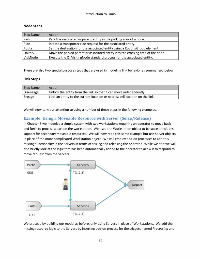
Introduction to Simio
-60-
Node Steps
Step Name Action
Park Park the associated or parent entity in the parking area of a node.
Ride Initiate a transporter ride request for the associated entity.
Route Set the destination for the associated entity using a RoutingGroup element.
UnPark Move the parked parent or associated entity into the crossing area of the node.
VisitNode Execute the OnVisitingNode standard process for the associated entity.
There are also two special purpose steps that are used in modeling link behavior as summarized below:
Link Steps
Step Name Action
Disengage Unlock the entity from the link so that it can move independently.
Engage Lock an entity to the current location or nearest cell location on the link.
We will now turn our attention to using a number of these steps in the following examples.
Example: Using a Moveable Resource with Server (Seize/Release) In Chapter 3 we modeled a simple system with two workstations requiring an operator to move back
and forth to process a part on the workstation. We used the Workstation object to because it includes
support for secondary moveable resources. We will now redo this same example but use Server objects
in place of the more complicated Workstation object. We will employ add-on processes to add this
missing functionality in the Servers in terms of seizing and releasing the operator. While we at it we will
also briefly look at the logic that has been automatically added to the operator to allow it to respond to
move request from the Servers.
We proceed by building our model as before, only using Servers in place of Workstations. We add the
missing resource logic to the Servers by inserting add-on process for the triggers named Processing and

Introduction to Simio
-61-
Processed. The Processing trigger occurs immediately before processing begins, and the Processed
trigger occurs immediately after processing is completed. We will add a Seize step to each Processing
add-on process, and a Release step to each Processed add-on process, as shown below.
On the Seize steps we specify Operator as the resource to seize, and under the Advanced Options we
specify a visit request to BasicNode1 for ServerA, and BasicNode2 for ServerB. On the Release step we
specify Operator as the resource to release. The model is now ready to run and is shown below:

Introduction to Simio
-62-
Summary The chapter has introduced the concept of process logic for adding new behaviors to our existing
modeling objects. The ability to insert process logic into individual instances of an object is an extremely
powerful capability in Simio. In Chapter 6 we will expand further on these concepts when we discuss
process concepts for building object libraries.
Introduction to Simio
-63-
Chapter 5: Data Driven Models
Overview Simulation models typically have data that is used to drive the model. In some cases this data is
conveniently entered directly into the modeling objects. For example with simple flow line making a
single part it might be convenient to “hard code” the inter-arrival time and processing times directly into
the properties for the objects in the model. However in many cases there is a large amount of data as
well as a desire to frequently change the data. In addition the people using the model with different
sets of data may not be the same person that builds the model. In these cases it is convenient to be
able to define the data in data tables and then have the model reference the data in those tables. It
may also be desirable to either import or directly bind the data tables to external data sources such as
Excel or a database. This chapter describes the features in Simio for building data-driven models using
data tables that interface to external data sources.
Data Tables A Simio data table is a data container that has a collection of user-defined columns with corresponding
rows of data. Each column can hold a specific type of data such as a string, real number, Boolean, date-
time, expression value, entity type, etc. Within Simio you can define as many tables as you like, and
each table can have any number of columns of different types. You can create relations between tables
such that an entry in one table can reference the data held by another table. For example a table of
production orders could reference a table of product descriptions.
A data table is defined using the Tables panel in the Data window. To add a new table you click on
either Data Table or Sequence Table in the Tables section of the Table ribbon. The sequence table is
data table with a column named Sequence that has already been added to the table for specifying a
routing sequence for an entity. Hence everything that applies to a data table also applies to sequence
tables. Once you have added a table you can rename it and give it a description by clicking on the tab for
the table and then setting the table properties in the Property window.
If you add multiple tables you can drag the tabs apart and drop them on the layout targets to arrange
them as you wish. You can also arrange them into vertical and horizontal tab groups by right clicking
any table tab and selecting the appropriate option.
To add columns to a table you select a table to make it active and then click on property types under
Standard Property, Element Reference, Object Reference, or Foreign Key. You can then rename the
column by selecting the column header and changing the column properties. An element reference is a
reference to a Simio element such as a Station or Material. An object reference is a reference to an
object instance such as Worker or Lathe. The standard properties are all the other property types in
Simio and include the following:

Introduction to Simio
-64-
Property Type Description
Real A real constant: e.g. 132.7
Integer An integer constant: e.g. 34 or -27
Boolean A true/false check box.
Expression A valid Simio expression involving one or more variables: e.g. (X + Y) / 2.3
Date Time A date time value with a calendar date selector: e.g. 1/1/2010 12:00:00 AM
String A valid string: e.g. Fred
Event An event that is defined in the context of the model: e.g. ModelEntity.Transferred
List A value selected from a list that is referenced by the property: e.g. Red
Enumeration A value from an enumeration that is referenced by the property: e.g. FirstInFirstOut
Rate Table A rate table that is defined for this model: e.g. ArrivalPattern
Table A data table that is defined for this model: e.g. ProductTable
Sequence Table A sequence table that is defined for this model: e.g. RoutingTable
State A state that is defined for this model: e.g. ReworkCount
Schedule A schedule that is defined for this model: e.g. OverTimeShift
Selection Rule A dynamic selection rule: e.g. Smallest Value First
Note that some properties have required values that must be set in the Properties Editor for the column
to work. For example a List property requires that a list specified that defines the valid options for the
column. Hence we create a list named Colors with value members Red, Green, and Blue, and then add a
List column referencing the Colors list; the valid entries for the column are Red, Green, and Blue.
The columns that specify numeric values (e.g. Real, Integer, Expression) also have a Unit Type property
that can be specified. The unit type can be Time, Travel Rate, or Length, and then the appropriate units
can be specified (e.g. Meters, Feet per Minute, etc.).
You can also select a column and make it a Key Column. A key column must have all unique entries in
the column. For example a key column of type Integer cannot have two rows with the same number. A
key column can then be referenced by adding a Foreign Key column property in another table, and
referencing this table and key column in the properties of the foreign key. This will then link the rows in
that table to a row in this table using the unique key value in this column. We will see an example of
this later in this chapter.
The following shows an example table named MyTable with four columns named W, X, Y, Z. Column W
is a real column with Unit Type specified as Time and units in Hours. Column X is a Boolean column
where a check mark indicates True. A Boolean True in Simio has a numeric value of 1. Column Y is a
string column and is set as a key column as indicated by the yellow column header. As a result the string
entries in this column must be unique. Column Z is an expression column and accepts any valid Simio
expression.
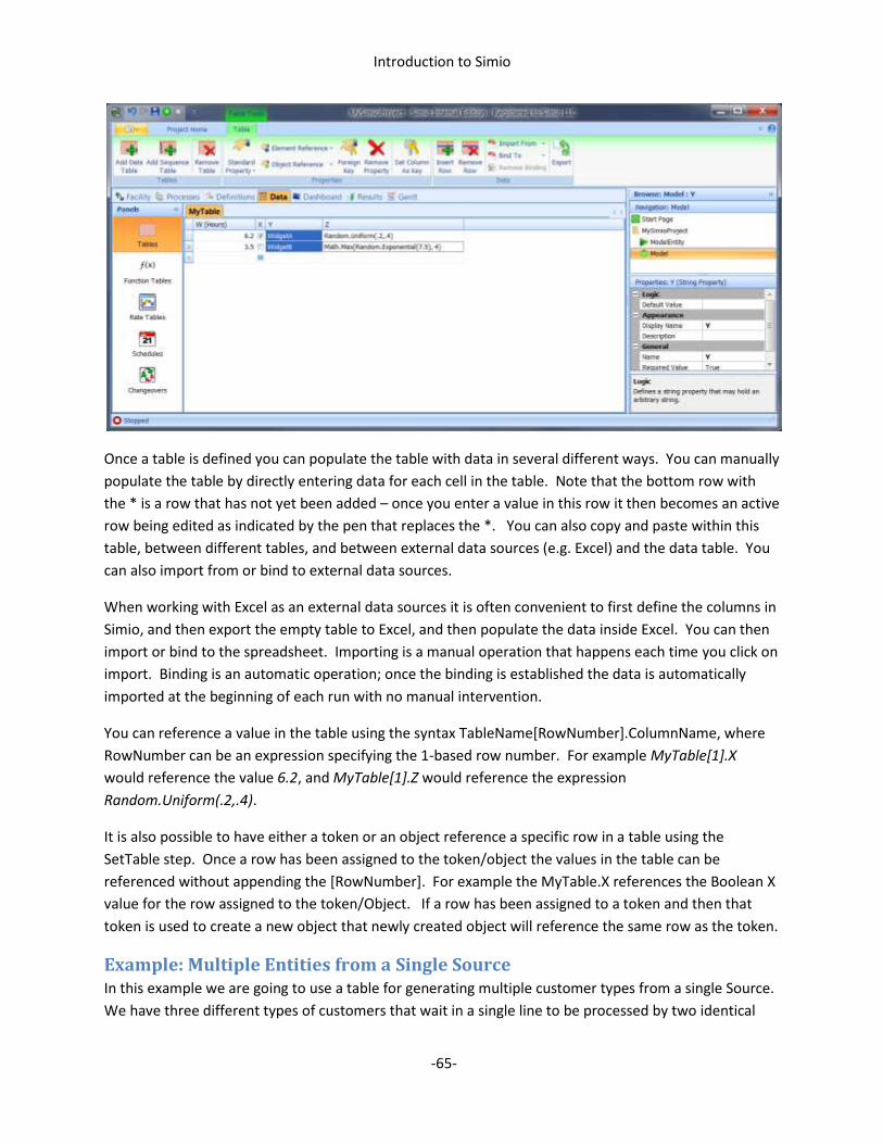
Introduction to Simio
-65-
Once a table is defined you can populate the table with data in several different ways. You can manually
populate the table by directly entering data for each cell in the table. Note that the bottom row with
the * is a row that has not yet been added – once you enter a value in this row it then becomes an active
row being edited as indicated by the pen that replaces the *. You can also copy and paste within this
table, between different tables, and between external data sources (e.g. Excel) and the data table. You
can also import from or bind to external data sources.
When working with Excel as an external data sources it is often convenient to first define the columns in
Simio, and then export the empty table to Excel, and then populate the data inside Excel. You can then
import or bind to the spreadsheet. Importing is a manual operation that happens each time you click on
import. Binding is an automatic operation; once the binding is established the data is automatically
imported at the beginning of each run with no manual intervention.
You can reference a value in the table using the syntax TableName[RowNumber].ColumnName, where
RowNumber can be an expression specifying the 1-based row number. For example MyTable[1].X
would reference the value 6.2, and MyTable[1].Z would reference the expression
Random.Uniform(.2,.4).
It is also possible to have either a token or an object reference a specific row in a table using the
SetTable step. Once a row has been assigned to the token/object the values in the table can be
referenced without appending the [RowNumber]. For example the MyTable.X references the Boolean X
value for the row assigned to the token/Object. If a row has been assigned to a token and then that
token is used to create a new object that newly created object will reference the same row as the token.
Example: Multiple Entities from a Single Source In this example we are going to use a table for generating multiple customer types from a single Source.
We have three different types of customers that wait in a single line to be processed by two identical

Introduction to Simio
-66-
servers. The customers arrive according to a Poisson process, with a mean time between arrivals that is
exponentially distributed with a mean of 3 minutes. The customer mix (percentage) and the processing
time on the server are summarized in the following table.
Customer Type Mix (Percentage) Processing Time
Standard 60 Random.Triangular(3,4,5)
Simple 15 Random.Triangular(1,2,3)
Complex 25 Random.Triangular(7,9,12)
To model this we will place a Source, Server, and Sink into our facility and connect them with Paths with
Allow Passing set to False. We will specify the time between arrivals for the Source as an exponential
sample with a mean of 3 minutes, and we will set Input Buffer on the Server to 0, and set the Capacity to
2. The combination of no input buffer on the Server and no passing on the Path will cause our
customers to queue up along the path in front of the Server. The capacity of 2 on the Server will allow
this single Server object to represent two identical servers. We also place three instances of
ModelEntity and rename them Standard, Simple, and Complex, and select people symbols from the
symbol library to represent these three customer types.
We will now build a Simio table by selecting the Data window and clicking on Add Data Table and then
renaming the table CustomerData. Next we will add a column named CustomerType by clicking on the
Object Reference property and selecting Entity. Next we add a column named Mix by clicking on
Standard Property and selecting Real. We then add a column named ProcessTime by clicking on
Standard Property and selecting Expression. We also set the Unit Type for this property to Time and set
the units to Minutes. We then manually enter the data for the table as shown below:

Introduction to Simio
-67-
Now that we have this table defined we will use it to select the type of entity to create at the Source,
and specify the processing time at the Server. To do this we will specify a table reference assignment for
our Source object Before Creating Entities. We will specify the Table Name as CustomerData, and
specify the Row Number as CustomerData.Mix.RandomRow. Note that RandomRow is a function that
returns a random row number based on the values in the Mix column as weights. We can specify the
Entity Type as CustomerData.CustomerType. The newly created entity will then point to this same row.
We then change the processing time for the Server to be CustomerData.ProcessTime. Hence the
processing time will be taken from the ProcessTime column for the selected row.
The running model for this example is shown below. Note that you may need to lengthen the
Processing.Contents animation queue to see both customers in service at the same time.
This example is simple but illustrates the power of tables for building data driven models. Note that we
could also bind this table to an Excel spreadsheet and then do all of our data editing in the spreadsheet.
Example: Product Routings using Separate Sequence Tables In this example we have three part types with each part type having a different routing through a facility
comprised of three servers. The product mix for the three part types is 20% type A, 30% type B, and
50% type C. The routing and processing time for each of the three part types is summarized in the
following tables:
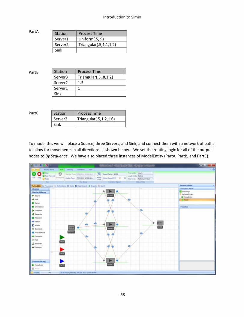
Introduction to Simio
-68-
PartA
PartB
PartC
To model this we will place a Source, three Servers, and Sink, and connect them with a network of paths
to allow for movements in all directions as shown below. We set the routing logic for all of the output
nodes to By Sequence. We have also placed three instances of ModelEntity (PartA, PartB, and PartC).
Station Process Time
Server1 Uniform(.5,.9)
Server2 Triangular(.5,1.1,1.2)
Sink
Station Process Time
Server3 Triangular(.5,.8,1.2)
Server2 1.5
Server1 1
Sink
Station Process Time
Server2 Triangular(.5,1.2,1.6)
Sink
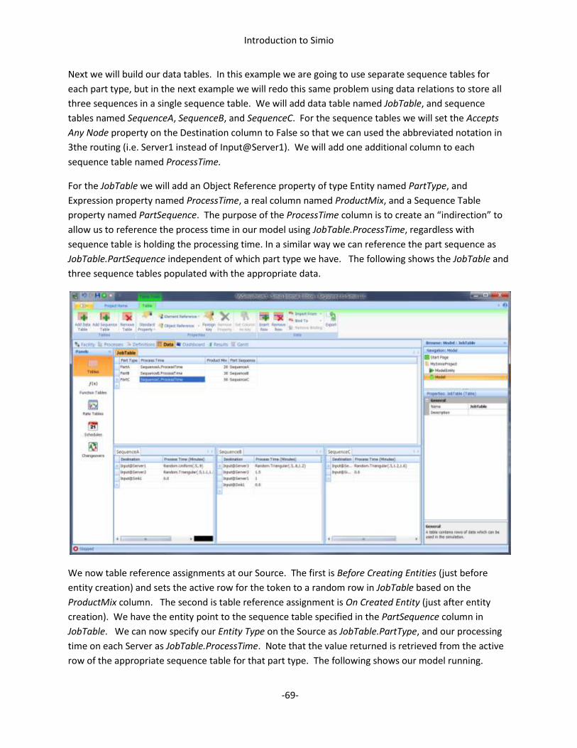
Introduction to Simio
-69-
Next we will build our data tables. In this example we are going to use separate sequence tables for
each part type, but in the next example we will redo this same problem using data relations to store all
three sequences in a single sequence table. We will add data table named JobTable, and sequence
tables named SequenceA, SequenceB, and SequenceC. For the sequence tables we will set the Accepts
Any Node property on the Destination column to False so that we can used the abbreviated notation in
3the routing (i.e. Server1 instead of Input@Server1). We will add one additional column to each
sequence table named ProcessTime.
For the JobTable we will add an Object Reference property of type Entity named PartType, and
Expression property named ProcessTime, a real column named ProductMix, and a Sequence Table
property named PartSequence. The purpose of the ProcessTime column is to create an “indirection” to
allow us to reference the process time in our model using JobTable.ProcessTime, regardless with
sequence table is holding the processing time. In a similar way we can reference the part sequence as
JobTable.PartSequence independent of which part type we have. The following shows the JobTable and
three sequence tables populated with the appropriate data.
We now table reference assignments at our Source. The first is Before Creating Entities (just before
entity creation) and sets the active row for the token to a random row in JobTable based on the
ProductMix column. The second is table reference assignment is On Created Entity (just after entity
creation). We have the entity point to the sequence table specified in the PartSequence column in
JobTable. We can now specify our Entity Type on the Source as JobTable.PartType, and our processing
time on each Server as JobTable.ProcessTime. Note that the value returned is retrieved from the active
row of the appropriate sequence table for that part type. The following shows our model running.
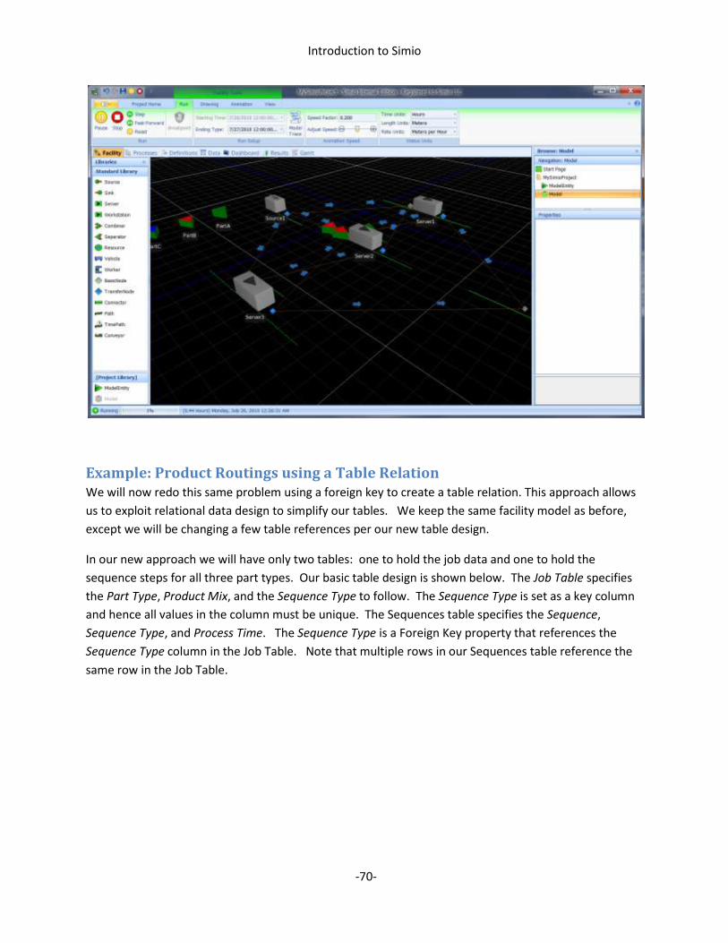
Introduction to Simio
-70-
Example: Product Routings using a Table Relation We will now redo this same problem using a foreign key to create a table relation. This approach allows
us to exploit relational data design to simplify our tables. We keep the same facility model as before,
except we will be changing a few table references per our new table design.
In our new approach we will have only two tables: one to hold the job data and one to hold the
sequence steps for all three part types. Our basic table design is shown below. The Job Table specifies
the Part Type, Product Mix, and the Sequence Type to follow. The Sequence Type is set as a key column
and hence all values in the column must be unique. The Sequences table specifies the Sequence,
Sequence Type, and Process Time. The Sequence Type is a Foreign Key property that references the
Sequence Type column in the Job Table. Note that multiple rows in our Sequences table reference the
same row in the Job Table.
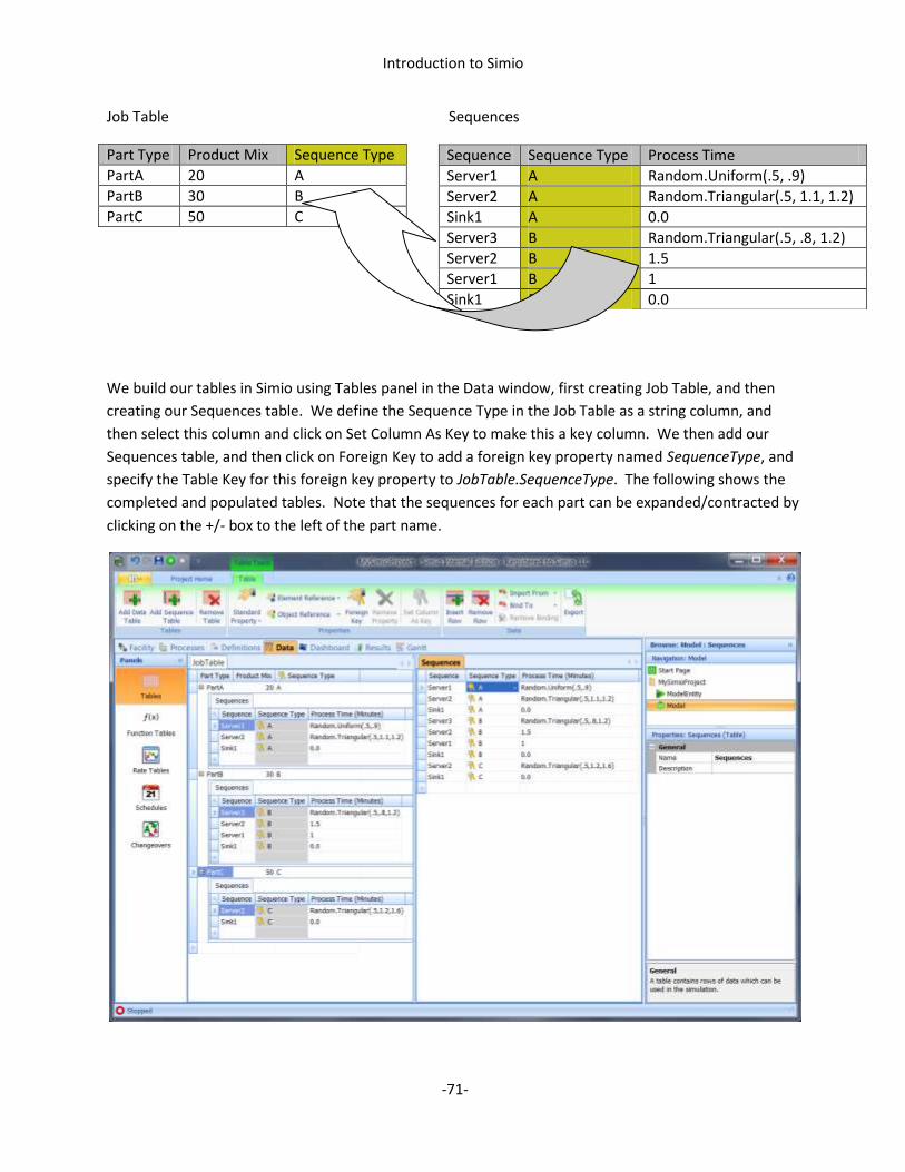
Introduction to Simio
-71-
Job Table Sequences
Part Type Product Mix Sequence Type
PartA 20 A
PartB 30 B
PartC 50 C
We build our tables in Simio using Tables panel in the Data window, first creating Job Table, and then
creating our Sequences table. We define the Sequence Type in the Job Table as a string column, and
then select this column and click on Set Column As Key to make this a key column. We then add our
Sequences table, and then click on Foreign Key to add a foreign key property named SequenceType, and
specify the Table Key for this foreign key property to JobTable.SequenceType. The following shows the
completed and populated tables. Note that the sequences for each part can be expanded/contracted by
clicking on the +/- box to the left of the part name.
Sequence Sequence Type Process Time
Server1 A Random.Uniform(.5, .9) Server2 A Random.Triangular(.5, 1.1, 1.2) Sink1 A 0.0 Server3 B Random.Triangular(.5, .8, 1.2) Server2 B 1.5 Server1 B 1 Sink1 B 0.0
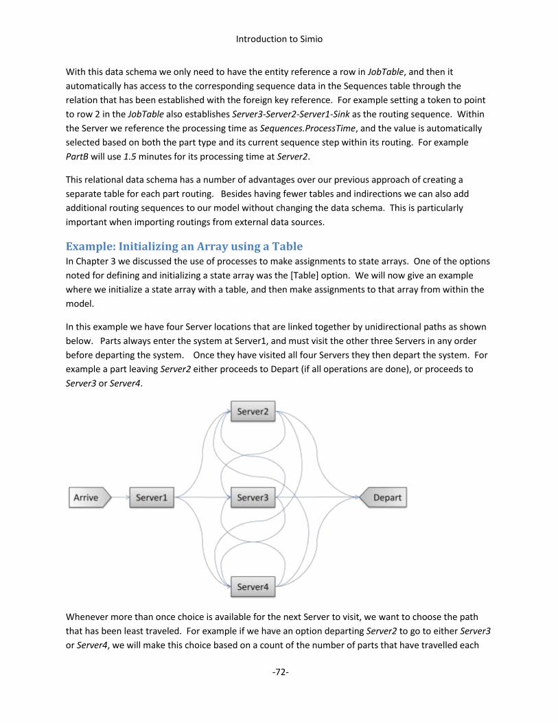
Introduction to Simio
-72-
With this data schema we only need to have the entity reference a row in JobTable, and then it
automatically has access to the corresponding sequence data in the Sequences table through the
relation that has been established with the foreign key reference. For example setting a token to point
to row 2 in the JobTable also establishes Server3-Server2-Server1-Sink as the routing sequence. Within
the Server we reference the processing time as Sequences.ProcessTime, and the value is automatically
selected based on both the part type and its current sequence step within its routing. For example
PartB will use 1.5 minutes for its processing time at Server2.
This relational data schema has a number of advantages over our previous approach of creating a
separate table for each part routing. Besides having fewer tables and indirections we can also add
additional routing sequences to our model without changing the data schema. This is particularly
important when importing routings from external data sources.
Example: Initializing an Array using a Table In Chapter 3 we discussed the use of processes to make assignments to state arrays. One of the options
noted for defining and initializing a state array was the [Table] option. We will now give an example
where we initialize a state array with a table, and then make assignments to that array from within the
model.
In this example we have four Server locations that are linked together by unidirectional paths as shown
below. Parts always enter the system at Server1, and must visit the other three Servers in any order
before departing the system. Once they have visited all four Servers they then depart the system. For
example a part leaving Server2 either proceeds to Depart (if all operations are done), or proceeds to
Server3 or Server4.
Whenever more than once choice is available for the next Server to visit, we want to choose the path
that has been least traveled. For example if we have an option departing Server2 to go to either Server3
or Server4, we will make this choice based on a count of the number of parts that have travelled each

Introduction to Simio
-73-
path. We will keep this count in an array that we wish to initialize with an initial count as follows, and
then bump by 1 each time we travel the path.
From/To Server1 Server2 Server3 Server4
Server1 0 12 16 13
Server2 0 0 14 10
Server3 0 17 0 15
Server4 0 9 8 0
We will begin by building our facility model. We place a Source, 4 Servers, and a Sink, and then connect
them with paths as shown below:
Next we will define our data table for initializing our PathCount state array. We add a data table named
PathTable and create real-valued columns named Server1, Server2, Server3, and Server4, and then
populate this table with counts for each travel path as follows:
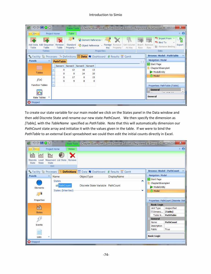
Introduction to Simio
-74-
To create our state variable for our main model we click on the States panel in the Data window and
then add Discrete State and rename our new state PathCount. We then specify the dimension as
[Table], with the TableName specified as PathTable. Note that this will automatically dimension our
PathCount state array and initialize it with the values given in the table. If we were to bind the
PathTable to an external Excel spreadsheet we could then edit the initial counts directly in Excel.

Introduction to Simio
-75-
When departing Server1 we will make our select our next destination based on the smallest current
count for the three outgoing paths using the following process logic in the Output node at Server1. If
the path count from Server1 to Server2 is less than the current count to both Server3 and Server4 we
select Server2, otherwise we select between Server3 and Serve4 based on the smallest path count. We
enter the expression for Path2 <= Path3&4 as:
PathCount[1,2] <= Math.Min(PathCount[1,3], PathCount[1,4]).
To support the destination selection logic at Servers 2, 3, and 4 we will keep a count on the number of
Servers visited by each part, as well as the index of the last Server visited. We select our ModelEntity
and click on the States panel in its Definition window and add a Discrete State named LastServer. For
the number of Servers visited we will make use of the existing Picture state variable on ModelEntity. We
will bump this value by 1 each time a the part leaves Server 2, 3, or 4, and then use a Green, Red, Blue,
and Yellow entity symbol animate the number of Servers that have been visited by each part.
When departing Server2 we will use the following process logic.
We first increment the Picture state variable and then check if the server count is equal to four. Note
that this expression is entered as ModelEntity.Picture == 3 since we are using the Picture state for a dual
purpose: to set the zero-based symbol index, and to track number of servers completed (not counting
Server 1). The expression for LastServer == 3 is entered as ModelEntity.LastServer == 3.
If the server count for this part is 4 (i.e. ModelEntity.Picture == 3) we go straight to Depart. Otherwise if
the server count is 3 we select between Server3 and Server4 to avoid revisiting the same Server again as
our last Server. Otherwise we have yet to visit either Server3 or Server4 so we select between them

Introduction to Simio
-76-
based on the travel path count. Note that this logic will ensure that we visit each Server exactly once.
We define similar logic for selecting our next destination at Server3 and Server4.
We add the decision processes to the Entered add-on process for the output node on each of the
Servers. We also add a small assignment process to each of the Exited add-on processes on the output
nodes for Server2, Server3, and Server4 to update ModelEntity.LastServer to 2, 3, and 4 respectively.
Finally we add a small assignment process for the Entered process trigger to each of the paths
connecting the four servers to update the path count. For example the path connecting Server2 to
Server3 we increment PathCount[2,3] by 1. We are now ready to run which produces the following
animated model.
Summary This chapter has reviewed the basic concepts for creating data driven models. The table features of
Simio can be used to create models that obtain their input data from Excel spreadsheets and other
external data sources making it very easy to manipulate the data for the model.

Introduction to Simio
-77-
Chapter 6: Object Definitions
Overview The Standard Library that we have been using up to this point is just one of many possible libraries that
you can use to build your models. You can build libraries of objects for your own purposes, or build
libraries to share across your enterprise. You can also build commercial libraries that you market and
sell to others. In this chapter we will examine the basic concepts and methods for building your own
object definitions, and sharing them with libraries.
One of basic principles of Simio is the notion that any model can be an object definition. Models are
used to define the basic behavior of an object. It is very easy to take a model that you have developed
and then “package” it up for someone else to use as a building block for their models. It is also very easy
to build sub-models within own project, and then build your model using these sub-models as building
blocks.
The material we will be discussing here is an extension of the ideas we presented in Chapter 4 on
process modeling. In that chapter we learned how to use processes to extend the basic functionality of
a specific object instance, without altering the core behavior of the object definition. In this chapter our
focus will be on either modifying or extending the core behavior of an object definition - thereby
changing the behavior of all instances of that object – or on building new objects from scratch.
Basic Concepts An object definition has five primary components: properties, states, events, external view, and logic.
The properties, states, events, and external view are all defined in the Definitions window for a model.
The logic is defined in the Facility and Processes window for the model.
We began using model properties back in Chapter 1 to create properties that were referenced in our
model and could be used for experimentation. These same properties are used to define inputs for a
model when used as an object definition. Model properties provide inputs to model logic and remain
static during the run. States are used to define the current state of the object. Anything that can change
during the execution of the simulation is represented in the object as a state. Events are logical
occurrences at an instant in time such as an entity entering a station or departing a node. Objects may
define and fire their own events to notify other objects that something of interest has happened. The
external view is a graphical representation for instances of the object. The external view is what
someone sees when they place the object in their model. The logic for the object is simply a model that
defines how the object reacts to events. The logic gives the object its behavior. This logic can be built
hierarchically using exiting objects, or defined with graphical process flows.
External View The external view is a graphical representation for instances of a fixed or dynamic object. The external
view is not used for nodes or links. The external view is defined by clicking on the External panel in the
Definitions window for a model as shown below:
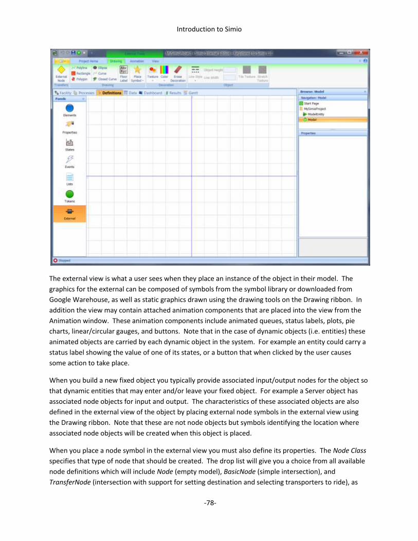
Introduction to Simio
-78-
The external view is what a user sees when they place an instance of the object in their model. The
graphics for the external can be composed of symbols from the symbol library or downloaded from
Google Warehouse, as well as static graphics drawn using the drawing tools on the Drawing ribbon. In
addition the view may contain attached animation components that are placed into the view from the
Animation window. These animation components include animated queues, status labels, plots, pie
charts, linear/circular gauges, and buttons. Note that in the case of dynamic objects (i.e. entities) these
animated objects are carried by each dynamic object in the system. For example an entity could carry a
status label showing the value of one of its states, or a button that when clicked by the user causes
some action to take place.
When you build a new fixed object you typically provide associated input/output nodes for the object so
that dynamic entities that may enter and/or leave your fixed object. For example a Server object has
associated node objects for input and output. The characteristics of these associated objects are also
defined in the external view of the object by placing external node symbols in the external view using
the Drawing ribbon. Note that these are not node objects but symbols identifying the location where
associated node objects will be created when this object is placed.
When you place a node symbol in the external view you must also define its properties. The Node Class
specifies that type of node that should be created. The drop list will give you a choice from all available
node definitions which will include Node (empty model), BasicNode (simple intersection), and
TransferNode (intersection with support for setting destination and selecting transporters to ride), as
Introduction to Simio
-79-
well as any other node definitions that you have loaded as libraries or are defined in your project. In the
case of the Standard Library the BasicNode class is always used for input nodes, and the TransferNode is
used for output nodes. The Input Logic Type specifies how arriving entities attempting to enter this
object are to be handled by this object. The None option specifies that entities are not permitted to
enter. The ProcessStation option specifies that the arriving entity may enter at a specified station, which
fires a station entered event that can be used to trigger process logic. This is used when defining the
object logic using a process model. The FacilityNode option specifies that the arriving entity is to be sent
to a node inside the facility model for the object. This option is used for defining object logic using a
facility model. In the General section the Name for the node symbol is specified. This node symbol
name is used to create the name of the associated node object that is created at this symbol location
when this object is instantiated using the format NodeSymbolName@ObjectName. For example is the
symbol name is Input and the object name is Lathe, the associated object that is automatically created is
named Input@Lathe. In the Standard Library the input node symbols are named Input and output node
symbols are named Output.
Model Logic The logic for a fixed object definition is defined using a facility and/or process model, as determined by
the Input Logic Type on the node symbols. In the case of entities, transporters, nodes and links there
are no node symbols and hence these models are typically built using process logic.
Whenever you have built a model of a system it represents the logic component of an object definition.
You can typically turn any model into a useable object definition by simply adding some properties to
supply inputs to the model, along with an external view to provide a graphical representation for the
object along with nodes that allow entities to enter and exit the model.
There are three approaches to defining the model logic for an object. The first approach is to create
your model hierarchically using a facility model. This approach can also be combined with the use of
add-on processes to define custom behavior within the facility objects. This approach is typically used
for building up higher level facility components such a workcenter comprised of two machines, a
worker, and tooling. The second and most flexible approach is to create the object definition behavior
from scratch using a process model. This is the approach that was used to create the Standard Library.
The third approach is to sub-class an existing object definition and then change/extend its behavior
using processes. This approach is typically used when there is an existing object that has behavior
similar to the desired object, and can be “tweaked” in terms of property names, descriptions, and
behavior to meet the needs of the new object.
The concept of sub-classing an object definition is analogous to the concept of sub-classing objects in a
programming language. The basic idea is that the new object definition that you are building inherits its
properties, states, events, and logic from an existing object definition. The sub-classed object will
initially have the same properties and behavior of the original object, and if the original object definition
is updated, then the sub-classed object will inherit the new behavior. However after sub-classing you
can then hide or rename the inherited properties, selectively override portions of the process logic that
is inherited, or add additional processes to extend the behavior. For example you might create a new
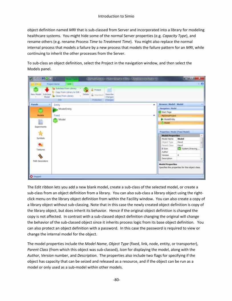
Introduction to Simio
-80-
object definition named MRI that is sub-classed from Server and incorporated into a library for modeling
healthcare systems. You might hide some of the normal Server properties (e.g. Capacity Type), and
rename others (e.g. rename Process Time to Treatment Time). You might also replace the normal
internal process that models a failure by a new process that models the failure pattern for an MRI, while
continuing to inherit the other processes from the Server.
To sub-class an object definition, select the Project in the navigation window, and then select the
Models panel.
The Edit ribbon lets you add a new blank model, create a sub-class of the selected model, or create a
sub-class from an object definition from a library. You can also sub-class a library object using the right-
click menu on the library object definition from within the Facility window. You can also create a copy of
a library object without sub-classing. Note that in this case the newly created object definition is copy of
the library object, but does inherit its behavior. Hence if the original object definition is changed the
copy is not affected. In contrast with a sub-classed object definition changing the original will change
the behavior of the sub-classed object since it inherits process logic from its base object definition. You
can also protect an object definition with a password. In this case the password is required to view or
change the internal model for the object.
The model properties include the Model Name, Object Type (fixed, link, node, entity, or transporter),
Parent Class (from which this object was sub-classed), Icon for displaying the model, along with the
Author, Version number, and Description. The properties also include two flags for specifying if the
object has capacity that can be seized and released as a resource, and if the object can be run as a
model or only used as a sub-model within other models.

Introduction to Simio
-81-
Properties, States, and Events Whenever you create an object definition you inherit properties, states, and events from the base
object class and you can add new members as well. You can view the inherited properties, states, and
events in the Definitions window for the model. The inherited and new members are placed in separate
categories that can be independently expanded and collapsed. The following shows the Properties
panel for a model type Fixed with a single new property named ReworkTime. Note that this property
can be referenced by both the objects and process flows within the model.
The characteristics of ReworkTime are shown in the Property window, and include the Default Value,
Unit Type/Default Units, Display Name, Description, Category Name, and flags specifying if this is a
Required Value and if this property is Visible to the user. The characteristics also include a Switch
Property Name, Switch Condition, and Switch Value. These can be used to hide or show a property
based on the value the user specifies for another property. For example you might have property Y
show only if the user sets property X to value greater than 0. This lets you dynamically configure the
Property window based on user inputs.
In the case of an inherited property you can change the Visible flag along with the Default Value, Display
Name, Description, and Category. Hence you can hide properties or change their general appearance.
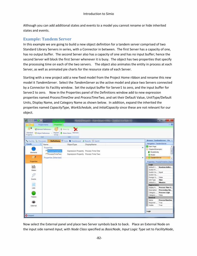
Introduction to Simio
-82-
Although you can add additional states and events to a model you cannot rename or hide inherited
states and events.
Example: Tandem Server In this example we are going to build a new object definition for a tandem server comprised of two
Standard Library Servers in series, with a Connector in between. The first Server has a capacity of one,
has no output buffer. The second Server also has a capacity of one and has no input buffer; hence the
second Server will block the first Server whenever it is busy. The object has two properties that specify
the processing time on each of the two servers. The object also animates the entity in process at each
Server, as well as animated pie charts for the resource state of each Server.
Starting with a new project add a new fixed model from the Project Home ribbon and rename this new
model it TandemServer. Select the TandemServer as the active model and place two Servers connected
by a Connector its Facility window. Set the output buffer for Server1 to zero, and the input buffer for
Server2 to zero. Now in the Properties panel of the Definitions window add to new expression
properties named ProcessTimeOne and ProcessTimeTwo, and set their Default Value, UnitType/Default
Units, Display Name, and Category Name as shown below. In addition, expand the inherited the
properties named CapacityType, WorkSchedule, and IntialCapacity since these are not relevant for our
object.
Now select the External panel and place two Server symbols back to back. Place an External Node on
the input side named Input, with Node Class specified as BasicNode, Input Logic Type set to FacilityNode,

Introduction to Simio
-83-
and Node specified as Input@Server1. Place a second External Node on the output side named Output,
with Node Class specified as TransferNode, and Input Logic Type set to None (no entry allowed on this
side of the tandem server). Using the Animation ribbon draw animated queues for the input buffer, the
two processing stations, and output buffer, and specify the Queue State as
Server1.InputBuffer.Contents, Server1.Processing.Contents, Server2.Processing.Contents, and
Server2.OutputBuffer.Contents. Also add to animated pie charts specifying the Data Type as ListState
and List State as Server1.ResourceState and Server2.ResourceState, respectively, as shown below:
Note that in our external view we are sending entities arriving to the associated node that is created by
the Input node symbol to the node named Input@Server1 in our facility model of the TandemServer.
Here they will proceed through the two Servers until they reach the output node of Server2, where we
want to send them back up to the associated node defined by the external node symbol named Output.
To do this return to the facility model for TandemServer and click on the output node for Server2 and
under the General category set the AutoTransferOnExit flag to True and specify the External Node Name
as Output. This will cause the departing entities to be sent out from the associated output node that is
created for the Output symbol.
We will also edit the processing time for Server1 to be ProcessTimeOne and the processing time for
Server2 to be ProcessTimeTwo. Hence these processing times are specified by our newly created
properties for TandemServer.
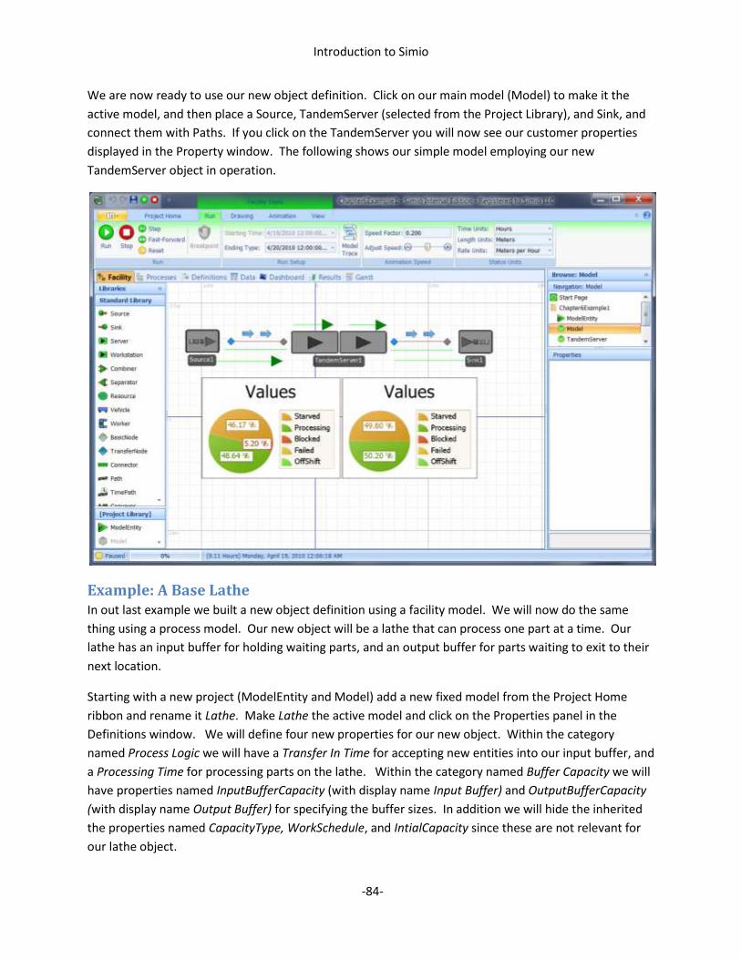
Introduction to Simio
-84-
We are now ready to use our new object definition. Click on our main model (Model) to make it the
active model, and then place a Source, TandemServer (selected from the Project Library), and Sink, and
connect them with Paths. If you click on the TandemServer you will now see our customer properties
displayed in the Property window. The following shows our simple model employing our new
TandemServer object in operation.
Example: A Base Lathe In out last example we built a new object definition using a facility model. We will now do the same
thing using a process model. Our new object will be a lathe that can process one part at a time. Our
lathe has an input buffer for holding waiting parts, and an output buffer for parts waiting to exit to their
next location.
Starting with a new project (ModelEntity and Model) add a new fixed model from the Project Home
ribbon and rename it Lathe. Make Lathe the active model and click on the Properties panel in the
Definitions window. We will define four new properties for our new object. Within the category
named Process Logic we will have a Transfer In Time for accepting new entities into our input buffer, and
a Processing Time for processing parts on the lathe. Within the category named Buffer Capacity we will
have properties named InputBufferCapacity (with display name Input Buffer) and OutputBufferCapacity
(with display name Output Buffer) for specifying the buffer sizes. In addition we will hide the inherited
the properties named CapacityType, WorkSchedule, and IntialCapacity since these are not relevant for
our lathe object.
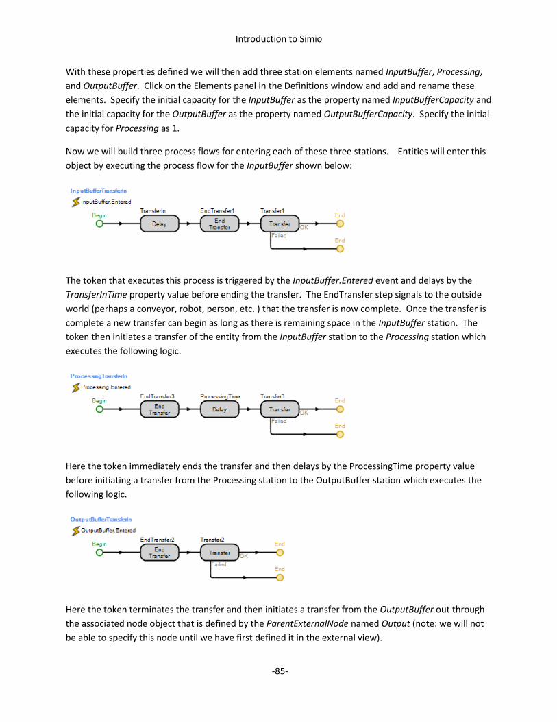
Introduction to Simio
-85-
With these properties defined we will then add three station elements named InputBuffer, Processing,
and OutputBuffer. Click on the Elements panel in the Definitions window and add and rename these
elements. Specify the initial capacity for the InputBuffer as the property named InputBufferCapacity and
the initial capacity for the OutputBuffer as the property named OutputBufferCapacity. Specify the initial
capacity for Processing as 1.
Now we will build three process flows for entering each of these three stations. Entities will enter this
object by executing the process flow for the InputBuffer shown below:
The token that executes this process is triggered by the InputBuffer.Entered event and delays by the
TransferInTime property value before ending the transfer. The EndTransfer step signals to the outside
world (perhaps a conveyor, robot, person, etc. ) that the transfer is now complete. Once the transfer is
complete a new transfer can begin as long as there is remaining space in the InputBuffer station. The
token then initiates a transfer of the entity from the InputBuffer station to the Processing station which
executes the following logic.
Here the token immediately ends the transfer and then delays by the ProcessingTime property value
before initiating a transfer from the Processing station to the OutputBuffer station which executes the
following logic.
Here the token terminates the transfer and then initiates a transfer from the OutputBuffer out through
the associated node object that is defined by the ParentExternalNode named Output (note: we will not
be able to specify this node until we have first defined it in the external view).

Introduction to Simio
-86-
Next we will define the external view. Click on the External panel in the Definitions window and place a
lathe symbol from the symbol library in the center of the external view, and add an external node with
Class Type BasicNode and named Input on the left side of the lathe, and an external node with Class
Type TransferNode and named Output on the right side of the lathe (we can now go back and specify our
ParentExternalNode named Output on our OutputBuffer Transfer step). Specify the Input Logic Type on
the Input external node as ProcessStation, and then select InputBuffer from the drop list. Note that
arriving entities will transfer to the InputBuffer station upon arrival to the associated node object
corresponding to this external node symbol. We will add animated queues for animating the
InputBuffer, Processing, and OutputBuffer stations. Our external view for the Lathe is shown below:
We are now ready to use our new object definition in a model. Click on Model in the navigation window
to make it our active model and drag out a Source, Lathe (from the Project Library), and Sink, and
connect them with Paths. Click on Lathe to edit its properties. You can now run the model.
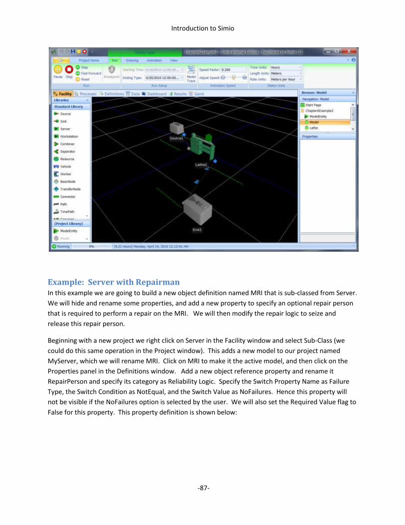
Introduction to Simio
-87-
Example: Server with Repairman In this example we are going to build a new object definition named MRI that is sub-classed from Server.
We will hide and rename some properties, and add a new property to specify an optional repair person
that is required to perform a repair on the MRI. We will then modify the repair logic to seize and
release this repair person.
Beginning with a new project we right click on Server in the Facility window and select Sub-Class (we
could do this same operation in the Project window). This adds a new model to our project named
MyServer, which we will rename MRI. Click on MRI to make it the active model, and then click on the
Properties panel in the Definitions window. Add a new object reference property and rename it
RepairPerson and specify its category as Reliability Logic. Specify the Switch Property Name as Failure
Type, the Switch Condition as NotEqual, and the Switch Value as NoFailures. Hence this property will
not be visible if the NoFailures option is selected by the user. We will also set the Required Value flag to
False for this property. This property definition is shown below:

Introduction to Simio
-88-
We will also hide the inherited properties named Capacity Type, WorkSchedule, and InitialCapacity, and
rename the ProcessingTime property to Treatment Time, and enter a new description for this property.
Next we will define the external view for the MRI. Click on the External panel in the Definitions window,
and then in the Place Symbol drop list select Download Symbol to download an MRI graphic from
Google Warehouse and add animated queues for the queue states InputBuffer.Contents,
Processing.Contents, and OutputBuffer.Contents. Note that the two external node symbols are
inherited from the Server and cannot be modified.
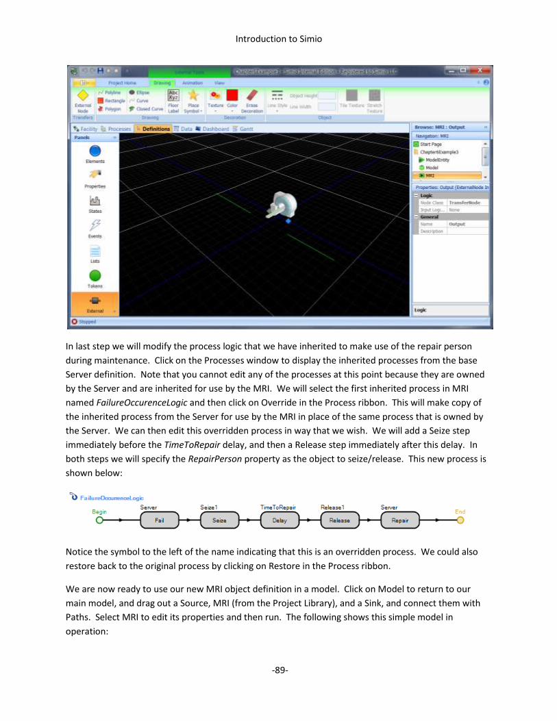
Introduction to Simio
-89-
In last step we will modify the process logic that we have inherited to make use of the repair person
during maintenance. Click on the Processes window to display the inherited processes from the base
Server definition. Note that you cannot edit any of the processes at this point because they are owned
by the Server and are inherited for use by the MRI. We will select the first inherited process in MRI
named FailureOccurenceLogic and then click on Override in the Process ribbon. This will make copy of
the inherited process from the Server for use by the MRI in place of the same process that is owned by
the Server. We can then edit this overridden process in way that we wish. We will add a Seize step
immediately before the TimeToRepair delay, and then a Release step immediately after this delay. In
both steps we will specify the RepairPerson property as the object to seize/release. This new process is
shown below:
Notice the symbol to the left of the name indicating that this is an overridden process. We could also
restore back to the original process by clicking on Restore in the Process ribbon.
We are now ready to use our new MRI object definition in a model. Click on Model to return to our
main model, and drag out a Source, MRI (from the Project Library), and a Sink, and connect them with
Paths. Select MRI to edit its properties and then run. The following shows this simple model in
operation:

Introduction to Simio
-90-
Summary In this chapter we have reviewed the basic concepts for building object definitions in Simio. This is a key
feature of Simio because it allows non-programmers to build custom objects that are focused on a
specific model or application area.
In our examples here we placed our objects from the Project Library. The other alternative is to build
the object definitions in their own project and then load that project as a library from the Project Home
ribbon.
With Simio you often have the choice to make between working with the Standard Library embellished
with add-on processes, and creating a new library with custom logic. If you encounter the same
applications over and over again it is more convenient to build custom objects and thereby avoid the
repeated need for add-on processes. Of course you can also provide support for add-on processes in
your own objects by simply defining a property for the process name and passing that property to an
Execute step within your process.
With a bit of experience you will find object building to be a simple and powerful capability for your
modeling activities.
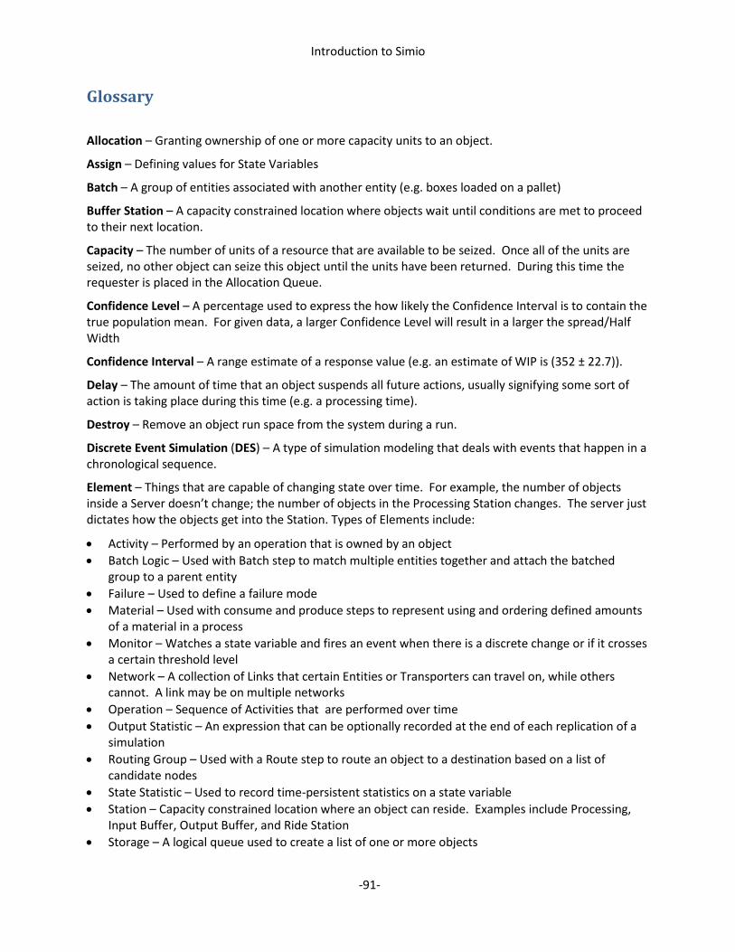
Introduction to Simio
-91-
Glossary
Allocation – Granting ownership of one or more capacity units to an object.
Assign – Defining values for State Variables
Batch – A group of entities associated with another entity (e.g. boxes loaded on a pallet)
Buffer Station – A capacity constrained location where objects wait until conditions are met to proceed to their next location.
Capacity – The number of units of a resource that are available to be seized. Once all of the units are seized, no other object can seize this object until the units have been returned. During this time the requester is placed in the Allocation Queue.
Confidence Level – A percentage used to express the how likely the Confidence Interval is to contain the true population mean. For given data, a larger Confidence Level will result in a larger the spread/Half Width
Confidence Interval – A range estimate of a response value (e.g. an estimate of WIP is (352 ± 22.7)).
Delay – The amount of time that an object suspends all future actions, usually signifying some sort of action is taking place during this time (e.g. a processing time).
Destroy – Remove an object run space from the system during a run.
Discrete Event Simulation (DES) – A type of simulation modeling that deals with events that happen in a chronological sequence.
Element – Things that are capable of changing state over time. For example, the number of objects inside a Server doesn’t change; the number of objects in the Processing Station changes. The server just dictates how the objects get into the Station. Types of Elements include:
Activity – Performed by an operation that is owned by an object
Batch Logic – Used with Batch step to match multiple entities together and attach the batched group to a parent entity
Failure – Used to define a failure mode
Material – Used with consume and produce steps to represent using and ordering defined amounts of a material in a process
Monitor – Watches a state variable and fires an event when there is a discrete change or if it crosses a certain threshold level
Network – A collection of Links that certain Entities or Transporters can travel on, while others cannot. A link may be on multiple networks
Operation – Sequence of Activities that are performed over time
Output Statistic – An expression that can be optionally recorded at the end of each replication of a simulation
Routing Group – Used with a Route step to route an object to a destination based on a list of candidate nodes
State Statistic – Used to record time-persistent statistics on a state variable
Station – Capacity constrained location where an object can reside. Examples include Processing, Input Buffer, Output Buffer, and Ride Station
Storage – A logical queue used to create a list of one or more objects
Introduction to Simio
-92-
Tally Statistic – Tallies observational statistics that are recorded using a Tally Step
Timer – Fires a stream of events according to a specified interval type
Entity – Part of an object model and can have its own intelligent behavior. They can make decisions, reject requests, decide to take a rest, etc. Entities have object definitions just like the other objects in the model. Entity objects can be dynamically created and destroyed, moved across a network of Links and Nodes, move through 3D space, and move into and out of Fixed objects. Examples of Entity objects include customers, parts or work pieces.
Event – A notification that can be given by one object and responded to by several. It alerts other objects that an action has occurred.
Experiment – Part of the project that is used for output analysis. The user defines one or more sets of inputs/outputs (Scenarios) and runs multiple replications to get statistically valid results from which to draw conclusions.
Half Width – Half of the confidence interval. CI = Average ± Half Width. The smaller the Half Width the smaller the variability.
Library – A collection of objects/models that can be used to create a model.
Link – Pathways for entity/transporter movement. There are four types of links:
Connector – Used to define a non-passing pathway between two node locations where travel time is instantaneous. Entities will never actually enter, move across or exit a connector, but will always instead immediately do a node-to-node direct transfer.
Conveyor – Represents either accumulating or non-accumulating conveyors and supports both fixed and variable spacing.
Path – Used to define a pathway between two node locations where the travel time is determined by the path length and a traveler’s speed.
Time Path – Used to define a pathway between two node locations where the travel time is user specified.
Member – The object owned by the Parent
Model – A representation of real world object or collection of objects that interact with each other. Models are usually used to make decisions and are defined by their properties, states, events, external view, and logic.
Network – A collection of Links that certain Entities or Transporters can travel on, while others cannot. A link may be on multiple networks
Object Hierarchy:
Object Definition – A collection of Properties, States, Events, Elements, and other characteristics that defines the logic and behavior of an object and how it interacts with other objects. Every model is an object definition that can be potentially used in another model.
Object Instance – An object definition that is placed into Simio’s Facility View. It carries unique property values to identify it and customize its behavior (e.g. an entity’s target speed).
Object Run Space – Objects that are created during a run that carry with them states to record system changes (e.g. an entity’s current speed). These object run spaces refer back to the object instance for their properties and to the object definition for their logic and behavior.
Parent – The “owner” of another object
Introduction to Simio
-93-
Passing – Allowing one object to travel through another object on a link.
Priority – Numeric property for all Entities used to make Ranking Rules or Dynamic Selection Rules to order how entities are to be moved throughout a model.
Process – A sequence of commands that dictate the behavior of an object. Specified graphically by placing Steps in a flow process diagram.
Project – A collection of Models and Experiments that are used to represent a system.
Property – Input parameters that are associated with the object that define exactly how the object interacts with other objects. Ex – Processing Time, Selection Rule, Priority, Transfer-In Time
PseudoRandom – something that appears to be random, but is not. DES random number generators are PseudoRandom in that they have predictability. It repeats the same random number stream every time you press “Run” and can be used again and again, useful for testing and fixing models
Queue – A collection of objects waiting for an event to occur that will allow them to enter a station, seize an object, enter a link, etc.
Release – Freeing one or more units of the reserved object to allow seizing by other objects.
Replication – Running a scenario one time, usually run multiple replications per scenario. The more replications the more accurate the statistics.
Resource – An object that represents a system constraint and can be seized and released. Any object can be a resource. Resources may be given intelligent behavior and interaction with other objects.
Scenario – A set of input values to be run in an experiment, usually a possible future state of the system being evaluated.
Selection Weight – Property of all links that determines the likelihood of choosing that particular link as an outbound link from an object. Maybe be a simple number or a complex expression.
Seize – To reserve one or more units of an object for use by the requesting object. While an object is seized no other object can take possession of that object.
Server – An object that consists of three stations: Input Buffer, Processing, and Output Buffer. Usually represents a location that has a capacitated process.
State – Dynamic values that may change as the model executes. There are four types of states:
Discrete State – represents a numeric value that may change instantaneously at discrete event times
Level State – represents a variable that has a numeric value that may change continuously over time based on the value of the rate.
List State – represents an integer value corresponding to one of several entries from a string list.
Movement State – represents a variable that has a numeric value that may change continuously over time based on the current value of the rate and acceleration.
Step – Used to define logic within a process. Each step performs an action (such as seize, delay, decide, or wait).
Stochastic Process – A process whose behavior is non-deterministic, meaning that there is randomness in the process.
Token – Executes the steps in a process flow. A Token may have one or more user defined states that carry information from step to step.

Introduction to Simio
-94-
Transporter – A transporter object is a special type of entity that can pickup entity objects at a location, carry those entities through a network of links or free space, and then drop the entities off at a destination.
Validation – Determining if the model is an accurate representation of the real system – if the model’s output matches the real system sufficiently to meet the model objectives.
Variability – A measure of how spread the observed data values are. A key cause of variability is the randomness incorporated into typical simulation models.
Vehicle – A transporter object that represents a machine. A vehicle has the possibility of failures representing breakdowns.
Verification – Determining if the model is built correctly - i.e. with the correct input logic, parameters, and values
Worker – A transporter object that represents a human. A worker has the ability to follow a work schedule.

Introduction to Simio
-95-
Technical Support and Resources
Technical Support The best way to get support is to contact us on-line at Simio Support.
(http://simio.devsuite.net/scripts/texcel/CustomerWise/CLogin.dll?ProjectID=20)
You will be able to immediately search the knowledgebase for common problems and commonly
requested information. In addition, registered users can submit and track support requests (incidents)
and suggestions for enhancements.
You can also email our support staff using [email protected] or call us at +1-412-528-1576 or toll free
at 1-877-297-4646.
You will need to know your Simio Version Number which can be found on the lower right corner of the
Simio start page. Although the complete number is 12 digits long (x.xx.xxxx.xxxxx), you will generally
only need the first 3 digits, for example 2.39.
Simio User’s Forum You will find the Simio User’s Forum at http://www.simio.com/forums. Here you will find more product
information, a place to post questions, and the opportunity to engage in discussions with other users
and the Simio team.
We encourage you to also join the Simio Insiders group. This has been established to let you become an
important part of our process; essentially an extension to our team. Please visit our simulation
community resources web page (http://www.simio.com/community.html) for additional information.
More Information Please consult the Start Page of the software for a description of more available resources and how to
contact us with ideas, questions, or problems.
While Simio includes comprehensive help available at the touch of “F1” in the product, if you prefer a
printable version, you will find a link to the Simio Reference Guide.pdf on the Start Page. And you will
find a link to our increasing number of Training Videos.
Using This Material While this document is protected by copyright, we support and encourage it use in Simio education. For
educational purposes, you are free to reuse this material and excerpts from it in derivative works as long
as the original source is cited.