
Introduction to Robotics...
32
Robotics Probabilities Random variables, joint, conditional, marginal distribution, Bayes theorem, Probability distributions, Gauss, Dirac, Conjugate priors Marc Toussaint University of Stuttgart Winter 2017/18 Lecturer: Duy Nguyen-Tuong Bosch Center for AI - Research Dept.
Transcript of Introduction to Robotics...

Robotics
Probabilities
Random variables, joint, conditional, marginaldistribution, Bayes theorem, Probability
distributions, Gauss, Dirac, Conjugate priors
Marc ToussaintUniversity of Stuttgart
Winter 2017/18
Lecturer: Duy Nguyen-Tuong
Bosch Center for AI - Research Dept.
Probability Theory
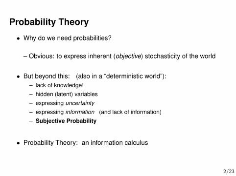
• Why do we need probabilities?
– Obvious: to express inherent (objective) stochasticity of the world
• But beyond this: (also in a “deterministic world”):– lack of knowledge!– hidden (latent) variables– expressing uncertainty– expressing information (and lack of information)– Subjective Probability
• Probability Theory: an information calculus
2/23
Probability Theory
• Why do we need probabilities?
– Obvious: to express inherent (objective) stochasticity of the world
• But beyond this: (also in a “deterministic world”):– lack of knowledge!– hidden (latent) variables– expressing uncertainty– expressing information (and lack of information)– Subjective Probability
• Probability Theory: an information calculus
2/23
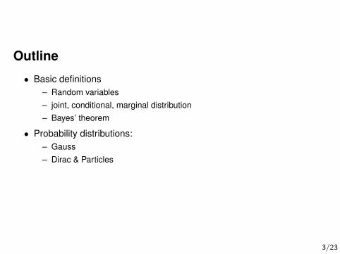
Outline
• Basic definitions– Random variables– joint, conditional, marginal distribution– Bayes’ theorem
• Probability distributions:– Gauss– Dirac & Particles
3/23
Basic definitions
4/23
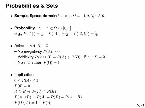
Probabilities & Sets
• Sample Space/domain Ω, e.g. Ω = 1, 2, 3, 4, 5, 6
• Probability P : A ⊂ Ω 7→ [0, 1]
e.g., P (1) = 16 , P (4) = 1
6 , P (2, 5) = 13 ,
• Axioms: ∀A,B ⊆ Ω
– Nonnegativity P (A) ≥ 0
– Additivity P (A ∪B) = P (A) + P (B) if A ∩B = ∅– Normalization P (Ω) = 1
• Implications0 ≤ P (A) ≤ 1
P (∅) = 0
A ⊆ B ⇒ P (A) ≤ P (B)
P (A ∪B) = P (A) + P (B)− P (A ∩B)
P (Ω \A) = 1− P (A)5/23
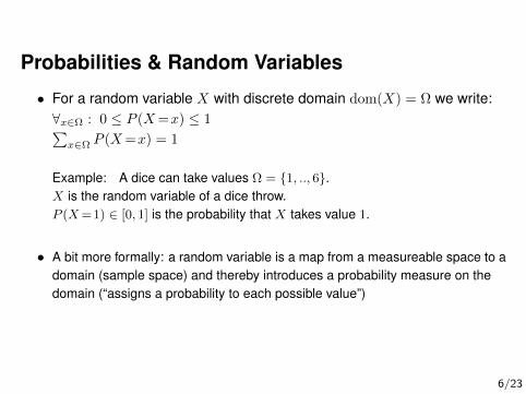
Probabilities & Random Variables
• For a random variable X with discrete domain dom(X) = Ω we write:∀x∈Ω : 0 ≤ P (X=x) ≤ 1∑x∈Ω P (X=x) = 1
Example: A dice can take values Ω = 1, .., 6.X is the random variable of a dice throw.P (X=1) ∈ [0, 1] is the probability that X takes value 1.
• A bit more formally: a random variable is a map from a measureable space to adomain (sample space) and thereby introduces a probability measure on thedomain (“assigns a probability to each possible value”)
6/23
Probabilty Distributions
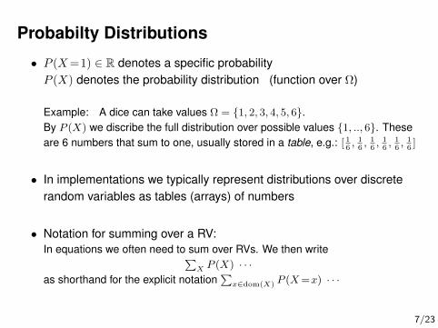
• P (X=1) ∈ R denotes a specific probabilityP (X) denotes the probability distribution (function over Ω)
Example: A dice can take values Ω = 1, 2, 3, 4, 5, 6.By P (X) we discribe the full distribution over possible values 1, .., 6. Theseare 6 numbers that sum to one, usually stored in a table, e.g.: [ 1
6, 16, 16, 16, 16, 16]
• In implementations we typically represent distributions over discreterandom variables as tables (arrays) of numbers
• Notation for summing over a RV:In equations we often need to sum over RVs. We then write∑
X P (X) · · ·as shorthand for the explicit notation
∑x∈dom(X) P (X=x) · · ·
7/23
Probabilty Distributions
• P (X=1) ∈ R denotes a specific probabilityP (X) denotes the probability distribution (function over Ω)
Example: A dice can take values Ω = 1, 2, 3, 4, 5, 6.By P (X) we discribe the full distribution over possible values 1, .., 6. Theseare 6 numbers that sum to one, usually stored in a table, e.g.: [ 1
6, 16, 16, 16, 16, 16]
• In implementations we typically represent distributions over discreterandom variables as tables (arrays) of numbers
• Notation for summing over a RV:In equations we often need to sum over RVs. We then write∑
X P (X) · · ·as shorthand for the explicit notation
∑x∈dom(X) P (X=x) · · ·
7/23
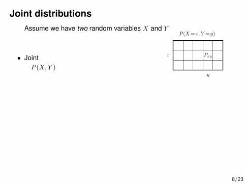
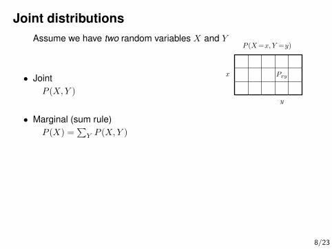
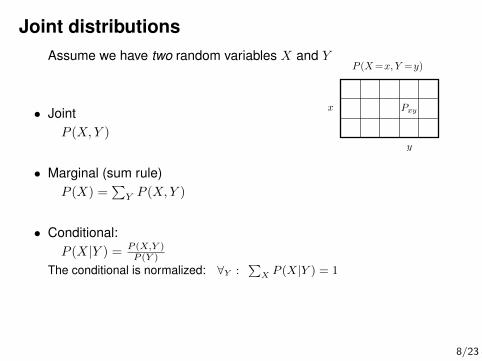
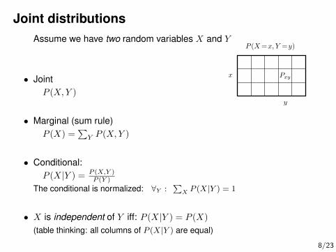
Joint distributionsAssume we have two random variables X and Y
• JointP (X,Y )
• Marginal (sum rule)P (X) =
∑Y P (X,Y )
• Conditional:P (X|Y ) = P (X,Y )
P (Y )
The conditional is normalized: ∀Y :∑
X P (X|Y ) = 1
• X is independent of Y iff: P (X|Y ) = P (X)
(table thinking: all columns of P (X|Y ) are equal)
8/23
Bayes’ Theorem
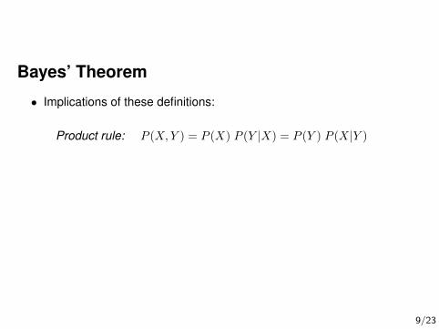
• Implications of these definitions:
Product rule: P (X,Y ) = P (X) P (Y |X) = P (Y ) P (X|Y )
Bayes’ Theorem: P (X|Y ) = P (Y |X) P (X)P (Y )
posterior = likelihood · priornormalization
9/23
Bayes’ Theorem
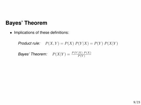
• Implications of these definitions:
Product rule: P (X,Y ) = P (X) P (Y |X) = P (Y ) P (X|Y )
Bayes’ Theorem: P (X|Y ) = P (Y |X) P (X)P (Y )
posterior = likelihood · priornormalization
9/23
Bayes’ Theorem
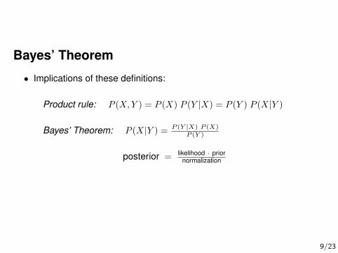
• Implications of these definitions:
Product rule: P (X,Y ) = P (X) P (Y |X) = P (Y ) P (X|Y )
Bayes’ Theorem: P (X|Y ) = P (Y |X) P (X)P (Y )
posterior = likelihood · priornormalization
9/23
Multiple RVs:
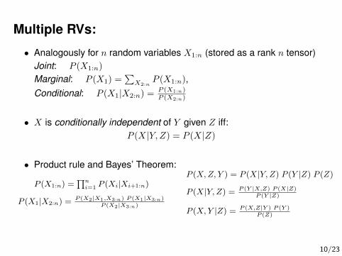
• Analogously for n random variables X1:n (stored as a rank n tensor)Joint: P (X1:n)
Marginal: P (X1) =∑X2:n
P (X1:n),Conditional: P (X1|X2:n) = P (X1:n)
P (X2:n)
• X is conditionally independent of Y given Z iff:P (X|Y,Z) = P (X|Z)
• Product rule and Bayes’ Theorem:
P (X1:n) =∏n
i=1 P (Xi|Xi+1:n)
P (X1|X2:n) = P (X2|X1,X3:n) P (X1|X3:n)P (X2|X3:n)
P (X,Z, Y ) = P (X|Y,Z) P (Y |Z) P (Z)
P (X|Y,Z) = P (Y |X,Z) P (X|Z)P (Y |Z)
P (X,Y |Z) = P (X,Z|Y ) P (Y )P (Z)
10/23
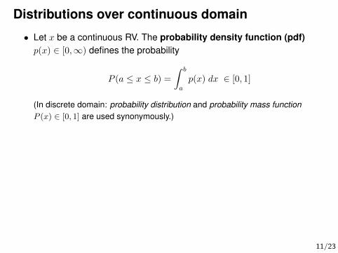
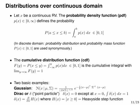
Distributions over continuous domain
• Let x be a continuous RV. The probability density function (pdf)p(x) ∈ [0,∞) defines the probability
P (a ≤ x ≤ b) =
∫ b
a
p(x) dx ∈ [0, 1]
(In discrete domain: probability distribution and probability mass functionP (x) ∈ [0, 1] are used synonymously.)
• The cumulative distribution function (cdf)F (y) = P (x ≤ y) =
∫ y−∞ p(x)dx ∈ [0, 1] is the cumulative integral with
limy→∞ F (y) = 1
• Two basic examples:Gaussian: N(x |µ,Σ) = 1
| 2πΣ | 1/2 e− 1
2 (x−µ)> Σ-1 (x−µ)
Dirac or δ (“point particle”) δ(x) = 0 except at x = 0,∫δ(x) dx = 1
δ(x) = ∂∂xH(x) where H(x) = [x ≥ 0] = Heavyside step function
11/23
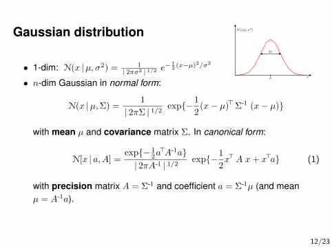
Gaussian distribution
• 1-dim: N(x |µ, σ2) = 1| 2πσ2 | 1/2 e
− 12 (x−µ)2/σ2
N (x|µ, σ2)
x
2σ
µ
• n-dim Gaussian in normal form:
N(x |µ,Σ) =1
| 2πΣ | 1/2exp−1
2(x− µ)>Σ-1 (x− µ)
with mean µ and covariance matrix Σ. In canonical form:
N[x | a,A] =exp− 1
2a>A-1a
| 2πA-1 | 1/2exp−1
2x>A x+ x>a (1)
with precision matrix A = Σ-1 and coefficient a = Σ-1µ (and meanµ = A-1a).
12/23
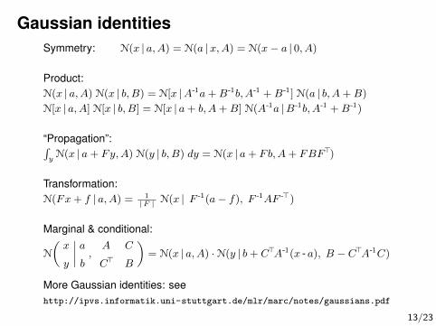
Gaussian identitiesSymmetry: N(x | a,A) = N(a |x,A) = N(x− a | 0, A)
Product:N(x | a,A) N(x | b,B) = N[x |A-1a + B-1b, A-1 + B-1] N(a | b, A + B)
N[x | a,A] N[x | b,B] = N[x | a + b, A + B] N(A-1a |B-1b, A-1 + B-1)
“Propagation”:∫yN(x | a + Fy,A) N(y | b,B) dy = N(x | a + Fb,A + FBF>)
Transformation:N(Fx + f | a,A) = 1
|F | N(x | F -1(a− f), F -1AF ->)
Marginal & conditional:
N
(x
y
∣∣∣∣ ab,
A C
C> B
)= N(x | a,A) ·N(y | b + C>A-1(x - a), B − C>A-1C)
More Gaussian identities: seehttp://ipvs.informatik.uni-stuttgart.de/mlr/marc/notes/gaussians.pdf
13/23
Motivation for Gaussian distributions
• Gaussian Bandits
• Control theory, Stochastic Optimal Control
• State estimation, sensor processing, Gaussian filtering (Kalmanfiltering)
• Machine Learning
• rich vocabulary and easy to compute!
• etc.
14/23
Dirac Delta / Point ParticleDirac or δ (“point particle”): δ(x) = 0 except at x = 0,
∫δ(x) dx = 1
δ(x) = ∂∂xH(x) where H(x) = [x ≥ 0] is the Heavyside step function
15/23
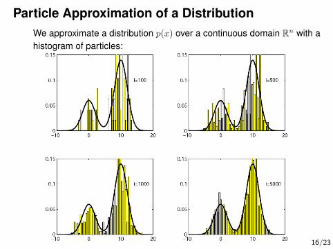
Particle Approximation of a DistributionWe approximate a distribution p(x) over a continuous domain Rn with ahistogram of particles:
16/23
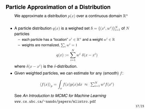
Particle Approximation of a DistributionWe approximate a distribution p(x) over a continuous domain Rn
• A particle distribution q(x) is a weighed set S = (xi, wi)Ni=1 of Nparticles
– each particle has a “location” xi ∈ Rn and a weight wi ∈ R– weights are normalized,
∑i w
i = 1
q(x) :=
N∑i=1
wi δ(x− xi)
where δ(x− xi) is the δ-distribution.
• Given weighted particles, we can estimate for any (smooth) f :
〈f(x)〉p =
∫x
f(x)p(x)dx ≈∑Ni=1 w
if(xi)
See An Introduction to MCMC for Machine Learningwww.cs.ubc.ca/~nando/papers/mlintro.pdf
17/23
Motivation for particle distributions
• Numeric representation of “difficult” distributions– Very general and versatile– But often needs many samples
• Distributions over games (action sequences), sample based planning,MCTS
• State estimation, particle filters
• etc.
18/23
Conjugate priors
• Assume you have data D = x1, .., xn with likelihood
P (D | θ)
that depends on an uncertain parameter θAssume you have a prior P (θ)
• The prior P (θ) is conjugate to the likelihood P (D | θ) iff the posterior
P (θ |D) ∝ P (D | θ) P (θ)
is in the same distribution class as the prior P (θ)
• Having a conjugate prior is very convenient, because then you knowhow to update the belief given data
19/23
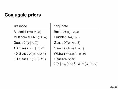
Conjugate priors
likelihood conjugate
Binomial Bin(D |µ) Beta Beta(µ | a, b)Multinomial Mult(D |µ) Dirichlet Dir(µ |α)
Gauss N(x |µ,Σ) Gauss N(µ |µ0, A)
1D Gauss N(x |µ, λ-1) Gamma Gam(λ | a, b)nD Gauss N(x |µ,Λ-1) Wishart Wish(Λ |W, ν)
nD Gauss N(x |µ,Λ-1) Gauss-WishartN(µ |µ0, (βΛ)-1) Wish(Λ |W, ν)
20/23
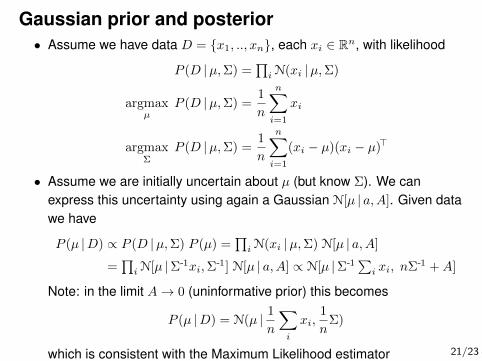
Gaussian prior and posterior• Assume we have data D = x1, .., xn, each xi ∈ Rn, with likelihood
P (D |µ,Σ) =∏iN(xi |µ,Σ)
argmaxµ
P (D |µ,Σ) =1
n
n∑i=1
xi
argmaxΣ
P (D |µ,Σ) =1
n
n∑i=1
(xi − µ)(xi − µ)>
• Assume we are initially uncertain about µ (but know Σ). We canexpress this uncertainty using again a Gaussian N[µ | a,A]. Given datawe have
P (µ |D) ∝ P (D |µ,Σ) P (µ) =∏iN(xi |µ,Σ) N[µ | a,A]
=∏iN[µ |Σ-1xi,Σ
-1] N[µ | a,A] ∝ N[µ |Σ-1∑i xi, nΣ-1 +A]
Note: in the limit A→ 0 (uninformative prior) this becomes
P (µ |D) = N(µ | 1
n
∑i
xi,1
nΣ)
which is consistent with the Maximum Likelihood estimator 21/23
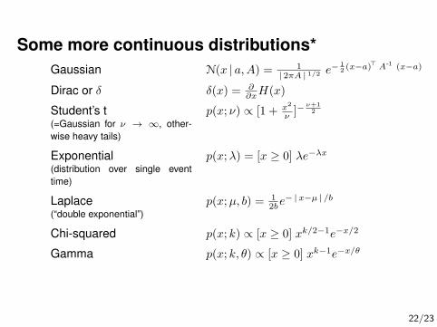
Some more continuous distributions*Gaussian N(x | a,A) = 1
| 2πA | 1/2 e− 1
2 (x−a)> A-1 (x−a)
Dirac or δ δ(x) = ∂∂xH(x)
Student’s t(=Gaussian for ν → ∞, other-wise heavy tails)
p(x; ν) ∝ [1 + x2
ν ]−ν+12
Exponential(distribution over single eventtime)
p(x;λ) = [x ≥ 0] λe−λx
Laplace(“double exponential”)
p(x;µ, b) = 12be− | x−µ | /b
Chi-squared p(x; k) ∝ [x ≥ 0] xk/2−1e−x/2
Gamma p(x; k, θ) ∝ [x ≥ 0] xk−1e−x/θ
22/23
Probability distributions
Bishop, C. M.: Pattern Recognitionand Machine Learning.Springer, 2006http://research.microsoft.com/
en-us/um/people/cmbishop/prml/
23/23