Introduction to Radar Systems - TU · PDF fileIntroduction to Radar Systems Simon Wagner...
30
© Fraunhofer FHR Introduction to Radar Systems Simon Wagner Fraunhofer FHR Cognitive Radar Department CoSIP Workshop Berlin, 07.12.2016
Transcript of Introduction to Radar Systems - TU · PDF fileIntroduction to Radar Systems Simon Wagner...

© Fraunhofer FHR
Introduction to Radar Systems
Simon Wagner
Fraunhofer FHR
Cognitive Radar Department
CoSIP Workshop
Berlin, 07.12.2016
© Fraunhofer FHR
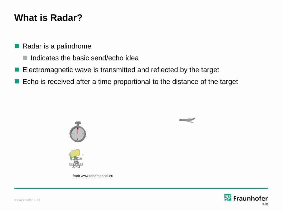
What is Radar?
Radar is a palindrome
Indicates the basic send/echo idea
Electromagnetic wave is transmitted and reflected by the target
Echo is received after a time proportional to the distance of the target
from www.radartutorial.eu
© Fraunhofer FHR
Is an active system (apart from passive radars)
A microwave radiation is emitted by the radar. The reflected radiation,
known as the echo, is backscattered from the surface and received some
time later.
Passive radars use foreign sources of illumination (e.g. FM radio, DVB-T,
foreign remote sensing satellites …)
Independent on the day light, operation at day and night
Operates at microwave frequencies
Usual wavelength between 10 m – 0.1 mm
Clouds, fog, smoke, dust and other materials can be penetrated
RADIO DETECTION AND RANGING (RADAR)
© Fraunhofer FHR
RADAR
Two basic concepts
Radar sensor for object detection
and positioning
Position measurements over time
allow target tracking
The resolution cells (range,
direction, Doppler) are greater or
equal to the object dimensions
Classification by signal strength
(RCS), Doppler modulation,
polarisation, dynamics of motion…
Imaging radar
Generation of a quasi optical image
(SAR, ISAR)
Resolution cells much smaller than
target dimension
Classification with range profiles,
radar images
© Fraunhofer FHR
Radar Transmitter and Receiver
(and other wireless transmission systems)
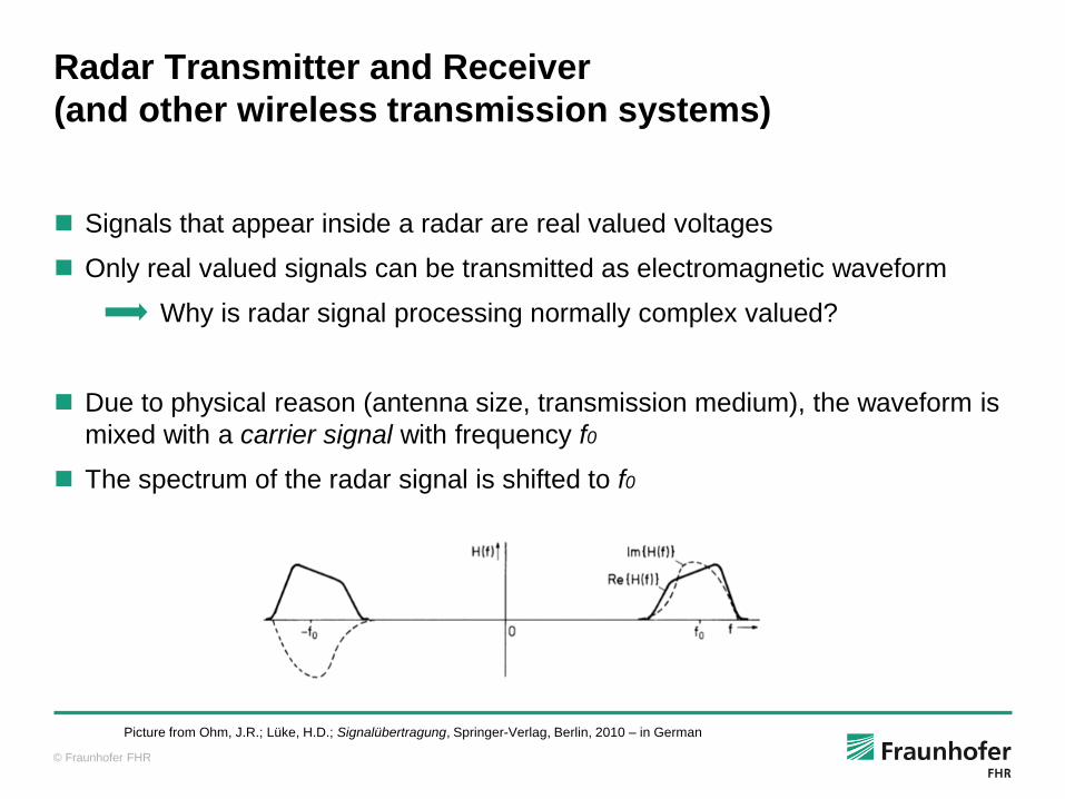
Signals that appear inside a radar are real valued voltages
Only real valued signals can be transmitted as electromagnetic waveform
Why is radar signal processing normally complex valued?
Due to physical reason (antenna size, transmission medium), the waveform is
mixed with a carrier signal with frequency f0
The spectrum of the radar signal is shifted to f0
Picture from Ohm, J.R.; Lüke, H.D.; Signalübertragung, Springer-Verlag, Berlin, 2010 – in German
© Fraunhofer FHR
Radar Transmitter and Receiver
(and other wireless transmission systems)
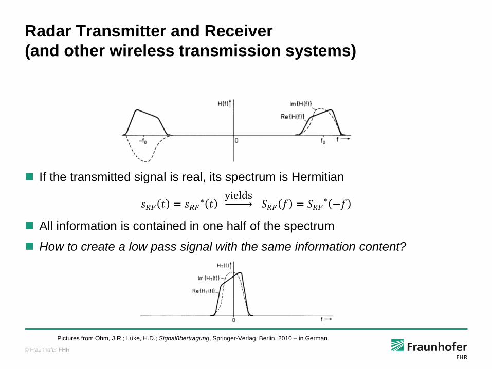
If the transmitted signal is real, its spectrum is Hermitian
𝑠𝑅𝐹 𝑡 = 𝑠𝑅𝐹∗ 𝑡
yields 𝑆𝑅𝐹 𝑓 = 𝑆𝑅𝐹
∗ −𝑓
All information is contained in one half of the spectrum
How to create a low pass signal with the same information content?
Pictures from Ohm, J.R.; Lüke, H.D.; Signalübertragung, Springer-Verlag, Berlin, 2010 – in German
© Fraunhofer FHR
Radar Transmitter and Receiver
(and other wireless transmission systems)
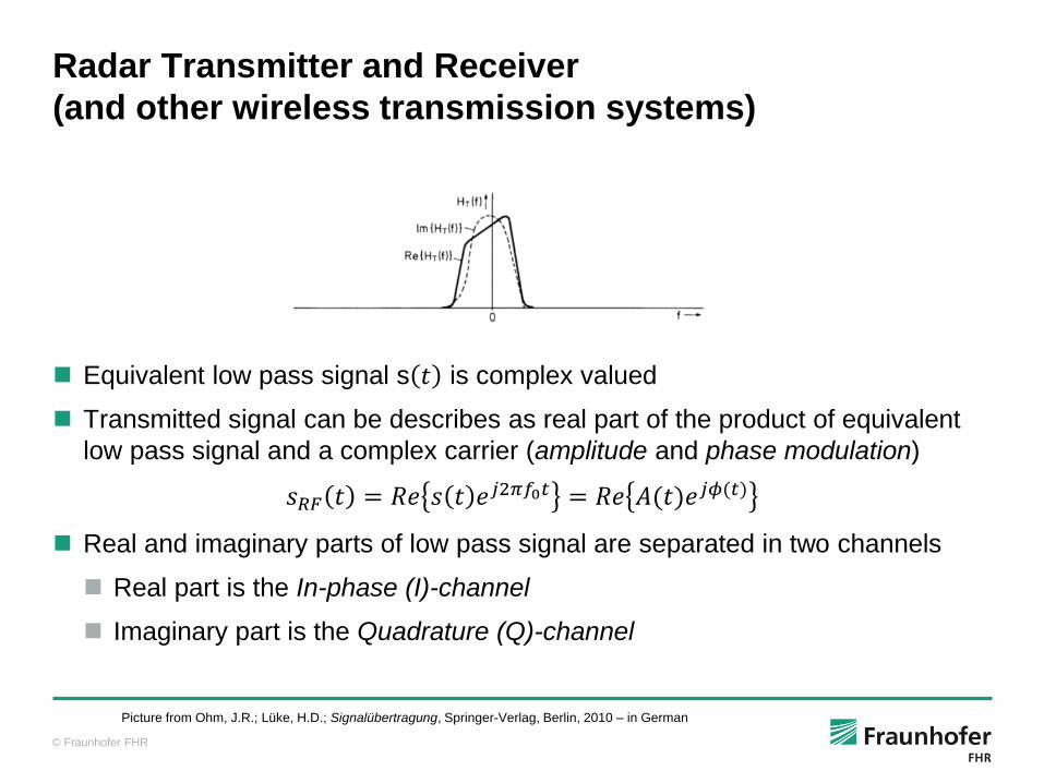
Equivalent low pass signal s 𝑡 is complex valued
Transmitted signal can be describes as real part of the product of equivalent
low pass signal and a complex carrier (amplitude and phase modulation)
𝑠𝑅𝐹 𝑡 = 𝑅𝑒 𝑠 𝑡 𝑒𝑗2𝜋𝑓0𝑡 = 𝑅𝑒 𝐴(𝑡)𝑒𝑗𝜙(𝑡)
Real and imaginary parts of low pass signal are separated in two channels
Real part is the In-phase (I)-channel
Imaginary part is the Quadrature (Q)-channel
Picture from Ohm, J.R.; Lüke, H.D.; Signalübertragung, Springer-Verlag, Berlin, 2010 – in German
© Fraunhofer FHR
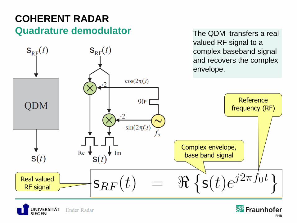
COHERENT RADAR
Quadrature demodulator
Real valued RF signal
Complex envelope, base band signal
Reference frequency (RF)
The QDM transfers a real
valued RF signal to a
complex baseband signal
and recovers the complex
envelope.

© Fraunhofer FHR
The QM transfers the
complex baseband signal
to a real valued RF signal.
COHERENT RADAR
Quadrature modulator
© Fraunhofer FHR
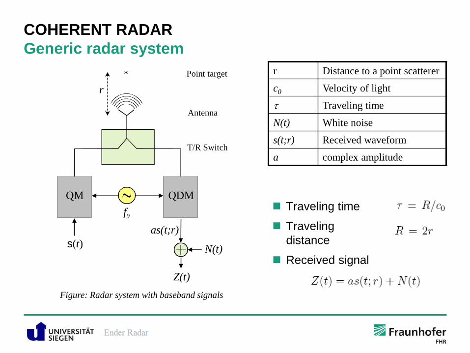
COHERENT RADAR
Generic radar system
Traveling time
Traveling
distance
Received signal
r Distance to a point scatterer
c0 Velocity of light
t Traveling time
N(t) White noise
s(t;r) Received waveform
a complex amplitude
Point target
Antenna
T/R Switch
r
*
QM
s(t)
f0
QDM
as(t;r)
N(t)
Z(t)
Figure: Radar system with baseband signals
© Fraunhofer FHR
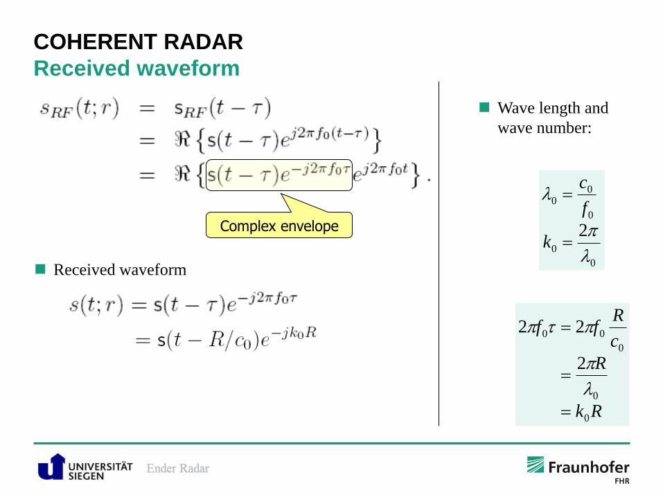
COHERENT RADAR
Received waveform
Complex envelope
Received waveform
Wave length and
wave number:
Rk
R
c
Rff
0
0
0
00
2
22
t
0
0
0
00
2
k
f
c
© Fraunhofer FHR
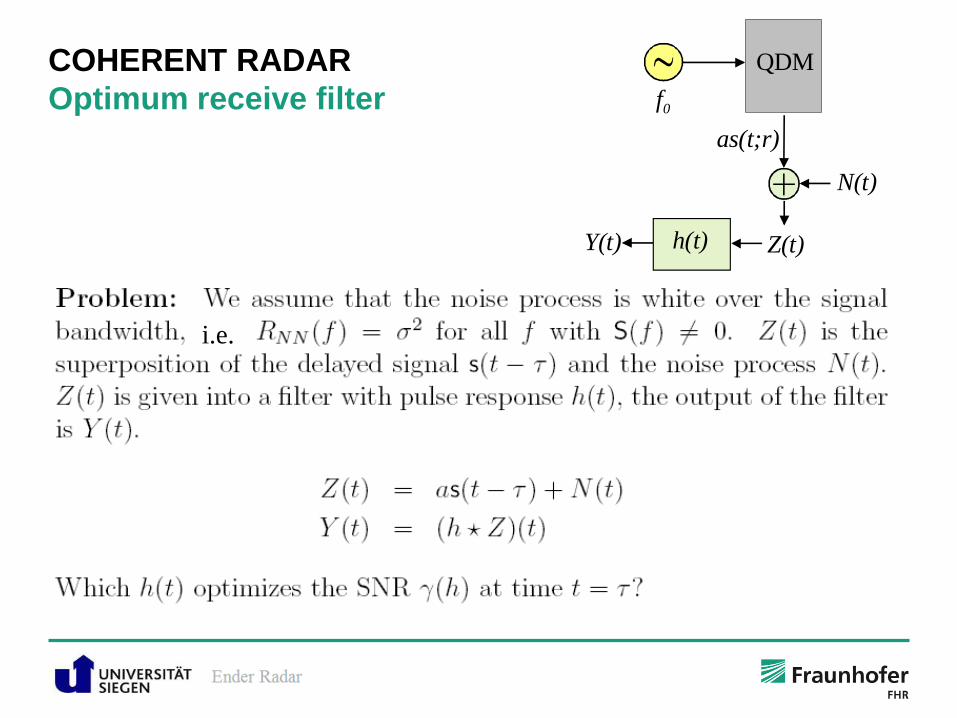
COHERENT RADAR
Optimum receive filter
i.e.
f0
QDM
as(t;r)
N(t)
Z(t)h(t)Y(t)
© Fraunhofer FHR
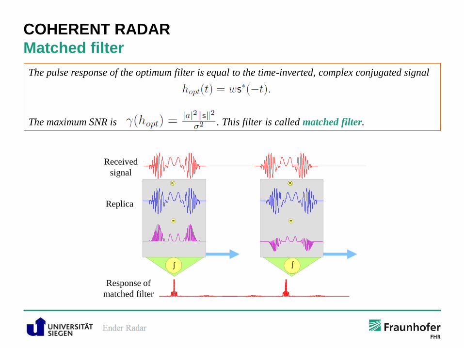
COHERENT RADAR
Matched filter
Received
signal
Replica
Response of
matched filter
The pulse response of the optimum filter is equal to the time-inverted, complex conjugated signal
The maximum SNR is . This filter is called matched filter.

© Fraunhofer FHR
COHERENT RADAR
Point spread function

© Fraunhofer FHR
COHERENT RADAR
Matched filter, point spread function
Reflectivity of three point targets Output of the matched filter
Point spread function
Matched filtering means correlation with the transmit signal. The point spread function is the
reaction of the receive filter to the transmit signal.
The point spread function is equal to the autocorrelation of the transmit signal, if a matched filter
is used.
In this case it is the Fourier back transform of the magnitude-squared of the signal spectrum.
© Fraunhofer FHR
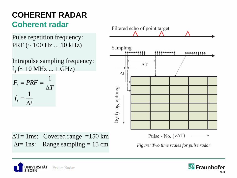
COHERENT RADAR
Coherent radar
Pulse repetition frequency:
PRF (~ 100 Hz ... 10 kHz)
Intrapulse sampling frequency:
fs (~ 10 MHz ... 1 GHz)
tf
TPRFF
s
s
1
1
T= 1ms: Covered range =150 km
t= 1ns: Range sampling = 15 cm Figure: Two time scales for pulse radar

© Fraunhofer FHR
Doppler Effect
Up to now, the radar target was a non-moving isotropic point scatterer
Now it becomes a moving isotropic point scatterer
Movement of target implies Doppler shift on radar signal proportional to the
targets speed
𝑠(𝑡)𝑒𝑗2𝜋𝑓0𝑡 𝑠(𝑡)𝑒𝑗2𝜋 𝑓0+𝑓𝐷 𝑡
Output of matched filter is no longer the autocorrelation of the transmit
signal
Cross correlation between transmitted signal and Doppler shifted receive
signal
𝑝 𝑡 = 𝑠∗ 𝜏 𝑠 𝑡 + 𝜏 𝑑𝜏 𝑝 𝑡, 𝑓𝐷 = 𝑠∗ 𝜏 𝑠 (𝑡 + 𝜏)𝑒𝑗2𝜋𝑓𝐷𝜏𝑑𝜏
© Fraunhofer FHR
Doppler Effect – Ambiguity Function
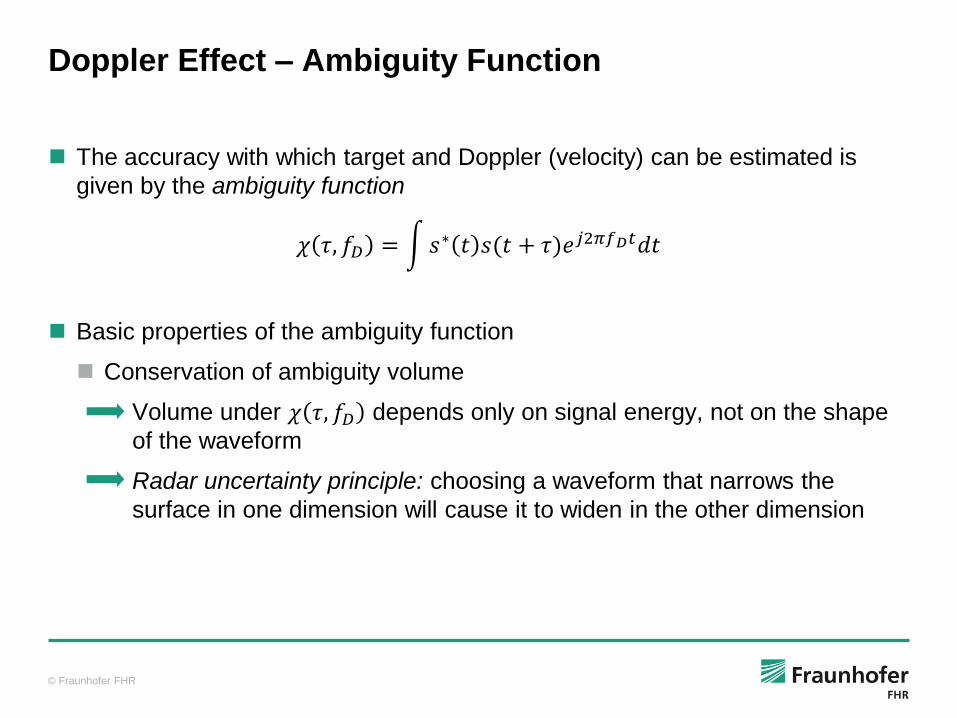
The accuracy with which target and Doppler (velocity) can be estimated is
given by the ambiguity function
𝜒 𝜏, 𝑓𝐷 = 𝑠∗ 𝑡 𝑠(𝑡 + 𝜏)𝑒𝑗2𝜋𝑓𝐷𝑡𝑑𝑡
Basic properties of the ambiguity function
Conservation of ambiguity volume
Volume under 𝜒 𝜏, 𝑓𝐷 depends only on signal energy, not on the shape
of the waveform
Radar uncertainty principle: choosing a waveform that narrows the
surface in one dimension will cause it to widen in the other dimension

© Fraunhofer FHR
Doppler Effect – Ambiguity Function
To determine the range resolution, the frequency domain expression of the
ambiguity function is needed
𝜒 𝜏, 𝑓𝐷 = 𝑆∗ 𝑓 𝑆(𝑓 + 𝑓𝐷)𝑒𝑗2𝜋𝑓𝜏𝑑𝑓
For the range resolution a stationary target (𝑓𝐷 = 0) is considered
𝜒 𝜏, 0 = 𝑆(𝑓) 2𝑒𝑗2𝜋𝑓𝜏𝑑𝑓
Theoretical optimal range resolution is obtained by a Dirac delta function
Such a signal would have infinite energy
Functions broadly supported in the Fourier domain improve the resolution
© Fraunhofer FHR
COHERENT RADAR
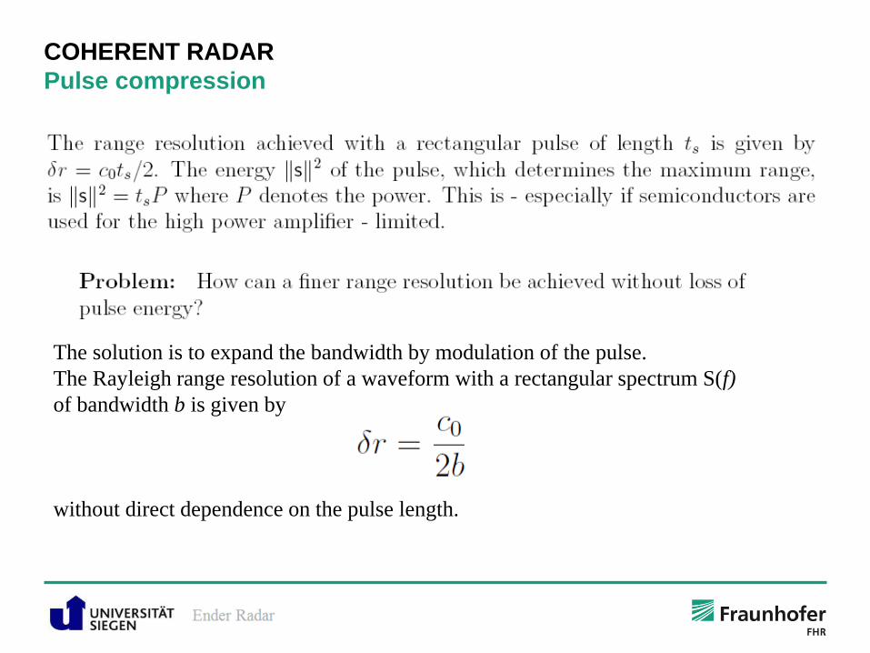
Pulse compression
The solution is to expand the bandwidth by modulation of the pulse.
The Rayleigh range resolution of a waveform with a rectangular spectrum S(f)
of bandwidth b is given by
without direct dependence on the pulse length.
© Fraunhofer FHR
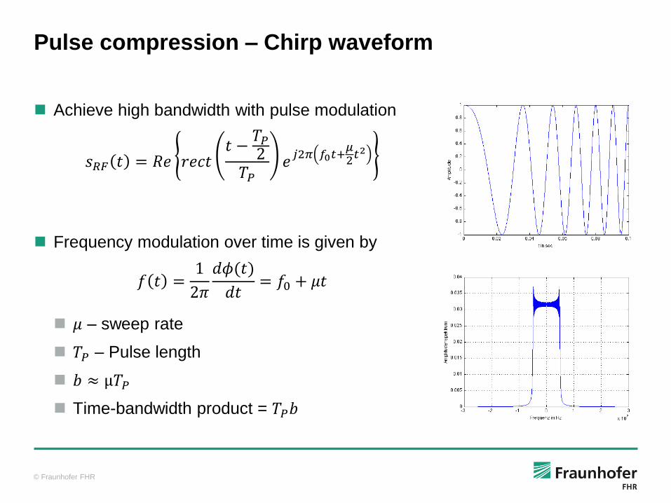
Pulse compression – Chirp waveform
Achieve high bandwidth with pulse modulation
𝑠𝑅𝐹 𝑡 = 𝑅𝑒 𝑟𝑒𝑐𝑡𝑡 −𝑇𝑃2
𝑇𝑃𝑒𝑗2𝜋 𝑓0𝑡+
𝜇2𝑡2
Frequency modulation over time is given by
𝑓 𝑡 =1
2𝜋
𝑑𝜙(𝑡)
𝑑𝑡= 𝑓0 + 𝜇𝑡
𝜇 – sweep rate
𝑇𝑃 – Pulse length
𝑏 ≈ μ𝑇𝑃
Time-bandwidth product = 𝑇𝑃𝑏

© Fraunhofer FHR
t
f
t
f
Chirp
F F-1
act
t|.|2
Spectrum
Power
Spectrum
Compression
result
Pulse compression – Chirp waveform
© Fraunhofer FHR
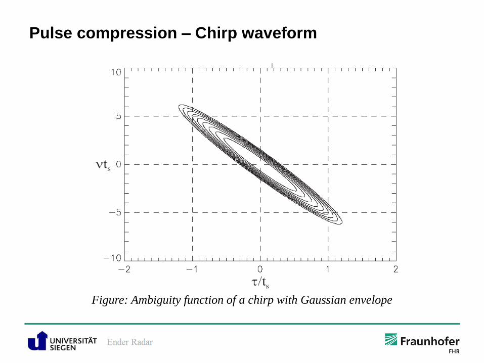
Figure: Ambiguity function of a chirp with Gaussian envelope
Pulse compression – Chirp waveform

© Fraunhofer FHR
SYNTHETIC APERTURE RADAR
Imaging radar (SAR, ISAR) is based on ..
Measurement of range
(pulse compression)
Measurement of range change via phase
(-> cross range resolution)
Relative aspect change of
the scene, the object
necessary
SAR: via motion of the
platform
ISAR: via motion of the target
© Fraunhofer FHR
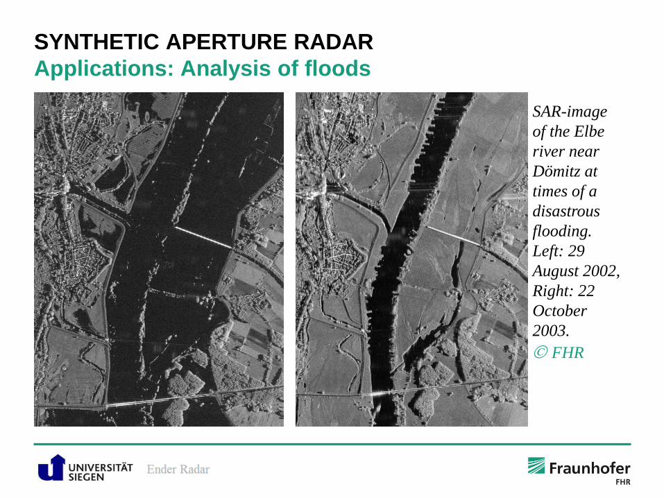
SYNTHETIC APERTURE RADAR
Applications: Analysis of floods
SAR-image
of the Elbe
river near
Dömitz at
times of a
disastrous
flooding.
Left: 29
August 2002,
Right: 22
October
2003.
FHR
© Fraunhofer FHR
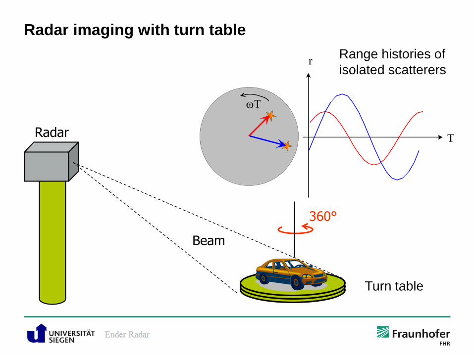
Radar imaging with turn table
Radar
Turn table
Beam
360°
T
rRange histories of
isolated scatterers
© Fraunhofer FHR
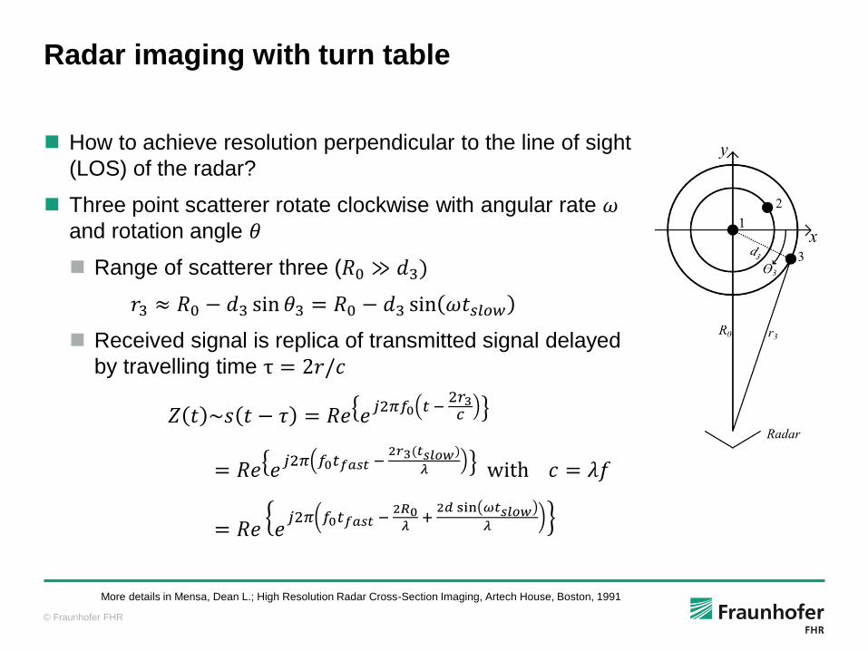
Radar imaging with turn table
How to achieve resolution perpendicular to the line of sight
(LOS) of the radar?
Three point scatterer rotate clockwise with angular rate 𝜔
and rotation angle 𝜃
Range of scatterer three (𝑅0 ≫ 𝑑3)
𝑟3 ≈ 𝑅0 − 𝑑3 sin 𝜃3 = 𝑅0 − 𝑑3 sin 𝜔𝑡𝑠𝑙𝑜𝑤
Received signal is replica of transmitted signal delayed
by travelling time τ = 2𝑟/𝑐
𝑍 𝑡 ~𝑠 𝑡 − 𝜏 = 𝑅𝑒 𝑒𝑗2𝜋𝑓0 𝑡 −
2𝑟3𝑐
= 𝑅𝑒 𝑒𝑗2𝜋 𝑓0𝑡𝑓𝑎𝑠𝑡 −
2𝑟3(𝑡𝑠𝑙𝑜𝑤)
𝜆 with 𝑐 = 𝜆𝑓
= 𝑅𝑒 𝑒𝑗2𝜋 𝑓0𝑡𝑓𝑎𝑠𝑡 −
2𝑅0𝜆 + 2𝑑 sin 𝜔𝑡𝑠𝑙𝑜𝑤
𝜆
More details in Mensa, Dean L.; High Resolution Radar Cross-Section Imaging, Artech House, Boston, 1991
© Fraunhofer FHR
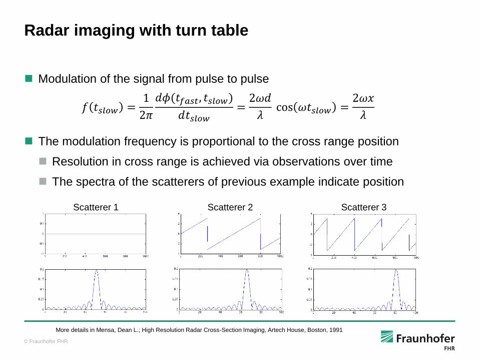
Radar imaging with turn table
Modulation of the signal from pulse to pulse
𝑓 𝑡𝑠𝑙𝑜𝑤 =1
2𝜋
𝑑𝜙(𝑡𝑓𝑎𝑠𝑡, 𝑡𝑠𝑙𝑜𝑤)
𝑑𝑡𝑠𝑙𝑜𝑤=2𝜔𝑑
𝜆 cos 𝜔𝑡𝑠𝑙𝑜𝑤 =
2𝜔𝑥
𝜆
The modulation frequency is proportional to the cross range position
Resolution in cross range is achieved via observations over time
The spectra of the scatterers of previous example indicate position
Scatterer 1 Scatterer 2 Scatterer 3
More details in Mensa, Dean L.; High Resolution Radar Cross-Section Imaging, Artech House, Boston, 1991
© Fraunhofer FHR
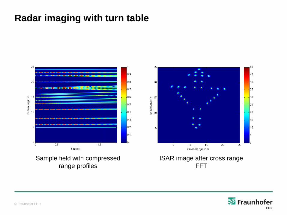
Radar imaging with turn table
Sample field with compressed
range profiles
ISAR image after cross range
FFT

© Fraunhofer FHR
Questions…
or Ideas?