Introduction to Queueing Theory

Motivation

First developed to analyze statistical behavior of phone switches.

Queueing Systems

model processes in which customers arrive.

wait their turn for service.

are serviced and then leave.

Examples

supermarket checkouts stands.

world series ticket booths.

doctors waiting rooms etc..

Five components of a Queueing system:

1. Interarrival-time probability density function (pdf)

2. service-time pdf 3. Number of servers 4. queueing discipline 5. size of queue.

ASSUME

an infinite number of customers (i.e. long queue does not reduce customer number).

Assumption is bad in :

a time-sharing model.with finite number of customers.

if half wait for response, input rate will be reduced.

Interarrival-time pdf

record elapsed time since previous arrival.

list the histogram of inter-arrival times (i.e. 10 0.1 sec, 20 0.2 sec ...).

This is a pdf character.

Service time

how long in the server? i.e. one customer has a shopping cart full the other a box of cookies.

Need a PDF to analyze this.

Number of servers

banks have multiserver queueing systems.

food stores have a collection of independent single-server queues.

Queueing discipline

order of customer process-ing.

i.e. supermarkets are first-come-first served.

Hospital emergency rooms use sickest first.

Finite Length QueuesSome queues have finite length: when full customers are rejected.

ASSUME

infinite-buffer. single-server system with first-come.

first-served queues.

A/B/m notation

A=interarrival-time pdfB=service-time pdfm=number of servers.

A,B are chosen from the set:

M=exponential pdf (M stands for Markov)

D= all customers have the same value (D is for deterministic)

G=general (i.e. arbitrary pdf)

Analysibility

M/M/1 is known. G/G/m is not.

M/M/1 system

For M/M/1 the probability of exactly n customers arriving during an interval of length t is given by the Poisson law.

Poisson’s Law

Pn (t )(t)n

n!e t (1)

Poisson’s Law in Physicsradio active decay –P[k alpha particles in t seconds]– = avg # of prtcls per second

Poisson’s Law in Operations Researchplanning switchboard sizes –P[k calls in t seconds]– =avg number of calls per sec

Poisson’s Law in Biologywater pollution monitoring –P[k coliform bacteria in 1000 CCs]– =avg # of coliform bacteria per cc

Poisson’s Law in Transportationplanning size of highway tolls –P[k autos in t minutes]– =avg# of autos per minute

Poisson’s Law in Opticsin designing an optical recvr –P[k photons per sec over the surface of area A] – =avg# of photons per second per unit area

Poisson’s Law in Communications in designing a fiber optic xmit-rcvr link –P[k photoelectrons generated at the rcvr in one second] – =avg # of photoelectrons per sec.

- Rate parameter =event per unit interval (time distance volume...)

Analysis

Depend on the condition:

we should get 100 custs in 10 minutes (max prob).

interarrival rate 10 cust. per min

n the number of customers = 100

To obtain numbers with a Poisson pdf, you can write a program:

Acceptance Rejection Method

Prove:

Poisson arrivals gene-rate an exponential interarrival pdf.

The M/M/1 queue in equilibrium

queue

server

State of the system:

There are 4 people in the system.

3 in the queue. 1 in the server.

Memory of M/M/1:

The amount of time the person in the server has already spent being served is independent of the probability of the remaining service time.

Memoryless

M/M/1 queues are memoryless (a popular item with queueing theorists, and a feature unique to exponential pdfs).P kequilibrium prob .

that there are k in system

Birth-death system

In a birth-death system once serviced a customer moves to the next state.

This is like a nondeterminis-tic finite-state machine.

State-transition Diagram

The following state-transition diagram is called a Markov chain model.

Directed branches represent transitions between the states.

Exponential pdf parameters appear on the branch label.

Single-server queueing system

0 1 2 k-1 k k+1...

Po P1 P k-1 P k

P k P k+1P1 P2

Symbles:

mean arrival rate (cust. /sec)

mean service rate (cust./ sec)

P0mean number of transitions/ secfrom state 0 to 1

P1mean number of transitions/ sec

from state 1 to 0

States

State 0 = system empty

State 1 = cust. in server

State 2 = cust in server, 1 cust in queue etc...

Probalility of Given State

Prob. of a given state is invariant if system is in equilibrium.

The prob. of k cust’s in system is constant.

Similar to AC

This is like AC current entering a node

is called detailed balancing

the number leaving a node must equal the number entering

Derivation

P0 P1

P1 P0

P1 P2

P 2 P1

3

3a

4

4a

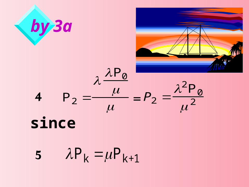
by 3a

P 2

P0

P2 2P 0

2

P k P k+1

=4

since

5

then:

P k kP0

k kP06

where = traffic intensity < 1

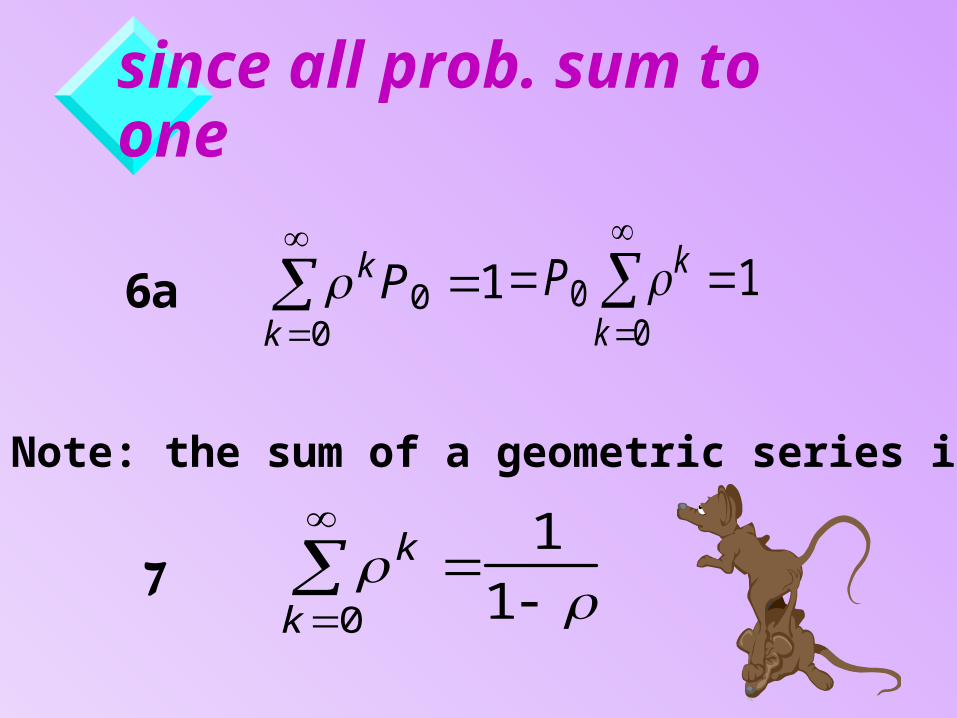
since all prob. sum to one

kP0k0

1P0 kk0

16a

Note: the sum of a geometric series is

kk0

1

1 7

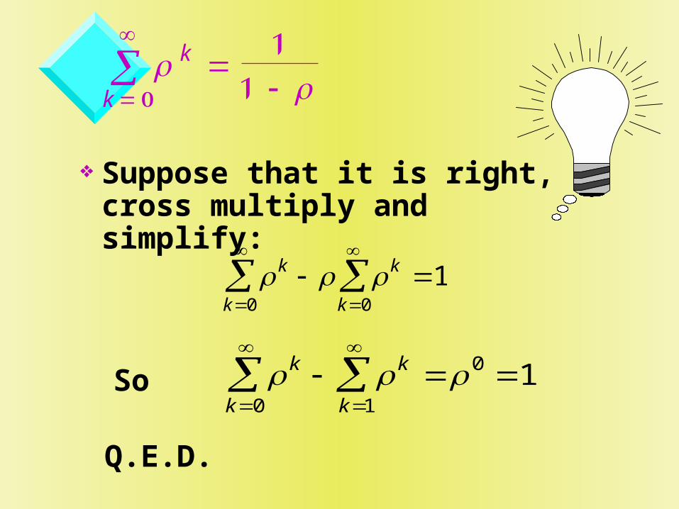
Suppose that it is right, cross multiply and simplify:

k

k 0

1

1

kk0

kk0

1

kk0

kk1

0 1SoQ.E.D.

subst 7 into 6a

P0

1 1

P0 kk0

16a

7a and

P0 1 =prob server is empty

7b

subst into

P k kP0

k kP06

yields:

P k (1 ) k8

Mean value:

let N=mean number of cust’s in the system

To compute the average (mean) value use:

E[k ] kPkk0

8a

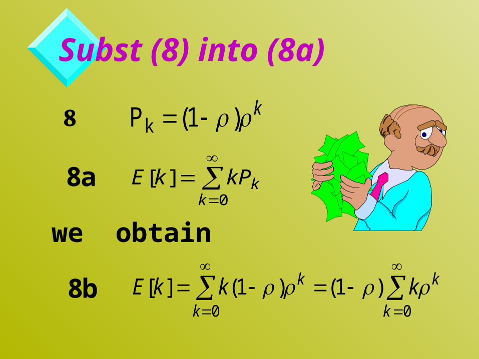
Subst (8) into (8a)

P k (1 ) k

E[k ] kPkk0

E[k ] k(1 ) kk0

(1 ) k kk0

8

8a

8b

we obtain

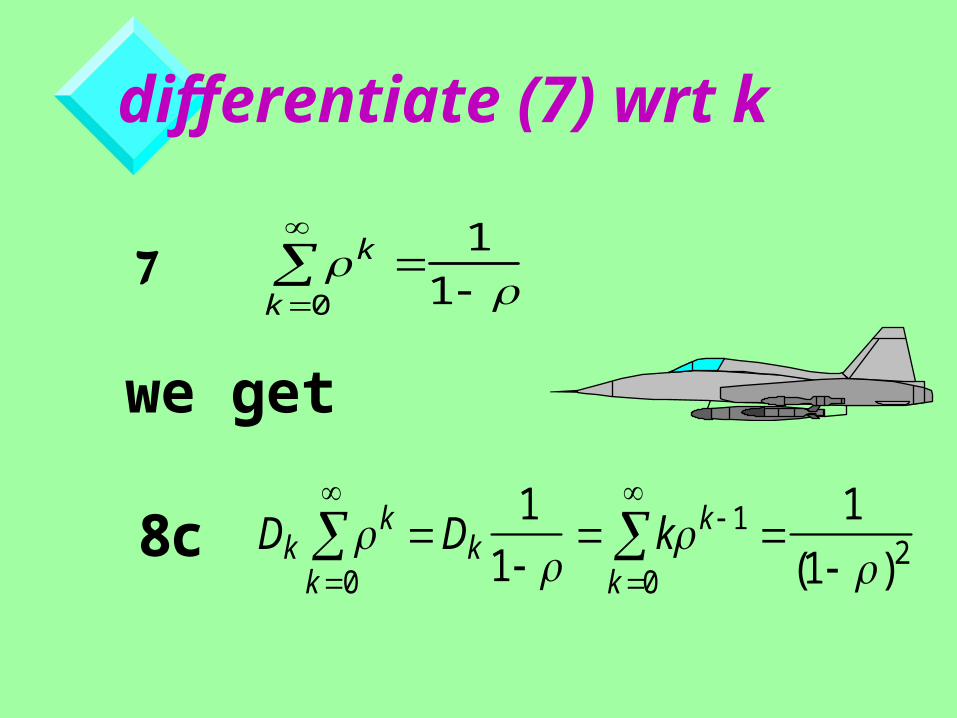
differentiate (7) wrt k

kk0

1

1

Dk kk0

Dk1

1 k k 1

k0

1

(1 )2

7

we get

8c

multiply both sides of (8c) by

kkk0

(1 )2

E[k ] N (1 )

(1 )2

(1 )

8d

9

Relationship of , N

0 0.2 0.4 0.6 0.8 10

20

40

60

80

rho

as r approaches 1, N grows quickly.

T and

T=mean interval between cust. arrival and departure, including service.

mean arrival rate (cust. /sec)

Little’s result:

In 1961 D.C. Little gave us Little’s result:

T N

/ 1

1 / 1

1

10

For example:

A public bird bath has a mean arrival rate of 3 birds/min in Poisson distribution.

Bath-time is exponentially distributed, the mean bath time being 10 sec/bird.

Compute how long a bird waits in the Queue (on average):

0.05 cust / sec = 3 birds / min * 1 min / 60 sec

= mean arrival rate

= 0.1 bird / sec = 1 bird

10 sec

= mean service rate

Result:

So the mean service-time is 10 seconds/bird =(1/ service rate)T

1

1

0.1 0.0520sec

for wait + service

Mean Queueing Time

The mean queueing time is the waiting time in the system minus the time being served, 20-10=10 seconds.

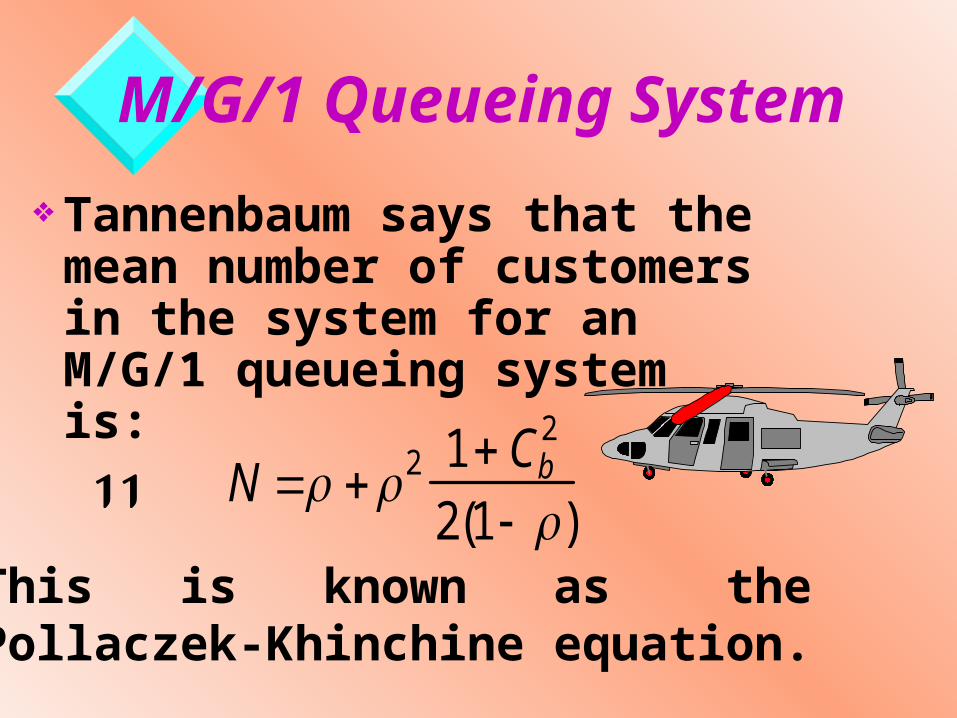
M/G/1 Queueing System

Tannenbaum says that the mean number of customers in the system for an M/G/1 queueing system is:

N 2 1 Cb2

2(1 )11

This is known as the Pollaczek-Khinchine equation.

What is Cb

Cb standard deviation

mean

of the service time.

Note:

M/G/1 means that it is valid for any service-time distribution.

For identical service time means, the large standard deviation will give a longer service time.

Introduction to Queueing Theory