Introduction to Quantum Optics I

Carsten Henkel

Universitat Potsdam, WS 2019/20

The preliminary programme for this lecture:

Motivation: experiments in Potsdam and elsewhere

I Interaction between light and atoms (light and matter)

— relevant observables, statistics

— the model of a two-level atom, a two-level medium

— Bloch equations

— quantum states of one qubit

II Photons – field quantization

— elementary scheme with a mode expansion

— states of the radiation field: Fock, coherent, thermal, squeezed;distribution functions in phase space

— Jaynes-Cummings-Paul model (collapse and revival)

— about spontaneous emission, quantum noise and vacuum energies

Outlook SS 2020: quantum optics II

— master equations, photodetection

— beamsplitter, homodyne detection

— open systems, “system + bath” paradigm

— quantum theory of the laser and the micromaser

— correlations and fluctuations, spectral characterization

— problems of current interest:two-photon interference, intensity correlationsvirtual vs real photons, strong coupling

These notes are a merger of previous years and contain more material thanwas actually delivered in WS 2019/20.

1

Motivation

List of experiments, some of them performed at University of Potsdam. Try toanswer the question: is this a quantum optics experiment? do we need quantumoptics to understand it?

— A laser pulse is sent on a metallic surface and is (partially) absorbed there(see Problem 1.1(iv)).

— Small metallic particles are covered with a layer of quantum dots and de-posited on a substrate. The absorption spectrum shows two peaks.

— When photons are absorbed in a semiconductor, they may create excitonsthat diffuse by hopping through the sample. The excitons can dissociateand generate charge carriers that create a current (solar cell).

— A femto-second short pulse is absorbed in a molecular beam and generatesvibrational wavepackets.

— A polymer film is irradiated with an light pattern and develops a deforma-tion that can be measured with a scanning microscope.

— A laser beam is exciting an optical cavity where one mirror is mobile: it ispushed a little due to radiation pressure. By adjusting the frequency of thelaser, the motion of the mirror is cooled down.

— An intense laser is focused into a crystalline material and generates pairs ofphotons (also known as biphotons). The polarizations of the biphoton part-ners is uncertain, but anti-correlated with certainty: when one partner ofthe biphoton is polarized horizontally, the other has a vertical polarization–– and the other way around.

— When UV light is sent onto a metal, it generates free electrons whose en-ergy increases linearly with the light frequency (photoelectric effect, pho-todetector). In theoretical chemistry and surface physics, this effect is mod-elled with a classical electromagnetic field inserted into the Schrodingerequation for the metallic electrons.

2

Contents

1 Matter-light interaction 41.1 Atomic physics . . . . . . . . . . . . . . . . . . . . . . . . . . . . 4

1.1.1 Atom-light interaction . . . . . . . . . . . . . . . . . . . . 61.1.2 Selection rules . . . . . . . . . . . . . . . . . . . . . . . . 91.1.3 Two-level atoms . . . . . . . . . . . . . . . . . . . . . . . 101.1.4 Resonance approximation . . . . . . . . . . . . . . . . . . 111.1.5 Rabi oscillations . . . . . . . . . . . . . . . . . . . . . . . 17

1.2 Quantum mechanics of two-level system . . . . . . . . . . . . . . 191.2.1 Atom Hamiltonian . . . . . . . . . . . . . . . . . . . . . . 191.2.2 Schrodinger equation . . . . . . . . . . . . . . . . . . . . 211.2.3 Resonance approximation . . . . . . . . . . . . . . . . . . 221.2.4 Rabi oscillations . . . . . . . . . . . . . . . . . . . . . . . 23

1.3 Dissipation and open system dynamics . . . . . . . . . . . . . . . 251.3.1 Spontaneous emission . . . . . . . . . . . . . . . . . . . . 251.3.2 Bloch equations . . . . . . . . . . . . . . . . . . . . . . . . 261.3.3 Limit of rate equations . . . . . . . . . . . . . . . . . . . . 271.3.4 The Bloch-Lorenz model . . . . . . . . . . . . . . . . . . . 29

1.4 More notes on mixed states and dissipation . . . . . . . . . . . . 301.4.1 State of a two-level system . . . . . . . . . . . . . . . . . . 301.4.2 Quantum jump approach for a two-level system . . . . . . 351.4.3 Lindblad master equation . . . . . . . . . . . . . . . . . . 38

1.5 Spin language and Bloch sphere . . . . . . . . . . . . . . . . . . . 391.5.1 Bloch vector . . . . . . . . . . . . . . . . . . . . . . . . . . 391.5.2 Bloch dynamics . . . . . . . . . . . . . . . . . . . . . . . . 40

1.6 Outlook: light-matter interaction . . . . . . . . . . . . . . . . . . 43

3

Chapter 1

Matter-light interaction

1.1 Atomic physicsThese notes go a bit beyond the material covered in WS 19/20.

An atom can be modelled as a collection of charged point particles. Thesimplest Hamiltonian one can write is therefore

HA =X

↵

p2

↵

2M↵+

1

2

X

↵ 6=�

e↵e�

4⇡"0|x↵ � x�|(1.1)

where ↵ labels the particles, M↵, e↵ are their masses and charges. We try touse in this lecture SI units. (In cgs units, drop the 4⇡"0.) The interaction termcorresponds to the electrostatic (or Coulomb) field created by the charges.

More advanced atomic models adopt a relativistic viewpoint, take into ac-count the electron spin, the magnetic field created by the motion of the particles,the corresponding spin-orbit interaction, the spin-spin coupling, the hyperfine in-teraction etc. Theoretical atomic physics computes all these corrections to theenergy levels and matrix elements ‘from first principles’ (see the textbook byHaken & Wolf (2000), for example). Typically, no simple analytical results canbe found for atoms with more than two or three electrons, say.

For our purposes, we are not interested in so much detail. Instead, we use asimplified description of the atom states that captures their essential properties.Good examples are atoms with a single electron in the outer shell (the alkalineseries), as listed in table 1.1. Their energy levels are to a good approximation

4

hydrogen Hlithium Lisodium Natrium Napotassium Kalium Krubidium Rbcesium Csfrancium Fr

n l = 0 l = 1 l = 2 . . .. . . . . . . . . . . . . . .3 3s 3p 3d2 2s 2p1 1s

Table 1.1: Left: the series of alkaline atoms. Right: Spectroscopic notation forenergy levels of hydrogen-like atoms.

given by a modified Balmer formula

Enl = �e2

8⇡"0a0 (n+ �l)2= �

Ryd

(n+ �l)2,

n = 1, 2 . . .

l = 0, . . . n� 1(1.2)

The Bohr radius a0 = 4⇡"0h2/me

2⇡ 0.5 A gives the typical size of the electron

cloud, and the ‘quantum defect’ �l lifts the degeneracy of the hydrogen levels.Theenergy scale is given by the Rydberg constant Ryd ⇡ 13.6 eV.

The charge Z|e| of the nucleus enters the Balmer formula via the quantum defects �l. In fact,the outer electron ‘sees’ the nucleus screened by the core electrons. This gives a Coulombpotential as for the hydrogen atom, with some modifications due to the core electrons. Theseare responsible for the lifted degeneracy between the l states.

The frequency of electromagnetic radiation emitted by atoms in a process|ii ! |fi is given according to Bohr by

!if =Ei � Ef

h(1.3)

For two typical energy levels Ei,f , h!if is also of the order of 1Ryd. If we computethe wavelength of the corresponding electromagnetic radiation, we find

�if ⇠2⇡hc

Ryd=

4⇡

↵fs

a0 � a0 (1.4)

fine structure constant ↵fs =e2

4⇡"0hc⇡

1

137, (1.5)

which is much longer than the typical size of the atom (the Bohr radius givesthe extension of the electronic orbitals). For typical light fields, the atom thus

5

appears like a pointlike object. This property justifies the ‘long wavelength ap-proximation’ that simplifies the Hamiltonian for the atom–light interaction.

Another way of looking at the result (1.4) is to interpret the inverse finestructure constant, ↵�1

fs= c(4⇡"0h/e2) as the ratio between the speed of light

c and the typical velocity for an electron in the Hydrogen atom (the naturalvelocity scale in the so-called ‘atomic units’). We see that this velocity is only afew percent of c, hence we expect that the non-relativistic description we haveused so far is a good approximation.

1.1.1 Atom-light interaction

Minimal coupling

According to the rules of electrodynamics, the interaction between a collection ofcharges with a given electromagnetic field is described by the ‘minimal coupling’Hamiltonian. This corresponds to the replacement p↵ 7! p↵ � e↵A(x↵, t) whereA(r, t) is the vector potential. In this chapter, this is a given time-dependentfunction. It will become an operator when the field is quantized. In addition,there is the potential energy due to an ‘external’ scalar potential �ext(x, t), so thatwe get

HAF =X

↵

(p↵ � e↵A(x↵, t))2

2M↵+

1

2

X

↵ 6=�

e↵e�

4⇡"0|x↵ � x�|+X

↵

e↵�ext(x↵, t). (1.6)

The minimal coupling prescription is related to the freedom of choosing thephase reference of the wave function, as is seen in more detail in the exercises.

Remark. This freedom is also called ‘local U(1) gauge invariance’ because phase factors formthe unitary group U(1). Local changes in the phase of the wave function generate terms in theSchrodinger equation that can be combined with gauge transformations for the electromagneticpotentials. This connection to the electromagnetic gauge transformations is of great importancefor quantum field theory. It allows to construct the coupling to the electromagnetic field fromthe symmetry properties of the quantum fields. For example, there are theories where electronsand neutrinos are combined into a two-component field, and the interactions are invariant underSU(2) transformations that mix these two, plus U(1) transformations of the phase common to thetwo components. The group SU(2)⇥U(1) is four-dimensional and has four ‘generators’. Each ofthem corresponds to a vector potential that interacts with the two-component field. In additionto the standard electromagnetic potential (the ‘photon’), there are interactions associated to the‘massive vector bosons’, called W

± and Z0. They convey the ‘weak interaction’ that is responsible

6

for � decay. More details in any book on quantum field theory. I sometimes use the one byItzykson & Zuber (2006).

When the minimal coupling Hamiltonian (1.6) is expanded to lowest orderin the charges e↵, we obtain the so called ‘p · A’ interaction

Hint = �X

↵

e↵

2M↵{p↵ ·A(x↵, t) +A(x↵, t) · p↵}+

X

↵

e↵�ext(x↵, t). (1.7)

In the Coulomb gauge where r·A = 0, the ordering of the operators is irrelevant.This interaction is linear in the vector potential, but there is also a second-order(or ‘diamagnetic’) term

Hdia =X

↵

e2

↵A2(x↵, t)

2M↵(1.8)

When calculations are pushed to second order in the p · A-coupling, the dia-magnetic interaction must be included as well, for consistency. This makes the‘book-keeping’ in perturbation theory complicated.

Gauge transformation. There are essentially two schools that treat the scalar potential in verydifferent ways.

(1) Either one is interested in electromagnetic fields on short scales compared to the wave-length (called “non-retarded limit”). Then one can ignore the vector potential and use only thescalar potential �ext to describe the matter-field interaction. This applies, for example, to theinteraction of atoms or matter with electrons (scattering experiments).

(2) Or the wavelength is an important scale. Then one can even choose a gauge where�ext = 0, and only the vector potential is nonzero.

Sometimes a mixture of the two schemes is needed, for example when light creates chargecarriers, like in semiconductors or in the photoelectric effect.

Electric dipole coupling

A simpler approach is possible, however. We first make the approximation thatthe field varies slowly on the scale of the displacements x↵ of the charges in theatom. Then we can replace, to lowest order, A(x↵, t) ⇡ A(R, t) where R is theatomic center of charge. This is called the ‘long-wavelength approximation’ thatis well justified for fields near-resonant with typical atomic transitions. Withinthis approximation, we can find a simpler interaction Hamiltonian that is linearin the electromagnetic field. It is called the ‘d · E’ coupling and is strictly linear

7

in the electric field:

Hint = �d · E(R, t),

d =X

↵

e↵(x↵ �R), (1.9)

where d is the electric dipole moment of the atom relative to R. This version ofthe d ·E interaction can be derived from the minimal coupling Hamiltonian witha gauge transformation (see the exercises) from the minimal coupling Hamil-tonian in the long-wavelength approximation, without invoking an additionalapproximation.

Gauge transformation. Change from the vector potential A(x, t) to

A0(x, t) = A(x, t)�r�(x, t), �(x, t) = (x�R) ·A(R, t) (1.10)

where �(x, t) is called the ‘gauge function’. It ensures that A0(R, t) = 0 at all times. Since thegauge function is time-dependent, the scalar potential also changes:

�0(x, t) = �(x, t) + @t�(x, t) = �(x, t) + (x�R) · @tA(R, t) (1.11)

If we simply insert these ‘new potentials’ into the minimal coupling Hamiltonian, we get

H0dia = 0, H

0int = +

X

↵

e↵ {�ext(x↵, t) + (x↵ �R) · @tA(R, t)} (1.12)

Note that the diamagnetic term cancels without further approximation. We expand the scalarpotential for small x↵ �R and get

H0int = +�ext(R, t)

X

↵

e↵ +X

↵

e↵(x↵ �R) · {r�ext(R, t) + ·@tA(R, t)} (1.13)

The first term cancels if the system of charges is globally neutral. In the second term, we rec-ognize the expression of the electric field E(R, t) in terms of the potentials. Hence we find theelectric dipole Hamiltonian (1.9).

The advantages of the electric dipole coupling are: the atom couples directlyto the field; there is no quadratic interaction term. One must not forget thatbetween the two interactions, the wave function (the atomic state) differs by aunitary transformation. Otherwise, some matrix elements or transition rates maycome out differently. This issue is discussed in great detail in the book ‘Molec-ular Quantum Electrodynamics’ by Craig & Thirunamachandran (1984) and inChap. IV of ‘Photons and Atoms – Introduction to Quantum Electrodynamics’ byCohen-Tannoudji & al. (1987).

8

1.1.2 Selection rules

Since the electric dipole moment determines the interaction with the light field,a few remarks on its matrix elements are in order. We take as a starting pointthe basis of the stationary states of an atom, described by the Hamiltonian (1.1).These states are typically described by quantum numbers like parity, angular mo-mentum etc. The ‘selection rules’ specify for which states we know by symmetrythat the matrix elements of the electric dipole moment vanish. In that case, thecorresponding states are not connected by an ‘electric dipole transition’, or thetransition is ‘dipole-forbidden’.

Parity. We say that a state |ai has a defined parity Pa = ±1 when the electronicwave function ({x↵}) “transforms like” Pa ({x↵}) when all coordinates aretransformed as x↵ 7! �x↵. This means that

(P )({�x↵}) = ({�x↵}) = Pa ({x↵}) (1.14)

where (P ) denotes the action of the parity operator on the wave function.1 Ifnow |ai has a well-defined parity, then it is easy to show that ha|d|ai = 0 (seelecture). In addition, the matrix element ha|d|bi is only nonzero when |ai and |bi

have different parity. This is an example of a “selection rule”. It provides a simpleargument to exclude certain transitions from happening under the electric-dipolecoupling. We shall see below that an off-diagonal matrix element like ha|d|bi isessential when one wants to induce a “quantum jump” from one level to anotherwith light.

Energy. Selection rules often arise when the system has certains symmetries.See a few examples below. The simplest symmetry is “translation in time”, i.e.,the system Hamiltonian does not depend on time. We then know from classicalmechanics that energy is a conserved quantity. This is also true in quantummechanics and quantum optics. The corresponding selection rule for atom-lightinteraction is the Bohr-Sommerfeld rule for the photon (angular) frequency !

that can induce a transition between two levels |ai and |bi:

h! = |Eb � Ea|. (1.15)1In the simple one-dimensional problems you remember from Quantum Mechanics I, wave

functions that are ‘even’ or ‘odd’ have a well-defined parity. But there are also wave function thatare neither even nor odd. One says that these do not have a well-defined parity.

9

This formula is in fact one of the birth certificates of quantum theory – remem-ber that quantum mechanics was developed to explain the discrete frequenciesobserved in the radiation spectra of atoms.

Angular momentum. If there is no electron spin, this is given by l, and by j = l±12 for hydrogen-

like atoms where one spin of a non-paired electron is present. The vector operator d transformsunder rotation like a spin 1 (there are three different basis vectors). One can introduce a basiseq (q = �1, 0, 1) that are eigenvectors of L3 as well and write d =

Pq dqeq. The product eq|l,mi

then is an eigenstate of L3 with eigenvalue q +m. Therefore, the matrix element with |l0,m

0i is

only nonzero when m0 = q +m. We find the selection rule

|m�m0| 1.

In addition, the product states eq|l,mi can be expanded onto eigenstates of L2. The rules for the‘addition of angular momentum’ imply that only angular momenta l

0 = l� 1, l, l+1 occur in thisexpansion. This gives the selection rule

|l � l0| 1.

Total momentum. An atom that is in a plane wave state regarding its centre-of-mass motion,with momentum P receives an additional momentum hk when a photon from a plane electro-magnetic wave with wave vector k is absorbed. The corresponding ‘recoil velocity’ hk/M is ofthe order of a few mm/s to a few cm/s for typical atoms. The atomic recoil plays an importantrole for atom deceleration and cooling with laser light.

1.1.3 Two-level atoms

For the rest of this lecture, it will be sufficient to write the atomic Hamiltonianin the form

HA =X

n

En|nihn|, (1.16)

where the states |ni are the stationary states corresponding to the energy eigen-value En. But even this form is too complicated: it contains too many termswhen dealing with near-resonant laser light. This is the setting we shall focus onhere. One can then retain only a few states to describe the atom.

Two-level observables

Atomic Hamiltonian. The standard notation for the two states is |gi for theground state and |ei for the excited state. The Bohr frequency is often written

10

!A = !e�!g > 0. The atomic energy levels are often referenced to a zero energylying between both states, this gives:

HA =h!A

2|eihe|�

h!A

2|gihg| (1.17)

It is also useful to identify the two-dimensional Hilbert space of the two-levelatom with the 2, using the basis vectors (1, 0)T $ |ei and (0, 1)T $ |gi. TheHamiltonian then becomes the diagonal matrix

HA =h!A

2

0

@ 1 0

0 �1

1

A =h!A

2�3 (1.18)

where �3 is the third Pauli matrix. Indeed, it is obvious that a two-dimensionalHilbert space can be identified with the Hilbert space of a spin 1/2.

Observables energy, inversion, dipole.

d = dge� + d⇤ge�

† = dge|gihe|+ d⇤ge|eihg| (1.19)

where the vector of matrix elements of the dipole operator is dge = hg|d|ei. Onlyoff-diagonal matrix elements because of the parity selection rule.

1.1.4 Resonance approximation

Interaction Hamiltonian

The interaction with a monochromatic laser field can be described by the Hamil-tonian

H = HA � d · E(t) (1.20)

E(t) = E e�i!Lt + c.c.

d = dge|gihe|+ h.c.

where the complex vector E gives the amplitude of the electric field. It is evalu-ated at the position of the atom, we drop this dependence here. The laser (an-gular) frequency is !L. The term E e�i!Lt is called the ‘positive frequency part’ ofthe field: its time evolution is the same as for a solution of the time-dependentSchrodinger equation (with positive energy h!L).

11

We re-write Eq.(1.20) in terms of two separately hermitean operators

�d · E(t) =h

2

⇣⌦ e�i!Lt|eihg|+ h.c.

⌘

+h

2

⇣⌦0 ei!Lt|eihg|+ h.c.

⌘(1.21)

h⌦

2= �d

⇤ge · E, ( Rabi frequency ) (1.22)

where ⌦ is a complex-valued frequency, and ⌦0 has a similar expression asEq.(1.22). (We follow the Paris convention and notation for ⌦.)

If the field is quantized, Eq.(1.20) applies in similar form in the interaction picture and involvesphoton annihilation operators aL in place of the complex amplitude E (and creation operatorsa†L in place of E⇤. The fully quantized interaction Hamiltonian is derived from the quantized

field operator and takes the form:

�d(t) ·E(t) 7!

�

X

k

Ek

⇣ak(t)fk · d(t) + a

†k(t)f

⇤k · d(t)

⌘(1.23)

where Ek =ph!k/(2"0V ) is the electric field amplitude at the one-photon level and fk = fk(R)

is the normalized mode function, evaluated at the position R of the atom. We have writtenEq.(1.23) in the “interaction picture” where all operators carry their “free” time dependence.For the photon annihilation operator ak(t) = ak e�i!kt, which is the operator in the Heisenbergpicture under the free field Hamiltonian. The time dependence of the (freely evolving) dipoleoperator is given by d(t) = exp(iHAt)d exp(�iHAt).

In order to examine what happens to an atom illuminated by a laser field, wemake the Ansatz

| (t)i = ce(t) e�i!t/2

|ei+ cg(t) e+i!t/2

|gi (1.24)

where the frequency ! is chosen later. The amplitudes describe the two-level sys-tem in a picture that differs from the usual choice ce(t), cg(t). The Schrodingerequation for ce contains a correction term because of the time-dependent expo-nential. One gets

ih@tce =

Ee �h!

2

!

ce +h

2⌦ e�i(!L�!)t

cg

+h

2⌦0 ei(!L+!)t

cg (1.25)

Now, we can take the choice Ee = 1

2h!A for the excited state energy. There are

now two “natural choices” for !:

12

(1) interaction picture: ! = !A, and the first term disappears. The time de-pendence of ce is then only due to the atom-laser interaction. This pictureis suitable for perturbation theory.

(2) rotating frame: ! = !L, and the second term becomes time-independent.This picture is suitable for concrete calculations in quantum optics, oncewe have convinced outselves what is the meaning of the third term.

Time-dependent perturbation theory

We now make the choice (1) of the interaction picture and solve the equation force with the help of time-dependent perturbation theory. This proceeds by iden-tifying the interaction Hamiltonian as a “small term” and by counting ascendingpowers.

At the order zero, HA is the only Hamiltonian. Keeping in mind the choice! = !A, Eq.(1.25) reduces to

@tc(0)

e = 0, @tc(0)

g = 0 (1.26)

where the equation for cg is similar to Eq.(1.25). As expected from the analogy tothe time-dependent Schrodinger equation (for the “free” atom), the amplitudesare constants at order zero. The natural initial condition “atom is in state |gi

translates intoc(0)

e (t) = 0, c(0)

g (t) = 1. (1.27)

To the first order, we get from Eq.(1.25)

ih@tc(1)

e =h

2⌦ e�i(!L�!A)t

c(0)

g +h

2⌦0 ei(!L+!A)t

c(0)

g (1.28)

Now, since we know c(0)

g (t) as a (constant) function of time, this can be integratedimmediately to give

ce(t) = ce(0) +⌦

2

e�i(!L�!A)t� 1

!L � !A�

⌦0

2

ei(!A+!L)t � 1

!A + !L(1.29)

The two terms in this result have distinct physical interpretations, related to thedenominators.

13

Absorption. The first denominator leads to a ‘large’ result when !A = !L.One says that the atom went from the state |gi to the higher-lying state |ei byabsorbing one ‘energy quantum’ (‘photon’). (Recall that the amplitude ce forthe state |ei is increased in Eq.(1.29).) This process is governed by the ‘positivefrequency’ component ⌦ e�i!Lt of the interaction Hamiltonian (corresponding tothe positive frequency component of the electromagnetic field). In the quantizeddescription of the light field, this component corresponds to an ‘annihilationoperator’ that removes one photon from the field. If we fix the states |gi and|ei such that the condition for absorption is satisfied, then the second term inEq.(1.29) has a ‘large’ denominator, !A+!L ⇡ 2!A. This term is therefore muchsmaller than the first one, by a factor of the order O(10�6) for laser fields ofreasonable intensity (see exercise). This suggests that we can neglect this term.This approximation is called the ‘resonance approximation’ (or the ‘rotating waveapproximation’, an admittedly strange name). If we keep the non-resonant term,we deal in the quantum theory with a ‘virtual’ process where the atom passes intoa state with a higher energy and at the same time, a photon is created.

Emission. If we had started with the atom in the excited state |ei, one wouldget a resonant contribution again for !L = !A, with a large amplitude be-ing created in |gi. This corresponds to a transition with the energy balanceEe = Eg + h!L: the atom makes a transition to a lower-lying state, and in thequantized field description, a ‘photon’ is created (by the creation operator a

†k

in the expansion of the field operator). The non-resonant term in this settingwould correspond to the atom decaying to the ground state and absorbing aphoton, clearly a virtual process.

To summarize, in the resonance approximation, we only retain those partsof the interaction Hamiltonian where the excitation of the atom (the oper-ator �† = |eihg| is accompanied by a positive frequency laser field E e�i!Lt.This approximation is consistent with the two-level approximation where rightfrom start, we only considered atomic levels whose Bohr frequencies are near-resonant with the laser.

This approximation is possible for a ‘detuning’ � = !L � !A small comparedto the typical differences between atomic transition frequencies. This conditionis easily achieved since transition frequencies (spectral lines) differ easily by

14

energies of the order of 1 eV, and this is a ‘huge’ detuning to drive an atomictransition.

Remark. The description of absorption and emission, as we encounter it here, does not ex-plicitly require the quantization of the light field. These processes also occur in a ‘classical’time-dependent potential because energy is not conserved there, as is well known in classicalmechanics. One can push the analogy even further: a weak monochromatic excitation of a me-chanical system reveals the system’s ‘resonance frequencies’. For an atom, these are apparentlygiven by the Bohr frequencies. The only difference to a mechanical system is that we are in-clined to use different names for the excitations with positive and negative frequencies, since inthe atomic energy spectrum, there is a definite difference between ‘going up’ and ‘going down’(there exists a ground state).

Atomic polarizability

The perturbative calculation can be used to determine the dipole moment thatthe laser field induces in the atom. This dipole is, within the lowest order in theperturbation, linear in the amplitude E of the laser, or equivalently, in the Rabifrequency ⌦. As is discussed in more detail in the exercises (Problem 3.2), thepolarizability is defined by equating the average (induced) dipole moment witha function linear in the laser amplitude,

h (t)| (dge� + h.c.) | (t)i = ↵(!L)E e�i!Lt + h.c. (1.30)

Note that the asymptotic regime t ! 1 is taken here where the atomic dipoleoscillates at the frequency of the external field. Now, for the initial condition thatthe atom starts in its ground state, the polarizability is

↵g(!) =(2!eg/h)dge ⌦ d

⇤ge

!2eg� !2

(1.31)

where two peaks at ! = ±!eg appear. These peaks are not damped – which is anartefact because we ignored any damping processes to far. In practice, processescalled spontaneous emission, thermal absorption, and dephasing remove the di-vergence of the polarizability ! = ±!eg and lead to a Lorentzian profile with anonzero linewidth. To calculate this, we need the quantum theory of the lightfield.

15

RWA Hamiltonian in the rotating frame

We come back to the (near-)resonant interaction: it can be described by the(effective) Hamiltonian

HAL = �d⇤geE e�i!Lt�

†� dgeE

⇤ ei!Lt� (1.32)

This is called the “rotating wave approximation”, a physically more transparentname would be “resonance approximation”. The change into the picture (2)(rotating frame) mentioned on p.13 above (! = !L) corresponds to the unitarytransformation

| (t)i = e�i!Lt2 �3 | (t)i (1.33)

This gives for the state | (t)i the following Hamiltonian

H = �h�

2�3 +

h

2(⌦⇤

� + ⌦�) � = !L � !A (1.34)

where the time-dependence of Eq.(1.32) has disappeared (exactly) and whereonly the detuning � instead of the laser frequency appears (Paris convention forthe sign of �).

With a quantized field, add the Hamiltonian HF for the field and make the replacement

h

2

�⌦⇤

� + �†⌦�7! �

X

k

Ek

na†kf

⇤k · d⇤

eg� + �†akfk · deg

o(1.35)

One could also read this as an operator-valued Rabi frequency per mode, ⌦k.

Spin 1/2 analogy. We now come back to the spin 1/2 analogy. The Hamiltonian (1.32) with theatomic energies and the atom–laser interaction has the same form as the Hamiltonian for a spin1/2 in a time-dependent magnetic field,

Hspin = � ·B(t) (1.36)

where � is the vector of Pauli matrices and the ‘magnetic field’ B(t) actually has the dimensions ofan energy (we took a unity magnetic moment). The magnetic field rotates at the laser frequencyaround the x3-axis:

B(t) =h

2

0

B@⌦ cos!Lt

⌦ sin!Lt

!A

1

CA (1.37)

16

It is useful to change the coordinate frame such that it co-rotates with this field (this is the‘rotating frame’). In this frame, the ‘effective magnetic field’ is static2,

Be↵ =h

2

0

B@⌦

0

!A

1

CA . (1.38)

The transformation into the rotating frame also changes the wave function of our two-stateparticle by a unitary transformation (this is the way a two-component spinor transforms under arotation of the coordinate axes)

U(t) = exp{�i!Lt�3/2} =

e�i!Lt/2 0

0 ei!Lt/2

!(1.39)

We observe that this is the transformation we used in Eq.(1.24) to go into the interaction picture(on resonance where !L = !A). This unitary transformation being time-dependent, we get alsoa modification of the Hamiltonian proportional to �ihU†

@tU = �h!L�3. All told, we find theHamiltonian in the rotating frame

H = �h�

2�3 +

h⌦

2�1 (1.40)

where the detuning is given by the difference between the laser frequency and the atomic transi-tion frequency

� = !L � !A. (1.41)

Note that the laser and atomic frequencies have disappeared from the Hamiltonian and onlytheir difference (the detuning) occurs. As a consequence, the relevant time scales (given by 1/�

and 1/⌦) are typically much longer than the optical period 2⇡/!L. On these long time scales,nonresonant processes remain ‘virtual’ and cannnot be directly observed. This is consistent withthe neglect of nonresonant levels (two-state approximation) and of the nonresonant two-statecoupling (rotating wave approximation).

1.1.5 Rabi oscillations

The most simple case of atom-laser dynamics is a laser ‘on resonance’, i.e., !L =

!A. The Schrodinger equation for the Hamiltonian (1.34) yields (we drop thetildes)

ihce =h⌦

2cg (1.42)

ihcg =h⌦

2ce. (1.43)

2If we had kept the nonresonant terms in the Hamiltonian, the magnetic field would alsoshow a time-dependent component rotating at the frequency 2!L.

17

where the Rabi frequency is chosen real for simplicity. With the initial conditionscg(0) = 1, ce(0) = 0, the solution is

ce = �i sin(⌦t/2) (1.44)

cg = cos(⌦t/2). (1.45)

The excited state probability thus oscillates between 0 and 1 at a frequency ⌦/2.This phenomenon is called ‘Rabi flopping’. It differs from what one would guessfrom ordinary time-dependent perturbation theory where one typically gets lin-early increasing probabilities. That framework, however, applies only if the finalstate of the transition lies in a continuum which is not the case here. Rabi flop-ping also generalizes the perturbative result (1.28) which would give a quadraticincrease |ce|

2/ t

2 that cannot continue for long times. But instead of saturating,the atomic population returns to the ground state.

Every experimentalist is very happy when s/he observes Rabi oscillations. Itmeans that any dissipative processes have been controlled so that they happenat a slower rate. In a realistic setting, one gets a damping of the oscillationamplitude towards equilibrium populations.

Rabi pulses. Rabi oscillations with a fixed interaction time are often used toimplement coherent operations on an atom or spin. The corresponding evolutionoperator is given by (we focus on the resonant case)

U✓ = exp{�i✓�1/2} = cos(✓/2)� i�1 sin(✓/2) (1.46)

with ✓ = ⌦t. After one cycle of Rabi oscillations, ⌦t = 2⇡ (a ‘2⇡-pulse’), theatom returns to its ground state — but its wave function has changed sign. Thissign change is well-known from spin 1/2 particles: the corresponding unitarytransformation reads

U2⇡ = cos(⇡)� i�1 sin(⇡) = �1 (1.47)

A more interesting manipulation is a ‘⇡-pulse’, ⌦t = ⇡, that flips the ground andexcited state:

U⇡ = cos(⇡/2)� i�1 sin(⇡/2) = �i�1 (1.48)

Finally, a ‘⇡/2-pulse’ takes the atom into a superposition of ground and excitedstates with equal weight (a Bloch vector on the equator of the Bloch sphere)

U⇡/2 = cos(⇡/4)� i�1 sin(⇡/4) =1� i�1p2

18

U⇡/2|gi =1p2|gi �

ip2|ei

If the laser is shut off after such a pulse, the Bloch vector will continue to rotatealong the equator at the frequency �.

1.2 Quantum mechanics of two-level system

We come back to a single two-level atom and start with a quantum mechanicsdescription. The general state is a superposition

| (t)i =X

a

ca(t)|ai = ce(t)|ei+ cg(t)|gi (1.49)

which contains more information that just the probabilities pa = |ca|2. We shall

see that the phases of the complex numbers ce, cg are related to the polarizationor the dipole moment of the atom.

1.2.1 Atom Hamiltonian

An operator, not consistently written with a hat

H = HA +HAL (1.50)

‘Free atom Hamiltonian’ for a system with just two energy levels (states |ei and|gi)

Ha = Ee|eihe|+ Eg|gihg| (1.51)

Atom+light interaction Hamiltonian: copied by correspondence principle fromelectrodynamics = energy of electric dipole in a field

HAL = �d · EL(xA, t) (1.52)

The ‘dipole approximation’ is made here: the electric field is evaluated at theposition xA of the ‘atom as a whole’, neglecting its variation across the size ofthe electron orbitals. In this chapter, we shall treat the electric field as a classical(time-dependent) field and not as an operator. This is called the ‘semiclassicalmodel’.

19

The dipole can be written as the following operator

d = deg

⇣|eihg|+ |gihe|

⌘(1.53)

Its matrix elements between the two states can be arranged in a 2⇥ 2 matrix0

@ he|d|ei he|d|gi

hg|d|ei hg|d|gi

1

A =

0

@ 0 deg

deg 0

1

A (1.54)

Since this must be a hermitean matrix, we have assumed here that the dipolematrix elements are real: dge = d

⇤eg = deg. This can be done very often, for

example when time-reversal holds. For other choices of the states e, g, however,deg remains complex and one has to adapt Eq.(1.53) accordingly.

We have assumed here that the states |ei and |gi have no ‘average dipole mo-ment’ which is the quantum mechanical word for the diagonal matrix elementsbeing zero. This is the result of a so-called ‘selection rule’ that applies as longas the two states have a well-defined parity (symmetry under spatial inversionof the electron coordinates). Conversely, the transition dipole moment deg isnonzero only when |ei and |gi have opposite parity, for example between an s-ground state (angular momentum l = 0) and a p-excited state (l = 1). Moredetails on this can be found in Sec.1.1.2.

Eq.(1.54) is a vector-valued matrix, this happens quite often in quantum field theory. Recallvector � of Pauli matrices. These matrices can also be used to re-write the atom Hamiltonian.The matrix representation is based on the identification of the basis vector |ei $ (1, 0)T (mypersonal convention) and takes the form

H =Ee + Eg

2+

Ee � Eg

2�3 � deg ·EL(t)�1

where the term with the unit matrix is often suppressed by a suitable choice of the zero ofenergy.

Finally, if the atom is illuminated by laser light, we may assume that theelectric field is monochromatic with an amplitude and a frequency !L. Oneoften-used convention is to write

EL(x, t) = EL(x) e�i!Lt + c.c. (1.55)

where ‘c.c.’ means ‘complex conjugate’. Other conventions use the real part ofthe first term, but then the amplitude differs by a numerical factor. One hasto check carefully which convention is used. An alternative convention is alsousing the ‘other’ sign in the exponential, e+i!Lt, often used in optics and electricalengineering. (Sometimes, it may help to write j = �i and avoid the confusion.)

20

1.2.2 Schrodinger equation

We want to work out the dynamics of the two-level system. The time-dependentamplitudes ca(t) in Eq.(1.49) can be found by taking the time derivative andusing the Schrodinger equation:

ihca(t) = ha|H| (t)i (1.56)

To work this out, we introduce the notation

Ee + Eg = 0

Ee � Eg = h!A (1.57)

�deg · EL(xA, t) =h⌦(t)

2(1.58)

Eq.(1.57) is the formula of Bohr for the spectral line associated with the twoenergy levels. Eq.(1.58) defines the ‘Rabi frequency’ (in the Paris convention),which is proportional to the electric field of the laser. In the exercises, you havechecked that typically, the Rabi frequency is much smaller than the Bohr fre-quency

|⌦| ⌧ !A (1.59)

unless one works with ‘strong laser fields’.With this notation, the Schrodinger equation becomes

i@tce =!A

2ce +

⌦(t)

2cg

i@tcg =!A

2cg +

⌦(t)

2ce (1.60)

This is a coupled set of linear, ordinary differential equations with time-dependent coefficients. This time dependence makes the solution more com-plicated, and one has to apply an approximation to pursue.

In mathematical physics, a more systematic technique is based on a separation of multipletime scales. The ‘fast time scale’ is given by the Bohr frequency !A, and the ‘slow timescale’ by the Rabi frequency ⌦, see Ineq.1.59. One can then derive small corrections to theresonance approximation we find below.

21

1.2.3 Resonance approximation

The equations can be simplified by adopting a transformation of the probabilityamplitudes ca with the following Ansatz:

ce(t) = ce(t) e�i!t/2

cg(t) = cg(t) ei!t/2 (1.61)

We shall assume that the prefactors ca(t) are ‘slowly varying envelopes’, while theexponentials give ‘fast carrier waves’. (Think of radio signals that are modulatedwith a slow acoustic signal.) The frequency ! is for the moment a free parameter.In quantum optics, one says that the slow amplitudes ca(t) live ‘in frame rotatingat the frequency !’. (This picture has to do with spin resonance and the Blochsphere, see later.)

Working out the time-derivative of Eqs.(1.61), one finds (no approximationyet) the equations of motion

i@tce =!A � !

2ce +

⌦(t) ei!t

2cg

i@tcg =! � !A

2cg +

⌦(t) e�i!t

2ce (1.62)

The term with ! appears because the transformation (1.61) into the rotatingframe is time-dependent. One can now distinguish two choices

• interaction picture: ! = !A. The first term, from the free atom HamiltonianHA drops out, and the dynamics depends only on the atom+field coupling.This is the starting point for (time-dependent) perturbation theory.

• rotating frame at the laser frequency: ! = !L. In combination with theresonance approximation, we can then find a Schrodinger equation withconstant coefficients which is easier to solve. This is the starting point formany applications in quantum optics.

We adopt the second choice and fix the free parameter ! to the laser fre-quency. This motivates the notation for the

detuning: � = !L � !A (1.63)

22

(again: Paris convention, other signs exist). The term with the Rabi frequencybecomes, using the complex notation of Eq.(1.55):

⌦(t) ei!t =⇣⌦ e�i!t + c.c.

⌘ei!Lt = ⌦+ ⌦⇤e2i!Lt (1.64)

where the first term is constant and the second ‘varies rapidly’. We now applythe

• resonance approximation (or ‘rotating wave approximation’ RWA): we as-sume that the atomic dynamics is slow on the time scale 2⇡/!L of the laserperiod and time-average the Schrodinger equation (1.62) over one period.The second term in Eq.(1.64) averages to zero and we get

i@tce = ��

2ce +

⌦

2cg

i@tcg =�

2cg +

⌦⇤

2ce (1.65)

This is nicer equation because the coefficients are constant in time.The argument leading to the RWA, based on time-averaging, is ‘heuristic’ and has to be ap-plied with care. If we did the averaging on Eq.(1.60), for example, the atom+field couplingwould disappear.

There are other arguments that motivate the resonance approximation. For example, whenthe field is also described quantum mechanically, it becomes an operator that generates anddestroys photons. A process that one neglects in the RWA corresponds to a ‘non-resonantexcitation’: the atom jumps to the upper state |ei and generates a photon. This processinvolves an ‘energy mismatch’ O(h!A + h!L) and is therefore called ‘non-resonant’. It is notforbidden in quantum mechanics, but it happens with a small amplitude. In the RWA, thissmall amplitude is neglected.

There are observable effects where non-resonant (also known as ‘virtual’) processes play arole and where the RWA must not be applied. An example are energy shifts in quantum-electrodynamics like the Lamb shift or the Casimir-Polder shift.

1.2.4 Rabi oscillations

The simplest case of atom-laser dynamics is a laser ‘on resonance’, i.e., !L = !A.The Schrodinger equation (1.65) yields (we drop the tildes)

ice =⌦

2cg (1.66)

icg =⌦

2ce. (1.67)

23

where the Rabi frequency is chosen real for simplicity. With the initial conditionscg(0) = 1, ce(0) = 0, the solution is

ce = �i sin(⌦t/2) (1.68)

cg = cos(⌦t/2). (1.69)

The excited state probability thus oscillates between 0 and 1 at a frequency ⌦/2.This phenomenon is called ‘Rabi flopping’. It differs from what one would guessfrom ordinary time-dependent perturbation theory where one typically gets lin-early increasing probabilities. That framework, however, applies only if the finalstate of the transition lies in a continuum which is not the case here. Rabi flop-ping also generalizes the perturbative result (1.28) which would give a quadraticincrease |ce|

2/ t

2 that cannot continue for long times. But instead of saturating,the atomic population returns to the ground state.

Every experimentalist is very happy when s/he observes Rabi oscillations. Itmeans that any dissipative processes have been controlled so that they happenat a slower rate. In a realistic setting, one gets a damping of the oscillationamplitude towards equilibrium populations.

Non-resonant case. Solved with the exponential of a linear combination ofPauli matrices: write

H = �h

2R (�3 cos ✓ + �1 sin ✓) = �

h

2R�R (1.70)

with tan ✓ = �⌦/� and R2 = �2 + ⌦2. The matrix �R has the property �2

R =

and �3

R = �R. This permits to re-sum even and odd terms in the series expansionof the exponential into cosine and sine functions. The unitary time evolutionoperator becomes (in the rotating frame only)

U(t) = exp(�iHt/h) = cos(Rt/2) + i�R sin(Rt/2) (1.71)

If this is applied to the ground state, (0, 1)T as a two-component vector, we canread off the state at time t.

Details: exercise. Excited state population oscillates at frequency R (‘gen-eralized Rabi frequency’), but with an amplitude < 1. The dependence of thisamplitude on the laser frequency (detuning �) can be called an ‘absorption lineshape’, it decays as 1/�2 for large detuning. The width is of the order of ⌦: thisis called ‘power broadening’.

24

Picture becomes wrong as the Rabi frequency gets weaker because the spon-taneous emission rate �, another relevant frequency scale, sets in: the absorptionline shape cannot become narrower than �.

1.3 Dissipation and open system dynamics

We now describe how the dynamics of the atomic Bloch vector is modified whenso-called dissipative processes are taken into account. These processes occurbecause the two-level system is not closed: it is in contact with the electromag-netic field that carries away energy and information (entropy). In addition, itis subject to vacuum fluctuations (see Chapter ??). The challenge of includingdissipation into quantum optics is that the equations of motion must be com-patible some basic principles of quantum mechanics: states cannot evolve in anarbitrary way because probabilities remain positive, for example.

1.3.1 Spontaneous emission

As a consequence of the coupling to the quantized electromagnetic field, the ex-cited state of the two-level atom decays by emitting a photon into an ‘empty’mode of the electromagnetic field. This phenomenon can conveniently be de-scribed by the equations of ‘radioactive decay’ (a pair of ‘rate equations’)

dpedt

= ��pe,dpgdt

= +�pe (1.72)

The rate � gives the probability per unit time of emitting a photon and puttingthe atomic population from the excited state down to the ground state. The totalpopulation is conserved, as it should be for a process where the atom just changesits internal state. (In radioactive decay, ‘e’ would by a plutonium and ‘g’ anuranium atom, and the ‘photon’ an ↵-particle.) In terms of the third componentof the Bloch vector (the inversion), we have the following equation

d

dth�3i

�����decay

= ��(h�3i+ 1) (1.73)

We also need a prescription how to take into account such a process in thedynamics of off-diagonal elements of the density matrix like ⇢eg. These equations

25

cannot be chosen arbitrarily because we require that the density operator ⇢ re-mains positive under time evolution. We discuss this in more detail later in thelecture. The result is that also the dipole components of the Bloch vector decayexponentially

d

dth�i

�����decay

= ��h�i (1.74)

The rate must satisfy the inequality � � �/2, otherwise one can find initial con-ditions that evolve into states outside the Bloch sphere (i.e., a density matrixwith negative probabilities). The process (1.74) is sometimes called “dephasing”or “decoherence” because it happens when the relative phase of a superpositionstate, ↵|gi+ � ei✓|ei is “diffusing” in time (with a variance that increases linearlywith t like in Brownian motion). The off-diagonal elements of the density ma-trix are sometimes called “coherences”, they determine to what extent one hasa genuine quantum superposition, distinct from a “classical” (or thermodynami-cal) mixture.

To compute the spontaneous decay rate �, we need Fermi’s Golden Rule, astandard result from time-dependent perturbation theory. We derive this afterwe have learned about the quantization of the electromagnetic field, but theresult is

� =|dge|

2!3

eg

3⇡"0hc3(1.75)

with a typical value 1/� ⇠ 10 ns for transitions in the visible range and dipolemoments of the order of the Bohr magneton. We just note the scaling with thefine structure constant

�

!eg

⇠e2

3⇡"0hc

a2

0

�2eg

⇠ ↵3

fs(1.76)

On the scale of the Bohr frequencies in the atom, the decay is thus very slow.

1.3.2 Bloch equations

One finds by applying the model for spontaneous decay that the average spinvector evolves according to the following set of equations, now including dissi-pation,

d

dth�i = � (i!A + �) h�i+ i(⌦/2) e�i!Lt h�3i (1.77)

d

dth�3i = ��(h�3i+ 1) + i

⇣⌦⇤ ei!Lth�i � ⌦ e�i!Lth�

†i

⌘(1.78)

26

This is written within the rotating wave approximation (the Hamiltonian (1.32))but not yet in the frame rotating at the laser frequency !L (choice (2) on p.13).Using the transformation (1.33), one finds �(t) = �(t) e�i!Lt with

d

dth�i = (i�� �) h�i+ i(⌦/2) h�3i (1.79)

d

dth�3i = ��(h�3i+ 1) + i

⇣⌦⇤

h�i � ⌦h�†i

⌘(1.80)

Here, the frequencies enter via the detuning � = !L � !A (Paris convention,some authors use the other sign).

1.3.3 Limit of rate equations

The Bloch equations are a ‘more refined’ description compared to the rate equa-tions (1.72). By making a suitable approximation, we can recover them, this isthe technique of

• adiabatic elimination of coherences

We solve the equations for s1 and s2 with the assumption that the coherencetime 1/� is the ‘shortest time scale’. These two components of the Bloch vector(also known as ‘coherences’) then relax rapidly to their stationary values. Settingds1,2/dt = 0, we find for example

s2 ⇡ ��⌦

�2 +�2s3 (1.81)

This is now inserted into the differential equation for s3, assuming that the pop-ulation difference s3 evolves ‘slowly enough’ so that the coherence s2 can ‘followadiabatically’. This gives the equation

ds3dt

= ��(s3 + 1)� �⌦2

�2 +�2s3 (1.82)

Adding an intelligent zero, (d/dt)(pe + pg) = 0, we get the rate equation for theexcited state probability

dpedt

= ��pe � �⌦2

�2 +�2(pe � pg) (1.83)

The first term gives the spontaneous decay, the second one gives stimulateddecay (negative) and absorption (positive). By comparing to the rate equa-tions (??), we get the following information

27

• stimulated decay and absorption both scale with the light intensity, withthe same proportionality factor

• the absorption cross section � can be found by identifying the absorptionrate

�I =�

2

⌦2

�2 +�2(1.84)

Note the Lorentzian line shape of the absorption vs. laser frequency. For the pho-ton flux I (number of photons per time and area), we have from electrodynamics

I =c"0|EL|

2

h!L(1.85)

while the squared Rabi frequency is ⌦2 = 4d2eg|EL|2/h

2 (assuming a transitiondipole parallel to the field). We get

� =�2

�2 +�2

2d2eg!L

hc"0�=

�2

�2 +�2

!L

!A6⇡✓

c

!L

◆2

(1.86)

where we have used the expression for the purely radiative decoherence rate

� =d2

eg!3

A

3⇡"0hc3(1.87)

that Dirac (1927) has first found when he quantized the electromagnetic field.On resonance, Eq.(1.86) reproduces an absorption cross section given by thesquared wavelength, much larger that the atomic size itself:

resonant absorption cross section : �abs =3

2⇡�2

A (1.88)

Exercise. Calculate the time-averaged power absorbed by the two-level atomusing the formula from mechanics, Pabs = hd(t) ·E(t)i by taking the time averageand the quantum expectation value in the stationary state. Compare Pabs/h!L tothe absorption rate in Eq.(1.73).

Rate equations are often used in condensed matter when fluorescent systemslike molecules or quantum dots are embedded in a solid environment. In thatcase, the contact with the surrounding atoms and molecules leads to a largevalue for �. In this limit, the induced dipole moment is quite small (see Eq.(??)),and the relevant dynamics is well approximated by considering only probabilities(occupation numbers, the inversion).

28

1.3.4 The Bloch-Lorenz model

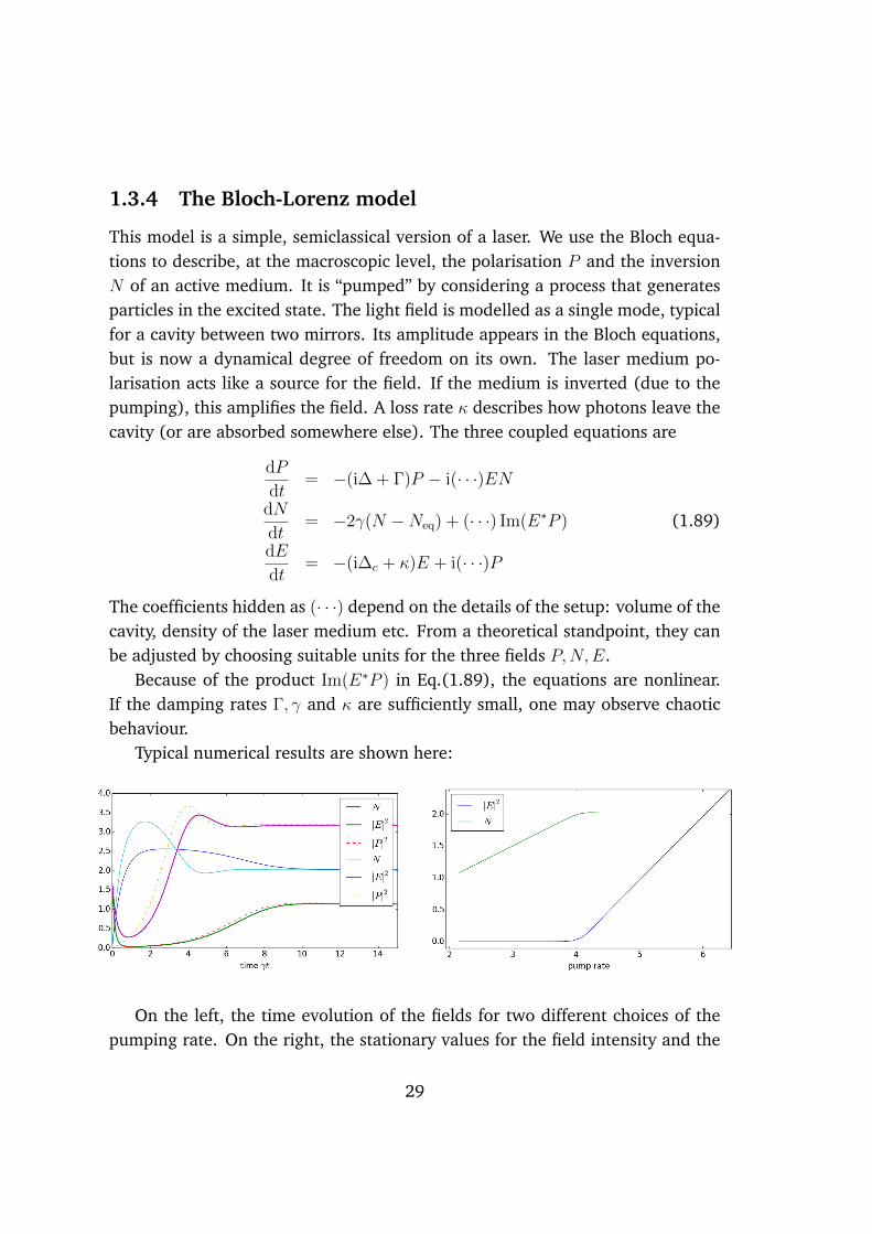
This model is a simple, semiclassical version of a laser. We use the Bloch equa-tions to describe, at the macroscopic level, the polarisation P and the inversionN of an active medium. It is “pumped” by considering a process that generatesparticles in the excited state. The light field is modelled as a single mode, typicalfor a cavity between two mirrors. Its amplitude appears in the Bloch equations,but is now a dynamical degree of freedom on its own. The laser medium po-larisation acts like a source for the field. If the medium is inverted (due to thepumping), this amplifies the field. A loss rate describes how photons leave thecavity (or are absorbed somewhere else). The three coupled equations are

dP

dt= �(i�+ �)P � i(· · ·)EN

dN

dt= �2�(N �Neq) + (· · ·) Im(E⇤

P ) (1.89)

dE

dt= �(i�c + )E + i(· · ·)P

The coefficients hidden as (· · ·) depend on the details of the setup: volume of thecavity, density of the laser medium etc. From a theoretical standpoint, they canbe adjusted by choosing suitable units for the three fields P,N,E.

Because of the product Im(E⇤P ) in Eq.(1.89), the equations are nonlinear.

If the damping rates �, � and are sufficiently small, one may observe chaoticbehaviour.

Typical numerical results are shown here:

On the left, the time evolution of the fields for two different choices of thepumping rate. On the right, the stationary values for the field intensity and the

29

inversion, as the pumping rate is changed. The relatively sharp change fromzero intensity to a linear dependence is called the laser threshold. Right at thethreshold, the amplification rate balances exactly the cavity loss rate . Belowthe threshold, the inversion is defined by the balance between pumping rate andthe radiative lifetime 1/�; for this reason, it increases linearly.

In the time evolution, one can see an initial stage of exponential growth forthe field intensity. This does not continue indefinitely because of a process calledsaturation: at high intensity, Rabi oscillations lead to an equilibration of thetwo populations, hence the inversion gets smaller. For strong (fast) interactionsbetween laser medium and light field, there is some “overshooting” and there issome damped oscillation before the system settles into its stationary state.

The stationary state of this system is an example of a “non-equilibrium steadystate” with a fixed “energy throughput”. The state is called non-equilibriumbecause it cannot be described by a temperature.

1.4 More notes on mixed states and dissipationThese notes go beyond the material covered in WS 19/20.

1.4.1 State of a two-level systemThis section contains details on a somewhat more axiomatic approach than what we did inthe lecture. You may jump directly to Eqs.(1.99, 1.100) that have been discussed in theProblem sessions.

The expectation values h�3i and h�i completely specify the state of the two-levelsystem.

Why is this so? A general observable is a hermitean 2 ⇥ 2 matrix. All thesematrices are linear combinations of Pauli matrices

A =

0

@ aee aeg

age agg

1

A =aee + agg

2+

aee � agg

2�3 + age� + aeg�

†

=aee + agg

2+X

j

aj�j, (1.90)

�1 = � + �† (1.91)

�2 = i(� � �†) (1.92)

30

with real coefficients aj.The above statement is true even for a more general definition of a state than

you may be used to. In the axiomatic language of quantum information, a stateis a mapping from a set of observables to their expectation values

⇢ : A 7! ⇢(A) = hAi⇢ (1.93)

Linear map with ⇢( ) = 1 (real or complex coefficients depending on choice ofobservable algebra) and ⇢(A) real for a hermitean A.

Now, the action of this map is determined by evaluation on basis vectors =Pauli matrices for a two-level system:

⇢(A) =aee + agg

2⇢( ) +

X

j

aj⇢(�j) =aee + agg

2⇢( ) +

X

j

ajsj (1.94)

with components of Bloch vector s = (s1, s2, s3).This definition is more general than complex linear combinations of |ei and

|gi. These states play a special role and are called pure states. They also corre-spond to special observables: projectors

� = |�ih�| (1.95)

This is also a hermitean operator with eigenvalues 0 or 1. A physical state hasthe property

⇢( �) � 0 for all |�i (1.96)

Physical interpretation: this is the probability of finding the system in the purestate |�i, which clearly must be a positive number.

Definition of density matrix (or density operator): any linear map on the vec-tor space of observables can be represented by a suitable linear form

⇢(A) = tr(⇢A) (1.97)

where ⇢ is a hermitean operator. This rule corresponds to the usual calculation ofexpectation values for mixed states in quantum statistics. In a finite-dimensionalsystem, it corresponds to the duality between linear forms and vectors: each lin-ear form can be represented as a scalar product with a suitable vector. This be-comes the Riesz representation theorem in an infinite-dimensional Hilbert space.

Using this for projector observables, we find from Eq.(1.96):

0 ⇢( �) = tr(⇢|�ih�|) = h�|⇢|�i (1.98)

31

Hence the diagonal elements of the density matrix are positive, in any basis. Thisconnects again to the interpretation of the probability of finding the system inthe state |�i.

Density operator as observable itself. Expectation value is called purity

Pu(⇢) = h⇢i⇢ = tr(⇢2) = . . . =1

2(1 + s

2) (1.99)

Calculation uses representation in terms of Bloch vector and Pauli matrices

⇢ =1

2

0

@ +X

j

sj�j

1

A =+ s · �

2(1.100)

How to generate mixed states

If a quantum system is closed and can be prepared in a pure state, then the time evolu-tion is simply Hamiltonian, | (t)i = U(t)| (0)i, and we don’t have to talk about quan-tum dissipation. This is not so in many settings, however.

There are a few examples how mixed (or non-pure) states arise.

(i) Initial mixed state. If the initial state is prepared within some probabilisticscheme, we have to work with an initial density matrix ⇢(0) 6= | (0)ih (0)|. This trans-lates our incomplete knowledge about the initial conditions. Recall that density matricescan be “mixed” by forming so-called convex linear combinations

⇢ = p⇢1 + q⇢2, p+ q = 1, p, q � 0, tr ⇢1,2 = 1 (1.101)

where the two density matrices ⇢1,2 are both normalized and p, q can be interpreted asprobabilities for preparing the two.

The time evolution is still simple if the system is closed (Hamiltonian evolution):

⇢(t) = U(t)⇢(0)U †(t) (1.102)

or in differential form (the von Neumann equation)

d

dt⇢ =

1

ih[H, ⇢] (1.103)

A typical example is an initial state prepared with a given temperature, ⇢(0) /

exp(�HI/T ). Interesting dynamics then happens only if HI 6= H.

Exercise. We actually don’t need to solve the von Neumann equation (1.103): byexpanding ⇢(0) in terms of its eigenvectors, we can just evolve these eigenvectors underSchrodinger’s equation and mix the final states. By linearity, the result is the same.

32

(ii) Reduced density matrix. The second example is that of a “system” S coupled toanother one, let’s call it “bath” or “environment” B. In this setting, we restrict ourselves(by construction) to observables that do not give any information about the state of theenvironment. These observables can be written in the form A⌦ B where B is the unitoperator in the environment’s Hilbert space. The key observation is that the expectationvalues for all system observables of this type can be calculated with the help of a densityoperator ⇢ for the system,

hA⌦ BiS+B = tr(A⇢S) (1.104)

Note that there are many authors who do not make the distinction between A⌦ B andA. The object ⇢S is called a reduced density operator (or matrix). It is sometimes written

⇢S = trB ⇢S+B = trB | S+Bih S+B| (1.105)

where the last writing assumes that system+environment are in a pure state | S+Bi.This procedure is called “taking the partial trace” over the environment (symbolic: trB),tracing out the environment, or “projecting into the system Hilbert space”. More precisely,the partial trace and the reduced density operator can be written in terms of the matrixelements (|ai, |bi are arbitrary system states)

ha|⇢S |bi =X

n

ha, n|⇢S+B|b, ni (1.106)

where the {|ni} form a complete basis for the environment. You will encounter some-times the writing

trB⇢S+B =X

n

hn|⇢S+B|ni (symbolic) (1.107)

where the object on the rhs has to be understood as having still the character of anoperator in the Hilbert space of the system.

The time evolution of a system coupled to an environment produces mixed states ina dynamical way:

⇢S(t) = trBhUS+B(t)⇢S+B(0)U

†S+B(t)

i(1.108)

even if ⇢S+B(0) starts off in a pure state. This is called the “Nakajima-Zwanziger” projec-tion. This construction is, of course, only relevant if (i) the initial state is not factorized(it is entangled) or (ii) there is some interaction between S and B. Otherwise US+B(t)

factorizes, and the partial trace simply reduces to

trB(US ⌦ UB)(⇢S ⌦ ⇢B)(US ⌦ UB)†

= trB(US⇢SU†S)⌦ (UB⇢BU

†B)

= US⇢SU†S trB(UB⇢BU

†B)

= US⇢SU†S (1.109)

33

The Nakajima-Zwanziger projection (1.108) shares many physically interesting featuresand is at the basis of many generalizations of the Schrodinger equation to “open quan-tum systems”. The system+environment setting thus provides a conceptual frameworkto introduce dissipation into quantum mechanics. We shall use it in the later parts of thequantum optics course.

(iii) Measure and forget. This procedure of mixing states is related to the sys-tem+environment setting, but it arises from the basic postulates and can be formulatedwithout introducing explicitly an environment. We recall the standard rule (von Neu-mann and Luders) of what happens to a quantum state when an observable A has beenmeasured (with eigenvalue a):

| i 7! |ai (1.110)

The system has “collapsed” to an eigenstate |ai of the observable. This is still a purestate and corresponds to a “perfect” or projective measurement.

Now introduce probabilities and forgetting. The probability that we get the eigen-value a is, of course, given by p(a) = |ha| i|

2 = tr (|aiha|⇢) where ⇢ = | ih | for aninitially pure state. Hence if we start off with a non-pure state, the von-Neumann-Ludersrule reads

⇢ 7! |aiha| (1.111)

In this way, we can even “purify” a mixed state! After all, the states in quantum mechan-ics just reflect the knowledge we have about the system.

The perfect measurement is often quite difficult to perform, however, and manystates can be found that are still compatible with the measured eigenvalue a. In otherwords, our measurement cannot distinguish precisely among the different eigenstates|ai. This is the typical scenario if the eigenvalues are continuously distributed.

Now let us imagine that we only know that we have performed the measurement “Isthe system in state |ai?”, but have forgotten the result. We know that with probabilityp(a), the state has collapsed (projective measurement). But with probability 1 � p(a),something else has happened. Let us assume that the state remained unchanged. Byforgetting the result of the measurement, we are forced to assign to the system a mixedstate:

⇢ 7! (1� p(a))⇢+ p(a)|aiha| (simplest approximation) (1.112)

This scenario is called an “imperfect” or weak measurement. If the probability p(a) issmall, the state change is also small. This is the scenario we shall use to motivate thedissipative evolution of a two-level system. An alternative notation for the probabilistic

34

mixture of the two states can be given

⇢ 7!

(⇢ with prob 1� p(a)

|aiha| with prob p(a)(1.113)

Remark. We can re-phrase this procedure within a system+environment setting. Suppose thatwe couple the system to an environment that can “measure” whether the system is in state |ai.After some evolution time, we get an entangled state (| i is the initial system density state,assumed pure and |0i the initial environment state)

| , 0i 7! ha| i|a, 1ai+ US+B | ?, 0i

where |1ai is the (“conditional”) environment state and | ?i is the (non-normalized) systemstate orthogonal to |ai. We construct the reduced density operator and get a mapping (betweensystem operators)

| ih | 7! trB(ha| i|a, 1ai+ US+B | ?, 0i)(ha| i|a, 1ai+ US+B | ?, 0i)†

Now comes the key assumption: the coupling to the environment has been sufficiently strong sothat one can distinguish the environment states |1ai, |0i, and the environment states containedin US+B | ?, 0i. The best we can do is that these states are orthogonal

h1a|0i ⇡ 0, trB US+B | ?, 0iha, 1a| ⇡ 0 (1.114)

This removes the mixed (crossed) terms in the partial trace, and we get a mixture (with p(a) =

|ha| i|2 as in QM I)

| ih | 7! |aiha|p(a) + trB US+B | ?, 0ih ?, 0|U†S+B

where the first term contains the projection onto the eigenstate. The simplest assumption forthe second term is that the environment does not evolve at all, provided the system is in theorthogonal state | ?i. Then US+B | ?, 0i ⇡ | ?, 0i, and the partial trace gives

| ih | 7! |aiha|p(a) + ?| ih | ?

where ? projects into the subspace orthogonal to |ai. The last term has a trace 1 � p(a), as inEq.(1.112), but differs slightly because of the projection. We come back to this when discussingspontaneous emission.

See the introductory article “Decoherence and the transition from quantum to classical” byZurek (1991) for more details on this discussion. The main message is that the coupling to anenvironment can provide the same physics as measuring a quantum system.

1.4.2 Quantum jump approach for a two-level systemMaterial not covered in WS 19/20.

35

Evolution over time step �t. “Sufficiently small” in some sense to put together Hamil-tonian evolution and measurement (“monitoring”) by an environment.

Pure Hamiltonian (for simplicity, time-independent, applies in rotating frame) (h =

1)

⇢(t+�t) ⇡ ( � iH�t)⇢(t)( + iH�t) = ⇢(t)� i [H�t, ⇢(t)] +O(�t2) (1.115)

Now observing and forgetting about the results. We consider two scenarios.

Dephasing: measuring energy states. We assume that with a probability �p, wehave been able to determine in which energy eigenstate the two-level system is. Thiscan be achieved, for example, by performing measurements on the environment. Therule for “measure and forget” then gives (we have three outcomes)

⇢(t+�t) =

8>><

>>:

⇢(t) with prob 1��p

|gihg| with prob �p ⇢gg(t)

|eihe| with prob �p ⇢ee(t)

(1.116)

This gives the mixed state, as a simple calculation shows

⇢(t+�t) = (1��p)⇢(t) +�p

X

a=g, e

ha|⇢(t)|ai |aiha|

= (1� 1

2�p)⇢(t) + 1

2�p�3⇢(t)�3 (1.117)

Concatenate the two elementary processes (1.115, 1.117) and construct an approxi-mate time derivative

�⇢

�t⇡ �i [H, ⇢(t)] +

�p

2�t{�3⇢(t)�3 � ⇢(t)} (1.118)

This is the dynamical equation for a system subject to dephasing. The equation is inthe so-called Lindblad form (see Eq.(1.126)), a general form for the time evolution ofan open system that we shall derive later in the lecture. The rate �p/2�t is called the“dephasing rate”.

Exercise. Switch to the Heisenberg picture and calculate from Eq.(1.118) the rate ofchange h��/�ti of the Bloch vector. Show that the non-Hamiltonian terms give

h��i

�t

����non�H

⇡ ��p

2�th�i (1.119)

while h��3/�ti = 0. The monitoring of the energy levels thus does not change theinversion which is not surprising, since we made the assumption that the measured

36

eigenstate is not changed. The dipole, that captures the relative phase of superpositionstates in the energy basis, however, decays with a rate �p/2�t. We can thus interpret thedipole relaxation rate as the rate at which the environment acquires information aboutthe system’s energy. Note also that the decay of the dipole is the price to pay for themeasurement in the energy basis – the quantum-mechanical rule that “any measurementperturbs the system” still holds.

Spontaneous emission: quantum jumps. The second scenario is based on theobservation of the photons that a two-level atom can emit. We assume that over theevolution time �t, the probability to detect an emitted photon is �p ⇢ee(t). We haveclearly �p = ��t according to the law of radioactive decay. In addition, once thisphoton has been detected, we know that the atom must be in the ground state |gi. Thisfeature is different from the previous scenario where the measurement perturbed thesystem in a weaker way.

Now imagine that we throw away the information that a photon has been emitted.The state then mixes into

⇢(t+�t) =

(⇢0 with prob 1��p

|gihg| with prob �p ⇢ee(t)(1.120)

where the state ⇢0 is normalized and corresponds to the event “no photon detected”.

This can be translated into

⇢(t+�t) = ⇢00 +�p ⇢ee(t) |gihg| = ⇢

00 +�p�⇢(t)�† (1.121)

where ⇢00 is a non-normalized state with trace 1��p ⇢ee(t). The second term appearinghere is called a “quantum jump”: the photon emission happens when the atom jumpsfrom the excited to the ground state |ei ! |gi. The ladder (or annihilation) operator �plays here a very intuitive role. If ⇢(t) = | (t)ih (t)| is a pure state, the system jumps tothe state �| (t) at the photon emission.

The first term ⇢00 in Eq.(1.121) now takes care of the conservation of probabilities.

In our first guess (1.112) we simply took ⇢00 = (1��p ⇢ee)⇢. This recipe must be refinedhere, for two reasons.

One reason is more formal: we want that ⇢(t + �t) to be expressed as a linearmap of the state ⇢(t), but �p ⇢ee ⇢ is quadratic in ⇢. This reason is deeply rooted inthe linearity of quantum mechanics. The Nakajima-Zwanziger scheme (1.108) whichprovides a very general framework for quantum dissipation, is also a linear map betweendensity matrices.

The second reason is that the event “no photon has been detected” actually changesour knowledge about the system. Qualitatively speaking, it increases our confidence that

37

the system might be in the ground state. We are having less the tendency to think it is inthe excited state. After all, if the system is in the excited state, we would expect at somepoint a photon to appear! In the opposite limit, if over a very long time we do not detectany photons, the system must be (with a very high probability) in the ground state, andwe have gained this knowledge from the sequence of “no-photon” events.

We are thus led to the following refined approximation

⇢00

⇡

⇣�

1

2�p |eihe|

⌘⇢(t)

⇣�

1

2�p |eihe|

⌘

⇡ ⇢(t)� 1

2�p

n�†� ⇢(t) + ⇢(t)�†�

o(1.122)

Putting Eqs.(1.121, 1.122), together, we find the so-called “master equation” for a two-level system with spontaneous decay

�⇢

�t⇡ �i [H, ⇢(t)] +

�p

�t

n�⇢(t)�† � 1

2�†�⇢(t)� 1

2⇢(t)�†�

o(1.123)

More details on this derivation can be found in the paper by Dalibard & al. (1992) on a“Wave-Function Approach to Dissipative Processes in Quantum Optics”.

Exercise. By working out matrix elements of this equation, identify � = �p/�t withthe spontaneous decay rate. The important message of this equation is that spontaneousemission changes both the inversion and the dipole:

h��i

�t

����non�H

⇡ �1

2�h�i (1.124)

h��3i

�t

����non�H

⇡ ��(h�3i+ 1) (1.125)

1.4.3 Lindblad master equation

Without going into the details of the derivation, we just state here that the gen-eralized von-Neumann equations (1.118, 1.123) are special cases of a generaltheorem about the time evolution of a quantum system, the

Lindblad theorem. If a time evolution Tt : ⇢(0) 7! ⇢(t) satisfies the followingconditions:

– the map Tt is linear and maps density matrices onto density matrices;

38

– the map Tt is completely positive3;

– expectation values evolve continuous in time;

– repeating the map corresponds to adding time lapses, TtTt0 = Tt+t0 ,

then there exists a hermitean operator H and a countable set of system operatorsLk (k = 1 . . . K) such that the state ⇢(t) = Tt⇢(0) solves the differential equation

d⇢

dt= �i [H, ⇢] +

KX

k=1

nLk⇢L

†k �

1

2L†kLk⇢�

1

2⇢L

†kLk

o(1.126)

The operators Lk are called Lindblad or jump operators.For spontaneous emission and dephasing, only a single Lindblad operator

appears, as shown in this Table:

spont. decay dephasingLindblad operator p

� �

q/2 �3

where is the dephasing rate. Keeping both Lindblad operators in the timeevolution, gives the Bloch equations (1.79, 1.80) with a dephasing rate � =

+ �/2. The Lindblad theorem is proven later on in the quantum optics lecture.A simple proof can be found in Nielsen & Chuang (2011) and Henkel (2007).

1.5 Spin language and Bloch sphere

1.5.1 Bloch vector

Bloch vector: expectation value of Pauli matrices

s(t) = h (t)|�| (t)i (1.127)

Typical states, described by analogy to points on a sphere (spherical coordi-nates):

• ground state = south pole3Qualitatively speaking: density matrices are mapped onto density matrices even if the system

is augmented by some environment and the map Tt augmented by “nothing happens with theenvironment”.

39

• excited state = north pole

• superposition with equal weights (|ei+ei'|gi)/p2 = a point on the equator

with longitude '

Translation into macroscopic observables: occupations (s3) and polarization(s1, s2).

1.5.2 Bloch dynamics

Dissipative dynamics for components of Bloch vector, contains the following pro-cesses:

Spontaneous decay rate � (time scale called T1 in spin resonance).Decoherence or dephasing rate � (coherence time T2).Set of Bloch equations (assuming that ⌦ is real)

ds1dt

= �s2 � �s1

ds2dt

= ��s1 � ⌦s3 � �s2

ds3dt

= ⌦s2 � �(s3 + 1) (1.128)

in rotating frame at ! = !L, detuning � = !L � !A, Rabi frequency ⌦ ⇠ EL.Geometric moves:

– rotation (from Hamiltonian, axis defined by detuning � and Rabi frequency ⌦)– contraction (from decoherence rate � and decay rate �), squeezes sphere into‘lemon’ with axis in the ‘north-south’ direction– displacement towards the south pole (ground state), from the decay rate �

Solution to time-dependent Schrodinger equation: Rabi oscillations,Sec.1.2.4.

40

Rabi oscillations with nonzero detuning: populations of the two lev-els, pe(t) and pg(t), vs. time.

‘Absorption spectrum’ = amplitude of Rabi oscillations in pe(t) vs.laser frequency. Lorentz = name for the line shape = dependence ondetuning � = !L � !A. � = ‘natural linewidth’ = minimal width ofthe spectrum when the Rabi frequency ⌦ becomes small.

41

Sketch for rotation axis n of the spin vector representing the state ofthe atom. Initial states ~g = ground state (‘spin down’), ~e = excitedstate (‘spin up’). The angle ✓, proportional to the Rabi frequency,gives the opening angle of a cone on which the spin vector rotates.

Rotation axis for a laser field on resonance: the spin vector rotates‘full circle’ from spin down to spin up and back. Geometric represen-tation of Rabi oscillations (on resonance, � = 0).

General Hamiltonian is decomposed into unit matrix and Pauli matrices

H = H0 +X

j

Hj�j (1.129)

This gives the ‘coherent dynamics’

@s

@t=

2

hH⇥ s (1.130)

42

= rotation of the Bloch vector. By analogy to the precession of a spin in a mag-netic field, one calls the components Hj in Eq.(1.129) the ‘effective magneticfield’.

Rotations preserve the length of a vector: if one starts with a Bloch vector onthe surface of the sphere, it will remain there if the time evolution is coherent(purely Hamiltonian). The length of the Bloch vector is not preserved by dissi-pative processes: they push the state into the interior of the Bloch sphere where‘incoherent states’ occur (see Sec.??).

1.6 Outlook: light-matter interaction

The description of atom+light interaction that we have developed so far, com-plemented by techniques to quantize the field (see following chapter) is the basisfor most of the phenomena that have been studied in the quantum optics of two-level system. One can discuss the following topics (we give a selection in thislecture):

• Rabi oscillations in a classical monochromatic field;

• spontaneous decay of an excited atom into the continuum of vacuum fieldmodes (initially in the ground state);

• interaction of light with a medium of two-level atoms. One has to re-interpret the density matrix as giving the state of a macroscopic numberof atoms. The occupations pe, pg, for example, then are proportional tothe number of atoms (or molecules) in the excited and ground state. Theatomic dipole becomes, after multiplication with the atom density, thepolarization field (electric dipole moment per volume). Coupled to theMaxwell equations where this polarization field enters as a source term,one then has a simple “semiclassical” description for a laser, for a solar cell,for a semi-conductor. The Bloch equations in this case may contain morecomplicated terms.

• collapse and revival of Rabi oscillations when the atom couples to a singlequantized field mode. The collapse and the revival occurs because theRabi frequency depends on the photon number, and the oscillations for

43

the different Fock state components of a field state (a coherent state, forexample) get out of phase;

• resonance fluorescence is the radiation emitted by an atom driven by anear-resonant laser field. This combines Rabi oscillations in a classicalfield with the emission of photons into the empty mode continuum. Ofparticular interest is the spectrum of this emission: it contains, for suf-ficiently strong driving, two sidebands, split by the Rabi frequency fromthe central line (centered at the laser frequency). The central line con-tains a monochromatic component (‘elastic scattering’, related to the laser-induced dipole moment as in classical electrodynamics) and a broadenedcomponent of Lorentzian shape, related to spontaneous emission. Thisspectrum is a cornerstone of quantum optics and one of the few examplesof a non-perturbative calculation in quantum electrodynamics.

There are also physical effects which cannot be captured by our two-leveldescription. They are related to the failure of the resonance approximation:

• the Lamb shift, a displacement of certain energy levels in atoms, arisesfrom a very wide frequency continuum of vacuum field modes. One doesget a wrong result if in the atom+field interaction, non-resonant processesare neglected.

• for short light pulses (roughly in the 1 fs range), one needs more than twoenergy levels, and even continuum states may be necessary for an accuratedescription. These pulses can generate ‘high harmonics’ as an electron ispulled away from the atomic core and pushed back under the influence ofso-called ‘few-cycle pulses’ which can be very intense (electric fields com-parable to those in the atom itself, Rabi frequencies comparable to atomicBohr frequencies).

Bibliography

C. Cohen-Tannoudji, J. Dupont-Roc & G. Grynberg (1987). Photons et atomes — Introduc-tion a l’electrodynamique quantique. InterEditions, Paris. English translation: Photonsand Atoms — Introduction to Quantum Electrodynamics (Wiley, New York 1989).

44

D. P. Craig & T. Thirunamachandran (1984). Molecular Quantum Electrodynamics. Aca-demic Press, London.

J. Dalibard, Y. Castin & K. Mølmer (1992). Wave-Function Approach to DissipativeProcesses in Quantum Optics, Phys. Rev. Lett. 68, 580–83. Postprint arXiv:0805.4002.

P. A. M. Dirac (1927). The Quantum Theory of the Emission and Absorption of Radiation,Proc. Roy. Soc. (London) A 114, 243–65.

H. Haken & H. C. Wolf (2000). The Physics of Atoms and Quanta. Advanced Texts inPhysics. Springer, Heidelberg Berlin, 6th edition.

C. Henkel (2007). Laser theory in manifest Lindblad form, J. Phys. B 40, 2359–71.

C. Itzykson & J. B. Zuber (2006). Quantum field theory. Dover, New York.

M. A. Nielsen & I. L. Chuang (2011). Quantum Computation and Quantum Information.Cambridge University Press, Cambridge, 2nd edition.

W. H. Zurek (1991). Decoherence and the transition from quantum to classical, PhysicsToday 44 (10), 36–44. Update: quant-ph/0306072.

45