QUANTUM MECHANICS • Introduction : Quantum Mechanics with ...
Introduction to Quantum Mechanics
From Geometry to Spectra
John F. Lindner
Physics Department
The College of Wooster
2015 January 4

2

Contents
List of Tables 7
List of Figures 9
1 Quantum Phenomenology 111.1 Preamble: Sorting Photons . . . . . . . . . . . . . . . . . . . . . 111.2 Interference & Superposition . . . . . . . . . . . . . . . . . . . . 13
1.2.1 Beam Splitter Probabilities . . . . . . . . . . . . . . . . . 141.2.2 Two Interpretations . . . . . . . . . . . . . . . . . . . . . 151.2.3 Mach-Zehnder Interferometer . . . . . . . . . . . . . . . . 161.2.4 Quantum Eraser . . . . . . . . . . . . . . . . . . . . . . . 181.2.5 Interaction-Free Measurement . . . . . . . . . . . . . . . . 191.2.6 Quantum Computing . . . . . . . . . . . . . . . . . . . . 201.2.7 Mach-Zehnder Classical Model . . . . . . . . . . . . . . . 211.2.8 Mach-Zehnder Quantum Model 1 . . . . . . . . . . . . . . 221.2.9 Mach-Zehnder Quantum Model 2 . . . . . . . . . . . . . . 22
1.3 Measurement & Entanglement . . . . . . . . . . . . . . . . . . . 251.3.1 Hilbert Space Preview . . . . . . . . . . . . . . . . . . . . 251.3.2 Quantum Evolution . . . . . . . . . . . . . . . . . . . . . 251.3.3 Schrodinger’s Cat and the Measurement Problem . . . . . 261.3.4 Polarization . . . . . . . . . . . . . . . . . . . . . . . . . . 271.3.5 Crossed Polarizers . . . . . . . . . . . . . . . . . . . . . . 281.3.6 Entangled States . . . . . . . . . . . . . . . . . . . . . . . 301.3.7 EPR-Bohm Experiment . . . . . . . . . . . . . . . . . . . 311.3.8 Bell’s Inequality . . . . . . . . . . . . . . . . . . . . . . . 32
Problems . . . . . . . . . . . . . . . . . . . . . . . . . . . . . . . . . 34
2 Hilbert Spaces 392.1 Euclidean Space . . . . . . . . . . . . . . . . . . . . . . . . . . . 392.2 Generic Hilbert Space . . . . . . . . . . . . . . . . . . . . . . . . 40
2.2.1 Vectors . . . . . . . . . . . . . . . . . . . . . . . . . . . . 402.2.2 Operators . . . . . . . . . . . . . . . . . . . . . . . . . . . 412.2.3 Dual Space . . . . . . . . . . . . . . . . . . . . . . . . . . 412.2.4 Hermitian Operators . . . . . . . . . . . . . . . . . . . . . 42
3

Contents 4
2.2.5 Unitary Operators . . . . . . . . . . . . . . . . . . . . . . 432.3 Matrix Representations . . . . . . . . . . . . . . . . . . . . . . . 442.4 Uncountable Hilbert Spaces . . . . . . . . . . . . . . . . . . . . . 452.5 Quantum Example . . . . . . . . . . . . . . . . . . . . . . . . . . 462.6 Commutation . . . . . . . . . . . . . . . . . . . . . . . . . . . . . 48Problems . . . . . . . . . . . . . . . . . . . . . . . . . . . . . . . . . 50
3 Symmetry Commutators 533.1 Spacetime Symmetries . . . . . . . . . . . . . . . . . . . . . . . . 533.2 Spacetime Closures . . . . . . . . . . . . . . . . . . . . . . . . . . 553.3 State Space Symmetry Generators . . . . . . . . . . . . . . . . . 61
3.3.1 Generic Commutator . . . . . . . . . . . . . . . . . . . . . 613.3.2 Commutator Antisymmetries . . . . . . . . . . . . . . . . 623.3.3 Phase Constants . . . . . . . . . . . . . . . . . . . . . . . 63
Problems . . . . . . . . . . . . . . . . . . . . . . . . . . . . . . . . . 67
4 Dynamics Commutators 694.1 Position Operator . . . . . . . . . . . . . . . . . . . . . . . . . . . 69
4.1.1 Position and Space Translations . . . . . . . . . . . . . . 704.1.2 Position and Rotations . . . . . . . . . . . . . . . . . . . . 714.1.3 Position and Boosts . . . . . . . . . . . . . . . . . . . . . 724.1.4 Position and Time Translations . . . . . . . . . . . . . . . 74
4.2 Velocity Operator . . . . . . . . . . . . . . . . . . . . . . . . . . . 744.3 Symmetry Generators Dynamical Identities . . . . . . . . . . . . 76
4.3.1 Free Particle Without Spin . . . . . . . . . . . . . . . . . 764.3.2 Interacting Particles Without Spin . . . . . . . . . . . . . 814.3.3 Free Particle With Spin . . . . . . . . . . . . . . . . . . . 82
4.4 Position Space Schrodinger Equation . . . . . . . . . . . . . . . . 83Problems . . . . . . . . . . . . . . . . . . . . . . . . . . . . . . . . . 85
5 Harmonic Oscillator 875.1 Classical Harmonic Oscillator . . . . . . . . . . . . . . . . . . . . 875.2 Commutator Solution . . . . . . . . . . . . . . . . . . . . . . . . 88
5.2.1 Dimensionless Variables . . . . . . . . . . . . . . . . . . . 885.2.2 Creation & Annihilation Operators . . . . . . . . . . . . . 895.2.3 Number Operator Spectrum . . . . . . . . . . . . . . . . . 895.2.4 Energy Spectrum . . . . . . . . . . . . . . . . . . . . . . . 915.2.5 Wave Functions . . . . . . . . . . . . . . . . . . . . . . . . 91
5.3 Differential Equation Solution . . . . . . . . . . . . . . . . . . . . 925.3.1 Dimensionless Variables . . . . . . . . . . . . . . . . . . . 935.3.2 Asymptotic Behavior . . . . . . . . . . . . . . . . . . . . . 935.3.3 Power Series Solution . . . . . . . . . . . . . . . . . . . . 945.3.4 Power Series Diverges . . . . . . . . . . . . . . . . . . . . 955.3.5 Truncate Series . . . . . . . . . . . . . . . . . . . . . . . . 955.3.6 Standard Form Solutions . . . . . . . . . . . . . . . . . . 965.3.7 Classical Correspondence . . . . . . . . . . . . . . . . . . 97
Contents 5
5.4 Angular Momentum . . . . . . . . . . . . . . . . . . . . . . . . . 985.5 Two-Dimensional Harmonic Oscillator . . . . . . . . . . . . . . . 101
5.5.1 Classical Case . . . . . . . . . . . . . . . . . . . . . . . . . 1015.5.2 Eigenstates of Energy . . . . . . . . . . . . . . . . . . . . 1015.5.3 Eigenstates of Energy & Angular Momentum . . . . . . . 103
Problems . . . . . . . . . . . . . . . . . . . . . . . . . . . . . . . . . 106
6 Hydrogen Atom 1076.1 Classical Kepler Problem . . . . . . . . . . . . . . . . . . . . . . 1076.2 Quantum Kepler Problem . . . . . . . . . . . . . . . . . . . . . . 108
6.2.1 Angular Momentum . . . . . . . . . . . . . . . . . . . . . 1086.2.2 Eccentricity . . . . . . . . . . . . . . . . . . . . . . . . . . 1096.2.3 Hamiltonian . . . . . . . . . . . . . . . . . . . . . . . . . . 1116.2.4 Eigenvalues . . . . . . . . . . . . . . . . . . . . . . . . . . 112
Problems . . . . . . . . . . . . . . . . . . . . . . . . . . . . . . . . . 114
Appendices
A Notation 115
B Bibliography 117

Contents 6

List of Tables
2.1 Bra ket Matrices . . . . . . . . . . . . . . . . . . . . . . . . . . . 452.2 Bases Comparison . . . . . . . . . . . . . . . . . . . . . . . . . . 46
3.1 Spacetime closure . . . . . . . . . . . . . . . . . . . . . . . . . . . 613.2 Generator Commutators with Phase Constants . . . . . . . . . . 633.3 Generator Commutators . . . . . . . . . . . . . . . . . . . . . . . 66
4.1 Mixed Commutators . . . . . . . . . . . . . . . . . . . . . . . . . 764.2 Transformation Table . . . . . . . . . . . . . . . . . . . . . . . . 764.3 Dynamical Commutators . . . . . . . . . . . . . . . . . . . . . . 81
5.1 First few harmonic oscillator eigenvalues and eigenfunctions. . . . 96
6.1 Kepler Commutators . . . . . . . . . . . . . . . . . . . . . . . . . 108
A.1 Symbols . . . . . . . . . . . . . . . . . . . . . . . . . . . . . . . . 115
7

List of Tables 8
List of Figures
1.1 Calcite crystal . . . . . . . . . . . . . . . . . . . . . . . . . . . . 111.2 Polarization sorters . . . . . . . . . . . . . . . . . . . . . . . . . . 121.3 Photon and a ⊕ sorter . . . . . . . . . . . . . . . . . . . . . . . . 131.4 Photon and a ⊕ sorter & antisorter . . . . . . . . . . . . . . . . . 131.5 Beam splitter . . . . . . . . . . . . . . . . . . . . . . . . . . . . . 141.6 Beam splitter & single photons . . . . . . . . . . . . . . . . . . . 151.7 Mach-Zehnder interferometer . . . . . . . . . . . . . . . . . . . . 161.8 Mach-Zehnder interferometer & single photons . . . . . . . . . . 171.9 Quantum eraser . . . . . . . . . . . . . . . . . . . . . . . . . . . . 181.10 Interaction-free measurement . . . . . . . . . . . . . . . . . . . . 191.11 Quantum computing . . . . . . . . . . . . . . . . . . . . . . . . . 201.12 Rotating arrow . . . . . . . . . . . . . . . . . . . . . . . . . . . . 221.13 Rotating arrow & single photons . . . . . . . . . . . . . . . . . . 231.14 Photon interferometer states . . . . . . . . . . . . . . . . . . . . 241.15 Schrodinger cat states . . . . . . . . . . . . . . . . . . . . . . . . 271.16 Linear polarizer . . . . . . . . . . . . . . . . . . . . . . . . . . . . 291.17 Crossed polarizers & single photons . . . . . . . . . . . . . . . . . 301.18 Decay of positronium . . . . . . . . . . . . . . . . . . . . . . . . . 311.19 EPR-Bohm experiment . . . . . . . . . . . . . . . . . . . . . . . 32
2.1 Cantor’s diagonal arguments . . . . . . . . . . . . . . . . . . . . 45
3.1 Boosts . . . . . . . . . . . . . . . . . . . . . . . . . . . . . . . . . 553.2 Finite rotations . . . . . . . . . . . . . . . . . . . . . . . . . . . . 553.3 Spacetime gaps . . . . . . . . . . . . . . . . . . . . . . . . . . . . 60
4.1 Translated Function . . . . . . . . . . . . . . . . . . . . . . . . . 694.2 Infinitesimal rotation . . . . . . . . . . . . . . . . . . . . . . . . . 71
5.1 Oscillator eigenfunctions . . . . . . . . . . . . . . . . . . . . . . . 975.2 Oscillator classical correspondence . . . . . . . . . . . . . . . . . 985.3 Angular Momentum Quantum Numbers . . . . . . . . . . . . . . 101
9

List of Figures 10
Chapter 1
Quantum Phenomenology
Of the two great physics revolutions of the early 1900s, relativity “completes”classical physics, but quantum physics subsumes it.
Richard Feynman wrote, “Things on a very small scale behave like nothingthat you have any direct experience about. They do not behave like waves, theydo not behave like particles, they do not behave like clouds, or billiard balls, orweights on springs, or like anything that you have ever seen”[1].
One can’t learn about atoms by playing with billiard balls, but one can learnabout billiard balls by studying atoms. Classical physics follows from quantumphysics, not the other way around.
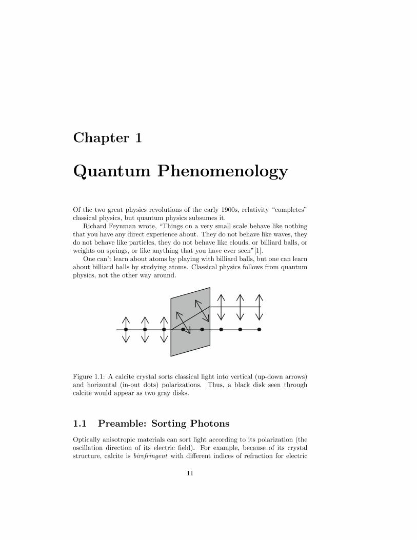
Figure 1.1: A calcite crystal sorts classical light into vertical (up-down arrows)and horizontal (in-out dots) polarizations. Thus, a black disk seen throughcalcite would appear as two gray disks.
1.1 Preamble: Sorting Photons
Optically anisotropic materials can sort light according to its polarization (theoscillation direction of its electric field). For example, because of its crystalstructure, calcite is birefringent with different indices of refraction for electric
11
Chapter 1. Quantum Phenomenology 12
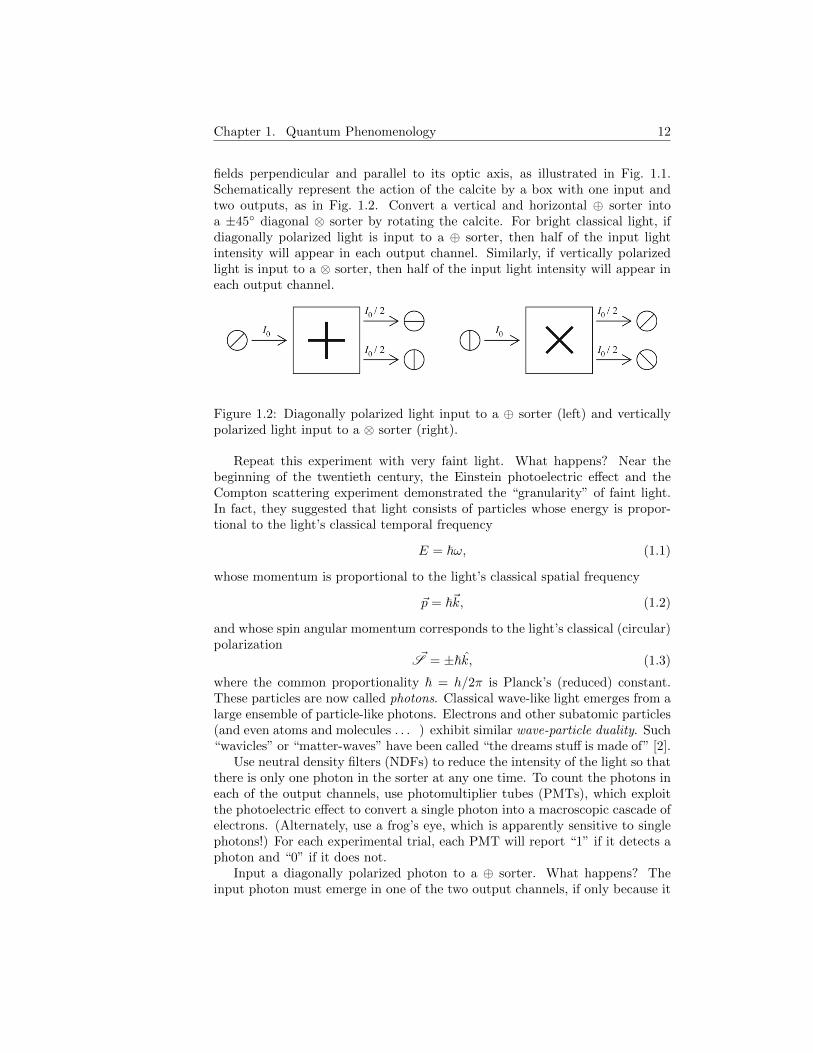
fields perpendicular and parallel to its optic axis, as illustrated in Fig. 1.1.Schematically represent the action of the calcite by a box with one input andtwo outputs, as in Fig. 1.2. Convert a vertical and horizontal ⊕ sorter intoa ±45◦ diagonal ⊗ sorter by rotating the calcite. For bright classical light, ifdiagonally polarized light is input to a ⊕ sorter, then half of the input lightintensity will appear in each output channel. Similarly, if vertically polarizedlight is input to a ⊗ sorter, then half of the input light intensity will appear ineach output channel.
Figure 1.2: Diagonally polarized light input to a ⊕ sorter (left) and verticallypolarized light input to a ⊗ sorter (right).
Repeat this experiment with very faint light. What happens? Near thebeginning of the twentieth century, the Einstein photoelectric effect and theCompton scattering experiment demonstrated the “granularity” of faint light.In fact, they suggested that light consists of particles whose energy is propor-tional to the light’s classical temporal frequency
E = ~ω, (1.1)
whose momentum is proportional to the light’s classical spatial frequency
~p = ~~k, (1.2)
and whose spin angular momentum corresponds to the light’s classical (circular)polarization
~S = ±~k, (1.3)
where the common proportionality ~ = h/2π is Planck’s (reduced) constant.These particles are now called photons. Classical wave-like light emerges from alarge ensemble of particle-like photons. Electrons and other subatomic particles(and even atoms and molecules . . . ) exhibit similar wave-particle duality. Such“wavicles” or “matter-waves” have been called “the dreams stuff is made of” [2].
Use neutral density filters (NDFs) to reduce the intensity of the light so thatthere is only one photon in the sorter at any one time. To count the photons ineach of the output channels, use photomultiplier tubes (PMTs), which exploitthe photoelectric effect to convert a single photon into a macroscopic cascade ofelectrons. (Alternately, use a frog’s eye, which is apparently sensitive to singlephotons!) For each experimental trial, each PMT will report “1” if it detects aphoton and “0” if it does not.
Input a diagonally polarized photon to a ⊕ sorter. What happens? Theinput photon must emerge in one of the two output channels, if only because it
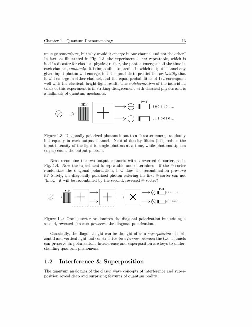
Chapter 1. Quantum Phenomenology 13
must go somewhere, but why would it emerge in one channel and not the other?In fact, as illustrated in Fig. 1.3, the experiment is not repeatable, which isitself a disaster for classical physics; rather, the photon emerges half the time ineach channel, randomly. It is impossible to predict in which output channel anygiven input photon will emerge, but it is possible to predict the probability thatit will emerge in either channel, and the equal probabilities of 1/2 correspondwell with the classical, bright-light result. The indeterminism of the individualtrials of this experiment is in striking disagreement with classical physics and isa hallmark of quantum mechanics.
Figure 1.3: Diagonally polarized photons input to a ⊕ sorter emerge randomlybut equally in each output channel. Neutral density filters (left) reduce theinput intensity of the light to single photons at a time, while photomultipliers(right) count the output photons.
Next recombine the two output channels with a reversed ⊕ sorter, as inFig. 1.4. Now the experiment is repeatable and determined! If the ⊕ sorterrandomizes the diagonal polarization, how does the recombination preserveit? Surely, the diagonally polarized photon entering the first ⊕ sorter can not“know” it will be recombined by the second, reversed ⊕ sorter?
Figure 1.4: One ⊕ sorter randomizes the diagonal polarization but adding asecond, reversed ⊕ sorter preserves the diagonal polarization.
Classically, the diagonal light can be thought of as a superposition of hori-zontal and vertical light and constructive interference between the two channelscan preserve its polarization. Interference and superposition are keys to under-standing quantum phenomena.
1.2 Interference & Superposition
The quantum analogues of the classic wave concepts of interference and super-position reveal deep and surprising features of quantum reality.
Chapter 1. Quantum Phenomenology 14
1.2.1 Beam Splitter Probabilities
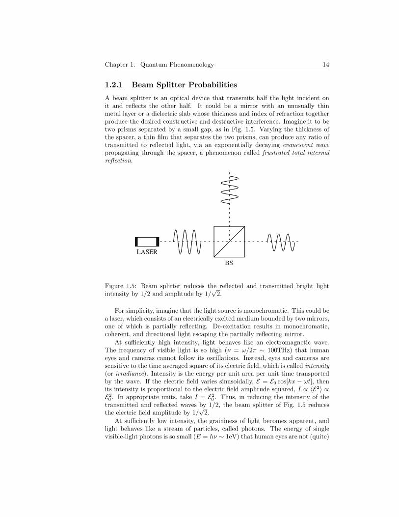
A beam splitter is an optical device that transmits half the light incident onit and reflects the other half. It could be a mirror with an unusually thinmetal layer or a dielectric slab whose thickness and index of refraction togetherproduce the desired constructive and destructive interference. Imagine it to betwo prisms separated by a small gap, as in Fig. 1.5. Varying the thickness ofthe spacer, a thin film that separates the two prisms, can produce any ratio oftransmitted to reflected light, via an exponentially decaying evanescent wavepropagating through the spacer, a phenomenon called frustrated total internalreflection.
Figure 1.5: Beam splitter reduces the reflected and transmitted bright lightintensity by 1/2 and amplitude by 1/
√2.
For simplicity, imagine that the light source is monochromatic. This could bea laser, which consists of an electrically excited medium bounded by two mirrors,one of which is partially reflecting. De-excitation results in monochromatic,coherent, and directional light escaping the partially reflecting mirror.
At sufficiently high intensity, light behaves like an electromagnetic wave.The frequency of visible light is so high (ν = ω/2π ∼ 100THz) that humaneyes and cameras cannot follow its oscillations. Instead, eyes and cameras aresensitive to the time averaged square of its electric field, which is called intensity(or irradiance). Intensity is the energy per unit area per unit time transportedby the wave. If the electric field varies sinusoidally, E = E0 cos[kx − ωt], thenits intensity is proportional to the electric field amplitude squared, I ∝ 〈E2〉 ∝E20 . In appropriate units, take I = E20 . Thus, in reducing the intensity of thetransmitted and reflected waves by 1/2, the beam splitter of Fig. 1.5 reducesthe electric field amplitude by 1/
√2.
At sufficiently low intensity, the graininess of light becomes apparent, andlight behaves like a stream of particles, called photons. The energy of singlevisible-light photons is so small (E = hν ∼ 1eV) that human eyes are not (quite)
Chapter 1. Quantum Phenomenology 15
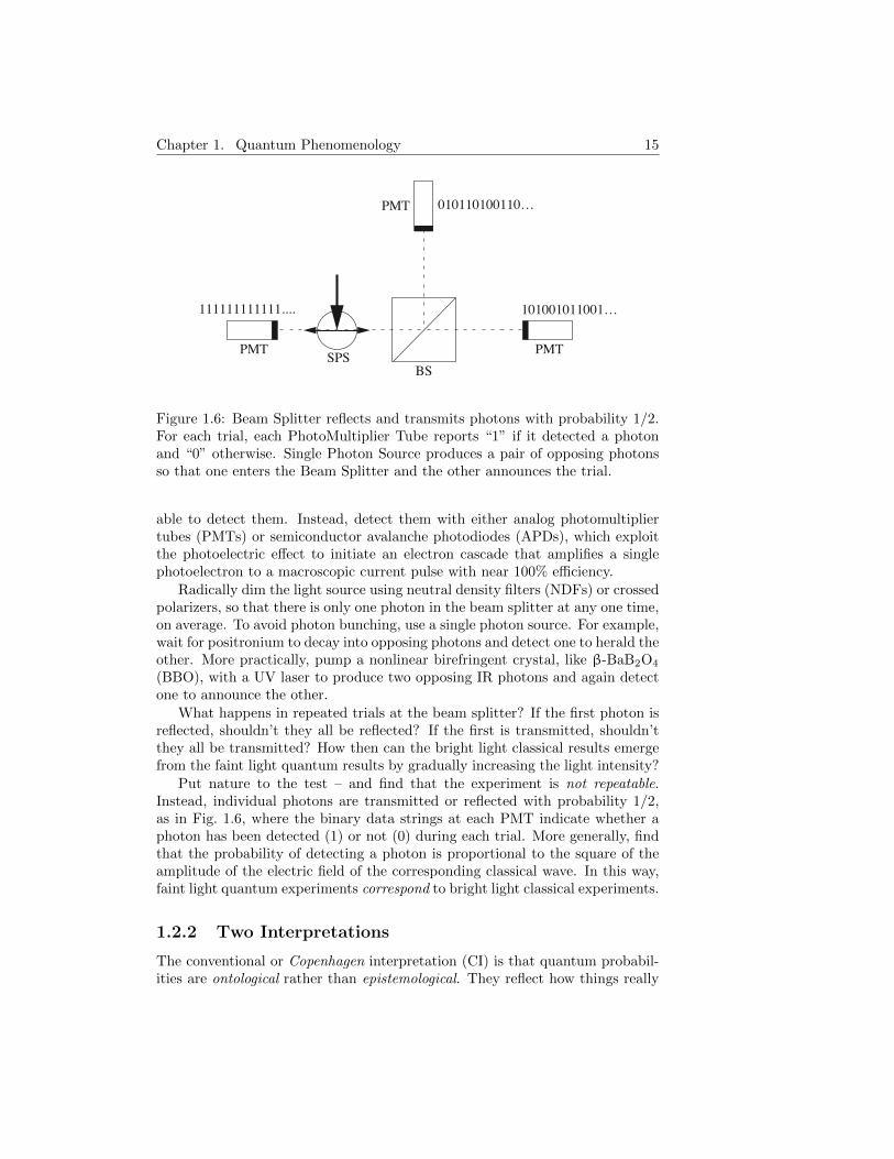
BSPMTPMT SPS
PMT 010110100110
111111111111.... 101001011001
Figure 1.6: Beam Splitter reflects and transmits photons with probability 1/2.For each trial, each PhotoMultiplier Tube reports “1” if it detected a photonand “0” otherwise. Single Photon Source produces a pair of opposing photonsso that one enters the Beam Splitter and the other announces the trial.
able to detect them. Instead, detect them with either analog photomultipliertubes (PMTs) or semiconductor avalanche photodiodes (APDs), which exploitthe photoelectric effect to initiate an electron cascade that amplifies a singlephotoelectron to a macroscopic current pulse with near 100% efficiency.
Radically dim the light source using neutral density filters (NDFs) or crossedpolarizers, so that there is only one photon in the beam splitter at any one time,on average. To avoid photon bunching, use a single photon source. For example,wait for positronium to decay into opposing photons and detect one to herald theother. More practically, pump a nonlinear birefringent crystal, like β-BaB2O4
(BBO), with a UV laser to produce two opposing IR photons and again detectone to announce the other.
What happens in repeated trials at the beam splitter? If the first photon isreflected, shouldn’t they all be reflected? If the first is transmitted, shouldn’tthey all be transmitted? How then can the bright light classical results emergefrom the faint light quantum results by gradually increasing the light intensity?
Put nature to the test – and find that the experiment is not repeatable.Instead, individual photons are transmitted or reflected with probability 1/2,as in Fig. 1.6, where the binary data strings at each PMT indicate whether aphoton has been detected (1) or not (0) during each trial. More generally, findthat the probability of detecting a photon is proportional to the square of theamplitude of the electric field of the corresponding classical wave. In this way,faint light quantum experiments correspond to bright light classical experiments.
1.2.2 Two Interpretations
The conventional or Copenhagen interpretation (CI) is that quantum probabil-ities are ontological rather than epistemological. They reflect how things really

Chapter 1. Quantum Phenomenology 16
are, not merely what can be known about them. They are inherent in nature,not merely limitations in the measuring apparatus.
Einstein famously objected, “God does not play dice with the universe”.In the post-Einstein Many Worlds interpretation (MWI), the ontological
probabilities are eliminated. Instead, each photon is both transmitted and re-flected, and the world splits into two histories, one for each possibility! Epis-temological randomness is apparent only to observers, like physicists, confinedto single histories. From a God’s eye perspective, the MWI is deterministicand, for the beam splitter, symmetric (both of two equally likely possibilitiesare realized), but at the ontological expense of invoking an uncountable infinityof equally real worlds to explain the single observable world.
There are other interpretations, but none preserve classical reality.
1.2.3 Mach-Zehnder Interferometer
Probabilities alone don’t exhaust the novelty of quantum reality.Recombine the light from a beam splitter using two mirrors and a second
beam splitter, as in Fig. 1.7. Such a device is called a Mach-Zehnder interfer-ometer. If “T” and “R” represent “transmitted” and “reflected”, then the fourpaths through the interferometer can be denoted RRR, TRT, RRT, TRR, wherethe first two paths exit up and the second two paths exit right. All paths havethe same length, but each transmission and reflection is accompanied by a phaseshift that depends on the details of the optics. However, light waves interfereconstructively when exiting right (and, by energy conservation, destructivelywhen exiting up), because the corresponding paths involve the same number oftransmissions and the same number of reflections. (In practice, a dielectric slabin one path of the interferometer can be rotated slightly to adjust the phaseshifts. Also, if one of the mirrors or beam splitters is slightly canted, then theinterference produces a fringe pattern of parallel stripes.)
Figure 1.7: Mirrors (left) and a second beam splitter (right) recombine brightlight split by the first beam splitter.
Radically dim the light source so that only one photon is in the interferom-eter at any one time, as in Fig. 1.8. What happens? Without the recombining

Chapter 1. Quantum Phenomenology 17
beam splitter, the data strings at the PMTs are perfectly anticorrelated butrandom. With the recombining beam splitter, the data strings are still per-fectly anticorrelated but are now homogeneous, and all photons exit right, inagreement with the high intensity experiment. Apparently, there is interferenceeven with only one photon in the apparatus at a time!
Figure 1.8: Mirrors (left) and a second beam splitter (right) recombine photonpaths split by the first beam splitter.
Note how the addition of the recombining beam splitter radically alters theoutput of the device. If individual photons were somehow “splitting” (or not)at the first beam splitter, how could they know whether (or not) the recom-bining beams splitter was in place? In fact, since the speed of the photons isc ∼ 109 km/hr ∼ 0.3 m/ns, nanosecond electronics in a table-top experimentcan decide to remove or introduce the recombining beam splitter after the pho-ton has interacted with the first beam splitter! The results of such delayedchoice experiments are exactly the same: in those trials with the recombiner,all photons exit right; in those trials without the recombiner, half the photonsexit right and half exit up.
Try to check the paths taken by the photons. Since each photon carriesmomentum p = h/λ, if one of the two mirrors floats or glides on a low-frictionsurface, then the mirror’s recoil (or not) reveals the photon’s path. However,in such which-way experiments, the constructive and destructive interference,which makes all photons exit right and none exit up, is destroyed, and insteadhalf the photons exit right and half exit up. Indeed, which-way information isconsistent with the particle nature of light but is inconsistent with the wave na-ture of light. Particles take definite paths and do not interfere, while waves takeall paths and do interfere. Apparently, incompatible experimental arrangementselicit complementary aspects of the wave-particle duality of light: which-way in-formation (no recombiner or floating mirrors) elicits the particle aspect of light,while no which-way information (recombiner and fixed mirrors) elicits the waveaspect of light.
Chapter 1. Quantum Phenomenology 18
1.2.4 Quantum Eraser
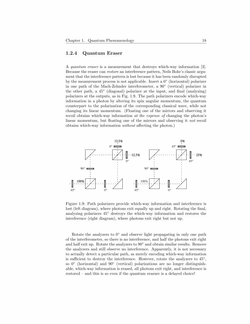
A quantum eraser is a measurement that destroys which-way information [3].Because the eraser can restore an interference pattern, Neils Bohr’s classic argu-ment that the interference pattern is lost because it has been randomly disruptedby the measurement process is not applicable. Insert a 0◦ (horizontal) polarizerin one path of the Mach-Zehnder interferometer, a 90◦ (vertical) polarizer inthe other path, a 45◦ (diagonal) polarizer at the input, and final (analyzing)polarizers at the outputs, as in Fig. 1.9. The path polarizers encode which-wayinformation in a photon by altering its spin angular momentum, the quantumcounterpart to the polarization of the corresponding classical wave, while notchanging its linear momentum. (Floating one of the mirrors and observing itrecoil obtains which-way information at the expense of changing the photon’slinear momentum, but floating one of the mirrors and observing it not recoilobtains which-way information without affecting the photon.)
0
90
0
0
45
100%
12.5%
12.5%
0
90
45
45
45
100%
0%
25%
Figure 1.9: Path polarizers provide which-way information and interference islost (left diagram), where photons exit equally up and right. Rotating the final,analyzing polarizers 45◦ destroys the which-way information and restores theinterference (right diagram), where photons exit right but not up.
Rotate the analyzers to 0◦ and observe light propagating in only one pathof the interferometer, so there is no interference, and half the photons exit rightand half exit up. Rotate the analyzers to 90◦ and obtain similar results. Removethe analyzers and still observe no interference. Apparently, it is not necessaryto actually detect a particular path, as merely encoding which-way informationis sufficient to destroy the interference. However, rotate the analyzers to 45◦,so 0◦ (horizontal) and 90◦ (vertical) polarizations are no longer distinguish-able, which-way information is erased, all photons exit right, and interference isrestored – and this is so even if the quantum erasure is a delayed choice!
Chapter 1. Quantum Phenomenology 19
1.2.5 Interaction-Free Measurement
Floating one of the two mirrors in the Mach-Zehnder interferometer loses single-photon interference, even if the single photon reflects off the other, stationarymirror. How can the floating mirror affect the photon if the photon doesn’teven come near it or exchange energy with it? Quantum physics allows us totest counterfactuals, things that might have happened but did not!
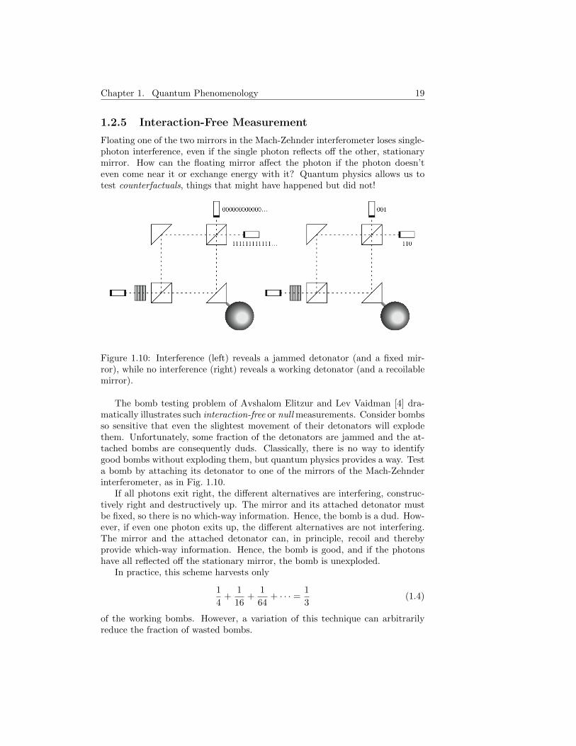
Figure 1.10: Interference (left) reveals a jammed detonator (and a fixed mir-ror), while no interference (right) reveals a working detonator (and a recoilablemirror).
The bomb testing problem of Avshalom Elitzur and Lev Vaidman [4] dra-matically illustrates such interaction-free or null measurements. Consider bombsso sensitive that even the slightest movement of their detonators will explodethem. Unfortunately, some fraction of the detonators are jammed and the at-tached bombs are consequently duds. Classically, there is no way to identifygood bombs without exploding them, but quantum physics provides a way. Testa bomb by attaching its detonator to one of the mirrors of the Mach-Zehnderinterferometer, as in Fig. 1.10.
If all photons exit right, the different alternatives are interfering, construc-tively right and destructively up. The mirror and its attached detonator mustbe fixed, so there is no which-way information. Hence, the bomb is a dud. How-ever, if even one photon exits up, the different alternatives are not interfering.The mirror and the attached detonator can, in principle, recoil and therebyprovide which-way information. Hence, the bomb is good, and if the photonshave all reflected off the stationary mirror, the bomb is unexploded.
In practice, this scheme harvests only
1
4+
1
16+
1
64+ · · · = 1
3(1.4)
of the working bombs. However, a variation of this technique can arbitrarilyreduce the fraction of wasted bombs.
Chapter 1. Quantum Phenomenology 20
1.2.6 Quantum Computing
Classically, distinguishing a real coin, with a head and a tail, from a trick coin,with two heads (or two tails) requires looking at each side separately and thencomparing the results. However, David Deutsch’s “two-bit” quantum algorithmcan do this all at once!
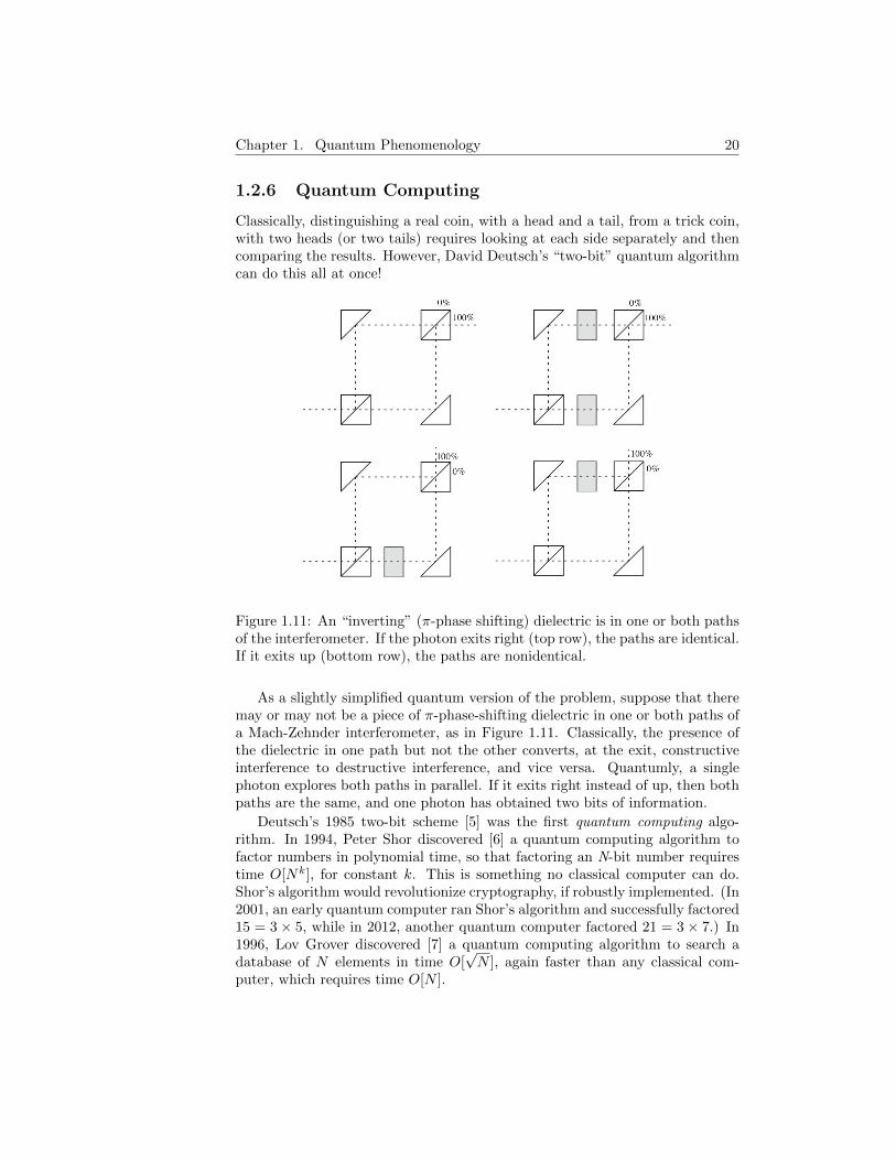
Figure 1.11: An “inverting” (π-phase shifting) dielectric is in one or both pathsof the interferometer. If the photon exits right (top row), the paths are identical.If it exits up (bottom row), the paths are nonidentical.
As a slightly simplified quantum version of the problem, suppose that theremay or may not be a piece of π-phase-shifting dielectric in one or both paths ofa Mach-Zehnder interferometer, as in Figure 1.11. Classically, the presence ofthe dielectric in one path but not the other converts, at the exit, constructiveinterference to destructive interference, and vice versa. Quantumly, a singlephoton explores both paths in parallel. If it exits right instead of up, then bothpaths are the same, and one photon has obtained two bits of information.
Deutsch’s 1985 two-bit scheme [5] was the first quantum computing algo-rithm. In 1994, Peter Shor discovered [6] a quantum computing algorithm tofactor numbers in polynomial time, so that factoring an N-bit number requirestime O[Nk], for constant k. This is something no classical computer can do.Shor’s algorithm would revolutionize cryptography, if robustly implemented. (In2001, an early quantum computer ran Shor’s algorithm and successfully factored15 = 3× 5, while in 2012, another quantum computer factored 21 = 3× 7.) In1996, Lov Grover discovered [7] a quantum computing algorithm to search adatabase of N elements in time O[
√N ], again faster than any classical com-
puter, which requires time O[N ].
Chapter 1. Quantum Phenomenology 21
The MWI provides an easy heuristic for understanding the source of theadvantage of these quantum algorithms: they distribute the calculations amongmany parallel universes!
1.2.7 Mach-Zehnder Classical Model
Prior to creating a more explicit quantum model of the Mach-Zehnder interfer-ometer, first create a more quantitative classical model. At high intensity, lightis split into two wave trains at the first beam splitter, which are recombined atthe second beam splitter and exit up and right. Let the electric field magnitudeat the entrance be
E [0, t] = E0 cos[ωt], (1.5)
where t is the time elapsed, and ω = 2π/T is the temporal frequency of thewave train. Then, the electric field magnitude at the exit due to the wave trainreflected by mirror n is
En[z, t] =1√2
1√2E0 cos[ωt− kz + δn], (1.6)
where z = 2` is the distance traveled, k = 2π/λ is the spatial frequency, and δnis the extra phase shift due to reflections. Since ω/k = λ/T = c, the spacetimephase ϕ = ωt − kz = k(ct − z) is zero at z = ct, and hence represents a wavetraveling in the z direction at speed c. The factors of 1/
√2 are due to the beam
splitters. The total electric field magnitude at the exit is the superposition
E = E1 + E2 =1√2
1√2E0(cos[ϕ+ δ1] + cos[ϕ+ δ2]). (1.7)
Eyes and cameras are sensitive to the time-averaged square of this electric field,which is the intensity
I = 〈E2〉 =1
2
1
2
⟨E20(cos2[ϕ+ δ1] + 2 cos[ϕ+ δ1] cos[ϕ+ δ2] + cos2[ϕ+ δ2]
)⟩.
(1.8)Using the trigonometric identity 2 cosu cos v = cos[u + v] + cos[u − v], thisbecomes
I =1
2E20
⟨cos2[ϕ+ δ1]
⟩+⟨cos[2ϕ+ δ1 + δ2]
⟩+⟨cos[δ1 − δ2]
⟩+⟨cos2[ϕ+ δ2]
⟩2
.
(1.9)Since the time average of a sinusoid (over an integer number of periods) vanishes,and the time average of the square of a sinusoid is 1/2,
I = I01 + cos δ
2, (1.10)
where I0 = E20 〈cos2[ωt]〉 = E20/2 is the entrance intensity and δ = δ1 − δ2 is thedifference between the reflection phase shifts of the two paths.
Chapter 1. Quantum Phenomenology 22
Assume there is a phase shift of π/2 radians at each reflection. (The actualphase shifts depend on the detailed characteristics of the optical elements, butcan always be adjusted by inserting dielectric slabs in one or both paths of theinterferometer). At the up exit, the difference in phase shifts δ = 3(π/2) −(π/2) = π, and so the intensity I = 0. At the right exit, the difference in phaseshifts δ = 2(π/2)− 2(π/2) = 0, and so the intensity I = I0.
1.2.8 Mach-Zehnder Quantum Model 1
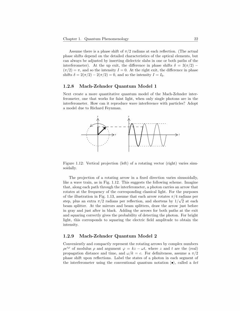
Next create a more quantitative quantum model of the Mach-Zehnder inter-ferometer, one that works for faint light, when only single photons are in theinterferometer. How can it reproduce wave interference with particles? Adopta model due to Richard Feynman.
Figure 1.12: Vertical projection (left) of a rotating vector (right) varies sinu-soidally.
The projection of a rotating arrow in a fixed direction varies sinusoidally,like a wave train, as in Fig. 1.12. This suggests the following scheme. Imaginethat, along each path through the interferometer, a photon carries an arrow thatrotates at the frequency of the corresponding classical light. For the purposesof the illustration in Fig. 1.13, assume that each arrow rotates π/4 radians perstep, plus an extra π/2 radians per reflection, and shortens by 1/
√2 at each
beam splitter. At the mirrors and beam splitters, draw the arrow just beforein gray and just after in black. Adding the arrows for both paths at the exitand squaring correctly gives the probability of detecting the photon. For brightlight, this corresponds to squaring the electric field amplitude to obtain theintensity.
1.2.9 Mach-Zehnder Quantum Model 2
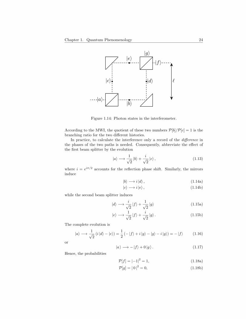
Conveniently and compactly represent the rotating arrows by complex numbersρeiϕ of modulus ρ and argument ϕ = kz − ωt, where z and t are the (real)propagation distance and time, and ω/k = c. For definiteness, assume a π/2phase shift upon reflections. Label the states of a photon in each segment ofthe interferometer using the conventional quantum notation |•〉, called a ket

Chapter 1. Quantum Phenomenology 23
Figure 1.13: A photon carries an imaginary arrow that rotates at the frequencyof the corresponding classical light. Adding the arrows at the exit for bothpaths and squaring gives the probability of detecting the photon: unity forexiting right (top row) and zero for exiting up (bottom row).
(from the word bracket), as in Fig. 1.14. At the first beam splitter, the initialphoton state |a〉 evolves to a quantum superposition of a transmitted photonstate |b〉 and a reflected photon state |c〉. If ` is the length of one segment of theinterferometer, and the photon is at the first beam splitter at z = 0 and t = 0,then
|a〉 −→ 1√2ei(k`/2−ωt) |b〉+
1√2ei(k`/2−ωt+π/2) |c〉 . (1.11)
The complex numbers multiplying each state record the amplitude and phaseof the rotating arrows: the moduli 1/
√2 account for the passage through the
beam splitter, while the π/2 in the argument of the second complex numberaccounts for the reflection phase shift.
According to the CI, if the experiment were stopped here, and the photon’stransmittance or reflectance observed, the square of the moduli of these complexnumbers would be the corresponding probabilities
P[b] =
∣∣∣∣ 1√2ei(k`/2−ωt)
∣∣∣∣2 =1
2, (1.12a)
P[c] =
∣∣∣∣ 1√2ei(k`/2−ωt+π/2)
∣∣∣∣2 =1
2. (1.12b)
Chapter 1. Quantum Phenomenology 24
Figure 1.14: Photon states in the interferometer.
According to the MWI, the quotient of these two numbers P[b]/P[c] = 1 is thebranching ratio for the two different histories.
In practice, to calculate the interference only a record of the difference inthe phases of the two paths is needed. Consequently, abbreviate the effect ofthe first beam splitter by the evolution
|a〉 −→ 1√2|b〉+
i√2|c〉 , (1.13)
where i = eiπ/2 accounts for the reflection phase shift. Similarly, the mirrorsinduce
|b〉 −→ i |d〉 , (1.14a)
|c〉 −→ i |e〉 , (1.14b)
while the second beam splitter induces
|d〉 −→ i√2|f〉+
1√2|g〉 (1.15a)
|e〉 −→ 1√2|f〉+
i√2|g〉 . (1.15b)
The complete evolution is
|a〉 −→ 1√2
(i |d〉 − |e〉) =1
2(− |f〉+ i |g〉 − |g〉 − i |g〉) = − |f〉 (1.16)
or|a 〉 −→ − |f〉+ 0 |g 〉 . (1.17)
Hence, the probabilities
P[f ] = |−1|2 = 1, (1.18a)
P[g] = | 0 |2 = 0, (1.18b)

Chapter 1. Quantum Phenomenology 25
as expected. The certainty of |f〉 (exiting right) and the impossibility of |g〉(exiting up) is an example of quantum interference.
1.3 Measurement & Entanglement
Light elucidates the measurement problem and quantum entanglement.
1.3.1 Hilbert Space Preview
In general, if |ϕ〉 and |ψ〉 are quantum states, then any linear combinationa|ϕ〉+ b|ψ〉, with complex coefficients a and b, is also a quantum state. In fact,such states form a Hilbert space: a linear vector space with a complex scalarproduct. For example, the calcite crystal of Section 1.1 can induce a photon toevolve to a state |ψ〉 that is a superposition of horizontal |h〉 and vertical |v〉polarization, namely
|ψ〉 = a |h〉+ b |v〉 , (1.19)
where |a|2 + |b|2 = 1 to conserve probability. (Measurement will certainly findthe photon in one of the two states.) The set of all such states form a quantumbit or qubit, which is of fundamental importance in quantum computing: whilea classical bit can be in one of two states, a qubit can be in an infinite numberof superpositions of states.
A quantum superposition is a kind of complex-number-weighted coexistenceof possibilities (or potentialities). According to the CI, the absolute squareof the weights correspond to the probabilities of measuring the alternatives.According to the MWI, the quotient of the weights is the branching ratio forthe two different histories. (The branching ratio must be a rational number,but rationals can approximate real numbers arbitrarily well.)
1.3.2 Quantum Evolution
As shown below, superpositions evolve continuously and deterministically underthe Schrodinger differential equation, in both the CI and the MWI. For example,
|ψ〉 S−→ |ψ′〉 = a′ |h〉+ b′ |v〉 . (1.20)
In the CI, but not in the MWI, there is also a discontinuous and probabilisticcollapse of a superposition to classical probability-weighted alternatives whenthe system is measured (or observed or registered). For example,
|ψ′ 〉 M−→
|h 〉 , P[h] = |a′|2
|v 〉 , P[v] = |b′|2
. (1.21)
While the S-evolution is uncontroversial, the same cannot be said about theM-evolution.
Chapter 1. Quantum Phenomenology 26
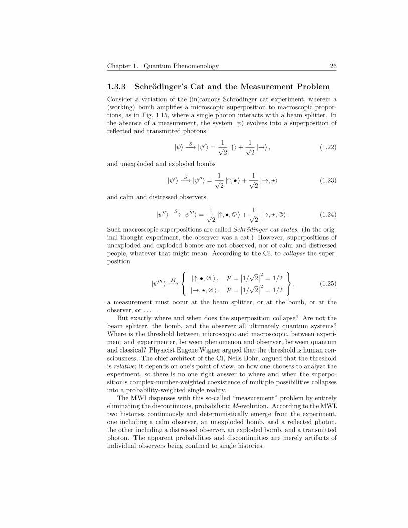
1.3.3 Schrodinger’s Cat and the Measurement Problem
Consider a variation of the (in)famous Schrodinger cat experiment, wherein a(working) bomb amplifies a microscopic superposition to macroscopic propor-tions, as in Fig. 1.15, where a single photon interacts with a beam splitter. Inthe absence of a measurement, the system |ψ〉 evolves into a superposition ofreflected and transmitted photons
|ψ〉 S−→ |ψ′〉 =1√2|↑〉+
1√2|→〉 , (1.22)
and unexploded and exploded bombs
|ψ′〉 S−→ |ψ′′〉 =1√2|↑, •〉+
1√2|→, ?〉 (1.23)
and calm and distressed observers
|ψ′′〉 S−→ |ψ′′′〉 =1√2|↑, •,, 〉+
1√2|→, ?,/〉 . (1.24)
Such macroscopic superpositions are called Schrodinger cat states. (In the orig-inal thought experiment, the observer was a cat.) However, superpositions ofunexploded and exploded bombs are not observed, nor of calm and distressedpeople, whatever that might mean. According to the CI, to collapse the super-position
|ψ′′′ 〉 M−→
|↑, •,, 〉 , P =∣∣1/√2
∣∣2 = 1/2
|→, ?,/ 〉 , P =∣∣1/√2
∣∣2 = 1/2
, (1.25)
a measurement must occur at the beam splitter, or at the bomb, or at theobserver, or . . . .
But exactly where and when does the superposition collapse? Are not thebeam splitter, the bomb, and the observer all ultimately quantum systems?Where is the threshold between microscopic and macroscopic, between experi-ment and experimenter, between phenomenon and observer, between quantumand classical? Physicist Eugene Wigner argued that the threshold is human con-sciousness. The chief architect of the CI, Neils Bohr, argued that the thresholdis relative; it depends on one’s point of view, on how one chooses to analyze theexperiment, so there is no one right answer to where and when the superpo-sition’s complex-number-weighted coexistence of multiple possibilities collapsesinto a probability-weighted single reality.
The MWI dispenses with this so-called “measurement” problem by entirelyeliminating the discontinuous, probabilistic M-evolution. According to the MWI,two histories continuously and deterministically emerge from the experiment,one including a calm observer, an unexploded bomb, and a reflected photon,the other including a distressed observer, an exploded bomb, and a transmittedphoton. The apparent probabilities and discontinuities are merely artifacts ofindividual observers being confined to single histories.
Chapter 1. Quantum Phenomenology 27
Figure 1.15: Single photon incident on a beam splitter is reflected and detectedby a PMT, calming the observer (left), or is transmitted and detonates a bomb,distressing the observer (right). The S-evolution places the photon, the bomb,and the observer in a macroscopic quantum superposition, a Schrodinger catstate.
1.3.4 Polarization
Beam splitters and mirrors control the direction of classical light and the lin-ear momenta of photons. Calcite crystals, quarter wave plates, and polarizerscontrol the polarization of classical light and the angular momenta (or spin) ofphotons. This latter capability facilitates investigation of additional aspects ofquantum reality.
In classical optics, polarization refers to the oscillation of the light’s electricfield. If light is traveling in the z-direction at speed c = ω/k, then
~Eh[δh] = x E0 cos[kz − ωt+ δh], (1.26a)
~Ev[δv] = y E0 cos[kz − ωt+ δv] , (1.26b)
represent horizontal and vertical linearly polarized light, because the electricfield is oscillating in a line. Superpose this light with different relative phasesδh − δv to create differently polarized light. For example, if the relative phaseshift is zero, then
~Ed = ~Eb[0] + ~Ev[0] = (x+ y) E0 cos[kz − ωt] , (1.27)
represents diagonally polarized light, which is just linearly polarized light in adifferent direction. If the relative phase shift is ±π/2, then
~Er = ~Eh[0] + ~Ev[+π/2] = (x cos[kz − ωt]− y sin[kz − ωt]) E0, (1.28a)
~E` = ~Eh[0] + ~Ev[−π/2] = (x cos[kz − ωt] + y sin[kz − ωt]) E0, (1.28b)
represent right hand and left hand circularly polarized light, because the electricfield rotates in a circle at each place in space. In the particle physics convention,

Chapter 1. Quantum Phenomenology 28
at each place, right hand light rotates as the right hand fingers curl when theright thumb points in the propagation direction. The corresponding relationsfor photons correspond to the classical relations for light waves. A “diagonal”photon is a superposition
|d〉 =1√2|h〉+
1√2|v〉 . (1.29)
“Circular” or natural photons are the superpositions
|r〉 =1√2|h〉+
i√2|v〉 , (1.30a)
|`〉 =1√2|h〉 − i√
2|v〉 , (1.30b)
where the ±i = e±iπ/2 account for the relative phase shifts. Since photons arenaturally circular, it is appropriate to invert these relations and write
|h〉 =1√2
(|r〉+ |`〉) , (1.31a)
|v〉 =−i√
2(|r〉 − |`〉) . (1.31b)
In a measurement of the linear polarization of |v〉, |r〉 and |`〉 are equally likely,
|v 〉 M−→
|r 〉 , P =∣∣−i/√2
∣∣2 = 1/2
|` 〉 , P =∣∣+i/√2
∣∣2 = 1/2
, (1.32)
but the complex numbers ±i are crucial to recovering |r〉 when superposing |h〉and |v〉, as in Eq. 1.30a.
Measuring the linear polarization of a photon places it in a superposition ofright and left circular polarizations, while measuring the circular polarizationplaces the photon in a superposition of linear polarizations. In fact, a photoncannot have both linear and circular polarization simultaneously; knowing onetype of polarization leaves the other type indeterminate, a special case of theHeisenberg indeterminacy principle.
Optically anisotropic materials with different indices of refraction in differentdirections can transform light from one polarization to another. A calcite crystalcan convert a diagonal light beam into parallel beams of horizontal and verticallight. A quarter wave plate can convert diagonal light into circular light (byretarding one component by a distance λ/4).
1.3.5 Crossed Polarizers
An ideal polarizer converts unpolarized light into linearly polarized light byselectively transmitting only one polarization. Consider light traveling in thez-direction, and linearly polarized in the x-direction, incident on a polarizer with

Chapter 1. Quantum Phenomenology 29
transmission axis an angle θ from the x-direction, as in Figure 1.16. If the trans-mission direction is x′ and the perpendicular direction is y′, then decompose theincident electric field amplitude as the superposition
~E0 = x′E0 cos θ + y′E0 sin θ. (1.33)
Therefore, the transmitted amplitude is
E ′0 = E0 cos θ (1.34)
and, since intensity is proportional to the amplitude squared, the transmittedintensity is
I ′ = Icos2θ, (1.35)
which is Malus’s Law.
Figure 1.16: A polarizer transmits the component of light parallel to its trans-mission axis.
Similarly, a photon polarized in the x-direction is a superposition of a photonpolarized in the parallel and perpendicular directions,
|x〉 = cos θ |x′〉+ sin θ |y′〉 . (1.36)
Therefore
|x 〉 M−→
|x′ 〉 , P = |cos θ|2 = cos2θ
|y′ 〉 , P = |sin θ|2 = sin2θ
, (1.37)
and hence the probability of transmission is cos2θ, which corresponds to Malus’slaw.
Consider next a single photon incident on crossed polarizers, as in Fig. 1.17.If the probability of transmission at the first polarizer is 1/2 and the proba-bility of transmission at the second polarizer is cos2θ, then the probability oftransmission through both polarizers is (1/2)cos2θ. If the relative angle betweenthe two transmission axes is θ = π/2, then no photons get through. However,
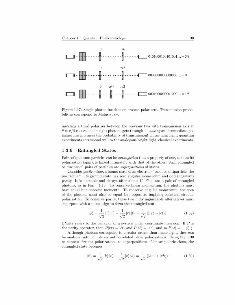
Chapter 1. Quantum Phenomenology 30
Figure 1.17: Single photon incident on crossed polarizers. Transmission proba-bilities correspond to Malus’s law.
inserting a third polarizer between the previous two with transmission axis atθ = π/4 causes one in eight photons gets through — adding an intermediate po-larizer has increased the probability of transmission! These faint light, quantumexperiments correspond well to the analogous bright light, classical experiments.
1.3.6 Entangled States
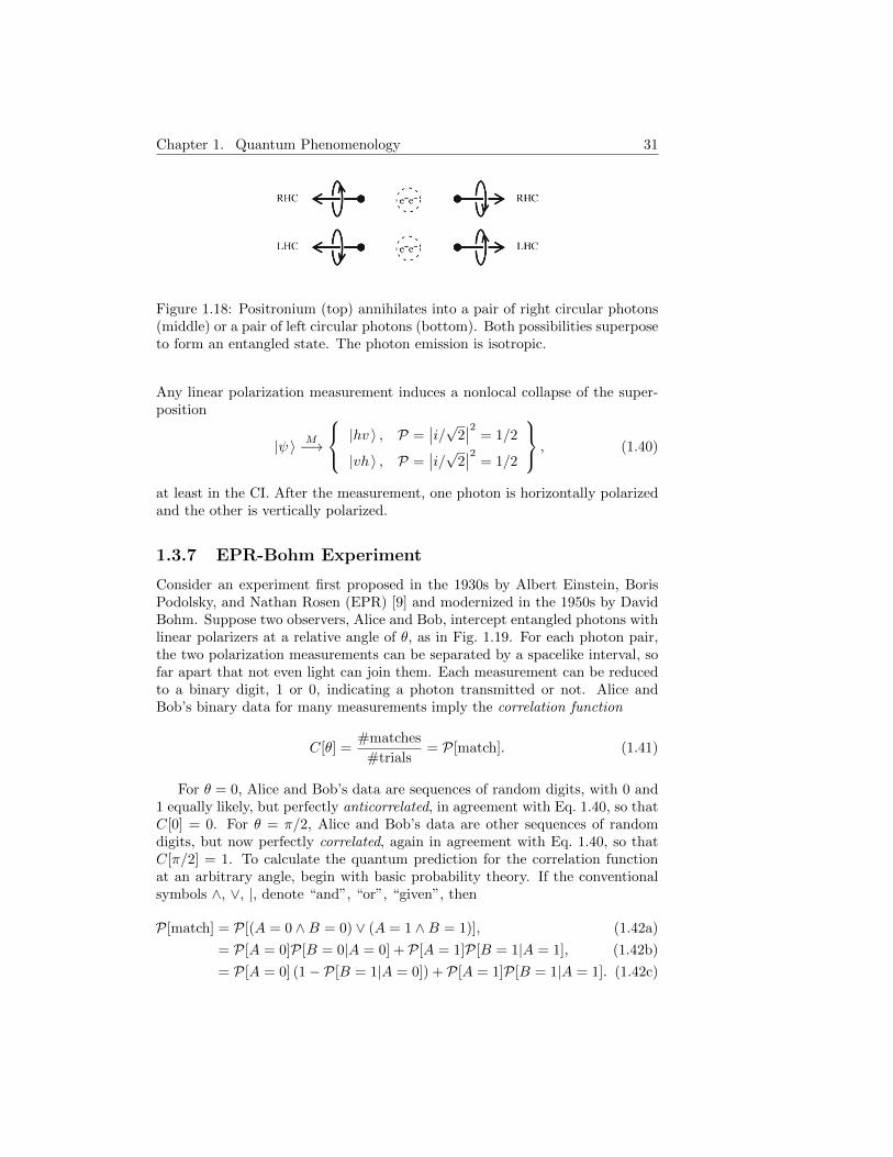
Pairs of quantum particles can be entangled so that a property of one, such as itspolarization (spin), is linked intimately with that of the other. Such entangledor “twinned” pairs of particles are superpositions of states.
Consider positronium, a bound state of an electron e- and its antiparticle, thepositron e+. Its ground state has zero angular momentum and odd (negative)parity. It is unstable and decays after about 10−10 s into a pair of entangledphotons, as in Fig. 1.18. To conserve linear momentum, the photons musthave equal but opposite momenta. To conserve angular momentum, the spinof the photons must also be equal but opposite, implying identical circularpolarization. To conserve parity, these two indistinguishable alternatives mustsuperpose with a minus sign to form the entangled state
|ψ〉 =1√2|r〉 |r〉 − 1√
2|`〉 |`〉 =
1√2
(|rr〉 − |``〉) . (1.38)
(Parity refers to the behavior of a system under coordinate inversion. If P isthe parity operator, then P |rr〉 = |``〉 and P |``〉 = |rr〉, and so P |ψ〉 = −|ψ〉.)
Although photons correspond to circular rather than linear light, they canbe analyzed into completely anticorrelated plane polarizations. Using Eq. 1.30to express circular polarizations as superpositions of linear polarizations, theentangled state becomes
|ψ〉 =i√2|h〉 |v〉+
i√2|v〉 |h〉 =
i√2
(|hv〉+ |vh〉) . (1.39)
Chapter 1. Quantum Phenomenology 31
Figure 1.18: Positronium (top) annihilates into a pair of right circular photons(middle) or a pair of left circular photons (bottom). Both possibilities superposeto form an entangled state. The photon emission is isotropic.
Any linear polarization measurement induces a nonlocal collapse of the super-position
|ψ 〉 M−→
|hv 〉 , P =∣∣i/√2
∣∣2 = 1/2
|vh 〉 , P =∣∣i/√2
∣∣2 = 1/2
, (1.40)
at least in the CI. After the measurement, one photon is horizontally polarizedand the other is vertically polarized.
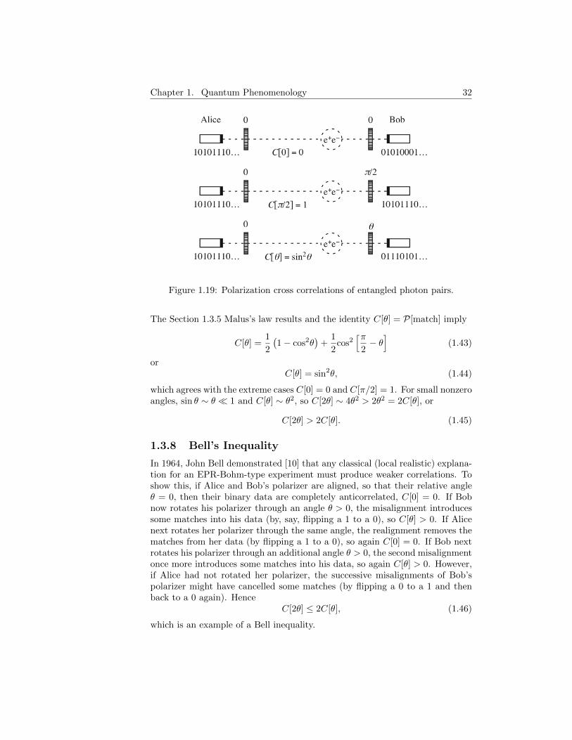
1.3.7 EPR-Bohm Experiment
Consider an experiment first proposed in the 1930s by Albert Einstein, BorisPodolsky, and Nathan Rosen (EPR) [9] and modernized in the 1950s by DavidBohm. Suppose two observers, Alice and Bob, intercept entangled photons withlinear polarizers at a relative angle of θ, as in Fig. 1.19. For each photon pair,the two polarization measurements can be separated by a spacelike interval, sofar apart that not even light can join them. Each measurement can be reducedto a binary digit, 1 or 0, indicating a photon transmitted or not. Alice andBob’s binary data for many measurements imply the correlation function
C[θ] =#matches
#trials= P[match]. (1.41)
For θ = 0, Alice and Bob’s data are sequences of random digits, with 0 and1 equally likely, but perfectly anticorrelated, in agreement with Eq. 1.40, so thatC[0] = 0. For θ = π/2, Alice and Bob’s data are other sequences of randomdigits, but now perfectly correlated, again in agreement with Eq. 1.40, so thatC[π/2] = 1. To calculate the quantum prediction for the correlation functionat an arbitrary angle, begin with basic probability theory. If the conventionalsymbols ∧, ∨, |, denote “and”, “or”, “given”, then
P[match] = P[(A = 0 ∧B = 0) ∨ (A = 1 ∧B = 1)], (1.42a)
= P[A = 0]P[B = 0|A = 0] + P[A = 1]P[B = 1|A = 1], (1.42b)
= P[A = 0] (1− P[B = 1|A = 0]) + P[A = 1]P[B = 1|A = 1]. (1.42c)
Chapter 1. Quantum Phenomenology 32
Figure 1.19: Polarization cross correlations of entangled photon pairs.
The Section 1.3.5 Malus’s law results and the identity C[θ] = P[match] imply
C[θ] =1
2
(1− cos2θ
)+
1
2cos2
[π2− θ]
(1.43)
orC[θ] = sin2θ, (1.44)
which agrees with the extreme cases C[0] = 0 and C[π/2] = 1. For small nonzeroangles, sin θ ∼ θ � 1 and C[θ] ∼ θ2, so C[2θ] ∼ 4θ2 > 2θ2 = 2C[θ], or
C[2θ] > 2C[θ]. (1.45)
1.3.8 Bell’s Inequality
In 1964, John Bell demonstrated [10] that any classical (local realistic) explana-tion for an EPR-Bohm-type experiment must produce weaker correlations. Toshow this, if Alice and Bob’s polarizer are aligned, so that their relative angleθ = 0, then their binary data are completely anticorrelated, C[0] = 0. If Bobnow rotates his polarizer through an angle θ > 0, the misalignment introducessome matches into his data (by, say, flipping a 1 to a 0), so C[θ] > 0. If Alicenext rotates her polarizer through the same angle, the realignment removes thematches from her data (by flipping a 1 to a 0), so again C[0] = 0. If Bob nextrotates his polarizer through an additional angle θ > 0, the second misalignmentonce more introduces some matches into his data, so again C[θ] > 0. However,if Alice had not rotated her polarizer, the successive misalignments of Bob’spolarizer might have cancelled some matches (by flipping a 0 to a 1 and thenback to a 0 again). Hence
C[2θ] ≤ 2C[θ], (1.46)
which is an example of a Bell inequality.
Chapter 1. Quantum Phenomenology 33
The quantum prediction of Eq. 1.45 contradicts the classical prediction ofEq. 1.46, so put nature to the test. By the 1980s, in a culmination of a seriesof increasingly better experiments by many research groups, Alain Aspect andcolleagues convincingly demonstrated that Bell’s inequality is decisively violatedin these kind of experiments. Consequently, there must be something wrongwith Bell’s argument, as Bell himself anticipated.
The argument seems to rest on two assumptions: locality and reality. Local-ity means no superluminal connections, so what happens here and now doesn’tdepend on what happens then and there. For example, the argument implic-itly assumes locality when it reasons that, when Bob rotates his polarizer, healters his data but not Alice’s, and vice versa. Reality means counterfactualdefiniteness, the ability to consistently discuss what might have happened butdid not. For example, the argument reasons that if Bob had rotated his polar-izer through θ, then he would have introduced some matches, and if he had thenrotated through an additional θ, then some of the matches might have cancelled.One of these two classically reasonable assumptions must be wrong.
A popular nonlocal interpretation of the EPR-Bohm experiment is that it isimpossible to force a two-particle interpretation on an entangled particle pair.While this may violate the spirit of special relativity, it does not violate theletter of special relativity. In the CI, quantum randomness prevents using en-tangled states for superluminal telegraphs, because any message introduced byrotating one of the polarizers is found only in the correlations between possiblyremote and spacelike experiments. In the MWI, measurements don’t collapsesuperpositions, nonlocally or otherwise, and locality is restored.

Chapter 1. Quantum Phenomenology 34
Problems
1. Complex numbers are used extensively in quantum physics. Commonnotations are
z = x+ iy = r(cos θ + i sin θ) = reiθ, (1.47)
and a fundamental operation is complex conjugation
z∗ = z = x− iy = r(cos θ − i sin θ) = re−iθ, (1.48)
where i =√−1. Find the principal values of the following numbers in the
form x+ iy, where x, y ∈ R are real numbers.
(a)1
1 + i.
(b) 25e2i (Caution: The angle is 2 radians not 2π radians.)
(c)3i− 7
i+ 4(Caution: The numerator is not 3− 7i.)
(d)
(1 + i
1− i
)2718
(Hint: Don’t use a calculator or computer!)
(e)√i
(f) ii
2. Prove the following equations.
(a) eiθ = cos θ + i sin θ (Hint: Use Taylor series expansions.)
(b) eiπ + 1 = 0 (Euler’s tombstone.)
(c) sin θ =eiθ − e−iθ
2i
(d) cos θ =eiθ + e−iθ
2
3. Malus’s law and the inverse quantum Zeno effect. Consider asequence of N + 1 polarizers each rotated at an angle π/2N relative to itsneighbors. Suppose a photon passes through the first polarizer.
(a) What is the probability that it passes through the second polarizer?(Hint: Consult Eq. 1.37.)
(b) What is the probability that it passes through all the rest of thepolarizers?
(c) Show that the probability of transmission increases to unity as thenumber of polarizers increases to infinity. Thus, a dense set of “mea-surements” can rotate the photon’s plane of polarization through aright angle!

Chapter 1. Quantum Phenomenology 35
4. Experimental interaction-free measurements. A nonlinear opticalcrystal down-converts a UV laser photon to a pair of low-energy photonstraveling 30◦ from each other. The detection of one confirms the existenceof the other, which is directed into a Michelson interferometer (left below).Without the “Medusa” mirror in the interferometer’s orthogonal path,virtually all photons exit the way they came, with virtually no photonsexiting down, due to destructive interference.
(a) With the Medusa mirror in place, what fraction of photons exit down,thereby registering the Medusa without seeing it?
(b) By reducing the beam splitter’s reflection probability p� 1/2, whatfraction of measurements can be made interaction-free? (Hint: Ex-clude cases where a photon exits the way it enters.)
5. Improved null measurements. This interferometer (right above) ex-ploits the inverse quantum Zeno effect. Time the switchable mirror toallow the photon to go back-and-forth through the system N times. Sugarwater rotates the polarization plane π/4N each time the photon passesthrough it. The time-reversible polarizing beam splitter sends horizontallyand vertically polarized light in orthogonal directions. Input photons arehorizontally polarized.
(a) By how much does the sugar water rotate the polarization when thephoton pass back and forth through it?
(b) When the vertical path is clear of the “Medusa” bomb, why does thephoton exit the system vertically polarized?
(c) When the Medusa blocks the vertical path, why does the photon exitnearly horizontally polarized (when it isn’t absorbed) for large N?
(d) Now quantitatively, with what probability does the Medusa not ab-sorb the photon when it blocks the vertical path?
(e) Consequently, what fraction of measurements are interaction-free asN →∞?
Chapter 1. Quantum Phenomenology 36
6. Photon Polarization. First consider classic light propagating in thez-direction.
(a) Show that
~ER = E0(x cos[kz − ωt] + y cos[kz − ωt+ π/2]), (1.49a)
~EL = E0(x cos[kz − ωt] + y cos[kz − ωt− π/2]), (1.49b)
represent right and left circularly polarized light. Hint: Sketch therotation of the electric fields at a fixed point in space.
(b) Show that
~Ex = ~EL + ~ER, (1.50a)
~Ey = ~EL − ~ER, (1.50b)
represent linear polarized light.
(c) Express circular light as linear superpositions of linear light.
(d) In order to correspond with classical light, assume that circularlypolarized photons are superpositions of linearly polarized photonsand their states are related by
|r〉 =1√2|x〉+
1√2e+iπ/2|y〉, (1.51a)
|`〉 =1√2|x〉+
1√2e−iπ/2|y〉. (1.51b)
Show that
|x〉 =1√2|`〉+
1√2|r〉, (1.52a)
|y〉 =i√2|`〉 − i√
2|r〉. (1.52b)
(e) Rotate the coordinate system through an angle ϕ in the xy-plane.Justify
|x′〉 = + cosϕ|x〉+ sinϕ|y〉, (1.53a)
|y′〉 = − sinϕ|x〉+ cosϕ|y〉. (1.53b)
(f) Show that the rotated circular polarizations satisfy
|r′〉 = e−iϕ|r〉, (1.54a)
|`′〉 = e+iϕ|`〉. (1.54b)
(g) Show then that the probability of measuring a circularly polarizedphoton to have a particular linear polarization is the same at anyangle. Why is this so physically?

Chapter 1. Quantum Phenomenology 37
7. Create a single photon model of the Fig. 1.9 quantum eraser. Assumean initial diagonal polarization state |D〉 = (|h〉 + |v〉)/
√2. The effect
of the vertical polarizer is |ψ〉 → |v〉〈v|ψ〉, where the complex “bra-ket”scalar products 〈v|v〉 = 1 and 〈h|v〉∗ = 〈v|h〉 = 0, for example. Gen-eralizing Section 1.2.9, track both location and polarization by work-ing in the product Hilbert space |LP 〉 = |L〉|P 〉 ∈ HL ⊗ HP , where〈Lh|L′v〉 = 〈L|L′〉〈h|v〉 = 0, for example. Track phase shifts by modelingthe beam splitter with transmission and reflection coefficients t = 1/
√2
and r = i/√
2.
(a) Compute the probabilities for the photon to exit up and right withthe analyzers horizontal.
(b) Compute the probabilities for the photon to exit up and right withthe analyzers diagonal.

Chapter 1. Quantum Phenomenology 38
Chapter 2
Hilbert Spaces
Generalize Euclidean space to mathematically describe quantum phenomena.
2.1 Euclidean Space
The familiar real scalar product defines distances and angles. Completeness(the inclusion of all limited points) makes possible calculus. If places
~u,~v, ~w ∈ R3 (2.1)
and real coefficientsa, b, c ∈ R, (2.2)
then the linear superposition
a~u+ b~v + c~w ∈ R3. (2.3)
is also a place. Use the real and symmetric scalar or dot product
~u · ~v = ~v · ~u ∈ R (2.4)
to define an orthonormal basis
xm · xn = m · n = δmn. (2.5)
Decompose a vector
~v = v1x1 + v2x2 + v3x3 =∑n
vnxn =∑n
xnvn, (2.6)
where the projectionsvn = xn · ~v ∈ R (2.7)
imply
~v = x1(x1 · ~v) + x2(x2 · ~v) + x3(x3 · ~v) =∑n
xn (xn · ~v) (2.8)
andv2 = ~v · ~v =
∑n
(xn · ~v) (xn · ~v) =∑n
(xn · ~v)2
=∑n
v2n. (2.9)
39

Chapter 2. Hilbert Spaces 40
2.2 Generic Hilbert Space
2.2.1 Vectors
To describe quantum phenomena requires more general n-dimensional Hilbertspaces H equipped with complex scalar products. (If x, y ∈ R are real numbersand i =
√−1, then z = x+ iy ∈ C is a complex number, and z∗ = z = x− iy is
its complex conjugate.) In conventional Dirac bra(c)ket notation, if states
|ϕ〉, |χ〉, |ψ〉 ∈ H, (2.10)
(pronounced “ket phi, ket chi, ket psi”) and complex coefficients
a, b, c ∈ C, (2.11)
then the linear superposition
a|ϕ〉+ b|χ〉+ c|ψ〉 ∈ H (2.12)
is also a state. Use the complex symmetric scalar product
〈ϕ|ψ〉 = 〈ψ|ϕ〉∗ ∈ C (2.13)
(pronounced “bra phi ket psi equals bra psi ket phi star”) to define an orthonor-mal basis
〈ψm|ψn〉 = 〈m|n〉 = δmn, (2.14)
where the Kronecker delta
δmn =
1 : m = n
0 : m 6= n
. (2.15)
Decompose a state
|ψ〉 = ψ1|1〉+ ψ2|2〉+ · · · =∑n
ψn|n〉 =∑n
|n〉ψn, (2.16)
where the projectionsψn = 〈n|ψ〉 ∈ C (2.17)
imply
|ψ〉 = |1〉〈1|ψ〉+ |2〉〈2|ψ〉+ · · · =∑n
|n〉〈n|ψ〉. (2.18)
and
〈ψ|ψ〉 =∑n
〈ψ|n〉〈n|ψ〉 =∑n
〈n|ψ〉∗〈n|ψ〉 =∑n
|〈n|ψ〉|2 =∑n
|ψn|2. (2.19)
Among other advantages, the bra ket notation makes it easy to label stateswithout needing to miniaturize the text in a subscript; for example,
|0〉 = |ψ0〉 = |ground state〉. (2.20)
Chapter 2. Hilbert Spaces 41
2.2.2 Operators
In the Hilbert spaces H, scalar products map vectors to numbers, and operatorsmap vectors to vectors. If operators
A,B,C ∈ L[H], (2.21)
then they linearly
A (a|ϕ〉+ b|χ〉+ c|ψ〉) = aA|ϕ〉+ bA|χ〉+ cA|ψ〉 (2.22)
map vectors to other vectors
A|ψ〉 = |ψ′〉, (2.23)
or vectors to multiples of vectors
A|ψa〉 = a|ψa〉, (2.24)
which can be abbreviated as
A|a〉 = a|a〉, (2.25)
where |a〉 ∈ H is an eigenvector or eigenstate of A and a ∈ C is the correspondingeigenvalue or eigenscalar. The set of all eigenvalues {a} of A is the spectrum ofA.
2.2.3 Dual Space
In a countable Hilbert space, every ket |ψ〉 ∈ H corresponds to a bra in the dualspace, |ψ〉† = 〈ψ| ∈ H∗ (pronounced “ket psi dagger equals bra psi in h star”).Every operator A that maps kets to kets
|ψ〉 −→A|ψ′〉 = A|ψ〉 ∈ H (2.26)
corresponds to an adjoint operator A† that maps bras to bras
〈ψ| −→A†〈ψ′| = 〈ψ|A† ∈ H∗. (2.27)
The adjoint reverses the order of operations. For example, if
|χ〉 ≡ B|ϕ〉, (2.28)
then
|ψ〉 ≡ AB|ϕ〉 = A|χ〉 (2.29)
so
〈ψ| = 〈ϕ|(AB)† = 〈χ|A† = 〈ϕ|B†A† (2.30)
and
(AB)† = B†A†. (2.31)
Chapter 2. Hilbert Spaces 42
The adjoint generalized complex conjugation. For example, the adjoint of acomplex number
c† = 〈ψ|ϕ〉† = |ϕ〉†〈ψ|† = 〈ϕ|ψ〉 = 〈ψ|ϕ〉∗ = c∗, (2.32)
using the Eq. 2.13 complex symmetry. Furthermore
〈ψ|A|ϕ〉∗ = 〈ψ|A|ϕ〉† = |ϕ〉†A†〈ψ|† = 〈ϕ|A†|ψ〉. (2.33)
For base states |m〉, the matrix elements
(A†)mn = 〈m|A†|n〉 = 〈n|A|m〉∗ = A∗nm. (2.34)
To adjoint an expression, reverse the order of the factors (although numberscommute with everything), interchange kets and bras, replace operators by theiradjoints and numbers by their complex conjugates.
2.2.4 Hermitian Operators
In a countable Hilbert space, Hermitian operators are self-adjoint, so
H† = H. (2.35)
Hermitian operators have real eigenvalues and orthogonal eigenstates.If
H|h〉 = h|h〉, (2.36)
then〈h|H = h∗〈h| (2.37)
implies via projection〈h|H|h〉 = h〈h|h〉 (2.38)
and〈h|H|h〉 = h∗〈h|h〉. (2.39)
The difference0 = (h− h∗)〈h|h〉 (2.40)
implies the eigenvalueh = h∗ (2.41)
is real.If there are two distinct eigenvalues, h1 6= h2 ∈ C,
H|1〉 = h1|1〉, (2.42a)
H|2〉 = h2|2〉, (2.42b)
then projection implies〈2|H|1〉 = h1〈2|1〉 (2.43)
Chapter 2. Hilbert Spaces 43
and
〈1|H|2〉 = h2〈1|2〉, (2.44a)
〈1|H|2〉∗ = (h2〈1|2〉)∗, (2.44b)
〈2|H†|1〉 = h∗2〈2|1〉, (2.44c)
〈2|H|1〉 = h2〈2|1〉. (2.44d)
The difference0 = (h1 − h2)〈2|1〉 (2.45)
implies the eigenstates〈2|1〉 = 0 (2.46)
are orthogonal.
2.2.5 Unitary Operators
The adjoint of a unitary operator is its inverse,
U† = U−1, (2.47)
soU†U = I = UU†, (2.48)
where I is the identity operator. Unitary operators have unit eigenvalues andpreserve scalar products.
IfU |u〉 = u|u〉, (2.49)
then〈u|U† = 〈u|u∗ = u∗〈u|. (2.50)
The product〈u|u〉 = 〈u|I|u〉 = 〈u|U†U |u〉 = u∗u〈u|u〉. (2.51)
implies1 = |u|2, (2.52)
so the eigenvalue is a phase factor, u = eiϕ, where ϕ ∈ R. In fact, if H is aHermitian operator, then
U = eiH ≡ I + iH − 1
2H2 − i 1
3!H3 + · · · (2.53)
is a unitary operator, where the infinite series expansion defines the exponentialof an operator. The adjoint
U† = e−iH†
= e−iH = I − iH − 1
2H2 + i
1
3!H3 + · · · , (2.54)
and because −iH and iH commute,
U†U = e−iHeiH = e−iH+iH = e0 = I, (2.55)
Chapter 2. Hilbert Spaces 44
and similarly UU† = I. (However, in general, if AB 6= BA, then eAeB 6= eA+B .)
If a unitary operator transforms two states
|ψ′〉 = U |ψ〉, (2.56a)
|ϕ′〉 = U |ϕ〉, (2.56b)
then their scalar product
〈ψ′|ϕ′〉 = 〈ψ|U†U |ϕ〉 = 〈ψ|ϕ〉 (2.57)
is preserved.
2.3 Matrix Representations
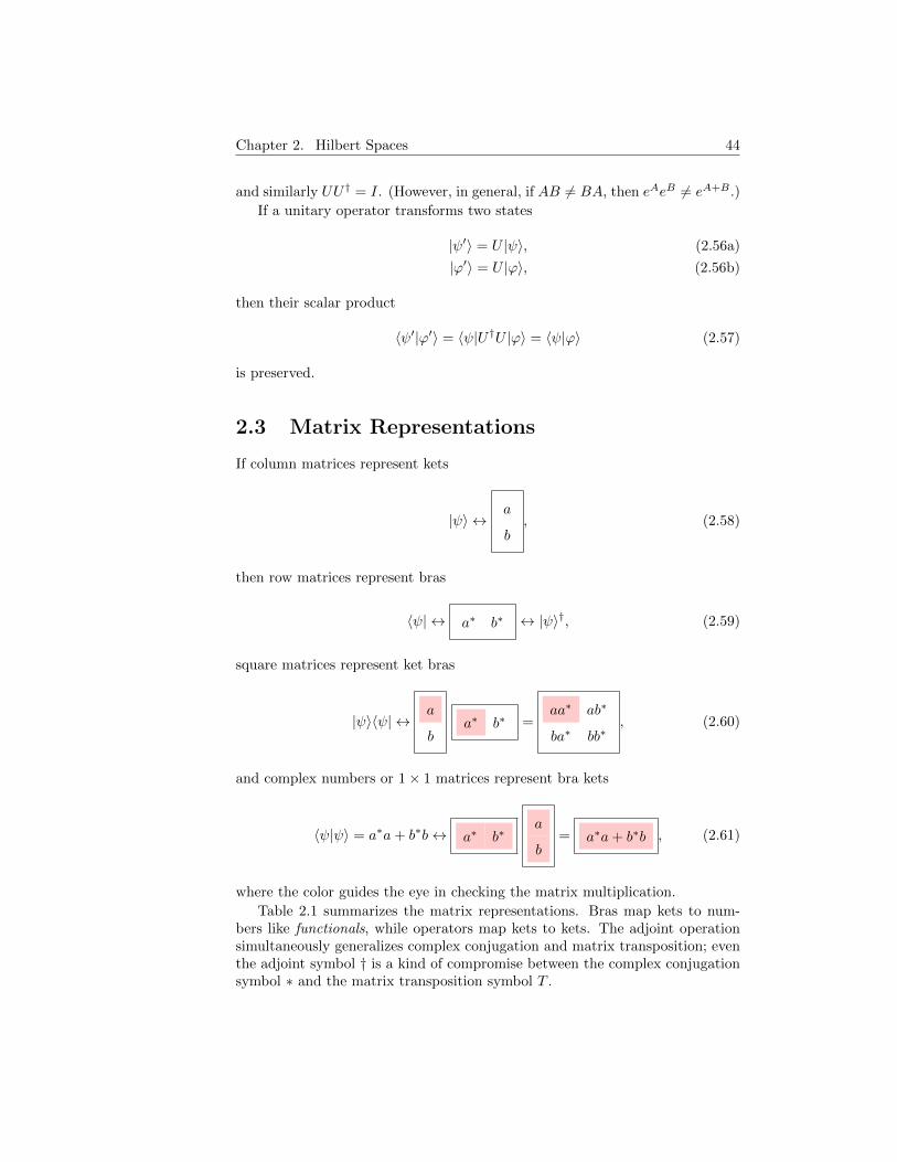
If column matrices represent kets
|ψ〉 ↔a
b, (2.58)
then row matrices represent bras
〈ψ| ↔ a∗ b∗ ↔ |ψ〉†, (2.59)
square matrices represent ket bras
|ψ〉〈ψ| ↔a
ba∗ b∗ =
aa∗ ab∗
ba∗ bb∗, (2.60)
and complex numbers or 1× 1 matrices represent bra kets
〈ψ|ψ〉 = a∗a+ b∗b↔ a∗ b∗a
b= a∗a+ b∗b , (2.61)
where the color guides the eye in checking the matrix multiplication.
Table 2.1 summarizes the matrix representations. Bras map kets to num-bers like functionals, while operators map kets to kets. The adjoint operationsimultaneously generalizes complex conjugation and matrix transposition; eventhe adjoint symbol † is a kind of compromise between the complex conjugationsymbol ∗ and the matrix transposition symbol T .
Chapter 2. Hilbert Spaces 45
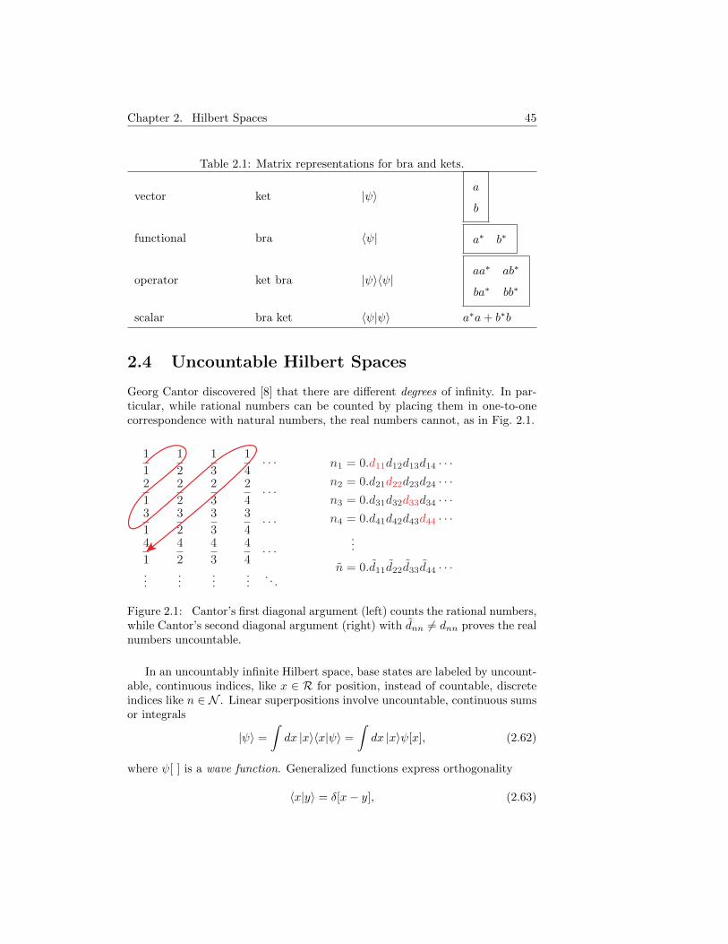
Table 2.1: Matrix representations for bra and kets.
vector ket |ψ〉a
b
functional bra 〈ψ| a∗ b∗
operator ket bra |ψ〉〈ψ|aa∗ ab∗
ba∗ bb∗
scalar bra ket 〈ψ|ψ〉 a∗a+ b∗b
2.4 Uncountable Hilbert Spaces
Georg Cantor discovered [8] that there are different degrees of infinity. In par-ticular, while rational numbers can be counted by placing them in one-to-onecorrespondence with natural numbers, the real numbers cannot, as in Fig. 2.1.
Figure 2.1: Cantor’s first diagonal argument (left) counts the rational numbers,while Cantor’s second diagonal argument (right) with dnn 6= dnn proves the realnumbers uncountable.
In an uncountably infinite Hilbert space, base states are labeled by uncount-able, continuous indices, like x ∈ R for position, instead of countable, discreteindices like n ∈ N . Linear superpositions involve uncountable, continuous sumsor integrals
|ψ〉 =
∫dx |x〉〈x|ψ〉 =
∫dx |x〉ψ[x], (2.62)
where ψ[ ] is a wave function. Generalized functions express orthogonality
〈x|y〉 = δ[x− y], (2.63)

Chapter 2. Hilbert Spaces 46
where the Dirac deltaδ[x] = lim
ε→0δε[x], (2.64)
is the limit of infinitely tall, infinitesimally thin functions that bound a unitarea,
δε[x] =
1/ε : |x| < ε/2
0 : |x| > ε/2
. (2.65)
The Dirac delta’s resulting normalization
1 =
∫ ∞−∞
dx δ[x− x0] (2.66)
implies the sifting property∫ ∞−∞
dx δ[x− x0]ψ[x] = ψ[x0]
∫ ∞−∞
dx δ[x− x0] = ψ[x0]. (2.67)
For example, project Eq. 2.62 onto the state |y〉 to get
〈y|ψ〉 =
∫dx 〈y|x〉ψ[x] =
∫dx δ[x− y]ψ[x] = ψ[y]. (2.68)
Table 2.2 compares countable and uncountable bases.
Table 2.2: Comparison between discrete and continuous bases formulas.
property discrete or countable continuous or uncountable
orthogonality 〈m|n〉 = δmn 〈x|y〉 = δ[x− y]
sifting ψn =∑m ψmδmn ψ[y] =
∫∞−∞ dx δ[x− y]ψ[x]
closure |ψ〉 =∑m |m〉〈m|ψ〉 |ψ〉 =
∫dx |x〉〈x|ψ〉
2.5 Quantum Example
As an example of the quantum Hilbert space formalism, with suggestively chosennotation, consider the energy observable H such that
H|ε〉 = ε|ε〉. (2.69)
Since the operator H = H† is hermitian, its eigenvalues ε = ε∗ ∈ H are real.Assume an initial state as a symmetric superposition of orthonormal eigenstates
|ψ0〉 =1√2|ε1〉+
1√2|ε2〉 ≡ |s〉 (2.70)
Chapter 2. Hilbert Spaces 47
normalized such that
〈ψ0|ψ0〉 =
(1√2〈ε1|+
1√2〈ε2|)(
1√2|ε1〉+
1√2|ε2〉)
=1
2〈ε1|ε1〉+
1
2〈ε1|ε2〉+
1
2〈ε2|ε1〉+
1
2〈ε2|ε2〉
=1
2+ 0 + 0 +
1
2= 1. (2.71)
Given a norm-preserving unitary time translation operator
Ut = e−itH/~, (2.72)
with real parameter t ∈ R and dimensional constant ~, the state at a later time
|ψt〉 = Ut|ψ0〉 = e−itH/~|ψ0〉 =1√2e−itH/~|ε1〉+
1√2e−itH/~|ε2〉
=1√2e−itε1/~|ε1〉+
1√2e−itε2/~|ε2〉. (2.73)
The amplitude for again observing the initial symmetric state is the projection
〈s|ψt〉 =
(1√2〈ε1|+
1√2〈ε2|)(
1√2e−itε1/~|ε1〉+
1√2e−itε2/~|ε2〉
)=
1
2e−itε1/~ +
1
2e−itε2/~, (2.74)
and the probability is the absolute square
Ps = |〈s|ψt〉|2
=
(1
2e+itε1/~ +
1
2e+itε2/~
)(1
2e−itε1/~ +
1
2e−itε2/~
)=
1
4+
1
4e+it(ε1−ε2)/~ +
1
4e−it(ε1−ε2)/~ +
1
4
=1
2+
1
2cos
[tε1 − ε2
~
]= cos2
[ε1 − ε2
2~t
]. (2.75)
In quantum mechanics, normalized vectors represent states and complexvector projections represent probability amplitudes. The absolute square ofamplitudes represent probabilities. Hermitian operators represent observablesand their real eigenvalues represent observed values. Unitary operators representtransformations like translations and rotations.

Chapter 2. Hilbert Spaces 48
2.6 Commutation
Let A = A† and B = B† be Hermitian operators representing observable quan-tities like energy and momentum. If they commute, so that AB = BA and theircommutator
[A,B] = AB −BA = 0 (2.76)
vanishes, then they share common eigenstates and can be known exactly si-multaneously. If they do not commute, the measurement of one “contaminates”measurement of the other, and perfectly knowing one leaves the other completelyindeterminate.
Assume the operators do commute, and let |a〉 be an eigenstate of A witheigenvalue a,
A|a〉 = a|a〉. (2.77)
The vanishing of the commutator implies the vanishing of the matrix elements
0 = 〈a|[A,B]|a′〉 = 〈a|AB|a′〉 − 〈a|BA|a′〉 = (a− a′)〈a|B|a′〉. (2.78)
If the eigenvalues a 6= a′ are nondegenerate (or can be made so), then 〈a|B|a′〉 =0 and the operator B is “diagonal” in the {|a〉} basis,
〈a|B|a′〉 = Baa′δaa′ ≡ b〈a|a′〉. (2.79)
Since this is true for all |a〉,B|a′〉 = b|a′〉, (2.80)
and |a′〉 = |a′, b〉 is also an eigenstate of B,
A|a, b〉 = a|a, b〉, (2.81a)
B|a, b〉 = b|a, b〉. (2.81b)
Now assume the operators do not commute. If the state |ψ〉 =∑|a〉ψa ∈
H characterizes the system, then the probability of measuring the observablecorresponding to the operator A and getting the result a is
Pa = |〈a|ψ〉|2 = |ψa|2, (2.82)
the average or mean of many such measurements on identical systems is
〈A〉 = 〈ψ|A|ψ〉 =∑a,a′
〈a′|A|a〉ψ∗a′ψa =∑a,a′
aδa′,aψ∗a′ψa =
∑a
a|ψa|2 =∑a
aPa,
(2.83)and the spread or uncertainty in the results is the standard deviation
∆A =√⟨
(A− 〈A〉I)2⟩
=√⟨
(A− 〈A〉)2⟩. (2.84)
Remove the mean from the operators by defining
A0 = A− 〈A〉, (2.85a)
B0 = B − 〈B〉. (2.85b)

Chapter 2. Hilbert Spaces 49
Define the linear combination
C0 = A0 − iεB0, (2.86)
where ε ∈ R is a real number, and the state
|ϕ〉 = C0|ψ〉 (2.87)
so that
0 ≤ 〈ϕ|ϕ〉 = 〈ψ|C†0C0|ψ〉= 〈ψ|(A0 + iεB0)(A0 − iεB0)|ψ〉= 〈ψ|A2
0 − iεA0B0 + iεB0A0 + ε2B20 |ψ〉
= 〈A20〉 − ε〈i[A0, B0]〉+ ε2〈B2
0〉= ∆A2 − ε〈i[A,B]〉+ ε2∆B2. (2.88)
This quadratic equation in ε defines a vertical parabola confined to the upper-half plane. Since it cannot cross the ε axis, it cannot have two real roots, andits quadratic discriminant must be non-positive,
D = 〈i[A,B]〉2 − 4∆A2∆B2 ≤ 0. (2.89)
Hence, the product of the uncertainties
∆A∆B ≥ 1
2
∣∣∣∣⟨i[A,B]⟩∣∣∣∣, (2.90)
which is conventionally known as the (generalized) Heisenberg uncertainty prin-ciple. For example, if two operators Q and P have the commutator
[Q,P ] = i~I, (2.91)
then the products of the uncertainties in measurements of the correspondingobservables satisfy
∆Q∆P ≥ 1
2~, (2.92)
so if one is certain, say ∆Q = 0, the other is indeterminate, ∆P =∞.
Chapter 2. Hilbert Spaces 50
Problems
1. Given the states
|ψ〉 = 3i|1〉+ 2|2〉, (2.93a)
|ϕ〉 = 2|1〉+ i|2〉, (2.93b)
and the Section 2.3 standard matrix representation
〈1| ↔ 1 0 , (2.94a)
〈2| ↔ 0 1 , (2.94b)
evaluate the following both with and without the representation.
(a) 〈ψ|ϕ〉(b) 〈ϕ|ψ〉(c) |ψ〉〈ϕ|(d) |ϕ〉〈ψ|
2. Given the operator and states
A = i|1〉〈1|+ |1〉〈2|+ 2|2〉〈1|+ 3|2〉〈2|, (2.95a)
|ψ〉 = |1〉+ i|2〉 (2.95b)
|ϕ〉 = 2|1〉+ |2〉, (2.95c)
verify that 〈ψ|A†|ϕ〉 = 〈ϕ|A|ψ〉∗ both with and without a matrix repre-sentation.
3. Simplify the following by removing the dagger †. Assume c ∈ C is acomplex number and all the operators are hermitian, as in Section 2.2.4.
(a) c†
(b) (A|ψ〉)†
(c) 〈ψ|A|ϕ〉†
(d) (c〈φ|A|ψ〉|χ〉〈ψ|)†
(e) (|ψ〉 =∑n |n〉ψn)
†
(f)(|ϕ〉 =
∫dx |x〉ϕ[x]
)†(g)
(A†B†C†
)†4. Simplify the following by removing the deltas.
(a)∑∞n=1 n
2δmn
(b)∫∞−∞ dxx2δ[x− y]
(c)∫∞−∞ dx eikxδ[x]

Chapter 2. Hilbert Spaces 51
(d)∑Nn=1 δmn (Hint: 2 cases.)
(e)∫ z−∞ dx δ[x− y] (Hint: 2 cases.)
5. Let Pn = |n〉〈n| be a projection operator onto a 2-dimensional Hilbertspace.
(a) Prove that P 2n = Pn, and interpret this result graphically.
(b) Prove that Pn is hermitian.
(c) What are the (real!) eigenvalues of Pn?
(d) Find a matrix representation for Pn.
(e) Find a matrix representation for∑n Pn =
∑n |n〉〈n|. Surprised?
6. Let σy = −i|1〉〈2|+ i|2〉〈1| be a Pauli operator.
(a) Prove that σy is hermitian.
(b) Find its eigenstates and eigenvalues.
(c) Verify that its eigenvalues are real and its eigenstates are orthogonal.
(d) Find projection operators Pn onto the normalized eigenstates.
(e) Verify that these projectors satisfy the closure relation P1 + P2 = I.
7. Let σx = |1〉〈2|+ |2〉〈1| be another Pauli operator.
(a) Prove that H = ασx is hermitian, where α ∈ R is a real parameter.
(b) Prove that U = I cosα+ iσx sinα is unitary.
(c) Verify that U = eiH or equivalently I cosα+ iσx sinα = eiασx .
8. Repeat the Section 2.5 quantum example with the antisymmetric initialstate
|a〉 =1√2|ε1〉 −
1√2|ε2〉. (2.96)
9. Show that if two operators share common eigenstates, as in Eq. 2.81, theycommute.

Chapter 2. Hilbert Spaces 52
Chapter 3
Symmetry Commutators
Fundamental physical variables like energy and momentum are intimately re-lated to spacetime symmetry transformations [11, 12].
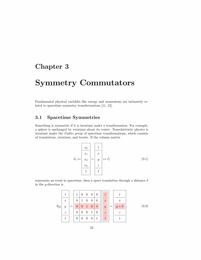
3.1 Spacetime Symmetries
Something is symmetric if it is invariant under a transformation. For example,a sphere is unchanged by rotations about its center. Nonrelativistic physics isinvariant under the Galilei group of spacetime transformations, which consistsof translations, rotations, and boosts. If the column matrix
~xt ↔
x0
x1
x2
x3
1
=
t
x
y
z
1
↔ ~rt (3.1)
represents an event in spacetime, then a space translation through a distance δin the y-direction is
Syδ
t
x
y
z
1
=
1 0 0 0 0
0 1 0 0 0
0 0 1 0 δ
0 0 0 1 0
0 0 0 0 1
t
x
y
z
1
=
t
x
y + δ
z
1
, (3.2)
53
Chapter 3. Symmetry Commutators 54
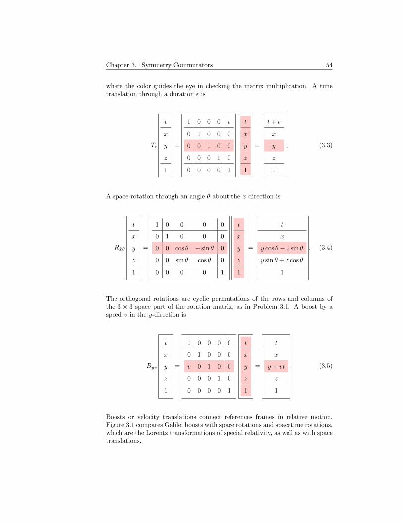
where the color guides the eye in checking the matrix multiplication. A timetranslation through a duration ε is
Tε
t
x
y
z
1
=
1 0 0 0 ε
0 1 0 0 0
0 0 1 0 0
0 0 0 1 0
0 0 0 0 1
t
x
y
z
1
=
t+ ε
x
y
z
1
, (3.3)
A space rotation through an angle θ about the x-direction is
Rxθ
t
x
y
z
1
=
1 0 0 0 0
0 1 0 0 0
0 0 cos θ − sin θ 0
0 0 sin θ cos θ 0
0 0 0 0 1
t
x
y
z
1
=
t
x
y cos θ − z sin θ
y sin θ + z cos θ
1
. (3.4)
The orthogonal rotations are cyclic permutations of the rows and columns ofthe 3 × 3 space part of the rotation matrix, as in Problem 3.1. A boost by aspeed v in the y-direction is
Byv
t
x
y
z
1
=
1 0 0 0 0
0 1 0 0 0
v 0 1 0 0
0 0 0 1 0
0 0 0 0 1
t
x
y
z
1
=
t
x
y + vt
z
1
. (3.5)
Boosts or velocity translations connect references frames in relative motion.Figure 3.1 compares Galilei boosts with space rotations and spacetime rotations,which are the Lorentz transformations of special relativity, as well as with spacetranslations.
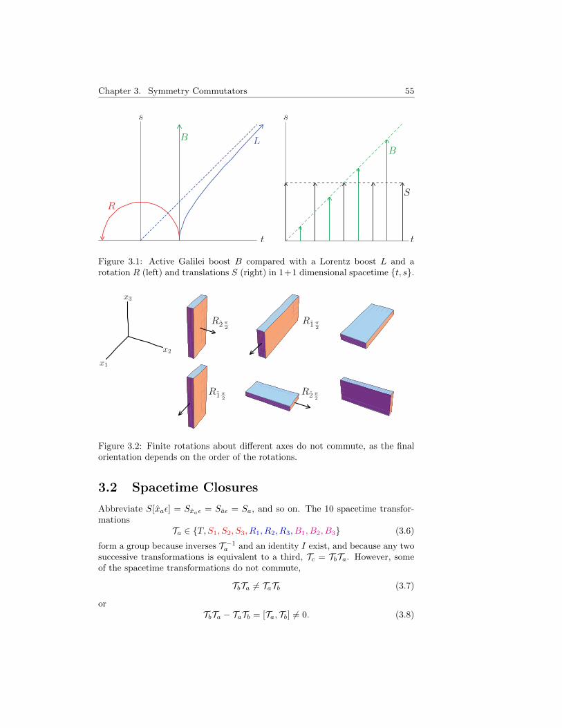
Chapter 3. Symmetry Commutators 55
Figure 3.1: Active Galilei boost B compared with a Lorentz boost L and arotation R (left) and translations S (right) in 1+1 dimensional spacetime {t, s}.
Figure 3.2: Finite rotations about different axes do not commute, as the finalorientation depends on the order of the rotations.
3.2 Spacetime Closures
Abbreviate S[xaε] = Sxaε = Saε = Sa, and so on. The 10 spacetime transfor-mations
Ta ∈ {T, S1, S2, S3, R1, R2, R3, B1, B2, B3} (3.6)
form a group because inverses T −1a and an identity I exist, and because any twosuccessive transformations is equivalent to a third, Tc = TbTa. However, someof the spacetime transformations do not commute,
TbTa 6= TaTb (3.7)
orTbTa − TaTb = [Ta, Tb] 6= 0. (3.8)
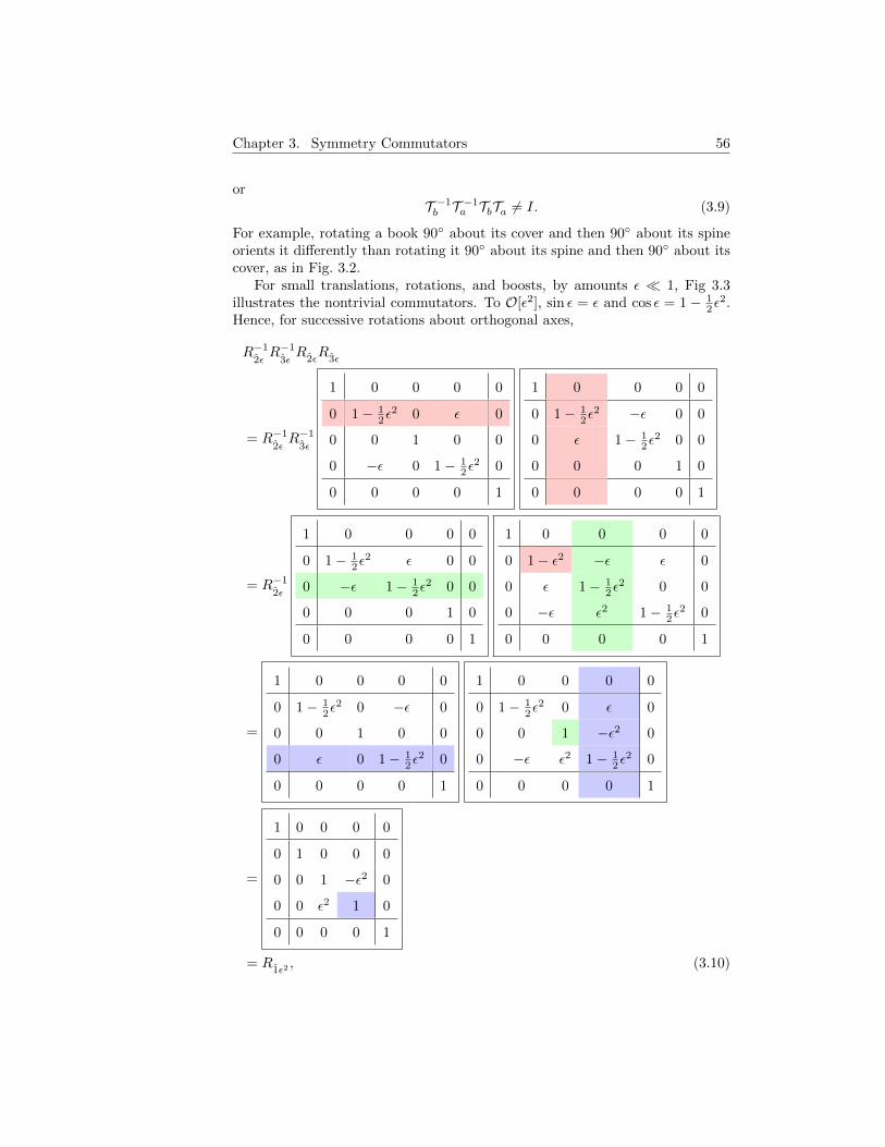
Chapter 3. Symmetry Commutators 56
orT −1b T
−1a TbTa 6= I. (3.9)
For example, rotating a book 90◦ about its cover and then 90◦ about its spineorients it differently than rotating it 90◦ about its spine and then 90◦ about itscover, as in Fig. 3.2.
For small translations, rotations, and boosts, by amounts ε � 1, Fig 3.3illustrates the nontrivial commutators. To O[ε2], sin ε = ε and cos ε = 1− 1
2ε2.
Hence, for successive rotations about orthogonal axes,
R−12εR−1
3εR
2εR
3ε
= R−12εR−1
3ε
1 0 0 0 0
0 1− 12ε
2 0 ε 0
0 0 1 0 0
0 −ε 0 1− 12ε
2 0
0 0 0 0 1
1 0 0 0 0
0 1− 12ε
2 −ε 0 0
0 ε 1− 12ε
2 0 0
0 0 0 1 0
0 0 0 0 1
= R−12ε
1 0 0 0 0
0 1− 12ε
2 ε 0 0
0 −ε 1− 12ε
2 0 0
0 0 0 1 0
0 0 0 0 1
1 0 0 0 0
0 1− ε2 −ε ε 0
0 ε 1− 12ε
2 0 0
0 −ε ε2 1− 12ε
2 0
0 0 0 0 1
=
1 0 0 0 0
0 1− 12ε
2 0 −ε 0
0 0 1 0 0
0 ε 0 1− 12ε
2 0
0 0 0 0 1
1 0 0 0 0
0 1− 12ε
2 0 ε 0
0 0 1 −ε2 0
0 −ε ε2 1− 12ε
2 0
0 0 0 0 1
=
1 0 0 0 0
0 1 0 0 0
0 0 1 −ε2 0
0 0 ε2 1 0
0 0 0 0 1
= R1ε2, (3.10)
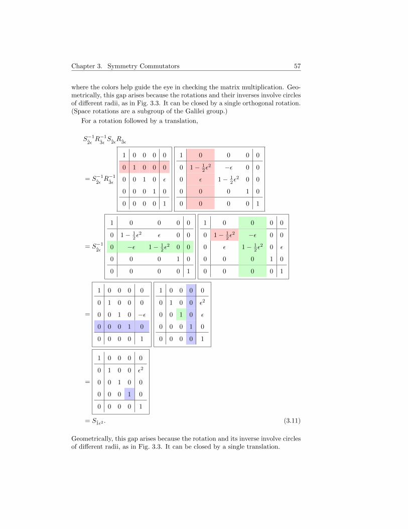
Chapter 3. Symmetry Commutators 57
where the colors help guide the eye in checking the matrix multiplication. Geo-metrically, this gap arises because the rotations and their inverses involve circlesof different radii, as in Fig. 3.3. It can be closed by a single orthogonal rotation.(Space rotations are a subgroup of the Galilei group.)
For a rotation followed by a translation,
S−12εR−1
3εS2εR
3ε
= S−12εR−1
3ε
1 0 0 0 0
0 1 0 0 0
0 0 1 0 ε
0 0 0 1 0
0 0 0 0 1
1 0 0 0 0
0 1− 12ε
2 −ε 0 0
0 ε 1− 12ε
2 0 0
0 0 0 1 0
0 0 0 0 1
= S−12ε
1 0 0 0 0
0 1− 12ε
2 ε 0 0
0 −ε 1− 12ε
2 0 0
0 0 0 1 0
0 0 0 0 1
1 0 0 0 0
0 1− 12ε
2 −ε 0 0
0 ε 1− 12ε
2 0 ε
0 0 0 1 0
0 0 0 0 1
=
1 0 0 0 0
0 1 0 0 0
0 0 1 0 −ε
0 0 0 1 0
0 0 0 0 1
1 0 0 0 0
0 1 0 0 ε2
0 0 1 0 ε
0 0 0 1 0
0 0 0 0 1
=
1 0 0 0 0
0 1 0 0 ε2
0 0 1 0 0
0 0 0 1 0
0 0 0 0 1
= S1ε2 . (3.11)
Geometrically, this gap arises because the rotation and its inverse involve circlesof different radii, as in Fig. 3.3. It can be closed by a single translation.
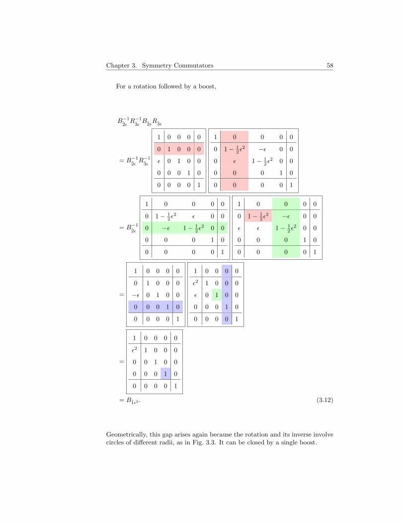
Chapter 3. Symmetry Commutators 58
For a rotation followed by a boost,
B−12εR−1
3εB
2εR
3ε
= B−12εR−1
3ε
1 0 0 0 0
0 1 0 0 0
ε 0 1 0 0
0 0 0 1 0
0 0 0 0 1
1 0 0 0 0
0 1− 12ε
2 −ε 0 0
0 ε 1− 12ε
2 0 0
0 0 0 1 0
0 0 0 0 1
= B−12ε
1 0 0 0 0
0 1− 12ε
2 ε 0 0
0 −ε 1− 12ε
2 0 0
0 0 0 1 0
0 0 0 0 1
1 0 0 0 0
0 1− 12ε
2 −ε 0 0
ε ε 1− 12ε
2 0 0
0 0 0 1 0
0 0 0 0 1
=
1 0 0 0 0
0 1 0 0 0
−ε 0 1 0 0
0 0 0 1 0
0 0 0 0 1
1 0 0 0 0
ε2 1 0 0 0
ε 0 1 0 0
0 0 0 1 0
0 0 0 0 1
=
1 0 0 0 0
ε2 1 0 0 0
0 0 1 0 0
0 0 0 1 0
0 0 0 0 1
= B1ε2 . (3.12)
Geometrically, this gap arises again because the rotation and its inverse involvecircles of different radii, as in Fig. 3.3. It can be closed by a single boost.
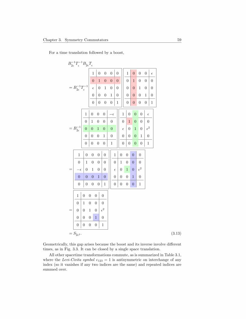
Chapter 3. Symmetry Commutators 59
For a time translation followed by a boost,
B−12εT−1εB
2εTε
= B−12εT−1ε
1 0 0 0 0
0 1 0 0 0
ε 0 1 0 0
0 0 0 1 0
0 0 0 0 1
1 0 0 0 ε
0 1 0 0 0
0 0 1 0 0
0 0 0 1 0
0 0 0 0 1
= B−12ε
1 0 0 0 −ε
0 1 0 0 0
0 0 1 0 0
0 0 0 1 0
0 0 0 0 1
1 0 0 0 ε
0 1 0 0 0
ε 0 1 0 ε2
0 0 0 1 0
0 0 0 0 1
=
1 0 0 0 0
0 1 0 0 0
−ε 0 1 0 0
0 0 0 1 0
0 0 0 0 1
1 0 0 0 0
0 1 0 0 0
ε 0 1 0 ε2
0 0 0 1 0
0 0 0 0 1
=
1 0 0 0 0
0 1 0 0 0
0 0 1 0 ε2
0 0 0 1 0
0 0 0 0 1
= S2ε2 . (3.13)
Geometrically, this gap arises because the boost and its inverse involve differenttimes, as in Fig. 3.3. It can be closed by a single space translation.
All other spacetime transformations commute, as is summarized in Table 3.1,where the Levi-Civita symbol ε123 = 1 is antisymmetric on interchange of anyindex (so it vanishes if any two indices are the same) and repeated indices aresummed over.
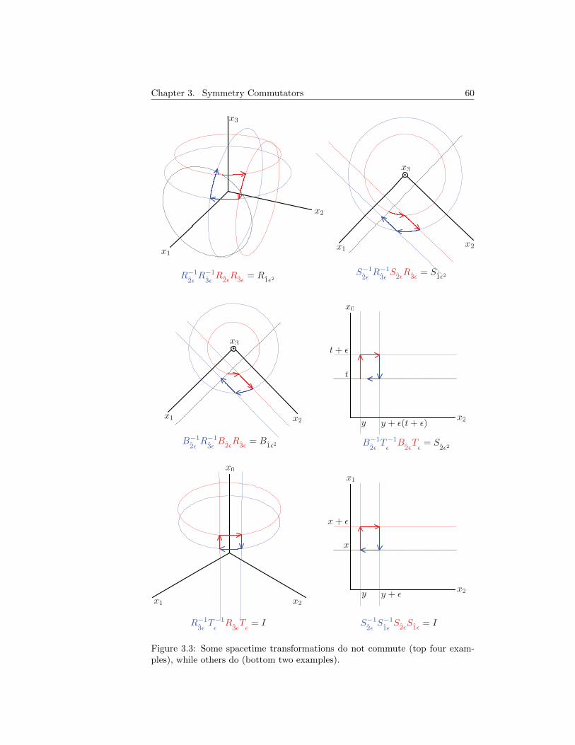
Chapter 3. Symmetry Commutators 60
Figure 3.3: Some spacetime transformations do not commute (top four exam-ples), while others do (bottom two examples).

Chapter 3. Symmetry Commutators 61
Table 3.1: Summary of nontrivial spacetime closures to O[ε2].
S−1a S−1b SaSb = I R−1a T−1RaT = I R−1a R−1b RaRb = εabcRc
B−1a B−1b BaBb = I S−1a T−1SaT = I R−1a S−1b RaSb = εabcSc
B−1a S−1b BaSb = I B−1a T−1BaT = Sa R−1a B−1b RaBb = εabcBc
3.3 State Space Symmetry Generators
3.3.1 Generic Commutator
Every spacetime transformation
T ~rt = ~r ′t , (3.14)
corresponds a state space unitary transformation
U [T ] |ψ〉 = |ψ′〉 . (3.15)
A hermitian operator H = H† generates each unitary transformation U−1 = U†
of size ε by
U[Tε]
= eiεH = I + iεH − 1
2ε2H2 + · · · , (3.16)
where
dU
dε
∣∣∣∣ε=0
= iH ≡ iT ′ε . (3.17)
Successive spacetime transformations and their inverses
T −1bεT −1aεTbεTaε
= Tcε2
(3.18)
correspond on state space to
U[T −1bε
]U[T −1aε
]U[Tbε
]U[Taε
]= U
[Tcε2
], (3.19)
In terms of the generators,
e−iεHbe−iεHaeiεHbeiεHa = eiε2Hc , (3.20)
Chapter 3. Symmetry Commutators 62
which to O[ε2] is
I + iε2Hc
=
(I − iεHb −
1
2ε2H2
b
)(I − iεHa −
1
2ε2H2
a
)×(
I + iεHb −1
2ε2H2
b
)(I + iεHa −
1
2ε2H2
a
)=
(I − iε(Hb +Ha)− ε2HbHa −
1
2ε2(H2
b +H2a)
)×(
I + iε(Hb +Ha)− ε2HbHa −1
2ε2(H2
b +H2a)
)= I − 2ε2HbHa + ε2(�
�H2b +HbHa +HaHb +@@H
2a )− ε2(�
�H2b +@@H
2a )
= I + ε2(−HbHa +HaHb)
= I + ε2[Ha, Hb], (3.21)
so the commutator of the hermitian generators
[Ha, Hb] = iHc. (3.22)
However, a shift of Ha → Ha + ϕI in the generators implies an unobservableshift |ϕ〉 → eiϕ|ψ〉 in the states along with the more general commutator
[Ha, Hb] = iHc + iϕI. (3.23)
3.3.2 Commutator Antisymmetries
Commutators, and commutators involving commutators, are antisymmetric.Add
[A,B] =��AB −HHBA, (3.24a)
[B,A] =HHBA −��AB, (3.24b)
to get[A,B] + [B,A] = 0 (3.25)
or[A,B] = −[B,A]. (3.26)
Add
[[A,B], C] = [AB −BA,C] =���ABC −���BAC −���CAB +XXXCBA, (3.27a)
[[C,A], B] = [CA−AC,B] =���CAB −XXXACB −XXXBCA +���BAC , (3.27b)
[[B,C], A] = [BC − CB,A] =XXXBCA −XXXCBA −���ABC +XXXACB, (3.27c)
Chapter 3. Symmetry Commutators 63
to get the Jacobi identity
[[A,B], C] + [[B,C], A] + [[C,A], B] = 0 (3.28)
or[[A,B], C] = [[C,B], A] + [[A,C], B]. (3.29)
Furthermore, commutators of hermitian operators are antihermitian. As-sume A† = A and B† = B. If [A,B] = C, then
C† = (AB−BA)† = (AB)†−(BA)† = B†A†−A†B† = BA−AB = −C. (3.30)
Thus, if [A,B] = iH, then H is hermitian.
3.3.3 Phase Constants
Table 3.2 summarizes the tentative generator commutation relations with thereal phase constants ϕnab ∈ R (where n is an index and not an exponent). Thecommutator relations allow the phase constants to be zeroed in all but one case.
Table 3.2: Nontrivial symmetry generator commutators with phase constants.
[S′a, S′b] = iϕ1
abI [R′a, T′] = iϕ4
a0I [R′a, R′b] = iεabcR
′c + iϕ7
abI
[B′a, B′b] = iϕ2
abI [S′a, T′] = iϕ5
a0I [R′a, S′b] = iεabcS
′c + iϕ8
abI
[B′a, S′b] = iϕ3
abI [B′a, T′] = iS′a + iϕ6
a0I [R′a, B′b] = iεabcB
′c + iϕ9
abI
Eliminable
Commutator antisymmetry implies that every operator commutes with itself,[A,A] = −[A,A] implies [A,A] = 0. Hence ϕnaa = 0.
In fact, all the phase constants in the red top left corner of Table 3.2 canbe eliminated by antisymmetry. Since the constants commute with everything,the Eq. 3.28 Jacobi antisymmetry of {R′2, S′3, T ′},
0 = [[R′2, S′3], T ′] + [[T ′, R′2], S′3] + [[S′3, T
′], R′2],
= i[S′1, T′]− iϕ4
20[I, S′3] + iϕ530[I,R′2],
= −ϕ510I − 0 + 0, (3.31)
implies0 = [S′a, T
′] = iϕ5a0I. (3.32)
Similarly,
0 = [R′a, T′] = iϕ4
a0I, (3.33)
0 = [S′a, S′b] = iϕ1
abI, (3.34)
0 = [B′a, B′b] = iϕ2
abI. (3.35)
Chapter 3. Symmetry Commutators 64
Absorbable
The phase constants in the blue last column of Table 3.2 can be absorbed intothe symmetry generators. Antisymmetry of the rotation-rotation commutator
����iεbacR′c + iϕ7
baAI =�����−iεabcR′c − iϕ7
abAI (3.36)
implies the antisymmetry of the corresponding phase constant
ϕ7ba = −ϕ7
ab ≡ εabcϕ7c . (3.37)
Then the substitutionR′a → R′a − ϕ7
aI, (3.38)
which is equivalent to the unobservable global phase change
|ψ′〉 = e−iϕ7a |ψ〉, (3.39)
converts the commutator
[R′a, R′b] = iεabcR
′c + iεabcϕ
7cI (3.40)
into[R′a, R
′b] = iεabcR
′c. (3.41)
Next, the Jacobi antisymmetry of {R′1, R′2, B′3},
0 = [[R′1, R′2], B′3] + [[B′3, R
′1], R′2] + [[R′2, B
′3], R′1],
= i[R′3, B′3]− i[B′2, R′2] + i[B′1, R
′1], (3.42)
implies, by cyclically permuting the space axes,
0 = +[R′3, B′3]−XXXX[B′2, R
′2] +��
��[B′1, R′1] , (3.43a)
0 = +����[R′1, B′1] − [B′3, R
′3] +XXXX[B′2, R
′2] . (3.43b)
Adding implies [R′3, B′3] = 0 and similarly
[R′a, B′a] = 0. (3.44)
Using this result, the Jacobi antisymmetry of {R′3, R′1, B′3},
0 = [[R′3, R′1], B′3] + [[B′3, R
′3], R′1] + [[R′1, B
′3], R′3],
= i[R′2, B′3] + i[0, R′1]− i[B′2, R′3], (3.45)
implies the index antisymmetry of the commutator
[R′a, B′b] = −[R′b, B
′a] (3.46)
and the antisymmetry of the corresponding phase constant
ϕ9ba = −ϕ9
ab ≡ εabcϕ9c . (3.47)
Chapter 3. Symmetry Commutators 65
Then the substitutionB′a → B′a − ϕ9
aI (3.48)
converts the commutator
[R′a, B′b] = iεabcB
′c + iεabcϕ
9cI (3.49)
into[R′a, B
′b] = iεabcB
′c. (3.50)
A similar procedure yields
[R′a, S′b] = iεabcS
′c. (3.51)
These results imply that phase constant in the teal middle bottom of Table 3.2can be eliminated. The Jacobi antisymmetry of {R′1, B′2, T ′},
0 = [[R′1, B′2], T ′] + [[T ′, R′1], B′2] + [[B′2, T
′], R′1]
= i[B′3, T′] + [0, B′2] + i[S′2, R
′1]
= i[B′3, T′] + 0 + S′3, (3.52)
implies, by cycling axes,[B′a, T
′] = iS′a. (3.53)
Irremovable
The final unaccounted phase constant is in the black bottom left corner ofTable 3.2. The Jacobi antisymmetry of {R′1, B′2, S′1},
0 = [[R′1, B′2], S′1] + [[S′1, R
′1], B′2] + [[B′2, S
′1], R′1]
= i[B′3, S′1] + [0, B′2] + iϕ3
21[I,R′1]
= i[B′3, S′1] + 0 + 0, (3.54)
implies, by cycling axes,[B′a, S
′b] = 0, (3.55)
for a 6= b. The Jacobi antisymmetry of {R′1, B′2, S′3},
0 = [[R′1, B′2], S′3] + [[S′3, R
′1], B′2] + [[B′2, S
′3], R′1]
= i[B′3, S′3] + i[S′2, B
′2] + iϕ3
23[I,R′1]
= i[B′3, S′3] + i[S′2, B
′2] + 0, (3.56)
implies, by cycling axes,[B′a, S
′a] = [B′b, S
′b]. (3.57)
Combine Eq. 3.55 and Eq. 3.57 to write
[B′a, S′b] = iδabµI, (3.58)
where µ is a real but undetermined constant, and the Kronecker symbol δab isunity if its indices are the same but is zero otherwise. Table 3.3 summarizes thefinal generator commutation relations.

Chapter 3. Symmetry Commutators 66
Table 3.3: Nontrivial symmetry generator commutators.
[S′a, S′b] = 0 [R′a, T
′] = 0 [R′a, R′b] = iεabcR
′c
[B′a, B′b] = 0 [S′a, T
′] = 0 [R′a, S′b] = iεabcS
′c
[B′a, S′b] = iδabµI [B′a, T
′] = iS′a [R′a, B′b] = iεabcB
′c

Chapter 3. Symmetry Commutators 67
Problems
1. Show that the matrices
1 0 0
0 cos θ − sin θ
0 sin θ cos θ
,
cos θ 0 sin θ
0 1 0
− sin θ 0 cos θ
,
cos θ − sin θ 0
sin θ cos θ 0
0 0 1
,
represent right-hand rotations and can be obtained by cyclicly permutingthe rows and columns of any one of them. Note the minus signs.
2. After years of thought and in a moment of inspiration, while walking withhis wife on the evening of 1843 October 16, William Rowan Hamiltonfamously carved into the Brougham Bridge on the Royal Canal in DublinIreland the algebra governing three-dimensional rotation combinations.
(a) The hermitian and unitary Pauli spin matrices
{I, σx, σy, σz} =
1 0
0 1,
0 1
1 0,
0 −i
i 0,
1 0
0 −1
,
(3.59)span a two-dimensional Hilbert space and are isomorphic to Hamil-ton’s quaternions {1, i, j,k}. Prove the following identities.
i. σaσb = −σbσa (anticommuting).
ii. σ2a = I (unit squares).
iii. (~u ·~σ)(~v ·~σ) = I~u ·~v+ i ~u×~v ·~σ (dot and cross product relation).
(b) Show geometrically that the rotation of vector ~v about an axis θthrough an angle θ is
~v ′ = ~v⊥ cos θ + θ × ~v⊥ sin θ + ~v‖
=(~v − θ
(θ · ~v
))cos θ + θ × ~v sin θ + θ
(θ · ~v
). (3.60)
(c) Expand the vector~v = vxx+ vy y + vz z (3.61)
in Pauli matrices
~v · ~σ = vxσx + vyσy + vzσz (3.62)
and show that the Eq. 3.60 rotation is equivalent to
~v ′ · ~σ = U~θ~v · ~σ U†~θ = e−i~σ·
~θ/2 ~v · ~σ e+i~σ·~θ/2, (3.63)
where the unitary operator
U~θ = e−i~σ·~θ/2 = I cos
θ
2− i~σ · θ sin
θ
2. (3.64)
Chapter 3. Symmetry Commutators 68
(d) To combine rotations, simply multiply the Eq. 3.64 unitary transfor-mations, U3 = U2U1, or
e−i~σ·~θ3/2 = e−i~σ·
~θ2/2e−i~σ·~θ1/2. (3.65)
Expand and equate real and imaginary parts to show
cosθ32
= cosθ22
cosθ12− θ2 · θ1 sin
θ22
sinθ12, (3.66a)
θ3 sinθ32
= θ2 sinθ22
cosθ12
+ θ1 cosθ22
sinθ12
+ θ2 × θ1 sinθ22
sinθ12.
(3.66b)
Note that generally ~θ3 6= ~θ2 + ~θ1, but if θ1 = θ2, then θ3 = θ2 + θ1and θ3 = θ2 = θ1.
(e) As an example, use Eq. 3.66 to combine a 90◦ rotation about thez-axis followed by a 90◦ rotation about the y-axis, and interpret itgraphically.
3. Group theory has important applications to both classical and quantumphysics. As an example, the symmetry group of an equilateral triangleconsists of 6 operations: A and B rotate 120◦ and 240◦ about a lineperpendicular to the center, C and D and E reflect about lines througha vertex and the center, and I doesn’t change anything. Show that these6 operations form a group. To demonstrate closure, explicitly construct a6× 6 multiplication table.
4. Prove the “product rule” commutator identity
[AB,C] = [A,C]B +A[B,C], (3.67)
and compare it to the product differentiation rule d(fg)/dx.
5. Verify that the Table 3.2 phase constants ϕ8ab is absorbable.
6. Verify that the Table 3.2 phase constants ϕ1ab, ϕ
2ab, and ϕ4
ab are eliminable.
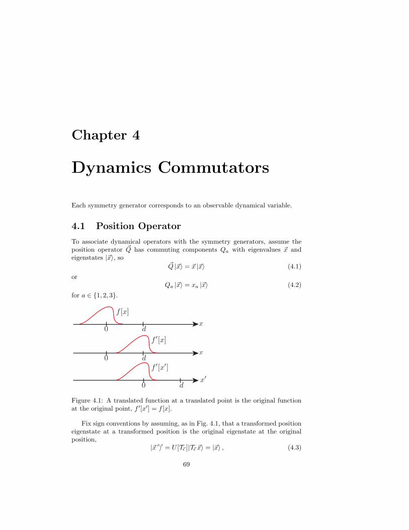
Chapter 4
Dynamics Commutators
Each symmetry generator corresponds to an observable dynamical variable.
4.1 Position Operator
To associate dynamical operators with the symmetry generators, assume theposition operator ~Q has commuting components Qa with eigenvalues ~x andeigenstates |~x〉, so
~Q |~x〉 = ~x |~x〉 (4.1)
orQa |~x〉 = xa |~x〉 (4.2)
for a ∈ {1, 2, 3}.
Figure 4.1: A translated function at a translated point is the original functionat the original point, f ′[x′] = f [x].
Fix sign conventions by assuming, as in Fig. 4.1, that a transformed positioneigenstate at a transformed position is the original eigenstate at the originalposition,
|~x ′〉′ = U [T~ε ]|T~ε ~x〉 = |~x〉 , (4.3)
69
Chapter 4. Dynamics Commutators 70
so thatU [T~ε ]|~x〉 =
∣∣T −1~ε ~x⟩. (4.4)
Consequently, the position eigenvalue Eq. 4.1 transforms as
U ~QU−1U |~x〉 = ~xU |~x〉 , (4.5a)
U ~QU−1∣∣T −1~ε ~x
⟩= ~x
∣∣T −1~ε ~x⟩, (4.5b)
~Q′ |~x〉 = T~ε ~x |~x〉 , (4.5c)
where the position operator transforms like
~Q′ = U [T~ε ] ~QU [T~ε ]−1 = U [T~ε ] ~QU [T~ε ]† = ei~ε·~T ′ ~Qe−i~ε·
~T ′ . (4.6)
For small transforms, to O[ε], this becomes
~Q′ =(
1 + i~ε · ~T ′)~Q(
1− i~ε · ~T ′)
= ~Q+ i~ε · ~T ′ ~Q− i ~Q~ε · ~T ′
= ~Q+ i[~ε · ~T ′, ~Q
], (4.7)
and the mixed commutator of a symmetry generator and a position operator
i[~ε · ~T ′, ~Q
]= ~Q′ − ~Q = T~ε ~xI − ~Q. (4.8)
4.1.1 Position and Space Translations
More specifically, under space translations,
S~ε ~x = ~x+ ~ε, (4.9)
the Eq. 4.1 position eigenvalue equation transforms as
U ~QU−1U |~x〉 = ~xU |~x〉 , (4.10a)
U ~QU−1∣∣S−1~ε ~x
⟩= ~x
∣∣S−1~ε ~x⟩, (4.10b)
~Q′ |~x〉 = S~ε ~x |~x〉= (~x+ ~ε) |~x〉
= ( ~Q+ ~ε I) |~x〉 , (4.10c)
Since the state |~x〉 is arbitrary,
~Q′ = ~Q+ ~ε I. (4.11)
But under space translations the position operator also transforms like
~Q′ = U [S~ε ] ~QU [S~ε ]−1 = ei~ε·~S′ ~Qe−i~ε·
~S′ , (4.12)
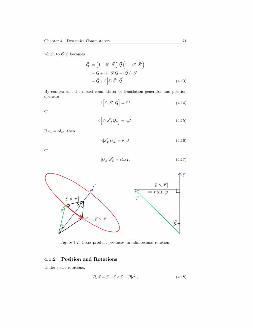
Chapter 4. Dynamics Commutators 71
which to O[ε] becomes
~Q′ =(
1 + i~ε · ~S′)~Q(
1− i~ε · ~S′)
= ~Q+ i~ε · ~S′ ~Q− i ~Q~ε · ~S′
= ~Q+ i[~ε · ~S′, ~Q
]. (4.13)
By comparison, the mixed commutator of translation generator and positionoperator
i[~ε · ~S′, ~Q
]= ~ε I (4.14)
or
i[~ε · ~S′, Qa
]= εaI. (4.15)
If εa = εδab, then
i[S′b, Qa] = δabI (4.16)
or
[Qa, S′b] = iδabI. (4.17)
Figure 4.2: Cross product produces an infinitesimal rotation.
4.1.2 Position and Rotations
Under space rotations,
R~ε ~x = ~x+ ~ε× ~x+O[ε2], (4.18)
Chapter 4. Dynamics Commutators 72
as in Fig. 4.2, the Eq. 4.1 position eigenvalue equation transforms as
U ~QU−1U |~x〉 = ~xU |~x〉 , (4.19a)
U ~QU−1∣∣R−1~ε ~x
⟩= ~x
∣∣R−1~ε ~x⟩, (4.19b)
~Q′ |~x〉 = R~ε ~x |~x〉= (~x+ ~ε× ~x) |~x〉
= ( ~Q+ ~ε× ~Q) |~x〉 , (4.19c)
Since the state |~x〉 is arbitrary,
~Q′ = ~Q+ ~ε× ~Q. (4.20)
But under space rotations the position operator also transforms like
~Q′ = U [R~ε ] ~QU [R~ε ]−1 = ei~ε·~R′ ~Qe−i~ε·
~R′ , (4.21)
which to O[ε] becomes
~Q′ =(
1 + i~ε · ~R′)~Q(
1− i~ε · ~R′)
= ~Q+ i~ε · ~R′ ~Q− i ~Q~ε · ~R′
= ~Q+ i[~ε · ~R′, ~Q
]. (4.22)
By comparison, the mixed commutator of rotation generator and position op-erator
i[~ε · ~R′, ~Q
]= ~ε× ~Q. (4.23)
Projecting on the vector ~v,
i[~ε · ~R′, ~v · ~Q
]= ~v · ~ε× ~Q. (4.24)
If ~ε = εxa and ~v = vxb, then
i[R′a, Qb] = xb · xa × ~Q = xb × xa · ~Q = −εabcxc · ~Q (4.25)
or
[R′a, Qb] = iεabcQc. (4.26)
4.1.3 Position and Boosts
Under velocity translations or boosts,
B~ε ~xt = ~xt + ~ε t, (4.27)
Chapter 4. Dynamics Commutators 73
the Eq. 4.1 position eigenvalue equation transforms as
U ~QU−1U |~xt〉 = ~xt U |~x〉 , (4.28a)
U ~QU−1∣∣B−1~ε ~xt
⟩= ~xt
∣∣B−1~ε ~xt⟩, (4.28b)
~Q′ |~xt〉 = B~ε ~xt |~xt〉= (~xt + ~ε t) |~xt〉
= ( ~Q+ ~ε tI) |~xt〉 , (4.28c)
Since the state |~xt〉 is arbitrary,
~Q′ = ~Q+ ~ε tI. (4.29)
But under boosts the position operator also transforms like
~Q′ = U [B~ε ] ~QU [B~ε ]−1 = ei~ε·~B′ ~Qe−i~ε·
~B′ , (4.30)
which to O[ε] becomes
~Q′ =(
1 + i~ε · ~B′)~Q(
1− i~ε · ~B′)
= ~Q+ i~ε · ~B′ ~Q− i ~Q~ε · ~B′
= ~Q+ i[~ε · ~B′, ~Q
]. (4.31)
By comparison, the mixed commutator of boost generator and position operator
i[~ε · ~B′, ~Q
]= ~ε tI (4.32)
or
i[~ε · ~B′, Qa
]= εatI. (4.33)
If ~ε = εδab, then
i[B′b, Qa] = δabtI (4.34)
or
[Qa, B′b] = iδabtI. (4.35)
Without loss of generality, at t = 0 there is no position change, and
[Qa, B′b] = 0, (4.36)
where U [B~ε] = exp[i~ε · ~B′] hereafter describes the instantaneous effects of avelocity translation or boost.

Chapter 4. Dynamics Commutators 74
4.1.4 Position and Time Translations
Nonrelativistic quantum mechanics does not treat time and space equally: time tis a parameter while space ~x is associated with the position operator ~Q. Hence,discovering the mixed commutator of the time translation generator and theposition operators requires a different technique.
Under time translations,Tε~xt = ~xt+ε, (4.37)
in order for the new state at the new time to be the old state at the old time,
|ψt′〉′ = U [Tε]∣∣ψTεt⟩ = |ψt〉. (4.38)
then the new state at the old time
|ψt〉′ = eiεT′|ψt〉 = U [Tε]|ψt〉 =
∣∣ψT−1ε t
⟩= |ψt−ε〉. (4.39)
If ε = t, theneitT
′|ψt〉 = |ψ0〉. (4.40)
and|ψt〉 = e−itT
′|ψ0〉. (4.41)
Differentiate both sides with respect to the time t parameter to find
|ψt+dt〉 − |ψt〉dt
=d
dt|ψt〉 = −iT ′|ψt〉 (4.42)
and its adjoint〈ψt+dt| − 〈ψt|
dt=
d
dt〈ψt| = 〈ψt|iT ′. (4.43)
4.2 Velocity Operator
Introduce the velocity operator by the classical correspondence of expectationvalues ⟨
~V⟩
=d
dt
⟨~Q⟩
(4.44)
or, more explicitly,⟨ψt
∣∣∣~V ∣∣∣ψt⟩ =d
dt
⟨ψt
∣∣∣ ~Q∣∣∣ψt⟩=
(d
dt〈ψt|
)~Q |ψt〉+ 〈ψt| ~Q
(d
dt|ψt〉
)= 〈ψt| iT ′ ~Q |ψt〉 − 〈ψt| i ~QT ′ |ψt〉
= 〈ψt| i[T ′, ~Q
]|ψt〉 . (4.45)

Chapter 4. Dynamics Commutators 75
Since this is true for all state vectors,
~V = i[T ′, ~Q
](4.46)
or
[Qa, T′] = iVa. (4.47)
Compute the mixed commutators of the velocity operator with the sym-metry generators using the Section 4.1 position operator techniques or by theantisymmetry of the existing commutators. For example,[
~ε · ~B′, Vb]
= εa[B′a, Vb]
= −iεa[B′a, [Qb, T′]]
= iεa([T ′, [B′a, Qb]] + [Qb, [T
′, B′a]])
= iεa([T ′, 0]− i[Qb, S′a]
)= iεa(0 + δbaI)
= iεbI (4.48)
with ~ε = εxa implies
[B′a, Vb] = iδabI. (4.49)
Note that the boost of the velocity operator is
U [B~ε]~V U [B~ε]−1 = ei~ε·
~B′ ~V e−i~ε·~B′
=(
1 + i~ε · ~B′)~V(
1− i~ε · ~B′)
= ~V + i~ε · ~B′ ~V − i~V ~ε · ~B′
= ~V + i[~ε · ~B′, ~V
]= ~V − ~ε I (4.50)
to O[ε] (and by Eq. 4.113, this is true to all orders of ε). As a consequence, theoperator transformation
~V ′ = ei~ε·~B′ ~V e−i~ε·
~B′ = ~V − ~ε I, (4.51)
which is plausible, as boosts are velocity translations.
Table 4.1 summarizes the commutations relations of the position and velocityoperators with the Galilei symmetry generators for free particles, while Table 4.2summarizes the infinitesimal transformations of states and observables.
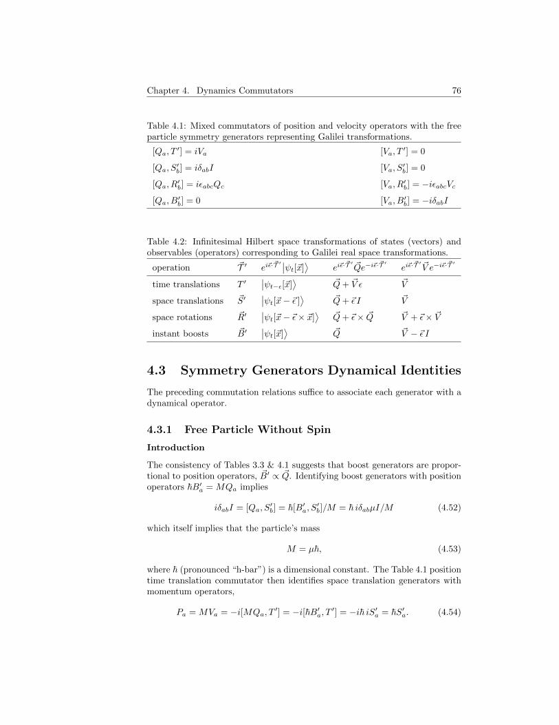
Chapter 4. Dynamics Commutators 76
Table 4.1: Mixed commutators of position and velocity operators with the freeparticle symmetry generators representing Galilei transformations.
[Qa, T′] = iVa [Va, T
′] = 0
[Qa, S′b] = iδabI [Va, S
′b] = 0
[Qa, R′b] = iεabcQc [Va, R
′b] = −iεabcVc
[Qa, B′b] = 0 [Va, B
′b] = −iδabI
Table 4.2: Infinitesimal Hilbert space transformations of states (vectors) andobservables (operators) corresponding to Galilei real space transformations.
operation ~T ′ ei~ε·~T ′∣∣ψt[~x]
⟩ei~ε·
~T ′ ~Qe−i~ε·~T ′ ei~ε·
~T ′ ~V e−i~ε·~T ′
time translations T ′∣∣ψt−ε[~x]
⟩~Q+ ~V ε ~V
space translations ~S′∣∣ψt[~x− ~ε ]
⟩~Q+ ~ε I ~V
space rotations ~R′∣∣ψt[~x− ~ε× ~x]
⟩~Q+ ~ε× ~Q ~V + ~ε× ~V
instant boosts ~B′∣∣ψt[~x]
⟩~Q ~V − ~ε I
4.3 Symmetry Generators Dynamical Identities
The preceding commutation relations suffice to associate each generator with adynamical operator.
4.3.1 Free Particle Without Spin
Introduction
The consistency of Tables 3.3 & 4.1 suggests that boost generators are propor-tional to position operators, ~B′ ∝ ~Q. Identifying boost generators with positionoperators ~B′a = MQa implies
iδabI = [Qa, S′b] = ~[B′a, S
′b]/M = ~ iδabµI/M (4.52)
which itself implies that the particle’s mass
M = µ~, (4.53)
where ~ (pronounced “h-bar”) is a dimensional constant. The Table 4.1 positiontime translation commutator then identifies space translation generators withmomentum operators,
Pa = MVa = −i[MQa, T′] = −i[~B′a, T ′] = −i~ iS′a = ~S′a. (4.54)

Chapter 4. Dynamics Commutators 77
This obvious first identification,
~ ~B′ = M ~Q ≡ ~C, (4.55a)
~~S′ = M~V ≡ ~P , (4.55b)
and Table 4.1 implies the famous position-momentum commutator
[Qa, Pb] = i~δabI, (4.56)
which implies (in popular notation)
[X,Px] = i~. (4.57)
Irreducible Sets
For a particle with no internal degrees of freedom, the position and momentumoperators { ~Q, ~P} are irreducible: if an operator commutes with ~Q, it cannot be
a function of ~P , and if it commutes with ~P , it cannot be a function of ~Q, andif it commutes with both ~Q and ~P , it must be a constant. This is plausiblephysically, as classical Hamiltonian dynamics uniquely determines orbits basedon single initial points in position-momentum “phase space”. The Eq. 4.55identification thus implies that the generators of velocity and space translations{ ~B′, ~S′} are also irreducible.
Position
Assuming { ~B′, ~S′} irreducibility, check that the identification of boost genera-
tors with position operators is unique by noting that since ~ ~B′−M ~Q commuteswith space translation generators ~S′,
[~B′a −MQa, S′b] = ~[B′a, S
′b]−M [Qa, S
′b]
=����~ iδabµI −����MiδabI = 0, (4.58)
assuming M = µ~, it cannot be a function of ~S′. Since it commutes with velocitytranslation generators ~B′,
[~B′a −MQa, B′b] = ~[B′a, B
′b]−M [Qa, B
′b] = 0− 0 = 0, (4.59)
it cannot be a function of ~B′. Thus, if there are no internal degrees of freedom,it must be a constant,
~ ~B′ −M ~Qa = ~kI. (4.60)
But from Table 4.1,
[R′a, Qb] = iεabcQc, (4.61a)
[R′a,MQb] = iεabcMQc, (4.61b)
[R′a, ~B′b − kbI] = iεabc(~B′c − kcI), (4.61c)
�����~[R′a, B′b] =��
���~ iεabcB′c − iεabckcI, (4.61d)
so the constant ~k = ~0.

Chapter 4. Dynamics Commutators 78
Linear Momentum
Still assuming { ~B′, ~S′} irreducibility, check that the identification of space trans-lation generators with momentum operators is unique by noting that since~~S′ − ~P commutes with space translation generators ~S′,
[~S′a − Pa, S′b] = ~[S′a, S′b]−M [Va, S
′b] = 0− 0 = 0, (4.62)
it cannot be a function of ~S′. Since it commutes with velocity translationgenerators ~B′,
[~S′a − Pa, B′b] = ~[S′a, B′b]−M [Va, B
′b] = ~(−iδabµI) +M i~δabI = 0, (4.63)
as M = µ~, it cannot be a function of ~B′. Thus, if there are no internal degreesof freedom, it must be a constant,
~~S′ − ~P = ~kI. (4.64)
But from Table 4.1,
iεabcS′c = [R′a, S
′b], (4.65a)
iεabc~S′c = [R′a, ~S′b], (4.65b)
iεabc(MVc + kcI) = [R′a,MVb + kbI], (4.65c)
�����iεabcMVc + iεabckcI = M [R′a, Vb],
= −iM [R′a, [Qb, T′]]
= iM([T ′, [R′a, Qb]] + [Qb, [T′, R′a]])
= −εabcM([T ′, Qc] + [Qb, 0])
=�����iεabcMVc , (4.65d)
so the constant ~k = ~0.
Angular Momentum
Furthermore, identifying rotation generators with angular momenta operators~R′a = εabcQbPc = Lc implies
����[R′a, B′b] = εacd[QcPd, B
′b]/~
= εacd[B′cS′d, B
′b]~/M
= εacd(B′c[S′d, B
′b] + [B′c, B
′b]S′d)~/M
= εacd(−iδbdµB′c + 0)~/M= −iεacbB′c=���
�iεabcB′c , (4.66)
Chapter 4. Dynamics Commutators 79
and similarly for the other Table 3.3 blue commutators. Now { ~B′, ~S′} irre-
ducibility implies { ~Q, ~P} irreducibility, so check that this identification is nec-
essary by noting that since ~R′a − εabcQbPc commutes with momentum ~P ,
[~R′a − εabcQbPc, Pb] = ~[R′a, Pb]− εabc[QbPc, Pb]= ~2[R′a, S
′b]− εabc(Qb[Pc, Pb] + [Qb, Pb]Pc)
= ~2iεabcS′c − εabci~Pc = 0, (4.67)
it cannot be a function of ~P . Since it commutes with position ~Q,
[~R′a − εabcQbPc, Qb] = ~[R′a, Qb]− iεabc[QbPc, Qb]= ~iεabcQc − iεabc(Qb[Pc, Qb] + [Qb, Qb]Pc)
= −~iεabcQb + εabci~Qb = 0, (4.68)
it cannot be a function of ~Q. Thus, if there are no internal degrees of freedom,it must be a constant,
~R′a − εabcQbPc = kaI. (4.69)
But from Tables 3.3 & 4.1 and the Eq. 4.111b identity,
[R′a, R′b] = iεabcR
′c,
[~R′a, R′b] = iεabc~R′c,[εacdQcPd + kaI,R
′b] = iεabc(εcdeQdPe + kcI),
εacd~2[B′cS′d, R
′b] = iεabc~2(εcdeB
′dS′e +MkcI),
εacd(B′c[S′d, R
′b] + [B′c, R
′b]S′d) = iεabcεcdeB
′dS′e + iεabcMkc/I~2,
εacd(−iεbdeB′cS′e − iεbceB′eS′d) = i(δadδbe − δaeδbd)B′dS′e + iεabcMkcI/~2,εdacεdbeB
′cS′e − εcadεcbeB′eS′d = (δadδbe − δaeδbd)B′dS′e + εabcMkcI/~2,
(δabδce − δaeδcb)B′cS′e − (δabδde − δaeδdb)B′eS′d = B′aS′b −B′bS′a + εabcMkcI/~2,
�����
δab ~B′ · ~S ′ −HHHB′bS
′a −���
��δab ~B
′ · ~S ′ +���B′aS′b =��
�B′aS′b −HHHB′bS
′a + εabcMkcI/~2,
0 = εabcMkcI/~2, (4.70)
so the constant ~k = ~0.
Energy
Finally, identifying time translation generators with the energy operator ~T ′ =PaPa/2M = H implies
����[B′a, T′] = [B′a, PbPb]/2M~
= [B′a, S′bS′b]~/2M
= (S′b[B′a, S
′b] + [B′a, S
′b]S′b)~/2M
= (S′b iδabµI + iδabµI S′b)~/2M
=��iS′a . (4.71)
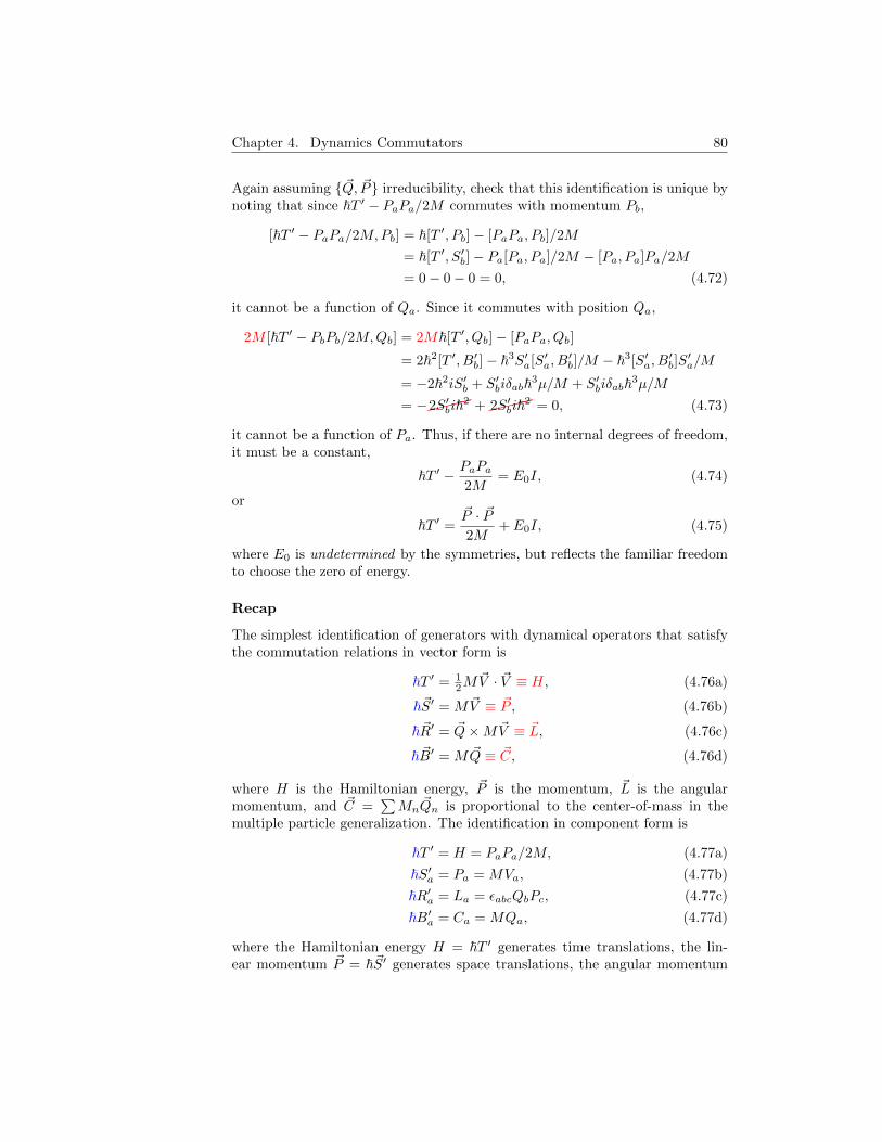
Chapter 4. Dynamics Commutators 80
Again assuming { ~Q, ~P} irreducibility, check that this identification is unique bynoting that since ~T ′ − PaPa/2M commutes with momentum Pb,
[~T ′ − PaPa/2M,Pb] = ~[T ′, Pb]− [PaPa, Pb]/2M
= ~[T ′, S′b]− Pa[Pa, Pa]/2M − [Pa, Pa]Pa/2M
= 0− 0− 0 = 0, (4.72)
it cannot be a function of Qa. Since it commutes with position Qa,
2M [~T ′ − PbPb/2M,Qb] = 2M~[T ′, Qb]− [PaPa, Qb]
= 2~2[T ′, B′b]− ~3S′a[S′a, B′b]/M − ~3[S′a, B
′b]S′a/M
= −2~2iS′b + S′biδab~3µ/M + S′biδab~3µ/M= −����2S′bi~2 +���
�2S′bi~2 = 0, (4.73)
it cannot be a function of Pa. Thus, if there are no internal degrees of freedom,it must be a constant,
~T ′ − PaPa2M
= E0I, (4.74)
or
~T ′ =~P · ~P2M
+ E0I, (4.75)
where E0 is undetermined by the symmetries, but reflects the familiar freedomto choose the zero of energy.
Recap
The simplest identification of generators with dynamical operators that satisfythe commutation relations in vector form is
~T ′ = 12M
~V · ~V ≡ H, (4.76a)
~~S′ = M~V ≡ ~P , (4.76b)
~~R′ = ~Q×M~V ≡ ~L, (4.76c)
~ ~B′ = M ~Q ≡ ~C, (4.76d)
where H is the Hamiltonian energy, ~P is the momentum, ~L is the angularmomentum, and ~C =
∑Mn
~Qn is proportional to the center-of-mass in themultiple particle generalization. The identification in component form is
~T ′ = H = PaPa/2M, (4.77a)
~S′a = Pa = MVa, (4.77b)
~R′a = La = εabcQbPc, (4.77c)
~B′a = Ca = MQa, (4.77d)
where the Hamiltonian energy H = ~T ′ generates time translations, the lin-ear momentum ~P = ~~S′ generates space translations, the angular momentum
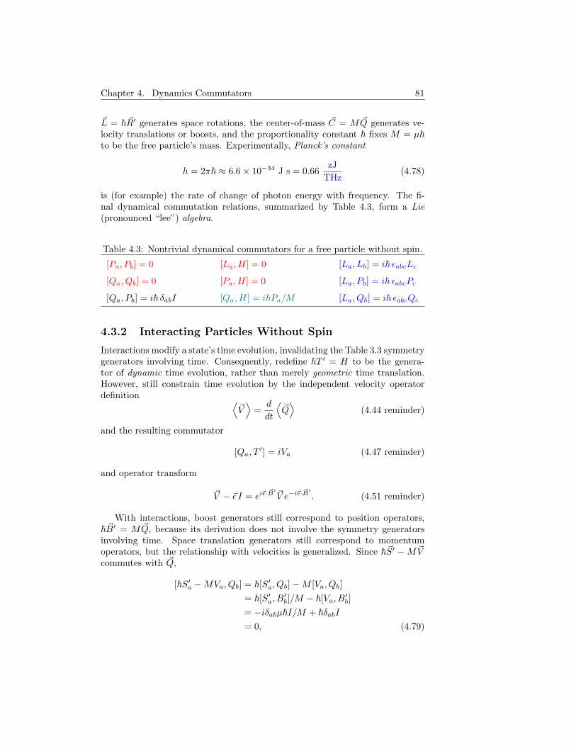
Chapter 4. Dynamics Commutators 81
~L = ~~R′ generates space rotations, the center-of-mass ~C = M ~Q generates ve-locity translations or boosts, and the proportionality constant ~ fixes M = µ~to be the free particle’s mass. Experimentally, Planck’s constant
h = 2π~ ≈ 6.6× 10⁻³⁴ J s = 0.66zJ
THz(4.78)
is (for example) the rate of change of photon energy with frequency. The fi-nal dynamical commutation relations, summarized by Table 4.3, form a Lie(pronounced “lee”) algebra.
Table 4.3: Nontrivial dynamical commutators for a free particle without spin.
[Pa, Pb] = 0 [La, H] = 0 [La, Lb] = i~ εabcLc[Qa, Qb] = 0 [Pa, H] = 0 [La, Pb] = i~ εabcPc[Qa, Pb] = i~ δabI [Qa, H] = i~Pa/M [La, Qb] = i~ εabcQc
4.3.2 Interacting Particles Without Spin
Interactions modify a state’s time evolution, invalidating the Table 3.3 symmetrygenerators involving time. Consequently, redefine ~T ′ = H to be the genera-tor of dynamic time evolution, rather than merely geometric time translation.However, still constrain time evolution by the independent velocity operatordefinition ⟨
~V⟩
=d
dt
⟨~Q⟩
(4.44 reminder)
and the resulting commutator
[Qa, T′] = iVa (4.47 reminder)
and operator transform
~V − ~ε I = ei~ε·~B′ ~V e−i~ε·
~B′ . (4.51 reminder)
With interactions, boost generators still correspond to position operators,~ ~B′ = M ~Q, because its derivation does not involve the symmetry generatorsinvolving time. Space translation generators still correspond to momentumoperators, but the relationship with velocities is generalized. Since ~~S′ −M~Vcommutes with ~Q,
[~S′a −MVa, Qb] = ~[S′a, Qb]−M [Va, Qb]
= ~[S′a, B′b]/M − ~[Va, B
′b]
= −iδabµ~I/M + ~δabI= 0, (4.79)
Chapter 4. Dynamics Commutators 82
and there are no internal degrees of freedom, it must be a function of ~Q,
~~S′ −M~V = ~A[~Q]
(4.80)
or~P ≡ ~~S′ = M~V + ~A
[~Q], (4.81)
where ~A represents momentum stored in the interacting fields.
Similarly, the time translation generator still corresponds to the Hamiltonianenergy operator but in a generalized way. Since ~A and ~Q commute, identifyingtime translation generators with the energy operator
~H ≡ ~T ′ =(~P − ~A
)2/2M (4.82)
implies
XXXXi[H,Qa] = i[(Pb −Qb)(Pb −Qb), Qa]/2M
= i ([PbPb, Qa]− [PbAb, Qa]− [AbPb, Qa] + [AbAb, Qa]) /2M
= i (Pb [Pb, Qa] + [Pb, Qa]Pb − [Pb, Qa]Ab −Ab [Pb, Qa] + 0) /2M
= i (−Pb i~δab − i~δabPb + i~δabAb +Ab i~δab) /2M= (Pa −Aa)/M
=ZZVa . (4.83)
However, this identification is not unique, as adding or subtracting any functionof position V
[~Q]
also works. With the most general identification allowed by theGalilei group of symmetry transformations, external fields shift the free energyand linear momentum operators by functions of position, so
H − V[~Q]
=1
2M
(~P − ~A
[~Q])2
. (4.84)
4.3.3 Free Particle With Spin
The internal degrees of freedom are independent of position ~Q and momentum~P . In particular, spin degrees of freedom generalize the relation between spacerotation generators and angular momentum operators to
~J = ~L+ ~S , (4.85)
where the spin angular momentum operators satisfy
[Sa,Sb] = iεabcSc, (4.86)
and S is pronounced “big script s”. The other identifications proceed similarly.
Chapter 4. Dynamics Commutators 83
4.4 Position Space Schrodinger Equation
Assuming a time translated state at a time translated instant is the originalstate at the original instant,
|ψ′t〉′ = U [Tε]|ψTεt〉 = |ψt〉 , (4.87)
the infinitesimal time translation of a generic state
eiεH/~|ψt〉 = eiεT′|ψt〉 = U [Tε]|ψt〉 =
∣∣ψT−1ε t
⟩=∣∣ψt−ε⟩ (4.88)
or ∣∣ψt−ε⟩ = eiεH/~|ψt〉, (4.89)
To O[ε], ∣∣ψt−ε⟩ =
(1 + iε
H
~
)|ψt〉 (4.90)
implies the differential equation
− iH~|ψt〉 =
|ψt〉 − |ψt−ε〉ε
=∂
∂t|ψt〉 (4.91)
or
H |ψt〉 = i~ ∂t |ψt〉 , (4.92)
which is the state space Schrodinger equation. Since the state |ψt〉 is arbitrary,the Hamiltonian energy operator acts like the time derivative
H = +i~ ∂t. (4.93)
Assuming a space translated position eigenstate at a space translated posi-tion is the original eigenstate at the original position,
|~x ′〉′ = U [S~ε]|S~ε ~x〉 = |~x〉 , (4.94)
the infinitesimal space translation of a position eigenstate
ei~ε·~P/~|~x〉 = ei~ε·
~S′ |~x〉 = U [S~ε]|~x〉 = |S−1~ε ~x〉 = |~x− ~ε 〉. (4.95)
and its adjoint
〈~x− ~ε | = 〈~x|e−i~ε·~P/~ (4.96)
projected onto a generic state
〈~x− ~ε |ψt〉 = 〈~x|e−i~ε·~P/~|ψt〉 (4.97)
or
ψt[~x− ~ε ] = e−i~ε·~P/~ψt[~x], (4.98)
Chapter 4. Dynamics Commutators 84
where the operators Pa on state space and the corresponding operators Πa onwave function space are identified Pa ↔ Πa by 〈~x|Pa|ψt〉 = Πa〈~x|ψt〉. To O[ε],
ψt[~x− ~ε ] =
(1− i~ε ·
~P
~
)ψt[~x] (4.99)
implies the differential equation
iε ·~P
~ψt[~x] =
ψt[~x]− ψt[~x− ~ε ]
ε= ε · ~∇ψt[~x]. (4.100)
Since the direction ε is arbitrary,
~Pψt[~x] = −i~~∇ψt[~x], (4.101)
and since the wave function ψt[~x] is arbitrary, the position representation of themomentum operator acts like the space derivative or gradient
~P = −i~~∇. (4.102)
The position operator definition
~Q|~x〉 = ~x|~x〉 (4.103)
and its adjoint〈~x| ~Q = 〈~x|~x (4.104)
projected onto a generic state
〈~x| ~Q|ψt〉 = 〈~x|~x|ψt〉 (4.105)
implies~Qψt[~x] = ~xψt[~x], (4.106)
where again state and wave function operators are identified Qa ↔ Θa by〈~x|Qa|ψt〉 = Θa〈~x|ψt〉. Since the wave function ψt[~x] is arbitrary, the positionrepresentation of the position operator (unsurprisingly) acts like multiplicationby position
~Q = ~x. (4.107)
Finally, “sandwich” the ~A = ~0 Eq. 4.84 Hamiltonian
H =1
2M~P · ~P + V
[~Q]
(4.108)
between the position eigenstate 〈~x| and the state |ψt〉 to write
〈~x|H|ψt〉 =⟨~x∣∣ 12M
~P · ~P + V[~Q]∣∣ψt⟩ (4.109)
and use the Eq. 4.93, Eq. 4.102, and Eq. 4.107 position representations to writethe position space Schrodinger equation
i~ ∂tψt[~x] = − ~2
2M∇2ψt[~x] + V[~x]ψt[~x]. (4.110)
Chapter 4. Dynamics Commutators 85
Problems
1. Prove the following ε-δ identities, with implied sums over repeated indices,
εabcεmno = det
δam δan δao
δbm δbn δbo
δcm δcn δco
= +δamδbnδco + δaoδbmδcn + δanδboδcm
− δamδboδcn − δanδbmδco − δaoδbnδcm, (4.111a)
εsabεsmn = δamδbn − δanδbm, (4.111b)
εrsaεrsm = 2δam, (4.111c)
εrstεrst = 6, (4.111d)
and use one of them to prove the “bac-cab” identity
~a×(~b× ~c
)= ~b(~a · ~c
)− ~c(~a ·~b
). (4.112)
2. Prove that [Ua, Ub] = iεabcWc is equivalent to ~U × ~U = i ~W .
3. If A and B are operators and x is a parameter, prove that
exABe−xA = B + [A,B]x+1
2![A, [A,B]]x2 +
1
3![A, [A, [A,B]]]x3 + · · · .
(4.113)(Hint: If f [x] = exABe−xA, then show df/dx = [A, f ], and so on.)
4. Use Eq. 4.113 to verify the Table 4.2 operator transformations.
5. Substitute the Eq. 4.76 identifications into the Table 4.1 mixed commuta-tors, and show they are consistent with the Table 4.3 final commutators.
6. Compare and contrast the hermitian boost generators ~B′ and
~ ~B′ = M ~Q− t ~P . (4.114)
In particular, use Eq. 4.113 to compute the effects of the correspondingunitary transformations on the position and momentum operators ~Q and~P . Why are boosts also known as velocity translations?
7. Prove the Eq. 4.57 position-momentum commutator in the position basisusing the Eq. 4.102 momentum operator representation. (Hint: Apply thecommutator to the generic wave function ψt[x] and use calculus.)
8. By Eq. 4.102, the momentum acts like a derivative in the position basis,
〈x|Px|ψ〉 = −i~ ∂xψ[x] = −i~ ∂x〈x|ψ〉. (4.115)

Chapter 4. Dynamics Commutators 86
(a) Consider |ψ〉 = |p〉 to be a state of definite momentum Px|p〉 = p|p〉and solve
〈x|Px|p〉 = −i~ ∂x〈x|p〉 (4.116)
to find〈x|p〉 = Ceipx/~. (4.117)
(b) To find the constant C, use the orthonormalization 〈p|p′〉 = δ[p−p′],the resolution of the identity I =
∫dx |x〉〈x|, and the Dirac delta
representation δ[p] =∫dx eipx/~/(2π~).
(c) Use the state expansion
|ψ〉 = I|ψ〉 =
∫dx |x〉〈x|ψ〉 (4.118)
to show that the position wave functions ψ[x] = 〈x|ψ〉 are the Fouriertransforms of the momentum wave functions ψ[p] = 〈p|ψ〉.
Chapter 5
Harmonic Oscillator
The harmonic oscillator is the most important model system in both classicaland quantum physics.
5.1 Classical Harmonic Oscillator
Consider a simple (or ideal) harmonic oscillator, a mass m connected to aHooke’s law spring of stiffness k. If the displacement is x, then the linearrestoring force is Fx = −kx, and the quadratic (or parabolic) potential energyfunction is
V [x] =1
2kx2. (5.1)
The equation of motion follows from Newton’s second law ax = Fx/m, namely
x = ∂2t x = − 1
m∂xV = − 1
mV ′[x] = − k
mx. (5.2)
This has the well-known sinusoidal solution
x[t] = A sin[ωt+ ϕ], (5.3)
provided the angular frequency ω =√k/m. The constants A and ϕ depend on
the initial conditions. In phase space {x, px}, energy
E =1
2mv2x + V [x] =
1
2mp2x +
mω2
2x2 (5.4)
conservation implies elliptical orbits.Real springs, of course, aren’t so simple. Stretch them too far, for example,
and they break. However, almost any potential energy function is approximatelyparabolic near a local minimum. If the potential V [x] has a minimum at x0,expand in a Taylor series to get
V [x] = V [x0] + V ′[x0] (x− x0) +1
2V ′′[x0](x− x0)
2+ · · · . (5.5)
87
Chapter 5. Harmonic Oscillator 88
Since V ′[x0] = 0, near x0
V [x]− V [x0] ∼ 1
2V ′′[x0](x− x0)
2(5.6)
or
δV ∼ 1
2k(δx)
2, (5.7)
where k = V ′′[x0]. Thus, the simple harmonic oscillator is a canonical systemof widespread importance.
5.2 Commutator Solution
Quantum mechanically, the Eq. 5.4 harmonic oscillator oscillator implies theHamiltonian operator
H =1
2mP 2 +
mω2
2Q2, (5.8)
where the energy spectrum of H follows algebraically from the Table 4.3 com-mutation relation
[Q,P ] = i~I, (5.9)
and the hermeticity of the position and momentum operators.
5.2.1 Dimensionless Variables
An oscillator of energy
1
2~ω =
1
2mp2x +
mω2
2x2 =
1
2mp20 + 0 = 0 +
mω2
2x20 (5.10)
defines a maximum position x0 =√~/mω and momentum p0 =
√m~ω, which
define dimensionless operators
q =Q
x0=
√mω
~Q, (5.11a)
p =P
p0=
√1
m~ωP, (5.11b)
so that
[q, p] =
[√mω
~Q,
√1
m~ωP
]=
1
~[Q,P ] = i, (5.12)
where the identity operator I is implicit in the final step, as is conventional.The Eq. 5.8 Hamiltonian becomes
H =1
2m
(m~ω p2
)+mω2
2
(~mω
q2)
=1
2~ω(p2 + q2
). (5.13)

Chapter 5. Harmonic Oscillator 89
5.2.2 Creation & Annihilation Operators
Introduce creation and annihilation operators
a =q + ip√
2, (5.14a)
a† =q − ip√
2, (5.14b)
such that
q =a+ a†√
2, (5.15a)
p =a− a†
i√
2, (5.15b)
and
[a, a†] =1
2
([q, q]− i[q, p] + i[p, q] + [p, p]
)= −i[q, p] = 1. (5.16)
Substitute the Eq. 5.15 dimensionless operators into the Eq. 5.119 Hamiltonianto “factorize” it into
H =1
2~ω(−(a− a†)2 + (a+ a†)2
2
)=
1
2~ω(aa† + a†a
)= ~ω
(a†a+
1
2
)= ~ω
(N +
1
2
), (5.17)
where the hermitian number operator
N = a†a = (a†a)† = N† (5.18)
obeys
[N, a] = [a†a, a] = a†[a, a] + [a†, a]a = −a, (5.19a)
[N, a†] = [a†a, a†] = a†[a, a†] + [a†, a†]a = +a†. (5.19b)
5.2.3 Number Operator Spectrum
Let |λ〉 be an eigenstate of the number operator N with eigenvalue λ so that
N |λ〉 = λ|λ〉. (5.20)

Chapter 5. Harmonic Oscillator 90
First “annihilate” or “lower” an eigenstate to a|λ〉 and apply the number oper-ator
Na|λ〉 = (aN + [N, a])|λ〉 = (aN − a)|λ〉 = (aλ− a)|λ〉 = (λ− 1)a|λ〉 (5.21)
to show thata|λ〉 ∝ |λ− 1〉 (5.22)
is an eigenstate with eigenvalue λ− 1,
N |λ− 1〉 = (λ− 1)|λ− 1〉. (5.23)
Similarly, show thata2|λ− 2〉 ∝ |λ− 2〉 (5.24)
is an eigenstate with eigenvalue λ− 2,
N |λ− 2〉 = (λ− 2)|λ− 2〉. (5.25)
Continue to create a downward “ladder” of eigenstates and eigenvalues. Theladder must have a bottom rung, because if |µ〉 = a|λ〉, then
0 ≤ 〈µ|µ〉 = 〈λ|a†a|λ〉 = 〈λ|N |λ〉 = λ〈λ|λ〉 = λ (5.26)
must be nonnegative. Let |ψ〉 = |0〉 be the vacuum state such that
a|0〉 = 0, (5.27)
so that further annihilations will produce no more eigenstates. Normalize theannihilation operator such that
a|n〉 = cn|n− 1〉, (5.28)
wheren = 〈n|N |n〉 = 〈n|a†a|n〉 = 〈n− 1|c∗ncn|n− 1〉 = |cn|2. (5.29)
Choose a real and positive normalization cn =√n so that
a|n〉 =√n|n− 1〉. (5.30)
Next “create” or “raise” an eigenstate to a†|λ〉 and apply the number oper-ator
Na†|λ〉 = (a†N + a†)|λ〉 = (a†λ+ a†)|λ〉 = (λ+ 1)a†|λ〉 (5.31)
to show thata†|λ〉 ∝ |λ+ 1〉 (5.32)
is an eigenstate with eigenvalue λ+ 1,
N |λ+ 1〉 = (λ+ 1)|λ+ 1〉. (5.33)
Similarly, show that(a†)2|λ+ 2〉 ∝ |λ+ 2〉 (5.34)

Chapter 5. Harmonic Oscillator 91
is an eigenstate with eigenvalue λ+ 2,
N |λ+ 2〉 = (λ+ 2)|λ+ 2〉. (5.35)
Continue to create an upward “ladder” of eigenstates and eigenvalues. Theladder does not have a top rung. Normalize the creation operator by
a†|n〉 =√n+ 1|n+ 1〉. (5.36)
5.2.4 Energy Spectrum
Thus, the orthonormal eigenstates of the number operator satisfy
N |n〉 = n|n〉 (5.37)
for nonnegative integers n = 0, 1, 2, . . ., and by Eq. 5.17, the orthonormal eigen-states of the Hamiltonian operator satisfy
H|En〉 = En|En〉, (5.38)
where
En =
(n+
1
2
)~ω. (5.39)
The ground state or zero-point energy E0 = ~ω/2 is nonzero due to theHeisenberg uncertainty principle. If it were zero, the oscillator’s position andmomentum would be both be exactly zero, but if one of the two is exact, theother must be indeterminate. The zero-point energy of the quantum vacuummay be related to the Dark Energy (or Clear Tension) that seems to be accel-erating the expansion of the universe.
The regular energy spacing ∆E = En+1−En = ~ω makes possible the pho-ton model of light. Transitions between adjacent energy levels are accompaniedby the emission or absorption of photons of energy ~ω, corresponding to classicallight of temporal frequency ω.
5.2.5 Wave Functions
The harmonic oscillator wave functions
ψn[x] = 〈x|n〉 (5.40)
are the projections of the eigenstates |n〉 in the position basis. For example, findthe ground state wave function by projecting the vacuum state annihilation
0 = a|0〉 =q + ip√
2|0〉 =
1√2
(√mω
~Q+ i
√1
m~ωP
)|0〉 (5.41)
on the position basis
0 =
√mω
~〈x|Q|0〉+ i
√1
m~ω〈x|P |0〉 =
√mω
~xψ0[x] + i
√1
m~ω(−i~∂xψ0[x])
(5.42)
Chapter 5. Harmonic Oscillator 92
using the Eq. 4.107 and Eq. 4.102 representations for the position and momen-tum operators in the position basis to get the differential equation
− mω
~xψ0 =
dψ
dx. (5.43)
Separate variables
− mω
~xdx =
dψ
ψ0(5.44)
and integrate
− mω
~x2
2= logψ0 − logN0 (5.45)
to find the gaussian ground state wave function
ψ0[x] = N0e−mωx2/2~ = N0e
− 12 (x/x0)
2
, (5.46)
where N0 is a normalization constant.
5.3 Differential Equation Solution
An alternate approach to finding the spectrum of the quantum harmonic oscil-lator is to solve the eigenvalue problem
H|E〉 = E|E〉 (5.47)
for the Eq. 5.8 Hamiltonian in the position basis
〈x|H|E〉 = E〈x|E〉, (5.48)
which implies the differential equation
1
2m(−i~∂x)2ψE [x] +
mω2
2x2ψE [x] = EψE [x] (5.49)
or
− ~2
2mψ′′ +
mω2
2ψ = Eψ, (5.50)
where ψ = ψE [x] ∈ R is real for simplicity, subject to the normalization con-straint
1 = 〈E|E〉 =
∫dx 〈E|x〉〈E|x〉 =
∫ ∞−∞
dxψE [x]∗ψE [x] =
∫ ∞−∞
dxψ2. (5.51)
This famous problem is nontrivial.

Chapter 5. Harmonic Oscillator 93
5.3.1 Dimensionless Variables
Again introduce dimensionless variables. For the position scale, let x0 be theclassical turning point for a harmonic oscillator with energy E0 = ~ω/2. Thus
1
2~ω = E0 =
1
2mv2 +
1
2kx2 = 0 +
1
2kx20, (5.52)
which implies
x0 =
√~ωk
=
√~mω
. (5.53)
Use this scale to define a dimensionless position
ξ =x
x0(5.54)
and a dimensionless eigenfunction
ϕ[ξ] =√x0ψ[x]. (5.55)
Then the derivatives transform like
ψ′ =dψ
dx=
1√x0
dϕ
dx=
1√x0
dξ
dx
dϕ
dξ=
1
x03/2ϕ′ (5.56)
and
ψ′′ =dψ′
dx=
1
x03/2dϕ′
dx=
1
x03/2dξ
dx
dϕ′
dξ=
1
x05/2ϕ′′, (5.57)
where, as usual, the prime denotes derivative with respect to the argument (x orξ, as appropriate). Putting this altogether, our problem transforms to solving
ϕ′′ =(ξ2 − ε
)ϕ (5.58)
subject to the constraint
1 =
∫ ∞−∞
dξ ϕ2, (5.59)
where the dimensionless energy
ε =E
E0. (5.60)
5.3.2 Asymptotic Behavior
When ξ is large, neglect ε and write
ϕ′′ ∼ ξ2ϕ, (5.61)
which has the approximate exponential solutions
ϕ ∼ ±e± 12 ξ
2
. (5.62)
Chapter 5. Harmonic Oscillator 94
To verify this, note that
ϕ′ ∼ ξe± 12 ξ
2
(5.63)
andϕ′′ ∼
(±1 + ξ2
)e±
12 ξ
2
∼ ξ2ϕ. (5.64)
Since only the decaying exponential is square normalizable, strip off theasymptotic behavior by assuming solutions of the form
ϕ[ξ] = h[ξ]e−12 ξ
2
, (5.65)
and expect the functions h[ξ] to be polynomials. Then
ϕ′ = (h′ − ξh) e−12 ξ
2
(5.66)
andϕ′′ =
(h′′ − 2ξh′ +
(ξ2 − 1
)h)e−
12 ξ
2
. (5.67)
With these substitutions, the exponentials cancel, and our differential equationbecomes
h′′ − 2ξh′ + (ε− 1)h = 0. (5.68)
5.3.3 Power Series Solution
Write the solution as a power series
h[ξ] = a0 + a1ξ + a2ξ2 + a3ξ
3 + · · · =∞∑m=0
amξm, (5.69)
and its first derivative
h′[ξ] = 0 + a1 + 2a2ξ + 3a3ξ2 + · · · =
∞∑m=0
mamξm−1, (5.70)
and its second derivative
h′′[ξ] = 0 + 0 + 2a2 + 3 · 2a3ξ + · · · =∞∑m=0
m (m− 1) amξm−2. (5.71)
Substituting these power series into Eq. 5.68 gives
∞∑m=0
m (m− 1) amξm−2 − 2ξ
∞∑m=0
mamξm−1 + (ε− 1)
∞∑m=0
amξm = 0. (5.72)
By shifting the dummy index m → m + 2 in first summation, consolidate thisas
∞∑m=0
((m+ 2) (m+ 1) am+2 − 2mam + (ε− 2) am) ξm = 0. (5.73)

Chapter 5. Harmonic Oscillator 95
The only way this can be true for all ξ is if the coefficients are all zero, whichmeans
am+2 =2m+ 1− ε
(m+ 1) (m+ 2)am. (5.74)
This recursion relation separately links coefficients of odd and even indices.It thereby specifies two independent solutions, corresponding to the two arbi-trary constants determined by the initial conditions of our second-order differ-ential equation. The constant a0 specifies symmetric solutions h[−ξ] = h[ξ]in even powers of ξ, while the constant a1 specifies antisymmetric solutionsh[−ξ] = −h[ξ] in odd powers of ξ. This is consistent with our expectation thatsymmetric potentials V [−x] = V [x] imply eigenfunctions of definite symmetryψ[−x] = ±ψ[x].
5.3.4 Power Series Diverges
For large m� 1, the recursion relation simplifies to
am+2 ∼2m
m ·mam =
amm/2
. (5.75)
This has the approximate solution
am ∼K
(m/2)!, (5.76)
for some constant K, because it implies
am+2 ∼K
(m/2 + 1)!=
K
(m/2 + 1) (m/2)!∼ amm/2 + 1
∼ amm/2
. (5.77)
However, this means
h[ξ] ∼∑m�1
K
(m/2)!ξm = K
∑m�1
(ξ2)m/2
(m/2)!∼ K
∞∑l=0
(ξ2)ll!
= Keξ2
. (5.78)
Thusϕ[ξ] = h[ξ]e−
12 ξ
2
∼ Ke+ 12 ξ
2
, (5.79)
for some constant K. This divergent and unnormalizable behavior is unaccept-able.
5.3.5 Truncate Series
The only way to avoid nonphysical solutions is for the infinite power series toterminate. This can happen if the numerator of the recursion relation vanishesfor some m = n <∞, in which case an+2 = 0 and hence am≥n+2 = 0. The onlyway for the numerator to vanish is if the dimensionless energy ε is quantizedaccording to
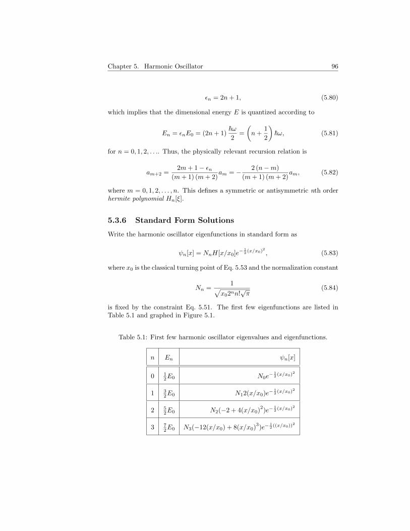
Chapter 5. Harmonic Oscillator 96
εn = 2n+ 1, (5.80)
which implies that the dimensional energy E is quantized according to
En = εnE0 = (2n+ 1)~ω2
=
(n+
1
2
)~ω, (5.81)
for n = 0, 1, 2, . . .. Thus, the physically relevant recursion relation is
am+2 =2m+ 1− εn
(m+ 1) (m+ 2)am = − 2 (n−m)
(m+ 1) (m+ 2)am, (5.82)
where m = 0, 1, 2, . . . , n. This defines a symmetric or antisymmetric nth orderhermite polynomial Hn[ξ].
5.3.6 Standard Form Solutions
Write the harmonic oscillator eigenfunctions in standard form as
ψn[x] = NnH[x/x0]e−12 (x/x0)
2
, (5.83)
where x0 is the classical turning point of Eq. 5.53 and the normalization constant
Nn =1√
x02nn!√π
(5.84)
is fixed by the constraint Eq. 5.51. The first few eigenfunctions are listed inTable 5.1 and graphed in Figure 5.1.
Table 5.1: First few harmonic oscillator eigenvalues and eigenfunctions.
n En ψn[x]
0 12E0 N0e
− 12 (x/x0)
2
1 32E0 N12(x/x0)e−
12 (x/x0)
2
2 52E0 N2(−2 + 4(x/x0)
2)e−
12 (x/x0)
2
3 72E0 N3(−12(x/x0) + 8(x/x0)
3)e−
12 ((x/x0))
2
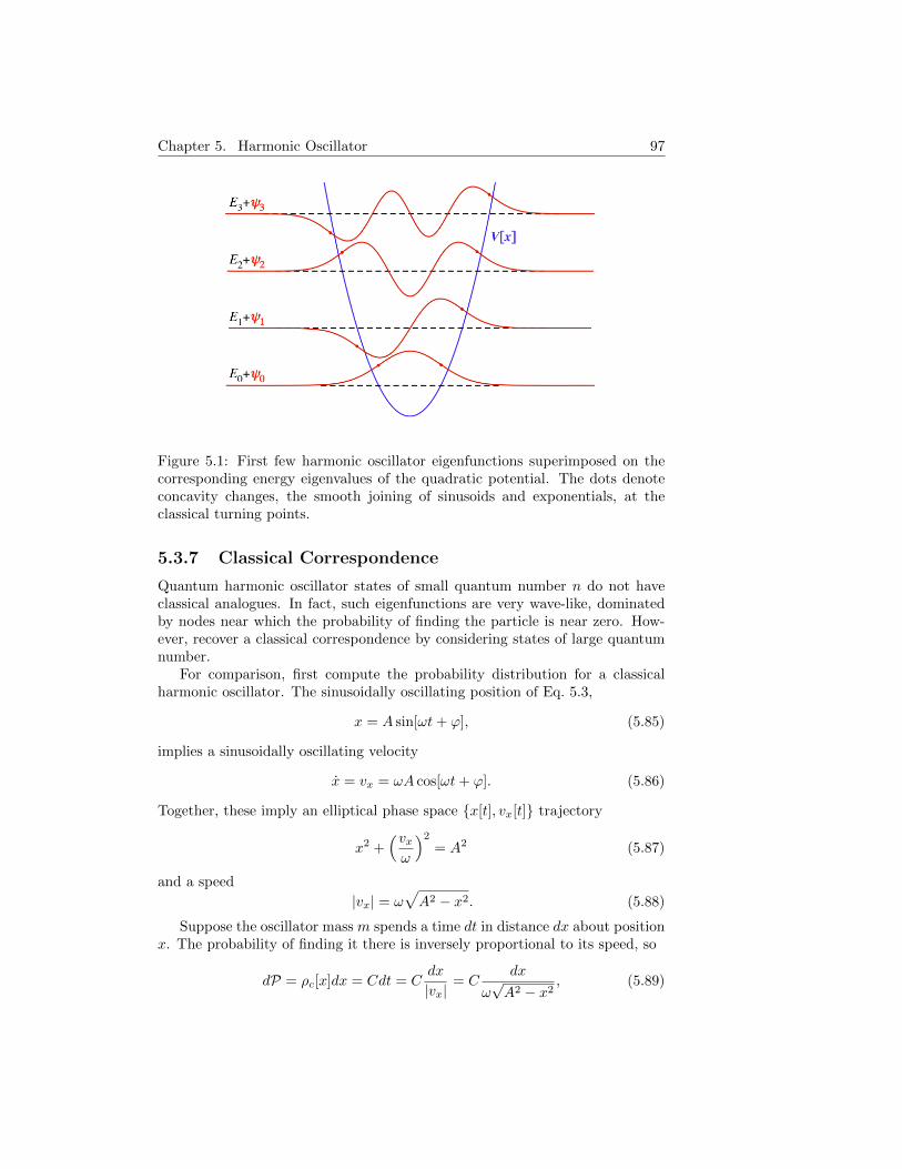
Chapter 5. Harmonic Oscillator 97
Figure 5.1: First few harmonic oscillator eigenfunctions superimposed on thecorresponding energy eigenvalues of the quadratic potential. The dots denoteconcavity changes, the smooth joining of sinusoids and exponentials, at theclassical turning points.
5.3.7 Classical Correspondence
Quantum harmonic oscillator states of small quantum number n do not haveclassical analogues. In fact, such eigenfunctions are very wave-like, dominatedby nodes near which the probability of finding the particle is near zero. How-ever, recover a classical correspondence by considering states of large quantumnumber.
For comparison, first compute the probability distribution for a classicalharmonic oscillator. The sinusoidally oscillating position of Eq. 5.3,
x = A sin[ωt+ ϕ], (5.85)
implies a sinusoidally oscillating velocity
x = vx = ωA cos[ωt+ ϕ]. (5.86)
Together, these imply an elliptical phase space {x[t], vx[t]} trajectory
x2 +(vxω
)2= A2 (5.87)
and a speed
|vx| = ω√A2 − x2. (5.88)
Suppose the oscillator mass m spends a time dt in distance dx about positionx. The probability of finding it there is inversely proportional to its speed, so
dP = ρc[x]dx = Cdt = Cdx
|vx|= C
dx
ω√A2 − x2
, (5.89)

Chapter 5. Harmonic Oscillator 98
Figure 5.2: At even the modest quantum number n = 20, the quantum proba-bility density corresponds well to the classical probability density.
where the normalization constant C is determined by the constraint
1 =
∫ A
−Aρc[x]dx =
∫ t0+T/2
t0
Cdt = CT
2. (5.90)
Thus, C = 2/T = ω/π, and the classical probability density is
ρc[x] =1
π√A2 − x2
. (5.91)
The classical turning point coordinate xn corresponding to the energy En isdefined by
(2n+ 1)E0 = En = V [xn] = E0
(xnx0
)2
, (5.92)
or
xn = x0√
2n+ 1. (5.93)
The quantum probability density follows the classical probability density withA = xn, as in Figure 5.2, for n = 20.
5.4 Angular Momentum
Harmonic oscillators in higher dimensions can have nonzero angular momentum.To model such oscillators, first study the eigenstates and eigenvalues of theangular momentum operators Ja = J†a, which are completely determined by theTable 4.3 commutation relations
[Ja, Jb] = i~ εabcJc. (5.94)
Chapter 5. Harmonic Oscillator 99
Although the components of angular momenta don’t commute with each other,they do commute with the the total angular momentum squared,
[J2, Jb] = [JaJa, Jb]
= Ja[Ja, Jb] + [Ja, Jb]Ja
= JaεabcJc + εabcJcJa
= εabcJaJc + εcbaJaJc
= (εabc + εcba)JaJc
= (εabc − εabc)JaJc= 0, (5.95)
and therefore share common eigenstates
J2|s, c〉 = ~2s|s, c〉, (5.96a)
Jz|s, c〉 = ~ c|s, c〉, (5.96b)
where the index choice a = 3 = z is conventional (from its special role incylindrical and spherical coordinates), and the factors of ~ make the squaredand component quantum numbers s and c dimensionless.
The expectation of any component squared⟨J2a
⟩=⟨s, c∣∣J2a
∣∣s, c⟩ =(⟨s, c∣∣J†a)(Ja
∣∣s, c⟩) = 〈ϕ|ϕ〉 ≥ 0 (5.97)
must be positive, and so the expectation of the total momentum squared⟨s, c∣∣J2∣∣s, c⟩ =
⟨s, c∣∣J2x |s, c
⟩+⟨s, c∣∣J2y
∣∣s, c⟩+⟨s, c∣∣J2z
∣∣s, c⟩ (5.98)
implies~2s =
⟨J2x
⟩+⟨J2y
⟩+ ~2c2 ≥ ~2c2 (5.99)
and−√s ≤ c ≤ +
√s. (5.100)
As with the harmonic oscillator, define the raising and lowering operators
J± = Jx ± iJy, (5.101)
which satisfy
[Jz, J±] = [Jz, Jx ± iJy] = [Jz, Jx]± i[Jz, Jy] = i~Jy ± ~Jx = ±~J± (5.102)
and
[J+, J−] = [Jx + iJy, Jx − iJy] = [Jx, Jx]− i[Jx, Jy] + i[Jy, Jx] + [Jy, Jy] = 2~Jz.(5.103)
First raise an eigenstate to J+|s, c〉 and measure Jz by applying the compo-nent operator to get
JzJ+|s, c〉 = (J+Jz + [Jz, J+])|s, c〉 = (J+Jz + ~J+)|s, c〉 = ~(c+ 1)J+|s, c〉(5.104)
Chapter 5. Harmonic Oscillator 100
and show thatJ+|s, c〉 ∝ |s, c+ 1〉 (5.105)
is an eigenstate of Jz with eigenvalue ~(c + 1). The raising operator mustannihilate the state with the maximum component
J+|s, cmax〉 = 0 (5.106)
or it would create an eigenstate with eigenvalue larger than the maximum. Since
J−J+ = (Jx−iJy)(Jx+iJy) = J2x+J2
y+i(JxJy−JyJx) = J2−J2z−~Jz, (5.107)
multiply Eq. 5.106 by the lowering operator to find
0 = J−J+|s, cmax〉 = ~2(s− c2max − cmax)|s, cmax〉 (5.108)
sos = cmax(cmax + 1). (5.109)
Next lower an eigenstate to J−|s, c〉 and measure Jz by applying the com-ponent operator to get
JzJ−|s, c〉 = (J−Jz + [Jz, J−])|s, c〉 = (J−Jz − ~J−)|s, c〉 = ~(c− 1)J−|s, c〉(5.110)
and show thatJ−|s, c〉 ∝ |s, c− 1〉 (5.111)
is an eigenstate of Jz with eigenvalue ~(c − 1). The lower operator must anni-hilate the state with the minimum component
J−|s, cmin〉 = 0 (5.112)
or it would create an eigenstate with eigenvalue smaller than the minimum.Since
J+J− = (Jx+iJy)(Jx−iJy) = J2x+J2
y−i(JxJy−JyJx) = J2−J2z +~Jz, (5.113)
multiply Eq. 5.112 by the raising operator to find
0 = J+J−|s, cmin〉 = ~2(s− c2min + cmin)|s, cmin〉 (5.114)
sos = −cmin(−cmin + 1). (5.115)
Equations 5.109 & 5.115 imply cmax = −cmin ≡ j so that s = j(j+ 1). Sincethe component quantum numbers c differ by integers, cmax − cmin = 2j is aninteger, and j is a “half integer”. Conventionally label the common eigenstatesof J2 and Jz by quantum numbers j and m = c so that
J2|j,m〉 = ~2j(j + 1)|j,m〉, (5.116a)
Jz|j,m〉 = ~ m|j,m〉, (5.116b)
where each angular momentum squared quantum number j = 0, 1/2, 1, 3/2, 2, . . .corresponds to 2j+1 values of angular momentum component quantum numberm = −j,−j + 1, . . . , j − 1, j, as in Fig. 5.3. In nature, fermions (like electrons)realize the half integer spin angular momentum and bosons (like photons) realizethe integer spin angular momentum.

Chapter 5. Harmonic Oscillator 101
Figure 5.3: Angular momentum quantum numbers for fermions (red dots) andbosons (black dots).
5.5 Two-Dimensional Harmonic Oscillator
5.5.1 Classical Case
An isotropic harmonic oscillator in the two-dimensional xy-plane has energy
E =1
2mp2x +
1
2mp2x +
mω2
2(x2 + y2), (5.117)
and angular momentum
~L = ~r × ~p = z(xpy − ypx). (5.118)
5.5.2 Eigenstates of Energy
Quantum mechanically, the Eq. 5.117 harmonic oscillator oscillator implies theHamiltonian operator
H =1
2mP 2x +
1
2mP 2y +
mω2
2(X2 + Y 2), (5.119)
where the energy spectrum of H follows algebraically from the Table 4.3 com-mutation relations
[X,Px] = i~, (5.120a)
[Y, Py] = i~, (5.120b)
with all others vanishing, and the hermeticity of the position and momentumoperators.

Chapter 5. Harmonic Oscillator 102
Mirroring the solution of the one-dimensional oscillator, introduce the di-mensionless position and momentum operators
x =X
x0=
√mω
~X, (5.121a)
y =Y
x0=
√mω
~Y, (5.121b)
px =Pxp0
=
√1
m~ωPx, (5.121c)
py =Pyp0
=
√1
m~ωPy, (5.121d)
and the annihilation or creation operators
ax =x+ ipx√
2, (5.122a)
ay =y + ipy√
2, (5.122b)
a†x =x− ipx√
2, (5.122c)
a†y =y − ipy√
2, (5.122d)
such that
x =ax + a†x√
2, (5.123a)
y =ay + a†y√
2, (5.123b)
px =ax − a†xi√
2, (5.123c)
py =ay − a†yi√
2, (5.123d)
and[ax, a
†x] = 1 = [ay, a
†y], (5.124)
with all others vanishing. The Hamiltonian “factorizes” into
H = ~ω(a†xax +
1
2
)+ ~ω
(a†yay +
1
2
)= ~ω
(Nx +
1
2
)+ ~ω
(Ny +
1
2
),
= ~ω (Nx +Ny + 1) . (5.125)
Chapter 5. Harmonic Oscillator 103
Since [Nx, Ny] = 0, there are simultaneous eigenstates |nx, ny〉 that can belowered
ax|nx, ny〉 =√nx|nx − 1, ny〉, (5.126a)
ay|nx, ny〉 =√ny|nx, ny − 1〉, (5.126b)
and raised
a†x|nx, ny〉 =√nx + 1|nx + 1, ny〉, (5.127a)
a†y|nx, ny〉 =√ny + 1|nx, ny + 1〉. (5.127b)
The orthonormal eigenstates of the number operators satisfy
Nx|nx, ny〉 = nx|nx, ny〉, (5.128a)
Ny|nx, ny〉 = ny|nx, ny〉, (5.128b)
and the orthonormal eigenstates of the Hamiltonian operator satisfy
H|nx, ny〉 = (nx + ny + 1)~ω|nx, ny〉, (5.129)
orH|E~n〉 = E~n|E~n〉, (5.130)
whereE~n = (n+ 1)~ω, (5.131)
and n = nx + ny. Because the eigenstates |3, 2〉 and |2, 3〉 correspond to thesame energy of 6~ω, the states are two-fold degenerate.
5.5.3 Eigenstates of Energy & Angular Momentum
Using Eqs. 5.121 & 5.123, the angular momentum operator
Lz = XPy − Y Px = i~(axa†y − a†xay) = L†z, (5.132)
as in Problem 5. Adding the relations
[axa†y − a†xay, a†xax] = +axa
†y + a†xay, (5.133a)
[axa†y − a†xay, a†yay] = −axa†y − a†xay, (5.133b)
implies[Lz, H] = 0, (5.134)
as in Problem 6, so the angular momentum and Hamiltonian operators will havecommon eigenstates. Obtain these by defining new raising and lower operators
a+ =ax + iay√
2, (5.135a)
a− =ax − iay√
2, (5.135b)
Chapter 5. Harmonic Oscillator 104
such that
ax =a+ + a−√
2, (5.136a)
ay =a+ − a−i√
2, (5.136b)
and
[a+, a†+] = 1 = [a−, a
†−], (5.137)
with all others vanishing.
The Hamiltonian operator
H
~ω= a†xax + a†yay + 1
=(a†+ + a†−)(a+ + a−)
2+
(a†+ − a†−)(a+ − a−)
2+ 1
= a†+a+ + a†−a− + 1
= N+ +N− + 1, (5.138)
and the angular momentum operator
Lz~
= iaxa†y − ia†xay
= ia†yax − ia†xay
= −(a†+ − a
†−)(a+ + a−)
2−
(a†+ + a†−)(a− − a−)
2
= −a†+a+ + a†−a−
= N− −N+. (5.139)
The lowering operators satisfy
a+|n+, n−〉 =√n+|n+ − 1, n−〉, (5.140a)
a−|n+, n−〉 =√n−|n+, n− − 1〉, (5.140b)
and the raising operators satisfy
a†+|n+, n−〉 =√n+ + 1|n+ + 1, n−〉, (5.141a)
a†−|n+, n−〉 =√n− + 1|n+, n− + 1〉, (5.141b)
The orthonormal eigenstates of the number operators satisfy
N+|n+, n−〉 = n+|n+, n−〉, (5.142a)
N−|n+, n−〉 = n−|n+, n−〉, (5.142b)
Chapter 5. Harmonic Oscillator 105
and the orthonormal eigenstates of the Hamiltonian and angular momentumoperators satisfy
H|n+, n−〉 = (n+ + n− + 1) ~ω |n+, n−〉, (5.143a)
Lz|n+, n−〉 = (n− − n+) ~ |n+, n−〉. (5.143b)
In terms of the sum and difference quantum numbers
n = n+ + n−, (5.144a)
m = n− − n+, (5.144b)
the dynamic operators are
H|n,m〉 = (n+ 1) ~ω |n,m〉, (5.145a)
Lz|n,m〉 = m ~ |n,m〉, (5.145b)
where n = 0, 1, 2, . . . and m = −n,−n + 2, . . . , n − 2, n. Thus for each energy,there are n + 1 angular momentum states, with equal numbers of positive andnegative momenta.
Chapter 5. Harmonic Oscillator 106
Problems
1. Justify the Eq. 5.36 creation operator normalization.
2. Sketch the five top-left rows and columns of the infinite square matrix rep-resentations for the annihilation a, creation a†, and number N operators.
3. Find the constant N0 in the Eq. 5.46 ground state wave function by en-forcing Eq. 5.51 normalization.
4. Generalize the technique of Section 5.2.5 to find the harmonic oscillatorfirst excited state position wave function ψ1[x] = 〈x|1〉.
5. Derive the Eq. 5.132 angular momentum operator expression, and showthat it is hermitian.
6. Derive the Eq. 5.133 identities and use them to show that the isotropicoscillator’s Hamiltonian and angular momentum operators commute.
Chapter 6
Hydrogen Atom
The hydrogen atom is the exactly solvable model that unlocked the quantumworld and underlies chemistry.
6.1 Classical Kepler Problem
The hydrogen atom problem is the quantum Kepler problem. The classicalKepler problem consist of a reduced mass article bound to an inverse distancepotential
V [r] = −κr, (6.1)
where κ = GMm and 1/µ = 1/m + 1/M . Associated with the 3 degrees offreedom of the particle are 2 ∗ 3 − 1 = 5 constants of the motion (and a 6threlated to the arbitrary origin of time). They are the total energy
E =p2
2µ− κ
r, (6.2)
the angular momentum~L = ~r × ~p, (6.3)
and the eccentricity (or Laplace-Runge-Lenz vector)
~e = r +~L× ~pµκ
, (6.4)
subject to the constraints~e · ~L = 0 (6.5)
and
e2 = 1 +2EL2
µκ2, (6.6)
giving 1 + 3 + 3 − 1 − 1 = 5 constants of the motion. The last constant of themotion, the eccentricity vector ~e, ensures that all bound orbits are closed, which
107
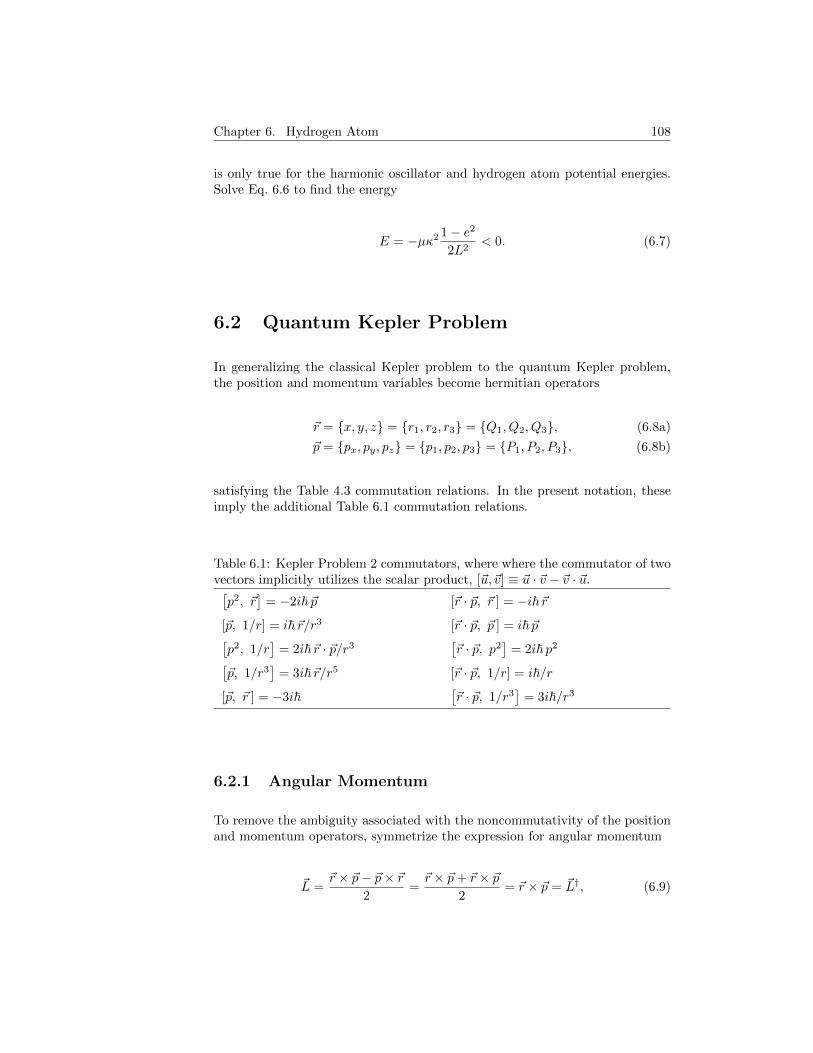
Chapter 6. Hydrogen Atom 108
is only true for the harmonic oscillator and hydrogen atom potential energies.Solve Eq. 6.6 to find the energy
E = −µκ2 1− e2
2L2< 0. (6.7)
6.2 Quantum Kepler Problem
In generalizing the classical Kepler problem to the quantum Kepler problem,the position and momentum variables become hermitian operators
~r = {x, y, z} = {r1, r2, r3} = {Q1, Q2, Q3}, (6.8a)
~p = {px, py, pz} = {p1, p2, p3} = {P1, P2, P3}, (6.8b)
satisfying the Table 4.3 commutation relations. In the present notation, theseimply the additional Table 6.1 commutation relations.
Table 6.1: Kepler Problem 2 commutators, where where the commutator of twovectors implicitly utilizes the scalar product, [~u,~v] ≡ ~u · ~v − ~v · ~u.[p2, ~r
]= −2i~ ~p [~r · ~p, ~r ] = −i~~r
[~p, 1/r] = i~~r/r3 [~r · ~p, ~p ] = i~ ~p[p2, 1/r
]= 2i~~r · ~p/r3
[~r · ~p, p2
]= 2i~ p2[
~p, 1/r3]
= 3i~~r/r5 [~r · ~p, 1/r] = i~/r
[~p, ~r ] = −3i~[~r · ~p, 1/r3
]= 3i~/r3
6.2.1 Angular Momentum
To remove the ambiguity associated with the noncommutativity of the positionand momentum operators, symmetrize the expression for angular momentum
~L =~r × ~p− ~p× ~r
2=~r × ~p+ ~r × ~p
2= ~r × ~p = ~L†, (6.9)
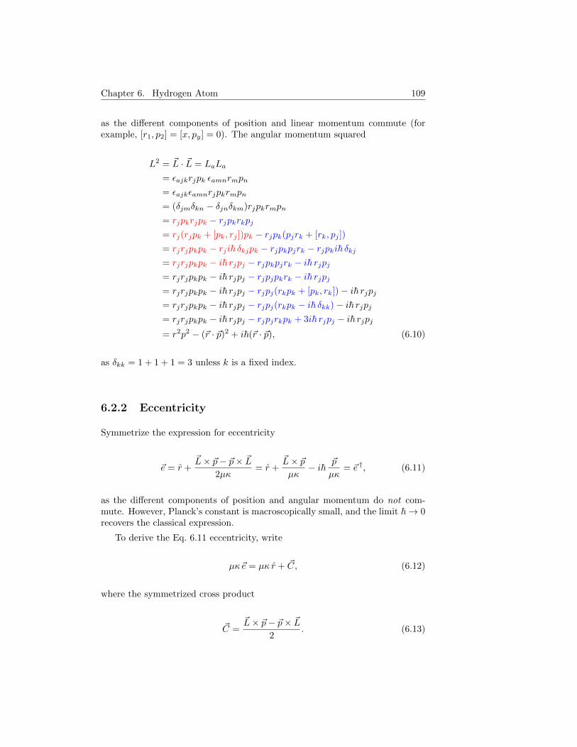
Chapter 6. Hydrogen Atom 109
as the different components of position and linear momentum commute (forexample, [r1, p2] = [x, py] = 0). The angular momentum squared
L2 = ~L · ~L = LaLa
= εajkrjpk εamnrmpn
= εajkεamnrjpkrmpn
= (δjmδkn − δjnδkm)rjpkrmpn
= rjpkrjpk − rjpkrkpj= rj(rjpk + [pk, rj ])pk − rjpk(pjrk + [rk, pj ])
= rjrjpkpk − rji~ δkjpk − rjpkpjrk − rjpki~ δkj= rjrjpkpk − i~ rjpj − rjpkpjrk − i~ rjpj= rjrjpkpk − i~ rjpj − rjpjpkrk − i~ rjpj= rjrjpkpk − i~ rjpj − rjpj(rkpk + [pk, rk])− i~ rjpj= rjrjpkpk − i~ rjpj − rjpj(rkpk − i~ δkk)− i~ rjpj= rjrjpkpk − i~ rjpj − rjpjrkpk + 3i~ rjpj − i~ rjpj= r2p2 − (~r · ~p)2 + i~(~r · ~p), (6.10)
as δkk = 1 + 1 + 1 = 3 unless k is a fixed index.
6.2.2 Eccentricity
Symmetrize the expression for eccentricity
~e = r +~L× ~p− ~p× ~L
2µκ= r +
~L× ~pµκ
− i~ ~p
µκ= ~e †, (6.11)
as the different components of position and angular momentum do not com-mute. However, Planck’s constant is macroscopically small, and the limit ~→ 0recovers the classical expression.
To derive the Eq. 6.11 eccentricity, write
µκ~e = µκ r + ~C, (6.12)
where the symmetrized cross product
~C =~L× ~p− ~p× ~L
2. (6.13)

Chapter 6. Hydrogen Atom 110
In components
2Ca = εajkLjpk − εajkpjLk= εajkεjmnrmpnpk − εajkpjεkmnrmpn= −εajkεkmn(rmpnpj + pjrmpn)
= −(δamδjn − δanδjm)(rmpnpj + pjrmpn)
= −rapjpj + rjpapj − pjrapj + pjrjpa
= −rapjpj + rjpapj − (rapj − i~ δja)pj + (rjpj − i~ δjj)pa= −rapjpj + rjpapj − rapjpj + i~ pa + rjpjpa − 3i~ pa= −2rapjpj + 2rjpjpa − 2i~ pa, (6.14)
so two forms of the cross product are
~C = −~r p2 + (~r · ~p)~p− i~ ~p = (~r × ~p)× ~p− i~ ~p = ~L× ~p− i~ ~p, (6.15a)
~C = −~r p2 + ~p(~r · ~p), (6.15b)
where the second form is courtesy of Table 6.1. Thus, two forms of the eccen-tricity are
µκ~e = µκ r + ~L× ~p− i~ ~p, (6.16a)
µκ~e = ~p(~r · ~p)− ~r(p2 − µκ
r
). (6.16b)
If φ = ~r · ~p and θ = p2 − µκ/r, then the eccentricity squared
(µκ e)2 = µκ~e · µκ~e= (~pφ− ~rθ) · (~pφ− ~rθ)
= ~pφ · ~pφ− ~pφ · ~r~θ − ~rθ · ~pφ+ ~rθ · ~rφ. (6.17)
The Table 6.1 commutators imply
~pφ · ~pφ = pnφ pnφ
= pn(pnφ+ i~ pn)φ
= pnpnφ2 + i~ pnpnφ
= p2φ2 + i~ p2 (6.18)
and similarly
−~pφ · ~r~θ = −p2φ2 − ~2p2 +µκ
rφ2 − 2i~
µκ
rφ (6.19)
and
−~rθ · ~pφ = −p2φ2 +µκ
rφ2 − 2i~ p2φ (6.20)
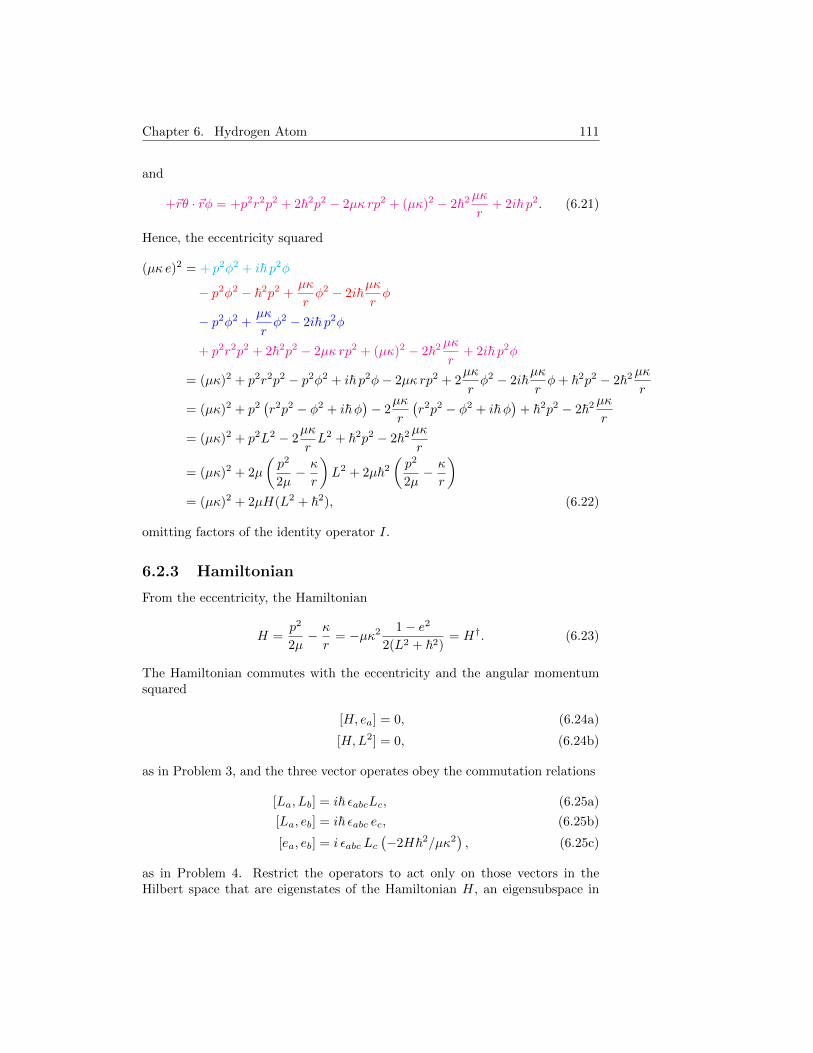
Chapter 6. Hydrogen Atom 111
and
+~rθ · ~rφ = +p2r2p2 + 2~2p2 − 2µκ rp2 + (µκ)2 − 2~2µκ
r+ 2i~ p2. (6.21)
Hence, the eccentricity squared
(µκ e)2 = + p2φ2 + i~ p2φ
− p2φ2 − ~2p2 +µκ
rφ2 − 2i~
µκ
rφ
− p2φ2 +µκ
rφ2 − 2i~ p2φ
+ p2r2p2 + 2~2p2 − 2µκ rp2 + (µκ)2 − 2~2µκ
r+ 2i~ p2φ
= (µκ)2 + p2r2p2 − p2φ2 + i~ p2φ− 2µκ rp2 + 2µκ
rφ2 − 2i~
µκ
rφ+ ~2p2 − 2~2
µκ
r
= (µκ)2 + p2(r2p2 − φ2 + i~φ
)− 2
µκ
r
(r2p2 − φ2 + i~φ
)+ ~2p2 − 2~2
µκ
r
= (µκ)2 + p2L2 − 2µκ
rL2 + ~2p2 − 2~2
µκ
r
= (µκ)2 + 2µ
(p2
2µ− κ
r
)L2 + 2µ~2
(p2
2µ− κ
r
)= (µκ)2 + 2µH(L2 + ~2), (6.22)
omitting factors of the identity operator I.
6.2.3 Hamiltonian
From the eccentricity, the Hamiltonian
H =p2
2µ− κ
r= −µκ2 1− e2
2(L2 + ~2)= H†. (6.23)
The Hamiltonian commutes with the eccentricity and the angular momentumsquared
[H, ea] = 0, (6.24a)
[H,L2] = 0, (6.24b)
as in Problem 3, and the three vector operates obey the commutation relations
[La, Lb] = i~ εabcLc, (6.25a)
[La, eb] = i~ εabc ec, (6.25b)
[ea, eb] = i εabc Lc(−2H~2/µκ2
), (6.25c)
as in Problem 4. Restrict the operators to act only on those vectors in theHilbert space that are eigenstates of the Hamiltonian H, an eigensubspace in
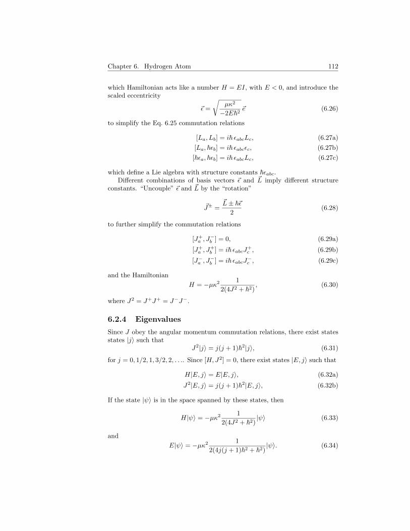
Chapter 6. Hydrogen Atom 112
which Hamiltonian acts like a number H = EI, with E < 0, and introduce thescaled eccentricity
~ε =
√µκ2
−2E~2~e (6.26)
to simplify the Eq. 6.25 commutation relations
[La, Lb] = i~ εabcLc, (6.27a)
[La, ~εb] = i~ εabcεc, (6.27b)
[~εa, ~εb] = i~ εabcLc, (6.27c)
which define a Lie algebra with structure constants ~εabc.Different combinations of basis vectors ~ε and ~L imply different structure
constants. “Uncouple” ~ε and ~L by the “rotation”
~J± =~L± ~~ε
2(6.28)
to further simplify the commutation relations
[J+a , J
−b ] = 0, (6.29a)
[J+a , J
+b ] = i~ εabcJ+
c , (6.29b)
[J−a , J−b ] = i~ εabcJ−c , (6.29c)
and the Hamiltonian
H = −µκ2 1
2(4J2 + ~2), (6.30)
where J2 = J+J+ = J−J−.
6.2.4 Eigenvalues
Since J obey the angular momentum commutation relations, there exist statesstates |j〉 such that
J2|j〉 = j(j + 1)~2|j〉, (6.31)
for j = 0, 1/2, 1, 3/2, 2, . . .. Since [H,J2] = 0, there exist states |E, j〉 such that
H|E, j〉 = E|E, j〉, (6.32a)
J2|E, j〉 = j(j + 1)~2|E, j〉, (6.32b)
If the state |ψ〉 is in the space spanned by these states, then
H|ψ〉 = −µκ2 1
2(4J2 + ~2)|ψ〉 (6.33)
and
E|ψ〉 = −µκ2 1
2(4j(j + 1)~2 + ~2)|ψ〉. (6.34)
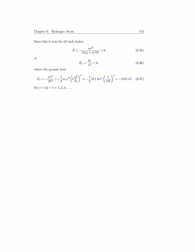
Chapter 6. Hydrogen Atom 113
Since this is true for all such states,
E = − µκ2
2(2j + 1)2~2< 0 (6.35)
or
En =E1
n2< 0, (6.36)
where the ground state
E1 = −µκ2
2~2= −1
2mec
2
(kq2e~c
)2
≈ −1
2511 keV
(1
137
)2
= −13.6 eV, (6.37)
for n = 2j + 1 = 1, 2, 3, . . ..
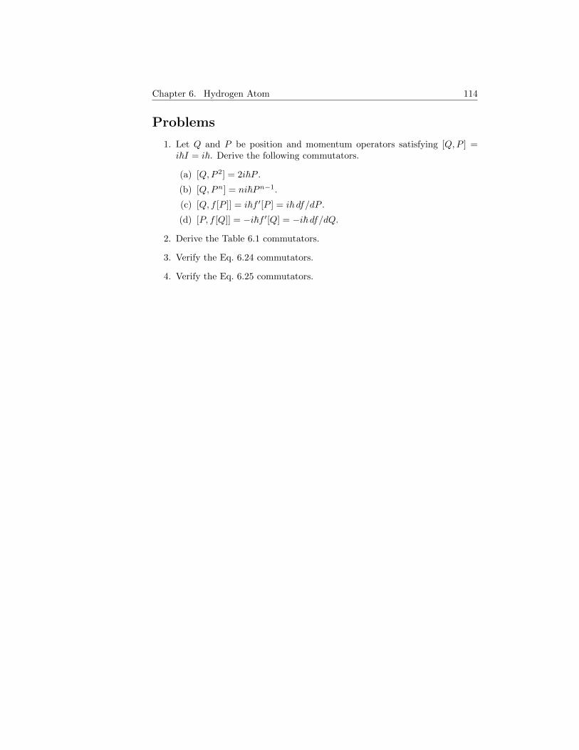
Chapter 6. Hydrogen Atom 114
Problems
1. Let Q and P be position and momentum operators satisfying [Q,P ] =i~I = i~. Derive the following commutators.
(a) [Q,P 2] = 2i~P .
(b) [Q,Pn] = ni~Pn−1.
(c) [Q, f [P ]] = i~f ′[P ] = i~ df/dP .
(d) [P, f [Q]] = −i~f ′[Q] = −i~ df/dQ.
2. Derive the Table 6.1 commutators.
3. Verify the Eq. 6.24 commutators.
4. Verify the Eq. 6.25 commutators.
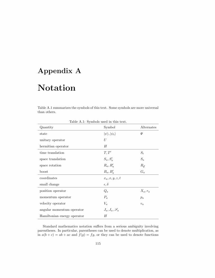
Appendix A
Notation
Table A.1 summarizes the symbols of this text. Some symbols are more universalthan others.
Table A.1: Symbols used in this text.
Quantity Symbol Alternates
state |ψ〉, |ψt〉 Ψ
unitary operator U
hermitian operator H
time translation T, T ′ St
space translation Sa, S′a Sa
space rotation Ra, R′a R~θ
boost Ba, B′a Ga
coordinates xa, x, y, z, t
small change ε, δ
position operator Qa Xa, ra
momentum operator Pa pa
velocity operator Va va
angular momentum operator Ja, Ja,Sa
Hamiltonian energy operator H
Standard mathematics notation suffers from a serious ambiguity involvingparentheses. In particular, parentheses can be used to denote multiplication, asin a(b + c) = ab + ac and f(g) = fg, or they can be used to denote functions
115

Appendix A. Notation 116
evaluated at arguments, as in f(t) and g(b+c). It can be a struggle to determinethe intended meaning from context.
To avoid ambiguity, this text always uses round parentheses (•) to groupfor multiplication and square brackets [•] to list function arguments. Thus,a(b) = ab denotes the product of two factors a and b, while f [x] denotes afunction f evaluated at an argument x. Mathematica [13] employs the sameconvention.
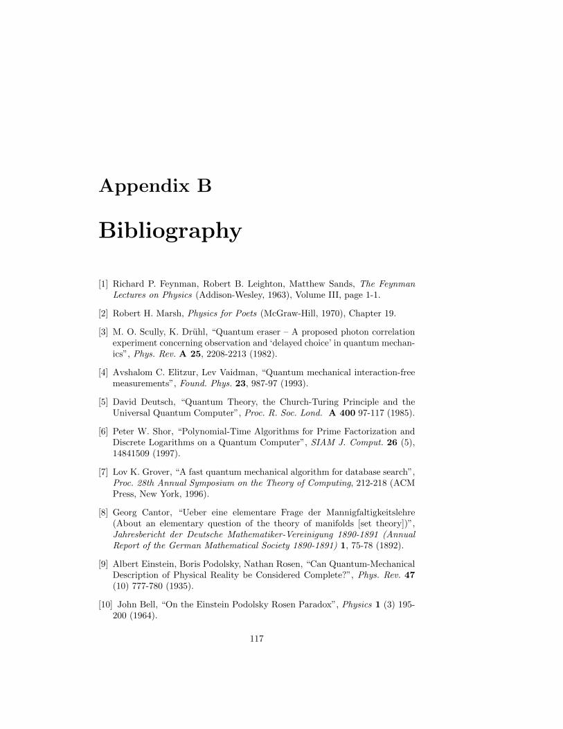
Appendix B
Bibliography
[1] Richard P. Feynman, Robert B. Leighton, Matthew Sands, The FeynmanLectures on Physics (Addison-Wesley, 1963), Volume III, page 1-1.
[2] Robert H. Marsh, Physics for Poets (McGraw-Hill, 1970), Chapter 19.
[3] M. O. Scully, K. Druhl, “Quantum eraser – A proposed photon correlationexperiment concerning observation and ‘delayed choice’ in quantum mechan-ics”, Phys. Rev. A 25, 2208-2213 (1982).
[4] Avshalom C. Elitzur, Lev Vaidman, “Quantum mechanical interaction-freemeasurements”, Found. Phys. 23, 987-97 (1993).
[5] David Deutsch, “Quantum Theory, the Church-Turing Principle and theUniversal Quantum Computer”, Proc. R. Soc. Lond. A 400 97-117 (1985).
[6] Peter W. Shor, “Polynomial-Time Algorithms for Prime Factorization andDiscrete Logarithms on a Quantum Computer”, SIAM J. Comput. 26 (5),14841509 (1997).
[7] Lov K. Grover, “A fast quantum mechanical algorithm for database search”,Proc. 28th Annual Symposium on the Theory of Computing, 212-218 (ACMPress, New York, 1996).
[8] Georg Cantor, “Ueber eine elementare Frage der Mannigfaltigkeitslehre(About an elementary question of the theory of manifolds [set theory])”,Jahresbericht der Deutsche Mathematiker-Vereinigung 1890-1891 (AnnualReport of the German Mathematical Society 1890-1891) 1, 75-78 (1892).
[9] Albert Einstein, Boris Podolsky, Nathan Rosen, “Can Quantum-MechanicalDescription of Physical Reality be Considered Complete?”, Phys. Rev. 47(10) 777-780 (1935).
[10] John Bell, “On the Einstein Podolsky Rosen Paradox”, Physics 1 (3) 195-200 (1964).
117

Appendix B. Bibliography 118
[11] Thomas F. Jordan, “Why −i∇ is the momentum”, Am. J. Phys. 43, 1089-1093 (1975).
[12] Leslie E. Ballentine, Quantum Mechanics (Prentice Hall, 1990).
[13] Wolfram Research, Inc., Mathematica, Version 9.0, Champaign, IL (2010).


![Quantum Mechanics relativistic quantum mechanics (RQM) · Quantum Mechanics_ relativistic quantum mechanics (RQM) ... [2] A postulate of quantum mechanics is that the time evolution](https://static.fdocuments.in/doc/165x107/5b6dfe707f8b9aed178e053e/quantum-mechanics-relativistic-quantum-mechanics-rqm-quantum-mechanics-relativistic.jpg)