Introduction to Quantum Computation - PHY 5650mucciolo/Aula1-4.pdfIntroduction to Quantum...
65
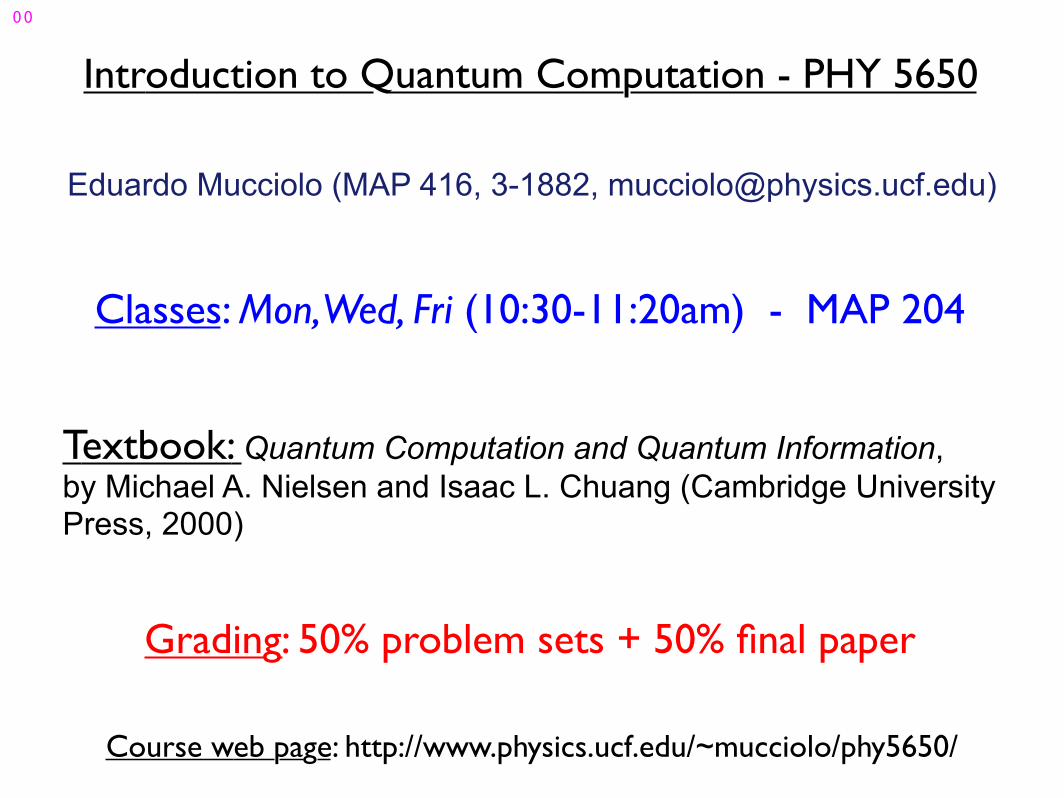
Intr oduction to Quantum Computation - PHY 5650 Classes: Mon,Wed, Fri (10:30-11:20am) - MAP 204 Eduardo Mucciolo (MAP 416, 3-1882, [email protected]) T extbook: Quantum Computation and Quantum Information, by Michael A. Nielsen and Isaac L. Chuang (Cambridge University Press, 2000) Grading: 50% problem sets + 50% final paper Course w eb page: http://www.physics.ucf.edu/~mucciolo/phy5650/ 00
Transcript of Introduction to Quantum Computation - PHY 5650mucciolo/Aula1-4.pdfIntroduction to Quantum...
Introduction to Quantum Computation - PHY 5650
Classes: Mon, Wed, Fri (10:30-11:20am) - MAP 204
Eduardo Mucciolo (MAP 416, 3-1882, [email protected])
Textbook: Quantum Computation and Quantum Information, by Michael A. Nielsen and Isaac L. Chuang (Cambridge University Press, 2000)
Grading: 50% problem sets + 50% final paper
Course web page: http://www.physics.ucf.edu/~mucciolo/phy5650/
00
CALENDAR −− SPRING 2005
(8)
10 (1) 12 (2)
26 (6) 28 (7)
21 (5)
14 (3)
10 (1) = Regular class day (#1)
= Problem set due
April
18
M
11
W F
01
06 (29)
13
25 (37)
20
15
22
(30)
(27)
(28)
27
04 08(31)
(34) (35)
(33)
(36)
29
(32)
January
Caption:
February
21
M W
02
F
04
07 (11) 09 (12)
28 (19)
23 (17)
21
25 (18)
11 (13)
(9) (10)
(15)
March
21
M
14
W
02
F
04
07 09 (23)
16
28 (25)
23
21
25
11 (24)
(20) (21)
(22)
(26)30
24
03
M
17
W
05
F
07
17 = Holiday
21 = Spring break 14 = No class
16 (14)14(16)
19 (4)
31
01
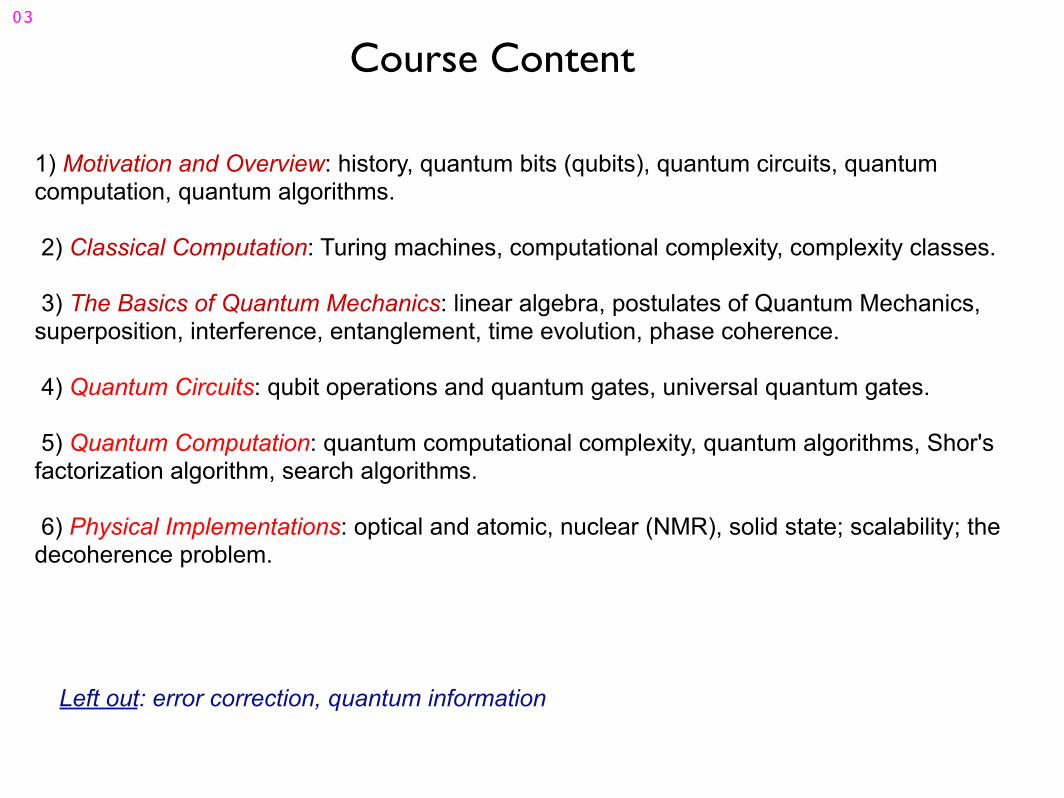
1) Motivation and Overview: history, quantum bits (qubits), quantum circuits, quantum computation, quantum algorithms.
2) Classical Computation: Turing machines, computational complexity, complexity classes.
3) The Basics of Quantum Mechanics: linear algebra, postulates of Quantum Mechanics, superposition, interference, entanglement, time evolution, phase coherence.
4) Quantum Circuits: qubit operations and quantum gates, universal quantum gates.
5) Quantum Computation: quantum computational complexity, quantum algorithms, Shor's factorization algorithm, search algorithms.
6) Physical Implementations: optical and atomic, nuclear (NMR), solid state; scalability; the decoherence problem.
Course Content
Left out: error correction, quantum information
03
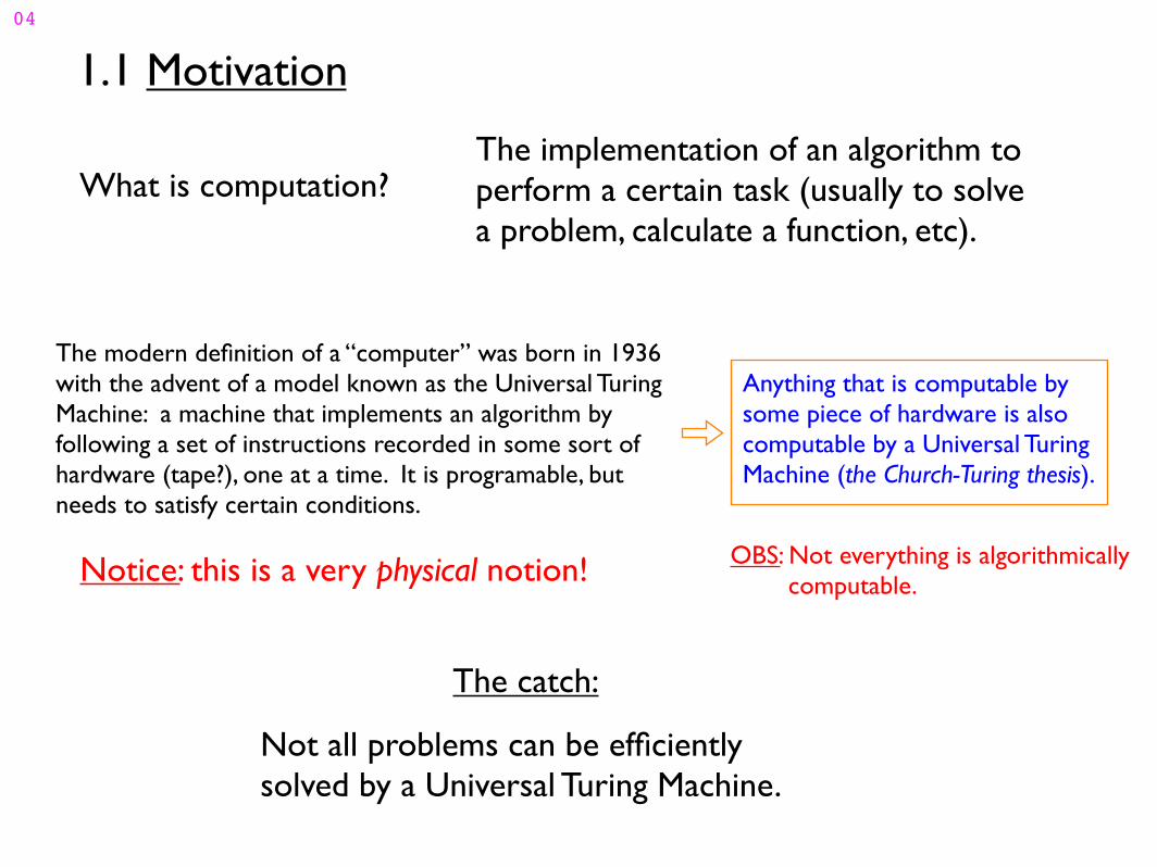
1.1 Motivation
What is computation?The implementation of an algorithm to perform a certain task (usually to solve a problem, calculate a function, etc).
The modern definition of a “computer” was born in 1936 with the advent of a model known as the Universal Turing Machine: a machine that implements an algorithm by following a set of instructions recorded in some sort of hardware (tape?), one at a time. It is programable, but needs to satisfy certain conditions.
Notice: this is a very physical notion!
The catch:
Not all problems can be efficientlysolved by a Universal Turing Machine.
OBS: Not everything is algorithmically computable.
Anything that is computable by some piece of hardware is also computable by a Universal Turing Machine (the Church-Turing thesis).
04
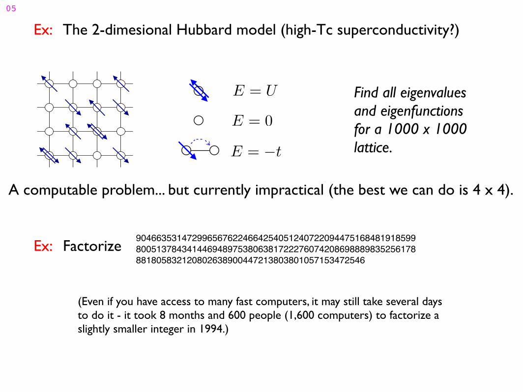
Ex: The 2-dimesional Hubbard model (high-Tc superconductivity?)
E = U
E = 0
E = −t
Find all eigenvaluesand eigenfunctions for a 1000 x 1000 lattice.
A computable problem... but currently impractical (the best we can do is 4 x 4).
Ex: Factorize90466353147299656762246642540512407220944751684819185998005137843414469489753806381722276074208698889835256178881805832120802638900447213803801057153472546
(Even if you have access to many fast computers, it may still take several days to do it - it took 8 months and 600 people (1,600 computers) to factorize a slightly smaller integer in 1994.)
05
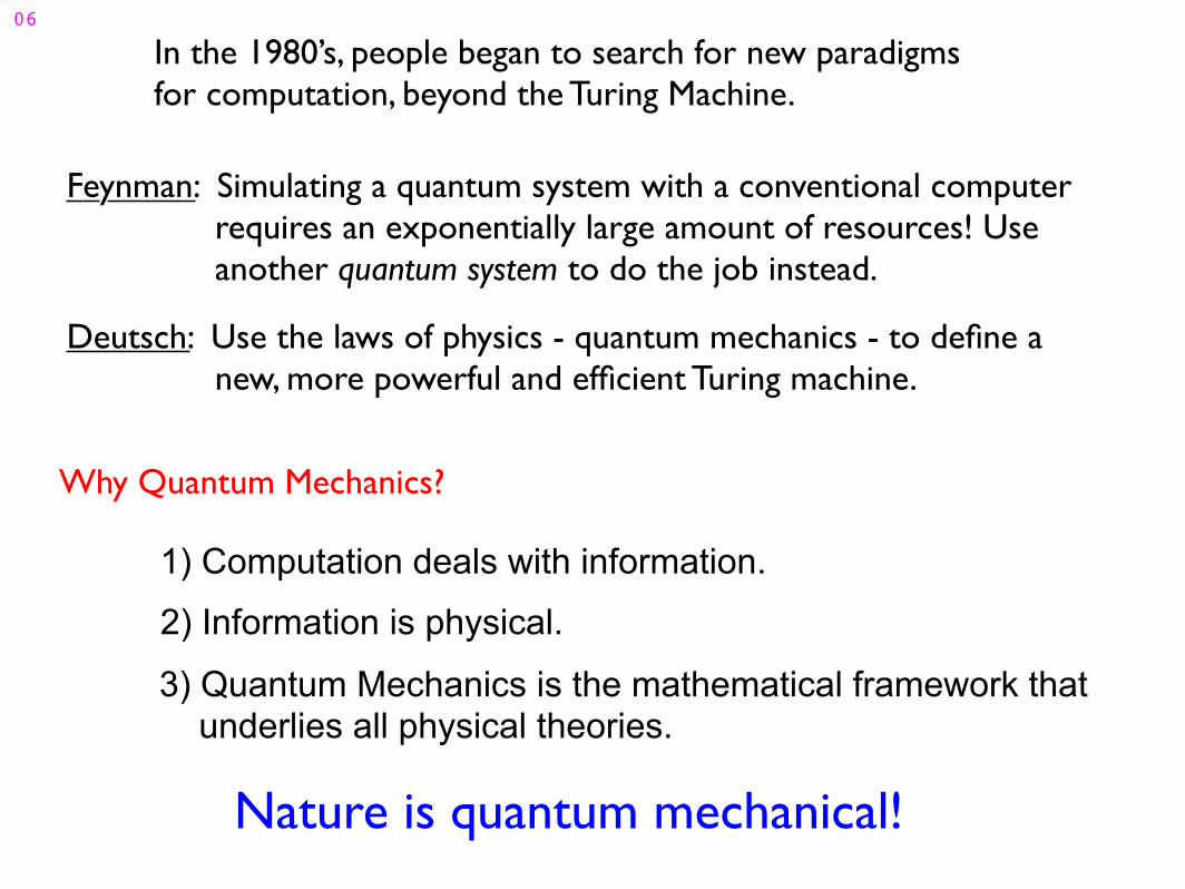
Nature is quantum mechanical!
In the 1980’s, people began to search for new paradigmsfor computation, beyond the Turing Machine.
Feynman: Simulating a quantum system with a conventional computer requires an exponentially large amount of resources! Use another quantum system to do the job instead.
Deutsch: Use the laws of physics - quantum mechanics - to define a new, more powerful and efficient Turing machine.
Why Quantum Mechanics?
1) Computation deals with information.
2) Information is physical.
3) Quantum Mechanics is the mathematical framework that underlies all physical theories.
06
The rules provide by Quantum Mechanicsdescribe physical phenomena at all length scales, from the behavior of elementary particles to the structure of the universe.
Conventional computers may be able to simulate classical problems (turbulence, diffusion, etc.) efficiently, but it will take a computer based on quantum mechanics to simulate a quantum system with tangible resources (time, memory, etc).
Quantum Computation began to take form in the mid 1980’s, but the “quantum leap” only happened in 1994, with the demonstration of a “killer application” by Shor: A quantum algorithm that factorizes any integer efficiently.
07
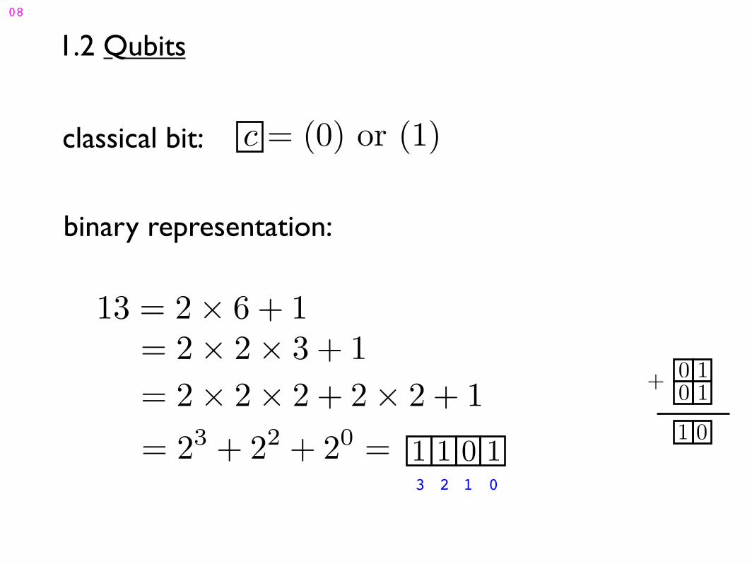
1.2 Qubits
classical bit: c = (0) or (1)
binary representation:
13 = 2 × 6 + 1
= 2 × 2 × 3 + 1
= 2 × 2 × 2 + 2 × 2 + 1
= 23
+ 22
+ 20
= 1 1 0 1
3 2 1 0
0 1
0 1
1 0
+
08
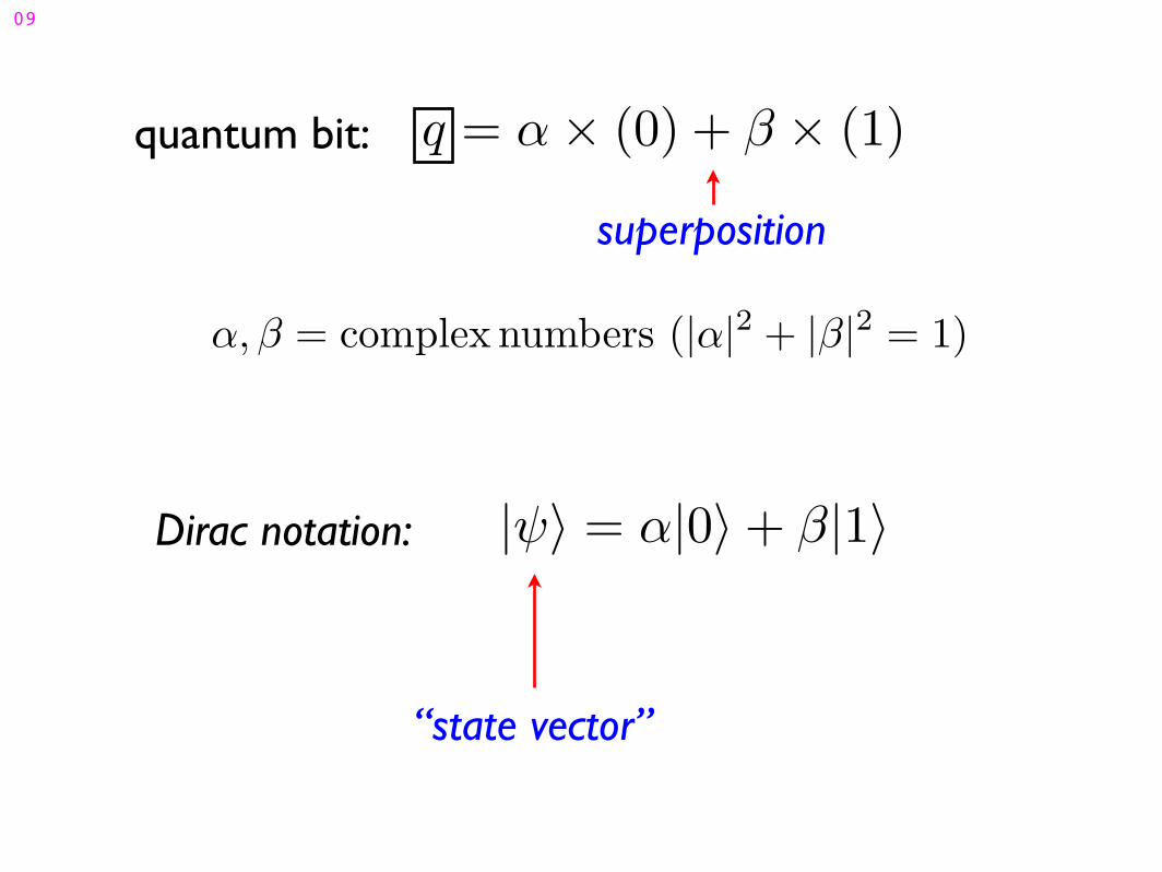
α, β = complex numbers (|α|2 + |β|2 = 1)
q = α × (0) + β × (1)quantum bit:
superposition
Dirac notation: |ψ〉 = α|0〉 + β|1〉
“state vector”
09
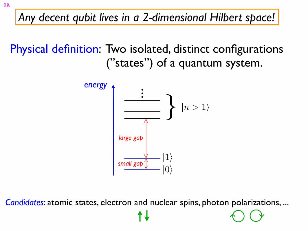
Any decent qubit lives in a 2-dimensional Hilbert space!
Physical definition: Two isolated, distinct configurations (”states”) of a quantum system.
|0〉
|1〉
}large gap
small gap
energy
|n > 1〉
Candidates: atomic states, electron and nuclear spins, photon polarizations, ...
0A
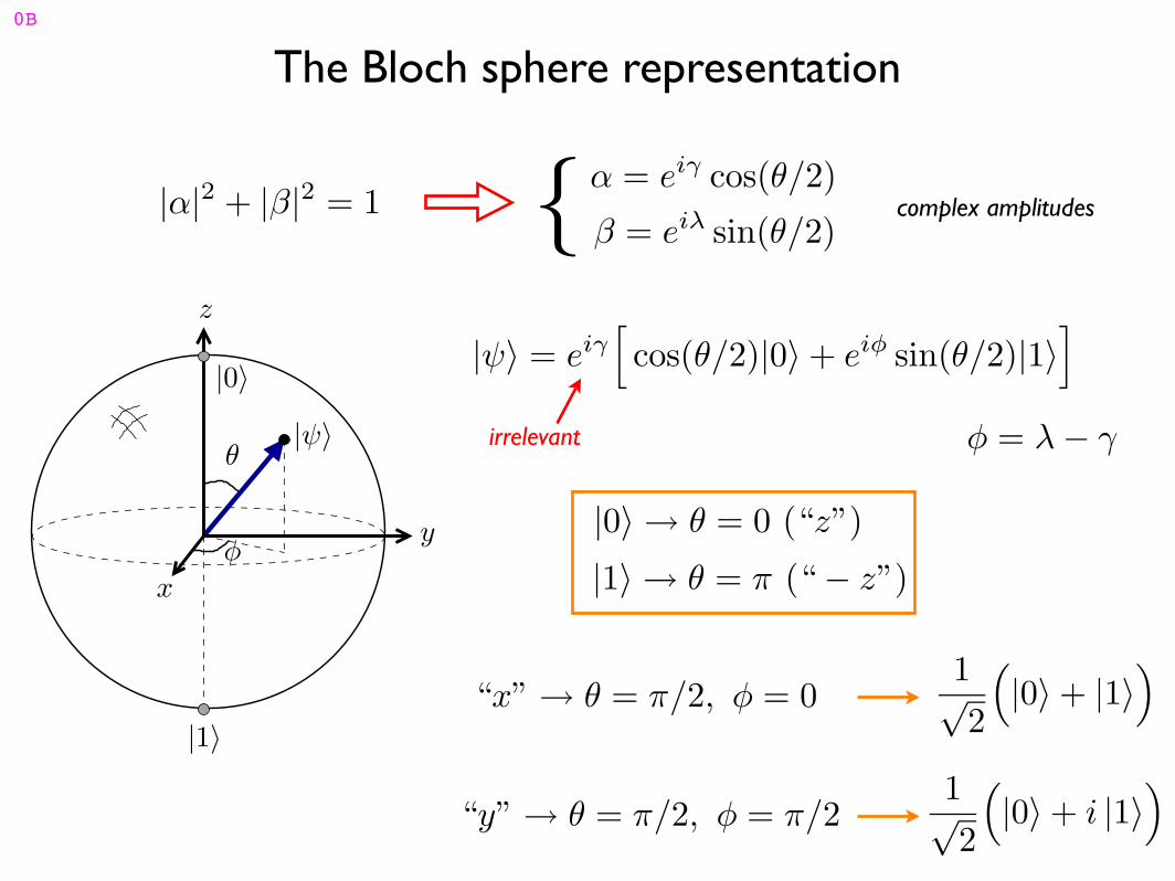
The Bloch sphere representation
|0〉 → θ = 0 (“z”)
|1〉 → θ = π (“ − z”)
|1〉
yφ
x
θ|ψ〉
|0〉
z
|ψ〉 = eiγ[cos(θ/2)|0〉 + eiφ sin(θ/2)|1〉
]
φ = λ − γirrelevant
“x” → θ = π/2, φ = 0
“y” → θ = π/2, φ = π/2
1√2
(|0〉 + |1〉
)
1√2
(|0〉 + i |1〉
)
|α|2 + |β|2 = 1 { complex amplitudesα = eiγ cos(θ/2)
β = eiλ sin(θ/2)
0B
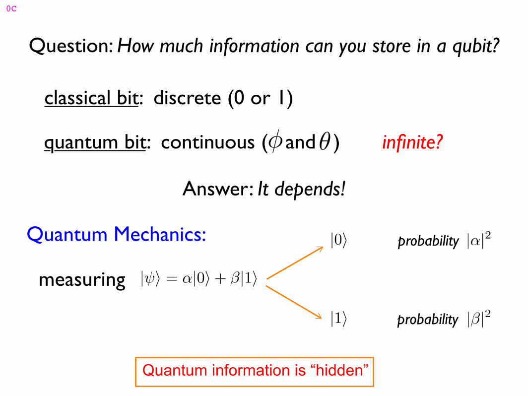
Question: How much information can you store in a qubit?
classical bit: discrete (0 or 1)
quantum bit: continuous ( and )φ θ infinite?
Answer: It depends!
|ψ〉 = α|0〉 + β|1〉
|α|2
|β|2
Quantum Mechanics:
measuring
|0〉
|1〉
probability
probability
Quantum information is “hidden”
0C
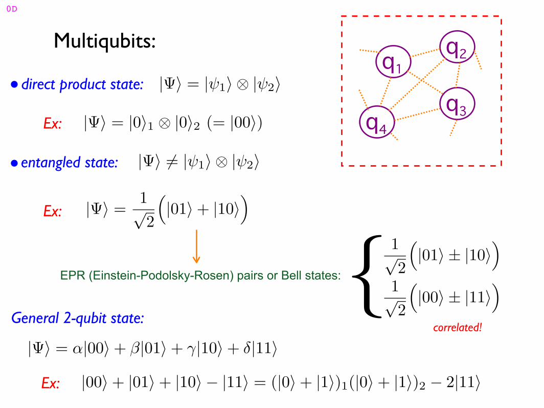
Multiqubits:q1
q2
q4
q3
|Ψ〉 "= |ψ1〉 ⊗ |ψ2〉
|Ψ〉 =1√2
(|01〉 + |10〉
)entangled state:
Ex:
|Ψ〉 = |ψ1〉 ⊗ |ψ2〉
|Ψ〉 = |0〉1 ⊗ |0〉2 (= |00〉)
direct product state:
Ex:
|Ψ〉 = α|00〉 + β|01〉 + γ|10〉 + δ|11〉
General 2-qubit state:
Ex: |00〉 + |01〉 + |10〉 − |11〉 = (|0〉 + |1〉)1(|0〉 + |1〉)2 − 2|11〉
EPR (Einstein-Podolsky-Rosen) pairs or Bell states:
1√2
(|01〉± |10〉
)
1√2
(|00〉± |11〉
){correlated!
0D
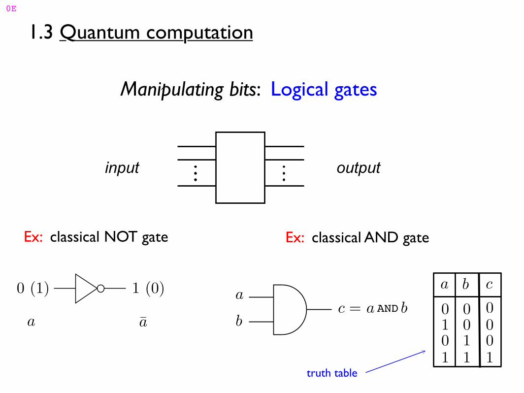
1.3 Quantum computation
Manipulating bits: Logical gates
input output
Ex: classical AND gate
a b
0
1
1
0
0
1
0
0
0 0
1 1
c
a
ba bANDc =
Ex: classical NOT gate
0 (1) 1 (0)
a a
truth table
0E
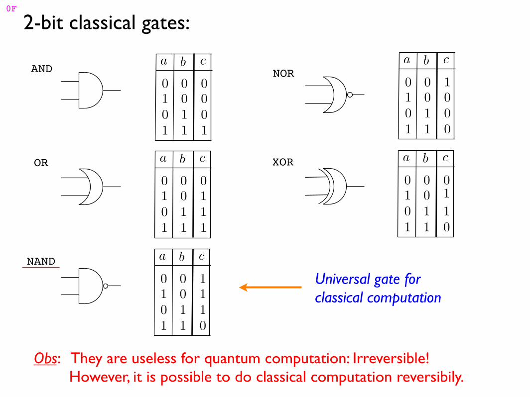
2-bit classical gates:
AND0
1
a b c
0
0
0
0
1
1
1 1
0
0
OR0
1
a b c
0
0
0
0
1
1
1 1
1
1
NAND0
1
a b c
0
0
0
1
1
1
1
0
1
1
NOR0
1
a b c
0
0
0
01
1
1
0
0
1
XOR
1
0
1
a b c
0
0
0
01
1
1
0
1
Universal gate for classical computation
Obs: They are useless for quantum computation: Irreversible! However, it is possible to do classical computation reversibily.
0F
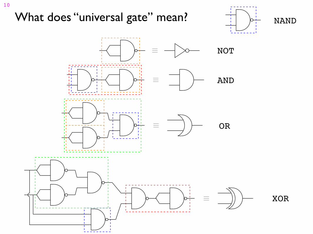
What does “universal gate” mean? NAND
NOT
AND
OR
XOR
10
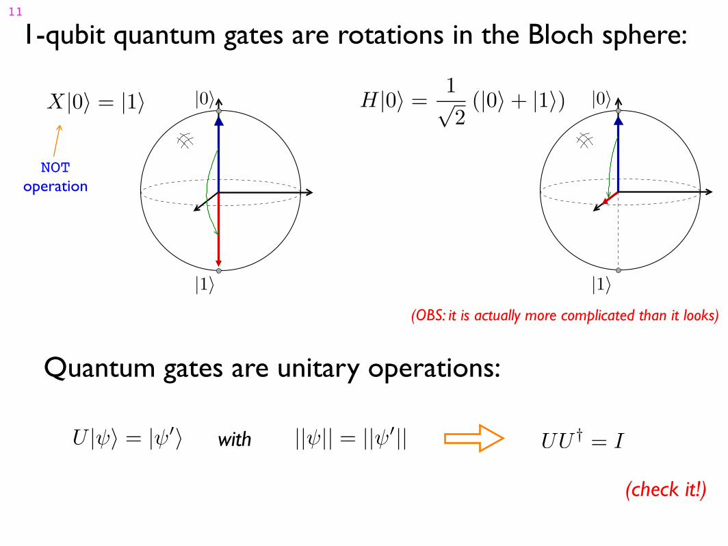
Quantum gates are unitary operations:
U |ψ〉 = |ψ′〉 ||ψ|| = ||ψ′|| UU†
= Iwith
(check it!)
1-qubit quantum gates are rotations in the Bloch sphere:
X|0〉 = |1〉
|1〉
|0〉 H|0〉 =1√2
(|0〉 + |1〉) |0〉
|1〉
(OBS: it is actually more complicated than it looks)
NOToperation
11
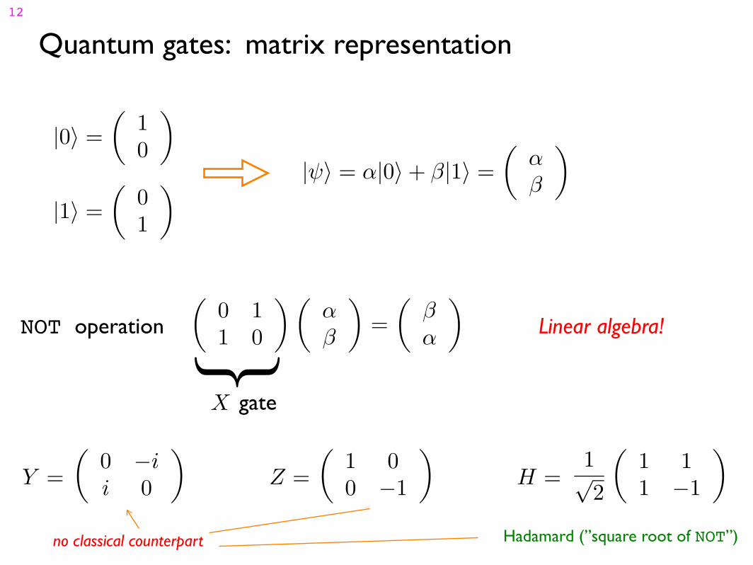
Quantum gates: matrix representation
|0〉 =
(1
0
)
|1〉 =
(0
1
) |ψ〉 = α|0〉 + β|1〉 =
(αβ
)
(1 0
0 −1
)(0 −i
i 0
)1√
2
(1 1
1 −1
)Y = H =Z =
Hadamard (”square root of NOT”)
(0 1
1 0
)(αβ
)=
(βα
)NOT operation
X
{
gate
Linear algebra!
no classical counterpart
12
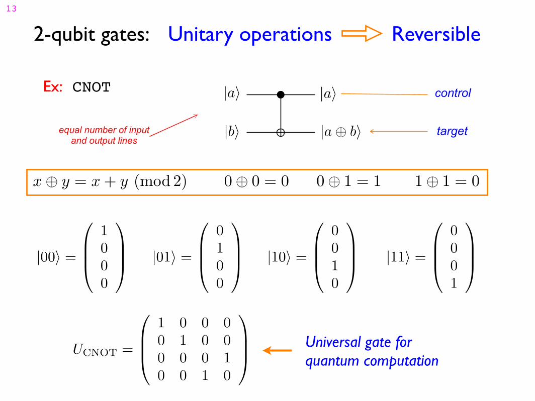
2-qubit gates: Unitary operations Reversible
Universal gate for quantum computation
UCNOT =
1 0 0 0
0 1 0 0
0 0 0 1
0 0 1 0
Ex: CNOT |a〉
|b〉
|a〉
|a ⊕ b〉
control
targetequal number of inputand output lines
0 ⊕ 0 = 0 0 ⊕ 1 = 1x ⊕ y = x + y (mod 2) 1 ⊕ 1 = 0
|00〉 =
1
0
0
0
|11〉 =
0
0
0
1
|01〉 =
0
1
0
0
|10〉 =
0
0
1
0
13
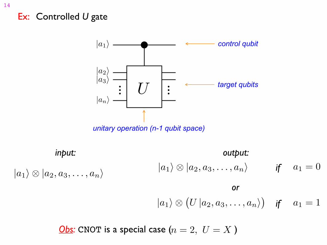
Ex: Controlled U gate
control qubit
target qubits
|a1〉
|a3〉
|an〉
|a2〉
U
unitary operation (n-1 qubit space)
|a1〉 ⊗ |a2, a3, . . . , an〉
|a1〉 ⊗(U |a2, a3, . . . , an〉
)
|a1〉 ⊗ |a2, a3, . . . , an〉 a1 = 0
a1 = 1
if
if
input: output:
or
Obs: CNOT is a special case ( )n = 2, U = X
14
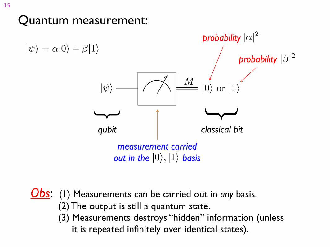
Quantum measurement:
|ψ〉 = α|0〉 + β|1〉
|ψ〉M
|0〉 or |1〉
} }qubit classical bit
|0〉, |1〉measurement carried
out in the basis
|α|2
|β|2
probability
probability
Obs: (1) Measurements can be carried out in any basis. (2) The output is still a quantum state. (3) Measurements destroys “hidden” information (unless it is repeated infinitely over identical states).
15
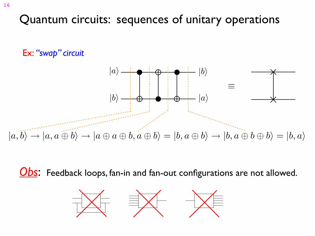
Quantum circuits: sequences of unitary operations
Ex: “swap” circuit
|a〉
|b〉 |a〉
|b〉
|a, b〉 → |a, a ⊕ b〉 → |a ⊕ a ⊕ b, a ⊕ b〉 = |b, a ⊕ b〉 → |b, a ⊕ b ⊕ b〉 = |b, a〉
≡
Obs: Feedback loops, fan-in and fan-out configurations are not allowed.
16
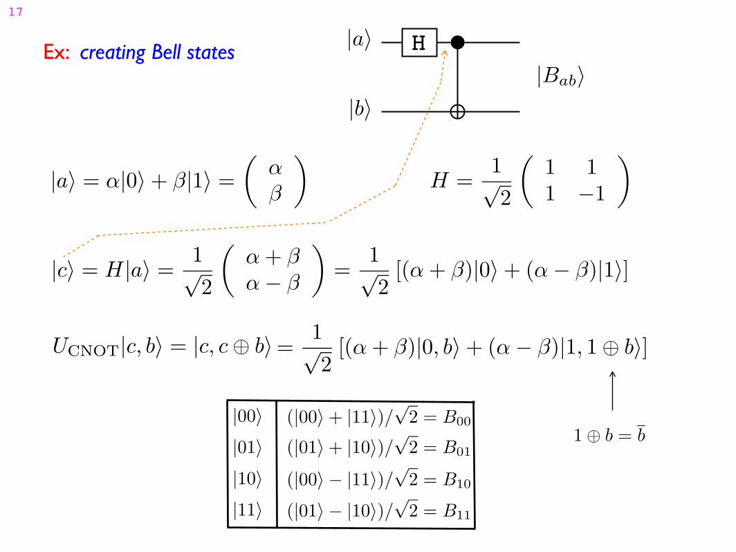
Ex: creating Bell states H|a〉
|b〉
|Bab〉
|a〉 = α|0〉 + β|1〉 =
(αβ
)H =
1√
2
(1 1
1 −1
)
UCNOT|c, b〉 = |c, c ⊕ b〉=1√2
[(α + β)|0, b〉 + (α − β)|1, 1 ⊕ b〉]
|c〉 = H|a〉 =1√2
(α + βα − β
)=
1√2
[(α + β)|0〉 + (α − β)|1〉]
1 ⊕ b = b
|00〉
|01〉
|10〉
|11〉 (|01〉 − |10〉)/√2 = B11
(|00〉 + |11〉)/√2 = B00
(|00〉 − |11〉)/√2 = B10
(|01〉 + |10〉)/√2 = B01
17
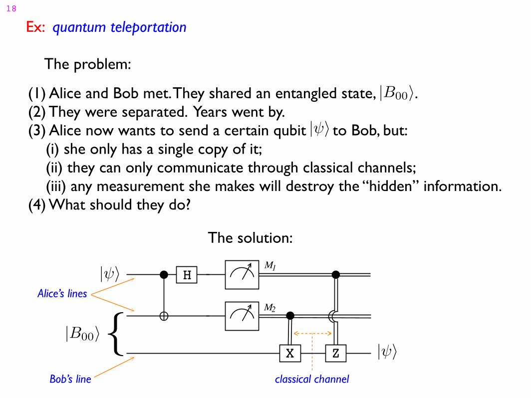
Ex: quantum teleportation
The problem:
(1) Alice and Bob met. They shared an entangled state, .(2) They were separated. Years went by.(3) Alice now wants to send a certain qubit to Bob, but: (i) she only has a single copy of it; (ii) they can only communicate through classical channels; (iii) any measurement she makes will destroy the “hidden” information.(4) What should they do?
|B00〉
|ψ〉
Alice’s lines
Bob’s line classical channel
|ψ〉
2
H
X Z
M
M
1
|B00〉{|ψ〉
The solution:
18
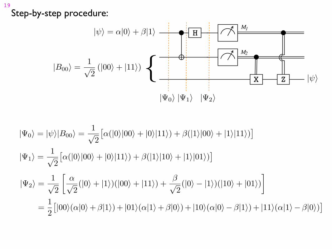
Step-by-step procedure:
|Ψ0〉 |Ψ1〉 |Ψ2〉
|ψ〉
|B00〉 =1√2
(|00〉 + |11〉)2
H
X Z
M
M
1
{
|ψ〉 = α|0〉 + β|1〉
=1
2
[|00〉(α|0〉+β|1〉)+ |01〉(α|1〉+β|0〉)+ |10〉(α|0〉−β|1〉)+ |11〉(α|1〉−β|0〉)
]
|Ψ1〉 =1√2
[α(|0〉|00〉 + |0〉|11〉) + β(|1〉|10〉 + |1〉|01〉)]
|Ψ2〉 =1√2
[α√2(|0〉 + |1〉)(|00〉 + |11〉) +
β√2(|0〉 − |1〉)(|10〉 + |01〉)
]
|Ψ0〉 = |ψ〉|B00〉 =1√2
[α(|0〉|00〉 + |0〉|11〉) + β(|1〉|00〉 + |1〉|11〉)]
19
Step-by-step procedure:
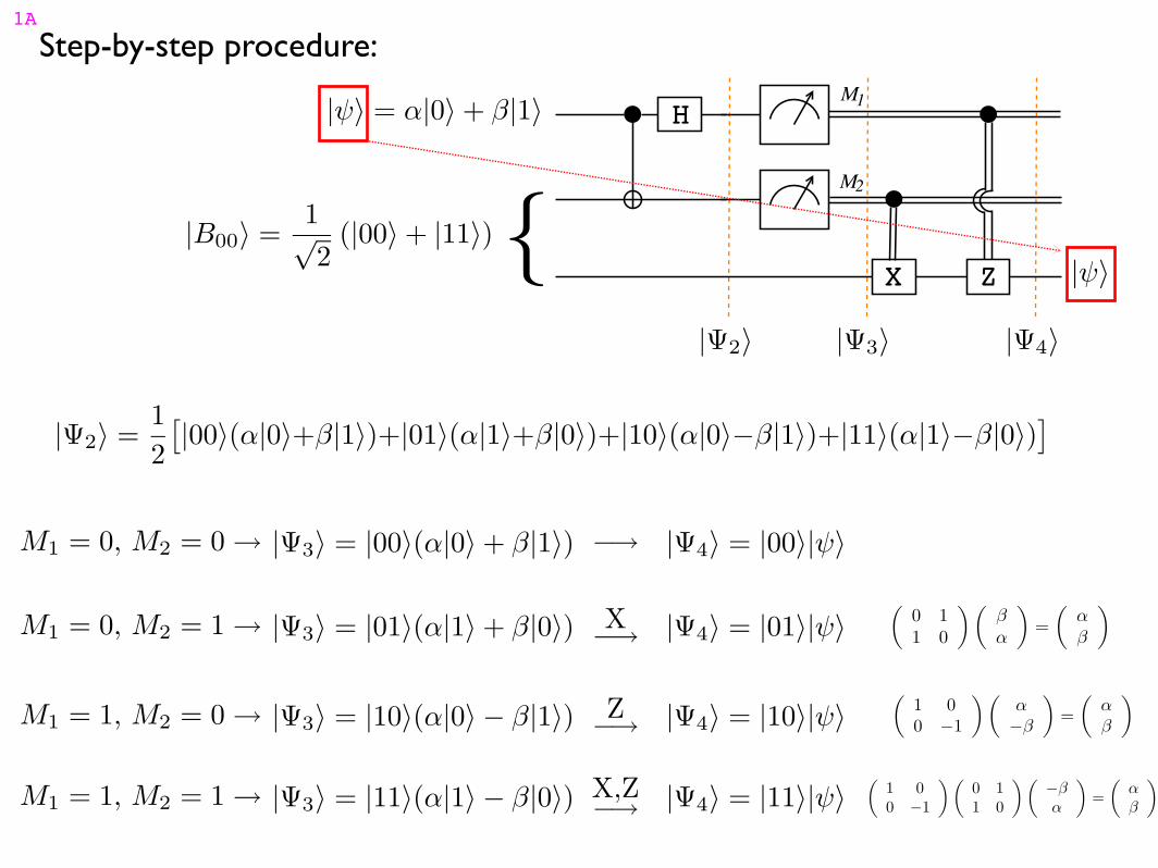
|Ψ2〉 |Ψ3〉 |Ψ4〉
|ψ〉
|B00〉 =1√2
(|00〉 + |11〉)2
H
X Z
M
M
1
{
|ψ〉 = α|0〉 + β|1〉
|Ψ2〉 =1
2
[|00〉(α|0〉+β|1〉)+|01〉(α|1〉+β|0〉)+|10〉(α|0〉−β|1〉)+|11〉(α|1〉−β|0〉)
]
|Ψ3〉 = |00〉(α|0〉 + β|1〉)M1 = 0, M2 = 0 → −→ |Ψ4〉 = |00〉|ψ〉
|Ψ3〉 = |01〉(α|1〉 + β|0〉)M1 = 0, M2 = 1 →
|Ψ3〉 = |10〉(α|0〉 − β|1〉)M1 = 1, M2 = 0 →
|Ψ3〉 = |11〉(α|1〉 − β|0〉)M1 = 1, M2 = 1 →
X−→
|Ψ4〉 = |01〉|ψ〉(
0 1
1 0
) (βα
)=
(αβ
)
Z−→
|Ψ4〉 = |10〉|ψ〉(
1 0
0 −1
) (α−β
)=
(αβ
)
X,Z−→
|Ψ4〉 = |11〉|ψ〉(
1 0
0 −1
)(0 1
1 0
)(−βα
)=
(αβ
)
1A
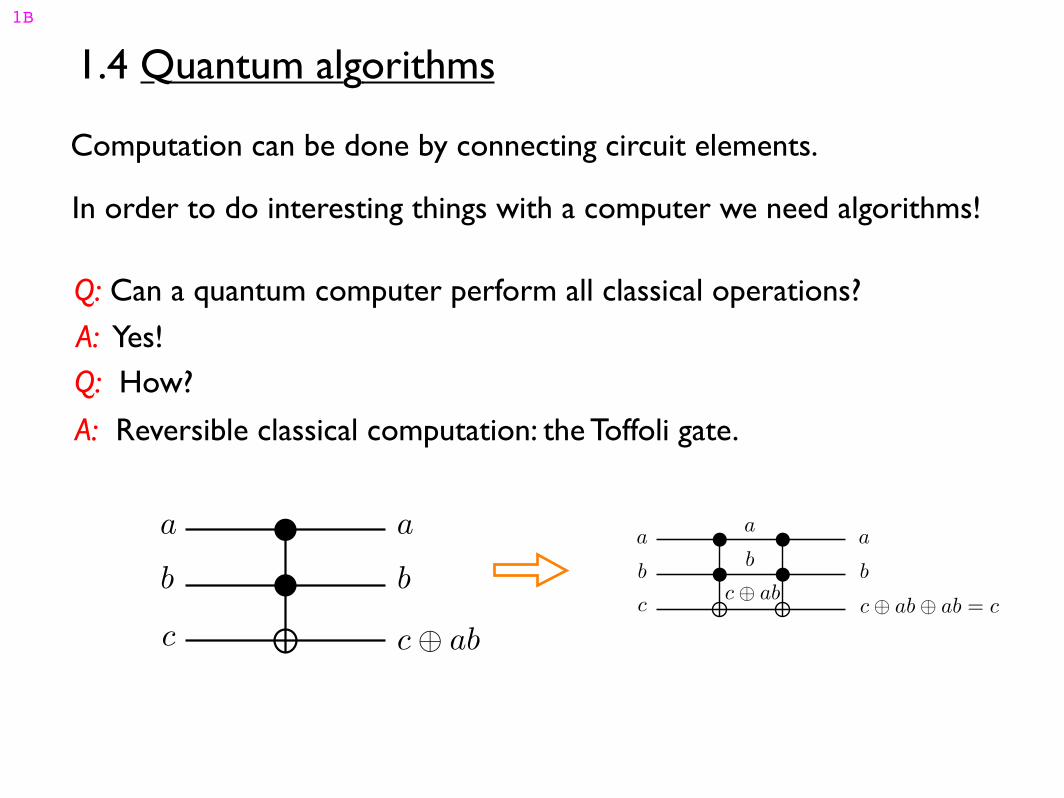
1.4 Quantum algorithms
In order to do interesting things with a computer we need algorithms!
Computation can be done by connecting circuit elements.
Q: Can a quantum computer perform all classical operations?
A: Yes!Q: How?
A: Reversible classical computation: the Toffoli gate.
a
b
c c ⊕ ab
b
a
c ⊕ ab
a
b
c
a
bb
a
c ⊕ ab ⊕ ab = c
1B
a
0
1
b
0
0
c
0
0
a′
0
b′
0
0
c′
0
0
10 0 0 0
1
1
10 0 0 0 1
1 0 11 1 1
1
01 0 11 1
010 11 1
1 011 1
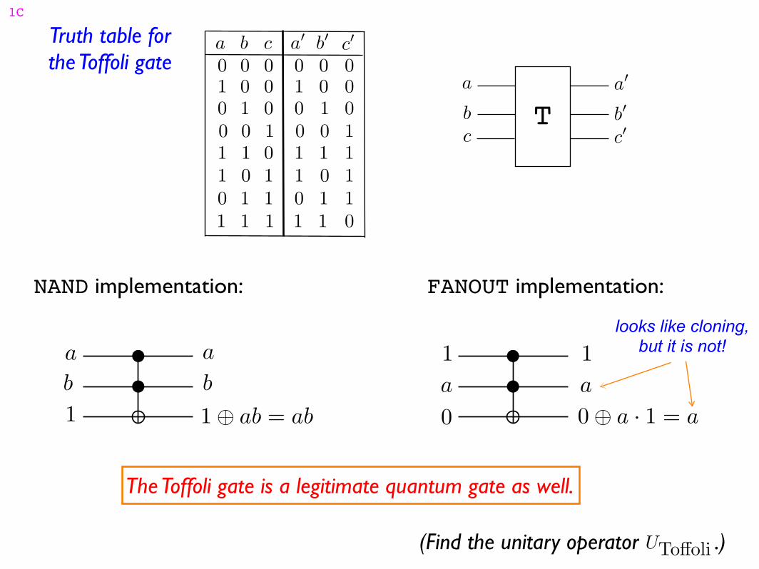
Truth table forthe Toffoli gate
Tc
a
b b′
a′
c′
NAND implementation:
a a
b b
1 1 ⊕ ab = ab
FANOUT implementation:
a a
1
0 ⊕ a · 1 = a0
1
(Find the unitary operator .)UToffoli
The Toffoli gate is a legitimate quantum gate as well.
looks like cloning,but it is not!
1C
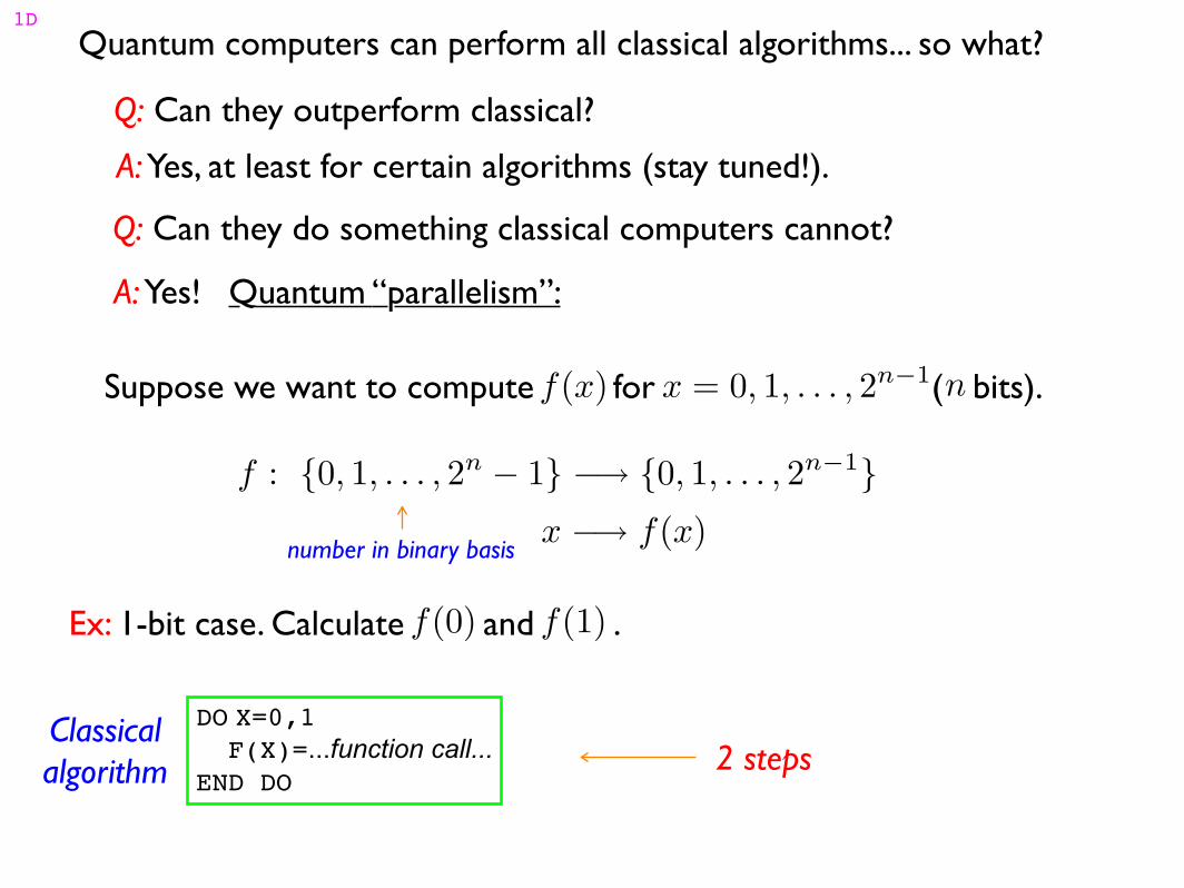
Quantum computers can perform all classical algorithms... so what?
Q: Can they do something classical computers cannot?
Quantum “parallelism”: A: Yes!
Suppose we want to compute for ( bits).f(x) x = 0, 1, . . . , 2n−1
n
f : {0, 1, . . . , 2n − 1} −→ {0, 1, . . . , 2n−1}
x −→ f(x)
Ex: 1-bit case. Calculate and .f(0) f(1)
number in binary basis
DO X=0,1 F(X)=...function call...END DO
Classicalalgorithm 2 steps
Q: Can they outperform classical?
A: Yes, at least for certain algorithms (stay tuned!).
1D
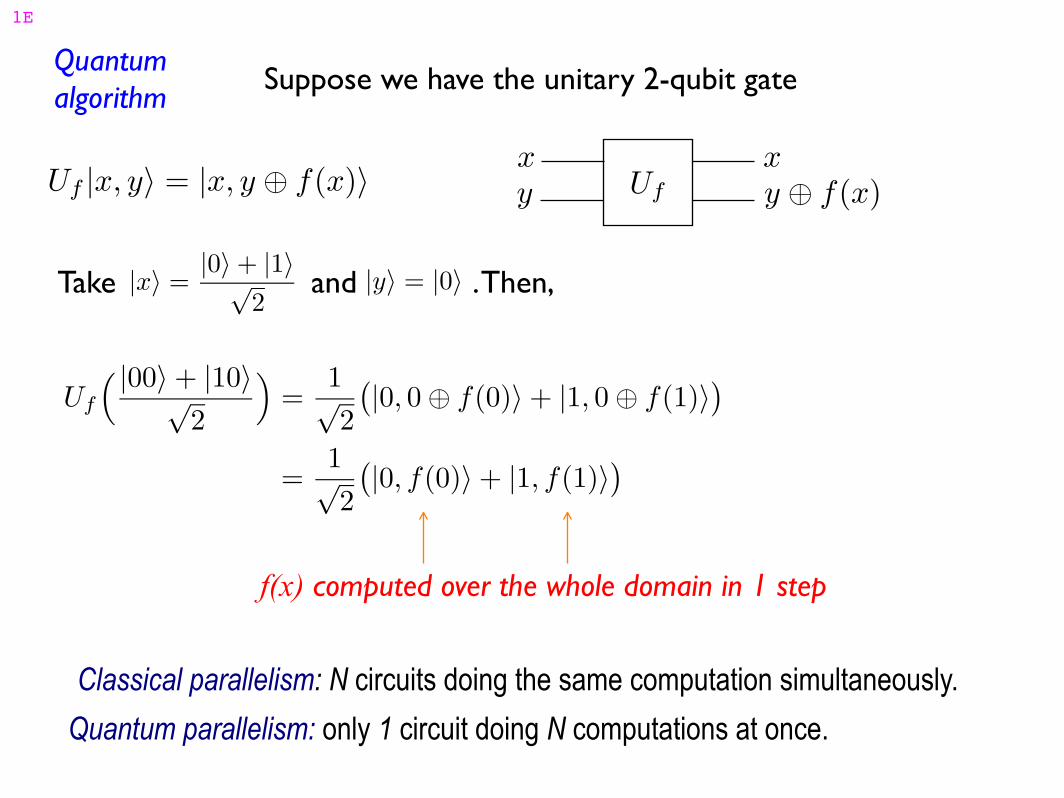
Quantumalgorithm
Suppose we have the unitary 2-qubit gate
Uf
x
y
x
y ⊕ f(x)Uf |x, y〉 = |x, y ⊕ f(x)〉
Take and . Then,|x〉 =|0〉 + |1〉√
2|y〉 = |0〉
Uf
( |00〉 + |10〉√2
)=
1√2
(|0, 0 ⊕ f(0)〉 + |1, 0 ⊕ f(1)〉)
=1√2
(|0, f(0)〉 + |1, f(1)〉)
f(x) computed over the whole domain in 1 step
Quantum parallelism: only 1 circuit doing N computations at once.
Classical parallelism: N circuits doing the same computation simultaneously.
1E
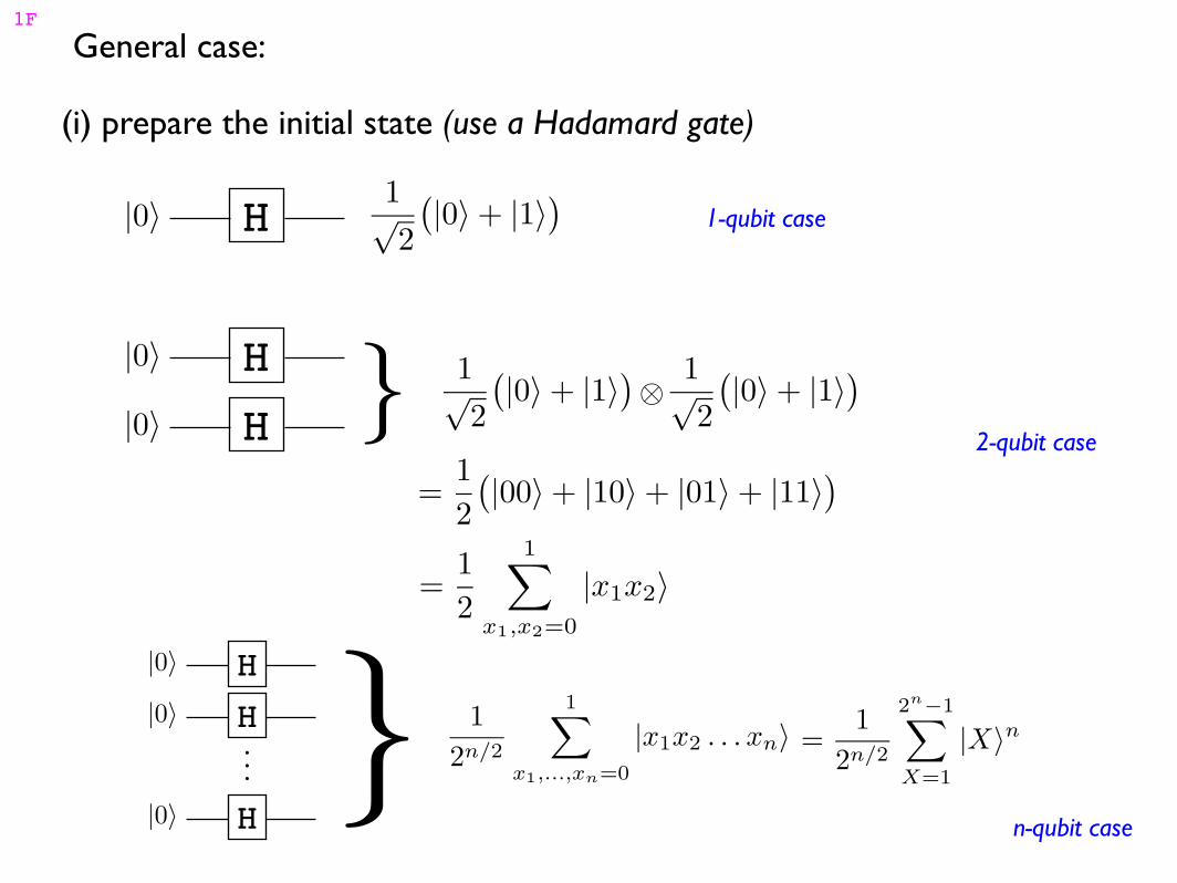
General case:
(i) prepare the initial state (use a Hadamard gate)
|0〉1√2
(|0〉 + |1〉)H 1-qubit case
=1
2
(|00〉 + |10〉 + |01〉 + |11〉
)
|0〉 H|0〉 H } 1√
2
(|0〉 + |1〉) 1√2
(|0〉 + |1〉)⊗
2-qubit case
=1
2
1∑
x1,x2=0
|x1x2〉
HH.
.
.
H
|0〉
|0〉
|0〉
} 1
2n/2
1∑
x1,...,xn=0
|x1x2 . . . xn〉
n-qubit case
=1
2n/2
2n−1∑
X=1
|X〉n
1F
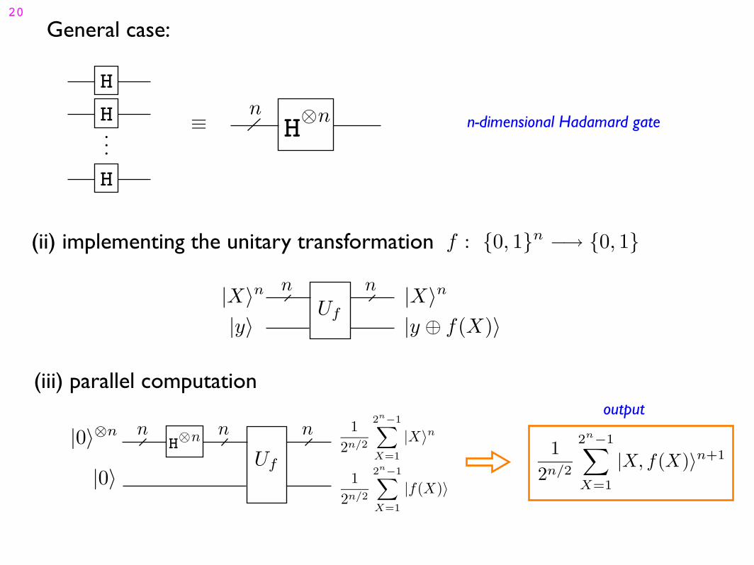
General case:
HH.
.
.
H
≡⊗H n
nn-dimensional Hadamard gate
(iii) parallel computation
H n⊗
Uf
|0〉⊗n
|0〉
n n n 1
2n/2
2n−1∑
X=1
|X〉n
1
2n/2
2n−1∑
X=1
|f(X)〉
1
2n/2
2n−1∑
X=1
|X, f(X)〉n+1
output
(ii) implementing the unitary transformation f : {0, 1}n −→ {0, 1}
Uf
n n
|y ⊕ f(X)〉|y〉
|X〉n|X〉n
20
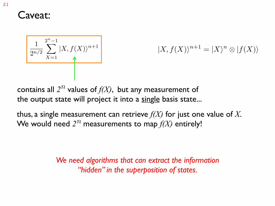
Caveat:
1
2n/2
2n−1∑
X=1
|X, f(X)〉n+1 |X, f(X)〉n+1 = |X〉n ⊗ |f(X)〉
contains all 2 values of f(X), but any measurement of the output state will project it into a single basis state...
n
thus, a single measurement can retrieve f(X) for just one value of X. We would need 2 measurements to map f(X) entirely!n
We need algorithms that can extract the information “hidden” in the superposition of states.
21
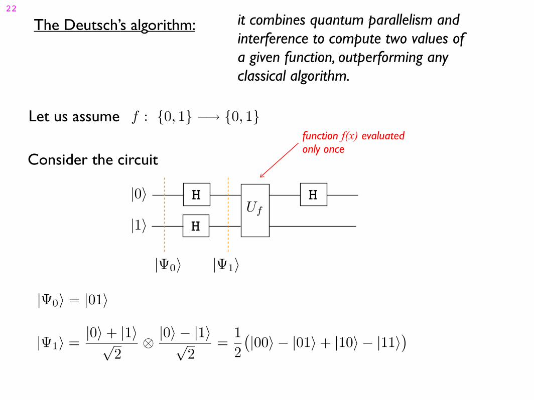
The Deutsch’s algorithm: it combines quantum parallelism and interference to compute two values of a given function, outperforming any classical algorithm.
Let us assume f : {0, 1} −→ {0, 1}
Consider the circuit
Uf
H|0〉
H|1〉
H
|Ψ0〉 |Ψ1〉
|Ψ0〉 = |01〉
function f(x) evaluated only once
|Ψ1〉 =|0〉 + |1〉√
2⊗ |0〉 − |1〉√
2=
1
2
(|00〉 − |01〉 + |10〉 − |11〉)
22
Uf
H|0〉
H|1〉
H
|Ψ2〉 |Ψ3〉
1 ⊕ x = x
0 ⊕ x = x|Ψ2〉 =
1
2
(|0, f(0)〉 −
∣∣0, f(0)⟩
+ |1, f(1)〉 −∣∣1, f(1)
⟩).
|Ψ3〉 =1
2
(|0, f(0)〉 + |1, f(0)〉√
2−
∣∣0, f(0)⟩
+∣∣1, f(0)
⟩√
2
+|0, f(1)〉 − |1, f(1)〉√
2−
∣∣0, f(1)⟩ − ∣∣1, f(1)
⟩√
2
)
.
=1√8
[|0〉 ⊗
(|f(0)〉 + |f(1)〉 − ∣∣f(0)
⟩ − ∣∣f(1)⟩)
+ |1〉 ⊗(|f(0)〉 − |f(1)〉 −
∣∣f(0)⟩
+∣∣f(1)
⟩)]
23
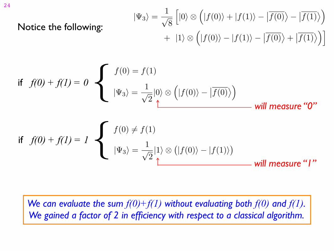
Notice the following: + |1〉 ⊗
(|f(0)〉 − |f(1)〉 −
∣∣f(0)⟩
+∣∣f(1)
⟩)]|Ψ3〉 =
1√8
[|0〉 ⊗
(|f(0)〉 + |f(1)〉 − ∣∣f(0)
⟩ − ∣∣f(1)⟩)
|Ψ3〉 =1√2|1〉 ⊗ (|f(0)〉 − |f(1)〉)
f(0) != f(1)
if f(0) + f(1) = 1{
if f(0) + f(1) = 0f(0) = f(1)
|Ψ3〉 =1√2|0〉 ⊗
(|f(0)〉 − ∣∣f(0)
⟩){will measure “0”
will measure “1”
We can evaluate the sum f(0)+f(1) without evaluating both f(0) and f(1). We gained a factor of 2 in efficiency with respect to a classical algorithm.
24
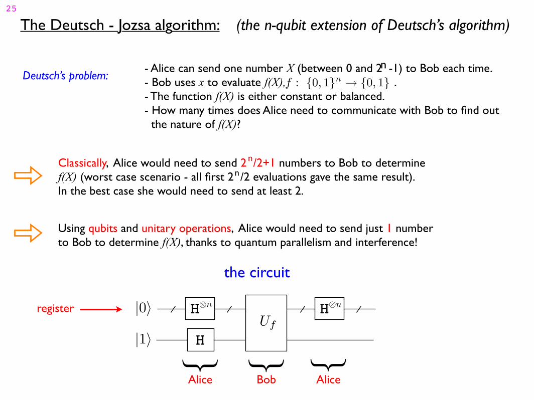
The Deutsch - Jozsa algorithm: (the n-qubit extension of Deutsch’s algorithm)
Deutsch’s problem:- Alice can send one number X (between 0 and 2 -1) to Bob each time.- Bob uses x to evaluate f(X), .- The function f(X) is either constant or balanced.- How many times does Alice need to communicate with Bob to find out the nature of f(X)?
f : {0, 1}n → {0, 1}
n
Classically, Alice would need to send 2 /2+1 numbers to Bob to determine f(X) (worst case scenario - all first 2 /2 evaluations gave the same result). In the best case she would need to send at least 2.
n
n
Using qubits and unitary operations, Alice would need to send just 1 number to Bob to determine f(X), thanks to quantum parallelism and interference!
the circuit
|0〉
|1〉Uf
H
H⊗n H⊗nregister
} } }
Alice AliceBob
25
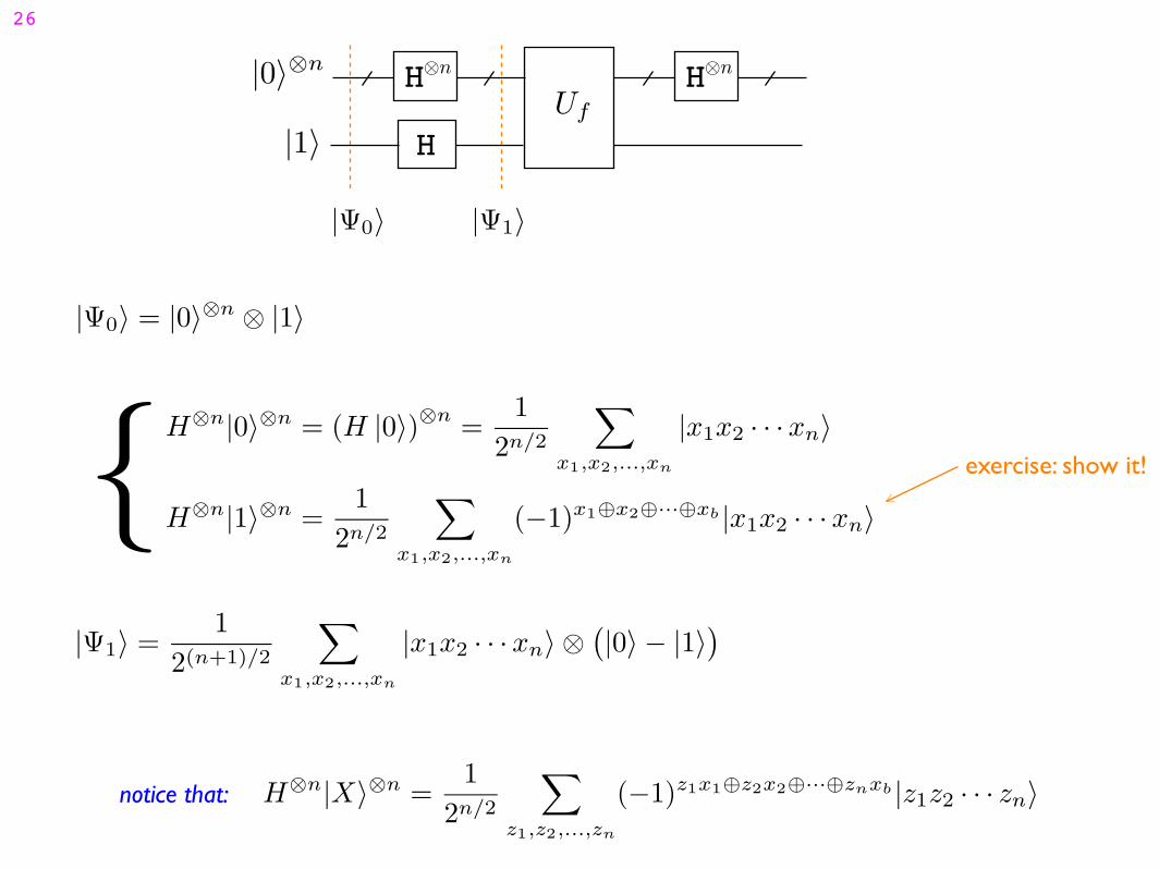
|Ψ0〉 |Ψ1〉
|1〉Uf
H
H⊗n H⊗n|0〉⊗n
|Ψ0〉 = |0〉⊗n ⊗ |1〉
|Ψ1〉 =1
2(n+1)/2
∑
x1,x2,...,xn
|x1x2 · · ·xn〉 ⊗(|0〉 − |1〉
)
H⊗n|0〉⊗n = (H |0〉)⊗n =
1
2n/2
∑
x1,x2,...,xn
|x1x2 · · ·xn〉{H
⊗n|1〉⊗n =1
2n/2
∑
x1,x2,...,xn
(−1)x1⊕x2⊕···⊕xb |x1x2 · · ·xn〉
notice that: H⊗n|X〉⊗n =
1
2n/2
∑
z1,z2,...,zn
(−1)z1x1⊕z2x2⊕···⊕znxb |z1z2 · · · zn〉
exercise: show it!
26
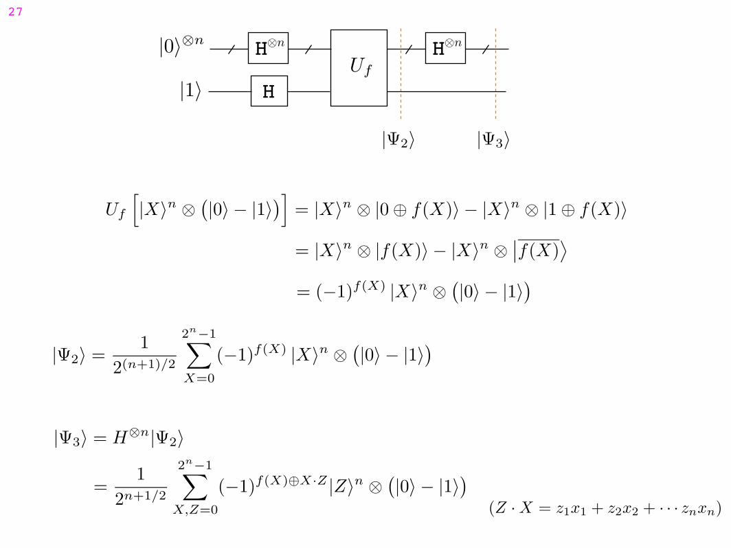
|Ψ2〉 |Ψ3〉
|1〉Uf
H
H⊗n H⊗n|0〉⊗n
Uf
[|X〉n ⊗
(|0〉 − |1〉
)]= |X〉n ⊗ |0 ⊕ f(X)〉 − |X〉n ⊗ |1 ⊕ f(X)〉
= |X〉n ⊗ |f(X)〉 − |X〉n ⊗∣∣f(X)
⟩
= (−1)f(X) |X〉n ⊗(|0〉 − |1〉
)
|Ψ2〉 =1
2(n+1)/2
2n−1∑
X=0
(−1)f(X) |X〉n ⊗(|0〉 − |1〉
)
|Ψ3〉 = H⊗n|Ψ2〉
(Z · X = z1x1 + z2x2 + · · · znxn)=
1
2n+1/2
2n−1∑
X,Z=0
(−1)f(X)⊕X·Z |Z〉n ⊗(|0〉 − |1〉
)
27

{
|Ψ3〉 =2n
−1∑
X,Z=0
(−1)f(X)⊕X·Z
2n|Z〉n ⊗ |0〉 − |1〉√
2
A(X, Z)
|Ψ3| = 1But |Ψ3〉 = |0〉⊗n ⊗ |0〉 − |1〉√2
|0〉⊗nThe state has zero amplitude at least one qubit will be |1〉
If Alice measures at least one qubit in the state “1”, the function is balanced; otherwise it is constant.
constant f(X): 2n
−1∑
X=0
A(X, 0) =2n
−1∑
X=0
(−1)f(X)
2n= ±1
(Z = 0)
balanced f(X): 2n
−1∑
X=0
A(X, 0) =2n
−1∑
X=0
(−1)f(X)
2n=
(−1)0 + (−1)1
2= 0
(Z = 0)
28
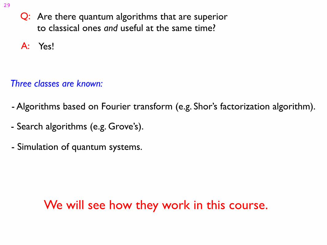
Are there quantum algorithms that are superiorto classical ones and useful at the same time?
Q:
Yes!A:
- Algorithms based on Fourier transform (e.g. Shor’s factorization algorithm).
- Search algorithms (e.g. Grove’s).
- Simulation of quantum systems.
Three classes are known:
We will see how they work in this course.
29
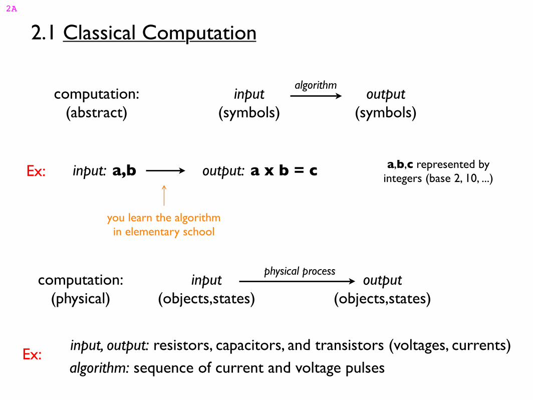
2.1 Classical Computation
Ex: input: a,b output: a x b = c a,b,c represented byintegers (base 2, 10, ...)
computation:(abstract)
input(symbols)
output(symbols)
algorithm
you learn the algorithmin elementary school
computation:(physical)
input(objects,states)
output(objects,states)
physical process
Ex:input, output: resistors, capacitors, and transistors (voltages, currents)algorithm: sequence of current and voltage pulses
2A
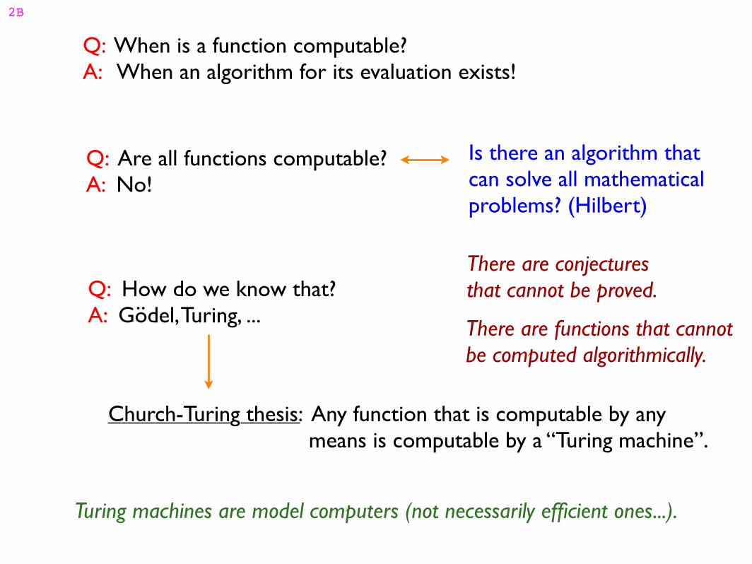
Q: When is a function computable?A: When an algorithm for its evaluation exists!
Q: Are all functions computable?A: No!
..Q: How do we know that?A: Godel, Turing, ...
Church-Turing thesis: Any function that is computable by any means is computable by a “Turing machine”.
There are conjecturesthat cannot be proved.
There are functions that cannotbe computed algorithmically.
Turing machines are model computers (not necessarily efficient ones...).
2B
Is there an algorithm thatcan solve all mathematicalproblems? (Hilbert)
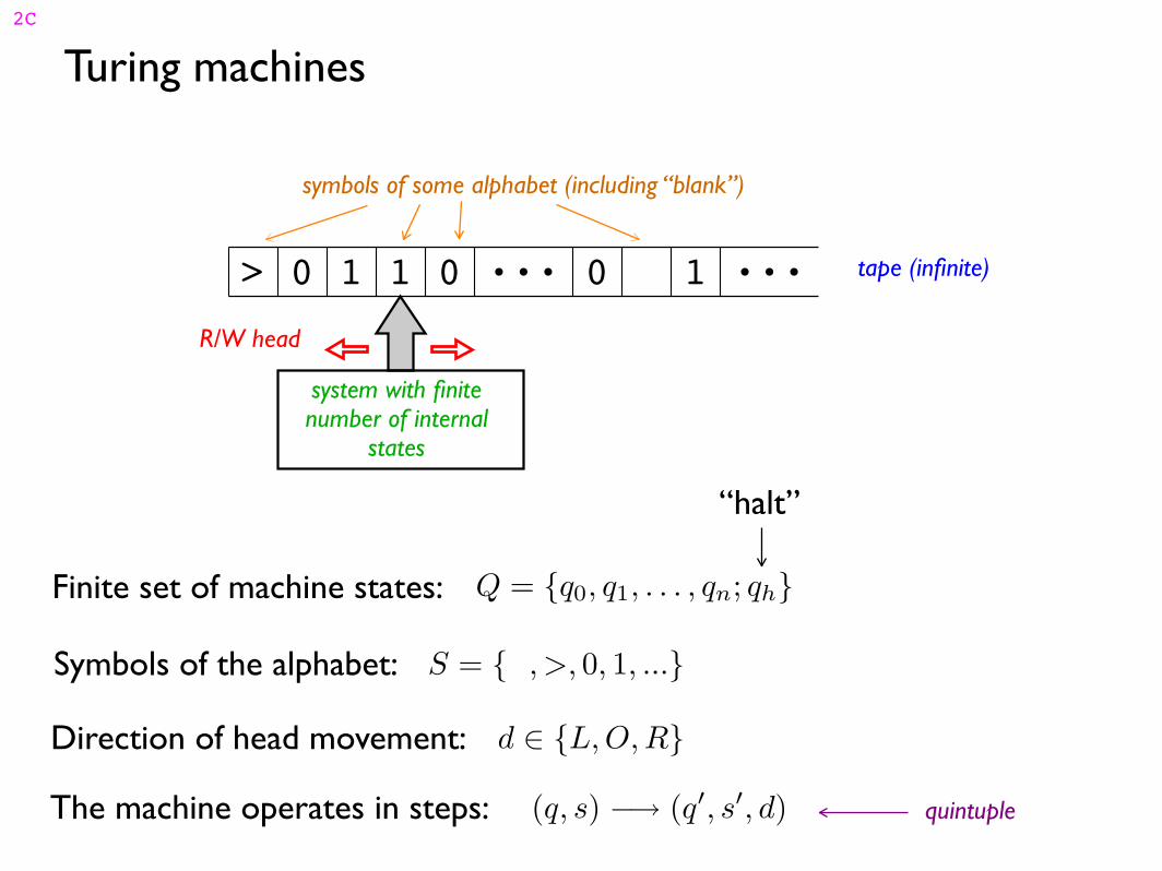
Turing machines2C
tape (infinite)1> 0 1 1 0 0
R/W head
system with finitenumber of internal
states
symbols of some alphabet (including “blank”)
Q = {q0, q1, . . . , qn; qh}Finite set of machine states:
“halt”
Symbols of the alphabet: S = { , >, 0, 1, ...}
Direction of head movement: d ∈ {L, O, R}
quintupleThe machine operates in steps: (q, s) −→ (q′, s′, d)
2D
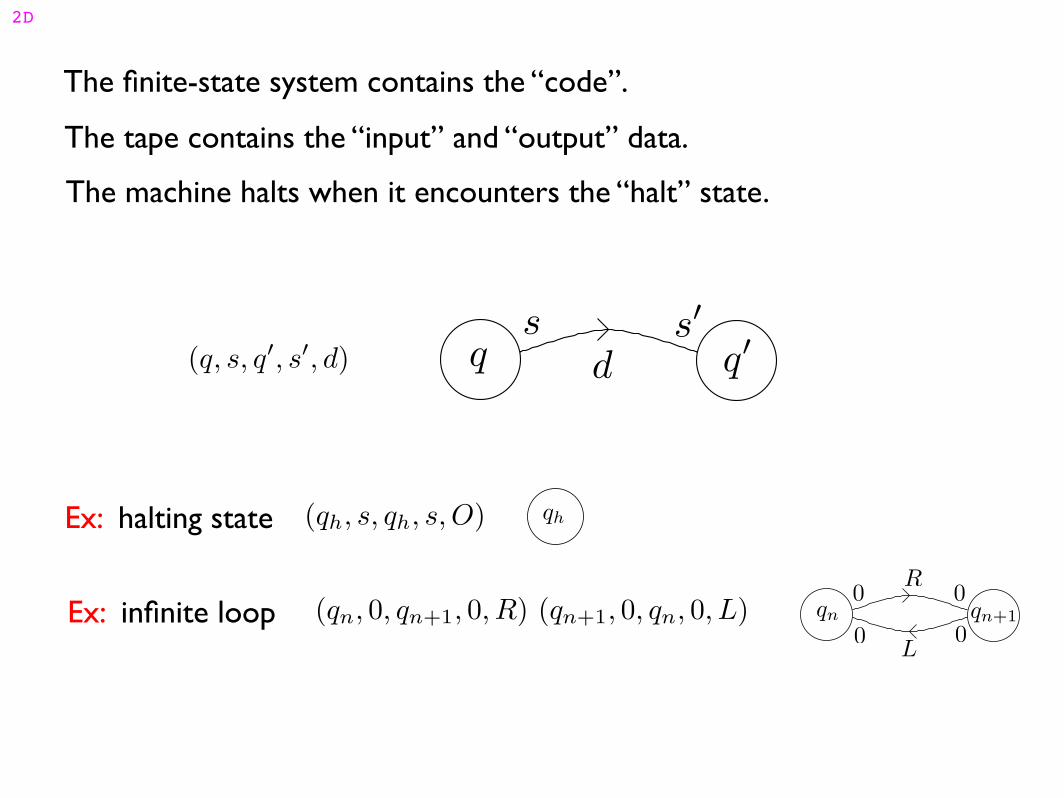
The finite-state system contains the “code”.
The tape contains the “input” and “output” data.
The machine halts when it encounters the “halt” state.
(q, s, q′, s′, d) q q′
s′
s
d
Ex: infinite loop (qn, 0, qn+1, 0, R) (qn+1, 0, qn, 0, L) qn+1qn
0 0
0 0
R
L
(qh, s, qh, s, O)Ex: halting state qh
2E
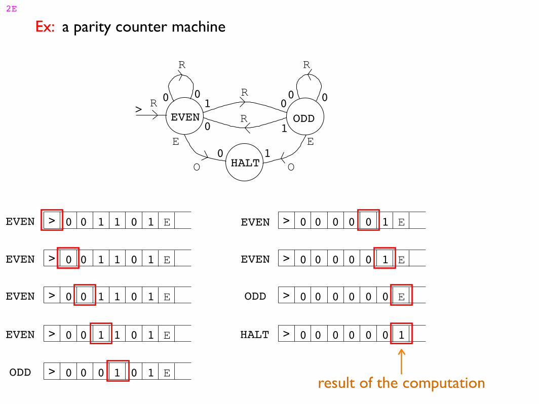
Ex: a parity counter machine
EVEN ODD
HALT
> RR
R
O O
E E0 1
1 0
0 1
0 0 0 0
R R
> 0 0 1 1 10 EEVEN
> 0 0 1 1 10 EEVEN
> 0 0 1 1 10 EEVEN
> 0 0 1 1 10 EEVEN
> 0 0 0 1 10 EODD
> 0 0 0 0 00 EODD
> 0 0 0 0 10 EEVEN
> 0 0 0 0 10 EEVEN
> 0 0 0 0 00 1HALT
result of the computation
2F
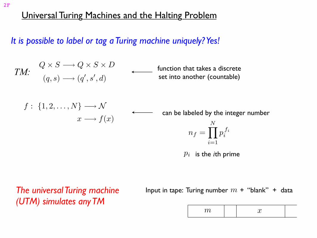
Universal Turing Machines and the Halting Problem
It is possible to label or tag a Turing machine uniquely? Yes!
Q × S −→ Q × S × D
(q, s) −→ (q′, s′, d)TM: function that takes a discrete
set into another (countable)
f : {1, 2, . . . , N} −→ N
x −→ f(x)can be labeled by the integer number
nf =
N∏
i=1
pfi
i
pi is the ith prime
The universal Turing machine (UTM) simulates any TM
Input in tape: Turing number + “blank” + data
xm
m
30
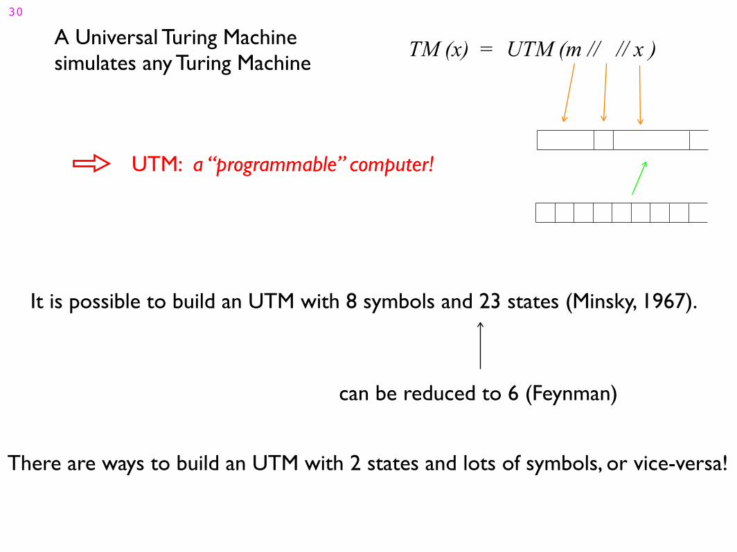
A Universal Turing Machinesimulates any Turing Machine
TM (x) = UTM (m // // x )
UTM: a “programmable” computer!
It is possible to build an UTM with 8 symbols and 23 states (Minsky, 1967).
can be reduced to 6 (Feynman)
There are ways to build an UTM with 2 states and lots of symbols, or vice-versa!
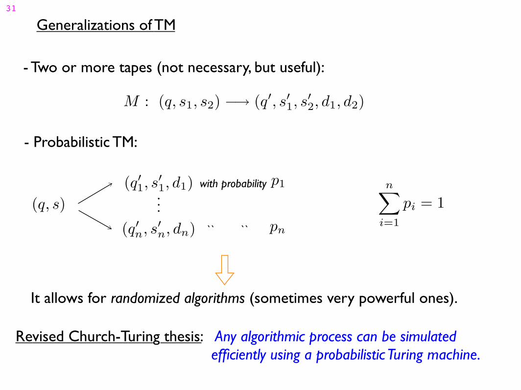
Generalizations of TM31
- Two or more tapes (not necessary, but useful):
M : (q, s1, s2) −→ (q′, s′1, s′
2, d1, d2)
- Probabilistic TM:
(q, s)
(q′1, s′
1, d1)
(q′n, s′
n, dn)
.
.
.
p1
pn
n∑
i=1
pi = 1
with probability
`` ``
It allows for randomized algorithms (sometimes very powerful ones).
Revised Church-Turing thesis: Any algorithmic process can be simulated efficiently using a probabilistic Turing machine.
32
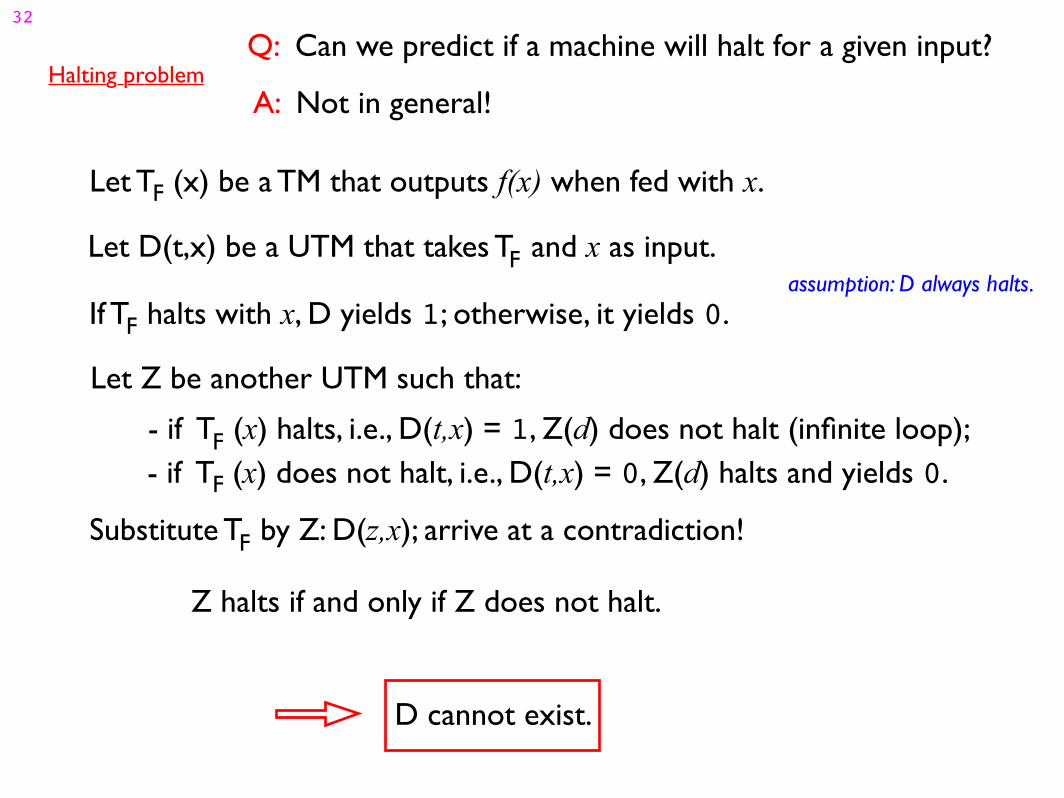
Let Z be another UTM such that:
F- if T (x) halts, i.e., D(t,x) = 1, Z(d) does not halt (infinite loop);- if T (x) does not halt, i.e., D(t,x) = 0, Z(d) halts and yields 0.F
Substitute T by Z: D(z,x); arrive at a contradiction!F
Z halts if and only if Z does not halt.
Q: Can we predict if a machine will halt for a given input?
A: Not in general!
Let T (x) be a TM that outputs f(x) when fed with x.F
Let D(t,x) be a UTM that takes T and x as input.F
If T halts with x, D yields 1; otherwise, it yields 0.F
assumption: D always halts.
D cannot exist.
Halting problem
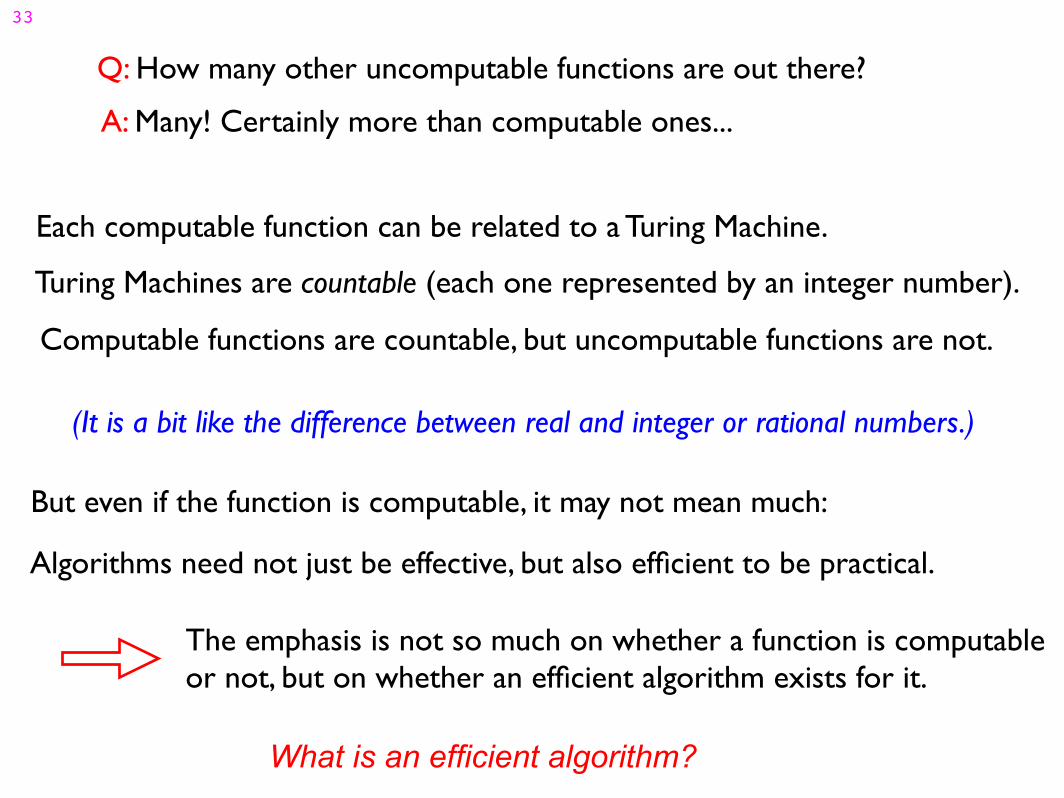
Q: How many other uncomputable functions are out there?
A: Many! Certainly more than computable ones...
Each computable function can be related to a Turing Machine.
Turing Machines are countable (each one represented by an integer number).
Computable functions are countable, but uncomputable functions are not.
(It is a bit like the difference between real and integer or rational numbers.)
But even if the function is computable, it may not mean much:
Algorithms need not just be effective, but also efficient to be practical.
The emphasis is not so much on whether a function is computable or not, but on whether an efficient algorithm exists for it.
What is an efficient algorithm?
33
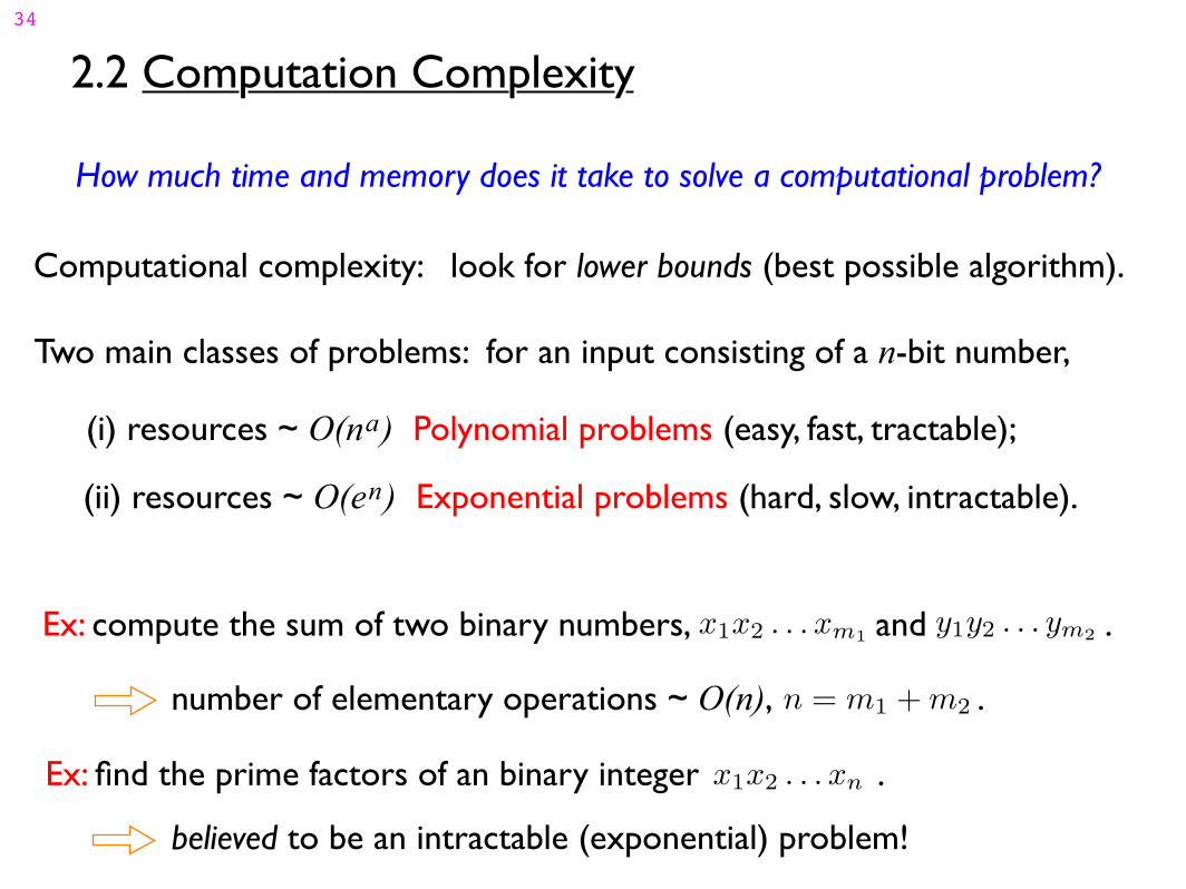
2.2 Computation Complexity34
How much time and memory does it take to solve a computational problem?
Computational complexity: look for lower bounds (best possible algorithm).
Two main classes of problems: for an input consisting of a n-bit number,
(i) resources ~ O(n ) Polynomial problems (easy, fast, tractable);a
(ii) resources ~ O(e ) Exponential problems (hard, slow, intractable).n
Ex: compute the sum of two binary numbers, and .x1x2 . . . xm1y1y2 . . . ym2
number of elementary operations ~ O(n), .n = m1 + m2
Ex: find the prime factors of an binary integer . x1x2 . . . xn
believed to be an intractable (exponential) problem!
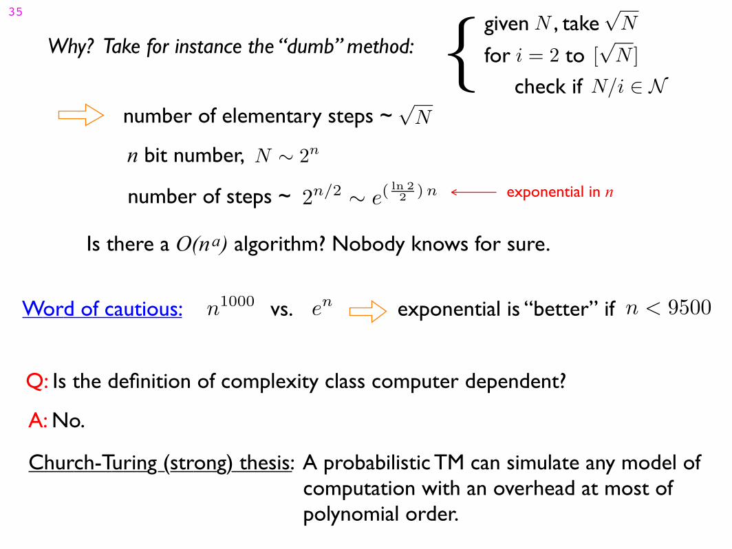
Why? Take for instance the “dumb” method:
35given , take N
√N
i = 2 [√
N ]for to check if N/i ∈ N
{√
Nnumber of elementary steps ~
n bit number, N ∼ 2n
2n/2
∼ e( ln 2
2) nnumber of steps ~ exponential in n
Is there a O(n ) algorithm? Nobody knows for sure.a
Word of cautious: n1000
envs. exponential is “better” if n < 9500
Q: Is the definition of complexity class computer dependent?
A: No.
Church-Turing (strong) thesis: A probabilistic TM can simulate any model of computation with an overhead at most of polynomial order.
2.3 Complexity Classes35
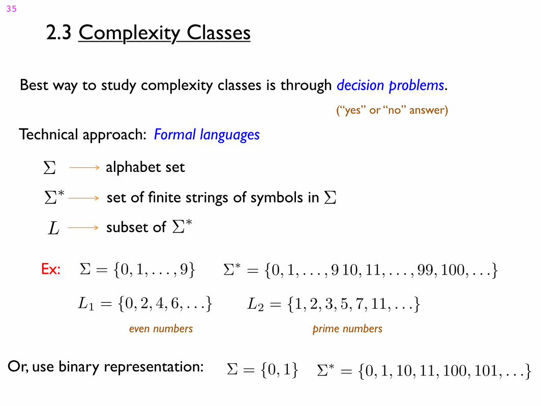
Best way to study complexity classes is through decision problems.
(“yes” or “no” answer)
Technical approach: Formal languages
Σ alphabet set
Σ∗ set of finite strings of symbols in Σ
L subset of Σ∗
Ex: Σ = {0, 1, . . . , 9} Σ∗
= {0, 1, . . . , 9 10, 11, . . . , 99, 100, . . .}
L1 = {0, 2, 4, 6, . . .} L2 = {1, 2, 3, 5, 7, 11, . . .}
even numbers prime numbers
Or, use binary representation: Σ = {0, 1} Σ∗
= {0, 1, 10, 11, 100, 101, . . .}
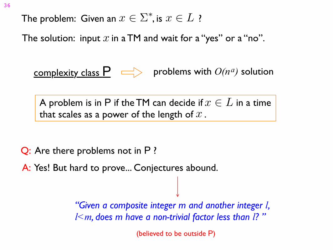
Q: Are there problems not in P ?
A: Yes! But hard to prove... Conjectures abound.
problems with O(n ) solutionacomplexity class P
The problem: Given an , is ?x ∈ Σ∗
x ∈ L
The solution: input in a TM and wait for a “yes” or a “no”. x
A problem is in P if the TM can decide if in a timethat scales as a power of the length of .
x ∈ L
x
“Given a composite integer m and another integer l, l<m, does m have a non-trivial factor less than l? ”
(believed to be outside P)
36
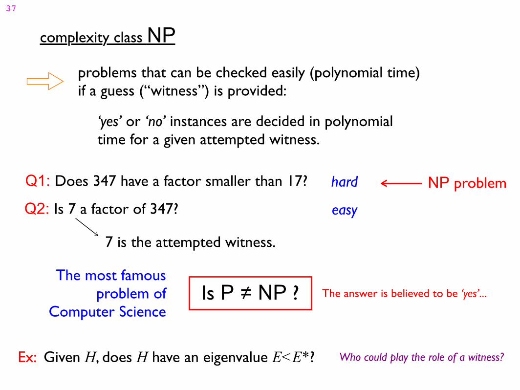
complexity class NP
Q1: Does 347 have a factor smaller than 17?
Q2: Is 7 a factor of 347?
hard
easy
‘yes’ or ‘no’ instances are decided in polynomial time for a given attempted witness.
37
problems that can be checked easily (polynomial time) if a guess (“witness”) is provided:
NP problem
7 is the attempted witness.
The most famousproblem of
Computer ScienceIs P = NP ? The answer is believed to be ‘yes’...
Ex: Given H, does H have an eigenvalue E<E*? Who could play the role of a witness?
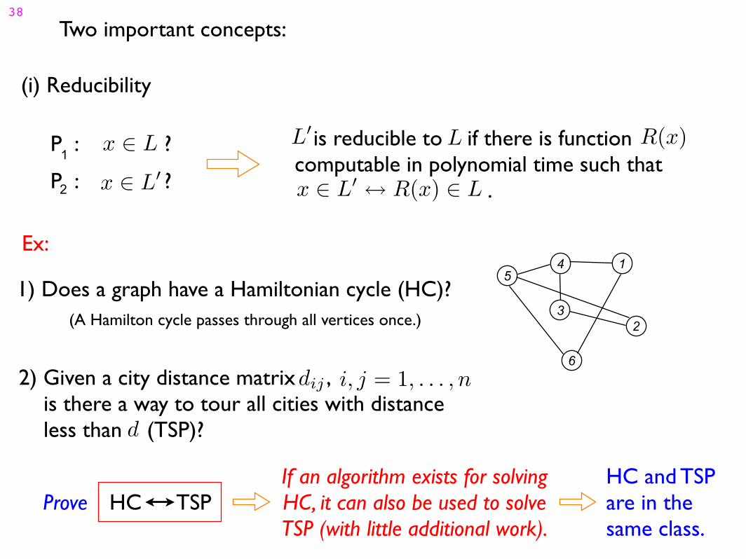
38Two important concepts:
(i) Reducibility
P : ?1
P : ?2
x ∈ L
x ∈ L′
is reducible to if there is function computable in polynomial time such that .
L′
L
x ∈ L′↔ R(x) ∈ L
R(x)
Ex:1
6
54
32
1) Does a graph have a Hamiltonian cycle (HC)?(A Hamilton cycle passes through all vertices once.)
2) Given a city distance matrix , is there a way to tour all cities with distance less than (TSP)?
dij
d
i, j = 1, . . . , n
HC TSPProve If an algorithm exists for solvingHC, it can also be used to solve TSP (with little additional work).
HC and TSPare in the same class.
39
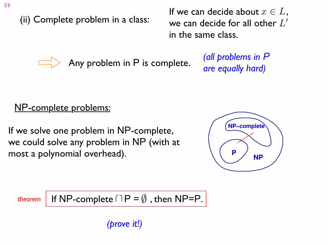
(ii) Complete problem in a class:If we can decide about ,we can decide for all other in the same class.
x ∈ L
L′
Any problem in P is complete.(all problems in Pare equally hard)
NP-complete problems:
If NP-complete P = , then NP=P. ∩ ∅theorem
(prove it!)
If we solve one problem in NP-complete, we could solve any problem in NP (with atmost a polynomial overhead). P
NP
NP−complete
3A
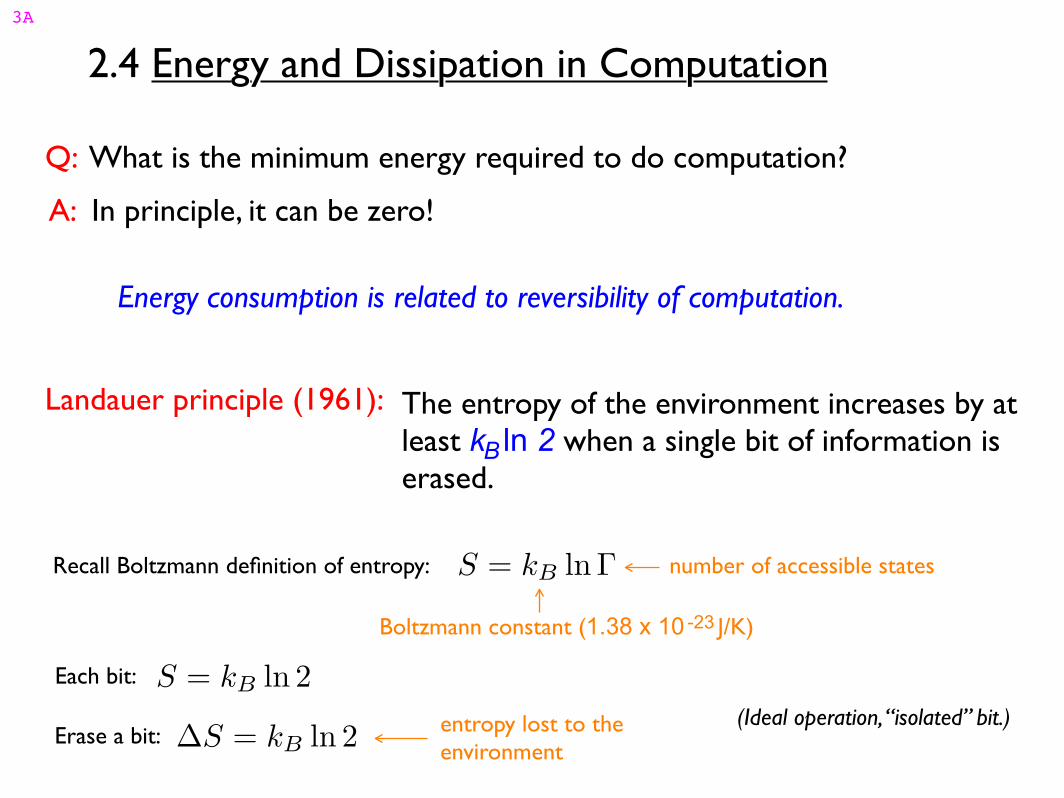
2.4 Energy and Dissipation in Computation
Q: What is the minimum energy required to do computation?
A: In principle, it can be zero!
Energy consumption is related to reversibility of computation.
Landauer principle (1961): The entropy of the environment increases by atleast k ln 2 when a single bit of information iserased.
B
Recall Boltzmann definition of entropy: S = kB lnΓ
Boltzmann constant (1.38 x 10 J/K)-23
number of accessible states
Each bit: S = kB ln 2
Erase a bit: ∆S = kB ln 2entropy lost to theenvironment
(Ideal operation, “isolated” bit.)
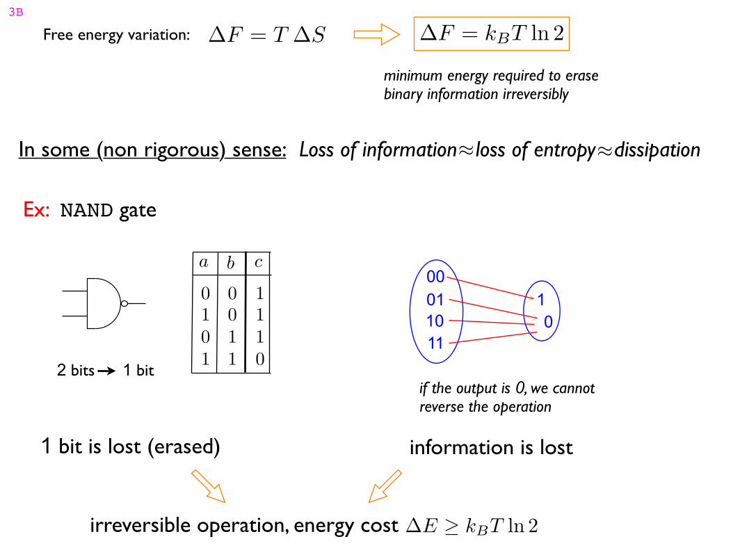
3B
Free energy variation: ∆F = T ∆S ∆F = kBT ln 2
minimum energy required to erasebinary information irreversibly
In some (non rigorous) sense: Loss of information loss of entropy dissipation ≈ ≈
Ex: NAND gate
0
1
a b c
0
0
0
1
1
1
1
0
1
1
00011011
01
if the output is 0, we cannotreverse the operation
2 bits 1 bit
1 bit is lost (erased) information is lost
irreversible operation, energy cost ∆E ≥ kBT ln 2
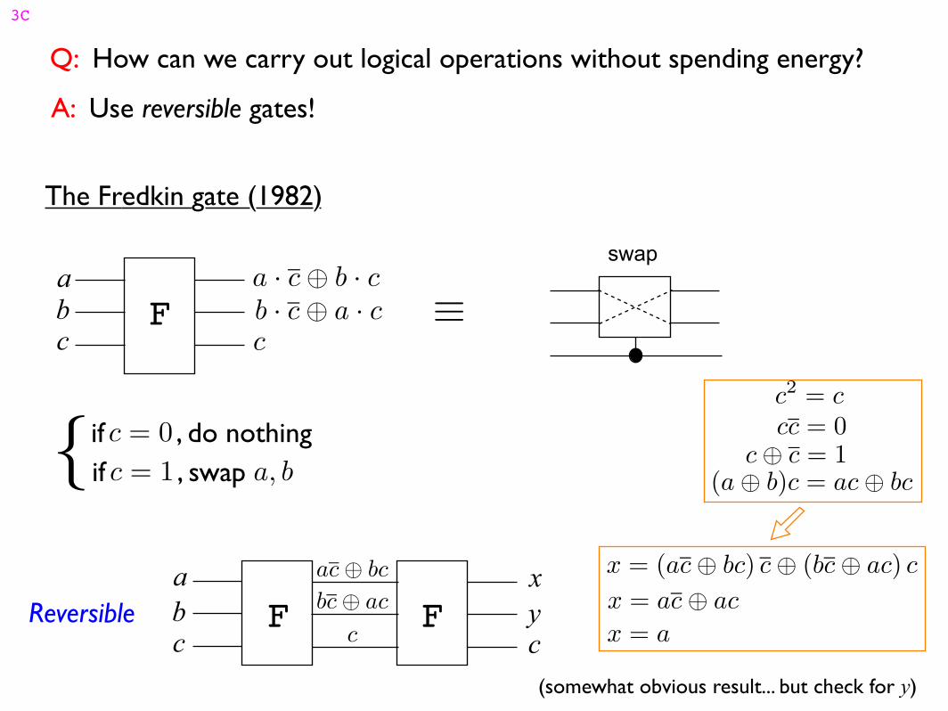
3C
Q: How can we carry out logical operations without spending energy?
A: Use reversible gates!
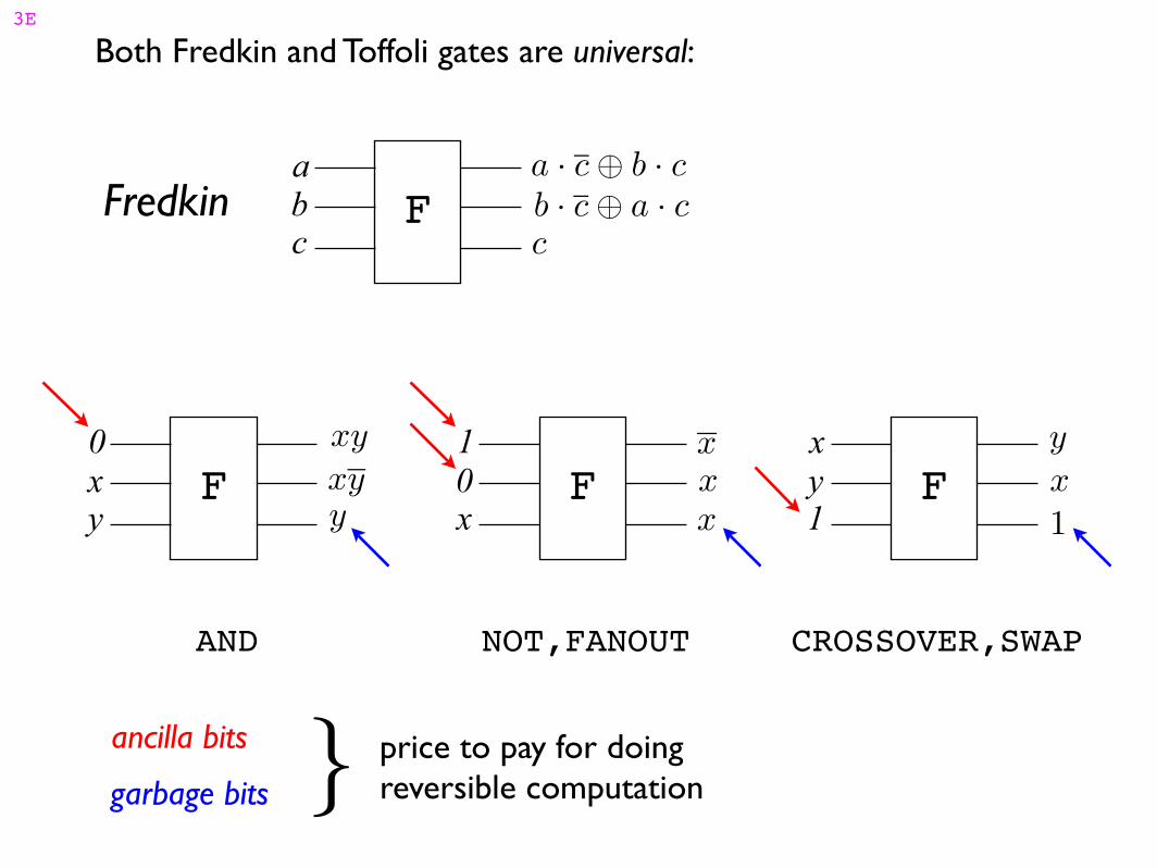
The Fredkin gate (1982)
Fabc
a · c ⊕ b · c
b · c ⊕ a · c
c
swap
≡
if , do nothingc = 0
if , swap c = 1 a, b{
abc
F Fxyc
bc ⊕ ac
ac ⊕ bc
c
Reversible
x = (ac ⊕ bc) c ⊕ (bc ⊕ ac) c
x = ac ⊕ ac
x = a
(somewhat obvious result... but check for y)
cc = 0
c ⊕ c = 1
(a ⊕ b)c = ac ⊕ bc
c2
= c
3D
c
x
c x
c
c x
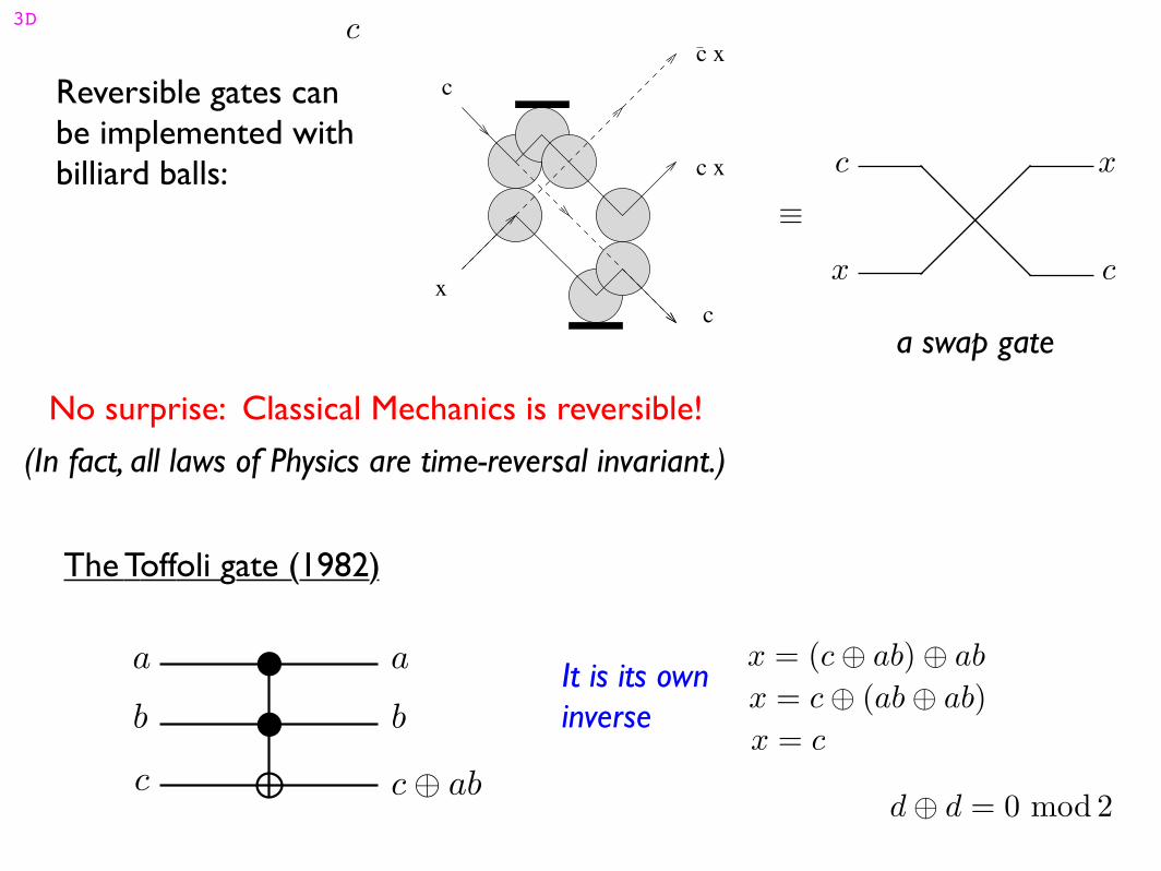
Reversible gates canbe implemented withbilliard balls:
c
c
x
x
c
a swap gate
≡
No surprise: Classical Mechanics is reversible!
(In fact, all laws of Physics are time-reversal invariant.)
The Toffoli gate (1982)
a
b
c c ⊕ ab
b
a
d ⊕ d = 0 mod 2
x = (c ⊕ ab) ⊕ ab
x = c ⊕ (ab ⊕ ab)x = c
It is its owninverse
3E
Both Fredkin and Toffoli gates are universal:
F0xy y
xy
xy F10x x
x
x
Fxy1
x
1
y
AND NOT,FANOUT CROSSOVER,SWAP
ancilla bits
garbage bits } price to pay for doingreversible computation
Fabc
a · c ⊕ b · c
b · c ⊕ a · c
c
Fredkin
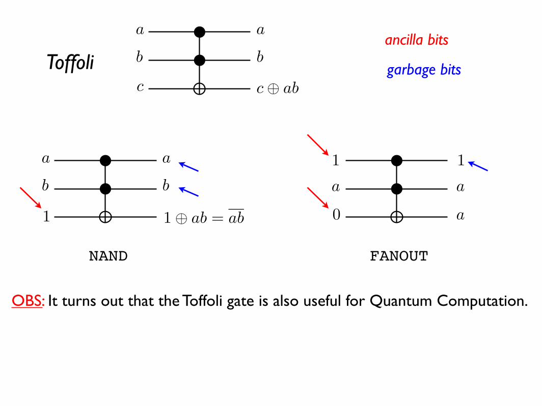
a
b
c c ⊕ ab
b
a
Toffoli
a
b b
a
1 1 ⊕ ab = ab
NAND FANOUT
ancilla bits
garbage bits
OBS: It turns out that the Toffoli gate is also useful for Quantum Computation.
a a
1
a
1
0
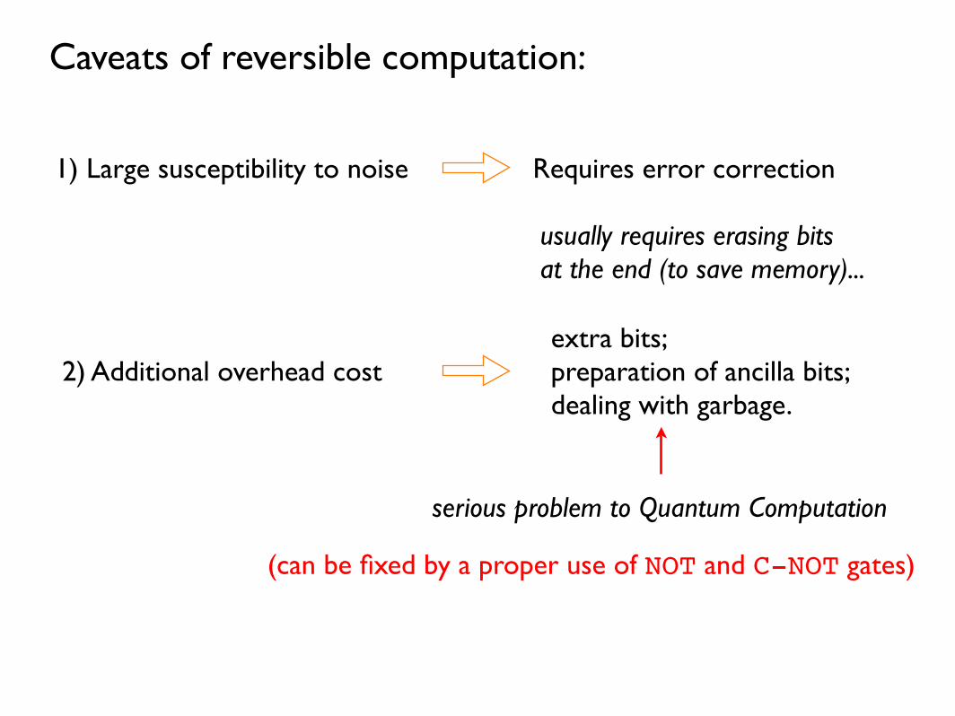
Caveats of reversible computation:
1) Large susceptibility to noise Requires error correction
usually requires erasing bitsat the end (to save memory)...
2) Additional overhead costextra bits; preparation of ancilla bits;dealing with garbage.
serious problem to Quantum Computation
(can be fixed by a proper use of NOT and C-NOT gates)