Introduction to Probability for Graphical Models

CSC 412 Kaustav Kundu

Thursday January 14, 2016

*Most slides based on Kevin Swersky’s slides, Inmar Givoni’s slides, Danny Tarlow’s slides, Jasper Snoek’s slides, Sam Roweis ‘s review of probability, Bishop’s book, and some images from Wikipedia

Outline

• Basics • Probability rules • Exponential family models • Maximum likelihood • Conjugate Bayesian inference (time

permitting)

Why Represent Uncertainty?

• The world is full of uncertainty – “What will the weather be like today?” – “Will I like this movie?” – “Is there a person in this image?”

• We’re trying to build systems that understand and (possibly) interact with the real world

• We often can’t prove something is true, but we can still ask how likely different outcomes are or ask for the most likely explanation

• Sometimes probability gives a concise description of an otherwise complex phenomenon.

Why Use Probability to Represent Uncertainty?

• Write down simple, reasonable criteria that you'd want from a system of uncertainty (common sense stuff), and you always get probability.

• Cox Axioms (Cox 1946); See Bishop, Section 1.2.3

• We will restrict ourselves to a relatively informal discussion of probability theory.

Notation• A random variable X represents outcomes or

states of the world. • We will write p(x) to mean Probability(X = x) • Sample space: the space of all possible

outcomes (may be discrete, continuous, or mixed)

• p(x) is the probability mass (density) function – Assigns a number to each point in sample space – Non-negative, sums (integrates) to 1 – Intuitively: how often does x occur, how much do

we believe in x.

Joint Probability Distribution• Prob(X=x, Y=y) – “Probability of X=x and Y=y” – p(x, y)

Conditional Probability Distribution

• Prob(X=x|Y=y) – “Probability of X=x given Y=y” – p(x|y) = p(x,y)/p(y)

The Rules of Probability

• Sum Rule (marginalization/summing out):

• Product/Chain Rule:

),...,,(...)(

),()(

2112 3

Nx x x

y

xxxpxp

yxpxp

N

∑∑ ∑

∑

=

=

),...,|()...|()(),...,()()|(),(

111211 −=

=

NNN xxxpxxpxpxxpxpxypyxp

Bayes’ Rule

• One of the most important formulas in probability theory

• This gives us a way of “reversing” conditional probabilities

∑==

')'()'|(

)()|()()()|()|(

x

xpxypxpxyp

ypxpxyp

yxp

Independence

• Two random variables are said to be independent iff their joint distribution factors

• Two random variables are conditionally independent given a third if they are independent after conditioning on the third

)()()()|()()|(),( ypxpypyxpxpxypyxp ===

zzxpzypzxpzxypzyxp ∀== )|()|()|(),|()|,(

Continuous Random Variables• Outcomes are real values. Probability

density functions define distributions. – E.g.,

• Continuous joint distributions: replace sums with integrals, and everything holds – E.g., Marginalization and conditional

probability

∫∫ ==yy

yPyzxPzyxPzxP )()|,(),,(),(

⎭⎬⎫

⎩⎨⎧ −−= 2

2 )(21

exp21

),|( µσσπ

σµ xxP

Summarizing Probability Distributions

• It is often useful to give summaries of distributions without defining the whole distribution (E.g., mean and variance)

• Mean: • Variance:

dxxpxxxEx

)(][ ∫ ⋅==

dxxpxExxx

)(])[()var( 2∫ ⋅−=

=E[x2 ]−E[x]2

Summarizing Probability Distributions

• It is often useful to give summaries of distributions without defining the whole distribution (E.g., mean and variance)

• Mean: • Variance:

dxxpxxxEx

)(][ ∫ ⋅==

dxxpxExxx

)(])[()var( 2∫ ⋅−=

=E[x2 ]−E[x]2

Exponential Family

• Family of probability distributions • Many of the standard distributions belong

to this family – Bernoulli, Binomial/Multinomial, Poisson,

Normal (Gaussian), Beta/Dirichlet,…

• Share many important properties – e.g. They have a conjugate prior (we’ll get to

that later. Important for Bayesian statistics)

Definition• The exponential family of distributions over x,

given parameter η (eta) is the set of distributions of the form

• x-scalar/vector, discrete/continuous • η – ‘natural parameters’ • u(x) – some function of x (sufficient statistic) • g(η) – normalizer

• h(x) – base measure (often constant)

)}(exp{)()()|( xugxhxp Tηηη =

1)}(exp{)()( =∫ dxxuxhg Tηη

Sufficient Statistics

• Vague definition: called so because they completely summarize a distribution.

• Less vague: they are the only part of the distribution that interacts with the parameters and are therefore sufficient to estimate the parameters.

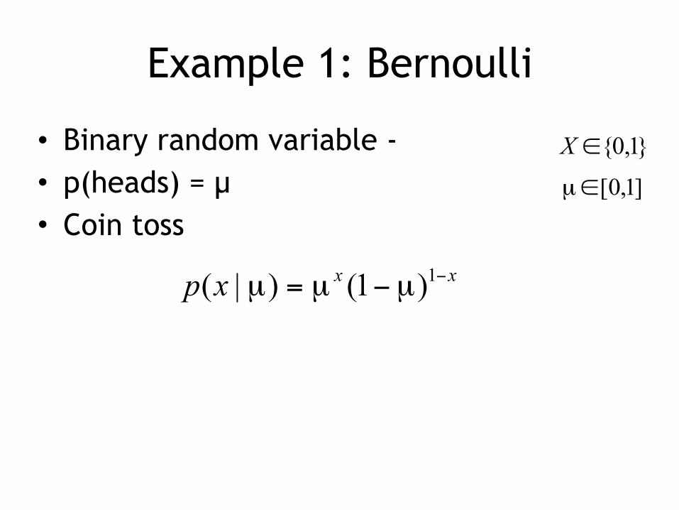
Example 1: Bernoulli

• Binary random variable - • p(heads) = µ • Coin toss

xxxp −−= 1)1()|( µµµ

}1,0{∈X]1,0[∈µ

Example 1: Bernoulli

xxxp −−= 1)1()|( µµµ

}1

exp{ln)1(

)}1ln()1(lnexp{

xu

xx

⎟⎠

⎞⎜⎝

⎛−

−=

−−+=

µµ

µµ

)()(11)(

1ln

)(1)(

ηση

ησµµ

µη

η

−=

+==⇒⎟⎟

⎠

⎞⎜⎜⎝

⎛

−=

=

=

−

ge

xxuxh

)}(exp{)()()|( xugxhxp Tηηη =

)exp()()|( xxp ηηση −=

Example 2: Multinomial• p(value k) = µk

• For a single observation – die toss – Sometimes called Categorical

• For multiple observations – integer counts on N trials – Prob(1 came out 3 times, 2 came out once,…,

6 came out 7 times if I tossed a die 20 times)

1],1,0[1

=∈ ∑=

M

kkk µµ

∏∏ =

=M

k

xk

kk

Mk

xN

xxP1

1 !!)|,...,( µµ

∑=

=M

kk Nx

1

Example 2: Multinomial (1 observation)

}lnexp{1∑=

=M

kkkx µ

xxx=

=

)(1)(

uh

)}(exp{)()()|( xugxhxp Tηηη =

∏=

=M

k

xkMkxxP

11 )|,...,( µµ

)exp()|( xx Tp ηη =

Parameters are not independent due to constraint of summing to 1, there’s a slightly more involved notation to address that, see Bishop 2.4

Example 3: Normal (Gaussian) Distribution

• Gaussian (Normal)

⎭⎬⎫

⎩⎨⎧ −−= 2

2 )(21

exp21

),|( µσσπ

σµ xxp

Example 3: Normal (Gaussian) Distribution

• µ is the mean • σ2 is the variance • Can verify these by computing integrals.

E.g.,

⎭⎬⎫

⎩⎨⎧ −−= 2

2 )(21

exp21

),|( µσσπ

σµ xxp

€

x ⋅ 12πσ

exp −12σ 2 (x −µ)2

⎧ ⎨ ⎩

⎫ ⎬ ⎭ dx = µ

x→−∞

x→∞

∫

Example 3: Normal (Gaussian) Distribution

• Multivariate Gaussian

€

P(x |µ,∑) = 2π ∑−1/ 2 exp −12(x −µ)T ∑−1(x −µ)

⎧ ⎨ ⎩

⎫ ⎬ ⎭

Example 3: Normal (Gaussian) Distribution

• Multivariate Gaussian

• x is now a vector • µ is the mean vector • Σ is the covariance matrix

⎭⎬⎫

⎩⎨⎧ −∑−−∑=∑ −− )()(21

exp2),|( 12/1µµπµ xxxp T

Important Properties of Gaussians

• All marginals of a Gaussian are again Gaussian

• Any conditional of a Gaussian is Gaussian • The product of two Gaussians is again

Gaussian • Even the sum of two independent Gaussian

RVs is a Gaussian. • Beyond the scope of this tutorial, but very

important: marginalization and conditioning rules for multivariate Gaussians.

Gaussian marginalization visualization

Exponential Family Representation

}21

exp{)4

exp()2()2(

}21

21

exp{21

)(21

exp21

),|(

2222

212

1

221

222

22

22

⎥⎦

⎤⎢⎣

⎡⎥⎦

⎤⎢⎣

⎡ −−=

=−

++−

=

⎭⎬⎫

⎩⎨⎧ −−=

−

xx

xx

xxp

σσ

µ

η

ηηπ

µσσ

µ

σσπ

µσσπ

σµ

)}(exp{)()()|( xugxhxp Tηηη =

)(xh )(ηg Tη )(xu

Example: Maximum Likelihood For a 1D Gaussian

• Suppose we are given a data set of samples of a Gaussian random variable X, D={x1,…, xN} and told that the variance of the data is σ2

What is our best guess of µ? *Need to assume data is independent and

identically distributed (i.i.d.)

x1 x2 xN…

Example: Maximum Likelihood For a 1D Gaussian

What is our best guess of µ? • We can write down the likelihood function:

• We want to choose the µ that maximizes this expression – Take log, then basic calculus: differentiate

w.r.t. µ, set derivative to 0, solve for µ to get sample mean

∏ ∏= = ⎭

⎬⎫

⎩⎨⎧ −−==µ

N

i

N

i

ii xxpdp1 1

22 )(

21

exp21

),|()|( µσσπ

σµ

€

µML =1N

xii=1

N∑

Example: Maximum Likelihood For a 1D Gaussian

x1 x2 xN…µML

σML

Maximum Likelihood

ML estimation of model parameters for Exponential Family

p(D |η) = p(x1,..., xN ) = h(xn)∏( )g(η)N exp{ηT u(xnn∑ )}

∂ln(p(D |η))

∂η= ..., set to 0, solve for ∇g(η)

∑=

=∇−N

nnML xu

Ng

1)(1)(ln η

• Can in principle be solved to get estimate for eta. • The solution for the ML estimator depends on the data only through sum over u, which is therefore called sufficient statistic • What we need to store in order to estimate parameters.

• is the likelihood function • is the prior probability of (or our prior

belief over) θ – our beliefs over what models are likely or not

before seeing any data • is the

normalization constant or partition function

• is the posterior distribution – Readjustment of our prior beliefs in the face of

data

Bayesian Probabilities

)()()|()|(

dppdpdp θθ

θ =

∫= θθθ dPdpdp )()|()(

)|( θdp)(θp

)|( dp θ

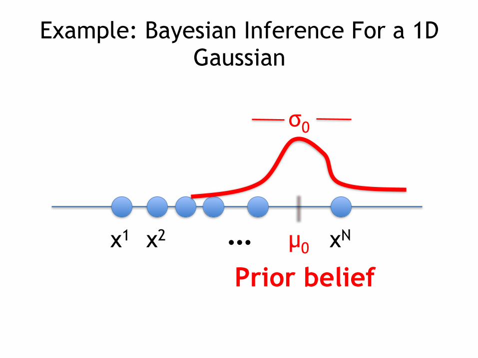
Example: Bayesian Inference For a 1D Gaussian

• Suppose we have a prior belief that the mean of some random variable X is µ0 and the variance of our belief is σ0

2

• We are then given a data set of samples of X, d={x1,…, xN} and somehow know that the variance of the data is σ2

What is the posterior distribution over (our belief about the value of) µ?

Example: Bayesian Inference For a 1D Gaussian

x1 x2 xN…

Example: Bayesian Inference For a 1D Gaussian

x1 x2 xN… µ0

σ0

Prior belief

Example: Bayesian Inference For a 1D Gaussian

• Remember from earlier • is the likelihood function

• is the prior probability of (or our prior belief over) µ

)()()|()|(

dppdpdp µµ

=µ

)|( µdp

∏ ∏= = ⎭

⎬⎫

⎩⎨⎧ −−==µ

N

i

N

i

ii xxPdp1 1

22 )(

21

exp21

),|()|( µσσπ

σµ

)(µp

⎭⎬⎫

⎩⎨⎧

µ−µ−=µµ 202

0000 )(

21

exp21

),|(σσπ

σp

Example: Bayesian Inference For a 1D Gaussian

),|()|()()|()|(

NNDppDpDp

σµµ=µ

µµ∝µ

Normal

€

µN =σ 2

Nσ 02 +σ 2 µ0 +

Nσ 02

Nσ 02 +σ 2 µML

1σN2 =

1σ 02 +

Nσ 2

where

Example: Bayesian Inference For a 1D Gaussian

x1 x2 xN… µ0

σ0

Prior belief

Example: Bayesian Inference For a 1D Gaussian

x1 x2 xN… µ0

σ0

Prior beliefµML

σML

Maximum Likelihood

Example: Bayesian Inference For a 1D Gaussian

x1 x2 xNµN

σN

Prior beliefMaximum Likelihood

Posterior Distribution

Conjugate Priors• Notice in the Gaussian parameter estimation

example that the functional form of the posterior was that of the prior (Gaussian)

• Priors that lead to that form are called ‘conjugate priors’

• For any member of the exponential family there exists a conjugate prior that can be written like

• Multiply by likelihood to obtain posterior (up to normalization) of the form

• Notice the addition to the sufficient statistic • ν is the effective number of pseudo-

observations.

}exp{)(),(),|( χνηηνχνχη ν Tgfp =

)})((exp{)(),,|(1

νχηηνχη ν +∝ ∑=

+N

nn

TN xugDp

Conjugate Priors - Examples

• Beta for Bernoulli/binomial • Dirichlet for categorical/multinomial • Normal for Normal