Introduction to Probability and Statistics Using R!
386
Introduction to Probability and Statistics Using R G. Jay Kerns First Edition
-
Upload
dmytro-shteflyuk -
Category
Documents
-
view
3.217 -
download
9
description
This is a textbook for an undergraduate course in probability and statistics. The approximate prerequisites are two or three semesters of calculus and some linear algebra. Students attending the class include mathematics, engineering, and computer science majors...
Transcript of Introduction to Probability and Statistics Using R!
Introduction to Probabilityand Statistics Using R
G. Jay Kerns
First Edition

ii
IPSUR: Introduction to Probability and Statistics Using RCopyright© 2010 G. Jay KernsISBN: 978-0-557-24979-4
Permission is granted to copy, distribute and/or modify this document under the terms of theGNU Free Documentation License, Version 1.3 or any later version published by the FreeSoftware Foundation; with no Invariant Sections, no Front-Cover Texts, and no Back-CoverTexts. A copy of the license is included in the section entitled “GNU Free DocumentationLicense”.
Date: July 28, 2010
Contents
Preface vii
List of Figures xiii
List of Tables xv
1 An Introduction to Probability and Statistics 1
1.1 Probability . . . . . . . . . . . . . . . . . . . . . . . . . . . . . . . . . . . . . 11.2 Statistics . . . . . . . . . . . . . . . . . . . . . . . . . . . . . . . . . . . . . . 1Chapter Exercises . . . . . . . . . . . . . . . . . . . . . . . . . . . . . . . . . . . . 3
2 An Introduction to R 5
2.1 Downloading and Installing R . . . . . . . . . . . . . . . . . . . . . . . . . . 52.2 Communicating with R . . . . . . . . . . . . . . . . . . . . . . . . . . . . . . 62.3 Basic R Operations and Concepts . . . . . . . . . . . . . . . . . . . . . . . . . 82.4 Getting Help . . . . . . . . . . . . . . . . . . . . . . . . . . . . . . . . . . . . 142.5 External Resources . . . . . . . . . . . . . . . . . . . . . . . . . . . . . . . . 152.6 Other Tips . . . . . . . . . . . . . . . . . . . . . . . . . . . . . . . . . . . . . 16Chapter Exercises . . . . . . . . . . . . . . . . . . . . . . . . . . . . . . . . . . . . 17
3 Data Description 19
3.1 Types of Data . . . . . . . . . . . . . . . . . . . . . . . . . . . . . . . . . . . 193.2 Features of Data Distributions . . . . . . . . . . . . . . . . . . . . . . . . . . 333.3 Descriptive Statistics . . . . . . . . . . . . . . . . . . . . . . . . . . . . . . . 353.4 Exploratory Data Analysis . . . . . . . . . . . . . . . . . . . . . . . . . . . . 403.5 Multivariate Data and Data Frames . . . . . . . . . . . . . . . . . . . . . . . . 453.6 Comparing Populations . . . . . . . . . . . . . . . . . . . . . . . . . . . . . . 47Chapter Exercises . . . . . . . . . . . . . . . . . . . . . . . . . . . . . . . . . . . . 53
4 Probability 65
4.1 Sample Spaces . . . . . . . . . . . . . . . . . . . . . . . . . . . . . . . . . . . 654.2 Events . . . . . . . . . . . . . . . . . . . . . . . . . . . . . . . . . . . . . . . 704.3 Model Assignment . . . . . . . . . . . . . . . . . . . . . . . . . . . . . . . . 754.4 Properties of Probability . . . . . . . . . . . . . . . . . . . . . . . . . . . . . 804.5 Counting Methods . . . . . . . . . . . . . . . . . . . . . . . . . . . . . . . . . 844.6 Conditional Probability . . . . . . . . . . . . . . . . . . . . . . . . . . . . . . 894.7 Independent Events . . . . . . . . . . . . . . . . . . . . . . . . . . . . . . . . 954.8 Bayes’ Rule . . . . . . . . . . . . . . . . . . . . . . . . . . . . . . . . . . . . 984.9 Random Variables . . . . . . . . . . . . . . . . . . . . . . . . . . . . . . . . . 102Chapter Exercises . . . . . . . . . . . . . . . . . . . . . . . . . . . . . . . . . . . . 105
iii
iv CONTENTS
5 Discrete Distributions 107
5.1 Discrete Random Variables . . . . . . . . . . . . . . . . . . . . . . . . . . . . 1075.2 The Discrete Uniform Distribution . . . . . . . . . . . . . . . . . . . . . . . . 1105.3 The Binomial Distribution . . . . . . . . . . . . . . . . . . . . . . . . . . . . 1115.4 Expectation and Moment Generating Functions . . . . . . . . . . . . . . . . . 1165.5 The Empirical Distribution . . . . . . . . . . . . . . . . . . . . . . . . . . . . 1205.6 Other Discrete Distributions . . . . . . . . . . . . . . . . . . . . . . . . . . . 1235.7 Functions of Discrete Random Variables . . . . . . . . . . . . . . . . . . . . . 130Chapter Exercises . . . . . . . . . . . . . . . . . . . . . . . . . . . . . . . . . . . . 132
6 Continuous Distributions 137
6.1 Continuous Random Variables . . . . . . . . . . . . . . . . . . . . . . . . . . 1376.2 The Continuous Uniform Distribution . . . . . . . . . . . . . . . . . . . . . . 1426.3 The Normal Distribution . . . . . . . . . . . . . . . . . . . . . . . . . . . . . 1436.4 Functions of Continuous Random Variables . . . . . . . . . . . . . . . . . . . 1466.5 Other Continuous Distributions . . . . . . . . . . . . . . . . . . . . . . . . . . 150Chapter Exercises . . . . . . . . . . . . . . . . . . . . . . . . . . . . . . . . . . . . 155
7 Multivariate Distributions 157
7.1 Joint and Marginal Probability Distributions . . . . . . . . . . . . . . . . . . . 1577.2 Joint and Marginal Expectation . . . . . . . . . . . . . . . . . . . . . . . . . . 1637.3 Conditional Distributions . . . . . . . . . . . . . . . . . . . . . . . . . . . . . 1657.4 Independent Random Variables . . . . . . . . . . . . . . . . . . . . . . . . . . 1677.5 Exchangeable Random Variables . . . . . . . . . . . . . . . . . . . . . . . . . 1707.6 The Bivariate Normal Distribution . . . . . . . . . . . . . . . . . . . . . . . . 1707.7 Bivariate Transformations of Random Variables . . . . . . . . . . . . . . . . . 1727.8 Remarks for the Multivariate Case . . . . . . . . . . . . . . . . . . . . . . . . 1757.9 The Multinomial Distribution . . . . . . . . . . . . . . . . . . . . . . . . . . . 178Chapter Exercises . . . . . . . . . . . . . . . . . . . . . . . . . . . . . . . . . . . . 180
8 Sampling Distributions 181
8.1 Simple Random Samples . . . . . . . . . . . . . . . . . . . . . . . . . . . . . 1828.2 Sampling from a Normal Distribution . . . . . . . . . . . . . . . . . . . . . . 1828.3 The Central Limit Theorem . . . . . . . . . . . . . . . . . . . . . . . . . . . . 1858.4 Sampling Distributions of Two-Sample Statistics . . . . . . . . . . . . . . . . 1878.5 Simulated Sampling Distributions . . . . . . . . . . . . . . . . . . . . . . . . 189Chapter Exercises . . . . . . . . . . . . . . . . . . . . . . . . . . . . . . . . . . . . 191
9 Estimation 193
9.1 Point Estimation . . . . . . . . . . . . . . . . . . . . . . . . . . . . . . . . . . 1939.2 Confidence Intervals for Means . . . . . . . . . . . . . . . . . . . . . . . . . . 2029.3 Confidence Intervals for Di!erences of Means . . . . . . . . . . . . . . . . . . 2089.4 Confidence Intervals for Proportions . . . . . . . . . . . . . . . . . . . . . . . 2109.5 Confidence Intervals for Variances . . . . . . . . . . . . . . . . . . . . . . . . 2129.6 Fitting Distributions . . . . . . . . . . . . . . . . . . . . . . . . . . . . . . . . 2129.7 Sample Size and Margin of Error . . . . . . . . . . . . . . . . . . . . . . . . . 2129.8 Other Topics . . . . . . . . . . . . . . . . . . . . . . . . . . . . . . . . . . . . 214Chapter Exercises . . . . . . . . . . . . . . . . . . . . . . . . . . . . . . . . . . . . 215
CONTENTS v
10 Hypothesis Testing 217
10.1 Introduction . . . . . . . . . . . . . . . . . . . . . . . . . . . . . . . . . . . . 21710.2 Tests for Proportions . . . . . . . . . . . . . . . . . . . . . . . . . . . . . . . 21810.3 One Sample Tests for Means and Variances . . . . . . . . . . . . . . . . . . . 22410.4 Two-Sample Tests for Means and Variances . . . . . . . . . . . . . . . . . . . 22710.5 Other Hypothesis Tests . . . . . . . . . . . . . . . . . . . . . . . . . . . . . . 22810.6 Analysis of Variance . . . . . . . . . . . . . . . . . . . . . . . . . . . . . . . 22910.7 Sample Size and Power . . . . . . . . . . . . . . . . . . . . . . . . . . . . . . 230Chapter Exercises . . . . . . . . . . . . . . . . . . . . . . . . . . . . . . . . . . . . 232
11 Simple Linear Regression 235
11.1 Basic Philosophy . . . . . . . . . . . . . . . . . . . . . . . . . . . . . . . . . 23511.2 Estimation . . . . . . . . . . . . . . . . . . . . . . . . . . . . . . . . . . . . . 23911.3 Model Utility and Inference . . . . . . . . . . . . . . . . . . . . . . . . . . . . 24811.4 Residual Analysis . . . . . . . . . . . . . . . . . . . . . . . . . . . . . . . . . 25211.5 Other Diagnostic Tools . . . . . . . . . . . . . . . . . . . . . . . . . . . . . . 259Chapter Exercises . . . . . . . . . . . . . . . . . . . . . . . . . . . . . . . . . . . . 266
12 Multiple Linear Regression 267
12.1 The Multiple Linear Regression Model . . . . . . . . . . . . . . . . . . . . . . 26712.2 Estimation and Prediction . . . . . . . . . . . . . . . . . . . . . . . . . . . . . 27012.3 Model Utility and Inference . . . . . . . . . . . . . . . . . . . . . . . . . . . . 27712.4 Polynomial Regression . . . . . . . . . . . . . . . . . . . . . . . . . . . . . . 28012.5 Interaction . . . . . . . . . . . . . . . . . . . . . . . . . . . . . . . . . . . . . 28312.6 Qualitative Explanatory Variables . . . . . . . . . . . . . . . . . . . . . . . . . 28612.7 Partial F Statistic . . . . . . . . . . . . . . . . . . . . . . . . . . . . . . . . . 28912.8 Residual Analysis and Diagnostic Tools . . . . . . . . . . . . . . . . . . . . . 29112.9 Additional Topics . . . . . . . . . . . . . . . . . . . . . . . . . . . . . . . . . 292Chapter Exercises . . . . . . . . . . . . . . . . . . . . . . . . . . . . . . . . . . . . 296
13 Resampling Methods 297
13.1 Introduction . . . . . . . . . . . . . . . . . . . . . . . . . . . . . . . . . . . . 29713.2 Bootstrap Standard Errors . . . . . . . . . . . . . . . . . . . . . . . . . . . . . 29913.3 Bootstrap Confidence Intervals . . . . . . . . . . . . . . . . . . . . . . . . . . 30313.4 Resampling in Hypothesis Tests . . . . . . . . . . . . . . . . . . . . . . . . . 305Chapter Exercises . . . . . . . . . . . . . . . . . . . . . . . . . . . . . . . . . . . . 309
14 Categorical Data Analysis 311
15 Nonparametric Statistics 313
16 Time Series 315
A R Session Information 317
B GNU Free Documentation License 319
C History 327
D Data 329

vi CONTENTS
D.1 Data Structures . . . . . . . . . . . . . . . . . . . . . . . . . . . . . . . . . . 329D.2 Importing Data . . . . . . . . . . . . . . . . . . . . . . . . . . . . . . . . . . 334D.3 Creating New Data Sets . . . . . . . . . . . . . . . . . . . . . . . . . . . . . . 335D.4 Editing Data . . . . . . . . . . . . . . . . . . . . . . . . . . . . . . . . . . . . 335D.5 Exporting Data . . . . . . . . . . . . . . . . . . . . . . . . . . . . . . . . . . 336D.6 Reshaping Data . . . . . . . . . . . . . . . . . . . . . . . . . . . . . . . . . . 337
E Mathematical Machinery 339
E.1 Set Algebra . . . . . . . . . . . . . . . . . . . . . . . . . . . . . . . . . . . . 339E.2 Di!erential and Integral Calculus . . . . . . . . . . . . . . . . . . . . . . . . . 340E.3 Sequences and Series . . . . . . . . . . . . . . . . . . . . . . . . . . . . . . . 343E.4 The Gamma Function . . . . . . . . . . . . . . . . . . . . . . . . . . . . . . . 345E.5 Linear Algebra . . . . . . . . . . . . . . . . . . . . . . . . . . . . . . . . . . 345E.6 Multivariable Calculus . . . . . . . . . . . . . . . . . . . . . . . . . . . . . . 347
F Writing Reports with R 349F.1 What to Write . . . . . . . . . . . . . . . . . . . . . . . . . . . . . . . . . . . 349F.2 How to Write It with R . . . . . . . . . . . . . . . . . . . . . . . . . . . . . . 350F.3 Formatting Tables . . . . . . . . . . . . . . . . . . . . . . . . . . . . . . . . . 353F.4 Other Formats . . . . . . . . . . . . . . . . . . . . . . . . . . . . . . . . . . . 353
G Instructions for Instructors 355G.1 Generating This Document . . . . . . . . . . . . . . . . . . . . . . . . . . . . 356G.2 How to Use This Document . . . . . . . . . . . . . . . . . . . . . . . . . . . . 356G.3 Ancillary Materials . . . . . . . . . . . . . . . . . . . . . . . . . . . . . . . . 357G.4 Modifying This Document . . . . . . . . . . . . . . . . . . . . . . . . . . . . 357
H RcmdrTestDrive Story 359
Bibliography 363
Index 369
Preface
This book was expanded from lecture materials I use in a one semester upper-division under-graduate course entitled Probability and Statistics at Youngstown State University. Those lec-ture materials, in turn, were based on notes that I transcribed as a graduate student at BowlingGreen State University. The course for which the materials were written is 50-50 Probabil-ity and Statistics, and the attendees include mathematics, engineering, and computer sciencemajors (among others). The catalog prerequisites for the course are a full year of calculus.
The book can be subdivided into three basic parts. The first part includes the introductionsand elementary descriptive statistics; I want the students to be knee-deep in data right out ofthe gate. The second part is the study of probability, which begins at the basics of sets andthe equally likely model, journeys past discrete/continuous random variables, and continuesthrough to multivariate distributions. The chapter on sampling distributions paves the way tothe third part, which is inferential statistics. This last part includes point and interval estimation,hypothesis testing, and finishes with introductions to selected topics in applied statistics.
I usually only have time in one semester to cover a small subset of this book. I cover thematerial in Chapter 2 in a class period that is supplemented by a take-home assignment forthe students. I spend a lot of time on Data Description, Probability, Discrete, and ContinuousDistributions. I mention selected facts from Multivariate Distributions in passing, and discussthe meaty parts of Sampling Distributions before moving right along to Estimation (which isanother chapter I dwell on considerably). Hypothesis Testing goes faster after all of the previouswork, and by that time the end of the semester is in sight. I normally choose one or two finalchapters (sometimes three) from the remaining to survey, and regret at the end that I did nothave the chance to cover more.
In an attempt to be correct I have included material in this book which I would normally notmention during the course of a standard lecture. For instance, I normally do not highlight theintricacies of measure theory or integrability conditionswhen speaking to the class. Moreover, Ioften stray from the matrix approach to multiple linear regression because many of my studentshave not yet been formally trained in linear algebra. That being said, it is important to me forthe students to hold something in their hands which acknowledges the world of mathematicsand statistics beyond the classroom, and which may be useful to them for many semesters tocome. It also mirrors my own experience as a student.
The vision for this document is a more or less self contained, essentially complete, correct,introductory textbook. There should be plenty of exercises for the student, with full solutionsfor some, and no solutions for others (so that the instructor may assign them for grading).By Sweave’s dynamic nature it is possible to write randomly generated exercises and I hadplanned to implement this idea already throughout the book. Alas, there are only 24 hours in aday. Look for more in future editions.
Seasoned readers will be able to detect my origins: Probability and Statistical Inference
by Hogg and Tanis [44], Statistical Inference by Casella and Berger [13], and Theory of Point
Estimation/Testing Statistical Hypotheses by Lehmann [59, 58]. I highly recommend each of
vii
viii CONTENTS
those books to every reader of this one. Some R books with “introductory” in the title that Irecommend are Introductory Statistics with R by Dalgaard [19] and Using R for Introductory
Statistics by Verzani [87]. Surely there are many, many other good introductory books aboutR, but frankly, I have tried to steer clear of them for the past year or so to avoid any undueinfluence on my own writing.
I would like to make special mention of two other books: Introduction to Statistical Thoughtby Michael Lavine [56] and Introduction to Probability by Grinstead and Snell [37]. Both ofthese books are free and are what ultimately convinced me to release IPSUR under a free license,too.
Please bear in mind that the title of this book is “Introduction to Probability and StatisticsUsing R”, and not “Introduction to R Using Probability and Statistics”, nor even “Introductionto Probability and Statistics and R Using Words”. The people at the party are Probabilityand Statistics; the handshake is R. There are several important topics about R which someindividuals will feel are underdeveloped, glossed over, or wantonly omitted. Some will feel thesame way about the probabilistic and/or statistical content. Still others will just want to learn Rand skip all of the mathematics.
Despite any misgivings: here it is, warts and all. I humbly invite said individuals to takethis book, with the GNU Free Documentation License (GNU-FDL) in hand, and make it better.In that spirit there are at least a few ways in my view in which this book could be improved.
Better data. The data analyzed in this book are almost entirely from the datasets packagein base R, and here is why:
1. I made a conscious e!ort to minimize dependence on contributed packages,
2. The data are instantly available, already in the correct format, so we need not taketime to manage them, and
3. The data are real.
I made no attempt to choose data sets that would be interesting to the students; rather,data were chosen for their potential to convey a statistical point. Many of the data setsare decades old or more (for instance, the data used to introduce simple linear regressionare the speeds and stopping distances of cars in the 1920’s).
In a perfect world with infinite time I would research and contribute recent, real data in acontext crafted to engage the students in every example. One day I hope to stumble oversaid time. In the meantime, I will add new data sets incrementally as time permits.
More proofs. I would like to include more proofs for the sake of completeness (I understandthat some people would not consider more proofs to be improvement). Many proofshave been skipped entirely, and I am not aware of any rhyme or reason to the currentomissions. I will add more when I get a chance.
More and better graphics: I have not used the ggplot2 package [90] because I do not knowhow to use it yet. It is on my to-do list.
More and better exercises: There are only a few exercises in the first edition simply becauseI have not had time to write more. I have toyed with the exams package [38] and I believethat it is a right way to move forward. As I learn more about what the package can do Iwould like to incorporate it into later editions of this book.
CONTENTS ix
About This Document
IPSUR contains many interrelated parts: theDocument, the Program, the Package, and the An-cillaries. In short, the Document is what you are reading right now. The Program provides ane"cient means to modify the Document. The Package is an R package that houses the Programand the Document. Finally, the Ancillaries are extra materials that reside in the Package andwere produced by the Program to supplement use of the Document. We briefly describe eachof them in turn.
The Document
The Document is that which you are reading right now – IPSUR’s raison d’être. There aretransparent copies (nonproprietary text files) and opaque copies (everything else). See theGNU-FDL in Appendix B for more precise language and details.
IPSUR.tex is a transparent copy of the Document to be typeset with a LATEX distribution suchas MikTEX or TEX Live. Any reader is free to modify the Document and release themodified version in accordance with the provisions of the GNU-FDL. Note that this filecannot be used to generate a randomized copy of the Document. Indeed, in its releasedform it is only capable of typesetting the exact version of IPSUR which you are currentlyreading. Furthermore, the .tex file is unable to generate any of the ancillary materials.
IPSUR-xxx.eps, IPSUR-xxx.pdf are the image files for every graph in the Document. Theseare needed when typesetting with LATEX.
IPSUR.pdf is an opaque copy of the Document. This is the file that instructors would likelywant to distribute to students.
IPSUR.dvi is another opaque copy of the Document in a di!erent file format.
The Program
The Program includes IPSUR.lyx and its nephew IPSUR.Rnw; the purpose of each is to giveindividuals a way to quickly customize the Document for their particular purpose(s).
IPSUR.lyx is the source LYX file for the Program, released under the GNU General PublicLicense (GNU GPL) Version 3. This file is opened, modified, and compiled with LYX, asophisticated open-source document processor, and may be used (together with Sweave)to generate a randomized, modified copy of the Document with brand new data sets forsome of the exercises and the solution manuals (in the Second Edition). Additionally,LYX can easily activate/deactivate entire blocks of the document, e.g. the proofs of thetheorems, the student solutions to the exercises, or the instructor answers to the prob-lems, so that the new author may choose which sections (s)he would like to include in thefinal Document (again, Second Edition). The IPSUR.lyx file is all that a person needs(in addition to a properly configured system – see Appendix G) to generate/compile/ex-port to all of the other formats described above and below, which includes the ancillarymaterials IPSUR.Rdata and IPSUR.R.
IPSUR.Rnw is another form of the source code for the Program, also released under the GNUGPL Version 3. It was produced by exporting IPSUR.lyx into R/Sweave format (.Rnw).

x CONTENTS
This file may be processed with Sweave to generate a randomized copy of IPSUR.tex – atransparent copy of the Document – together with the ancillary materials IPSUR.Rdataand IPSUR.R. Please note, however, that IPSUR.Rnw is just a simple text file whichdoes not support many of the extra features that LYX o!ers such as WYSIWYM editing,instantly (de)activating branches of the manuscript, and more.
The Package
There is a contributed package on CRAN, called IPSUR. The package a!ords many advantages,one being that it houses the Document in an easy-to-access medium. Indeed, a student can havethe Document at his/her fingertips with only three commands:
> install.packages("IPSUR")
> library(IPSUR)
> read(IPSUR)
Another advantage goes hand in hand with the Program’s license; since IPSUR is free, thesource code must be freely available to anyone that wants it. A package hosted on CRAN allowsthe author to obey the license by default.
A much more important advantage is that the excellent facilities at R-Forge are buildingand checking the package daily against patched and development versions of the absolute latestpre-release of R. If any problems surface then I will know about it within 24 hours.
And finally, suppose there is some sort of problem. The package structure makes it in-credibly easy for me to distribute bug-fixes and corrected typographical errors. As an author Ican make my corrections, upload them to the repository at R-Forge, and they will be reflectedworldwide within hours. We aren’t in Kansas anymore, Dorothy.
Ancillary Materials
These are extra materials that accompany IPSUR. They reside in the /etc subdirectory of thepackage source.
IPSUR.RData is a saved image of the R workspace at the completion of the Sweave processingof IPSUR. It can be loaded into memory with File ! Load Workspace or with the com-mand load("/path/to/IPSUR.Rdata"). Either method will make every single objectin the file immediately available and in memory. In particular, the data BLANK fromExercise BLANK in Chapter BLANK on page BLANK will be loaded. Type BLANK atthe command line (after loading IPSUR.RData) to see for yourself.
IPSUR.R is the exported R code from IPSUR.Rnw. With this script, literally every R commandfrom the entirety of IPSUR can be resubmitted at the command line.
Notation
We use the notation x or stem.leaf notation to denote objects, functions, etc.. The sequence“Statistics ! Summaries ! Active Dataset” means to click the Statistics menu item, next clickthe Summaries submenu item, and finally click Active Dataset.

CONTENTS xi
Acknowledgements
This book would not have been possible without the firm mathematical and statistical foun-dation provided by the professors at Bowling Green State University, including Drs. GáborSzékely, Craig Zirbel, Arjun K. Gupta, Hanfeng Chen, Truc Nguyen, and James Albert. Iwould also like to thank Drs. Neal Carothers and Kit Chan.
I would also like to thank my colleagues at Youngstown State University for their support.In particular, I would like to thank Dr. G. Andy Chang for showing me what it means to be astatistician.
I would like to thank Richard Heiberger for his insightful comments and improvements toseveral points and displays in the manuscript.
Finally, and most importantly, I would like to thank my wife for her patience and under-standing while I worked hours, days, months, and years on a free book. In retrospect, I can’tbelieve I ever got away with it.

xii CONTENTS
List of Figures
3.1.1 Strip charts of the precip, rivers, and discoveries data . . . . . . . . . 223.1.2 (Relative) frequency histograms of the precip data . . . . . . . . . . . . . 233.1.3 More histograms of the precip data . . . . . . . . . . . . . . . . . . . . . 243.1.4 Index plots of the LakeHuron data . . . . . . . . . . . . . . . . . . . . . . 273.1.5 Bar graphs of the state.region data . . . . . . . . . . . . . . . . . . . . 293.1.6 Pareto chart of the state.division data . . . . . . . . . . . . . . . . . . 313.1.7 Dot chart of the state.region data . . . . . . . . . . . . . . . . . . . . . 323.6.1 Boxplots of weight by feed type in the chickwts data . . . . . . . . . . . 503.6.2 Histograms of age by education level from the infert data . . . . . . . . 503.6.3 An xyplot of Petal.Length versus Petal.Width by Species in the
iris data . . . . . . . . . . . . . . . . . . . . . . . . . . . . . . . . . . . 513.6.4 A coplot of conc versus uptake by Type and Treatment in the CO2 data 52
4.5.1 The birthday problem . . . . . . . . . . . . . . . . . . . . . . . . . . . . . 89
5.3.1 Graph of the binom(size = 3, prob = 1/2) CDF . . . . . . . . . . . . . . 1155.3.2 The binom(size = 3, prob = 0.5) distribution from the distr package . . . 1165.5.1 The empirical CDF . . . . . . . . . . . . . . . . . . . . . . . . . . . . . . 122
6.5.1 Chi square distribution for various degrees of freedom . . . . . . . . . . . . 1526.5.2 Plot of the gamma(shape = 13, rate = 1) MGF . . . . . . . . . . . . . . 155
7.6.1 Graph of a bivariate normal PDF . . . . . . . . . . . . . . . . . . . . . . . 1737.9.1 Plot of a multinomial PMF . . . . . . . . . . . . . . . . . . . . . . . . . . 180
8.2.1 Student’s t distribution for various degrees of freedom . . . . . . . . . . . . 1858.5.1 Plot of simulated IQRs . . . . . . . . . . . . . . . . . . . . . . . . . . . . . 1908.5.2 Plot of simulated MADs . . . . . . . . . . . . . . . . . . . . . . . . . . . . 190
9.1.1 Capture-recapture experiment . . . . . . . . . . . . . . . . . . . . . . . . . 1959.1.2 Assorted likelihood functions for fishing, part two . . . . . . . . . . . . . . 1969.1.3 Species maximum likelihood . . . . . . . . . . . . . . . . . . . . . . . . . 1989.2.1 Simulated confidence intervals . . . . . . . . . . . . . . . . . . . . . . . . 2049.2.2 Confidence interval plot for the PlantGrowth data . . . . . . . . . . . . . . 206
10.2.1 Hypothesis test plot based on normal.and.t.dist from the HH package . . 22310.3.1 Hypothesis test plot based on normal.and.t.dist from the HH package . . 22610.6.1 Between group versus within group variation . . . . . . . . . . . . . . . . . 23110.6.2 Between group versus within group variation . . . . . . . . . . . . . . . . . 23210.6.3 Some F plots from the HH package . . . . . . . . . . . . . . . . . . . . . . 23310.7.1 Plot of significance level and power . . . . . . . . . . . . . . . . . . . . . . 234
xiii

xiv LIST OF FIGURES
11.1.1 Philosophical foundations of SLR . . . . . . . . . . . . . . . . . . . . . . . 23711.1.2 Scatterplot of dist versus speed for the cars data . . . . . . . . . . . . . 23811.2.1 Scatterplot with added regression line for the cars data . . . . . . . . . . . 24111.2.2 Scatterplot with confidence/prediction bands for the cars data . . . . . . . 24811.4.1 Normal q-q plot of the residuals for the cars data . . . . . . . . . . . . . . 25311.4.2 Plot of standardized residuals against the fitted values for the cars data . . . 25511.4.3 Plot of the residuals versus the fitted values for the cars data . . . . . . . . 25711.5.1 Cook’s distances for the cars data . . . . . . . . . . . . . . . . . . . . . . 26311.5.2 Diagnostic plots for the cars data . . . . . . . . . . . . . . . . . . . . . . . 265
12.1.1 Scatterplot matrix of trees data . . . . . . . . . . . . . . . . . . . . . . . 26912.1.2 3D scatterplot with regression plane for the trees data . . . . . . . . . . . 27012.4.1 Scatterplot of Volume versus Girth for the trees data . . . . . . . . . . . 28012.4.2 A quadratic model for the trees data . . . . . . . . . . . . . . . . . . . . . 28212.6.1 A dummy variable model for the trees data . . . . . . . . . . . . . . . . . 288
13.2.1 Bootstrapping the standard error of the mean, simulated data . . . . . . . . 30013.2.2 Bootstrapping the standard error of the median for the rivers data . . . . . 302

List of Tables
4.1 Sampling k from n objects with urnsamples . . . . . . . . . . . . . . . . . . 864.2 Rolling two dice . . . . . . . . . . . . . . . . . . . . . . . . . . . . . . . . . . 90
5.1 Correspondence between stats and distr . . . . . . . . . . . . . . . . . . . 116
7.1 Maximum U and sum V of a pair of dice rolls (X, Y) . . . . . . . . . . . . . . . 1607.2 Joint values of U = max(X, Y) and V = X + Y . . . . . . . . . . . . . . . . . . 1607.3 The joint PMF of (U,V) . . . . . . . . . . . . . . . . . . . . . . . . . . . . . 160
E.1 Set operations . . . . . . . . . . . . . . . . . . . . . . . . . . . . . . . . . . . 339E.2 Di!erentiation rules . . . . . . . . . . . . . . . . . . . . . . . . . . . . . . . . 341E.3 Some derivatives . . . . . . . . . . . . . . . . . . . . . . . . . . . . . . . . . 341E.4 Some integrals (constants of integration omitted) . . . . . . . . . . . . . . . . 342
xv

xvi LIST OF TABLES

Chapter 1
An Introduction to Probability and
Statistics
This chapter has proved to be the hardest to write, by far. The trouble is that there is so muchto say – and so many people have already said it so much better than I could. When I getsomething I like I will release it here.
In the meantime, there is a lot of information already available to a person with an Internetconnection. I recommend to start at Wikipedia, which is not a flawless resource but it has themain ideas with links to reputable sources.
In my lectures I usually tell stories about Fisher, Galton, Gauss, Laplace, Quetelet, and theChevalier de Mere.
1.1 Probability
The common folklore is that probability has been around for millennia but did not gain theattention of mathematicians until approximately 1654 when the Chevalier de Mere had a ques-tion regarding the fair division of a game’s payo! to the two players, if the game had to endprematurely.
1.2 Statistics
Statistics concerns data; their collection, analysis, and interpretation. In this book we distin-guish between two types of statistics: descriptive and inferential.
Descriptive statistics concerns the summarization of data. We have a data set and we wouldlike to describe the data set in multiple ways. Usually this entails calculating numbers from thedata, called descriptive measures, such as percentages, sums, averages, and so forth.
Inferential statistics does more. There is an inference associated with the data set, a conclu-sion drawn about the population from which the data originated.
I would like to mention that there are two schools of thought of statistics: frequentist andbayesian. The di!erence between the schools is related to how the two groups interpret theunderlying probability (see Section 4.3). The frequentist school gained a lot of ground amongstatisticians due in large part to the work of Fisher, Neyman, and Pearson in the early twentiethcentury. That dominance lasted until inexpensive computing power became widely available;nowadays the bayesian school is garnering more attention and at an increasing rate.
1

2 CHAPTER 1. AN INTRODUCTION TO PROBABILITY AND STATISTICS
This book is devoted mostly to the frequentist viewpoint because that is how I was trained,with the conspicuous exception of Sections 4.8 and 7.3. I plan to add more bayesian materialin later editions of this book.

1.2. STATISTICS 3
Chapter Exercises

4 CHAPTER 1. AN INTRODUCTION TO PROBABILITY AND STATISTICS
Chapter 2
An Introduction to R
2.1 Downloading and Installing R
The instructions for obtaining R largely depend on the user’s hardware and operating system.The R Project has written an R Installation and Administration manual with complete, preciseinstructions about what to do, together with all sorts of additional information. The followingis just a primer to get a person started.
2.1.1 Installing R
Visit one of the links below to download the latest version of R for your operating system:
Microsoft Windows: http://cran.r-project.org/bin/windows/base/
MacOS: http://cran.r-project.org/bin/macosx/
Linux: http://cran.r-project.org/bin/linux/
On Microsoft Windows, click the R-x.y.z.exe installer to start installation. When it asks for"Customized startup options", specify Yes. In the next window, be sure to select the SDI (singledocument interface) option; this is useful later when we discuss three dimensional plots withthe rgl package [1].
InstallingR on a USB drive (Windows) With this option you can use R portably and withoutadministrative privileges. There is an entry in the R for Windows FAQ about this. Here is theprocedure I use:
1. Download theWindows installer above and start installation as usual. When it asks whereto install, navigate to the top-level directory of the USB drive instead of the default Cdrive.
2. When it asks whether to modify the Windows registry, uncheck the box; we do NOTwant to tamper with the registry.
3. After installation, change the name of the folder from R-x.y.z to just plain R. (Evenquicker: do this in step 1.)
4. Download the following shortcut to the top-level directory of the USB drive, right besidethe R folder, not inside the folder.
5

6 CHAPTER 2. AN INTRODUCTION TO R
http://ipsur.r-forge.r-project.org/book/download/R.exe
Use the downloaded shortcut to run R.
Steps 3 and 4 are not required but save you the trouble of navigating to the R-x.y.z/bindirectory to double-click Rgui.exe every time you want to run the program. It is useless tocreate your own shortcut to Rgui.exe. Windows does not allow shortcuts to have relativepaths; they always have a drive letter associated with them. So if you make your own shortcutand plug your USB drive into some other machine that happens to assign your drive a di!erentletter, then your shortcut will no longer be pointing to the right place.
2.1.2 Installing and Loading Add-on Packages
There are base packages (which come with R automatically), and contributed packages (whichmust be downloaded for installation). For example, on the version of R being used for thisdocument the default base packages loaded at startup are
> getOption("defaultPackages")
[1] "datasets" "utils" "grDevices" "graphics" "stats" "methods"
The base packages are maintained by a select group of volunteers, called “R Core”. Inaddition to the base packages, there are literally thousands of additional contributed packageswritten by individuals all over the world. These are stored worldwide on mirrors of the Compre-hensive R Archive Network, or CRAN for short. Given an active Internet connection, anybodyis free to download and install these packages and even inspect the source code.
To install a package named foo, open up R and type install.packages("foo"). Toinstall foo and additionally install all of the other packages on which foo depends, insteadtype install.packages("foo", depends = TRUE).
The general command install.packages() will (on most operating systems) open awindow containing a huge list of available packages; simply choose one or more to install.
No matter how many packages are installed onto the system, each one must first be loadedfor use with the library function. For instance, the foreign package [18] contains all sortsof functions needed to import data sets into R from other software such as SPSS, SAS, etc.. Butnone of those functions will be available until the command library(foreign) is issued.
Type library() at the command prompt (described below) to see a list of all availablepackages in your library.
For complete, precise information regarding installation of R and add-on packages, see theR Installation and Administration manual, http://cran.r-project.org/manuals.html.
2.2 Communicating with R
One line at a time This is the most basic method and is the first one that beginners will use.
RGui (Microsoft!Windows)
Terminal
Emacs/ESS, XEmacs
JGR

2.2. COMMUNICATING WITH R 7
Multiple lines at a time For longer programs (called scripts) there is too much code to writeall at once at the command prompt. Furthermore, for longer scripts it is convenient to beable to only modify a certain piece of the script and run it again in R. Programs called script
editors are specially designed to aid the communication and code writing process. They have allsorts of helpful features including R syntax highlighting, automatic code completion, delimitermatching, and dynamic help on the R functions as they are being written. Even more, theyoften have all of the text editing features of programs like Microsoft! Word. Lastly, mostscript editors are fully customizable in the sense that the user can customize the appearance ofthe interface to choose what colors to display, when to display them, and how to display them.
R Editor (Windows): In Microsoft!Windows, RGui has its own built-in script editor, calledR Editor. From the console window, select File ! New Script. A script window opens,and the lines of code can be written in the window. When satisfied with the code, the userhighlights all of the commands and presses Ctrl+R. The commands are automatically runat once in R and the output is shown. To save the script for later, click File ! Save as...in R Editor. The script can be reopened later with File ! Open Script... in RGui. Notethat R Editor does not have the fancy syntax highlighting that the others do.
RWinEdt: This option is coordinated with WinEdt for LATEX and has additional features suchas code highlighting, remote sourcing, and a ton of other things. However, one first needsto download and install a shareware version of another program, WinEdt, which is onlyfree for a while – pop-up windows will eventually appear that ask for a registration code.RWinEdt is nevertheless a very fine choice if you already own WinEdt or are planning topurchase it in the near future.
Tinn-R/Sciviews-K: This one is completely free and has all of the above mentioned optionsand more. It is simple enough to use that the user can virtually begin working withit immediately after installation. But Tinn-R proper is only available for Microsoft!Windows operating systems. If you are on MacOS or Linux, a comparable alternative isSci-Views - Komodo Edit.
Emacs/ESS: Emacs is an all purpose text editor. It can do absolutely anything with respectto modifying, searching, editing, and manipulating, text. And if Emacs can’t do it, thenyou can write a program that extends Emacs to do it. Once such extension is called ESS,which stands for Emacs Speaks Statistics. With ESS a person can speak to R, do all of thetricks that the other script editors o!er, and much, much, more. Please see the followingfor installation details, documentation, reference cards, and a whole lot more:
http://ess.r-project.org
Fair warning: if you want to try Emacs and if you grew up with Microsoft! Windowsor Macintosh, then you are going to need to relearn everything you thought you knew aboutcomputers your whole life. (Or, since Emacs is completely customizable, you can reconfigureEmacs to behave the way you want.) I have personally experienced this transformation and Iwill never go back.
JGR (read “Jaguar”): This one has the bells and whistles of RGui plus it is based on Java,so it works on multiple operating systems. It has its own script editor like R Editor butwith additional features such as syntax highlighting and code-completion. If you do notuse Microsoft!Windows (or even if you do) you definitely want to check out this one.

8 CHAPTER 2. AN INTRODUCTION TO R
Kate, Bluefish, etc. There are literally dozens of other text editors available, many of themfree, and each has its own (dis)advantages. I only have mentioned the ones with which Ihave had substantial personal experience and have enjoyed at some point. Play around,and let me know what you find.
Graphical User Interfaces (GUIs) By the word “GUI” I mean an interface in which the usercommunicates with R by way of points-and-clicks in a menu of some sort. Again, there aremany, many options and I only mention ones that I have used and enjoyed. Some of the othermore popular script editors can be downloaded from theR-Project website at http://www.sciviews.org/_rguOn the left side of the screen (under Projects) there are several choices available.
R Commander provides a point-and-click interface to many basic statistical tasks. It is calledthe “Commander” because every time one makes a selection from the menus, the codecorresponding to the task is listed in the output window. One can take this code, copy-and-paste it to a text file, then re-run it again at a later time without the R Comman-der’s assistance. It is well suited for the introductory level. Rcmdr also allows for user-contributed “Plugins” which are separate packages on CRAN that add extra functionalityto the Rcmdr package. The plugins are typically named with the prefix RcmdrPlugin tomake them easy to identify in the CRAN package list. One such plugin is theRcmdrPlugin.IPSUR package which accompanies this text.
Poor Man’s GUI is an alternative to the Rcmdr which is based on GTk instead of Tcl/Tk. Ithas been a while since I used it but I remember liking it very much when I did. One thingthat stood out was that the user could drag-and-drop data sets for plots. See here for moreinformation: http://wiener.math.csi.cuny.edu/pmg/.
Rattle is a data mining toolkit which was designed to manage/analyze very large data sets, butit provides enough other general functionality to merit mention here. See [91] for moreinformation.
Deducer is relatively new and shows promise from what I have seen, but I have not actuallyused it in the classroom yet.
2.3 Basic R Operations and Concepts
The R developers have written an introductory document entitled “An Introduction to R”. Thereis a sample session included which shows what basic interaction with R looks like. I recom-mend that all new users of R read that document, but bear in mind that there are conceptsmentioned which will be unfamiliar to the beginner.
Below are some of the most basic operations that can be done with R. Almost every bookabout R begins with a section like the one below; look around to see all sorts of things that canbe done at this most basic level.
2.3.1 Arithmetic
> 2 + 3 # add
[1] 5
2.3. BASIC R OPERATIONS AND CONCEPTS 9
> 4 * 5 / 6 # multiply and divide
[1] 3.333333
> 7^8 # 7 to the 8th power
[1] 5764801
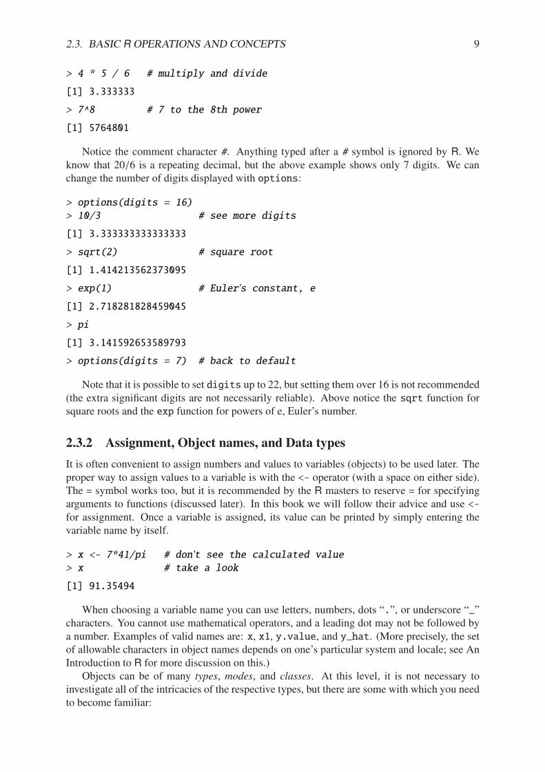
Notice the comment character #. Anything typed after a # symbol is ignored by R. Weknow that 20/6 is a repeating decimal, but the above example shows only 7 digits. We canchange the number of digits displayed with options:
> options(digits = 16)
> 10/3 # see more digits
[1] 3.333333333333333
> sqrt(2) # square root
[1] 1.414213562373095
> exp(1) # Euler's constant, e
[1] 2.718281828459045
> pi
[1] 3.141592653589793
> options(digits = 7) # back to default
Note that it is possible to set digits up to 22, but setting them over 16 is not recommended(the extra significant digits are not necessarily reliable). Above notice the sqrt function forsquare roots and the exp function for powers of e, Euler’s number.
2.3.2 Assignment, Object names, and Data types
It is often convenient to assign numbers and values to variables (objects) to be used later. Theproper way to assign values to a variable is with the <- operator (with a space on either side).The = symbol works too, but it is recommended by the R masters to reserve = for specifyingarguments to functions (discussed later). In this book we will follow their advice and use <-for assignment. Once a variable is assigned, its value can be printed by simply entering thevariable name by itself.
> x <- 7*41/pi # don't see the calculated value> x # take a look
[1] 91.35494
When choosing a variable name you can use letters, numbers, dots “.”, or underscore “_”characters. You cannot use mathematical operators, and a leading dot may not be followed bya number. Examples of valid names are: x, x1, y.value, and y_hat. (More precisely, the setof allowable characters in object names depends on one’s particular system and locale; see AnIntroduction to R for more discussion on this.)
Objects can be of many types, modes, and classes. At this level, it is not necessary toinvestigate all of the intricacies of the respective types, but there are some with which you needto become familiar:

10 CHAPTER 2. AN INTRODUCTION TO R
integer: the values 0, ±1, ±2, . . . ; these are represented exactly by R.
double: real numbers (rational and irrational); these numbers are not represented exactly (saveintegers or fractions with a denominator that is a multiple of 2, see [85]).
character: elements that are wrapped with pairs of " or ';
logical: includes TRUE, FALSE, and NA (which are reserved words); the NA stands for “notavailable”, i.e., a missing value.
You can determine an object’s type with the typeof function. In addition to the above, there isthe complex data type:
> sqrt(-1) # isn't defined
[1] NaN
> sqrt(-1+0i) # is defined
[1] 0+1i
> sqrt(as.complex(-1)) # same thing
[1] 0+1i
> (0 + 1i)^2 # should be -1
[1] -1+0i
> typeof((0 + 1i)^2)
[1] "complex"
Note that you can just type (1i)^2 to get the same answer. The NaN stands for “not anumber”; it is represented internally as double.
2.3.3 Vectors
All of this time we have been manipulating vectors of length 1. Now let us move to vectorswith multiple entries.
Entering data vectors
1. c: If you would like to enter the data 74,31,95,61,76,34,23,54,96 into R, you maycreate a data vector with the c function (which is short for concatenate).
> x <- c(74, 31, 95, 61, 76, 34, 23, 54, 96)
> x
[1] 74 31 95 61 76 34 23 54 96
The elements of a vector are usually coerced by R to the the most general type of any ofthe elements, so if you do c(1, "2") then the result will be c("1", "2").

2.3. BASIC R OPERATIONS AND CONCEPTS 11
2. scan: This method is useful when the data are stored somewhere else. For instance,you may type x <- scan() at the command prompt and R will display 1: to indicatethat it is waiting for the first data value. Type a value and press Enter, at which pointR will display 2:, and so forth. Note that entering an empty line stops the scan. Thismethod is especially handy when you have a column of values, say, stored in a text fileor spreadsheet. You may copy and paste them all at the 1: prompt, and R will store allof the values instantly in the vector x.
3. repeated data; regular patterns: the seq function will generate all sorts of sequencesof numbers. It has the arguments from, to, by, and length.out which can be set inconcert with one another. We will do a couple of examples to show you how it works.
> seq(from = 1, to = 5)
[1] 1 2 3 4 5
> seq(from = 2, by = -0.1, length.out = 4)
[1] 2.0 1.9 1.8 1.7
Note that we can get the first line much quicker with the colon operator :
> 1:5
[1] 1 2 3 4 5
The vector LETTERS has the 26 letters of the English alphabet in uppercase and lettershas all of them in lowercase.
Indexing data vectors Sometimes we do not want the whole vector, but just a piece of it. Wecan access the intermediate parts with the [] operator. Observe (with x defined above)
> x[1]
[1] 74
> x[2:4]
[1] 31 95 61
> x[c(1, 3, 4, 8)]
[1] 74 95 61 54
> x[-c(1, 3, 4, 8)]
[1] 31 76 34 23 96
Notice that we used the minus sign to specify those elements that we do not want.
> LETTERS[1:5]
[1] "A" "B" "C" "D" "E"
> letters[-(6:24)]
[1] "a" "b" "c" "d" "e" "y" "z"
12 CHAPTER 2. AN INTRODUCTION TO R
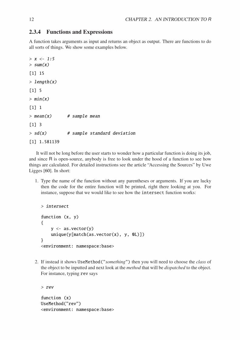
2.3.4 Functions and Expressions
A function takes arguments as input and returns an object as output. There are functions to doall sorts of things. We show some examples below.
> x <- 1:5
> sum(x)
[1] 15
> length(x)
[1] 5
> min(x)
[1] 1
> mean(x) # sample mean
[1] 3
> sd(x) # sample standard deviation
[1] 1.581139
It will not be long before the user starts to wonder how a particular function is doing its job,and since R is open-source, anybody is free to look under the hood of a function to see howthings are calculated. For detailed instructions see the article “Accessing the Sources” by UweLigges [60]. In short:
1. Type the name of the function without any parentheses or arguments. If you are luckythen the code for the entire function will be printed, right there looking at you. Forinstance, suppose that we would like to see how the intersect function works:
> intersect
function (x, y)
{
y <- as.vector(y)
unique(y[match(as.vector(x), y, 0L)])
}
<environment: namespace:base>
2. If instead it shows UseMethod("something") then you will need to choose the class ofthe object to be inputted and next look at themethod that will be dispatched to the object.For instance, typing rev says
> rev
function (x)
UseMethod("rev")
<environment: namespace:base>
2.3. BASIC R OPERATIONS AND CONCEPTS 13
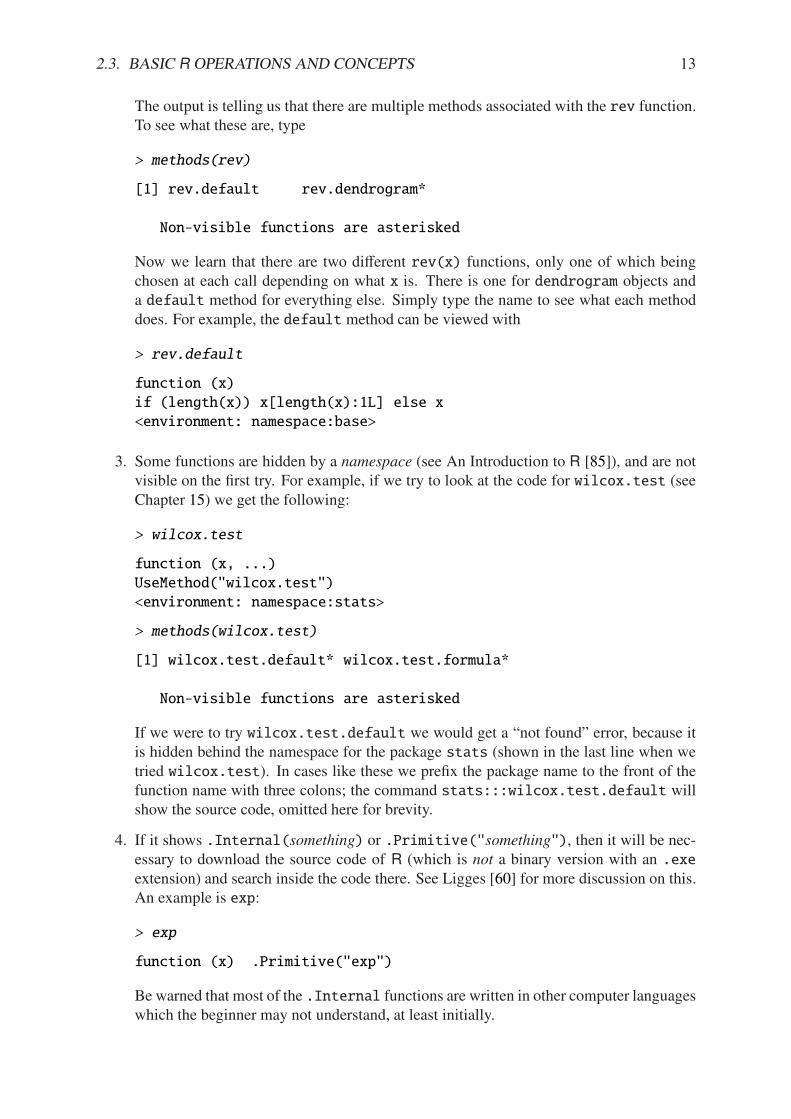
The output is telling us that there are multiple methods associated with the rev function.To see what these are, type
> methods(rev)
[1] rev.default rev.dendrogram*
Non-visible functions are asterisked
Now we learn that there are two di!erent rev(x) functions, only one of which beingchosen at each call depending on what x is. There is one for dendrogram objects anda default method for everything else. Simply type the name to see what each methoddoes. For example, the default method can be viewed with
> rev.default
function (x)
if (length(x)) x[length(x):1L] else x
<environment: namespace:base>
3. Some functions are hidden by a namespace (see An Introduction to R [85]), and are notvisible on the first try. For example, if we try to look at the code for wilcox.test (seeChapter 15) we get the following:
> wilcox.test
function (x, ...)
UseMethod("wilcox.test")
<environment: namespace:stats>
> methods(wilcox.test)
[1] wilcox.test.default* wilcox.test.formula*
Non-visible functions are asterisked
If we were to try wilcox.test.default we would get a “not found” error, because itis hidden behind the namespace for the package stats (shown in the last line when wetried wilcox.test). In cases like these we prefix the package name to the front of thefunction name with three colons; the command stats:::wilcox.test.default willshow the source code, omitted here for brevity.
4. If it shows .Internal(something) or .Primitive("something"), then it will be nec-essary to download the source code of R (which is not a binary version with an .exeextension) and search inside the code there. See Ligges [60] for more discussion on this.An example is exp:
> exp
function (x) .Primitive("exp")
Be warned that most of the .Internal functions are written in other computer languageswhich the beginner may not understand, at least initially.

14 CHAPTER 2. AN INTRODUCTION TO R
2.4 Getting Help
When you are using R, it will not take long before you find yourself needing help. Fortunately,R has extensive help resources and you should immediately become familiar with them. Beginby clicking Help on Rgui. The following options are available.
• Console: gives useful shortcuts, for instance, Ctrl+L, to clear the R console screen.
• FAQ on R: frequently asked questions concerning general R operation.
• FAQ on R for Windows: frequently asked questions about R, tailored to the MicrosoftWindows operating system.
• Manuals: technical manuals about all features of the R system including installation, thecomplete language definition, and add-on packages.
• R functions (text). . . : use this if you know the exact name of the function you want toknow more about, for example, mean or plot. Typing mean in the window is equivalentto typing help("mean") at the command line, or more simply, ?mean. Note that thismethod only works if the function of interest is contained in a package that is alreadyloaded into the search path with library.
• HTML Help: use this to browse the manuals with point-and-click links. It also has aSearch Engine & Keywords for searching the help page titles, with point-and-click linksfor the search results. This is possibly the best help method for beginners. It can bestarted from the command line with the command help.start().
• Search help. . . : use this if you do not know the exact name of the function of inter-est, or if the function is in a package that has not been loaded yet. For example, youmay enter plo and a text window will return listing all the help files with an alias, con-cept, or title matching ‘plo’ using regular expression matching; it is equivalent to typinghelp.search("plo") at the command line. The advantage is that you do not need toknow the exact name of the function; the disadvantage is that you cannot point-and-clickthe results. Therefore, one may wish to use the HTML Help search engine instead. Anequivalent way is ??plo at the command line.
• search.r-project.org. . . : this will search for words in help lists and email archives of theR Project. It can be very useful for finding other questions that other users have asked.
• Apropos. . . : use this for more sophisticated partial name matching of functions. See?apropos for details.
On the help pages for a function there are sometimes “Examples” listed at the bottom of thepage, which will work if copy-pasted at the command line (unless marked otherwise). Theexample function will run the code automatically, skipping the intermediate step. For instance,we may try example(mean) to see a few examples of how the mean function works.
2.4.1 R Help Mailing Lists
There are several mailing lists associated with R, and there is a huge community of people thatread and answer questions related to R. See here http://www.r-project.org/mail.html
2.5. EXTERNAL RESOURCES 15
for an idea of what is available. Particularly pay attention to the bottom of the page which listsseveral special interest groups (SIGs) related to R.
Bear in mind that R is free software, which means that it was written by volunteers, and thepeople that frequent the mailing lists are also volunteers who are not paid by customer supportfees. Consequently, if you want to use the mailing lists for free advice then you must adhere tosome basic etiquette, or else you may not get a reply, or even worse, you may receive a replywhich is a bit less cordial than you are used to. Below are a few considerations:
1. Read the FAQ (http://cran.r-project.org/faqs.html). Note that there are dif-ferent FAQs for di!erent operating systems. You should read these now, even without aquestion at the moment, to learn a lot about the idiosyncrasies of R.
2. Search the archives. Even if your question is not a FAQ, there is a very high likelihoodthat your question has been asked before on the mailing list. If you want to know abouttopic foo, then you can do RSiteSearch("foo") to search the mailing list archives(and the online help) for it.
3. Do a Google search and an RSeek.org search.
If your question is not a FAQ, has not been asked on R-help before, and does not yield to aGoogle (or alternative) search, then, and only then, should you even consider writing to R-help. Below are a few additional considerations.
1. Read the posting guide (http://www.r-project.org/posting-guide.html) be-fore posting. This will save you a lot of trouble and pain.
2. Get rid of the command prompts (>) from output. Readers of your message will take thetext from your mail and copy-paste into an R session. If you make the readers’ job easierthen it will increase the likelihood of a response.
3. Questions are often related to a specific data set, and the best way to communicate thedata is with a dump command. For instance, if your question involves data stored in avector x, you can type dump("x","") at the command prompt and copy-paste the outputinto the body of your email message. Then the reader may easily copy-paste the messagefrom your email into R and x will be available to him/her.
4. Sometimes the answer the question is related to the operating system used, the attachedpackages, or the exact version of R being used. The sessionInfo() command collectsall of this information to be copy-pasted into an email (and the Posting Guide requeststhis information). See Appendix A for an example.
2.5 External Resources
There is a mountain of information on the Internet about R. Below are a few of the importantones.
The R Project for Statistical Computing: (http://www.r-project.org/) Go here first.
The Comprehensive R Archive Network: (http://cran.r-project.org/) This is whereR is stored along with thousands of contributed packages. There are also loads of con-tributed information (books, tutorials, etc.). There are mirrors all over the world withduplicate information.

16 CHAPTER 2. AN INTRODUCTION TO R
R-Forge: (http://r-forge.r-project.org/) This is another location where R packagesare stored. Here you can find development code which has not yet been released toCRAN.
R Wiki: (http://wiki.r-project.org/rwiki/doku.php) There are many tips and trickslisted here. If you find a trick of your own, login and share it with the world.
Other: the R Graph Gallery (http://addictedtor.free.fr/graphiques/) and R Graph-ical Manual (http://bm2.genes.nig.ac.jp/RGM2/index.php) have literally thou-sands of graphs to peruse. RSeek (http://www.rseek.org) is a search engine basedon Google specifically tailored for R queries.
2.6 Other Tips
It is unnecessary to retype commands repeatedly, since R remembers what you have recentlyentered on the command line. On theMicrosoft!WindowsRGui, to cycle through the previouscommands just push the ! (up arrow) key. On Emacs/ESS the command is M-p (which meanshold down the Alt button and press “p”). More generally, the command history() will showa whole list of recently entered commands.
• To find out what all variables are in the current work environment, use the commandsobjects() or ls(). These list all available objects in the workspace. If you wish toremove one or more variables, use remove(var1, var2, var3), or more simply userm(var1, var2, var3), and to remove all objects use rm(list = ls()).
• Another use of scan is when you have a long list of numbers (separated by spaces or ondi!erent lines) already typed somewhere else, say in a text file. To enter all the data inone fell swoop, first highlight and copy the list of numbers to the Clipboard with Edit !Copy (or by right-clicking and selecting Copy). Next type the x <- scan() commandin the R console, and paste the numbers at the 1: prompt with Edit ! Paste. All of thenumbers will automatically be entered into the vector x.
• The command Ctrl+l clears the screen in the Microsoft!Windows RGui. The compa-rable command for Emacs/ESS is
• Once you use R for awhile there may be some commands that you wish to run automati-cally whenever R starts. These commands may be saved in a file called Rprofile.sitewhich is usually in the etc folder, which lives in the R home directory (which onMicrosoft!Windows usually is C:\Program Files\R). Alternatively, you can make afile .Rprofile to be stored in the user’s home directory, or anywhere R is invoked. Thisallows for multiple configurations for di!erent projects or users. See “Customizing theEnvironment” of An Introduction to R for more details.
• When exiting R the user is given the option to “save the workspace”. I recommend thatbeginners DO NOT save the workspace when quitting. If Yes is selected, then all ofthe objects and data currently in R’s memory is saved in a file located in the workingdirectory called .RData. This file is then automatically loaded the next time R starts(in which case R will say [previously saved workspace restored]). This is avaluable feature for experienced users of R, but I find that it causes more trouble than itsaves with beginners.

2.6. OTHER TIPS 17
Chapter Exercises

18 CHAPTER 2. AN INTRODUCTION TO R
Chapter 3
Data Description
In this chapter we introduce the di!erent types of data that a statistician is likely to encounter,and in each subsection we give some examples of how to display the data of that particular type.Once we see how to display data distributions, we next introduce the basic properties of datadistributions. We qualitatively explore several data sets. Once that we have intuitive propertiesof data sets, we next discuss how we may numerically measure and describe those propertieswith descriptive statistics.
What do I want them to know?
• di!erent data types, such as quantitative versus qualitative, nominal versus ordinal, anddiscrete versus continuous
• basic graphical displays for assorted data types, and some of their (dis)advantages
• fundamental properties of data distributions, including center, spread, shape, and crazyobservations
• methods to describe data (visually/numerically) with respect to the properties, and howthe methods di!er depending on the data type
• all of the above in the context of grouped data, and in particular, the concept of a factor
3.1 Types of Data
Loosely speaking, a datum is any piece of collected information, and a data set is a collectionof data related to each other in some way. We will categorize data into five types and describeeach in turn:
Quantitative data associated with a measurement of some quantity on an observational unit,
Qualitative data associated with some quality or property of the observational unit,
Logical data to represent true or false and which play an important role later,
Missing data that should be there but are not, and
Other types everything else under the sun.
In each subsection we look at some examples of the type in question and introduce methods todisplay them.
19
20 CHAPTER 3. DATA DESCRIPTION
3.1.1 Quantitative data
Quantitative data are any data that measure or are associated with a measurement of the quantityof something. They invariably assume numerical values. Quantitative data can be furthersubdivided into two categories.
• Discrete data take values in a finite or countably infinite set of numbers, that is, allpossible values could (at least in principle) be written down in an ordered list. Examplesinclude: counts, number of arrivals, or number of successes. They are often representedby integers, say, 0, 1, 2, etc..
• Continuous data take values in an interval of numbers. These are also known as scaledata, interval data, or measurement data. Examples include: height, weight, length, time,etc. Continuous data are often characterized by fractions or decimals: 3.82, 7.0001, 4 5
8,
etc..
Note that the distinction between discrete and continuous data is not always clear-cut. Some-times it is convenient to treat data as if they were continuous, even though strictly speakingthey are not continuous. See the examples.
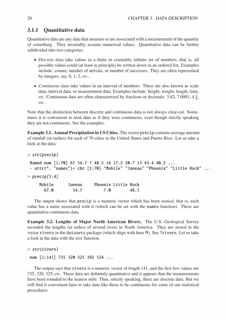
Example 3.1. Annual Precipitation in USCities. The vector precip contains average amountof rainfall (in inches) for each of 70 cities in the United States and Puerto Rico. Let us take alook at the data:
> str(precip)
Named num [1:70] 67 54.7 7 48.5 14 17.2 20.7 13 43.4 40.2 ...
- attr(*, "names")= chr [1:70] "Mobile" "Juneau" "Phoenix" "Little Rock" ...
> precip[1:4]
Mobile Juneau Phoenix Little Rock
67.0 54.7 7.0 48.5
The output shows that precip is a numeric vector which has been named, that is, eachvalue has a name associated with it (which can be set with the names function). These arequantitative continuous data.
Example 3.2. Lengths of Major North American Rivers. The U.S. Geological Surveyrecorded the lengths (in miles) of several rivers in North America. They are stored in thevector rivers in the datasets package (which ships with base R). See ?rivers. Let us takea look at the data with the str function.
> str(rivers)
num [1:141] 735 320 325 392 524 ...
The output says that rivers is a numeric vector of length 141, and the first few values are735, 320, 325, etc. These data are definitely quantitative and it appears that the measurementshave been rounded to the nearest mile. Thus, strictly speaking, these are discrete data. But wewill find it convenient later to take data like these to be continuous for some of our statisticalprocedures.
3.1. TYPES OF DATA 21
Example 3.3. Yearly Numbers of Important Discoveries. The vector discoveries containsnumbers of “great” inventions/discoveries in each year from 1860 to 1959, as reported by the1975 World Almanac. Let us take a look at the data:
> str(discoveries)
Time-Series [1:100] from 1860 to 1959: 5 3 0 2 0 3 2 3 6 1 ...
> discoveries[1:4]
[1] 5 3 0 2
The output is telling us that discoveries is a time series (see Section 3.1.5 for more) oflength 100. The entries are integers, and since they represent counts this is a good example ofdiscrete quantitative data. We will take a closer look in the following sections.
Displaying Quantitative Data
One of the first things to do when confronted by quantitative data (or any data, for that matter)is to make some sort of visual display to gain some insight into the data’s structure. There arealmost as many display types from which to choose as there are data sets to plot. We describesome of the more popular alternatives.
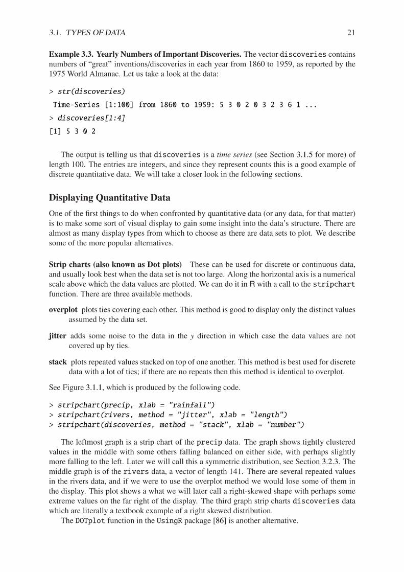
Strip charts (also known as Dot plots) These can be used for discrete or continuous data,and usually look best when the data set is not too large. Along the horizontal axis is a numericalscale above which the data values are plotted. We can do it in R with a call to the stripchartfunction. There are three available methods.
overplot plots ties covering each other. This method is good to display only the distinct valuesassumed by the data set.
jitter adds some noise to the data in the y direction in which case the data values are notcovered up by ties.
stack plots repeated values stacked on top of one another. This method is best used for discretedata with a lot of ties; if there are no repeats then this method is identical to overplot.
See Figure 3.1.1, which is produced by the following code.
> stripchart(precip, xlab = "rainfall")
> stripchart(rivers, method = "jitter", xlab = "length")
> stripchart(discoveries, method = "stack", xlab = "number")
The leftmost graph is a strip chart of the precip data. The graph shows tightly clusteredvalues in the middle with some others falling balanced on either side, with perhaps slightlymore falling to the left. Later we will call this a symmetric distribution, see Section 3.2.3. Themiddle graph is of the rivers data, a vector of length 141. There are several repeated valuesin the rivers data, and if we were to use the overplot method we would lose some of them inthe display. This plot shows a what we will later call a right-skewed shape with perhaps someextreme values on the far right of the display. The third graph strip charts discoveries datawhich are literally a textbook example of a right skewed distribution.
The DOTplot function in the UsingR package [86] is another alternative.
22 CHAPTER 3. DATA DESCRIPTION
10 30 50
rainfall
0 1000 2500
length
0 2 4 6 8 12
number
Figure 3.1.1: Strip charts of the precip, rivers, and discoveries data
The first graph uses the overplot method, the second the jitter method, and the third the stack
method.
3.1. TYPES OF DATA 23
precip
Fre
quency
0 20 40 60
05
10
15
20
25
precip
Densi
ty
0 20 40 600
.000
0.0
10
0.0
20
0.0
30
Figure 3.1.2: (Relative) frequency histograms of the precip data
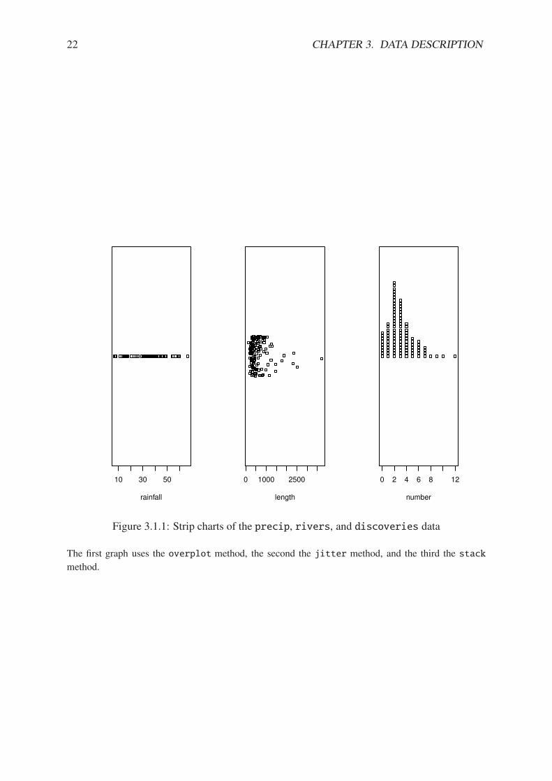
Histogram These are typically used for continuous data. A histogram is constructed by firstdeciding on a set of classes, or bins, which partition the real line into a set of boxes into whichthe data values fall. Then vertical bars are drawn over the bins with height proportional to thenumber of observations that fell into the bin.
These are one of the most common summary displays, and they are often misidentified as“Bar Graphs” (see below.) The scale on the y axis can be frequency, percentage, or density(relative frequency). The term histogram was coined by Karl Pearson in 1891, see [66].
Example 3.4. Annual Precipitation in US Cities. We are going to take another look at theprecip data that we investigated earlier. The strip chart in Figure 3.1.1 suggested a looselybalanced distribution; let us now look to see what a histogram says.
There are many ways to plot histograms in R, and one of the easiest is with the histfunction. The following code produces the plots in Figure 3.1.2.
> hist(precip, main = "")
> hist(precip, freq = FALSE, main = "")
Notice the argument main = "", which suppresses the main title from being displayed– it would have said “Histogram of precip” otherwise. The plot on the left is a frequencyhistogram (the default), and the plot on the right is a relative frequency histogram (freq =FALSE).
Please be careful regarding the biggest weakness of histograms: the graph obtained stronglydepends on the bins chosen. Choose another set of bins, and you will get a di!erent histogram.
24 CHAPTER 3. DATA DESCRIPTION
precip
Fre
quency
10 30 50 70
02
46
810
12
14
precip
Fre
quency
10 30 500
12
34
Figure 3.1.3: More histograms of the precip data
Moreover, there are not any definitive criteria by which bins should be defined; the best choicefor a given data set is the one which illuminates the data set’s underlying structure (if any).Luckily for us there are algorithms to automatically choose bins that are likely to display well,and more often than not the default bins do a good job. This is not always the case, however, anda responsible statistician will investigate many bin choices to test the stability of the display.
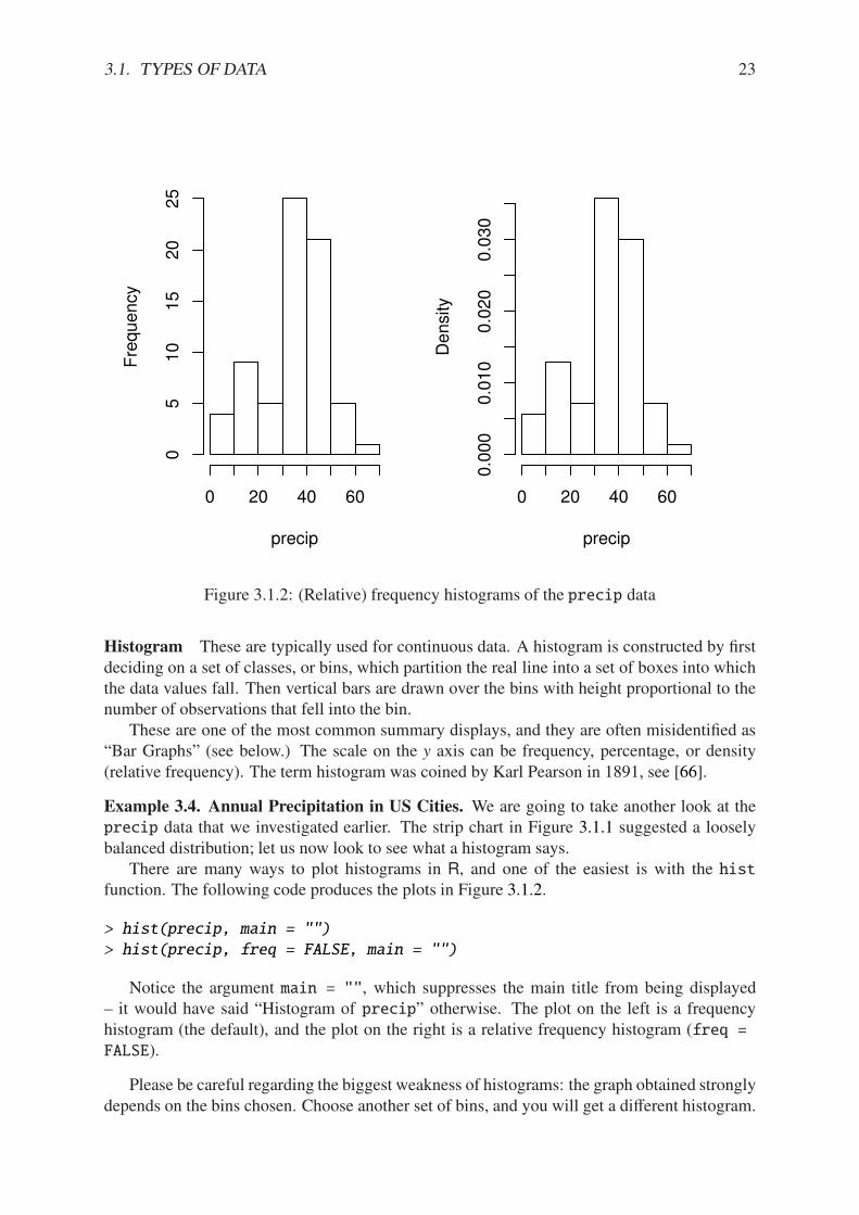
Example 3.5. Recall that the strip chart in Figure 3.1.1 suggested a relatively balanced shapeto the precip data distribution. Watch what happens when we change the bins slightly (withthe breaks argument to hist). See Figure 3.1.3 which was produced by the following code.
> hist(precip, breaks = 10, main = "")
> hist(precip, breaks = 200, main = "")
The leftmost graph (with breaks = 10) shows that the distribution is not balanced at all.There are two humps: a big one in the middle and a smaller one to the left. Graphs like thisoften indicate some underlying group structure to the data; we could now investigate whetherthe cities for which rainfall was measured were similar in some way, with respect to geographicregion, for example.
The rightmost graph in Figure 3.1.3 shows what happens when the number of bins is toolarge: the histogram is too grainy and hides the rounded appearance of the earlier histograms.If we were to continue increasing the number of bins we would eventually get all observed binsto have exactly one element, which is nothing more than a glorified strip chart.
3.1. TYPES OF DATA 25
Stemplots (more to be said in Section 3.4) Stemplots have two basic parts: stems and leaves.The final digit of the data values is taken to be a leaf, and the leading digit(s) is (are) taken tobe stems. We draw a vertical line, and to the left of the line we list the stems. To the right of theline, we list the leaves beside their corresponding stem. There will typically be several leavesfor each stem, in which case the leaves accumulate to the right. It is sometimes necessary toround the data values, especially for larger data sets.
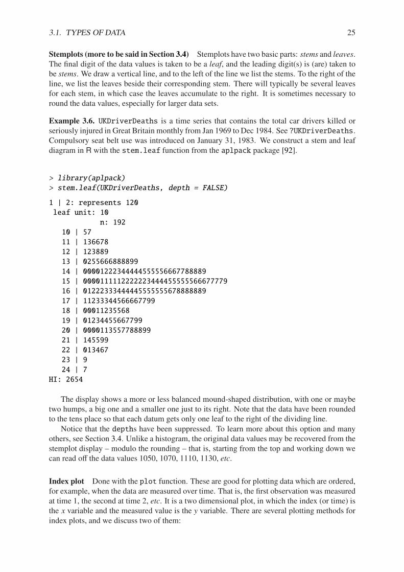
Example 3.6. UKDriverDeaths is a time series that contains the total car drivers killed orseriously injured in Great Britain monthly from Jan 1969 to Dec 1984. See ?UKDriverDeaths.Compulsory seat belt use was introduced on January 31, 1983. We construct a stem and leafdiagram in R with the stem.leaf function from the aplpack package [92].
> library(aplpack)
> stem.leaf(UKDriverDeaths, depth = FALSE)
1 | 2: represents 120
leaf unit: 10
n: 192
10 | 57
11 | 136678
12 | 123889
13 | 0255666888899
14 | 00001222344444555556667788889
15 | 0000111112222223444455555566677779
16 | 01222333444445555555678888889
17 | 11233344566667799
18 | 00011235568
19 | 01234455667799
20 | 0000113557788899
21 | 145599
22 | 013467
23 | 9
24 | 7
HI: 2654
The display shows a more or less balanced mound-shaped distribution, with one or maybetwo humps, a big one and a smaller one just to its right. Note that the data have been roundedto the tens place so that each datum gets only one leaf to the right of the dividing line.
Notice that the depths have been suppressed. To learn more about this option and manyothers, see Section 3.4. Unlike a histogram, the original data values may be recovered from thestemplot display – modulo the rounding – that is, starting from the top and working down wecan read o! the data values 1050, 1070, 1110, 1130, etc.
Index plot Done with the plot function. These are good for plotting data which are ordered,for example, when the data are measured over time. That is, the first observation was measuredat time 1, the second at time 2, etc. It is a two dimensional plot, in which the index (or time) isthe x variable and the measured value is the y variable. There are several plotting methods forindex plots, and we discuss two of them:
26 CHAPTER 3. DATA DESCRIPTION
spikes: draws a vertical line from the x-axis to the observation height (type = "h").
points: plots a simple point at the observation height (type = "p").
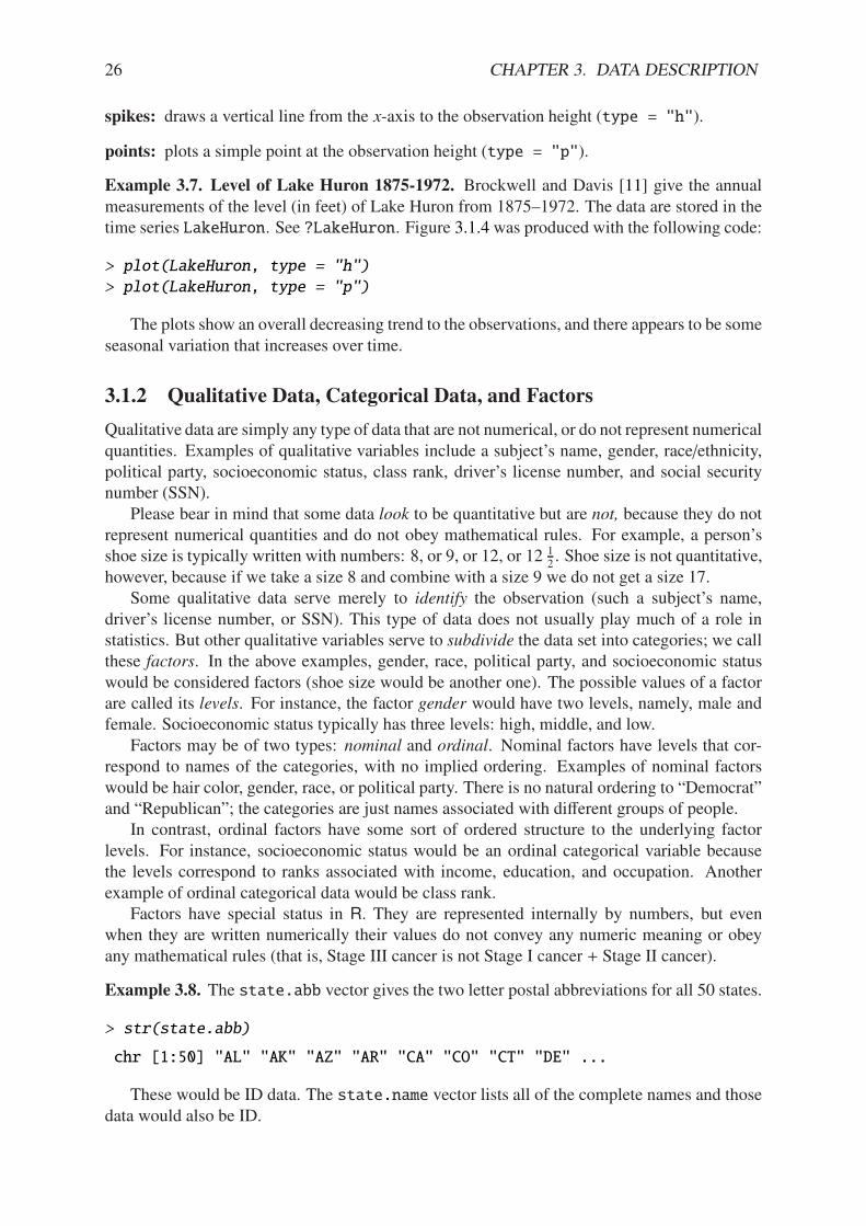
Example 3.7. Level of Lake Huron 1875-1972. Brockwell and Davis [11] give the annualmeasurements of the level (in feet) of Lake Huron from 1875–1972. The data are stored in thetime series LakeHuron. See ?LakeHuron. Figure 3.1.4 was produced with the following code:
> plot(LakeHuron, type = "h")
> plot(LakeHuron, type = "p")
The plots show an overall decreasing trend to the observations, and there appears to be someseasonal variation that increases over time.
3.1.2 Qualitative Data, Categorical Data, and Factors
Qualitative data are simply any type of data that are not numerical, or do not represent numericalquantities. Examples of qualitative variables include a subject’s name, gender, race/ethnicity,political party, socioeconomic status, class rank, driver’s license number, and social securitynumber (SSN).
Please bear in mind that some data look to be quantitative but are not, because they do notrepresent numerical quantities and do not obey mathematical rules. For example, a person’sshoe size is typically written with numbers: 8, or 9, or 12, or 12 1
2. Shoe size is not quantitative,
however, because if we take a size 8 and combine with a size 9 we do not get a size 17.Some qualitative data serve merely to identify the observation (such a subject’s name,
driver’s license number, or SSN). This type of data does not usually play much of a role instatistics. But other qualitative variables serve to subdivide the data set into categories; we callthese factors. In the above examples, gender, race, political party, and socioeconomic statuswould be considered factors (shoe size would be another one). The possible values of a factorare called its levels. For instance, the factor gender would have two levels, namely, male andfemale. Socioeconomic status typically has three levels: high, middle, and low.
Factors may be of two types: nominal and ordinal. Nominal factors have levels that cor-respond to names of the categories, with no implied ordering. Examples of nominal factorswould be hair color, gender, race, or political party. There is no natural ordering to “Democrat”and “Republican”; the categories are just names associated with di!erent groups of people.
In contrast, ordinal factors have some sort of ordered structure to the underlying factorlevels. For instance, socioeconomic status would be an ordinal categorical variable becausethe levels correspond to ranks associated with income, education, and occupation. Anotherexample of ordinal categorical data would be class rank.
Factors have special status in R. They are represented internally by numbers, but evenwhen they are written numerically their values do not convey any numeric meaning or obeyany mathematical rules (that is, Stage III cancer is not Stage I cancer + Stage II cancer).
Example 3.8. The state.abb vector gives the two letter postal abbreviations for all 50 states.
> str(state.abb)
chr [1:50] "AL" "AK" "AZ" "AR" "CA" "CO" "CT" "DE" ...
These would be ID data. The state.name vector lists all of the complete names and thosedata would also be ID.
3.1. TYPES OF DATA 27
Time
Lake
Huro
n
1880 1900 1920 1940 1960
576
578
580
582
Time
Lake
Huro
n
1880 1900 1920 1940 1960
576
578
580
582
Figure 3.1.4: Index plots of the LakeHuron data

28 CHAPTER 3. DATA DESCRIPTION
Example 3.9. U.S. State Facts and Features. The U.S. Department of Commerce of theU.S. Census Bureau releases all sorts of information in the Statistical Abstract of the United
States, and the state.region data lists each of the 50 states and the region to which it belongs,be it Northeast, South, North Central, or West. See ?state.region.
> str(state.region)
Factor w/ 4 levels "Northeast","South",..: 2 4 4 2 4 4 1 2 2 2 ...
> state.region[1:5]
[1] South West West South West
Levels: Northeast South North Central West
The str output shows that state.region is already stored internally as a factor and it listsa couple of the factor levels. To see all of the levels we printed the first five entries of the vectorin the second line.need to print a piece of the from
Displaying Qualitative Data
Tables One of the best ways to summarize qualitative data is with a table of the data values.We may count frequencies with the table function or list proportions with the prop.tablefunction (whose input is a frequency table). In the R Commander you can do it with Statistics !Frequency Distribution. . . . Alternatively, to look at tables for all factors in the Active dataset you can do Statistics ! Summaries ! Active Dataset.
> Tbl <- table(state.division)
> Tbl # frequencies
state.division
New England Middle Atlantic South Atlantic
6 3 8
East South Central West South Central East North Central
4 4 5
West North Central Mountain Pacific
7 8 5
> Tbl/sum(Tbl) # relative frequencies
state.division
New England Middle Atlantic South Atlantic
0.12 0.06 0.16
East South Central West South Central East North Central
0.08 0.08 0.10
West North Central Mountain Pacific
0.14 0.16 0.10
> prop.table(Tbl) # same thing
state.division
New England Middle Atlantic South Atlantic
0.12 0.06 0.16
East South Central West South Central East North Central
0.08 0.08 0.10
West North Central Mountain Pacific
0.14 0.16 0.10
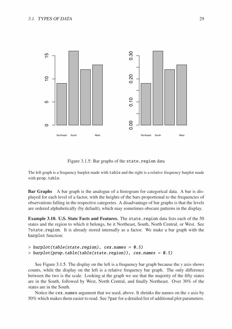
3.1. TYPES OF DATA 29
Northeast South West
05
10
15
Northeast South West
0.0
00.1
00.2
00.3
0
Figure 3.1.5: Bar graphs of the state.region data
The left graph is a frequency barplot made with table and the right is a relative frequency barplot made
with prop.table.
Bar Graphs A bar graph is the analogue of a histogram for categorical data. A bar is dis-played for each level of a factor, with the heights of the bars proportional to the frequencies ofobservations falling in the respective categories. A disadvantage of bar graphs is that the levelsare ordered alphabetically (by default), which may sometimes obscure patterns in the display.
Example 3.10. U.S. State Facts and Features. The state.region data lists each of the 50states and the region to which it belongs, be it Northeast, South, North Central, or West. See?state.region. It is already stored internally as a factor. We make a bar graph with thebarplot function:
> barplot(table(state.region), cex.names = 0.5)
> barplot(prop.table(table(state.region)), cex.names = 0.5)
See Figure 3.1.5. The display on the left is a frequency bar graph because the y axis showscounts, while the display on the left is a relative frequency bar graph. The only di!erencebetween the two is the scale. Looking at the graph we see that the majority of the fifty statesare in the South, followed by West, North Central, and finally Northeast. Over 30% of thestates are in the South.
Notice the cex.names argument that we used, above. It shrinks the names on the x axis by50%which makes them easier to read. See ?par for a detailed list of additional plot parameters.
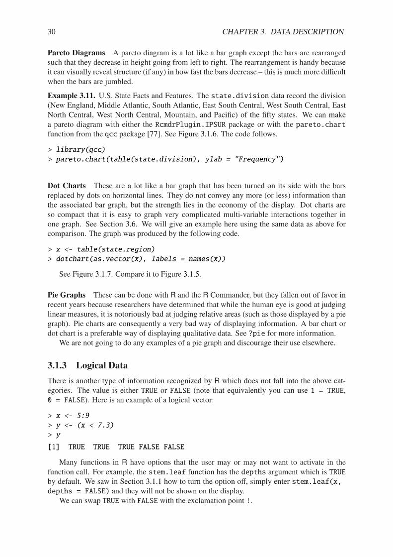
30 CHAPTER 3. DATA DESCRIPTION
Pareto Diagrams A pareto diagram is a lot like a bar graph except the bars are rearrangedsuch that they decrease in height going from left to right. The rearrangement is handy becauseit can visually reveal structure (if any) in how fast the bars decrease – this is much more di"cultwhen the bars are jumbled.
Example 3.11. U.S. State Facts and Features. The state.division data record the division(New England, Middle Atlantic, South Atlantic, East South Central, West South Central, EastNorth Central, West North Central, Mountain, and Pacific) of the fifty states. We can makea pareto diagram with either the RcmdrPlugin.IPSUR package or with the pareto.chartfunction from the qcc package [77]. See Figure 3.1.6. The code follows.
> library(qcc)
> pareto.chart(table(state.division), ylab = "Frequency")
Dot Charts These are a lot like a bar graph that has been turned on its side with the barsreplaced by dots on horizontal lines. They do not convey any more (or less) information thanthe associated bar graph, but the strength lies in the economy of the display. Dot charts areso compact that it is easy to graph very complicated multi-variable interactions together inone graph. See Section 3.6. We will give an example here using the same data as above forcomparison. The graph was produced by the following code.
> x <- table(state.region)
> dotchart(as.vector(x), labels = names(x))
See Figure 3.1.7. Compare it to Figure 3.1.5.
Pie Graphs These can be done with R and the R Commander, but they fallen out of favor inrecent years because researchers have determined that while the human eye is good at judginglinear measures, it is notoriously bad at judging relative areas (such as those displayed by a piegraph). Pie charts are consequently a very bad way of displaying information. A bar chart ordot chart is a preferable way of displaying qualitative data. See ?pie for more information.
We are not going to do any examples of a pie graph and discourage their use elsewhere.
3.1.3 Logical Data
There is another type of information recognized by R which does not fall into the above cat-egories. The value is either TRUE or FALSE (note that equivalently you can use 1 = TRUE,0 = FALSE). Here is an example of a logical vector:
> x <- 5:9
> y <- (x < 7.3)
> y
[1] TRUE TRUE TRUE FALSE FALSE
Many functions in R have options that the user may or may not want to activate in thefunction call. For example, the stem.leaf function has the depths argument which is TRUEby default. We saw in Section 3.1.1 how to turn the option o!, simply enter stem.leaf(x,depths = FALSE) and they will not be shown on the display.
We can swap TRUE with FALSE with the exclamation point !.

3.1. TYPES OF DATA 31
Package 'qcc', version 2.0.1
Type 'citation("qcc")' for citing this R package in publications.
Pareto chart analysis for table(state.division)
Frequency Cum.Freq. Percentage Cum.Percent.
Mountain 8 8 16 16
South Atlantic 8 16 16 32
West North Central 7 23 14 46
New England 6 29 12 58
Pacific 5 34 10 68
East North Central 5 39 10 78
West South Central 4 43 8 86
East South Central 4 47 8 94
Middle Atlantic 3 50 6 100
Mou
nta
in
South
Atla
ntic
West
Nort
h C
entr
al
New
Engla
nd
Paci
fic
East
Nort
h C
entr
al
West
South
Ce
ntr
al
East
South
Ce
ntr
al
Mid
dle
Atla
ntic
Pareto Chart for table(state.division)
Fre
quency
010
20
30
40
50
0%
25%
75%
Cum
ula
tive P
erc
enta
ge
Figure 3.1.6: Pareto chart of the state.division data
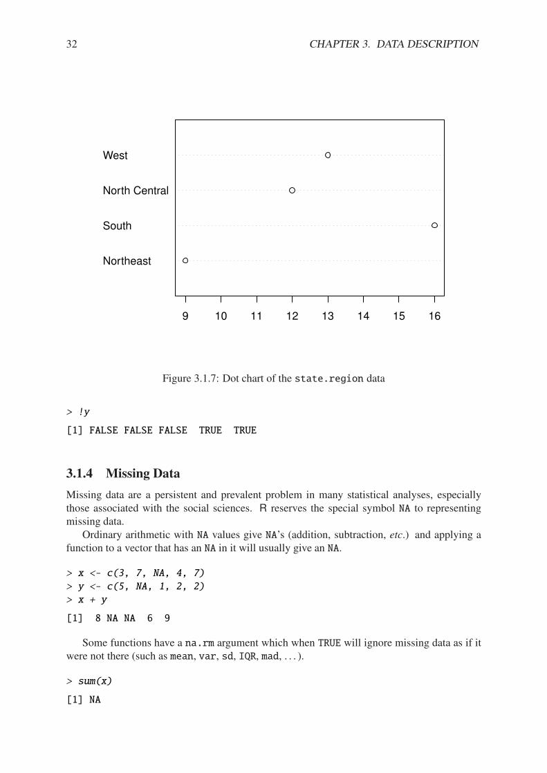
32 CHAPTER 3. DATA DESCRIPTION
Northeast
South
North Central
West
9 10 11 12 13 14 15 16
Figure 3.1.7: Dot chart of the state.region data
> !y
[1] FALSE FALSE FALSE TRUE TRUE
3.1.4 Missing Data
Missing data are a persistent and prevalent problem in many statistical analyses, especiallythose associated with the social sciences. R reserves the special symbol NA to representingmissing data.
Ordinary arithmetic with NA values give NA’s (addition, subtraction, etc.) and applying afunction to a vector that has an NA in it will usually give an NA.
> x <- c(3, 7, NA, 4, 7)
> y <- c(5, NA, 1, 2, 2)
> x + y
[1] 8 NA NA 6 9
Some functions have a na.rm argument which when TRUE will ignore missing data as if itwere not there (such as mean, var, sd, IQR, mad, . . . ).
> sum(x)
[1] NA
3.2. FEATURES OF DATA DISTRIBUTIONS 33
> sum(x, na.rm = TRUE)
[1] 21
Other functions do not have a na.rm argument and will return NA or an error if the argumenthas NAs. In those cases we can find the locations of any NAs with the is.na function and removethose cases with the [] operator.
> is.na(x)
[1] FALSE FALSE TRUE FALSE FALSE
> z <- x[!is.na(x)]
> sum(z)
[1] 21
The analogue of is.na for rectangular data sets (or data frames) is the complete.casesfunction. See Appendix D.4.
3.1.5 Other Data Types
3.2 Features of Data Distributions
Given that the data have been appropriately displayed, the next step is to try to identify salientfeatures represented in the graph. The acronym to remember is Center, Unusual features,Spread, and Shape. (CUSS).
3.2.1 Center
One of the most basic features of a data set is its center. Loosely speaking, the center of a dataset is associated with a number that represents a middle or general tendency of the data. Ofcourse, there are usually several values that would serve as a center, and our later tasks will befocused on choosing an appropriate one for the data at hand. Judging from the histogram thatwe saw in Figure 3.1.3, a measure of center would be about 35.
3.2.2 Spread
The spread of a data set is associated with its variability; data sets with a large spread tend tocover a large interval of values, while data sets with small spread tend to cluster tightly arounda central value.
3.2.3 Shape
When we speak of the shape of a data set, we are usually referring to the shape exhibited byan associated graphical display, such as a histogram. The shape can tell us a lot about anyunderlying structure to the data, and can help us decide which statistical procedure we shoulduse to analyze them.
34 CHAPTER 3. DATA DESCRIPTION
Symmetry and Skewness A distribution is said to be right-skewed (or positively skewed)if the right tail seems to be stretched from the center. A left-skewed (or negatively skewed)distribution is stretched to the left side. A symmetric distribution has a graph that is balancedabout its center, in the sense that half of the graph may be reflected about a central line ofsymmetry to match the other half.
We have already encountered skewed distributions: both the discoveries data in Figure3.1.1 and the precip data in Figure 3.1.3 appear right-skewed. The UKDriverDeaths data inExample 3.6 is relatively symmetric (but note the one extreme value 2654 identified at thebottom of the stemplot).
Kurtosis Another component to the shape of a distribution is how “peaked” it is. Some dis-tributions tend to have a flat shape with thin tails. These are called platykurtic, and an exampleof a platykurtic distribution is the uniform distribution; see Section 6.2. On the other end ofthe spectrum are distributions with a steep peak, or spike, accompanied by heavy tails; theseare called leptokurtic. Examples of leptokurtic distributions are the Laplace distribution andthe logistic distribution. See Section 6.5. In between are distributions (called mesokurtic) witha rounded peak and moderately sized tails. The standard example of a mesokurtic distributionis the famous bell-shaped curve, also known as the Gaussian, or normal, distribution, and thebinomial distribution can be mesokurtic for specific choices of p. See Sections 5.3 and 6.3.
3.2.4 Clusters and Gaps
Clusters or gaps are sometimes observed in quantitative data distributions. They indicateclumping of the data about distinct values, and gaps may exist between clusters. Clustersoften suggest an underlying grouping to the data. For example, take a look at the faithfuldata which contains the duration of eruptions and the waiting time between eruptions ofthe Old Faithful geyser in Yellowstone National Park. (Do not be frightened by the complicatedinformation at the left of the display for now; we will learn how to interpret it in Section 3.4).
> library(aplpack)
> stem.leaf(faithful$eruptions)
1 | 2: represents 1.2
leaf unit: 0.1
n: 272
12 s | 667777777777
51 1. | 888888888888888888888888888899999999999
71 2* | 00000000000011111111
87 t | 2222222222333333
92 f | 44444
94 s | 66
97 2. | 889
98 3* | 0
102 t | 3333
108 f | 445555
118 s | 6666677777
(16) 3. | 8888888889999999
138 4* | 0000000000000000111111111111111
107 t | 22222222222233333333333333333
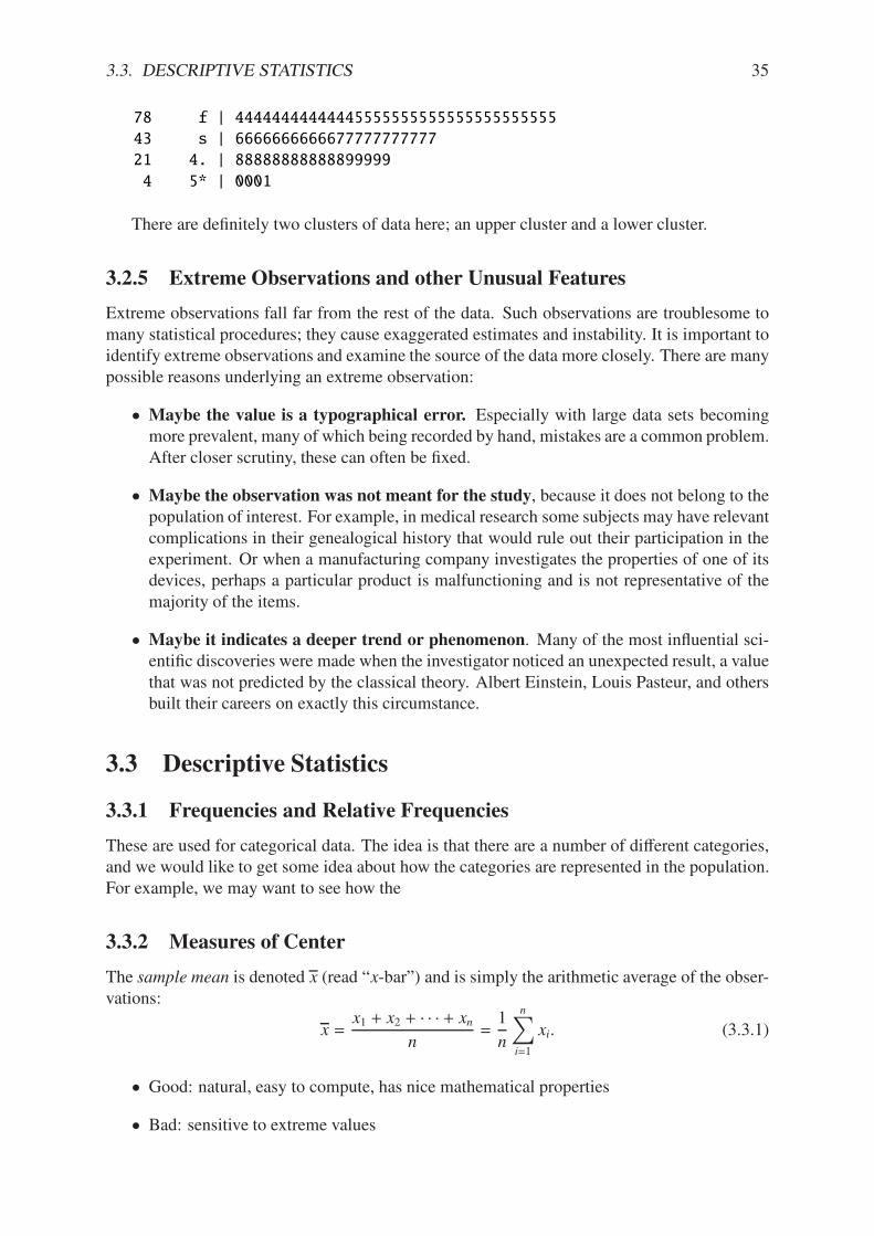
3.3. DESCRIPTIVE STATISTICS 35
78 f | 44444444444445555555555555555555555
43 s | 6666666666677777777777
21 4. | 88888888888899999
4 5* | 0001
There are definitely two clusters of data here; an upper cluster and a lower cluster.
3.2.5 Extreme Observations and other Unusual Features
Extreme observations fall far from the rest of the data. Such observations are troublesome tomany statistical procedures; they cause exaggerated estimates and instability. It is important toidentify extreme observations and examine the source of the data more closely. There are manypossible reasons underlying an extreme observation:
• Maybe the value is a typographical error. Especially with large data sets becomingmore prevalent, many of which being recorded by hand, mistakes are a common problem.After closer scrutiny, these can often be fixed.
• Maybe the observation was not meant for the study, because it does not belong to thepopulation of interest. For example, in medical research some subjects may have relevantcomplications in their genealogical history that would rule out their participation in theexperiment. Or when a manufacturing company investigates the properties of one of itsdevices, perhaps a particular product is malfunctioning and is not representative of themajority of the items.
• Maybe it indicates a deeper trend or phenomenon. Many of the most influential sci-entific discoveries were made when the investigator noticed an unexpected result, a valuethat was not predicted by the classical theory. Albert Einstein, Louis Pasteur, and othersbuilt their careers on exactly this circumstance.
3.3 Descriptive Statistics
3.3.1 Frequencies and Relative Frequencies
These are used for categorical data. The idea is that there are a number of di!erent categories,and we would like to get some idea about how the categories are represented in the population.For example, we may want to see how the
3.3.2 Measures of Center
The sample mean is denoted x (read “x-bar”) and is simply the arithmetic average of the obser-vations:
x =x1 + x2 + · · · + xn
n=
1
n
n!
i=1
xi. (3.3.1)
• Good: natural, easy to compute, has nice mathematical properties
• Bad: sensitive to extreme values
36 CHAPTER 3. DATA DESCRIPTION
It is appropriate for use with data sets that are not highly skewed without extreme observations.The sample median is another popular measure of center and is denoted x. To calculate
its value, first sort the data into an increasing sequence of numbers. If the data set has an oddnumber of observations then x is the value of the middle observation, which lies in position(n + 1)/2; otherwise, there are two middle observations and x is the average of those middlevalues.
• Good: resistant to extreme values, easy to describe
• Bad: not as mathematically tractable, need to sort the data to calculate
One desirable property of the sample median is that it is resistant to extreme observations, inthe sense that the value of x depends only the values of the middle observations, and is quiteuna!ected by the actual values of the outer observations in the ordered list. The same cannotbe said for the sample mean. Any significant changes in the magnitude of an observation xkresults in a corresponding change in the value of the mean. Hence, the sample mean is said tobe sensitive to extreme observations.
The trimmed mean is a measure designed to address the sensitivity of the sample mean toextreme observations. The idea is to “trim” a fraction (less than 1/2) of the observations o!each end of the ordered list, and then calculate the sample mean of what remains. We willdenote it by xt=0.05.
• Good: resistant to extreme values, shares nice statistical properties
• Bad: need to sort the data
3.3.3 How to do it with R
• You can calculate frequencies or relative frequencies with the table function, and rela-tive frequencies with prop.table(table()).
• You can calculate the sample mean of a data vector x with the command mean(x).
• You can calculate the sample median of x with the command median(x).
• You can calculate the trimmedmean with the trim argument; mean(x, trim = 0.05).
3.3.4 Order Statistics and the Sample Quantiles
A common first step in an analysis of a data set is to sort the values. Given a data set x1, x2,. . . ,xn, we may sort the values to obtain an increasing sequence
x(1) " x(2) " x(3) " · · · " x(n) (3.3.2)
and the resulting values are called the order statistics. The kth entry in the list, x(k), is the kth
order statistic, and approximately 100(k/n)% of the observations fall below x(k). The orderstatistics give an indication of the shape of the data distribution, in the sense that a person canlook at the order statistics and have an idea about where the data are concentrated, and wherethey are sparse.
The sample quantiles are related to the order statistics. Unfortunately, there is not a uni-versally accepted definition of them. Indeed, R is equipped to calculate quantiles using nine
3.3. DESCRIPTIVE STATISTICS 37
distinct definitions! We will describe the default method (type = 7), but the interested readercan see the details for the other methods with ?quantile.
Suppose the data set has n observations. Find the sample quantile of order p (0 < p < 1),denoted qp , as follows:
First step: sort the data to obtain the order statistics x(1), x(2), . . . ,x(n).
Second step: calculate (n # 1)p + 1 and write it in the form k.d, where k is an integer and d isa decimal.
Third step: The sample quantile qp is
qp = x(k) + d(x(k+1) # x(k)). (3.3.3)
The interpretation of qp is that approximately 100p% of the data fall below the value qp .Keep in mind that there is not a unique definition of percentiles, quartiles, etc. Open a
di!erent book, and you’ll find a di!erent procedure. The di!erence is small and seldom playsa role except in small data sets with repeated values. In fact, most people do not even notice incommon use.
Clearly, the most popular sample quantile is q0.50, also known as the sample median, x. Theclosest runners-up are the first quartile q0.25 and the third quartile q0.75 (the second quartile isthe median).
3.3.5 How to do it with R
At the command prompt We can find the order statistics of a data set stored in a vector xwith the command sort(x).
You can calculate the sample quantiles of any order p where 0 < p < 1 for a data set storedin a data vector x with the quantile function, for instance, the command quantile(x,probs = c(0, 0.25, 0.37)) will return the smallest observation, the first quartile, q0.25,and the 37th sample quantile, q0.37. For qp simply change the values in the probs argument tothe value p.
With the R Commander In Rcmdr we can find the order statistics of a variable in theActive data set by doing Data ! Manage variables in Active data set. . . ! Computenew variable. . . . In the Expression to compute dialog simply type sort(varname), wherevarname is the variable that it is desired to sort.
In Rcmdr, we can calculate the sample quantiles for a particular variable with the sequenceStatistics ! Summaries ! Numerical Summaries. . . . We can automatically calculate the quar-tiles for all variables in the Active data set with the sequence Statistics ! Summaries !Active Dataset.
3.3.6 Measures of Spread
Sample Variance and Standard Deviation The sample variance is denoted s2 and is calcu-lated with the formula
s2 =1
n # 1
n!
i=1
(xi # x)2. (3.3.4)
38 CHAPTER 3. DATA DESCRIPTION
The sample standard deviation is s =$s2. Intuitively, the sample variance is approximately
the average squared distance of the observations from the sample mean. The sample standarddeviation is used to scale the estimate back to the measurement units of the original data.
• Good: tractable, has nice mathematical/statistical properties
• Bad: sensitive to extreme values
We will spend a lot of time with the variance and standard deviation in the coming chapters.In the meantime, the following two rules give some meaning to the standard deviation, in thatthere are bounds on how much of the data can fall past a certain distance from the mean.
Fact 3.12. Chebychev’s Rule: The proportion of observations within k standard deviations of
the mean is at least 1 # 1/k2, i.e., at least 75%, 89%, and 94% of the data are within 2, 3, and
4 standard deviations of the mean, respectively.
Note that Chebychev’s Rule does not say anything about when k = 1, because 1#1/12 = 0,which states that at least 0% of the observations are within one standard deviation of the mean(which is not saying much).
Chebychev’s Rule applies to any data distribution, any list of numbers, no matter where itcame from or what the histogram looks like. The price for such generality is that the boundsare not very tight; if we know more about how the data are shaped then we can say more abouthow much of the data can fall a given distance from the mean.
Fact 3.13. Empirical Rule: If data follow a bell-shaped curve, then approximately 68%, 95%,
and 99.7% of the data are within 1, 2, and 3 standard deviations of the mean, respectively.
Interquartile Range Just as the sample mean is sensitive to extreme values, so the associatedmeasure of spread is similarly sensitive to extremes. Further, the problem is exacerbated by thefact that the extreme distances are squared. We know that the sample quartiles are resistantto extremes, and a measure of spread associated with them is the interquartile range (IQR)defined by IQR = q0.75 # q0.25.
• Good: stable, resistant to outliers, robust to nonnormality, easy to explain
• Bad: not as tractable, need to sort the data, only involves the middle 50% of the data.
Median Absolute Deviation A measure even more robust than the IQR is the median abso-
lute deviation (MAD). To calculate it we first get the median "x, next the absolute deviations
|x1 # x|, |x2 # x|, . . . , |xn # x|, and the MAD is proportional to the median of those deviations:
MAD % median(|x1 # x|, |x2 # x|, . . . , |xn # x|). (3.3.5)
That is, the MAD = c · median(|x1 # x|, |x2 # x|, . . . , |xn # x|), where c is a constant chosen sothat the MAD has nice properties. The value of c in R is by default c = 1.4286. This valueis chosen to ensure that the estimator of " is correct, on the average, under suitable samplingassumptions (see Section 9.1).
• Good: stable, very robust, even more so than the IQR.
• Bad: not tractable, not well known and less easy to explain.
3.3. DESCRIPTIVE STATISTICS 39
Comparing Apples to Apples
We have seen three di!erent measures of spread which, for a given data set, will give threedi!erent answers. Which one should we use? It depends on the data set. If the data are wellbehaved, with an approximate bell-shaped distribution, then the sample mean and sample stan-dard deviation are natural choices with nice mathematical properties. However, if the data havean unusual or skewed shape with several extreme values, perhaps the more resistant choicesamong the IQR or MAD would be more appropriate.
However, once we are looking at the three numbers it is important to understand that theestimators are not all measuring the same quantity, on the average. In particular, it can be shownthat when the data follow an approximately bell-shaped distribution, then on the average, thesample standard deviation s and the MAD will be the approximately the same value, namely,", but the IQR will be on the average 1.349 times larger than s and the MAD. See 8 for moredetails.
3.3.7 How to do it with R
At the command prompt From the console wemay compute the sample range with range(x)and the sample variance with var(x), where x is a numeric vector. The sample standard devi-ation is sqrt(var(x)) or just sd(x). The IQR is IQR(x) and the median absolute deviationis mad(x).
In R Commander In Rcmdr we can calculate the sample standard deviation with the Statis-tics ! Summaries ! Numerical Summaries. . . combination. R Commander does not calculatethe IQR or MAD in any of the menu selections, by default.
3.3.8 Measures of Shape
Sample Skewness The sample skewness, denoted by g1, is defined by the formula
g1 =1
n
#ni=1(xi # x)3
s3. (3.3.6)
The sample skewness can be any value #& < g1 < &. The sign of g1 indicates the direction ofskewness of the distribution. Samples that have g1 > 0 indicate right-skewed distributions (orpositively skewed), and samples with g1 < 0 indicate left-skewed distributions (or negativelyskewed). Values of g1 near zero indicate a symmetric distribution. These are not hard andfast rules, however. The value of g1 is subject to sampling variability and thus only provides asuggestion to the skewness of the underlying distribution.
We still need to know how big is “big”, that is, how do we judge whether an observed valueof g1 is far enough away from zero for the data set to be considered skewed to the right orleft? A good rule of thumb is that data sets with skewness larger than 2
$6/n in magnitude
are substantially skewed, in the direction of the sign of g1. See Tabachnick & Fidell [83] fordetails.
Sample Excess Kurtosis The sample excess kurtosis, denoted by g2, is given by the formula
g2 =1
n
#ni=1(xi # x)4
s4# 3. (3.3.7)
40 CHAPTER 3. DATA DESCRIPTION
The sample excess kurtosis takes values #2 " g2 < &. The subtraction of 3 may seem myste-rious but it is done so that mound shaped samples have values of g2 near zero. Samples withg2 > 0 are called leptokurtic, and samples with g2 < 0 are called platykurtic. Samples withg2 ' 0 are called mesokurtic.
As a rule of thumb, if |g2| > 4$6/n then the sample excess kurtosis is substantially di!erent
from zero in the direction of the sign of g2. See Tabachnick & Fidell [83] for details.Notice that both the sample skewness and the sample kurtosis are invariant with respect to
location and scale, that is, the values of g1 and g2 do not depend on the measurement units ofthe data.
3.3.9 How to do it with R
The e1071 package [22] has the skewness function for the sample skewness and the kurtosisfunction for the sample excess kurtosis. Both functions have a na.rm argument which is FALSEby default.
Example 3.14. We said earlier that the discoveries data looked positively skewed; let’s seewhat the statistics say:
> library(e1071)
> skewness(discoveries)
[1] 1.207600
> 2 * sqrt(6/length(discoveries))
[1] 0.4898979
The data are definitely skewed to the right. Let us check the sample excess kurtosis of theUKDriverDeaths data:
> kurtosis(UKDriverDeaths)
[1] 0.07133848
> 4 * sqrt(6/length(UKDriverDeaths))
[1] 0.7071068
so that the UKDriverDeaths data appear to be mesokurtic, or at least not substantiallyleptokurtic.
3.4 Exploratory Data Analysis
This field was founded (mostly) by John Tukey (1915-2000). Its tools are useful when notmuch is known regarding the underlying causes associated with the data set, and are often usedfor checking assumptions. For example, suppose we perform an experiment and collect somedata. . . now what? We look at the data using exploratory visual tools.
3.4. EXPLORATORY DATA ANALYSIS 41
3.4.1 More About Stemplots
There are many bells and whistles associated with stemplots, and the stem.leaf function cando many of them.
Trim Outliers: Some data sets have observations that fall far from the bulk of the other data(in a sense made more precise in Section 3.4.6). These extreme observations often ob-scure the underlying structure to the data and are best left out of the data display. Thetrim.outliers argument (which is TRUE by default) will separate the extreme observa-tions from the others and graph the stemplot without them; they are listed at the bottom(respectively, top) of the stemplot with the label HI (respectively LO).
Split Stems: The standard stemplot has only one line per stem, which means that all observa-tions with first digit 3 are plotted on the same line, regardless of the value of the seconddigit. But this gives some stemplots a “skyscraper” appearance, with too many observa-tions stacked onto the same stem. We can often fix the display by increasing the numberof lines available for a given stem. For example, we could make two lines per stem, say,3* and 3.. Observations with second digit 0 through 4 would go on the upper line, whileobservations with second digit 5 through 9 would go on the lower line. (We could doa similar thing with five lines per stem, or even ten lines per stem.) The end result is amore spread out stemplot which often looks better. A good example of this was shownon page 34.
Depths: these are used to give insight into the balance of the observations as they accumu-late toward the median. In a column beside the standard stemplot, the frequency of thestem containing the sample median is shown in parentheses. Next, frequencies are ac-cumulated from the outside inward, including the outliers. Distributions that are moresymmetric will have better balanced depths on either side of the sample median.
3.4.2 How to do it with R
At the command prompt The basic command is stem(x) or a more sophisticated ver-sion written by Peter Wolf called stem.leaf(x) in the R Commander. We will describestem.leaf since that is the one used by R Commander.
With the R Commander WARNING: Sometimes when making a stem plot the result willnot be what you expected. There are several reasons for this:
• Stemplots by default will trim extreme observations (defined in Section 3.4.6) from thedisplay. This in some cases will result in stemplots that are not as wide as expected.
• The leafs digit is chosen automatically by stem.leaf according to an algorithm that thecomputer believes will represent the data well. Depending on the choice of the digit,stem.leaf may drop digits from the data or round the values in unexpected ways.
Let us take a look at the rivers data set.
> stem.leaf(rivers)
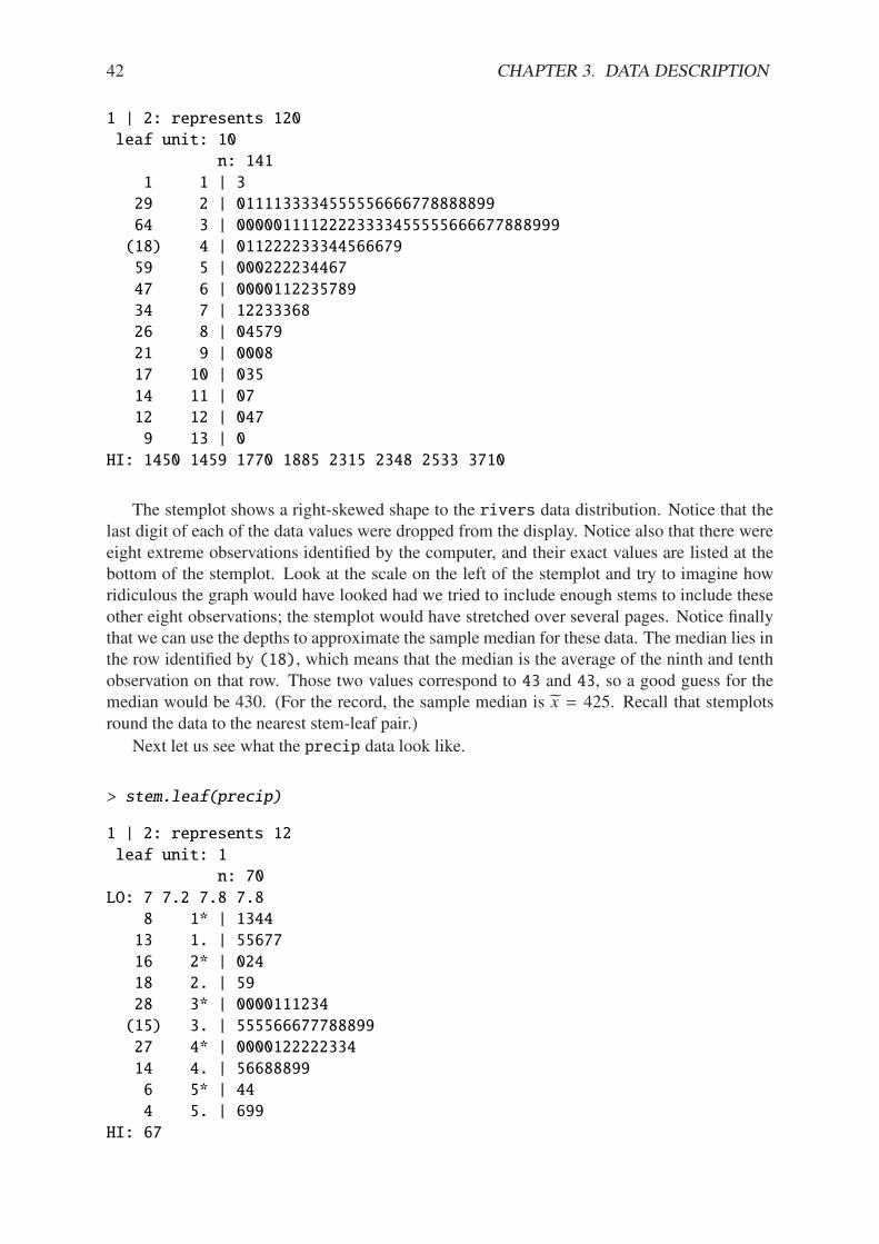
42 CHAPTER 3. DATA DESCRIPTION
1 | 2: represents 120
leaf unit: 10
n: 141
1 1 | 3
29 2 | 0111133334555556666778888899
64 3 | 00000111122223333455555666677888999
(18) 4 | 011222233344566679
59 5 | 000222234467
47 6 | 0000112235789
34 7 | 12233368
26 8 | 04579
21 9 | 0008
17 10 | 035
14 11 | 07
12 12 | 047
9 13 | 0
HI: 1450 1459 1770 1885 2315 2348 2533 3710
The stemplot shows a right-skewed shape to the rivers data distribution. Notice that thelast digit of each of the data values were dropped from the display. Notice also that there wereeight extreme observations identified by the computer, and their exact values are listed at thebottom of the stemplot. Look at the scale on the left of the stemplot and try to imagine howridiculous the graph would have looked had we tried to include enough stems to include theseother eight observations; the stemplot would have stretched over several pages. Notice finallythat we can use the depths to approximate the sample median for these data. The median lies inthe row identified by (18), which means that the median is the average of the ninth and tenthobservation on that row. Those two values correspond to 43 and 43, so a good guess for themedian would be 430. (For the record, the sample median is "x = 425. Recall that stemplotsround the data to the nearest stem-leaf pair.)
Next let us see what the precip data look like.
> stem.leaf(precip)
1 | 2: represents 12
leaf unit: 1
n: 70
LO: 7 7.2 7.8 7.8
8 1* | 1344
13 1. | 55677
16 2* | 024
18 2. | 59
28 3* | 0000111234
(15) 3. | 555566677788899
27 4* | 0000122222334
14 4. | 56688899
6 5* | 44
4 5. | 699
HI: 67
3.4. EXPLORATORY DATA ANALYSIS 43
Here is an example of split stems, with two lines per stem. The final digit of each datumhas been dropped for the display. The data appear to be left skewed with four extreme valuesto the left and one extreme value to the right. The sample median is approximately 37 (it turnsout to be 36.6).
3.4.3 Hinges and the Five Number Summary
Given a data set x1, x2, . . . , xn, the hinges are found by the following method:
• Find the order statistics x(1), x(2), . . . , x(n).
• The lower hinge hL is in position L = ((n + 3)/2) /2, where the symbol (x) denotes thelargest integer less than or equal to x. If the position L is not an integer, then the hingehL is the average of the adjacent order statistics.
• The upper hinge hU is in position n + 1 # L.
Given the hinges, the five number summary (5NS ) is
5NS = (x(1), hL, x, hU , x(n)). (3.4.1)
An advantage of the 5NS is that it reduces a potentially large data set to a shorter list of only fivenumbers, and further, these numbers give insight regarding the shape of the data distributionsimilar to the sample quantiles in Section 3.3.4.
3.4.4 How to do it with R
If the data are stored in a vector x, then you can compute the 5NS with the fivenum function.
3.4.5 Boxplots
A boxplot is essentially a graphical representation of the 5NS . It can be a handy alternative toa stripchart when the sample size is large.
A boxplot is constructed by drawing a box alongside the data axis with sides located atthe upper and lower hinges. A line is drawn parallel to the sides to denote the sample me-dian. Lastly, whiskers are extended from the sides of the box to the maximum and minimumdata values (more precisely, to the most extreme values that are not potential outliers, definedbelow).
Boxplots are good for quick visual summaries of data sets, and the relative positions of thevalues in the 5NS are good at indicating the underlying shape of the data distribution, althoughperhaps not as e!ectively as a histogram. Perhaps the greatest advantage of a boxplot is thatit can help to objectively identify extreme observations in the data set as described in the nextsection.
Boxplots are also good because one can visually assess multiple features of the data setsimultaneously:
Center can be estimated by the sample median, x.
Spread can be judged by the width of the box, hU # hL. We know that this will be close to theIQR, which can be compared to s and the MAD, perhaps after rescaling if appropriate.
44 CHAPTER 3. DATA DESCRIPTION
Shape is indicated by the relative lengths of the whiskers, and the position of the median insidethe box. Boxes with unbalanced whiskers indicate skewness in the direction of the longwhisker. Skewed distributions often have the median tending in the opposite direction ofskewness. Kurtosis can be assessed using the box and whiskers. A wide box with shortwhiskers will tend to be platykurtic, while a skinny box with wide whiskers indicatesleptokurtic distributions.
Extreme observations are identified with open circles (see below).
3.4.6 Outliers
A potential outlier is any observation that falls beyond 1.5 times the width of the box on eitherside, that is, any observation less than hL # 1.5(hU # hL) or greater than hU + 1.5(hU # hL). Asuspected outlier is any observation that falls beyond 3 times the width of the box on eitherside. In R, both potential and suspected outliers (if present) are denoted by open circles; thereis no distinction between the two.
When potential outliers are present, the whiskers of the boxplot are then shortened to extendto the most extreme observation that is not a potential outlier. If an outlier is displayed ina boxplot, the index of the observation may be identified in a subsequent plot in Rcmdr byclicking the Identify outliers with mouse option in the Boxplot dialog.
What do we do about outliers? They merit further investigation. The primary goal is todetermine why the observation is outlying, if possible. If the observation is a typographicalerror, then it should be corrected before continuing. If the observation is from a subject that doesnot belong to the population of interest, then perhaps the datum should be removed. Otherwise,perhaps the value is hinting at some hidden structure to the data.
3.4.7 How to do it with R
The quickest way to visually identify outliers is with a boxplot, described above. Another wayis with the boxplot.stats function.
Example 3.15. The rivers data. We will look for potential outliers in the rivers data.
> boxplot.stats(rivers)$out
[1] 1459 1450 1243 2348 3710 2315 2533 1306 1270 1885 1770
We may change the coef argument to 3 (it is 1.5 by default) to identify suspected outliers.
> boxplot.stats(rivers, coef = 3)$out
[1] 2348 3710 2315 2533 1885
3.4.8 Standardizing variables
It is sometimes useful to compare data sets with each other on a scale that is independent of themeasurement units. Given a set of observed data x1, x2, . . . , xn we get z scores, denoted z1, z2,. . . , zn, by means of the following formula
zi =xi # x
s, i = 1, 2, . . . , n.
3.5. MULTIVARIATE DATA AND DATA FRAMES 45
3.4.9 How to do it with R
The scale function will rescale a numeric vector (or data frame) by subtracting the samplemean from each value (column) and/or by dividing each observation by the sample standarddeviation.
3.5 Multivariate Data and Data Frames
We have had experience with vectors of data, which are long lists of numbers. Typically, eachentry in the vector is a single measurement on a subject or experimental unit in the study. Wesaw in Section 2.3.3 how to form vectors with the c function or the scan function.
However, statistical studies often involve experiments where there are two (or more) mea-surements associated with each subject. We display the measured information in a rectangulararray in which each row corresponds to a subject, and the columns contain the measurementsfor each respective variable. For instance, if one were to measure the height and weight andhair color of each of 11 persons in a research study, the information could be represented witha rectangular array. There would be 11 rows. Each row would have the person’s height in thefirst column and hair color in the second column.
The corresponding objects in R are called data frames, and they can be constructed withthe data.frame function. Each row is an observation, and each column is a variable.
Example 3.16. Suppose we have two vectors x and y and we want to make a data frame out ofthem.
> x <- 5:8
> y <- letters[3:6]
> A <- data.frame(v1 = x, v2 = y)
Notice that x and y are the same length. This is necessary. Also notice that x is a numericvector and y is a character vector. We may choose numeric and character vectors (or evenfactors) for the columns of the data frame, but each column must be of exactly one type. Thatis, we can have a column for height and a column for gender, but we will get an error if wetry to mix function height (numeric) and gender (character or factor) information in the samecolumn.
Indexing of data frames is similar to indexing of vectors. To get the entry in row i andcolumn j do A[i,j]. We can get entire rows and columns by omitting the other index.
> A[3, ]
v1 v2
3 7 e
> A[1, ]
v1 v2
1 5 c
> A[, 2]
[1] c d e f
Levels: c d e f
46 CHAPTER 3. DATA DESCRIPTION
There are several things happening above. Notice that A[3,] gave a data frame (with thesame entries as the third row of A) yet A[1, ] is a numeric vector. A[ ,2] is a factor vectorbecause the default setting for data.frame is stringsAsFactors = TRUE.
Data frames have a names attribute and the names may be extracted with the names func-tion. Once we have the names we may extract given columns by way of the dollar sign.
> names(A)
[1] "v1" "v2"
> A$v1
[1] 5 6 7 8
The above is identical to A[ ,1].
3.5.1 Bivariate Data
• Introduce the sample correlation coe"cient.
• Two-Way Tables. Done with table, or in the R Commander by following Statistics !Contingency Tables ! Two-way Tables. You can also enter and analyze a two-way table.
• Scatterplot: look for linear association and correlation.
* carb ~ optden, data = Formaldehyde
* conc ~ rate, data = Puromycin
* xyplot(accel ~ dist, data = attenu) nonlinear association
* xyplot(eruptions ~ waiting, data = faithful) (linear, two groups)
* xyplot(Petal.Width ~ Petal.Length, data = iris)
* xyplot(pressure ~ temperature, data = pressure) (exponential growth)
* xyplot(weight ~ height, data = women) (strong positive linear)
3.5.2 Multivariate Data
Multivariate Data Display
• Multi-Way Tables. You can do this with table, or in R Commander by following Statis-tics ! Contingency Tables ! Multi-way Tables.
• Scatterplot matrix. used for displaying pairwise scatterplots simultaneously. Again, lookfor linear association and correlation.
• 3D Scatterplot. See Figure 270
• plot(state.region, state.division)
• barplot(table(state.division,state.region), legend.text=TRUE)
3.6. COMPARING POPULATIONS 47
3.6 Comparing Populations
Sometimes we have data from two or more groups (or populations) and we would like to com-pare them and draw conclusions. What we should imagine is
Some issues that we would like to address:
• Comparing centers and spreads: variation within versus between groups
• Comparing clusters and gaps
• Comparing outliers and unusual features
• Comparing shapes.
3.6.1 Numerically
I am thinking here about theStatistics !Numerical Summaries ! Summarize by groups optionor the Statistics ! Summaries !Table of Statistics option.
3.6.2 Graphically
• Boxplots
* Variable width: the width of the drawn boxplots are proportional to$ni, where ni is
the size of the ith group. Why? Because many statistics have variability proportionalto the reciprocal of the square root of the sample size.
* Notches: extend to 1.58·(hU#hL)/$n. The idea is to give roughly a 95% confidence
interval for the di!erence in two medians. See Chapter 10.
• Stripcharts
• Bar Graphs
* plot(xtabs(Freq ~ Admit + Gender, data = UCBAdmissions)) # rescaled barplot
* barplot(xtabs(Freq ~ Admit +Gender, data = UCBAdmissions)) # stacked bar chart
* barplot(xtabs(Freq ~ Admit, data = UCBAdmissions))
* barplot(xtabs(Freq ~ Gender + Admit, data = UCBAdmissions), legend = TRUE,beside = TRUE) # oops, discrimination.
* barplot(xtabs(Freq ~ Admit+Dept, data = UCBAdmissions), legend = TRUE, be-side = TRUE) # di!erent departments have di!erent standards
* barplot(xtabs(Freq ~ Gender+Dept, data = UCBAdmissions), legend = TRUE, be-side = TRUE) # men mostly applied to easy departments, women mostly applied todi"cult departments
* barplot(xtabs(Freq ~ Gender+Dept, data = UCBAdmissions), legend = TRUE, be-side = TRUE)
* barchart(Admit ~ Freq, data = C)
* barchart(Admit ~ Freq|Gender, data = C)
48 CHAPTER 3. DATA DESCRIPTION
* barchart(Admit ~ Freq | Dept, groups = Gender, data = C)
* barchart(Admit ~ Freq | Dept, groups = Gender, data = C, auto.key = TRUE)
• Histograms
* ~ breaks | wool*tension, data = warpbreaks
* ~ weight | feed, data = chickwts
* ~ weight | group, data = PlantGrowth
* ~ count | spray, data = InsectSprays
* ~ len | dose, data = ToothGrowth
* ~ decrease | treatment, data = OrchardSprays (or rowpos or colpos)
• Scatterplots
* xyplot(Petal.Width ~ Petal.Length, data = iris, group = Species)
> library(lattice)
> xyplot()
• Scatterplot matrices
* splom(~ cbind(GNP.deflator,GNP,Unemployed,Armed.Forces,Population,Year,Employed),data = longley)
* splom(~ cbind(pop15,pop75,dpi), data = LifeCycleSavings)
* splom(~ cbind(Murder, Assault, Rape), data = USArrests)
* splom(~ cbind(CONT, INTG, DMNR), data = USJudgeRatings)
* splom(~ cbind(area,peri,shape,perm), data = rock)
* splom(~ cbind(Air.Flow, Water.Temp, Acid.Conc., stack.loss), data = stackloss)
* splom(~ cbind(Fertility,Agriculture,Examination,Education,Catholic,Infant.Mortality),data = swiss)
* splom(~ cbind(Fertility,Agriculture,Examination), data = swiss) (positive and neg-ative)
• Dot charts
* dotchart(USPersonalExpenditure)
* dotchart(t(USPersonalExpenditure))
* dotchart(WorldPhones) (transpose is no good)
* freeny.x is no good, neither is volcano
* dotchart(UCBAdmissions[„1])
* dotplot(Survived ~ Freq | Class, groups = Sex, data = B)
* dotplot(Admit ~ Freq | Dept, groups = Gender, data = C)
3.6. COMPARING POPULATIONS 49
• Mosaic plot
* mosaic(~ Survived + Class + Age + Sex, data = Titanic) (or just mosaic(Titanic))
* mosaic(~ Admit + Dept + Gender, data = UCBAdmissions)
• Quantile-quantile plots: There are two ways to do this. One way is to compare twoindependent samples (of the same size). qqplot(x,y). Another way is to compare thesample quantiles of one variable to the theoretical quantiles of another distribution.
Given two samples {x1, x2, . . . , xn} and {y1, y2, . . . , yn}, we may find the order statistics x(1) "x(2) " · · · " x(n) and y(1) " y(2) " · · · " y(n). Next, plot the n points (x(1), y(1)), (x(2), y(2)),. . . ,(x(n), y(n)).
It is clear that if x(k) = y(k) for all k = 1, 2, . . . , n, then we will have a straight line. It is alsoclear that in the real world, a straight line is NEVER observed, and instead we have a scatterplotthat hopefully had a general linear trend. What do the rules tell us?
• If the y-intercept of the line is greater (less) than zero, then the center of the Y data isgreater (less) than the center of the X data.
• If the slope of the line is greater (less) than one, then the spread of the Y data is greater(less) than the spread of the X data..
3.6.3 Lattice Graphics
The following types of plots are useful when there is one variable of interest and there is afactor in the data set by which the variable is categorized.
It is sometimes nice to set lattice.options(default.theme = "col.whitebg")
Side by side boxplots
> library(lattice)
> bwplot(~weight | feed, data = chickwts)
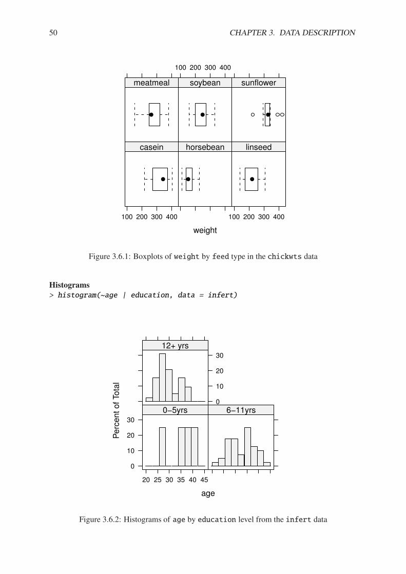
50 CHAPTER 3. DATA DESCRIPTION
weight
100 200 300 400
casein horsebean
100 200 300 400
linseed
meatmeal
100 200 300 400
soybean sunflower
Figure 3.6.1: Boxplots of weight by feed type in the chickwts data
Histograms> histogram(~age | education, data = infert)
age
Perc
ent of To
tal
0
10
20
30
20 25 30 35 40 45
0!5yrs 6!11yrs0
10
20
30
12+ yrs
Figure 3.6.2: Histograms of age by education level from the infert data
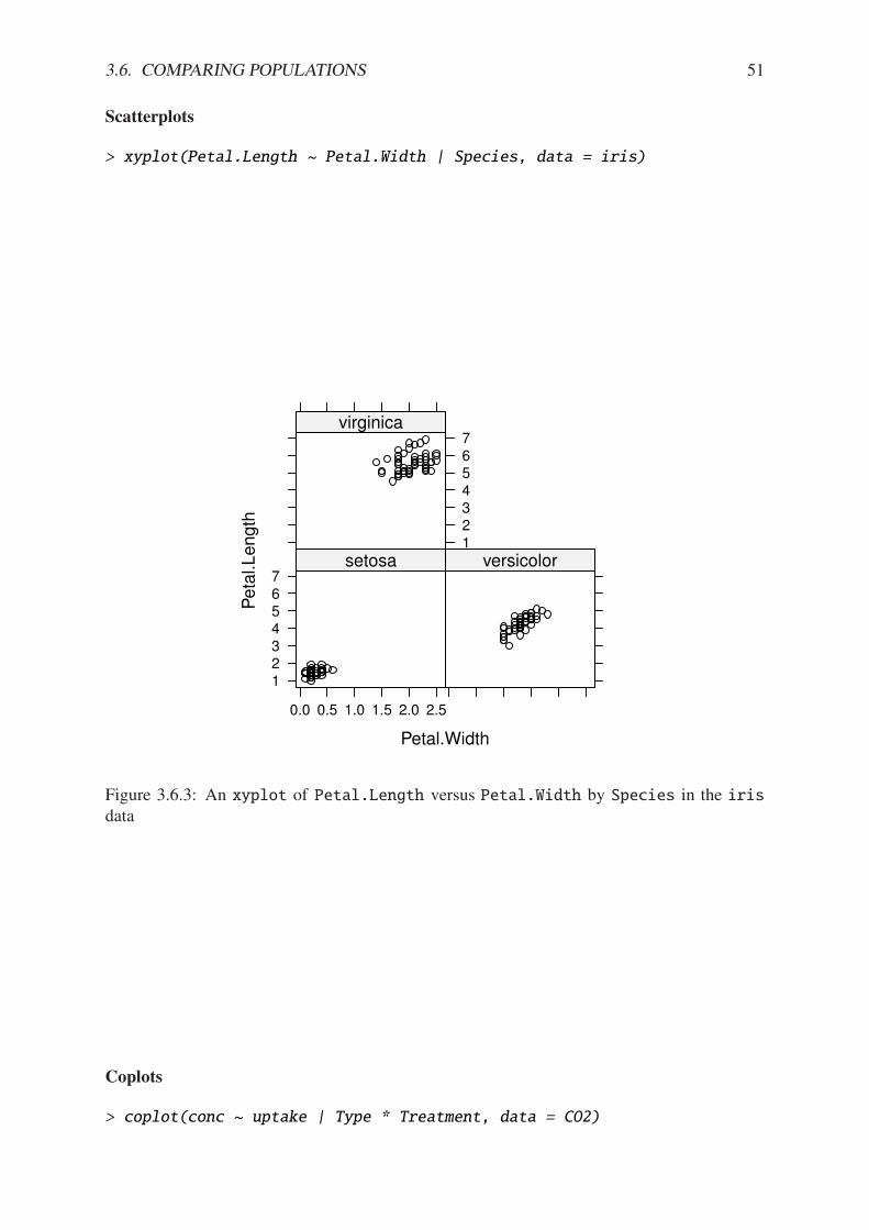
3.6. COMPARING POPULATIONS 51
Scatterplots
> xyplot(Petal.Length ~ Petal.Width | Species, data = iris)
Petal.Width
Peta
l.Length
1234567
0.0 0.5 1.0 1.5 2.0 2.5
setosa versicolor1234567
virginica
Figure 3.6.3: An xyplot of Petal.Length versus Petal.Width by Species in the irisdata
Coplots
> coplot(conc ~ uptake | Type * Treatment, data = CO2)

52 CHAPTER 3. DATA DESCRIPTION
NULL
200
600
1000
10 20 30 40
10 20 30 40
200
600
1000
uptake
conc
Quebec
Mississippi
Given : Type
nonch
illed
chill
ed
Giv
en : T
reatm
ent
Figure 3.6.4: A coplot of conc versus uptake by Type and Treatment in the CO2 data
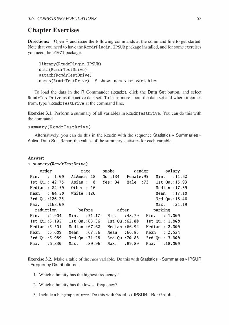
3.6. COMPARING POPULATIONS 53
Chapter Exercises
Directions: Open R and issue the following commands at the command line to get started.Note that you need to have the RcmdrPlugin.IPSUR package installed, and for some exercisesyou need the e1071 package.
library(RcmdrPlugin.IPSUR)
data(RcmdrTestDrive)
attach(RcmdrTestDrive)
names(RcmdrTestDrive) # shows names of variables
To load the data in the R Commander (Rcmdr), click the Data Set button, and selectRcmdrTestDrive as the active data set. To learn more about the data set and where it comesfrom, type ?RcmdrTestDrive at the command line.
Exercise 3.1. Perform a summary of all variables in RcmdrTestDrive. You can do this withthe command
summary(RcmdrTestDrive)
Alternatively, you can do this in the Rcmdr with the sequence Statistics ! Summaries !Active Data Set. Report the values of the summary statistics for each variable.
Answer:
> summary(RcmdrTestDrive)
order race smoke gender salary
Min. : 1.00 AfAmer: 18 No :134 Female:95 Min. :11.62
1st Qu.: 42.75 Asian : 8 Yes: 34 Male :73 1st Qu.:15.93
Median : 84.50 Other : 16 Median :17.59
Mean : 84.50 White :126 Mean :17.10
3rd Qu.:126.25 3rd Qu.:18.46
Max. :168.00 Max. :21.19
reduction before after parking
Min. :4.904 Min. :51.17 Min. :48.79 Min. : 1.000
1st Qu.:5.195 1st Qu.:63.36 1st Qu.:62.80 1st Qu.: 1.000
Median :5.501 Median :67.62 Median :66.94 Median : 2.000
Mean :5.609 Mean :67.36 Mean :66.85 Mean : 2.524
3rd Qu.:5.989 3rd Qu.:71.28 3rd Qu.:70.88 3rd Qu.: 3.000
Max. :6.830 Max. :89.96 Max. :89.89 Max. :18.000
Exercise 3.2. Make a table of the race variable. Do this with Statistics ! Summaries ! IPSUR- Frequency Distributions...
1. Which ethnicity has the highest frequency?
2. Which ethnicity has the lowest frequency?
3. Include a bar graph of race. Do this with Graphs ! IPSUR - Bar Graph...
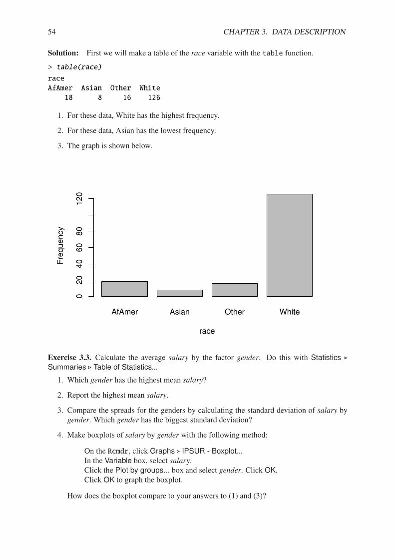
54 CHAPTER 3. DATA DESCRIPTION
Solution: First we will make a table of the race variable with the table function.
> table(race)
race
AfAmer Asian Other White
18 8 16 126
1. For these data, White has the highest frequency.
2. For these data, Asian has the lowest frequency.
3. The graph is shown below.
AfAmer Asian Other White
race
Fre
quency
020
40
60
80
120
Exercise 3.3. Calculate the average salary by the factor gender. Do this with Statistics !Summaries ! Table of Statistics...
1. Which gender has the highest mean salary?
2. Report the highest mean salary.
3. Compare the spreads for the genders by calculating the standard deviation of salary bygender. Which gender has the biggest standard deviation?
4. Make boxplots of salary by gender with the following method:
On the Rcmdr, click Graphs ! IPSUR - Boxplot...In the Variable box, select salary.Click the Plot by groups... box and select gender. Click OK.Click OK to graph the boxplot.
How does the boxplot compare to your answers to (1) and (3)?

3.6. COMPARING POPULATIONS 55
Solution: We can generate a table listing the average salaries by gender with two methods.The first uses tapply:
> x <- tapply(salary, list(gender = gender), mean)
> x
gender
Female Male
16.46353 17.93035
The second method uses the by function:
> by(salary, gender, mean, na.rm = TRUE)
gender: Female
[1] 16.46353
--------------------------------------------------------
gender: Male
[1] 17.93035
Now to answer the questions:
1. Which gender has the highest mean salary?
We can answer this by looking above. For these data, the gender with the highest meansalary is Male.
2. Report the highest mean salary.
Depending on our answer above, we would do something like
mean(salary[gender == Male])
for example. For these data, the highest mean salary is
> x[which(x == max(x))]
Male
17.93035
3. Compare the spreads for the genders by calculating the standard deviation of salary bygender. Which gender has the biggest standard deviation?
> y <- tapply(salary, list(gender = gender), sd)
> y
gender
Female Male
2.122113 1.077183
For these data, the the largest standard deviation is approximately 2.12 which was at-tained by the Female gender.
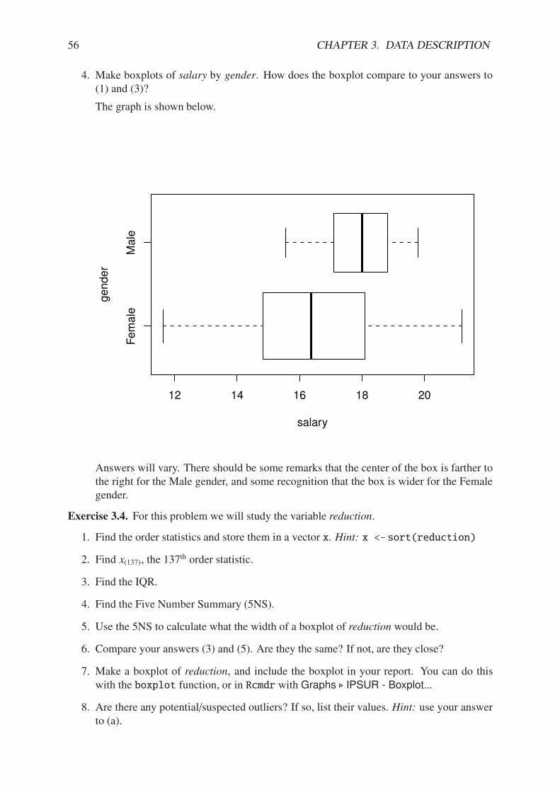
56 CHAPTER 3. DATA DESCRIPTION
4. Make boxplots of salary by gender. How does the boxplot compare to your answers to(1) and (3)?
The graph is shown below.
Fem
ale
Male
12 14 16 18 20
salary
gender
Answers will vary. There should be some remarks that the center of the box is farther tothe right for the Male gender, and some recognition that the box is wider for the Femalegender.
Exercise 3.4. For this problem we will study the variable reduction.
1. Find the order statistics and store them in a vector x. Hint: x <-sort(reduction)
2. Find x(137), the 137th order statistic.
3. Find the IQR.
4. Find the Five Number Summary (5NS).
5. Use the 5NS to calculate what the width of a boxplot of reduction would be.
6. Compare your answers (3) and (5). Are they the same? If not, are they close?
7. Make a boxplot of reduction, and include the boxplot in your report. You can do thiswith the boxplot function, or in Rcmdr with Graphs ! IPSUR - Boxplot...
8. Are there any potential/suspected outliers? If so, list their values. Hint: use your answerto (a).
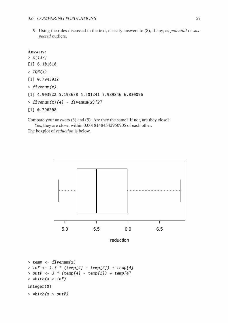
3.6. COMPARING POPULATIONS 57
9. Using the rules discussed in the text, classify answers to (8), if any, as potential or sus-pected outliers.
Answers:> x[137]
[1] 6.101618
> IQR(x)
[1] 0.7943932
> fivenum(x)
[1] 4.903922 5.193638 5.501241 5.989846 6.830096
> fivenum(x)[4] - fivenum(x)[2]
[1] 0.796208
Compare your answers (3) and (5). Are they the same? If not, are they close?Yes, they are close, within 0.00181484542950905 of each other.
The boxplot of reduction is below.
5.0 5.5 6.0 6.5
reduction
> temp <- fivenum(x)
> inF <- 1.5 * (temp[4] - temp[2]) + temp[4]
> outF <- 3 * (temp[4] - temp[2]) + temp[4]
> which(x > inF)
integer(0)
> which(x > outF)
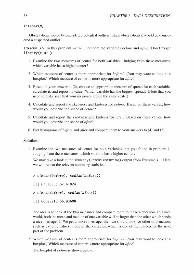
58 CHAPTER 3. DATA DESCRIPTION
integer(0)
Observations would be considered potential outliers, while observation(s) would be consid-ered a suspected outlier.
Exercise 3.5. In this problem we will compare the variables before and after. Don’t forgetlibrary(e1071).
1. Examine the two measures of center for both variables. Judging from these measures,which variable has a higher center?
2. Which measure of center is more appropriate for before? (You may want to look at aboxplot.) Which measure of center is more appropriate for after?
3. Based on your answer to (2), choose an appropriate measure of spread for each variable,calculate it, and report its value. Which variable has the biggest spread? (Note that youneed to make sure that your measures are on the same scale.)
4. Calculate and report the skewness and kurtosis for before. Based on these values, howwould you describe the shape of before?
5. Calculate and report the skewness and kurtosis for after. Based on these values, howwould you describe the shape of after?
6. Plot histograms of before and after and compare them to your answers to (4) and (5).
Solution:
1. Examine the two measures of center for both variables that you found in problem 1.Judging from these measures, which variable has a higher center?
We may take a look at the summary(RcmdrTestDrive) output from Exercise 3.1. Herewe will repeat the relevant summary statistics.
> c(mean(before), median(before))
[1] 67.36338 67.61824
> c(mean(after), median(after))
[1] 66.85215 66.93608
The idea is to look at the two measures and compare them to make a decision. In a niceworld, both the mean and median of one variable will be larger than the other which sendsa nice message. If We get a mixed message, then we should look for other information,such as extreme values in one of the variables, which is one of the reasons for the nextpart of the problem.
2. Which measure of center is more appropriate for before? (You may want to look at aboxplot.) Which measure of center is more appropriate for after?
The boxplot of before is shown below.
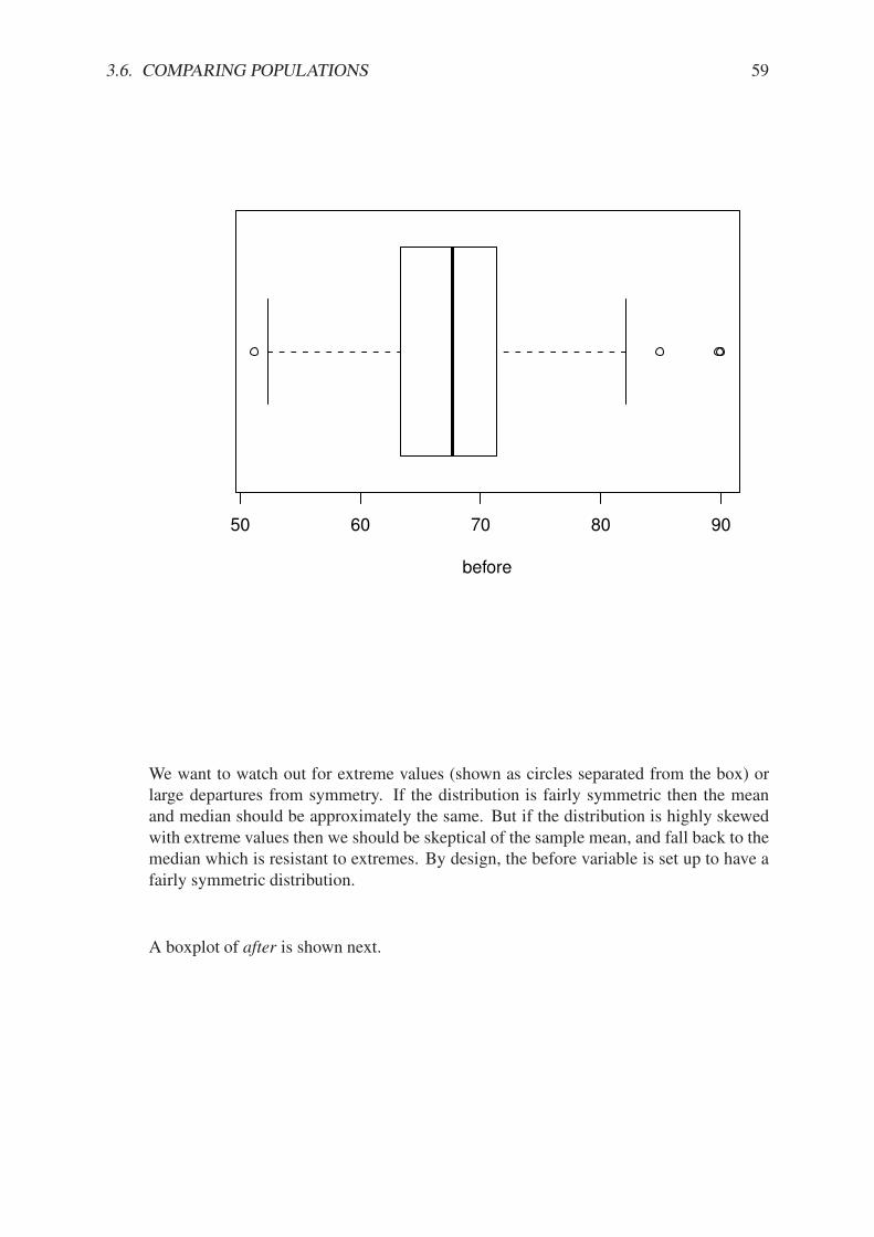
3.6. COMPARING POPULATIONS 59
50 60 70 80 90
before
We want to watch out for extreme values (shown as circles separated from the box) orlarge departures from symmetry. If the distribution is fairly symmetric then the meanand median should be approximately the same. But if the distribution is highly skewedwith extreme values then we should be skeptical of the sample mean, and fall back to themedian which is resistant to extremes. By design, the before variable is set up to have afairly symmetric distribution.
A boxplot of after is shown next.
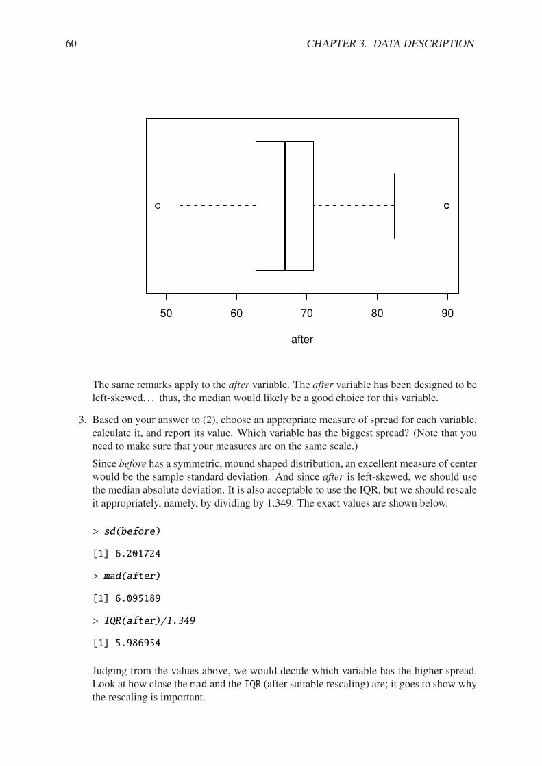
60 CHAPTER 3. DATA DESCRIPTION
50 60 70 80 90
after
The same remarks apply to the after variable. The after variable has been designed to beleft-skewed. . . thus, the median would likely be a good choice for this variable.
3. Based on your answer to (2), choose an appropriate measure of spread for each variable,calculate it, and report its value. Which variable has the biggest spread? (Note that youneed to make sure that your measures are on the same scale.)
Since before has a symmetric, mound shaped distribution, an excellent measure of centerwould be the sample standard deviation. And since after is left-skewed, we should usethe median absolute deviation. It is also acceptable to use the IQR, but we should rescaleit appropriately, namely, by dividing by 1.349. The exact values are shown below.
> sd(before)
[1] 6.201724
> mad(after)
[1] 6.095189
> IQR(after)/1.349
[1] 5.986954
Judging from the values above, we would decide which variable has the higher spread.Look at how close the mad and the IQR (after suitable rescaling) are; it goes to show whythe rescaling is important.
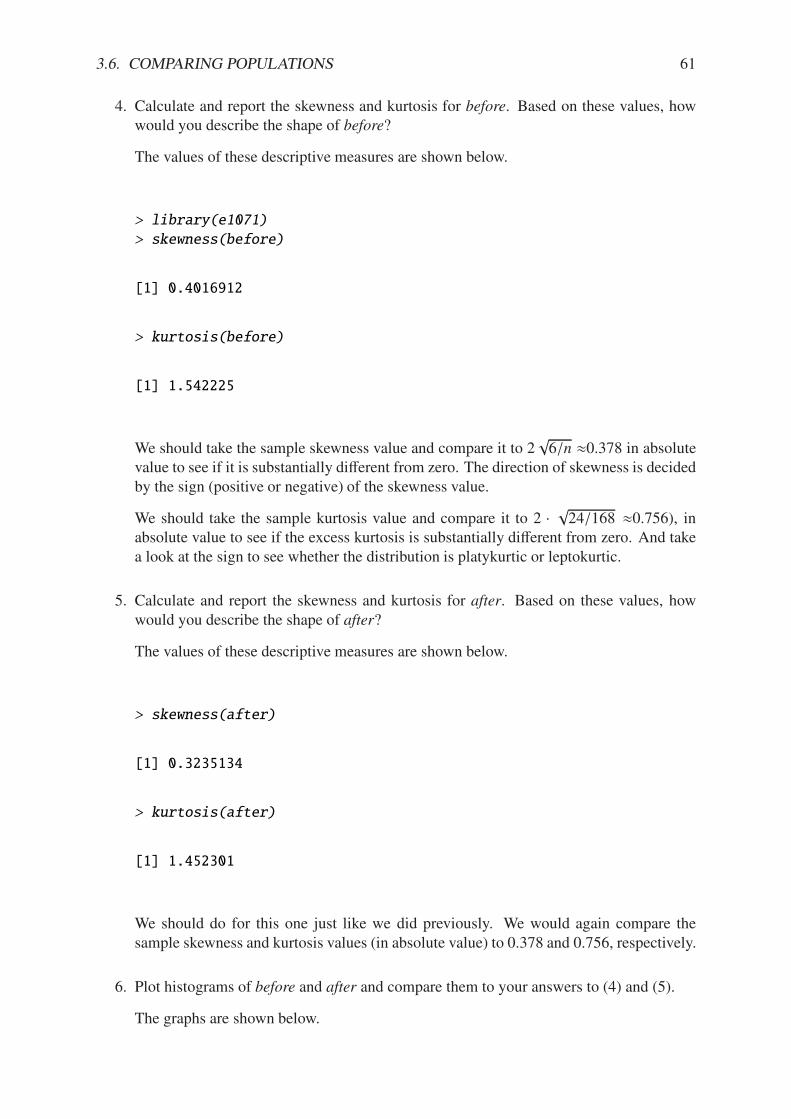
3.6. COMPARING POPULATIONS 61
4. Calculate and report the skewness and kurtosis for before. Based on these values, howwould you describe the shape of before?
The values of these descriptive measures are shown below.
> library(e1071)
> skewness(before)
[1] 0.4016912
> kurtosis(before)
[1] 1.542225
We should take the sample skewness value and compare it to 2$6/n '0.378 in absolute
value to see if it is substantially di!erent from zero. The direction of skewness is decidedby the sign (positive or negative) of the skewness value.
We should take the sample kurtosis value and compare it to 2 ·$24/168 '0.756), in
absolute value to see if the excess kurtosis is substantially di!erent from zero. And takea look at the sign to see whether the distribution is platykurtic or leptokurtic.
5. Calculate and report the skewness and kurtosis for after. Based on these values, howwould you describe the shape of after?
The values of these descriptive measures are shown below.
> skewness(after)
[1] 0.3235134
> kurtosis(after)
[1] 1.452301
We should do for this one just like we did previously. We would again compare thesample skewness and kurtosis values (in absolute value) to 0.378 and 0.756, respectively.
6. Plot histograms of before and after and compare them to your answers to (4) and (5).
The graphs are shown below.
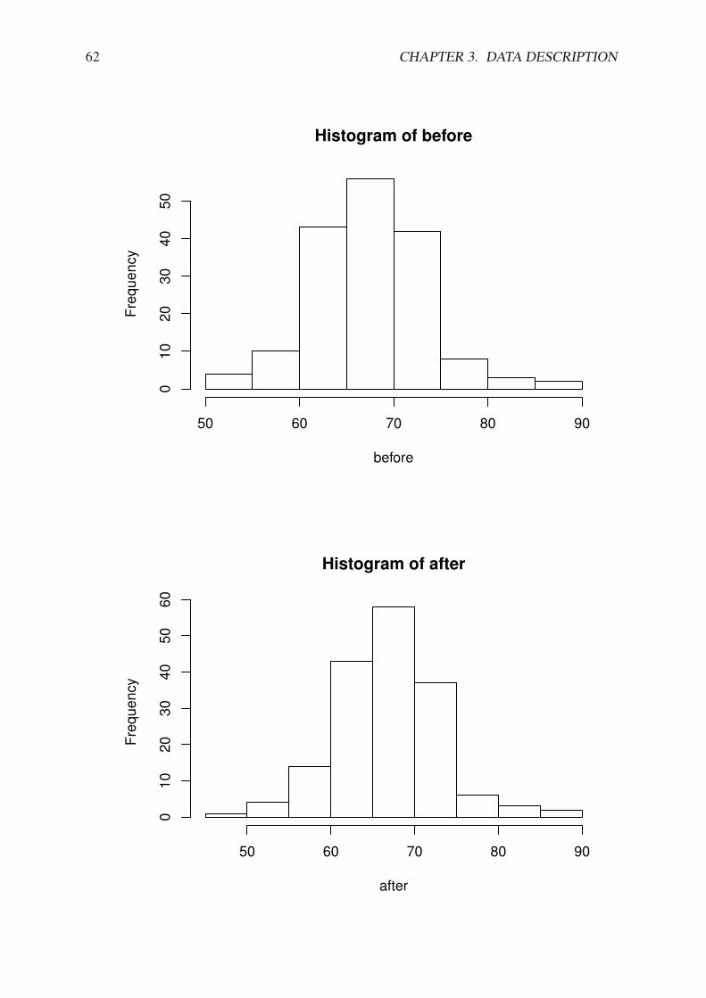
62 CHAPTER 3. DATA DESCRIPTION
Histogram of before
before
Fre
quency
50 60 70 80 90
010
20
30
40
50
Histogram of after
after
Fre
quency
50 60 70 80 90
010
20
30
40
50
60

3.6. COMPARING POPULATIONS 63
Answers will vary. We are looking for visual consistency in the histograms to our state-ments above.
Exercise 3.6. Describe the following data sets just as if you were communicating with analien, but one who has had a statistics class. Mention the salient features (data type, importantproperties, anything special). Support your answers with the appropriate visual displays anddescriptive statistics.
1. Conversion rates of Euro currencies stored in euro.
2. State abbreviations stored in state.abb.

64 CHAPTER 3. DATA DESCRIPTION
Chapter 4
Probability
In this chapter we define the basic terminology associated with probability and derive someof its properties. We discuss three interpretations of probability. We discuss conditional prob-ability and independent events, along with Bayes’ Theorem. We finish the chapter with anintroduction to random variables, which paves the way for the next two chapters.
In this book we distinguish between two types of experiments: deterministic and random.A deterministic experiment is one whose outcome may be predicted with certainty beforehand,such as combining Hydrogen and Oxygen, or adding two numbers such as 2 + 3. A random
experiment is one whose outcome is determined by chance. We posit that the outcome of a ran-dom experiment may not be predicted with certainty beforehand, even in principle. Examplesof random experiments include tossing a coin, rolling a die, and throwing a dart on a board,how many red lights you encounter on the drive home, how many ants traverse a certain patchof sidewalk over a short period, etc.
What do I want them to know?
• that there are multiple interpretations of probability, and the methods used depend some-what on the philosophy chosen
• nuts and bolts of basic probability jargon: sample spaces, events, probability functions,etc.
• how to count
• conditional probability and its relationship with independence
• Bayes’ Rule and how it relates to the subjective view of probability
• what we mean by ’random variables’, and where they come from
4.1 Sample Spaces
For a random experiment E, the set of all possible outcomes of E is called the sample space
and is denoted by the letter S . For the coin-toss experiment, S would be the results “Head”and “Tail”, which we may represent by S = {H, T }. Formally, the performance of a randomexperiment is the unpredictable selection of an outcome in S .
65
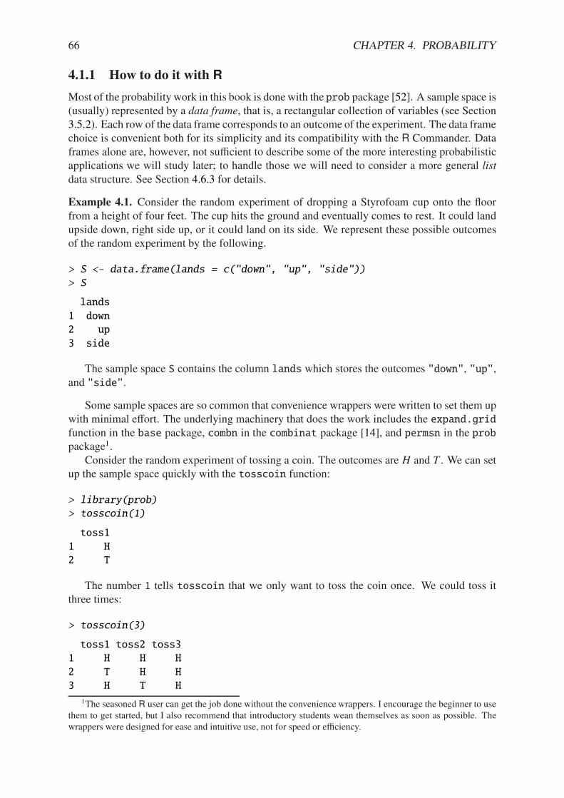
66 CHAPTER 4. PROBABILITY
4.1.1 How to do it with R
Most of the probability work in this book is done with the prob package [52]. A sample space is(usually) represented by a data frame, that is, a rectangular collection of variables (see Section3.5.2). Each row of the data frame corresponds to an outcome of the experiment. The data framechoice is convenient both for its simplicity and its compatibility with the R Commander. Dataframes alone are, however, not su"cient to describe some of the more interesting probabilisticapplications we will study later; to handle those we will need to consider a more general listdata structure. See Section 4.6.3 for details.
Example 4.1. Consider the random experiment of dropping a Styrofoam cup onto the floorfrom a height of four feet. The cup hits the ground and eventually comes to rest. It could landupside down, right side up, or it could land on its side. We represent these possible outcomesof the random experiment by the following.
> S <- data.frame(lands = c("down", "up", "side"))
> S
lands
1 down
2 up
3 side
The sample space S contains the column lands which stores the outcomes "down", "up",and "side".
Some sample spaces are so common that convenience wrappers were written to set them upwith minimal e!ort. The underlying machinery that does the work includes the expand.gridfunction in the base package, combn in the combinat package [14], and permsn in the probpackage1.
Consider the random experiment of tossing a coin. The outcomes are H and T . We can setup the sample space quickly with the tosscoin function:
> library(prob)
> tosscoin(1)
toss1
1 H
2 T
The number 1 tells tosscoin that we only want to toss the coin once. We could toss itthree times:
> tosscoin(3)
toss1 toss2 toss3
1 H H H
2 T H H
3 H T H
1The seasoned R user can get the job done without the convenience wrappers. I encourage the beginner to usethem to get started, but I also recommend that introductory students wean themselves as soon as possible. Thewrappers were designed for ease and intuitive use, not for speed or e"ciency.
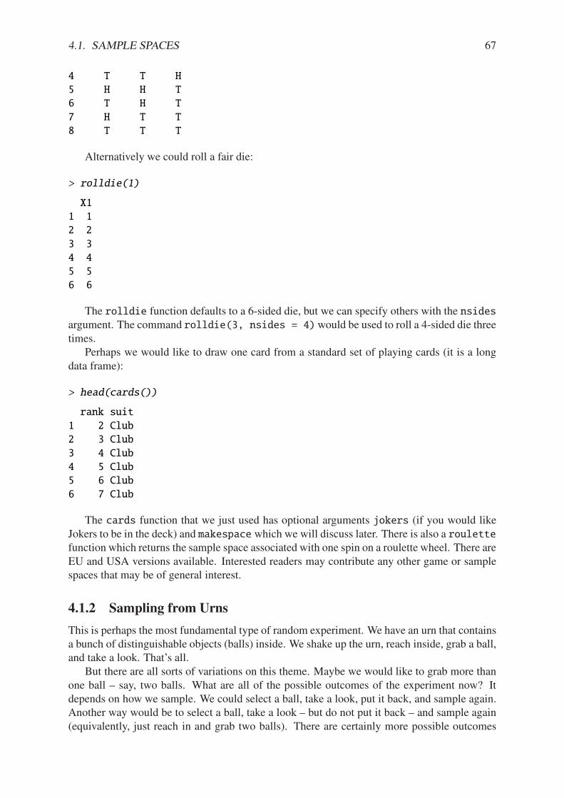
4.1. SAMPLE SPACES 67
4 T T H
5 H H T
6 T H T
7 H T T
8 T T T
Alternatively we could roll a fair die:
> rolldie(1)
X1
1 1
2 2
3 3
4 4
5 5
6 6
The rolldie function defaults to a 6-sided die, but we can specify others with the nsidesargument. The command rolldie(3, nsides = 4)would be used to roll a 4-sided die threetimes.
Perhaps we would like to draw one card from a standard set of playing cards (it is a longdata frame):
> head(cards())
rank suit
1 2 Club
2 3 Club
3 4 Club
4 5 Club
5 6 Club
6 7 Club
The cards function that we just used has optional arguments jokers (if you would likeJokers to be in the deck) and makespace which we will discuss later. There is also a roulettefunction which returns the sample space associated with one spin on a roulette wheel. There areEU and USA versions available. Interested readers may contribute any other game or samplespaces that may be of general interest.
4.1.2 Sampling from Urns
This is perhaps the most fundamental type of random experiment. We have an urn that containsa bunch of distinguishable objects (balls) inside. We shake up the urn, reach inside, grab a ball,and take a look. That’s all.
But there are all sorts of variations on this theme. Maybe we would like to grab more thanone ball – say, two balls. What are all of the possible outcomes of the experiment now? Itdepends on how we sample. We could select a ball, take a look, put it back, and sample again.Another way would be to select a ball, take a look – but do not put it back – and sample again(equivalently, just reach in and grab two balls). There are certainly more possible outcomes
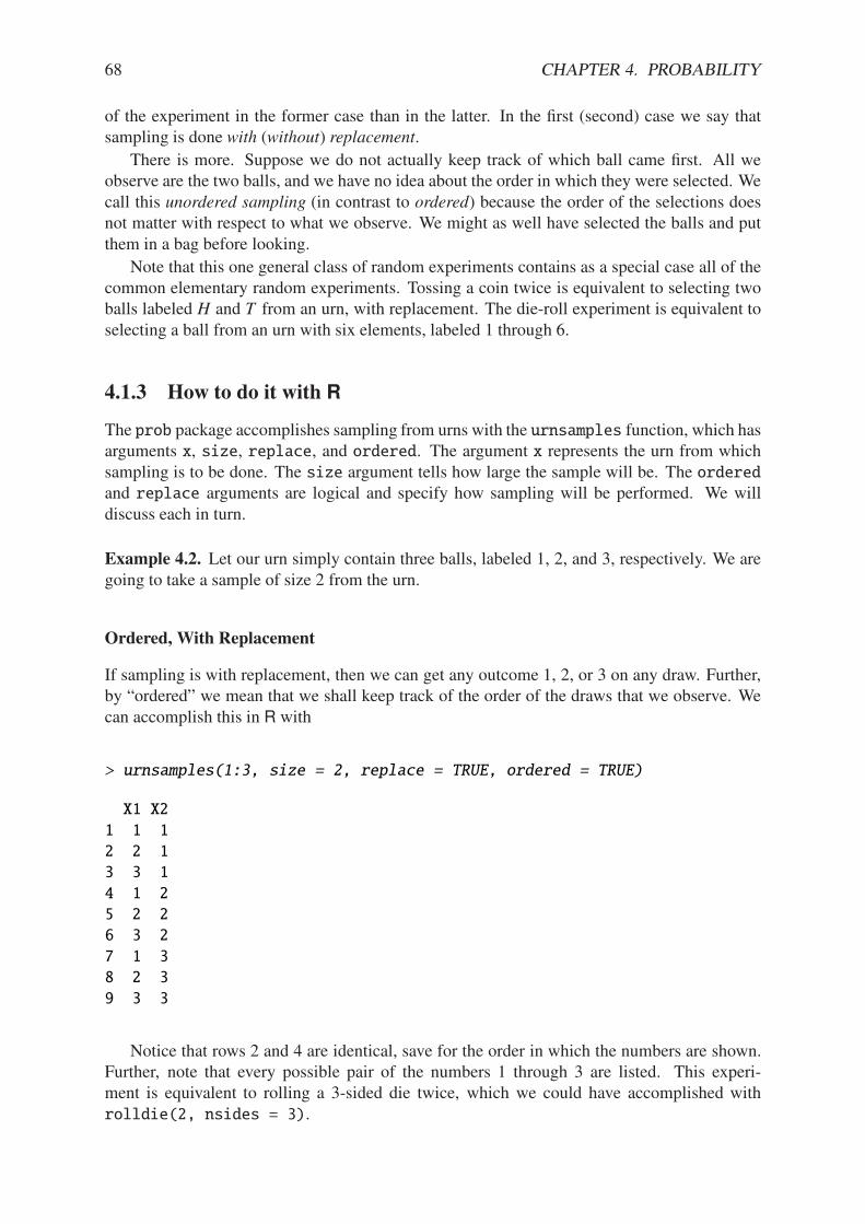
68 CHAPTER 4. PROBABILITY
of the experiment in the former case than in the latter. In the first (second) case we say thatsampling is done with (without) replacement.
There is more. Suppose we do not actually keep track of which ball came first. All weobserve are the two balls, and we have no idea about the order in which they were selected. Wecall this unordered sampling (in contrast to ordered) because the order of the selections doesnot matter with respect to what we observe. We might as well have selected the balls and putthem in a bag before looking.
Note that this one general class of random experiments contains as a special case all of thecommon elementary random experiments. Tossing a coin twice is equivalent to selecting twoballs labeled H and T from an urn, with replacement. The die-roll experiment is equivalent toselecting a ball from an urn with six elements, labeled 1 through 6.
4.1.3 How to do it with R
The prob package accomplishes sampling from urns with the urnsamples function, which hasarguments x, size, replace, and ordered. The argument x represents the urn from whichsampling is to be done. The size argument tells how large the sample will be. The orderedand replace arguments are logical and specify how sampling will be performed. We willdiscuss each in turn.
Example 4.2. Let our urn simply contain three balls, labeled 1, 2, and 3, respectively. We aregoing to take a sample of size 2 from the urn.
Ordered, With Replacement
If sampling is with replacement, then we can get any outcome 1, 2, or 3 on any draw. Further,by “ordered” we mean that we shall keep track of the order of the draws that we observe. Wecan accomplish this in R with
> urnsamples(1:3, size = 2, replace = TRUE, ordered = TRUE)
X1 X2
1 1 1
2 2 1
3 3 1
4 1 2
5 2 2
6 3 2
7 1 3
8 2 3
9 3 3
Notice that rows 2 and 4 are identical, save for the order in which the numbers are shown.Further, note that every possible pair of the numbers 1 through 3 are listed. This experi-ment is equivalent to rolling a 3-sided die twice, which we could have accomplished withrolldie(2, nsides = 3).
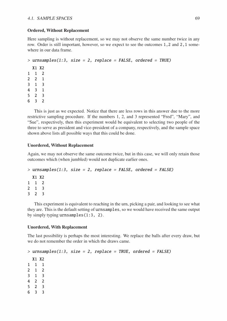
4.1. SAMPLE SPACES 69
Ordered, Without Replacement
Here sampling is without replacement, so we may not observe the same number twice in anyrow. Order is still important, however, so we expect to see the outcomes 1,2 and 2,1 some-where in our data frame.
> urnsamples(1:3, size = 2, replace = FALSE, ordered = TRUE)
X1 X2
1 1 2
2 2 1
3 1 3
4 3 1
5 2 3
6 3 2
This is just as we expected. Notice that there are less rows in this answer due to the morerestrictive sampling procedure. If the numbers 1, 2, and 3 represented “Fred”, “Mary”, and“Sue”, respectively, then this experiment would be equivalent to selecting two people of thethree to serve as president and vice-president of a company, respectively, and the sample spaceshown above lists all possible ways that this could be done.
Unordered, Without Replacement
Again, we may not observe the same outcome twice, but in this case, we will only retain thoseoutcomes which (when jumbled) would not duplicate earlier ones.
> urnsamples(1:3, size = 2, replace = FALSE, ordered = FALSE)
X1 X2
1 1 2
2 1 3
3 2 3
This experiment is equivalent to reaching in the urn, picking a pair, and looking to see whatthey are. This is the default setting of urnsamples, so we would have received the same outputby simply typing urnsamples(1:3, 2).
Unordered, With Replacement
The last possibility is perhaps the most interesting. We replace the balls after every draw, butwe do not remember the order in which the draws came.
> urnsamples(1:3, size = 2, replace = TRUE, ordered = FALSE)
X1 X2
1 1 1
2 1 2
3 1 3
4 2 2
5 2 3
6 3 3
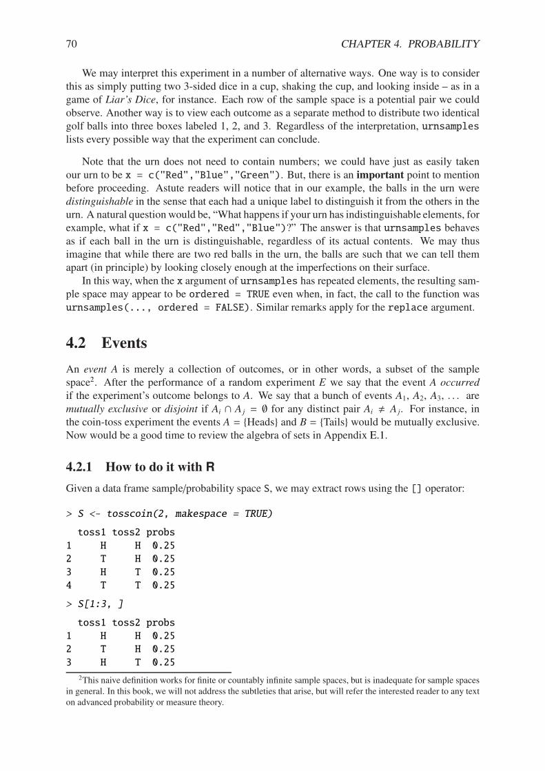
70 CHAPTER 4. PROBABILITY
We may interpret this experiment in a number of alternative ways. One way is to considerthis as simply putting two 3-sided dice in a cup, shaking the cup, and looking inside – as in agame of Liar’s Dice, for instance. Each row of the sample space is a potential pair we couldobserve. Another way is to view each outcome as a separate method to distribute two identicalgolf balls into three boxes labeled 1, 2, and 3. Regardless of the interpretation, urnsampleslists every possible way that the experiment can conclude.
Note that the urn does not need to contain numbers; we could have just as easily takenour urn to be x = c("Red","Blue","Green"). But, there is an important point to mentionbefore proceeding. Astute readers will notice that in our example, the balls in the urn weredistinguishable in the sense that each had a unique label to distinguish it from the others in theurn. A natural question would be, “What happens if your urn has indistinguishable elements, forexample, what if x = c("Red","Red","Blue")?” The answer is that urnsamples behavesas if each ball in the urn is distinguishable, regardless of its actual contents. We may thusimagine that while there are two red balls in the urn, the balls are such that we can tell themapart (in principle) by looking closely enough at the imperfections on their surface.
In this way, when the x argument of urnsamples has repeated elements, the resulting sam-ple space may appear to be ordered = TRUE even when, in fact, the call to the function wasurnsamples(..., ordered = FALSE). Similar remarks apply for the replace argument.
4.2 Events
An event A is merely a collection of outcomes, or in other words, a subset of the samplespace2. After the performance of a random experiment E we say that the event A occurred
if the experiment’s outcome belongs to A. We say that a bunch of events A1, A2, A3, . . . aremutually exclusive or disjoint if Ai + Aj = , for any distinct pair Ai ! Aj. For instance, inthe coin-toss experiment the events A = {Heads} and B = {Tails} would be mutually exclusive.Now would be a good time to review the algebra of sets in Appendix E.1.
4.2.1 How to do it with R
Given a data frame sample/probability space S, we may extract rows using the [] operator:
> S <- tosscoin(2, makespace = TRUE)
toss1 toss2 probs
1 H H 0.25
2 T H 0.25
3 H T 0.25
4 T T 0.25
> S[1:3, ]
toss1 toss2 probs
1 H H 0.25
2 T H 0.25
3 H T 0.25
2This naive definition works for finite or countably infinite sample spaces, but is inadequate for sample spacesin general. In this book, we will not address the subtleties that arise, but will refer the interested reader to any texton advanced probability or measure theory.
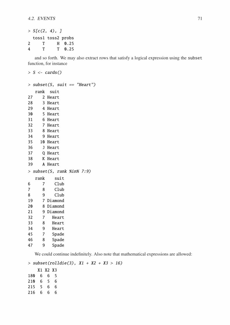
4.2. EVENTS 71
> S[c(2, 4), ]
toss1 toss2 probs
2 T H 0.25
4 T T 0.25
and so forth. We may also extract rows that satisfy a logical expression using the subsetfunction, for instance
> S <- cards()
> subset(S, suit == "Heart")
rank suit
27 2 Heart
28 3 Heart
29 4 Heart
30 5 Heart
31 6 Heart
32 7 Heart
33 8 Heart
34 9 Heart
35 10 Heart
36 J Heart
37 Q Heart
38 K Heart
39 A Heart
> subset(S, rank %in% 7:9)
rank suit
6 7 Club
7 8 Club
8 9 Club
19 7 Diamond
20 8 Diamond
21 9 Diamond
32 7 Heart
33 8 Heart
34 9 Heart
45 7 Spade
46 8 Spade
47 9 Spade
We could continue indefinitely. Also note that mathematical expressions are allowed:
> subset(rolldie(3), X1 + X2 + X3 > 16)
X1 X2 X3
180 6 6 5
210 6 5 6
215 5 6 6
216 6 6 6
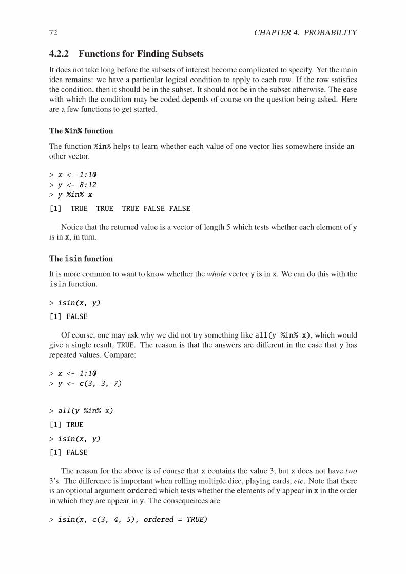
72 CHAPTER 4. PROBABILITY
4.2.2 Functions for Finding Subsets
It does not take long before the subsets of interest become complicated to specify. Yet the mainidea remains: we have a particular logical condition to apply to each row. If the row satisfiesthe condition, then it should be in the subset. It should not be in the subset otherwise. The easewith which the condition may be coded depends of course on the question being asked. Hereare a few functions to get started.
The %in% function
The function %in% helps to learn whether each value of one vector lies somewhere inside an-other vector.
> x <- 1:10
> y <- 8:12
> y %in% x
[1] TRUE TRUE TRUE FALSE FALSE
Notice that the returned value is a vector of length 5 which tests whether each element of yis in x, in turn.
The isin function
It is more common to want to know whether the whole vector y is in x. We can do this with theisin function.
> isin(x, y)
[1] FALSE
Of course, one may ask why we did not try something like all(y %in% x), which wouldgive a single result, TRUE. The reason is that the answers are di!erent in the case that y hasrepeated values. Compare:
> x <- 1:10
> y <- c(3, 3, 7)
> all(y %in% x)
[1] TRUE
> isin(x, y)
[1] FALSE
The reason for the above is of course that x contains the value 3, but x does not have two3’s. The di!erence is important when rolling multiple dice, playing cards, etc. Note that thereis an optional argument ordered which tests whether the elements of y appear in x in the orderin which they are appear in y. The consequences are
> isin(x, c(3, 4, 5), ordered = TRUE)
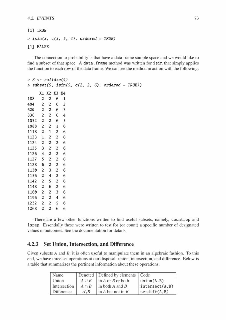
4.2. EVENTS 73
[1] TRUE
> isin(x, c(3, 5, 4), ordered = TRUE)
[1] FALSE
The connection to probability is that have a data frame sample space and we would like tofind a subset of that space. A data.frame method was written for isin that simply appliesthe function to each row of the data frame. We can see the method in action with the following:
> S <- rolldie(4)
> subset(S, isin(S, c(2, 2, 6), ordered = TRUE))
X1 X2 X3 X4
188 2 2 6 1
404 2 2 6 2
620 2 2 6 3
836 2 2 6 4
1052 2 2 6 5
1088 2 2 1 6
1118 2 1 2 6
1123 1 2 2 6
1124 2 2 2 6
1125 3 2 2 6
1126 4 2 2 6
1127 5 2 2 6
1128 6 2 2 6
1130 2 3 2 6
1136 2 4 2 6
1142 2 5 2 6
1148 2 6 2 6
1160 2 2 3 6
1196 2 2 4 6
1232 2 2 5 6
1268 2 2 6 6
There are a few other functions written to find useful subsets, namely, countrep andisrep. Essentially these were written to test for (or count) a specific number of designatedvalues in outcomes. See the documentation for details.
4.2.3 Set Union, Intersection, and Di!erence
Given subsets A and B, it is often useful to manipulate them in an algebraic fashion. To thisend, we have three set operations at our disposal: union, intersection, and di!erence. Below isa table that summarizes the pertinent information about these operations.
Name Denoted Defined by elements CodeUnion A - B in A or B or both union(A,B)
Intersection A + B in both A and B intersect(A,B)
Di!erence A\B in A but not in B setdiff(A,B)
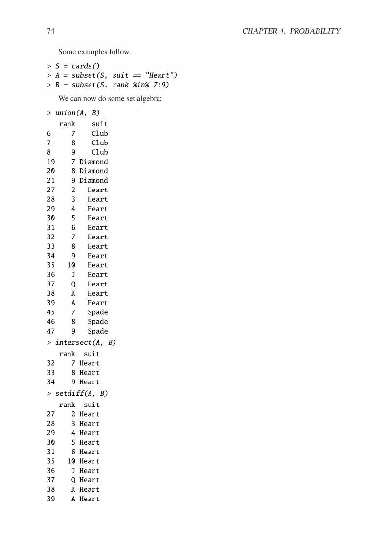
74 CHAPTER 4. PROBABILITY
Some examples follow.
> S = cards()
> A = subset(S, suit == "Heart")
> B = subset(S, rank %in% 7:9)
We can now do some set algebra:
> union(A, B)
rank suit
6 7 Club
7 8 Club
8 9 Club
19 7 Diamond
20 8 Diamond
21 9 Diamond
27 2 Heart
28 3 Heart
29 4 Heart
30 5 Heart
31 6 Heart
32 7 Heart
33 8 Heart
34 9 Heart
35 10 Heart
36 J Heart
37 Q Heart
38 K Heart
39 A Heart
45 7 Spade
46 8 Spade
47 9 Spade
> intersect(A, B)
rank suit
32 7 Heart
33 8 Heart
34 9 Heart
> setdiff(A, B)
rank suit
27 2 Heart
28 3 Heart
29 4 Heart
30 5 Heart
31 6 Heart
35 10 Heart
36 J Heart
37 Q Heart
38 K Heart
39 A Heart
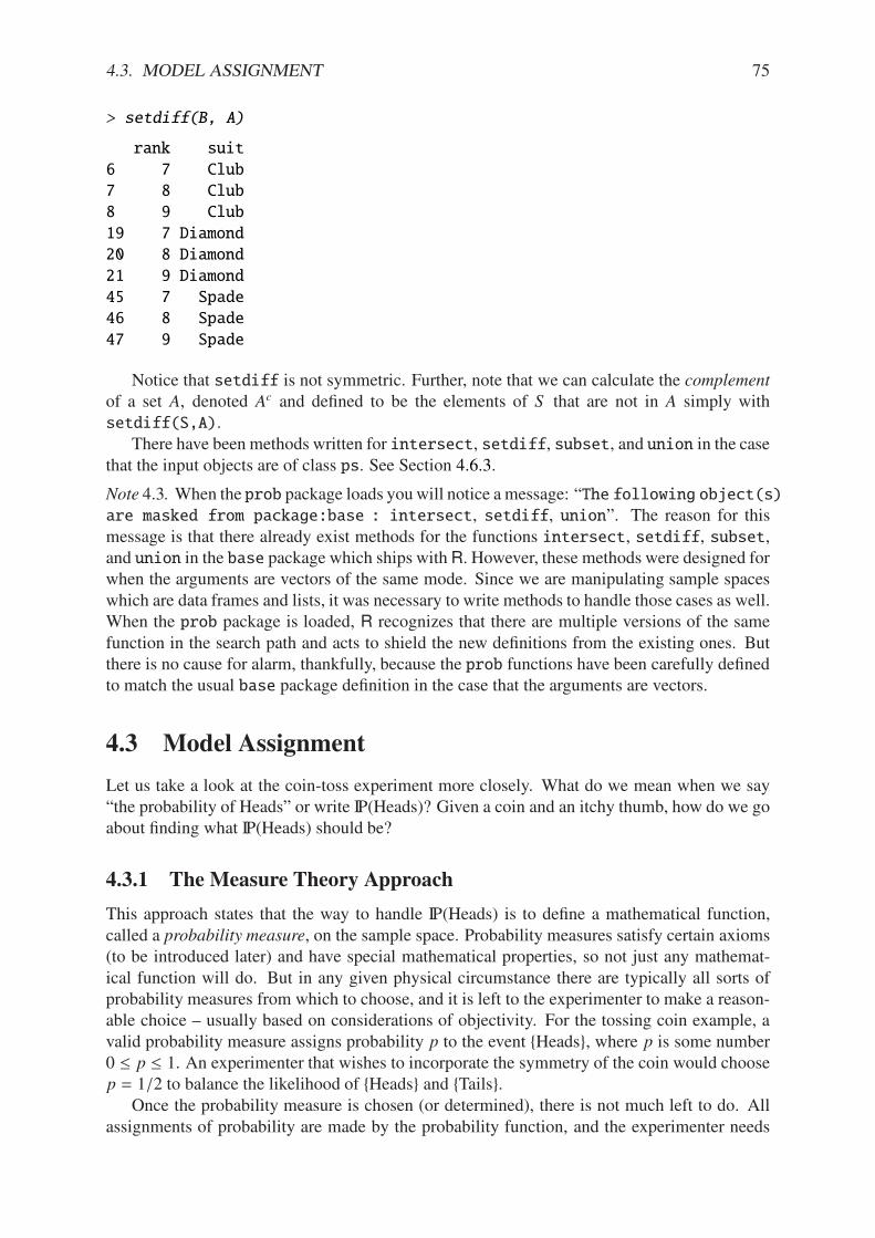
4.3. MODEL ASSIGNMENT 75
> setdiff(B, A)
rank suit
6 7 Club
7 8 Club
8 9 Club
19 7 Diamond
20 8 Diamond
21 9 Diamond
45 7 Spade
46 8 Spade
47 9 Spade
Notice that setdiff is not symmetric. Further, note that we can calculate the complementof a set A, denoted Ac and defined to be the elements of S that are not in A simply withsetdiff(S,A).
There have been methods written for intersect, setdiff, subset, and union in the casethat the input objects are of class ps. See Section 4.6.3.
Note 4.3. When the prob package loads you will notice a message: “The following object(s)are masked from package:base : intersect, setdiff, union”. The reason for thismessage is that there already exist methods for the functions intersect, setdiff, subset,and union in the base package which ships with R. However, these methods were designed forwhen the arguments are vectors of the same mode. Since we are manipulating sample spaceswhich are data frames and lists, it was necessary to write methods to handle those cases as well.When the prob package is loaded, R recognizes that there are multiple versions of the samefunction in the search path and acts to shield the new definitions from the existing ones. Butthere is no cause for alarm, thankfully, because the prob functions have been carefully definedto match the usual base package definition in the case that the arguments are vectors.
4.3 Model Assignment
Let us take a look at the coin-toss experiment more closely. What do we mean when we say“the probability of Heads” or write IP(Heads)? Given a coin and an itchy thumb, how do we goabout finding what IP(Heads) should be?
4.3.1 The Measure Theory Approach
This approach states that the way to handle IP(Heads) is to define a mathematical function,called a probability measure, on the sample space. Probability measures satisfy certain axioms(to be introduced later) and have special mathematical properties, so not just any mathemat-ical function will do. But in any given physical circumstance there are typically all sorts ofprobability measures from which to choose, and it is left to the experimenter to make a reason-able choice – usually based on considerations of objectivity. For the tossing coin example, avalid probability measure assigns probability p to the event {Heads}, where p is some number0 " p " 1. An experimenter that wishes to incorporate the symmetry of the coin would choosep = 1/2 to balance the likelihood of {Heads} and {Tails}.
Once the probability measure is chosen (or determined), there is not much left to do. Allassignments of probability are made by the probability function, and the experimenter needs
76 CHAPTER 4. PROBABILITY
only to plug the event {Heads} into to the probability function to find IP(Heads). In this way,the probability of an event is simply a calculated value, nothing more, nothing less. Of coursethis is not the whole story; there are many theorems and consequences associated with thisapproach that will keep us occupied for the remainder of this book. The approach is calledmeasure theory because the measure (probability) of a set (event) is associated with how big itis (how likely it is to occur).
The measure theory approach is well suited for situations where there is symmetry to theexperiment, such as flipping a balanced coin or spinning an arrow around a circle with well-defined pie slices. It is also handy because of its mathematical simplicity, elegance, and flexibil-ity. There are literally volumes of information that one can prove about probability measures,and the cold rules of mathematics allow us to analyze intricate probabilistic problems withvigor.
The large degree of flexibility is also a disadvantage, however. When symmetry fails it isnot always obvious what an “objective” choice of probability measure should be; for instance,what probability should we assign to {Heads} if we spin the coin rather than flip it? (It isnot 1/2.) Furthermore, the mathematical rules are restrictive when we wish to incorporatesubjective knowledge into the model, knowledge which changes over time and depends onthe experimenter, such as personal knowledge about the properties of the specific coin beingflipped, or of the person doing the flipping.
The mathematician who revolutionized this way to do probability theory was Andrey Kol-mogorov, who published a landmark monograph in 1933. See
http://www-history.mcs.st-andrews.ac.uk/Mathematicians/Kolmogorov.html
for more information.
4.3.2 Relative Frequency Approach
This approach states that the way to determine IP(Heads) is to flip the coin repeatedly, in exactlythe same way each time. Keep a tally of the number of flips and the number of Heads observed.Then a good approximation to IP(Heads) will be
IP(Heads) 'number of observed Heads
total number of flips. (4.3.1)
The mathematical underpinning of this approach is the celebrated Law of Large Numbers,which may be loosely described as follows. Let E be a random experiment in which the eventA either does or does not occur. Perform the experiment repeatedly, in an identical manner, insuch a way that the successive experiments do not influence each other. After each experiment,keep a running tally of whether or not the event A occurred. Let S n count the number of timesthat A occurred in the n experiments. Then the law of large numbers says that
S n
n. IP(A) as n . &. (4.3.2)
As the reasoning goes, to learn about the probability of an event A we need only repeat therandom experiment to get a reasonable estimate of the probability’s value, and if we are notsatisfied with our estimate then we may simply repeat the experiment more times all the whileconfident that with more and more experiments our estimate will stabilize to the true value.
The frequentist approach is good because it is relatively light on assumptions and does notworry about symmetry or claims of objectivity like the measure-theoretic approach does. It is
4.3. MODEL ASSIGNMENT 77
perfect for the spinning coin experiment. One drawback to the method is that one can neverknow the exact value of a probability, only a long-run approximation. It also does not workwell with experiments that can not be repeated indefinitely, say, the probability that it will raintoday, the chances that you get will get an A in your Statistics class, or the probability that theworld is destroyed by nuclear war.
This approach was espoused by Richard von Mises in the early twentieth century, and someof his main ideas were incorporated into the measure theory approach. See
http://www-history.mcs.st-andrews.ac.uk/Biographies/Mises.html
for more.
4.3.3 The Subjective Approach
The subjective approach interprets probability as the experimenter’s degree of belief that theevent will occur. The estimate of the probability of an event is based on the totality of the indi-vidual’s knowledge at the time. As new information becomes available, the estimate is modifiedaccordingly to best reflect his/her current knowledge. The method by which the probabilitiesare updated is commonly done with Bayes’ Rule, discussed in Section 4.8.
So for the coin toss example, a person may have IP(Heads) = 1/2 in the absence of addi-tional information. But perhaps the observer knows additional information about the coin or thethrower that would shift the probability in a certain direction. For instance, parlor magiciansmay be trained to be quite skilled at tossing coins, and some are so skilled that they may toss afair coin and get nothing but Heads, indefinitely. I have seen this. It was similarly claimed inBringing Down the House [65] that MIT students were accomplished enough with cards to beable to cut a deck to the same location, every single time. In such cases, one clearly should usethe additional information to assign IP(Heads) away from the symmetry value of 1/2.
This approach works well in situations that cannot be repeated indefinitely, for example, toassign your probability that you will get an A in this class, the chances of a devastating nuclearwar, or the likelihood that a cure for the common cold will be discovered.
The roots of subjective probability reach back a long time. See
http://en.wikipedia.org/wiki/Subjective_probability
for a short discussion and links to references about the subjective approach.
4.3.4 Equally Likely Model (ELM)
We have seen several approaches to the assignment of a probability model to a given randomexperiment and they are very di!erent in their underlying interpretation. But they all cross pathswhen it comes to the equally likely model which assigns equal probability to all elementaryoutcomes of the experiment.
The ELM appears in the measure theory approach when the experiment boasts symmetryof some kind. If symmetry guarantees that all outcomes have equal “size”, and if outcomeswith equal “size” should get the same probability, then the ELM is a logical objective choicefor the experimenter. Consider the balanced 6-sided die, the fair coin, or the dart board withequal-sized wedges.
The ELM appears in the subjective approach when the experimenter resorts to indi!er-ence or ignorance with respect to his/her knowledge of the outcome of the experiment. If the
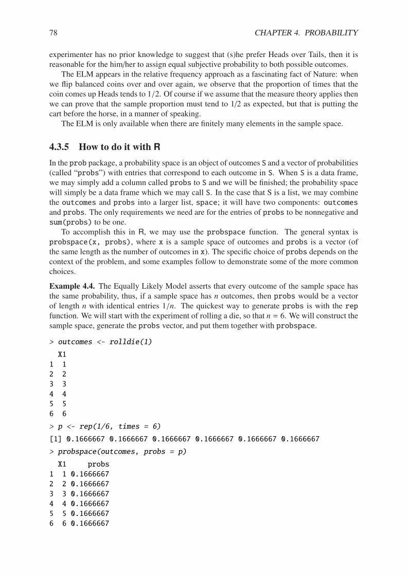
78 CHAPTER 4. PROBABILITY
experimenter has no prior knowledge to suggest that (s)he prefer Heads over Tails, then it isreasonable for the him/her to assign equal subjective probability to both possible outcomes.
The ELM appears in the relative frequency approach as a fascinating fact of Nature: whenwe flip balanced coins over and over again, we observe that the proportion of times that thecoin comes up Heads tends to 1/2. Of course if we assume that the measure theory applies thenwe can prove that the sample proportion must tend to 1/2 as expected, but that is putting thecart before the horse, in a manner of speaking.
The ELM is only available when there are finitely many elements in the sample space.
4.3.5 How to do it with R
In the prob package, a probability space is an object of outcomes S and a vector of probabilities(called “probs”) with entries that correspond to each outcome in S. When S is a data frame,we may simply add a column called probs to S and we will be finished; the probability spacewill simply be a data frame which we may call S. In the case that S is a list, we may combinethe outcomes and probs into a larger list, space; it will have two components: outcomesand probs. The only requirements we need are for the entries of probs to be nonnegative andsum(probs) to be one.
To accomplish this in R, we may use the probspace function. The general syntax isprobspace(x, probs), where x is a sample space of outcomes and probs is a vector (ofthe same length as the number of outcomes in x). The specific choice of probs depends on thecontext of the problem, and some examples follow to demonstrate some of the more commonchoices.
Example 4.4. The Equally Likely Model asserts that every outcome of the sample space hasthe same probability, thus, if a sample space has n outcomes, then probs would be a vectorof length n with identical entries 1/n. The quickest way to generate probs is with the repfunction. We will start with the experiment of rolling a die, so that n = 6. We will construct thesample space, generate the probs vector, and put them together with probspace.
> outcomes <- rolldie(1)
X1
1 1
2 2
3 3
4 4
5 5
6 6
> p <- rep(1/6, times = 6)
[1] 0.1666667 0.1666667 0.1666667 0.1666667 0.1666667 0.1666667
> probspace(outcomes, probs = p)
X1 probs
1 1 0.1666667
2 2 0.1666667
3 3 0.1666667
4 4 0.1666667
5 5 0.1666667
6 6 0.1666667
4.3. MODEL ASSIGNMENT 79
The probspace function is designed to save us some time in many of the most commonsituations. For example, due to the especial simplicity of the sample space in this case, wecould have achieved the same result with only (note the name change for the first column)
> probspace(1:6, probs = p)
x probs
1 1 0.1666667
2 2 0.1666667
3 3 0.1666667
4 4 0.1666667
5 5 0.1666667
6 6 0.1666667
Further, since the equally likely model plays such a fundamental role in the study of prob-ability the probspace function will assume that the equally model is desired if no probs arespecified. Thus, we get the same answer with only
> probspace(1:6)
x probs
1 1 0.1666667
2 2 0.1666667
3 3 0.1666667
4 4 0.1666667
5 5 0.1666667
6 6 0.1666667
And finally, since rolling dice is such a common experiment in probability classes, therolldie function has an additional logical argument makespace that will add a column ofequally likely probs to the generated sample space:
> rolldie(1, makespace = TRUE)
X1 probs
1 1 0.1666667
2 2 0.1666667
3 3 0.1666667
4 4 0.1666667
5 5 0.1666667
6 6 0.1666667
or just rolldie(1, TRUE). Many of the other sample space functions (tosscoin, cards,roulette, etc.) have similar makespace arguments. Check the documentation for details.
One sample space function that does NOT have a makespace option is the urnsamplesfunction. This was intentional. The reason is that under the varied sampling assumptions theoutcomes in the respective sample spaces are NOT, in general, equally likely. It is important forthe user to carefully consider the experiment to decide whether or not the outcomes are equallylikely and then use probspace to assign the model.
80 CHAPTER 4. PROBABILITY
Example 4.5. An unbalanced coin. While the makespace argument to tosscoin is useful torepresent the tossing of a fair coin, it is not always appropriate. For example, suppose our coinis not perfectly balanced, for instance, maybe the “H” side is somewhat heavier such that thechances of a H appearing in a single toss is 0.70 instead of 0.5. We may set up the probabilityspace with
> probspace(tosscoin(1), probs = c(0.7, 0.3))
toss1 probs
1 H 0.7
2 T 0.3
The same procedure can be used to represent an unbalanced die, roulette wheel, etc.
4.3.6 Words of Warning
It should be mentioned that while the splendour of R is uncontested, it, like everything else,has limits both with respect to the sample/probability spaces it can manage and with respect tothe finite accuracy of the representation of most numbers (see the R FAQ 7.31). When playingaround with probability, one may be tempted to set up a probability space for tossing 100 coinsor rolling 50 dice in an attempt to answer some scintillating question. (Bear in mind: rolling adie just 9 times has a sample space with over 10 million outcomes.)
Alas, even if there were enough RAM to barely hold the sample space (and there wereenough time to wait for it to be generated), the infinitesimal probabilities that are associatedwith so many outcomes make it di"cult for the underlying machinery to handle reliably. Insome cases, special algorithms need to be called just to give something that holds asymptoti-cally. User beware.
4.4 Properties of Probability
4.4.1 Probability Functions
A probability function is a rule that associates with each event A of the sample space a uniquenumber IP(A) = p, called the probability of A. Any probability function IP satisfies the follow-ing three Kolmogorov Axioms:
Axiom 4.6. IP(A) / 0 for any event A 0 S .
Axiom 4.7. IP(S ) = 1.
Axiom 4.8. If the events A1, A2, A3. . . are disjoint then
IP
$%%%%%&
n'
i=1
Ai
()))))* =
n!
i=1
IP(Ai) for every n, (4.4.1)
and furthermore,
IP
$%%%%%&
&'
i=1
Ai
()))))* =
&!
i=1
IP(Ai). (4.4.2)
4.4. PROPERTIES OF PROBABILITY 81
The intuition behind the axioms: first, the probability of an event should never be negative.And since the sample space contains all possible outcomes, its probability should be one, or100%. The final axiom may look intimidating, but it simply means that for a sequence ofdisjoint events (in other words, sets that do not overlap), their total probability (measure) shouldequal the sum of its parts. For example, the chance of rolling a 1 or a 2 on a die is the chance ofrolling a 1 plus the chance of rolling a 2. The connection to measure theory could not be moreclear.
4.4.2 Properties
For any events A and B,
1. IP(Ac) = 1 # IP(A).
Proof. Since A - Ac = S and A + Ac = ,, we have
1 = IP(S ) = IP(A - Ac) = IP(A) + IP(Ac).
"
2. IP(,) = 0.
Proof. Note that , = S c, and use Property 1. "
3. If A 0 B , then IP(A) " IP(B).
Proof. Write B = A - (B + Ac), and notice that A + (B + Ac) = ,; thus
IP(B) = IP(A - (B + Ac)) = IP(A) + IP (B + Ac) / IP(A),
since IP (B + Ac) / 0. "
4. 0 " IP(A) " 1.
Proof. The left inequality is immediate from Axiom 4.6, and the second inequality fol-lows from Property 3 since A 0 S . "
5. The General Addition Rule.
IP(A - B) = IP(A) + IP(B) # IP(A + B). (4.4.3)
More generally, for events A1, A2, A3,. . . , An,
IP
$%%%%%&
n'
i=1
Ai
()))))* =
n!
i=1
IP(Ai) #n#1!
i=1
n!
j=i+1
IP(Ai + Aj) + · · · + (#1)n#1 IP
$%%%%%&
n+
i=1
Ai
()))))* (4.4.4)
6. The Theorem of Total Probability. Let B1, B2, . . . , Bn be mutually exclusive and exhaus-tive. Then
IP(A) = IP(A + B1) + IP(A + B2) + · · · + IP(A + Bn). (4.4.5)
82 CHAPTER 4. PROBABILITY
4.4.3 Assigning Probabilities
A model of particular interest is the equally likely model. The idea is to divide the samplespace S into a finite collection of elementary events {a1, a2, . . . , aN} that are equally likely inthe sense that each ai has equal chances of occurring. The probability function associated withthis model must satisfy IP(S ) = 1, by Axiom 2. On the other hand, it must also satisfy
IP(S ) = IP({a1, a2, . . . , aN}) = IP(a1 - a2 - · · · - aN) =N!
i=1
IP(ai),
by Axiom 3. Since IP(ai) is the same for all i, each one necessarily equals 1/N.For an event A 0 S , we write it as a collection of elementary outcomes: if A =
,ai1 , ai2 , . . . , aik
-
then A has k elements and
IP(A) = IP(ai1 ) + IP(ai2) + · · · + IP(aik),
=1
N+
1
N+ · · · +
1
N,
=k
N=
#(A)
#(S ).
In other words, under the equally likely model, the probability of an event A is determined bythe number of elementary events that A contains.
Example 4.9. Consider the random experiment E of tossing a coin. Then the sample space isS = {H, T }, and under the equally likely model, these two outcomes have IP(H) = IP(T ) = 1/2.This model is taken when it is reasonable to assume that the coin is fair.
Example 4.10. Suppose the experiment E consists of tossing a fair coin twice. The samplespace may be represented by S = {HH, HT, TH, TT }. Given that the coin is fair and thatthe coin is tossed in an independent and identical manner, it is reasonable to apply the equallylikely model.
What is IP(at least 1 Head)? Looking at the sample space we see the elements HH, HT ,and TH have at least one Head; thus, IP(at least 1 Head) = 3/4.
What is IP(no Heads)? Notice that the event {no Heads} = {at least one Head}c, which byProperty 1 means IP(no Heads) = 1#IP(at least one Head) = 1#3/4 = 1/4. It is obvious in thissimple example that the only outcome with no Heads is TT , however, this complementationtrick is useful in more complicated circumstances.
Example 4.11. Imagine a three child family, each child being either Boy (B) or Girl (G). Anexample sequence of siblings would be BGB. The sample space may be written
S =
.BBB, BGB, GBB, GGB,
BBG, BGG, GBG, GGG
/.
Note that for many reasons (for instance, it turns out that girls are slightly more likely to beborn than boys), this sample space is not equally likely. For the sake of argument, however, wewill assume that the elementary outcomes each have probability 1/8.
What is IP(exactly 2 Boys)? Inspecting the sample space reveals three outcomes with ex-actly two boys: {BBG, BGB, GBB}. Therefore IP(exactly 2 Boys) = 3/8.
What is IP(at most 2 Boys)? One way to solve the problem would be to count the outcomesthat have 2 or less Boys, but a quicker way would be to recognize that the only way that theevent
,at most 2 Boys
-does not occur is the event {all Girls}. Thus
IP(at most 2 Boys) = 1 # IP(GGG) = 1 # 1/8 = 7/8.
4.4. PROPERTIES OF PROBABILITY 83
Example 4.12. Consider the experiment of rolling a six-sided die, and let the outcome be theface showing up when the die comes to rest. Then S = {1, 2, 3, 4, 5, 6}. It is usually reasonableto suppose that the die is fair, so that the six outcomes are equally likely.
Example 4.13. Consider a standard deck of 52 cards. These are usually labeled with the foursuits: Clubs, Diamonds, Hearts, and Spades, and the 13 ranks: 2, 3, 4, . . . , 10, Jack (J), Queen(Q), King (K), and Ace (A). Depending on the game played, the Ace may be ranked below 2or above King.
Let the random experiment E consist of drawing exactly one card from a well-shu#eddeck, and let the outcome be the face of the card. Define the events A = {draw an Ace} andB = {draw a Club}. Bear in mind: we are only drawing one card.
Immediately we have IP(A) = 4/52 since there are four Aces in the deck; similarly, thereare 13 Clubs which implies IP(B) = 13/52.
What is IP(A + B)? We realize that there is only one card of the 52 which is an Ace and aClub at the same time, namely, the Ace of Clubs. Therefore IP(A + B) = 1/52.
To find IP(A - B) we may use the above with the General Addition Rule to get
IP(A - B) = IP(A) + IP(B) # IP(A + B),
= 4/52 + 13/52 # 1/52,
= 16/52.
Example 4.14. Staying with the deck of cards, let another random experiment be the selectionof a five card stud poker hand, where “five card stud” means that we draw exactly five cardsfrom the deck without replacement, no more, and no less. It turns out that the sample spaceS is so large and complicated that we will be obliged to settle for the trivial description S =,all possible 5 card hands
-for the time being. We will have a more precise description later.
What is IP(Royal Flush), or in other words, IP(A, K, Q, J, 10 all in the same suit)?It should be clear that there are only four possible royal flushes. Thus, if we could only
count the number of outcomes in S then we could simply divide four by that number and wewould have our answer under the equally likely model. This is the subject of Section 4.5.
4.4.4 How to do it with R
Probabilities are calculated in the prob package with the prob function.Consider the experiment of drawing a card from a standard deck of playing cards. Let’s
denote the probability space associated with the experiment as S, and let the subsets A and B bedefined by the following:
> S <- cards(makespace = TRUE)
> A <- subset(S, suit == "Heart")
> B <- subset(S, rank %in% 7:9)
Now it is easy to calculate
> prob(A)
[1] 0.25
Note that we can get the same answer with
84 CHAPTER 4. PROBABILITY
> prob(S, suit == "Heart")
[1] 0.25
We also find prob(B)= 0.23 (listed here approximately, but 12/52 actually) and prob(S)=1. Internally, the prob function operates by summing the probs column of its argument. Itwill find subsets on-the-fly if desired.
We have as yet glossed over the details. More specifically, prob has three arguments: x,which is a probability space (or a subset of one), event, which is a logical expression used todefine a subset, and given, which is described in Section 4.6.
WARNING. The event argument is used to define a subset of x, that is, the only outcomesused in the probability calculation will be those that are elements of x and satisfy event simul-taneously. In other words, prob(x, event) calculates
prob(intersect(x, subset(x, event)))
Consequently, x should be the entire probability space in the case that event is non-null.
4.5 Counting Methods
The equally-likely model is a convenient and popular way to analyze random experiments. Andwhen the equally likely model applies, finding the probability of an event A amounts to nothingmore than counting the number of outcomes that A contains (together with the number of eventsin S ). Hence, to be a master of probability one must be skilled at counting outcomes in eventsof all kinds.
Proposition 4.15. The Multiplication Principle. Suppose that an experiment is composed of
two successive steps. Further suppose that the first step may be performed in n1 distinct ways
while the second step may be performed in n2 distinct ways. Then the experiment may be
performed in n1n2 distinct ways.
More generally, if the experiment is composed of k successive steps which may be performed
in n1, n2, . . . , nk distinct ways, respectively, then the experiment may be performed in n1n2 · · · nkdistinct ways.
Example 4.16. We would like to order a pizza. It will be sure to have cheese (and marinarasauce), but we may elect to add one or more of the following five (5) available toppings:
pepperoni, sausage, anchovies, olives, and green peppers.
How many distinct pizzas are possible?There are many ways to approach the problem, but the quickest avenue employs the Mul-
tiplication Principle directly. We will separate the action of ordering the pizza into a series ofstages. At the first stage, we will decide whether or not to include pepperoni on the pizza (twopossibilities). At the next stage, we will decide whether or not to include sausage on the pizza(again, two possibilities). We will continue in this fashion until at last we will decide whetheror not to include green peppers on the pizza.
At each stage we will have had two options, or ways, to select a pizza to be made. TheMultiplication Principle says that we should multiply the 2’s to find the total number of possiblepizzas: 2 · 2 · 2 · 2 · 2 = 25 = 32.
4.5. COUNTING METHODS 85
Example 4.17. We would like to buy a desktop computer to study statistics. We go to a websiteto build our computer our way. Given a line of products we have many options to customizeour computer. In particular, there are 2 choices for a processor, 3 di!erent operating systems,4 levels of memory, 4 hard drives of di!ering sizes, and 10 choices for a monitor. How manypossible types of computer must Gell be prepared to build? Answer: 2 · 3 · 4 · 4 · 10 = 960.
4.5.1 Ordered Samples
Imagine a bag with n distinguishable balls inside. Now shake up the bag and select k balls atrandom. How many possible sequences might we observe?
Proposition 4.18. The number of ways in which one may select an ordered sample of k subjectsfrom a population that has n distinguishable members is
• nk if sampling is done with replacement,
• n(n # 1)(n # 2) · · · (n # k + 1) if sampling is done without replacement.
Recall from calculus the notation for factorials:
1! = 1,
2! = 2 · 1 = 2,
3! = 3 · 2 · 1 = 6,...
n! = n(n # 1)(n # 2) · · · 3 · 2 · 1.
Fact 4.19. The number of permutations of n elements is n!.
Example 4.20. Take a coin and flip it 7 times. How many sequences of Heads and Tails arepossible? Answer: 27 = 128.
Example 4.21. In a class of 20 students, we randomly select a class president, a class vice-president, and a treasurer. How many ways can this be done? Answer: 20 · 19 · 18 = 6840.
Example 4.22. We rent five movies to watch over the span of two nights. We wish to watch 3movies on the first night. How many distinct sequences of 3 movies could we possibly watch?Answer: 5 · 4 · 3 = 60.
4.5.2 Unordered Samples
The number of ways in which one may select an unordered sample of k subjects from a popu-lation that has n distinguishable members is
• (n # 1 + k)!/[(n # 1)!k!] if sampling is done with replacement,
• n!/[k!(n # k)!] if sampling is done without replacement.
The quantity n!/[k!(n # k)!] is called a binomial coe!cient and plays a special role in mathe-matics; it is denoted 0
n
k
1=
n!
k!(n # k)!(4.5.1)
and is read “n choose k”.
86 CHAPTER 4. PROBABILITY
ordered = TRUE ordered = FALSE
replace = TRUE nk (n#1+k)!(n#1)!k!
replace = FALSE n!(n#k)!
2nk
3
Table 4.1: Sampling k from n objects with urnsamples
Example 4.23. You rent five movies to watch over the span of two nights, but only wish towatch 3 movies the first night. Your friend, Fred, wishes to borrow some movies to watch athis house on the first night. You owe Fred a favor, and allow him to select 2 movies from theset of 5. How many choices does Fred have? Answer:
252
3= 10.
Example 4.24. Place 3 six-sided dice into a cup. Next, shake the cup well and pour out thedice. How many distinct rolls are possible? Answer: (6 # 1 + 3)!/[(6 # 1)!3!] =
285
3= 56.
4.5.3 How to do it with R
The factorial n! is computed with the command factorial(n) and the binomial coe"cient2nk
3with the command choose(n,k).The sample spaces we have computed so far have been relatively small, and we can visually
study them without much trouble. However, it is very easy to generate sample spaces that areprohibitively large. And while R is wonderful and powerful and does almost everything exceptwash windows, even R has limits of which we should be mindful.
But we often do not need to actually generate the sample space; it su"ces to count thenumber of outcomes. The nsamp function will calculate the number of rows in a sample spacemade by urnsamples without actually devoting the memory resources necessary to generatethe space. The arguments are n, the number of (distinguishable) objects in the urn, k, thesample size, and replace, ordered, as above.
Example 4.25. We will compute the number of outcomes for each of the four urnsamplesexamples that we saw in Example 4.2. Recall that we took a sample of size two from an urnwith three distinguishable elements.
> nsamp(n = 3, k = 2, replace = TRUE, ordered = TRUE)
[1] 9
> nsamp(n = 3, k = 2, replace = FALSE, ordered = TRUE)
[1] 6
> nsamp(n = 3, k = 2, replace = FALSE, ordered = FALSE)
[1] 3
> nsamp(n = 3, k = 2, replace = TRUE, ordered = FALSE)
[1] 6
Compare these answers with the length of the data frames generated above.
4.5. COUNTING METHODS 87
The Multiplication Principle
A benefit of nsamp is that it is vectorized so that entering vectors instead of numbers for n, k,replace, and ordered results in a vector of corresponding answers. This becomes particularlyconvenient for combinatorics problems.
Example 4.26. There are 11 artists who each submit a portfolio containing 7 paintings for com-petition in an art exhibition. Unfortunately, the gallery director only has space in the winners’section to accommodate 12 paintings in a row equally spread over three consecutive walls. Thedirector decides to give the first, second, and third place winners each a wall to display thework of their choice. The walls boast 31 separate lighting options apiece. How many displaysare possible?
Answer: The judges will pick 3 (ranked) winners out of 11 (with rep = FALSE, ord =TRUE). Each artist will select 4 of his/her paintings from 7 for display in a row (rep = FALSE,ord = TRUE), and lastly, each of the 3 walls has 31 lighting possibilities (rep = TRUE, ord= TRUE). These three numbers can be calculated quickly with
> n <- c(11, 7, 31)
> k <- c(3, 4, 3)
> r <- c(FALSE, FALSE, TRUE)
> x <- nsamp(n, k, rep = r, ord = TRUE)
[1] 990 840 29791
(Notice that ordered is always TRUE; nsamp will recycle ordered and replace to theappropriate length.) By the Multiplication Principle, the number of ways to complete the ex-periment is the product of the entries of x:
> prod(x)
[1] 24774195600
Compare this with the some other ways to compute the same thing:
> (11 * 10 * 9) * (7 * 6 * 5 * 4) * 313
[1] 260290800
or alternatively
> prod(9:11) * prod(4:7) * 313
[1] 260290800
or even
> prod(factorial(c(11, 7))/factorial(c(8, 3))) * 313
[1] 260290800
88 CHAPTER 4. PROBABILITY
As one can guess, in many of the standard counting problems there aren’t substantial sav-ings in the amount of typing; it is about the same using nsamp versus factorial and choose.But the virtue of nsamp lies in its collecting the relevant counting formulas in a one-stop shop.Ultimately, it is up to the user to choose the method that works best for him/herself.
Example 4.27. The Birthday Problem. Suppose that there are n people together in a room.Each person announces the date of his/her birthday in turn. The question is: what is the prob-ability of at least one match? If we let the event A represent {there is at least one match}, thenwould like to know IP(A), but as we will see, it is more convenient to calculate IP(Ac).
For starters we will ignore leap years and assume that there are only 365 days in a year. Sec-ond, we will assume that births are equally distributed over the course of a year (which is nottrue due to all sorts of complications such as hospital delivery schedules). See http://en.wikipedia.org/wikifor more.
Let us next think about the sample space. There are 365 possibilities for the first person’sbirthday, 365 possibilities for the second, and so forth. The total number of possible birthdaysequences is therefore #(S ) = 365n.
Now we will use the complementation trick we saw in Example 4.11. We realize that theonly situation in which A does not occur is if there are no matches among all people in theroom, that is, only when everybody’s birthday is di!erent, so
IP(A) = 1 # IP(Ac) = 1 ##(Ac)
#(S ),
since the outcomes are equally likely. Let us then suppose that there are no matches. The firstperson has one of 365 possible birthdays. The second person must not match the first, thus,the second person has only 364 available birthdays from which to choose. Similarly, the thirdperson has only 363 possible birthdays, and so forth, until we reach the nth person, who hasonly 365 # n + 1 remaining possible days for a birthday. By the Multiplication Principle, wehave #(Ac) = 365 · 364 · · · (365 # n + 1), and
IP(A) = 1 #365 · 364 · · · (365 # n + 1)
365n= 1 #
364
365·363
365· · ·
(365 # n + 1)
365. (4.5.2)
As a surprising consequence, consider this: how many people does it take to be in the roomso that the probability of at least one match is at least 0.50? Clearly, if there is only n = 1person in the room then the probability of a match is zero, and when there are n = 366 peoplein the room there is a 100% chance of a match (recall that we are ignoring leap years). So howmany people does it take so that there is an equal chance of a match and no match?
When I have asked this question to students, the usual response is “somewhere aroundn = 180 people” in the room. The reasoning seems to be that in order to get a 50% chance ofa match, there should be 50% of the available days to be occupied. The number of students ina typical classroom is 25, so as a companion question I ask students to estimate the probabilityof a match when there are n = 25 students in the room. Common estimates are a 1%, or 0.5%,or even 0.1% chance of a match. After they have given their estimates, we go around the roomand each student announces their birthday. More often than not, we observe a match in theclass, to the students’ disbelief.
Students are usually surprised to hear that, using the formula above, one needs only n = 23students to have a greater than 50% chance of at least one match. Figure 4.5.1 shows a graphof the birthday probabilities:
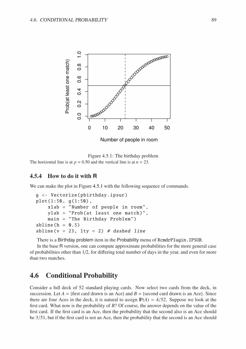
4.6. CONDITIONAL PROBABILITY 89
0 10 20 30 40 50
0.0
0.2
0.4
0.6
0.8
1.0
Number of people in room
Pro
b(a
t le
ast
one m
atc
h)
Figure 4.5.1: The birthday problemThe horizontal line is at p = 0.50 and the vertical line is at n = 23.
4.5.4 How to do it with R
We can make the plot in Figure 4.5.1 with the following sequence of commands.
g <- Vectorize(pbirthday.ipsur)
plot(1:50, g(1:50),
xlab = "Number of people in room",
ylab = "Prob(at least one match)",
main = "The Birthday Problem")
abline(h = 0.5)
abline(v = 23, lty = 2) # dashed line
There is a Birthday problem item in the Probability menu of RcmdrPlugin.IPSUR.In the base R version, one can compute approximate probabilities for the more general case
of probabilities other than 1/2, for di!ering total number of days in the year, and even for morethan two matches.
4.6 Conditional Probability
Consider a full deck of 52 standard playing cards. Now select two cards from the deck, insuccession. Let A = {first card drawn is an Ace} and B = {second card drawn is an Ace}. Sincethere are four Aces in the deck, it is natural to assign IP(A) = 4/52. Suppose we look at thefirst card. What now is the probability of B? Of course, the answer depends on the value of thefirst card. If the first card is an Ace, then the probability that the second also is an Ace shouldbe 3/51, but if the first card is not an Ace, then the probability that the second is an Ace should
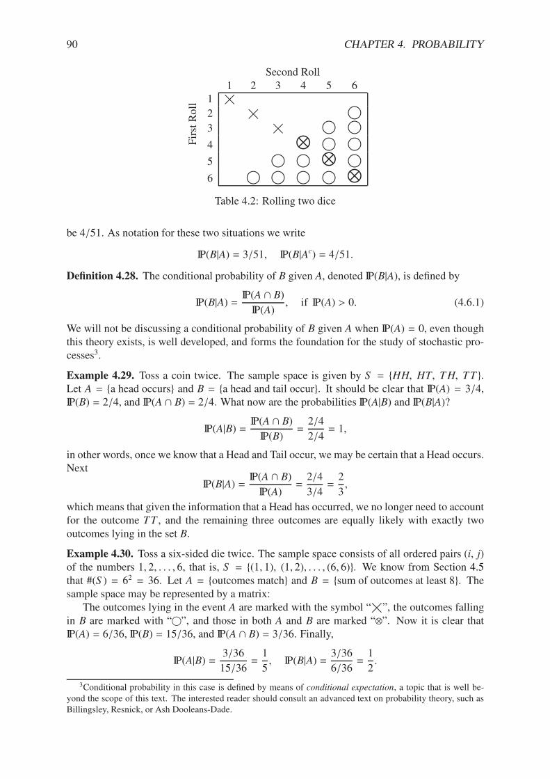
90 CHAPTER 4. PROBABILITY
FirstRoll
Second Roll1 2 3 4 5 6
1!
2! 1
3! 1 1
4 2 1 15 1 1 2 16 1 1 1 1 2Table 4.2: Rolling two dice
be 4/51. As notation for these two situations we write
IP(B|A) = 3/51, IP(B|Ac) = 4/51.
Definition 4.28. The conditional probability of B given A, denoted IP(B|A), is defined by
IP(B|A) =IP(A + B)
IP(A), if IP(A) > 0. (4.6.1)
We will not be discussing a conditional probability of B given A when IP(A) = 0, even thoughthis theory exists, is well developed, and forms the foundation for the study of stochastic pro-cesses3.
Example 4.29. Toss a coin twice. The sample space is given by S = {HH, HT, TH, TT }.Let A = {a head occurs} and B = {a head and tail occur}. It should be clear that IP(A) = 3/4,IP(B) = 2/4, and IP(A + B) = 2/4. What now are the probabilities IP(A|B) and IP(B|A)?
IP(A|B) =IP(A + B)
IP(B)=
2/4
2/4= 1,
in other words, once we know that a Head and Tail occur, we may be certain that a Head occurs.Next
IP(B|A) =IP(A + B)
IP(A)=
2/4
3/4=
2
3,
which means that given the information that a Head has occurred, we no longer need to accountfor the outcome TT , and the remaining three outcomes are equally likely with exactly twooutcomes lying in the set B.
Example 4.30. Toss a six-sided die twice. The sample space consists of all ordered pairs (i, j)of the numbers 1, 2, . . . , 6, that is, S = {(1, 1), (1, 2), . . . , (6, 6)}. We know from Section 4.5that #(S ) = 62 = 36. Let A = {outcomes match} and B = {sum of outcomes at least 8}. Thesample space may be represented by a matrix:
The outcomes lying in the event A are marked with the symbol “!
”, the outcomes fallingin B are marked with “1”, and those in both A and B are marked “2”. Now it is clear thatIP(A) = 6/36, IP(B) = 15/36, and IP(A + B) = 3/36. Finally,
IP(A|B) =3/36
15/36=
1
5, IP(B|A) =
3/36
6/36=
1
2.
3Conditional probability in this case is defined by means of conditional expectation, a topic that is well be-yond the scope of this text. The interested reader should consult an advanced text on probability theory, such asBillingsley, Resnick, or Ash Dooleans-Dade.

4.6. CONDITIONAL PROBABILITY 91
Again, we see that given the knowledge that B occurred (the 15 outcomes in the lower righttriangle), there are 3 of the 15 that fall into the set A, thus the probability is 3/15. Similarly,given that A occurred (we are on the diagonal), there are 3 out of 6 outcomes that also fall in B,thus, the probability of B given A is 1/2.
4.6.1 How to do it with R
Continuing with Example 4.30, the first thing to do is set up the probability space with therolldie function.
> library(prob)
> S <- rolldie(2, makespace = TRUE) # assumes ELM
> head(S) # first few rows
X1 X2 probs
1 1 1 0.02777778
2 2 1 0.02777778
3 3 1 0.02777778
4 4 1 0.02777778
5 5 1 0.02777778
6 6 1 0.02777778
Next we define the events
> A <- subset(S, X1 == X2)
> B <- subset(S, X1 + X2 >= 8)
And now we are ready to calculate probabilities. To do conditional probability, we use thegiven argument of the prob function:
> prob(A, given = B)
[1] 0.2
> prob(B, given = A)
[1] 0.5
Note that we do not actually need to define the events A and B separately as long as wereference the original probability space S as the first argument of the prob calculation:
> prob(S, X1==X2, given = (X1 + X2 >= 8) )
[1] 0.2
> prob(S, X1+X2 >= 8, given = (X1==X2) )
[1] 0.5
92 CHAPTER 4. PROBABILITY
4.6.2 Properties and Rules
The following theorem establishes that conditional probabilities behave just like regular prob-abilities when the conditioned event is fixed.
Theorem 4.31. For any fixed event A with IP(A) > 0,
1. IP(B|A) / 0, for all events B 0 S ,
2. IP(S |A) = 1, and
3. If B1, B2, B3,. . . are disjoint events, then
IP
$%%%%%&
&'
k=1
Bk
4444444A
()))))* =
&!
k=1
IP(Bk|A). (4.6.2)
In other words, IP(·|A) is a legitimate probability function. With this fact in mind, thefollowing properties are immediate:
Proposition 4.32. For any events A, B, and C with IP(A) > 0,
1. IP(Bc|A) = 1 # IP(B|A).
2. If B 0 C then IP(B|A) " IP(C|A).
3. IP[(B -C)|A] = IP(B|A) + IP(C|A) # IP[(B +C|A)].
4. The Multiplication Rule. For any two events A and B,
IP(A + B) = IP(A) IP(B|A). (4.6.3)
And more generally, for events A1, A2, A3,. . . , An,
IP(A1 + A2 + · · · + An) = IP(A1) IP(A2|A1) · · · IP(An|A1 + A2 + · · · + An#1). (4.6.4)
The Multiplication Rule is very important because it allows us to find probabilities in ran-dom experiments that have a sequential structure, as the next example shows.
Example 4.33. At the beginning of the section we drew two cards from a standard playingdeck. Now we may answer our original question, what is IP(both Aces)?
IP(both Aces) = IP(A + B) = IP(A) IP(B|A) =4
52·3
51' 0.00452.
4.6.3 How to do it with R
Continuing Example 4.33, we set up the probability space by way of a three step process. Firstwe employ the cards function to get a data frame L with two columns: rank and suit. Bothcolumns are stored internally as factors with 13 and 4 levels, respectively.
Next we sample two cards randomly from the L data frame by way of the urnsamples func-tion. It returns a list Mwhich contains all possible pairs of rows from L (there are choose(52,2)of them). The sample space for this experiment is exactly the list M.
4.6. CONDITIONAL PROBABILITY 93
At long last we associate a probability model with the sample space. This is right down theprobspace function’s alley. It assumes the equally likely model by default. We call this resultN which is an object of class ps – short for “probability space”.
But do not be intimidated. The object N is nothing more than a list with two elements:outcomes and probs. The outcomes element is itself just another list, with choose(52,2)entries, each one a data frame with two rows which correspond to the pair of cards chosen. Theprobs element is just a vector with choose(52,2) entries all the same: 1/choose(52,2).
Putting all of this together we do
> library(prob)
> L <- cards()
> M <- urnsamples(L, size = 2)
> N <- probspace(M)
Now that we have the probability space N we are ready to do some probability. We use theprob function, just like before. The only trick is to specify the event of interest correctly, andrecall that we were interested in IP(both Aces). But if the cards are both Aces then the rank ofboth cards should be "A", which sounds like a job for the all function:
> prob(N, all(rank == "A"))
[1] 0.004524887
Note that this value matches what we found in Example 4.33, above. We could calculateall sorts of probabilities at this point; we are limited only by the complexity of the event’scomputer representation.
Example 4.34. Consider an urn with 10 balls inside, 7 of which are red and 3 of which aregreen. Select 3 balls successively from the urn. Let A =
,1st ball is red
-, B =
52nd ball is red
6,
and C =53rd ball is red
6. Then
IP(all 3 balls are red) = IP(A + B + C) =7
10·6
9·5
8' 0.2917.
4.6.4 How to do it with R
Example 4.34 is similar to Example 4.33, but it is even easier. We need to set up an urn (vectorL) to hold the balls, we sample from L to get the sample space (data frame M), and we associatea probability vector (column probs) with the outcomes (rows of M) of the sample space. Thefinal result is a probability space (an ordinary data frame N).
It is easier for us this time because our urn is a vector instead of a cards() data frame.Before there were two dimensions of information associated with the outcomes (rank and suit)but presently we have only one dimension (color).
> library(prob)
> L <- rep(c("red", "green"), times = c(7, 3))
> M <- urnsamples(L, size = 3, replace = FALSE, ordered = TRUE)
> N <- probspace(M)
94 CHAPTER 4. PROBABILITY
Now let us think about how to set up the event {all 3 balls are red}. Rows of N that satisfythis condition have X1=="red"& X2=="red"& X3=="red", but there must be an easier way.Indeed, there is. The isrep function (short for “is repeated”) in the prob package was writtenfor this purpose. The command isrep(N,"red",3) will test each row of N to see whether thevalue "red" appears 3 times. The result is exactly what we need to define an event with theprob function. Observe
> prob(N, isrep(N, "red", 3))
[1] 0.2916667
Note that this answer matches what we found in Example 4.34. Now let us try some otherprobability questions. What is the probability of getting two "red"s?
> prob(N, isrep(N, "red", 2))
[1] 0.525
Note that the exact value is 21/40; we will learn a quick way to compute this in Section 5.6.What is the probability of observing "red", then "green", then "red"?
> prob(N, isin(N, c("red", "green", "red"), ordered = TRUE))
[1] 0.175
Note that the exact value is 7/20 (do it with theMultiplicationRule). What is the probabilityof observing "red", "green", and "red", in no particular order?
> prob(N, isin(N, c("red", "green", "red")))
[1] 0.525
We already knew this. It is the probability of observing two "red"s, above.
Example 4.35. Consider two urns, the first with 5 red balls and 3 green balls, and the sec-ond with 2 red balls and 6 green balls. Your friend randomly selects one ball from the firsturn and transfers it to the second urn, without disclosing the color of the ball. You selectone ball from the second urn. What is the probability that the selected ball is red? LetA = {transferred ball is red} and B = {selected ball is red}. Write
B = S + B
= (A - Ac) + B
= (A + B) - (Ac + B)
and notice that A + B and Ac + B are disjoint. Therefore
IP(B) = IP(A + B) + IP(Ac + B)
= IP(A) IP(B|A) + IP(Ac) IP(B|Ac)
=5
8·3
9+3
8·2
9
=21
72
(which is 7/24 in lowest terms).
4.7. INDEPENDENT EVENTS 95
Example 4.36. We saw the RcmdrTestDrive data set in Chapter 2 in which a two-way tableof the smoking status versus the gender was
gender
smoke Female Male Sum
No 80 54 134
Yes 15 19 34
Sum 95 73 168
If one person were selected at random from the data set, then we see from the two-way tablethat IP(Female) = 70/168 and IP(Smoker) = 32/168. Now suppose that one of the subjectsquits smoking, but we do not know the person’s gender. If we select one subject at random, whatnow is IP(Female)? Let A =
,the quitter is a female
-and B =
,selected person is a female
-.
Write
B = S + B
= (A - Ac) + B
= (A + B) - (Ac + B)
and notice that A + B and Ac + B are disjoint. Therefore
IP(B) = IP(A + B) + IP(Ac + B),
= IP(A) IP(B|A) + IP(Ac) IP(B|Ac),
=5
8·3
9+3
8·2
9,
=21
72,
(which is 7/24 in lowest terms).
Using the same reasoning, we can return to the example from the beginning of the sectionand show that
IP({second card is an Ace}) = 4/52.
.
4.7 Independent Events
Toss a coin twice. The sample space is S = {HH, HT, TH, TT }. We know that IP(1st toss is H) =2/4, IP(2nd toss is H) = 2/4, and IP(both H) = 1/4. Then
IP(2nd toss is H | 1st toss is H) =IP(both H)
IP(1st toss is H),
=1/4
2/4,
= IP(2nd toss is H).
Intuitively, this means that the information that the first toss is H has no bearing on the proba-bility that the second toss is H. The coin does not remember the result of the first toss.
96 CHAPTER 4. PROBABILITY
Definition 4.37. Events A and B are said to be independent if
IP(A + B) = IP(A) IP(B). (4.7.1)
Otherwise, the events are said to be dependent.
The connection with the above example stems from the following. We know from Section4.6 that when IP(B) > 0 we may write
IP(A|B) =IP(A + B)
IP(B). (4.7.2)
In the case that A and B are independent, the numerator of the fraction factors so that IP(B)cancels with the result:
IP(A|B) = IP(A) when A, B are independent. (4.7.3)
The interpretation in the case of independence is that the information that the event B occurreddoes not influence the probability of the event A occurring. Similarly, IP(B|A) = IP(B), andso the occurrence of the event A likewise does not a!ect the probability of event B. It mayseem more natural to define A and B to be independent when IP(A|B) = IP(A); however, theconditional probability IP(A|B) is only defined when IP(B) > 0. Our definition is not limited bythis restriction. It can be shown that when IP(A), IP(B) > 0 the two notions of independenceare equivalent.
Proposition 4.38. If the events A and B are independent then
• A and Bc are independent,
• Ac and B are independent,
• Ac and Bc are independent.
Proof. Suppose that A and B are independent. We will show the second one; the others aresimilar. We need to show that
IP(Ac + B) = IP(Ac) IP(B).
To this end, note that the Multiplication Rule, Equation 4.6.3 implies
IP(Ac + B) = IP(B) IP(Ac|B),= IP(B)[1 # IP(A|B)],= IP(B) IP(Ac).
"
Definition 4.39. The events A, B, and C are mutually independent if the following four condi-tions are met:
IP(A + B) = IP(A) IP(B),
IP(A + C) = IP(A) IP(C),
IP(B + C) = IP(B) IP(C),
andIP(A + B +C) = IP(A) IP(B) IP(C).
If only the first three conditions hold then A, B, and C are said to be independent pairwise.Note that pairwise independence is not the same as mutual independence when the number ofevents is larger than two.
4.7. INDEPENDENT EVENTS 97
We can now deduce the pattern for n events, n > 3. The events will be mutually independentonly if they satisfy the product equality pairwise, then in groups of three, in groups of four, andso forth, up to all n events at once. For n events, there will be 2n # n # 1 equations that mustbe satisfied (see Exercise 4.1). Although these requirements for a set of events to be mutuallyindependent may seem stringent, the good news is that for most of the situations considered inthis book the conditions will all be met (or at least we will suppose that they are).
Example 4.40. Toss ten coins. What is the probability of observing at least one Head? Answer:Let Ai =
5the ith coin shows H
6, i = 1, 2, . . . , 10. Supposing that we toss the coins in such a
way that they do not interfere with each other, this is one of the situations where all of the Ai
may be considered mutually independent due to the nature of the tossing. Of course, the onlyway that there will not be at least one Head showing is if all tosses are Tails. Therefore,
IP(at least one H) = 1 # IP(all T ),
= 1 # IP(Ac1 + Ac
2 + · · · + Ac10),
= 1 # IP(Ac1) IP(A
c2) · · · IP(A
c10),
= 1 #01
2
110,
which is approximately 0.9990234.
4.7.1 How to do it with R
Example 4.41. Toss ten coins. What is the probability of observing at least one Head?
> S <- tosscoin(10, makespace = TRUE)
> A <- subset(S, isrep(S, vals = "T", nrep = 10))
> 1 - prob(A)
[1] 0.9990234
Compare this answer to what we got in Example 4.40.
Independent, Repeated Experiments
Generalizing from above it is common to repeat a certain experiment multiple times under iden-tical conditions and in an independent manner. We have seen many examples of this already:tossing a coin repeatedly, rolling a die or dice, etc.
The iidspace function was designed specifically for this situation. It has three arguments:x, which is a vector of outcomes, ntrials, which is an integer telling how many times torepeat the experiment, and probs to specify the probabilities of the outcomes of x in a singletrial.
Example 4.42. An unbalanced coin (continued, see Example 4.5). It was easy enough toset up the probability space for one unbalanced toss, however, the situation becomes morecomplicated when there are many tosses involved. Clearly, the outcome HHH should not havethe same probability as TTT , which should again not have the same probability as HTH. Atthe same time, there is symmetry in the experiment in that the coin does not remember the faceit shows from toss to toss, and it is easy enough to toss the coin in a similar way repeatedly.
We may represent tossing our unbalanced coin three times with the following:
98 CHAPTER 4. PROBABILITY
> iidspace(c("H","T"), ntrials = 3, probs = c(0.7, 0.3))
X1 X2 X3 probs
1 H H H 0.343
2 T H H 0.147
3 H T H 0.147
4 T T H 0.063
5 H H T 0.147
6 T H T 0.063
7 H T T 0.063
8 T T T 0.027
As expected, the outcome HHH has the largest probability, while TTT has the smallest.(Since the trials are independent, IP(HHH) = 0.73 and IP(TTT ) = 0.33, etc.) Note that theresult of the function call is a probability space, not a sample space (which we could constructalready with the tosscoin or urnsamples functions). The same procedure could be used tomodel an unbalanced die or any other experiment that may be represented with a vector ofpossible outcomes.
Note that iidspace will assume x has equally likely outcomes if no probs argumentis specified. Also note that the argument x is a vector, not a data frame. Something likeiidspace(tosscoin(1),...) would give an error.
4.8 Bayes’ Rule
We mentioned the subjective view of probability in Section 4.3. In this section we introduce arule that allows us to update our probabilities when new information becomes available.
Theorem 4.43. (Bayes’ Rule). Let B1, B2, . . . , Bn be mutually exclusive and exhaustive and
let A be an event with IP(A) > 0. Then
IP(Bk|A) =IP(Bk) IP(A|Bk)#ni=1 IP(Bi) IP(A|Bi)
, k = 1, 2, . . . , n. (4.8.1)
Proof. The proof follows from looking at IP(Bk + A) in two di!erent ways. For simplicity,suppose that P(Bk) > 0 for all k. Then
IP(A) IP(Bk|A) = IP(Bk + A) = IP(Bk) IP(A|Bk).
Since IP(A) > 0 we may divide through to obtain
IP(Bk|A) =IP(Bk) IP(A|Bk)
IP(A).
Now remembering that {Bk} is a partition, the Theorem of Total Probability (Equation 4.4.5)gives the denominator of the last expression to be
IP(A) =n!
k=1
IP(Bk + A) =n!
k=1
IP(Bk) IP(A|Bk).
"
4.8. BAYES’ RULE 99
What does it mean? Usually in applications we are given (or know) a priori probabilitiesIP(Bk). We go out and collect some data, which we represent by the event A. We want to know:how do we update IP(Bk) to IP(Bk|A)? The answer: Bayes’ Rule.
Example 4.44. Misfiling Assistants. In this problem, there are three assistants working at acompany: Moe, Larry, and Curly. Their primary job duty is to file paperwork in the filingcabinet when papers become available. The three assistants have di!erent work schedules:
Moe Larry CurlyWorkload 60% 30% 10%
That is, Moe works 60% of the time, Larry works 30% of the time, and Curly does theremaining 10%, and they file documents at approximately the same speed. Suppose a personwere to select one of the documents from the cabinet at random. Let M be the event
M = {Moe filed the document}
and let L and C be the events that Larry and Curly, respectively, filed the document. Whatare these events’ respective probabilities? In the absence of additional information, reasonableprior probabilities would just be
Moe Larry CurlyPrior Probability IP(M) = 0.60 IP(L) = 0.30 IP(C) = 0.10
Now, the boss comes in one day, opens up the file cabinet, and selects a file at random. Theboss discovers that the file has been misplaced. The boss is so angry at the mistake that (s)hethreatens to fire the one who erred. The question is: who misplaced the file?
The boss decides to use probability to decide, and walks straight to the workload schedule.(S)he reasons that, since the three employees work at the same speed, the probability that a ran-domly selected file would have been filed by each one would be proportional to his workload.The boss notifiesMoe that he has until the end of the day to empty his desk.
But Moe argues in his defense that the boss has ignored additional information. Moe’slikelihood of having misfiled a document is smaller than Larry’s and Curly’s, since he is adiligent worker who pays close attention to his work. Moe admits that he works longer thanthe others, but he doesn’t make as many mistakes as they do. Thus, Moe recommends that –before making a decision – the boss should update the probability (initially based on workloadalone) to incorporate the likelihood of having observed a misfiled document.
And, as it turns out, the boss has information about Moe, Larry, and Curly’s filing accuracyin the past (due to historical performance evaluations). The performance information may berepresented by the following table:
Moe Larry CurlyMisfile Rate 0.003 0.007 0.010
In other words, on the average, Moe misfiles 0.3% of the documents he is supposed to file.Notice that Moe was correct: he is the most accurate filer, followed by Larry, and lastly Curly.If the boss were to make a decision based only on the worker’s overall accuracy, then Curly
should get the axe. But Curly hears this and interjects that he only works a short period during
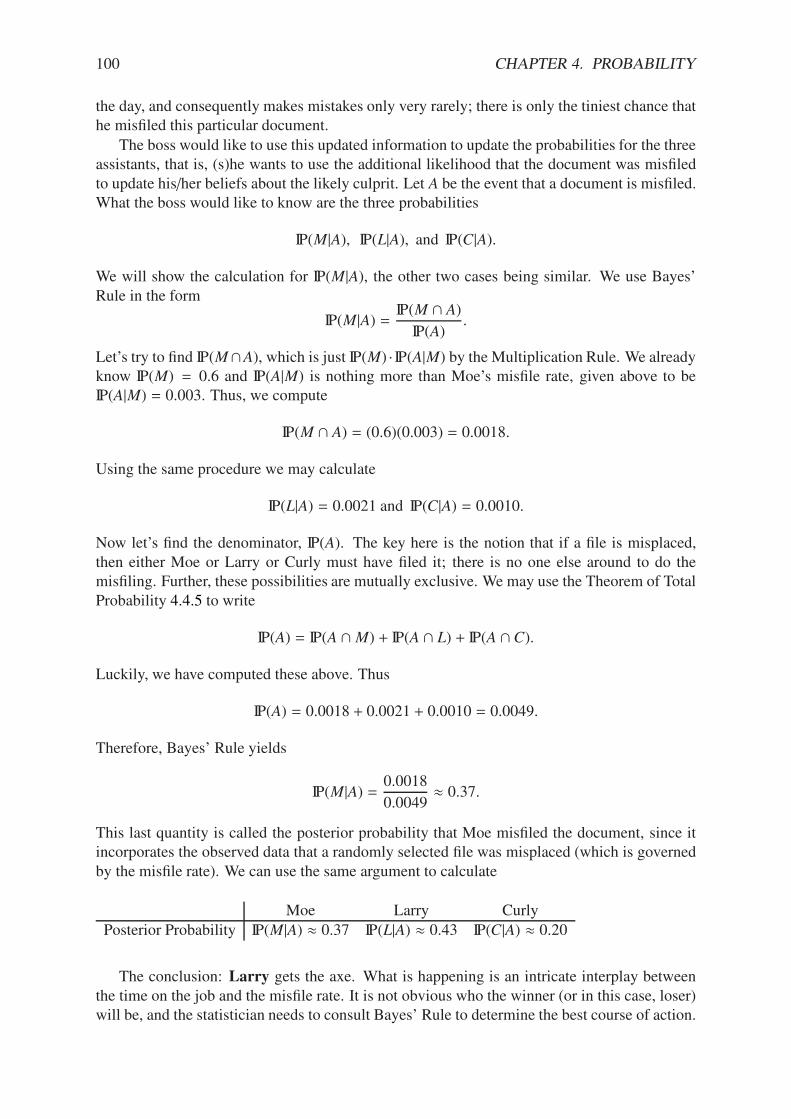
100 CHAPTER 4. PROBABILITY
the day, and consequently makes mistakes only very rarely; there is only the tiniest chance thathe misfiled this particular document.
The boss would like to use this updated information to update the probabilities for the threeassistants, that is, (s)he wants to use the additional likelihood that the document was misfiledto update his/her beliefs about the likely culprit. Let A be the event that a document is misfiled.What the boss would like to know are the three probabilities
IP(M|A), IP(L|A), and IP(C|A).
We will show the calculation for IP(M|A), the other two cases being similar. We use Bayes’Rule in the form
IP(M|A) =IP(M + A)
IP(A).
Let’s try to find IP(M+A), which is just IP(M) · IP(A|M) by the Multiplication Rule. We alreadyknow IP(M) = 0.6 and IP(A|M) is nothing more than Moe’s misfile rate, given above to beIP(A|M) = 0.003. Thus, we compute
IP(M + A) = (0.6)(0.003) = 0.0018.
Using the same procedure we may calculate
IP(L|A) = 0.0021 and IP(C|A) = 0.0010.
Now let’s find the denominator, IP(A). The key here is the notion that if a file is misplaced,then either Moe or Larry or Curly must have filed it; there is no one else around to do themisfiling. Further, these possibilities are mutually exclusive. We may use the Theorem of TotalProbability 4.4.5 to write
IP(A) = IP(A + M) + IP(A + L) + IP(A +C).
Luckily, we have computed these above. Thus
IP(A) = 0.0018 + 0.0021 + 0.0010 = 0.0049.
Therefore, Bayes’ Rule yields
IP(M|A) =0.0018
0.0049' 0.37.
This last quantity is called the posterior probability that Moe misfiled the document, since itincorporates the observed data that a randomly selected file was misplaced (which is governedby the misfile rate). We can use the same argument to calculate
Moe Larry CurlyPosterior Probability IP(M|A) ' 0.37 IP(L|A) ' 0.43 IP(C|A) ' 0.20
The conclusion: Larry gets the axe. What is happening is an intricate interplay betweenthe time on the job and the misfile rate. It is not obvious who the winner (or in this case, loser)will be, and the statistician needs to consult Bayes’ Rule to determine the best course of action.
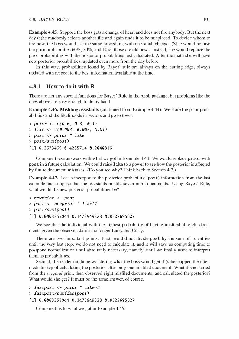
4.8. BAYES’ RULE 101
Example 4.45. Suppose the boss gets a change of heart and does not fire anybody. But the nextday (s)he randomly selects another file and again finds it to be misplaced. To decide whom tofire now, the boss would use the same procedure, with one small change. (S)he would not usethe prior probabilities 60%, 30%, and 10%; those are old news. Instead, she would replace theprior probabilities with the posterior probabilities just calculated. After the math she will havenew posterior probabilities, updated even more from the day before.
In this way, probabilities found by Bayes’ rule are always on the cutting edge, alwaysupdated with respect to the best information available at the time.
4.8.1 How to do it with R
There are not any special functions for Bayes’ Rule in the prob package, but problems like theones above are easy enough to do by hand.
Example 4.46. Misfiling assistants (continued from Example 4.44). We store the prior prob-abilities and the likelihoods in vectors and go to town.
> prior <- c(0.6, 0.3, 0.1)
> like <- c(0.003, 0.007, 0.01)
> post <- prior * like
> post/sum(post)
[1] 0.3673469 0.4285714 0.2040816
Compare these answers with what we got in Example 4.44. We would replace prior withpost in a future calculation. We could raise like to a power to see how the posterior is a!ectedby future document mistakes. (Do you see why? Think back to Section 4.7.)
Example 4.47. Let us incorporate the posterior probability (post) information from the lastexample and suppose that the assistants misfile seven more documents. Using Bayes’ Rule,what would the new posterior probabilities be?
> newprior <- post
> post <- newprior * like^7
> post/sum(post)
[1] 0.0003355044 0.1473949328 0.8522695627
We see that the individual with the highest probability of having misfiled all eight docu-ments given the observed data is no longer Larry, but Curly.
There are two important points. First, we did not divide post by the sum of its entriesuntil the very last step; we do not need to calculate it, and it will save us computing time topostpone normalization until absolutely necessary, namely, until we finally want to interpretthem as probabilities.
Second, the reader might be wondering what the boss would get if (s)he skipped the inter-mediate step of calculating the posterior after only one misfiled document. What if she startedfrom the original prior, then observed eight misfiled documents, and calculated the posterior?What would she get? It must be the same answer, of course.
> fastpost <- prior * like^8
> fastpost/sum(fastpost)
[1] 0.0003355044 0.1473949328 0.8522695627
Compare this to what we got in Example 4.45.
102 CHAPTER 4. PROBABILITY
4.9 Random Variables
We already know about experiments, sample spaces, and events. In this section, we are inter-ested in a number that is associated with the experiment. We conduct a random experiment Eand after learning the outcome # in S we calculate a number X. That is, to each outcome # inthe sample space we associate a number X(#) = x.
Definition 4.48. A random variable X is a function X : S . R that associates to each outcome# 3 S exactly one number X(#) = x.
We usually denote random variables by uppercase letters such as X, Y , and Z, and wedenote their observed values by lowercase letters x, y, and z. Just as S is the set of all possibleoutcomes of E, we call the set of all possible values of X the support of X and denote it by S X.
Example 4.49. Let E be the experiment of flipping a coin twice. We have seen that the samplespace is S = {HH, HT, TH, TT }. Now define the random variable X = the number of heads.That is, for example, X(HH) = 2, while X(HT ) = 1. We may make a table of the possibilities:
# 3 S HH HT TH TT
X(#) = x 2 1 1 0
Taking a look at the second row of the table, we see that the support of X – the set of allnumbers that X assumes – would be S X = {0, 1, 2}.
Example 4.50. Let E be the experiment of flipping a coin repeatedly until observing a Head.The sample space would be S = {H, TH, TTH, TTTH, . . .}. Now define the random vari-able Y = the number of Tails before the first head. Then the support of Y would be S Y =
{0, 1, 2, . . .}.
Example 4.51. Let E be the experiment of tossing a coin in the air, and define the randomvariable Z = the time (in seconds) until the coin hits the ground. In this case, the sample spaceis inconvenient to describe. Yet the support of Z would be (0,&). Of course, it is reasonable tosuppose that the coin will return to Earth in a short amount of time; in practice, the set (0,&)is admittedly too large. However, we will find that in many circumstances it is mathematicallyconvenient to study the extended set rather than a restricted one.
There are important di!erences between the supports of X, Y , and Z. The support of Xis a finite collection of elements that can be inspected all at once. And while the support ofY cannot be exhaustively written down, its elements can nevertheless be listed in a naturallyordered sequence. Random variables with supports similar to those of X and Y are calleddiscrete random variables. We study these in Chapter 5.
In contrast, the support of Z is a continuous interval, containing all rational and irrationalpositive real numbers. For this reason4, random variables with supports like Z are called con-
tinuous random variables, to be studied in Chapter 6.
4.9.1 How to do it with R
The primary vessel for this task is the addrv function. There are two ways to use it, and wewill describe both.
4This isn’t really the reason, but it serves as an e!ective litmus test at the introductory level. See Billingsley orResnick.

4.9. RANDOM VARIABLES 103
Supply a Defining Formula
The first method is based on the transform function. See ?transform. The idea is to writea formula defining the random variable inside the function, and it will be added as a column tothe data frame. As an example, let us roll a 4-sided die three times, and let us define the randomvariable U = X1 # X2 + X3.
> S <- rolldie(3, nsides = 4, makespace = TRUE)
> S <- addrv(S, U = X1 - X2 + X3)
Now let’s take a look at the values of U. In the interest of space, we will only reproduce thefirst few rows of S (there are 43 = 64 rows in total).
> head(S)
X1 X2 X3 U probs
1 1 1 1 1 0.015625
2 2 1 1 2 0.015625
3 3 1 1 3 0.015625
4 4 1 1 4 0.015625
5 1 2 1 0 0.015625
6 2 2 1 1 0.015625
We see from the U column it is operating just like it should. We can now answer questionslike
> prob(S, U > 6)
[1] 0.015625
Supply a Function
Sometimes we have a function laying around that we would like to apply to some of the out-come variables, but it is unfortunately tedious to write out the formula defining what the newvariable would be. The addrv function has an argument FUN specifically for this case. Its valueshould be a legitimate function from R, such as sum, mean, median, etc. Or, you can defineyour own function. Continuing the previous example, let’s define V = max(X1, X2, X3) andW = X1 + X2 + X3.
> S <- addrv(S, FUN = max, invars = c("X1", "X2", "X3"), name = "V")
> S <- addrv(S, FUN = sum, invars = c("X1", "X2", "X3"), name = "W")
> head(S)
X1 X2 X3 U V W probs
1 1 1 1 1 1 3 0.015625
2 2 1 1 2 2 4 0.015625
3 3 1 1 3 3 5 0.015625
4 4 1 1 4 4 6 0.015625
5 1 2 1 0 2 4 0.015625
6 2 2 1 1 2 5 0.015625
Notice that addrv has an invars argument to specify exactly to which columns one wouldlike to apply the function FUN. If no input variables are specified, then addrv will apply FUNto all non-probs columns. Further, addrv has an optional argument name to give the newvariable; this can be useful when adding several random variables to a probability space (asabove). If not specified, the default name is “X”.
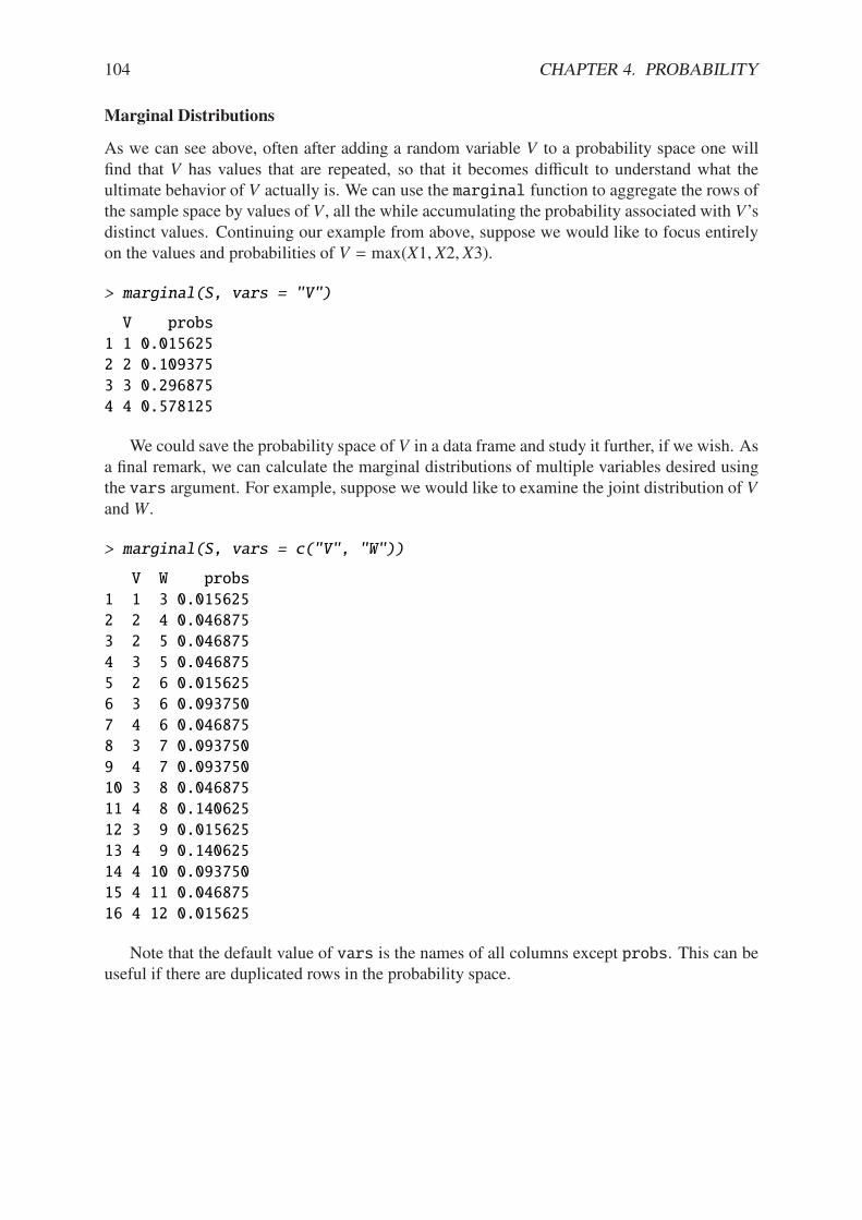
104 CHAPTER 4. PROBABILITY
Marginal Distributions
As we can see above, often after adding a random variable V to a probability space one willfind that V has values that are repeated, so that it becomes di"cult to understand what theultimate behavior of V actually is. We can use the marginal function to aggregate the rows ofthe sample space by values of V , all the while accumulating the probability associated with V’sdistinct values. Continuing our example from above, suppose we would like to focus entirelyon the values and probabilities of V = max(X1, X2, X3).
> marginal(S, vars = "V")
V probs
1 1 0.015625
2 2 0.109375
3 3 0.296875
4 4 0.578125
We could save the probability space of V in a data frame and study it further, if we wish. Asa final remark, we can calculate the marginal distributions of multiple variables desired usingthe vars argument. For example, suppose we would like to examine the joint distribution of Vand W.
> marginal(S, vars = c("V", "W"))
V W probs
1 1 3 0.015625
2 2 4 0.046875
3 2 5 0.046875
4 3 5 0.046875
5 2 6 0.015625
6 3 6 0.093750
7 4 6 0.046875
8 3 7 0.093750
9 4 7 0.093750
10 3 8 0.046875
11 4 8 0.140625
12 3 9 0.015625
13 4 9 0.140625
14 4 10 0.093750
15 4 11 0.046875
16 4 12 0.015625
Note that the default value of vars is the names of all columns except probs. This can beuseful if there are duplicated rows in the probability space.

4.9. RANDOM VARIABLES 105
Chapter Exercises
Exercise 4.1. Prove the assertion given in the text: the number of conditions that the events A1,A2, . . . , An must satisfy in order to be mutually independent is 2n # n # 1. (Hint: think aboutPascal’s triangle.)
Answer: The events must satisfy the product equalities two at a time, of which there are2n2
3,
then they must satisfy an additional2n3
3conditions three at a time, and so on, until they satisfy
the2nn
3= 1 condition including all n events. In total, there are
0n
2
1+
0n
3
1+ · · · +
0n
n
1=
n!
k=0
0n
k
1#
70n
0
1+
0n
1
18
conditions to be satisfied, but the binomial series in the expression on the right is the sum ofthe entries of the nth row of Pascal’s triangle, which is 2n.

106 CHAPTER 4. PROBABILITY
Chapter 5
Discrete Distributions
In this chapter we introduce discrete random variables, those who take values in a finite orcountably infinite support set. We discuss probability mass functions and some special ex-pectations, namely, the mean, variance and standard deviation. Some of the more importantdiscrete distributions are explored in detail, and the more general concept of expectation isdefined, which paves the way for moment generating functions.
We give special attention to the empirical distribution since it plays such a fundamentalrole with respect to re sampling and Chapter 13; it will also be needed in Section 10.5.1 wherewe discuss the Kolmogorov-Smirnov test. Following this is a section in which we introduce acatalogue of discrete random variables that can be used to model experiments.
There are some comments on simulation, and we mention transformations of random vari-ables in the discrete case. The interested reader who would like to learn more about any ofthe assorted discrete distributions mentioned here should take a look at Univariate Discrete
Distributions by Johnson et al [50].
What do I want them to know?
• how to choose a reasonable discrete model under a variety of physical circumstances
• the notion of mathematical expectation, how to calculate it, and basic properties
• moment generating functions (yes, I want them to hear about those)
• the general tools of the trade for manipulation of continuous random variables, integra-tion, etc.
• some details on a couple of discrete models, and exposure to a bunch of other ones
• how to make new discrete random variables from old ones
5.1 Discrete Random Variables
5.1.1 Probability Mass Functions
Discrete random variables are characterized by their supports which take the form
S X = {u1, u2, . . . , uk} or S X = {u1, u2, u3 . . .}. (5.1.1)
107

108 CHAPTER 5. DISCRETE DISTRIBUTIONS
Every discrete random variable X has associated with it a probability mass function (PMF)fX : S X . [0, 1] defined by
fX(x) = IP(X = x), x 3 S X. (5.1.2)
Since values of the PMF represent probabilities, we know from Chapter 4 that PMFs enjoycertain properties. In particular, all PMFs satisfy
1. fX(x) > 0 for x 3 S ,
2.#
x3S fX(x) = 1, and
3. IP(X 3 A) =#
x3A fX(x), for any event A 0 S .
Example 5.1. Toss a coin 3 times. The sample space would be
S = {HHH, HTH, THH, TTH, HHT, HTT, THT, TTT } .
Now let X be the number of Heads observed. Then X has support S X = {0, 1, 2, 3}. Assumingthat the coin is fair and was tossed in exactly the same way each time, it is not unreasonableto suppose that the outcomes in the sample space are all equally likely. What is the PMF ofX? Notice that X is zero exactly when the outcome TTT occurs, and this event has probability1/8. Therefore, fX(0) = 1/8, and the same reasoning shows that fX(3) = 1/8. Exactly threeoutcomes result in X = 1, thus, fX(1) = 3/8 and fX(3) holds the remaining 3/8 probability (thetotal is 1). We can represent the PMF with a table:
x 3 S X 0 1 2 3 TotalfX(x) = IP(X = x) 1/8 3/8 3/8 1/8 1
5.1.2 Mean, Variance, and Standard Deviation
There are numbers associated with PMFs. One important example is the mean µ, also knownas IE X:
µ = IE X =!
x3S
x fX(x), (5.1.3)
provided the (potentially infinite) series#|x| fX(x) is convergent. Another important number is
the variance:"2 = IE(X # µ)2 =
!
x3S
(x # µ)2 fX(x), (5.1.4)
which can be computed (see Exercise 5.4) with the alternate formula "2 = IE X2 # (IE X)2.Directly defined from the variance is the standard deviation " =
$"2.
Example 5.2. We will calculate the mean of X in Example 5.1.
µ =
3!
x=0
x fX(x) = 0 ·1
8+ 1 ·
3
8+ 2 ·
3
8+ 3 ·
1
8= 3.5.
We interpret µ = 3.5 by reasoning that if we were to repeat the random experiment many times,independently each time, observe many corresponding outcomes of the random variable X, andtake the sample mean of the observations, then the calculated value would fall close to 3.5. Theapproximation would get better as we observe more and more values of X (another form of theLaw of Large Numbers; see Section 4.3). Another way it is commonly stated is that X is 3.5“on the average” or “in the long run”.
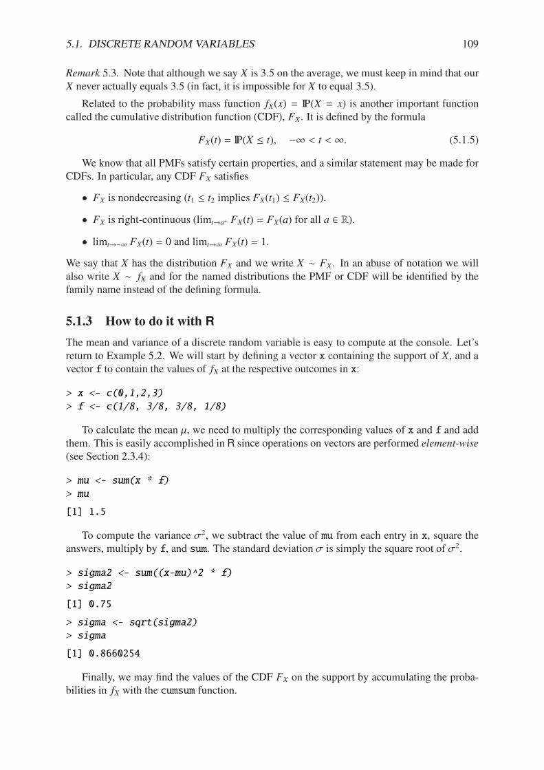
5.1. DISCRETE RANDOM VARIABLES 109
Remark 5.3. Note that although we say X is 3.5 on the average, we must keep in mind that ourX never actually equals 3.5 (in fact, it is impossible for X to equal 3.5).
Related to the probability mass function fX(x) = IP(X = x) is another important functioncalled the cumulative distribution function (CDF), FX. It is defined by the formula
FX(t) = IP(X " t), #& < t < &. (5.1.5)
We know that all PMFs satisfy certain properties, and a similar statement may be made forCDFs. In particular, any CDF FX satisfies
• FX is nondecreasing (t1 " t2 implies FX(t1) " FX(t2)).
• FX is right-continuous (limt.a+ FX(t) = FX(a) for all a 3 R).
• limt.#& FX(t) = 0 and limt.& FX(t) = 1.
We say that X has the distribution FX and we write X 4 FX. In an abuse of notation we willalso write X 4 fX and for the named distributions the PMF or CDF will be identified by thefamily name instead of the defining formula.
5.1.3 How to do it with R
The mean and variance of a discrete random variable is easy to compute at the console. Let’sreturn to Example 5.2. We will start by defining a vector x containing the support of X, and avector f to contain the values of fX at the respective outcomes in x:
> x <- c(0,1,2,3)
> f <- c(1/8, 3/8, 3/8, 1/8)
To calculate the mean µ, we need to multiply the corresponding values of x and f and addthem. This is easily accomplished in R since operations on vectors are performed element-wise(see Section 2.3.4):
> mu <- sum(x * f)
> mu
[1] 1.5
To compute the variance "2, we subtract the value of mu from each entry in x, square theanswers, multiply by f, and sum. The standard deviation " is simply the square root of "2.
> sigma2 <- sum((x-mu)^2 * f)
> sigma2
[1] 0.75
> sigma <- sqrt(sigma2)
> sigma
[1] 0.8660254
Finally, we may find the values of the CDF FX on the support by accumulating the proba-bilities in fX with the cumsum function.
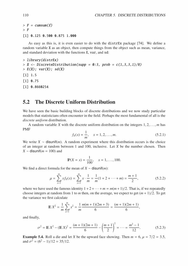
110 CHAPTER 5. DISCRETE DISTRIBUTIONS
> F = cumsum(f)
> F
[1] 0.125 0.500 0.875 1.000
As easy as this is, it is even easier to do with the distrEx package [74]. We define arandom variable X as an object, then compute things from the object such as mean, variance,and standard deviation with the functions E, var, and sd:
> library(distrEx)
> X <- DiscreteDistribution(supp = 0:3, prob = c(1,3,3,1)/8)
> E(X); var(X); sd(X)
[1] 1.5
[1] 0.75
[1] 0.8660254
5.2 The Discrete Uniform Distribution
We have seen the basic building blocks of discrete distributions and we now study particularmodels that statisticians often encounter in the field. Perhaps the most fundamental of all is thediscrete uniform distribution.
A random variable X with the discrete uniform distribution on the integers 1, 2, . . . ,m hasPMF
fX(x) =1
m, x = 1, 2, . . . ,m. (5.2.1)
We write X 4 disunif(m). A random experiment where this distribution occurs is the choiceof an integer at random between 1 and 100, inclusive. Let X be the number chosen. ThenX 4 disunif(m = 100) and
IP(X = x) =1
100, x = 1, . . . , 100.
We find a direct formula for the mean of X 4 disunif(m):
µ =
m!
x=1
x fX(x) =m!
x=1
x ·1
m=
1
m(1 + 2 + · · · + m) =
m + 1
2, (5.2.2)
where we have used the famous identity 1+ 2+ · · ·+m = m(m+ 1)/2. That is, if we repeatedlychoose integers at random from 1 to m then, on the average, we expect to get (m + 1)/2. To getthe variance we first calculate
IE X2 =1
m
m!
x=1
x2 =1
m
m(m + 1)(2m + 3)
6=
(m + 1)(2m + 1)
6,
and finally,
"2 = IE X2 # (IE X)2 =(m + 1)(2m + 1)
6#
0m + 1
2
12= · · · =
m2 # 1
12. (5.2.3)
Example 5.4. Roll a die and let X be the upward face showing. Then m = 6, µ = 7/2 = 3.5,and "2 = (62 # 1)/12 = 35/12.

5.3. THE BINOMIAL DISTRIBUTION 111
5.2.1 How to do it with R
From the console: One can choose an integer at random with the sample function. The gen-eral syntax to simulate a discrete uniform random variable is sample(x, size, replace= TRUE).
The argument x identifies the numbers from which to randomly sample. If x is a number,then sampling is done from 1 to x. The argument size tells how big the sample size shouldbe, and replace tells whether or not numbers should be replaced in the urn after having beensampled. The default option is replace = FALSE but for discrete uniforms the sampled valuesshould be replaced. Some examples follow.
5.2.2 Examples
• To roll a fair die 3000 times, do sample(6, size = 3000, replace = TRUE).
• To choose 27 random numbers from 30 to 70, do sample(30:70, size = 27, replace= TRUE).
• To flip a fair coin 1000 times, do sample(c("H","T"), size = 1000, replace =TRUE).
With the R Commander: Follow the sequence Probability ! Discrete Distributions ! Dis-crete Uniform distribution ! Simulate Discrete uniform variates. . . .
Suppose we would like to roll a fair die 3000 times. In the Number of samples field weenter 1. Next, we describe what interval of integers to be sampled. Since there are six facesnumbered 1 through 6, we set from = 1, we set to = 6, and set by = 1 (to indicate that wetravel from 1 to 6 in increments of 1 unit). We will generate a list of 3000 numbers selectedfrom among 1, 2, . . . , 6, and we store the results of the simulation. For the time being, weselect New Data set. Click OK.
Since we are defining a new data set, theRCommander requests a name for the data set. Thedefault name is Simset1, although in principle you could name it whatever you like (accordingto R’s rules for object names). We wish to have a list that is 3000 long, so we set SampleSize = 3000 and click OK.
In the R Console window, the R Commander should tell you that Simset1 has been initial-ized, and it should also alert you that There was 1 discrete uniform variate samplestored in Simset 1.. To take a look at the rolls of the die, we click View data set and awindow opens.
The default name for the variable is disunif.sim1.
5.3 The Binomial Distribution
The binomial distribution is based on a Bernoulli trial, which is a random experiment in whichthere are only two possible outcomes: success (S ) and failure (F). We conduct the Bernoullitrial and let
X =
9::;::<1 if the outcome is S ,
0 if the outcome is F.(5.3.1)
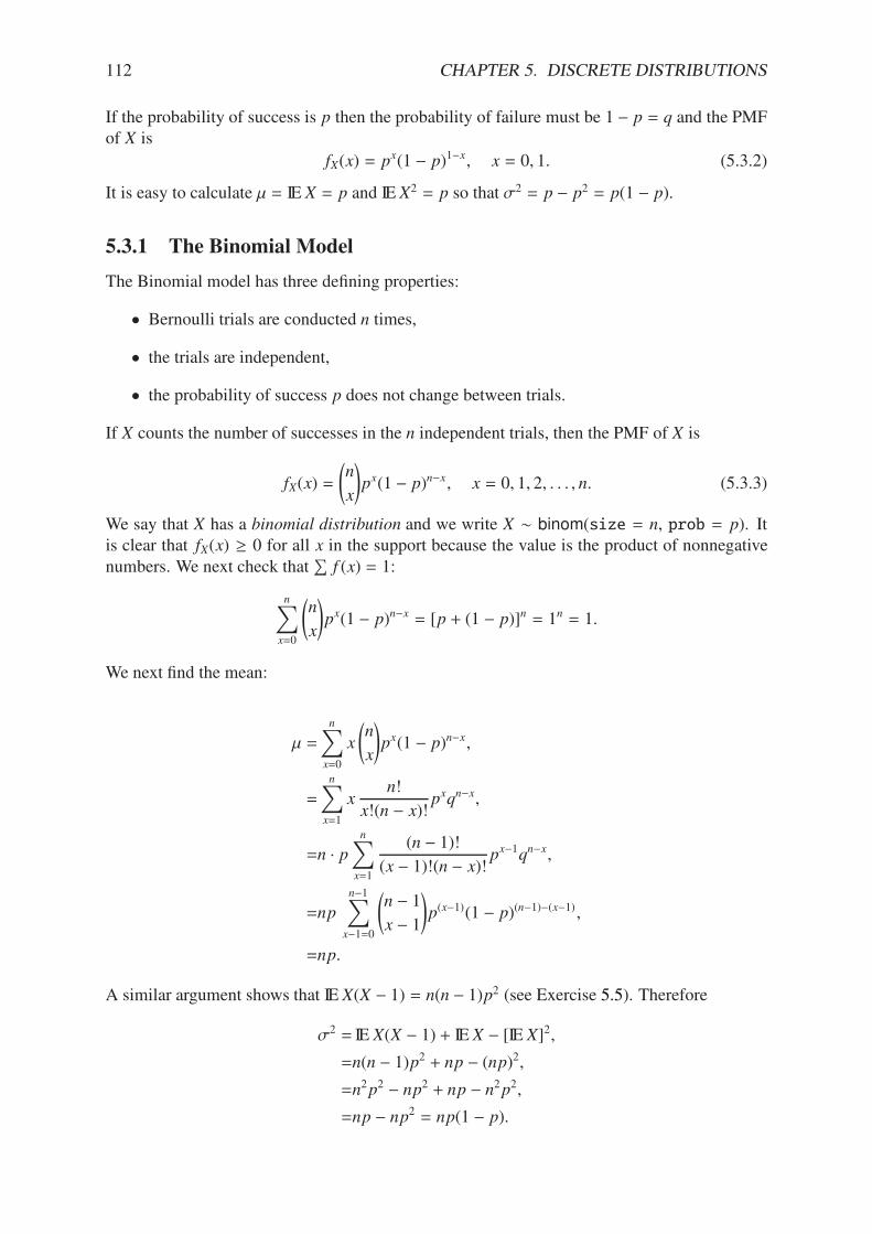
112 CHAPTER 5. DISCRETE DISTRIBUTIONS
If the probability of success is p then the probability of failure must be 1 # p = q and the PMFof X is
fX(x) = px(1 # p)1#x, x = 0, 1. (5.3.2)
It is easy to calculate µ = IE X = p and IE X2 = p so that "2 = p # p2 = p(1 # p).
5.3.1 The Binomial Model
The Binomial model has three defining properties:
• Bernoulli trials are conducted n times,
• the trials are independent,
• the probability of success p does not change between trials.
If X counts the number of successes in the n independent trials, then the PMF of X is
fX(x) =
0n
x
1px(1 # p)n#x, x = 0, 1, 2, . . . , n. (5.3.3)
We say that X has a binomial distribution and we write X 4 binom(size = n, prob = p). Itis clear that fX(x) / 0 for all x in the support because the value is the product of nonnegativenumbers. We next check that
#f (x) = 1:
n!
x=0
0n
x
1px(1 # p)n#x = [p + (1 # p)]n = 1n = 1.
We next find the mean:
µ =
n!
x=0
x
0n
x
1px(1 # p)n#x,
=
n!
x=1
xn!
x!(n # x)!pxqn#x,
=n · pn!
x=1
(n # 1)!
(x # 1)!(n # x)!px#1qn#x,
=np
n#1!
x#1=0
0n # 1
x # 1
1p(x#1)(1 # p)(n#1)#(x#1) ,
=np.
A similar argument shows that IE X(X # 1) = n(n # 1)p2 (see Exercise 5.5). Therefore
"2 = IE X(X # 1) + IE X # [IE X]2,
=n(n # 1)p2 + np # (np)2,
=n2p2 # np2 + np # n2p2,
=np # np2 = np(1 # p).
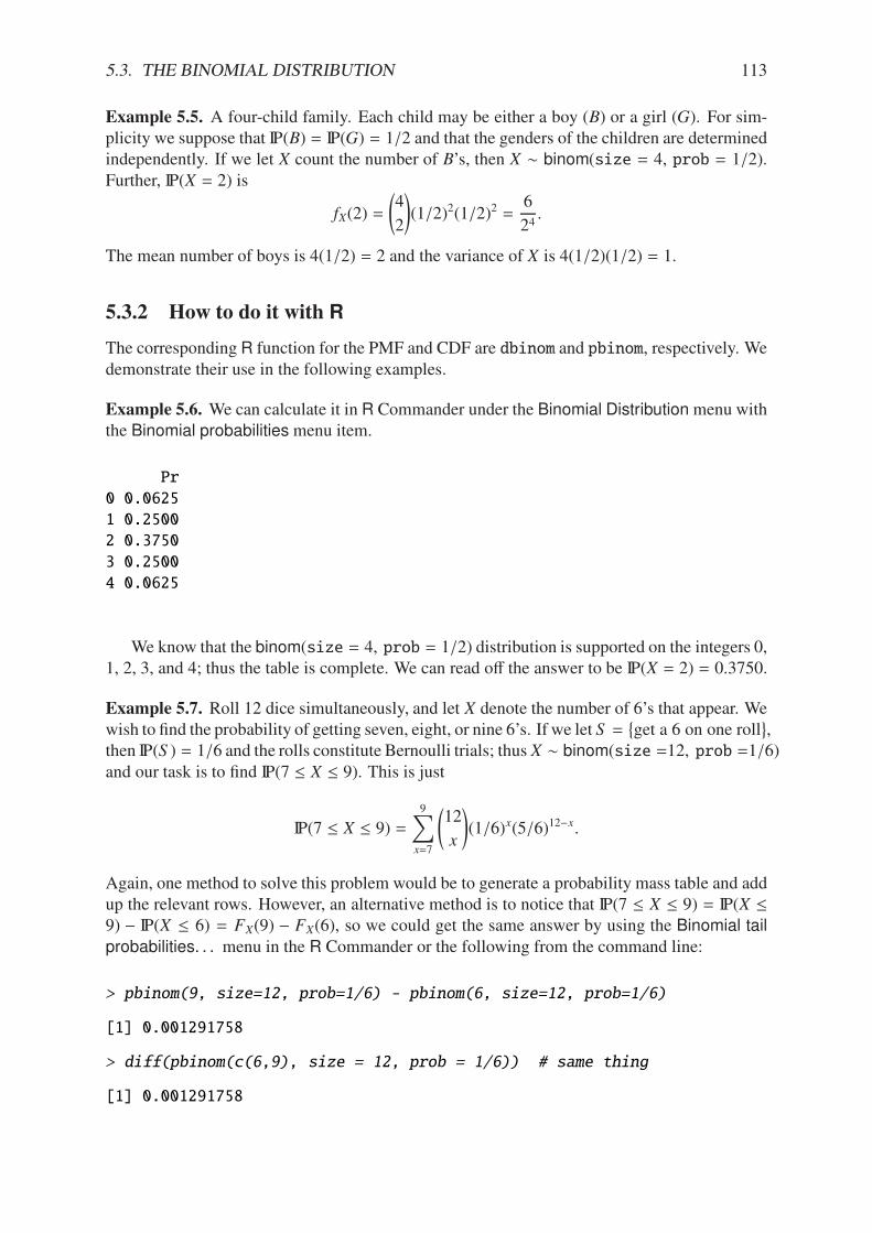
5.3. THE BINOMIAL DISTRIBUTION 113
Example 5.5. A four-child family. Each child may be either a boy (B) or a girl (G). For sim-plicity we suppose that IP(B) = IP(G) = 1/2 and that the genders of the children are determinedindependently. If we let X count the number of B’s, then X 4 binom(size = 4, prob = 1/2).Further, IP(X = 2) is
fX(2) =
04
2
1(1/2)2(1/2)2 =
6
24.
The mean number of boys is 4(1/2) = 2 and the variance of X is 4(1/2)(1/2) = 1.
5.3.2 How to do it with R
The corresponding R function for the PMF and CDF are dbinom and pbinom, respectively. Wedemonstrate their use in the following examples.
Example 5.6. We can calculate it in R Commander under the Binomial Distribution menu withthe Binomial probabilities menu item.
Pr
0 0.0625
1 0.2500
2 0.3750
3 0.2500
4 0.0625
We know that the binom(size = 4, prob = 1/2) distribution is supported on the integers 0,1, 2, 3, and 4; thus the table is complete. We can read o! the answer to be IP(X = 2) = 0.3750.
Example 5.7. Roll 12 dice simultaneously, and let X denote the number of 6’s that appear. Wewish to find the probability of getting seven, eight, or nine 6’s. If we let S =
,get a 6 on one roll
-,
then IP(S ) = 1/6 and the rolls constitute Bernoulli trials; thus X 4 binom(size =12, prob =1/6)and our task is to find IP(7 " X " 9). This is just
IP(7 " X " 9) =9!
x=7
012
x
1(1/6)x(5/6)12#x.
Again, one method to solve this problem would be to generate a probability mass table and addup the relevant rows. However, an alternative method is to notice that IP(7 " X " 9) = IP(X "9) # IP(X " 6) = FX(9) # FX(6), so we could get the same answer by using the Binomial tailprobabilities. . . menu in the R Commander or the following from the command line:
> pbinom(9, size=12, prob=1/6) - pbinom(6, size=12, prob=1/6)
[1] 0.001291758
> diff(pbinom(c(6,9), size = 12, prob = 1/6)) # same thing
[1] 0.001291758
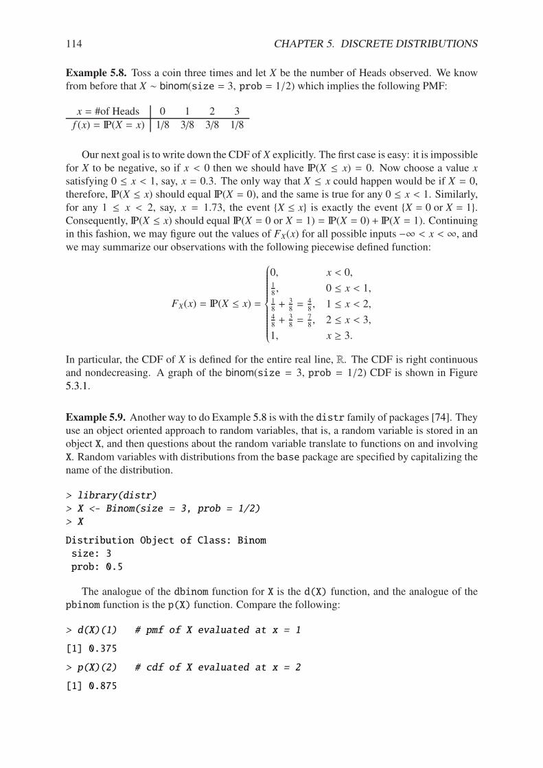
114 CHAPTER 5. DISCRETE DISTRIBUTIONS
Example 5.8. Toss a coin three times and let X be the number of Heads observed. We knowfrom before that X 4 binom(size = 3, prob = 1/2) which implies the following PMF:
x = #of Heads 0 1 2 3f (x) = IP(X = x) 1/8 3/8 3/8 1/8
Our next goal is to write down the CDF of X explicitly. The first case is easy: it is impossiblefor X to be negative, so if x < 0 then we should have IP(X " x) = 0. Now choose a value x
satisfying 0 " x < 1, say, x = 0.3. The only way that X " x could happen would be if X = 0,therefore, IP(X " x) should equal IP(X = 0), and the same is true for any 0 " x < 1. Similarly,for any 1 " x < 2, say, x = 1.73, the event {X " x} is exactly the event {X = 0 or X = 1}.Consequently, IP(X " x) should equal IP(X = 0 or X = 1) = IP(X = 0) + IP(X = 1). Continuingin this fashion, we may figure out the values of FX(x) for all possible inputs #& < x < &, andwe may summarize our observations with the following piecewise defined function:
FX(x) = IP(X " x) =
9:::::::::::;:::::::::::<
0, x < 0,18, 0 " x < 1,
18+ 3
8= 4
8, 1 " x < 2,
48+ 3
8= 7
8, 2 " x < 3,
1, x / 3.
In particular, the CDF of X is defined for the entire real line, R. The CDF is right continuousand nondecreasing. A graph of the binom(size = 3, prob = 1/2) CDF is shown in Figure5.3.1.
Example 5.9. Another way to do Example 5.8 is with the distr family of packages [74]. Theyuse an object oriented approach to random variables, that is, a random variable is stored in anobject X, and then questions about the random variable translate to functions on and involvingX. Random variables with distributions from the base package are specified by capitalizing thename of the distribution.
> library(distr)
> X <- Binom(size = 3, prob = 1/2)
> X
Distribution Object of Class: Binom
size: 3
prob: 0.5
The analogue of the dbinom function for X is the d(X) function, and the analogue of thepbinom function is the p(X) function. Compare the following:
> d(X)(1) # pmf of X evaluated at x = 1
[1] 0.375
> p(X)(2) # cdf of X evaluated at x = 2
[1] 0.875
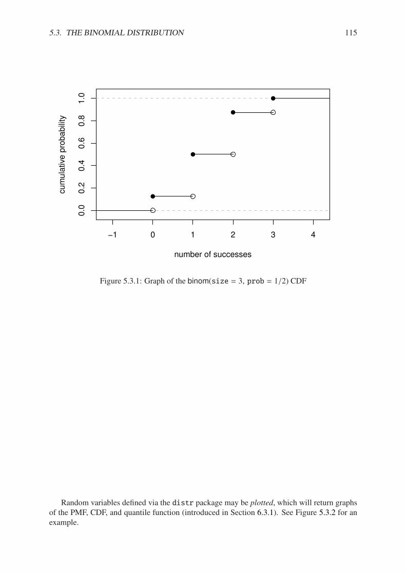
5.3. THE BINOMIAL DISTRIBUTION 115
!1 0 1 2 3 4
0.0
0.2
0.4
0.6
0.8
1.0
number of successes
cum
ula
tive p
robabili
ty
Figure 5.3.1: Graph of the binom(size = 3, prob = 1/2) CDF
Random variables defined via the distr package may be plotted, which will return graphsof the PMF, CDF, and quantile function (introduced in Section 6.3.1). See Figure 5.3.2 for anexample.
116 CHAPTER 5. DISCRETE DISTRIBUTIONS
Given X 4 dbinom(size = n, prob = p).
How to do: with stats (default) with distrPMF: IP(X = x) dbinom(x, size = n, prob = p) d(X)(x)CDF: IP(X " x) pbinom(x, size = n, prob = p) p(X)(x)Simulate k variates rbinom(k, size = n, prob = p) r(X)(k)
For distr need X <- Binom(size =n, prob =p)
Table 5.1: Correspondence between stats and distr
0.0 1.0 2.0 3.0
0.0
0.1
0.2
0.3
x
d(x
)
Probability function of Binom(3, 0.5)
!1 0 1 2 3 4
0.0
0.2
0.4
0.6
0.8
1.0
q
p(q
)
CDF of Binom(3, 0.5)
0.0 0.4 0.8
0.0
0.5
1.0
1.5
2.0
2.5
3.0
p
q(p
)
Quantile function of Binom(3, 0.5)
Figure 5.3.2: The binom(size = 3, prob = 0.5) distribution from the distr package
5.4 Expectation and Moment Generating Functions
5.4.1 The Expectation Operator
We next generalize some of the concepts from Section 5.1.2. There we saw that every1 PMFhas two important numbers associated with it:
µ =!
x3S
x fX(x), "2 =
!
x3S
(x # µ)2 fX(x). (5.4.1)
Intuitively, for repeated observations of X we would expect the sample mean to closely approx-imate µ as the sample size increases without bound. For this reason we call µ the expected
value of X and we write µ = IE X, where IE is an expectation operator.
1Not every, only those PMFs for which the (potentially infinite) series converges.

5.4. EXPECTATION AND MOMENT GENERATING FUNCTIONS 117
Definition 5.10. More generally, given a function g we define the expected value of g(X) by
IE g(X) =!
x3S
g(x) fX(x), (5.4.2)
provided the (potentially infinite) series#
x |g(x)| f (x) is convergent. We say that IE g(X) exists.
In this notation the variance is "2 = IE(X # µ)2 and we prove the identity
IE(X # µ)2 = IE X2 # (IE X)2 (5.4.3)
in Exercise 5.4. Intuitively, for repeated observations of X we would expect the sample meanof the g(X) values to closely approximate IE g(X) as the sample size increases without bound.
Let us take the analogy further. If we expect g(X) to be close to IE g(X) on the average,where would we expect 3g(X) to be on the average? It could only be 3 IE g(X). The followingtheorem makes this idea precise.
Proposition 5.11. For any functions g and h, any random variable X, and any constant c:
1. IE c = c,
2. IE[c · g(X)] = c IE g(X)
3. IE[g(X) + h(X)] = IE g(X) + IE h(X),
provided IE g(X) and IE h(X) exist.
Proof. Go directly from the definition. For example,
IE[c · g(X)] =!
x3S
c · g(x) fX(x) = c ·!
x3S
g(x) fX(x) = c IE g(X).
"
5.4.2 Moment Generating Functions
Definition 5.12. Given a random variable X, its moment generating function (abbreviatedMGF) is defined by the formula
MX(t) = IE etX =!
x3S
etx fX(x), (5.4.4)
provided the (potentially infinite) series is convergent for all t in a neighborhood of zero (thatis, for all #$ < t < $, for some $ > 0).
Note that for any MGF MX,
MX(0) = IE e0·X = IE 1 = 1. (5.4.5)
We will calculate the MGF for the two distributions introduced above.
Example 5.13. Find the MGF for X 4 disunif(m).Since f (x) = 1/m, the MGF takes the form
M(t) =m!
x=1
etx1
m=
1
m(et + e2t + · · · + emt), for any t.
118 CHAPTER 5. DISCRETE DISTRIBUTIONS
Example 5.14. Find the MGF for X 4 binom(size = n, prob = p).
MX(t) =n!
x=0
etx0n
x
1px(1 # p)n#x,
=
n#x!
x=0
0n
x
1(pet)xqn#x,
=(pet + q)n, for any t.
Applications
We will discuss three applications of moment generating functions in this book. The first is thefact that an MGF may be used to accurately identify the probability distribution that generatedit, which rests on the following:
Theorem 5.15. The moment generating function, if it exists in a neighborhood of zero, deter-
mines a probability distribution uniquely.
Proof. Unfortunately, the proof of such a theorem is beyond the scope of a text like this one.Interested readers could consult Billingsley [8]. "
We will see an example of Theorem 5.15 in action.
Example 5.16. Suppose we encounter a random variable which has MGF
MX(t) = (0.3 + 0.7et)13.
Then X 4 binom(size = 13, prob = 0.7).
An MGF is also known as a “Laplace Transform” and is manipulated in that context inmany branches of science and engineering.
Why is it called a Moment Generating Function?
This brings us to the second powerful application of MGFs. Many of the models we studyhave a simple MGF, indeed, which permits us to determine the mean, variance, and even highermoments very quickly. Let us see why. We already know that
M(t) =!
x3S
etx f (x).
Take the derivative with respect to t to get
M5(t) =d
dt
$%%%%%&!
x3S
etx f (x)
()))))* =
!
x3S
d
dt
=etx f (x)
>=
!
x3S
xetx f (x), (5.4.6)
and so if we plug in zero for t we see
M5(0) =!
x3S
xe0 f (x) =!
x3S
x f (x) = µ = IE X. (5.4.7)
5.4. EXPECTATION AND MOMENT GENERATING FUNCTIONS 119
Similarly, M55(t) =#
x2etx f (x) so that M55(0) = IE X2. And in general, we can see2 that
M(r)X (0) = IE Xr = rthmoment of Xabout the origin. (5.4.8)
These are also known as raw moments and are sometimes denoted µ5r. In addition to these arethe so called central moments µr defined by
µr = IE(X # µ)r, r = 1, 2, . . . (5.4.9)
Example 5.17. Let X 4 binom(size = n, prob = p) with M(t) = (q + pet)n. We calculatedthe mean and variance of a binomial random variable in Section 5.3 by means of the binomialseries. But look how quickly we find the mean and variance with the moment generatingfunction.
M5(t) =n(q + pet)n#1pet |t=0 ,
=n · 1n#1p,=np.
And
M55(0) =n(n # 1)[q + pet]n#2(pet)2 + n[q + pet]n#1pet |t=0 ,
IE X2 =n(n # 1)p2 + np.
Therefore
"2 = IE X2 # (IE X)2,
=n(n # 1)p2 + np # n2p2,
=np # np2 = npq.
See how much easier that was?
Remark 5.18. We learned in this section that M(r)(0) = IE Xr. We remember from Calculus IIthat certain functions f can be represented by a Taylor series expansion about a point a, whichtakes the form
f (x) =&!
r=0
f (r)(a)
r!(x # a)r, for all |x # a| < R, (5.4.10)
where R is called the radius of convergence of the series (see Appendix E.3). We combine thetwo to say that if an MGF exists for all t in the interval (#$, $), then we can write
MX(t) =&!
r=0
IE Xr
r!tr, for all |t| < $. (5.4.11)
2We are glossing over some significant mathematical details in our derivation. Su"ce it to say that when theMGF exists in a neighborhood of t = 0, the exchange of di!erentiation and summation is valid in that neighbor-hood, and our remarks hold true.
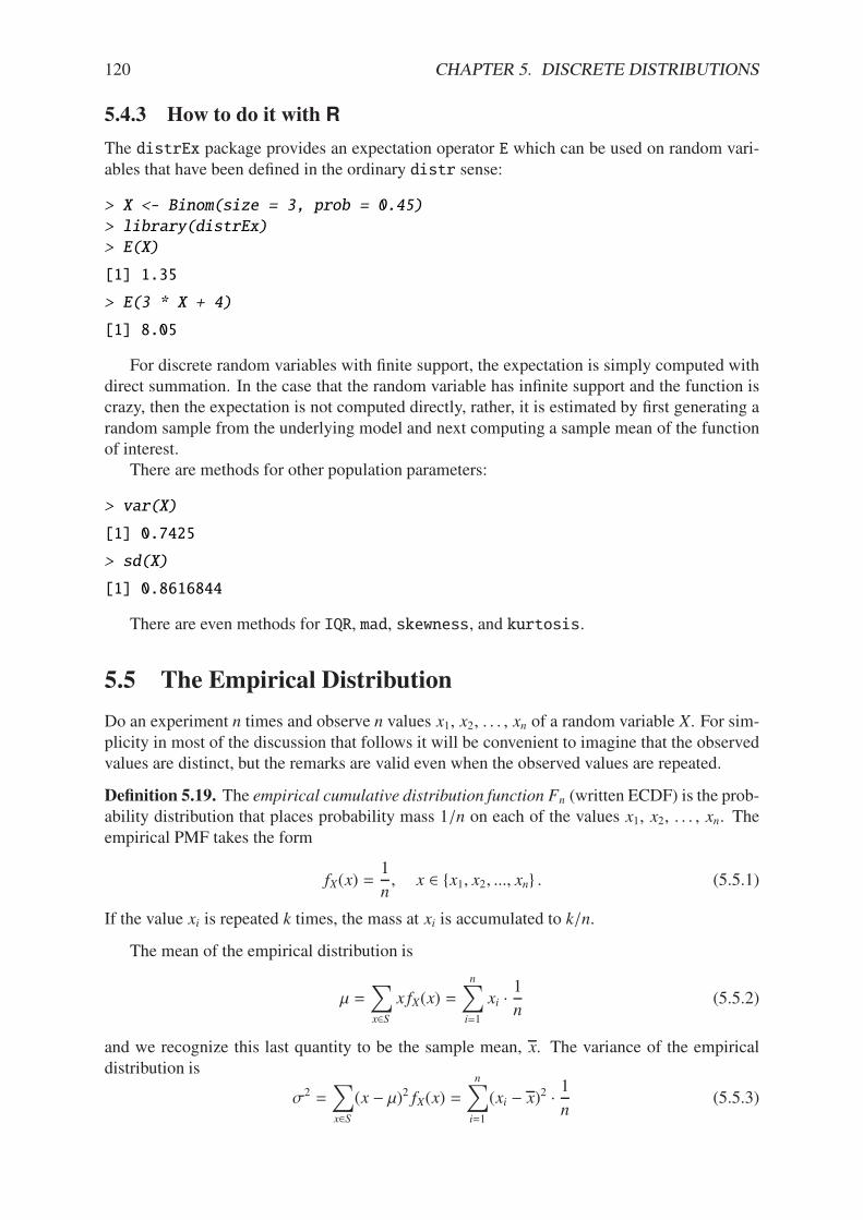
120 CHAPTER 5. DISCRETE DISTRIBUTIONS
5.4.3 How to do it with R
The distrEx package provides an expectation operator E which can be used on random vari-ables that have been defined in the ordinary distr sense:
> X <- Binom(size = 3, prob = 0.45)
> library(distrEx)
> E(X)
[1] 1.35
> E(3 * X + 4)
[1] 8.05
For discrete random variables with finite support, the expectation is simply computed withdirect summation. In the case that the random variable has infinite support and the function iscrazy, then the expectation is not computed directly, rather, it is estimated by first generating arandom sample from the underlying model and next computing a sample mean of the functionof interest.
There are methods for other population parameters:
> var(X)
[1] 0.7425
> sd(X)
[1] 0.8616844
There are even methods for IQR, mad, skewness, and kurtosis.
5.5 The Empirical Distribution
Do an experiment n times and observe n values x1, x2, . . . , xn of a random variable X. For sim-plicity in most of the discussion that follows it will be convenient to imagine that the observedvalues are distinct, but the remarks are valid even when the observed values are repeated.
Definition 5.19. The empirical cumulative distribution function Fn (written ECDF) is the prob-ability distribution that places probability mass 1/n on each of the values x1, x2, . . . , xn. Theempirical PMF takes the form
fX(x) =1
n, x 3 {x1, x2, ..., xn} . (5.5.1)
If the value xi is repeated k times, the mass at xi is accumulated to k/n.
The mean of the empirical distribution is
µ =!
x3S
x fX(x) =n!
i=1
xi ·1
n(5.5.2)
and we recognize this last quantity to be the sample mean, x. The variance of the empiricaldistribution is
"2 =!
x3S
(x # µ)2 fX(x) =n!
i=1
(xi # x)2 ·1
n(5.5.3)

5.5. THE EMPIRICAL DISTRIBUTION 121
and this last quantity looks very close to what we already know to be the sample variance.
s2 =1
n # 1
n!
i=1
(xi # x)2. (5.5.4)
The empirical quantile function is the inverse of the ECDF. See Section 6.3.1.
5.5.1 How to do it with R
The empirical distribution is not directly available as a distribution in the same way that theother base probability distributions are, but there are plenty of resources available for the deter-mined investigator.
Given a data vector of observed values x, we can see the empirical CDF with the ecdffunction:
> x <- c(4, 7, 9, 11, 12)
> ecdf(x)
Empirical CDF
Call: ecdf(x)
x[1:5] = 4, 7, 9, 11, 12
The above shows that the returned value of ecdf(x) is not a number but rather a function.The ECDF is not usually used by itself in this form, by itself. More commonly it is used asan intermediate step in a more complicated calculation, for instance, in hypothesis testing (seeChapter 10) or resampling (see Chapter 13). It is nevertheless instructive to see what the ecdflooks like, and there is a special plot method for ecdf objects.
> plot(ecdf(x))
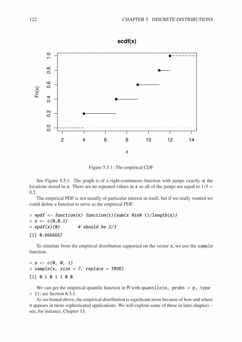
122 CHAPTER 5. DISCRETE DISTRIBUTIONS
2 4 6 8 10 12 14
0.0
0.2
0.4
0.6
0.8
1.0
ecdf(x)
x
Fn(x
)
Figure 5.5.1: The empirical CDF
See Figure 5.5.1. The graph is of a right-continuous function with jumps exactly at thelocations stored in x. There are no repeated values in x so all of the jumps are equal to 1/5 =0.2.
The empirical PDF is not usually of particular interest in itself, but if we really wanted wecould define a function to serve as the empirical PDF:
> epdf <- function(x) function(t){sum(x %in% t)/length(x)}
> x <- c(0,0,1)
> epdf(x)(0) # should be 2/3
[1] 0.6666667
To simulate from the empirical distribution supported on the vector x, we use the samplefunction.
> x <- c(0, 0, 1)
> sample(x, size = 7, replace = TRUE)
[1] 0 1 0 1 1 0 0
We can get the empirical quantile function in R with quantile(x, probs = p, type= 1); see Section 6.3.1.
As we hinted above, the empirical distribution is significant more because of how and whereit appears in more sophisticated applications. We will explore some of these in later chapters –see, for instance, Chapter 13.
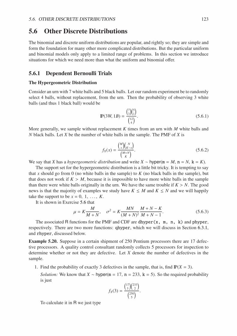
5.6. OTHER DISCRETE DISTRIBUTIONS 123
5.6 Other Discrete Distributions
The binomial and discrete uniform distributions are popular, and rightly so; they are simple andform the foundation for many other more complicated distributions. But the particular uniformand binomial models only apply to a limited range of problems. In this section we introducesituations for which we need more than what the uniform and binomial o!er.
5.6.1 Dependent Bernoulli Trials
The Hypergeometric Distribution
Consider an urn with 7 white balls and 5 black balls. Let our random experiment be to randomlyselect 4 balls, without replacement, from the urn. Then the probability of observing 3 whiteballs (and thus 1 black ball) would be
IP(3W, 1B) =
273
3251
3
2124
3 . (5.6.1)
More generally, we sample without replacement K times from an urn with M white balls andN black balls. Let X be the number of white balls in the sample. The PMF of X is
fX(x) =
2Mx
32N
K#x
3
2M+NK
3 . (5.6.2)
We say that X has a hypergeometric distribution and write X 4 hyper(m = M, n = N, k = K).The support set for the hypergeometric distribution is a little bit tricky. It is tempting to say
that x should go from 0 (no white balls in the sample) to K (no black balls in the sample), butthat does not work if K > M, because it is impossible to have more white balls in the samplethan there were white balls originally in the urn. We have the same trouble if K > N. The goodnews is that the majority of examples we study have K " M and K " N and we will happilytake the support to be x = 0, 1, . . . , K.
It is shown in Exercise 5.6 that
µ = KM
M + N, "2 = K
MN
(M + N)2M + N # K
M + N # 1. (5.6.3)
The associated R functions for the PMF and CDF are dhyper(x, m, n, k) and phyper,respectively. There are two more functions: qhyper, which we will discuss in Section 6.3.1,and rhyper, discussed below.
Example 5.20. Suppose in a certain shipment of 250 Pentium processors there are 17 defec-tive processors. A quality control consultant randomly collects 5 processors for inspection todetermine whether or not they are defective. Let X denote the number of defectives in thesample.
1. Find the probability of exactly 3 defectives in the sample, that is, find IP(X = 3).
Solution: We know that X 4 hyper(m = 17, n = 233, k = 5). So the required probabilityis just
fX(3) =
2173
322332
3
22505
3 .
To calculate it in R we just type
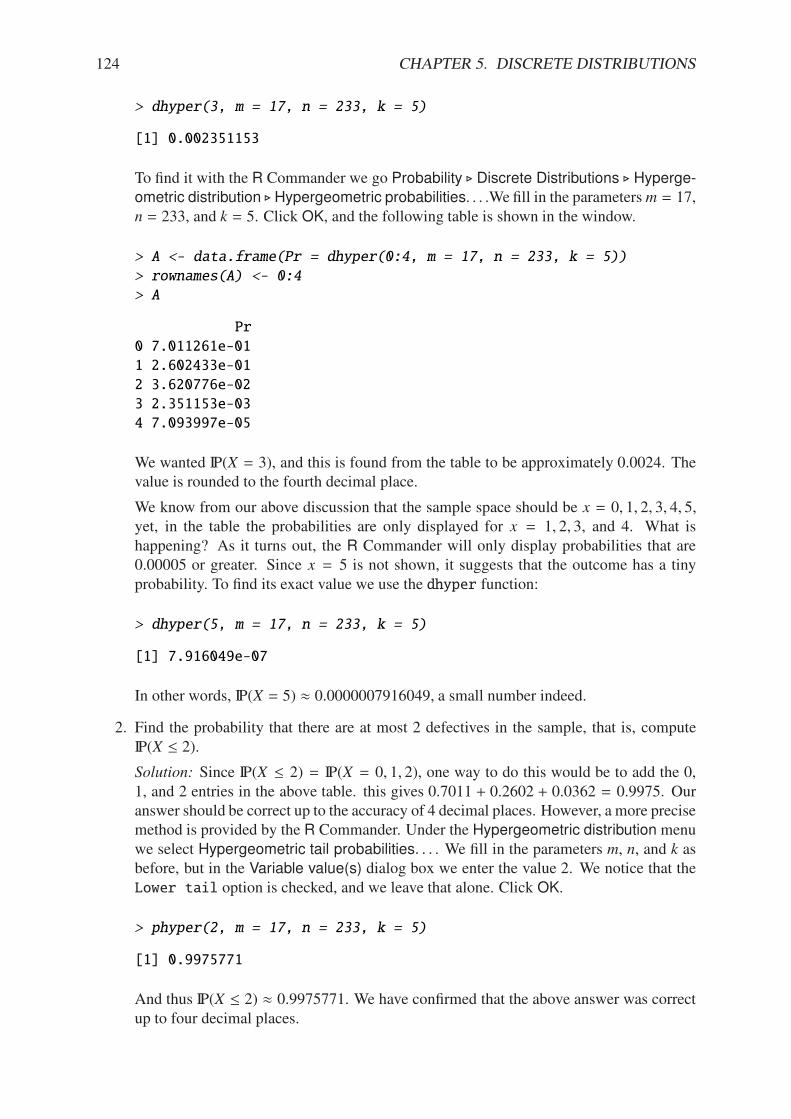
124 CHAPTER 5. DISCRETE DISTRIBUTIONS
> dhyper(3, m = 17, n = 233, k = 5)
[1] 0.002351153
To find it with the R Commander we go Probability ! Discrete Distributions ! Hyperge-ometric distribution ! Hypergeometric probabilities. . . .We fill in the parametersm = 17,n = 233, and k = 5. Click OK, and the following table is shown in the window.
> A <- data.frame(Pr = dhyper(0:4, m = 17, n = 233, k = 5))
> rownames(A) <- 0:4
> A
Pr
0 7.011261e-01
1 2.602433e-01
2 3.620776e-02
3 2.351153e-03
4 7.093997e-05
We wanted IP(X = 3), and this is found from the table to be approximately 0.0024. Thevalue is rounded to the fourth decimal place.
We know from our above discussion that the sample space should be x = 0, 1, 2, 3, 4, 5,yet, in the table the probabilities are only displayed for x = 1, 2, 3, and 4. What ishappening? As it turns out, the R Commander will only display probabilities that are0.00005 or greater. Since x = 5 is not shown, it suggests that the outcome has a tinyprobability. To find its exact value we use the dhyper function:
> dhyper(5, m = 17, n = 233, k = 5)
[1] 7.916049e-07
In other words, IP(X = 5) ' 0.0000007916049, a small number indeed.
2. Find the probability that there are at most 2 defectives in the sample, that is, computeIP(X " 2).
Solution: Since IP(X " 2) = IP(X = 0, 1, 2), one way to do this would be to add the 0,1, and 2 entries in the above table. this gives 0.7011 + 0.2602 + 0.0362 = 0.9975. Ouranswer should be correct up to the accuracy of 4 decimal places. However, a more precisemethod is provided by the R Commander. Under the Hypergeometric distribution menuwe select Hypergeometric tail probabilities. . . . We fill in the parameters m, n, and k asbefore, but in the Variable value(s) dialog box we enter the value 2. We notice that theLower tail option is checked, and we leave that alone. Click OK.
> phyper(2, m = 17, n = 233, k = 5)
[1] 0.9975771
And thus IP(X " 2) ' 0.9975771. We have confirmed that the above answer was correctup to four decimal places.
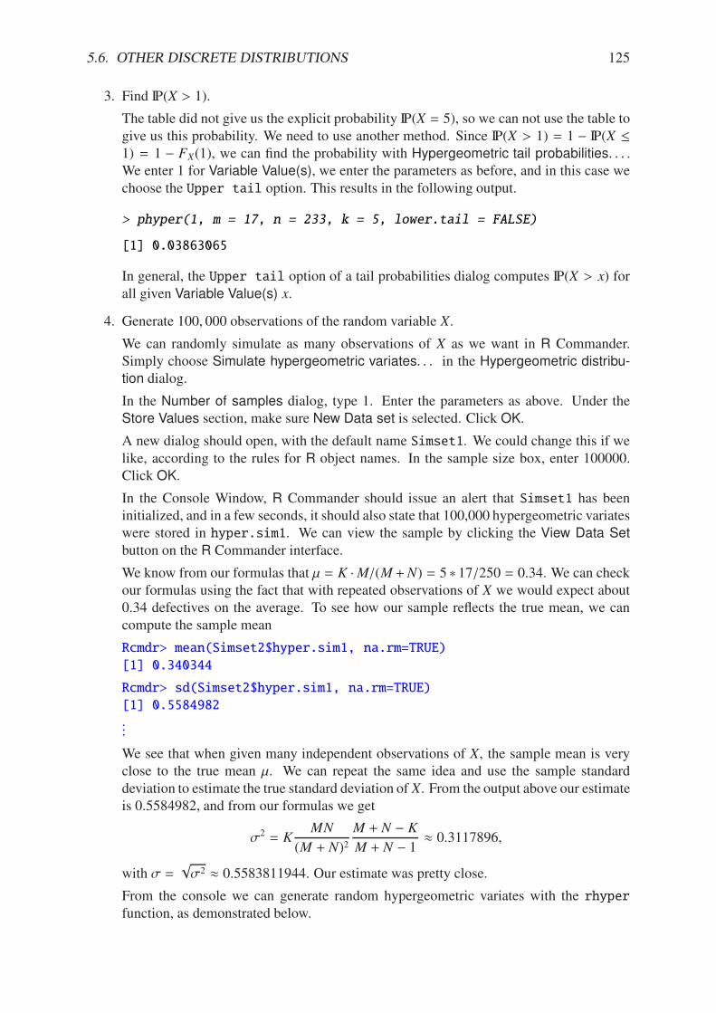
5.6. OTHER DISCRETE DISTRIBUTIONS 125
3. Find IP(X > 1).
The table did not give us the explicit probability IP(X = 5), so we can not use the table togive us this probability. We need to use another method. Since IP(X > 1) = 1 # IP(X "1) = 1 # FX(1), we can find the probability with Hypergeometric tail probabilities. . . .We enter 1 for Variable Value(s), we enter the parameters as before, and in this case wechoose the Upper tail option. This results in the following output.
> phyper(1, m = 17, n = 233, k = 5, lower.tail = FALSE)
[1] 0.03863065
In general, the Upper tail option of a tail probabilities dialog computes IP(X > x) forall given Variable Value(s) x.
4. Generate 100, 000 observations of the random variable X.
We can randomly simulate as many observations of X as we want in R Commander.Simply choose Simulate hypergeometric variates. . . in the Hypergeometric distribu-tion dialog.
In the Number of samples dialog, type 1. Enter the parameters as above. Under theStore Values section, make sure New Data set is selected. Click OK.
A new dialog should open, with the default name Simset1. We could change this if welike, according to the rules for R object names. In the sample size box, enter 100000.Click OK.
In the Console Window, R Commander should issue an alert that Simset1 has beeninitialized, and in a few seconds, it should also state that 100,000 hypergeometric variateswere stored in hyper.sim1. We can view the sample by clicking the View Data Setbutton on the R Commander interface.
We know from our formulas that µ = K ·M/(M +N) = 5 6 17/250 = 0.34. We can checkour formulas using the fact that with repeated observations of X we would expect about0.34 defectives on the average. To see how our sample reflects the true mean, we cancompute the sample mean
Rcmdr> mean(Simset2$hyper.sim1, na.rm=TRUE)
[1] 0.340344
Rcmdr> sd(Simset2$hyper.sim1, na.rm=TRUE)
[1] 0.5584982
...
We see that when given many independent observations of X, the sample mean is veryclose to the true mean µ. We can repeat the same idea and use the sample standarddeviation to estimate the true standard deviation of X. From the output above our estimateis 0.5584982, and from our formulas we get
"2 = KMN
(M + N)2M + N # K
M + N # 1' 0.3117896,
with " =$"2 ' 0.5583811944. Our estimate was pretty close.
From the console we can generate random hypergeometric variates with the rhyperfunction, as demonstrated below.
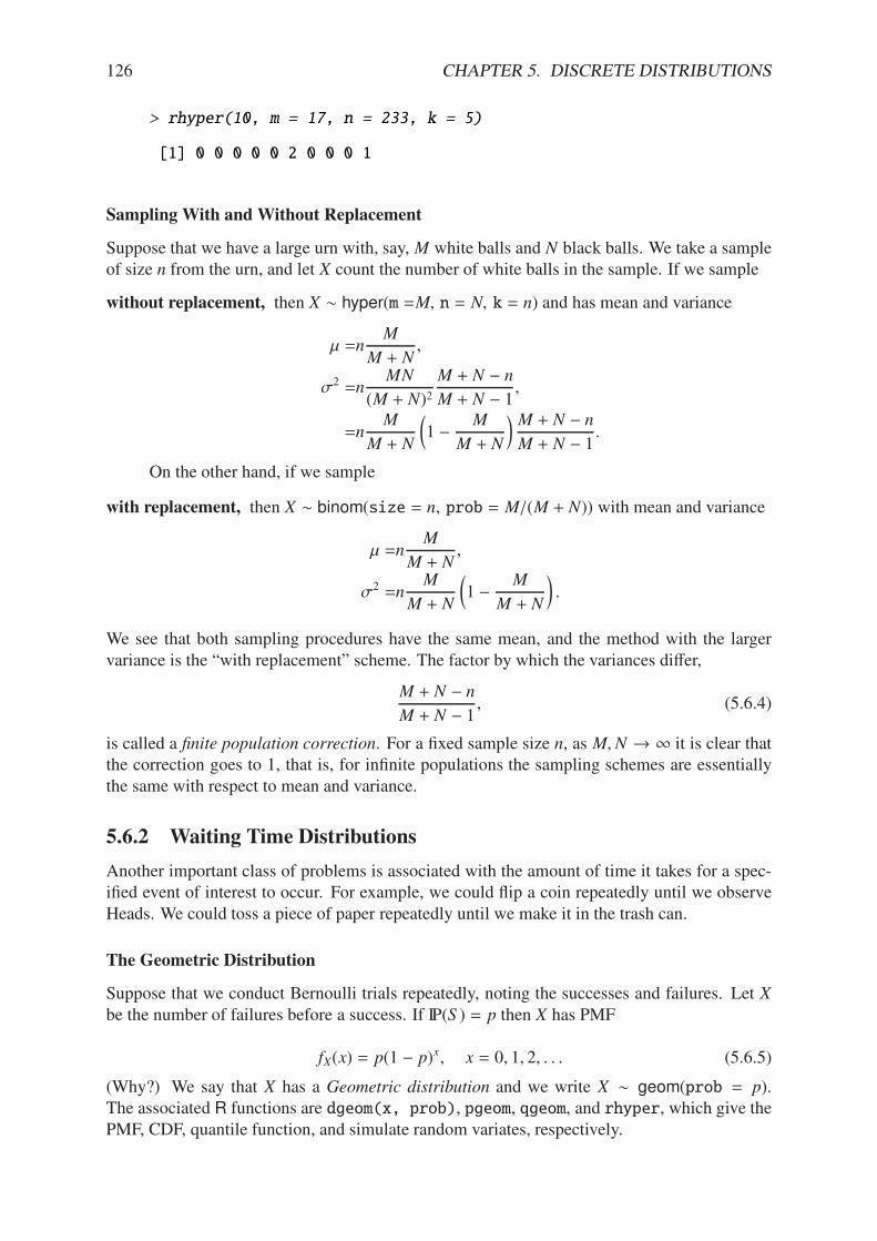
126 CHAPTER 5. DISCRETE DISTRIBUTIONS
> rhyper(10, m = 17, n = 233, k = 5)
[1] 0 0 0 0 0 2 0 0 0 1
Sampling With and Without Replacement
Suppose that we have a large urn with, say, M white balls and N black balls. We take a sampleof size n from the urn, and let X count the number of white balls in the sample. If we sample
without replacement, then X 4 hyper(m =M, n = N, k = n) and has mean and variance
µ =nM
M + N,
"2 =nMN
(M + N)2M + N # n
M + N # 1,
=nM
M + N
?1 #
M
M + N
@M + N # n
M + N # 1.
On the other hand, if we sample
with replacement, then X 4 binom(size = n, prob = M/(M + N)) with mean and variance
µ =nM
M + N,
"2 =nM
M + N
?1 #
M
M + N
@.
We see that both sampling procedures have the same mean, and the method with the largervariance is the “with replacement” scheme. The factor by which the variances di!er,
M + N # n
M + N # 1, (5.6.4)
is called a finite population correction. For a fixed sample size n, as M,N . & it is clear thatthe correction goes to 1, that is, for infinite populations the sampling schemes are essentiallythe same with respect to mean and variance.
5.6.2 Waiting Time Distributions
Another important class of problems is associated with the amount of time it takes for a spec-ified event of interest to occur. For example, we could flip a coin repeatedly until we observeHeads. We could toss a piece of paper repeatedly until we make it in the trash can.
The Geometric Distribution
Suppose that we conduct Bernoulli trials repeatedly, noting the successes and failures. Let Xbe the number of failures before a success. If IP(S ) = p then X has PMF
fX(x) = p(1 # p)x, x = 0, 1, 2, . . . (5.6.5)
(Why?) We say that X has a Geometric distribution and we write X 4 geom(prob = p).The associated R functions are dgeom(x, prob), pgeom, qgeom, and rhyper, which give thePMF, CDF, quantile function, and simulate random variates, respectively.
5.6. OTHER DISCRETE DISTRIBUTIONS 127
Again it is clear that f (x) / 0 and we check that#
f (x) = 1 (see Equation E.3.9 in Ap-pendix E.3):
&!
x=0
p(1 # p)x =p&!
x=0
qx = p1
1 # q= 1.
We will find in the next section that the mean and variance are
µ =1 # p
p=
q
pand "2 =
q
p2. (5.6.6)
Example 5.21. The Pittsburgh Steelers place kicker, Je! Reed, made 81.2% of his attemptedfield goals in his career up to 2006. Assuming that his successive field goal attempts are ap-proximately Bernoulli trials, find the probability that Je!misses at least 5 field goals before hisfirst successful goal.
Solution: If X = the number of missed goals until Je!’s first success, then X 4 geom(prob =0.812) and we want IP(X / 5) = IP(X > 4). We can find this in R with
> pgeom(4, prob = 0.812, lower.tail = FALSE)
[1] 0.0002348493
Note 5.22. Some books use a slightly di!erent definition of the geometric distribution. Theyconsider Bernoulli trials and let Y count instead the number of trials until a success, so that Yhas PMF
fY(y) = p(1 # p)y#1, y = 1, 2, 3, . . . (5.6.7)
When they say “geometric distribution”, this is what they mean. It is not hard to see that thetwo definitions are related. In fact, if X denotes our geometric and Y theirs, then Y = X + 1.Consequently, they have µY = µX + 1 and "2
Y = "2X.
The Negative Binomial Distribution
We may generalize the problem and consider the case where we wait for more than one suc-cess. Suppose that we conduct Bernoulli trials repeatedly, noting the respective successes andfailures. Let X count the number of failures before r successes. If IP(S ) = p then X has PMF
fX(x) =
0r + x # 1
r # 1
1pr(1 # p)x, x = 0, 1, 2, . . . (5.6.8)
We say that X has a Negative Binomial distribution and write X 4 nbinom(size = r, prob =
p). The associated R functions are dnbinom(x, size, prob), pnbinom, qnbinom, andrnbinom, which give the PMF, CDF, quantile function, and simulate random variates, respec-tively.
As usual it should be clear that fX(x) / 0 and the fact that#
fX(x) = 1 follows from ageneralization of the geometric series by means of a Maclaurin’s series expansion:
1
1 # t=
&!
k=0
tk, for #1 < t < 1, and (5.6.9)
1
(1 # t)r=
&!
k=0
0r + k # 1
r # 1
1tk, for #1 < t < 1. (5.6.10)
128 CHAPTER 5. DISCRETE DISTRIBUTIONS
Therefore&!
x=0
fX(x) = pr&!
x=0
0r + x # 1
r # 1
1qx = pr(1 # q)#r = 1, (5.6.11)
since |q| = |1 # p| < 1.
Example 5.23. We flip a coin repeatedly and let X count the number of Tails until we get sevenHeads. What is IP(X = 5)?
Solution: We know that X 4 nbinom(size = 7, prob = 1/2).
IP(X = 5) = fX(5) =
07 + 5 # 1
7 # 1
1(1/2)7(1/2)5 =
011
6
12#12
and we can get this in R with
> dnbinom(5, size = 7, prob = 0.5)
[1] 0.1127930
Let us next compute the MGF of X 4 nbinom(size = r, prob = p).
MX(t) =&!
x=0
etx0r + x # 1
r # 1
1prqx
=pr&!
x=0
0r + x # 1
r # 1
1[qet]x
=pr(1 # qet)#r, provided |qet| < 1,
and so
MX(t) =
0p
1 # qet
1r, for qet < 1. (5.6.12)
We see that qet < 1 when t < # ln(1 # p).Let X 4 nbinom(size = r, prob = p) with M(t) = pr(1 # qet)#r. We proclaimed above the
values of the mean and variance. Now we are equipped with the tools to find these directly.
M5(t) =pr(#r)(1 # qet)#r#1(#qet),
=rqet pr(1 # qet)#r#1,
=rqet
1 # qetM(t), and so
M5(0) =rq
1 # q· 1 =
rq
p.
Thus µ = rq/p. We next find IE X2.
M55(0) =rqet(1 # qet) # rqet(#qet)
(1 # qet)2M(t) +
rqet
1 # qetM5(t)
44444t=0
,
=rqp + rq2
p2· 1 +
rq
p
0rq
p
1,
=rq
p2+
0rq
p
12.
Finally we may say "2 = M55(0) # [M5(0)]2 = rq/p2.
5.6. OTHER DISCRETE DISTRIBUTIONS 129
Example 5.24. A random variable has MGF
MX(t) =
00.19
1 # 0.81et
131.
Then X 4 nbinom(size = 31, prob = 0.19).
Note 5.25. As with the Geometric distribution, some books use a slightly di!erent definition ofthe Negative Binomial distribution. They consider Bernoulli trials and let Y be the number oftrials until r successes, so that Y has PMF
fY(y) =
0y # 1
r # 1
1pr(1 # p)y#r, y = r, r + 1, r + 2, . . . (5.6.13)
It is again not hard to see that if X denotes our Negative Binomial and Y theirs, then Y = X + r.Consequently, they have µY = µX + r and "
2Y = "
2X.
5.6.3 Arrival Processes
The Poisson Distribution
This is a distribution associated with “rare events”, for reasons which will become clear in amoment. The events might be:
• tra"c accidents,
• typing errors, or
• customers arriving in a bank.
Let % be the average number of events in the time interval [0, 1]. Let the random variable X
count the number of events occurring in the interval. Then under certain reasonable conditionsit can be shown that
fX(x) = IP(X = x) = e#%%x
x!, x = 0, 1, 2, . . . (5.6.14)
We use the notation X 4 pois(lambda = %). The associated R functions are dpois(x,lambda), ppois, qpois, and rpois, which give the PMF, CDF, quantile function, and simu-late random variates, respectively.
What are the reasonable conditions? Divide [0, 1] into subintervals of length 1/n. A Pois-
son process satisfies the following conditions:
• the probability of an event occurring in a particular subinterval is ' %/n.
• the probability of two or more events occurring in any subinterval is ' 0.
• occurrences in disjoint subintervals are independent.
Remark 5.26. If X counts the number of events in the interval [0, t] and % is the average numberthat occur in unit time, then X 4 pois(lambda = %t), that is,
IP(X = x) = e#%t(%t)x
x!, x = 0, 1, 2, 3 . . . (5.6.15)
130 CHAPTER 5. DISCRETE DISTRIBUTIONS
Example 5.27. On the average, five cars arrive at a particular car wash every hour. Let X countthe number of cars that arrive from 10AM to 11AM. Then X 4 pois(lambda = 5). Also,µ = "2 = 5. What is the probability that no car arrives during this period?
Solution: The probability that no car arrives is
IP(X = 0) = e#550
0!= e#5 ' 0.0067.
Example 5.28. Suppose the car wash above is in operation from 8AM to 6PM, and we let Y bethe number of customers that appear in this period. Since this period covers a total of 10 hours,from Remark 5.26 we get that Y 4 pois(lambda = 5 6 10 = 50). What is the probability thatthere are between 48 and 50 customers, inclusive?
Solution: We want IP(48 " Y " 50) = IP(X " 50) # IP(X " 47).
> diff(ppois(c(47, 50), lambda = 50))
[1] 0.1678485
5.7 Functions of Discrete Random Variables
We have built a large catalogue of discrete distributions, but the tools of this section will giveus the ability to consider infinitely many more. Given a random variable X and a given functionh, we may consider Y = h(X). Since the values of X are determined by chance, so are thevalues of Y . The question is, what is the PMF of the random variable Y? The answer, of course,depends on h. In the case that h is one-to-one (see Appendix E.2), the solution can be found bysimple substitution.
Example 5.29. Let X 4 nbinom(size = r, prob = p). We saw in 5.6 that X represents thenumber of failures until r successes in a sequence of Bernoulli trials. Suppose now that insteadwe were interested in counting the number of trials (successes and failures) until the rth successoccurs, which we will denote by Y . In a given performance of the experiment, the number offailures (X) and the number of successes (r) together will comprise the total number of trials(Y), or in other words, X+ r = Y . We may let h be defined by h(x) = x+ r so that Y = h(X), andwe notice that h is linear and hence one-to-one. Finally, X takes values 0, 1, 2, . . . implyingthat the support of Y would be {r, r + 1, r + 2, . . .}. Solving for X we get X = Y # r. Examiningthe PMF of X
fX(x) =
0r + x # 1
r # 1
1pr(1 # p)x, (5.7.1)
we can substitute x = y # r to get
fY(y) = fX(y # r),
=
0r + (y # r) # 1
r # 1
1pr(1 # p)y#r,
=
0y # 1
r # 1
1pr(1 # p)y#r, y = r, r + 1, . . .
Even when the function h is not one-to-one, we may still find the PMF of Y simply byaccumulating, for each y, the probability of all the x’s that are mapped to that y.
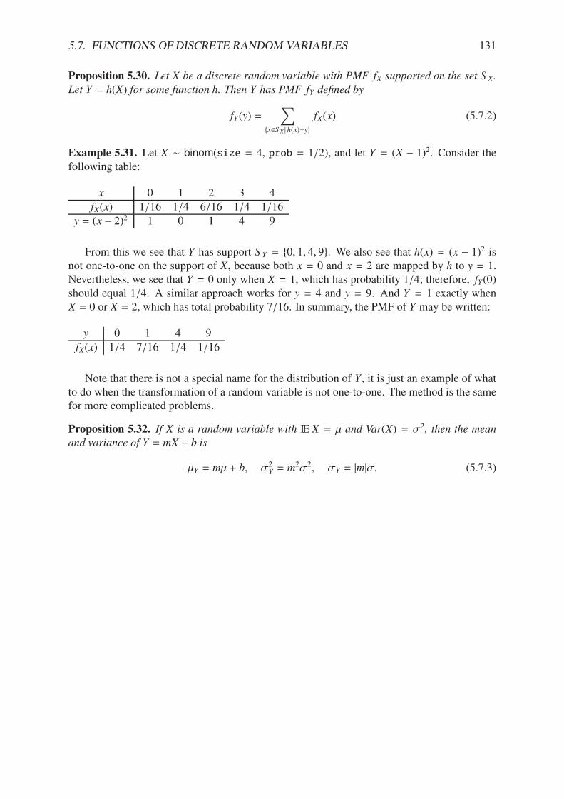
5.7. FUNCTIONS OF DISCRETE RANDOM VARIABLES 131
Proposition 5.30. Let X be a discrete random variable with PMF fX supported on the set S X.
Let Y = h(X) for some function h. Then Y has PMF fY defined by
fY(y) =!
{x3S X | h(x)=y}
fX(x) (5.7.2)
Example 5.31. Let X 4 binom(size = 4, prob = 1/2), and let Y = (X # 1)2. Consider thefollowing table:
x 0 1 2 3 4fX(x) 1/16 1/4 6/16 1/4 1/16
y = (x # 2)2 1 0 1 4 9
From this we see that Y has support S Y = {0, 1, 4, 9}. We also see that h(x) = (x # 1)2 isnot one-to-one on the support of X, because both x = 0 and x = 2 are mapped by h to y = 1.Nevertheless, we see that Y = 0 only when X = 1, which has probability 1/4; therefore, fY(0)should equal 1/4. A similar approach works for y = 4 and y = 9. And Y = 1 exactly whenX = 0 or X = 2, which has total probability 7/16. In summary, the PMF of Y may be written:
y 0 1 4 9fX(x) 1/4 7/16 1/4 1/16
Note that there is not a special name for the distribution of Y , it is just an example of whatto do when the transformation of a random variable is not one-to-one. The method is the samefor more complicated problems.
Proposition 5.32. If X is a random variable with IE X = µ and Var(X) = "2, then the mean
and variance of Y = mX + b is
µY = mµ + b, "2Y = m2"2, "Y = |m|". (5.7.3)
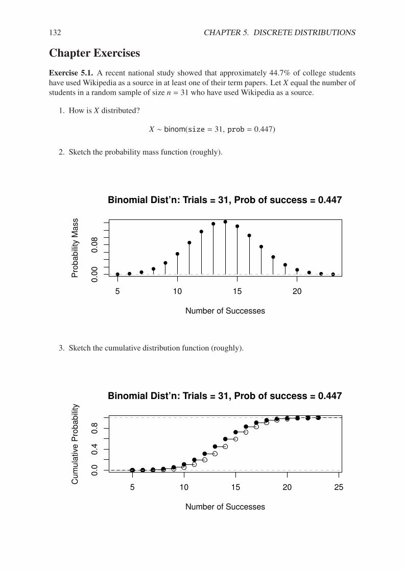
132 CHAPTER 5. DISCRETE DISTRIBUTIONS
Chapter Exercises
Exercise 5.1. A recent national study showed that approximately 44.7% of college studentshave used Wikipedia as a source in at least one of their term papers. Let X equal the number ofstudents in a random sample of size n = 31 who have used Wikipedia as a source.
1. How is X distributed?
X 4 binom(size = 31, prob = 0.447)
2. Sketch the probability mass function (roughly).
5 10 15 20
0.0
00.0
8
Binomial Dist’n: Trials = 31, Prob of success = 0.447
Number of Successes
Pro
babili
ty M
ass
3. Sketch the cumulative distribution function (roughly).
5 10 15 20 25
0.0
0.4
0.8
Binomial Dist’n: Trials = 31, Prob of success = 0.447
Number of Successes
Cum
ula
tive P
robabili
ty
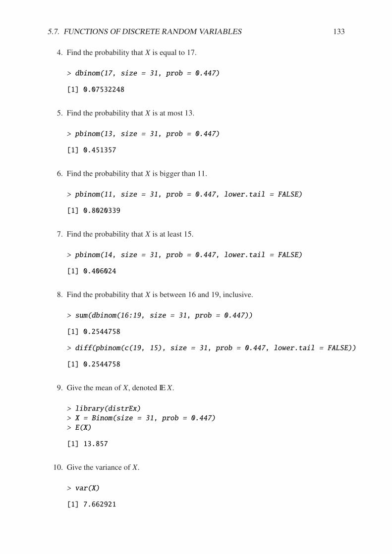
5.7. FUNCTIONS OF DISCRETE RANDOM VARIABLES 133
4. Find the probability that X is equal to 17.
> dbinom(17, size = 31, prob = 0.447)
[1] 0.07532248
5. Find the probability that X is at most 13.
> pbinom(13, size = 31, prob = 0.447)
[1] 0.451357
6. Find the probability that X is bigger than 11.
> pbinom(11, size = 31, prob = 0.447, lower.tail = FALSE)
[1] 0.8020339
7. Find the probability that X is at least 15.
> pbinom(14, size = 31, prob = 0.447, lower.tail = FALSE)
[1] 0.406024
8. Find the probability that X is between 16 and 19, inclusive.
> sum(dbinom(16:19, size = 31, prob = 0.447))
[1] 0.2544758
> diff(pbinom(c(19, 15), size = 31, prob = 0.447, lower.tail = FALSE))
[1] 0.2544758
9. Give the mean of X, denoted IE X.
> library(distrEx)
> X = Binom(size = 31, prob = 0.447)
> E(X)
[1] 13.857
10. Give the variance of X.
> var(X)
[1] 7.662921

134 CHAPTER 5. DISCRETE DISTRIBUTIONS
11. Give the standard deviation of X.
> sd(X)
[1] 2.768198
12. Find IE(4X + 51.324)
> E(4 * X + 51.324)
[1] 106.752
Exercise 5.2. For the following situations, decide what the distribution of X should be. Innearly every case, there are additional assumptions that should be made for the distribution toapply; identify those assumptions (which may or may not hold in practice.)
1. We shoot basketballs at a basketball hoop, and count the number of shots until we makea goal. Let X denote the number of missed shots. On a normal day we would typicallymake about 37% of the shots.
2. In a local lottery in which a three digit number is selected randomly, let X be the numberselected.
3. We drop a Styrofoam cup to the floor twenty times, each time recording whether the cupcomes to rest perfectly right side up, or not. Let X be the number of times the cup landsperfectly right side up.
4. We toss a piece of trash at the garbage can from across the room. If we miss the trashcan, we retrieve the trash and try again, continuing to toss until we make the shot. Let Xdenote the number of missed shots.
5. Working for the border patrol, we inspect shipping cargo as when it enters the harborlooking for contraband. A certain ship comes to port with 557 cargo containers. Stan-dard practice is to select 10 containers randomly and inspect each one very carefully,classifying it as either having contraband or not. Let X count the number of containersthat illegally contain contraband.
6. At the same time every year, some migratory birds land in a bush outside for a short rest.On a certain day, we look outside and let X denote the number of birds in the bush.
7. We count the number of rain drops that fall in a circular area on a sidewalk during a tenminute period of a thunder storm.
8. We count the number of moth eggs on our window screen.
9. We count the number of blades of grass in a one square foot patch of land.
10. We count the number of pats on a baby’s back until (s)he burps.
Exercise 5.3. Find the constant c so that the given function is a valid PDF of a random variableX.
5.7. FUNCTIONS OF DISCRETE RANDOM VARIABLES 135
1. f (x) = Cxn, 0 < x < 1.
2. f (x) = Cxe#x, 0 < x < &.
3. f (x) = e#(x#C), 7 < x < &.
4. f (x) = Cx3(1 # x)2, 0 < x < 1.
5. f (x) = C(1 + x2/4)#1, #& < x < &.
Exercise 5.4. Show that IE(X # µ)2 = IE X2 # µ2. Hint: expand the quantity (X # µ)2 anddistribute the expectation over the resulting terms.
Exercise 5.5. If X 4 binom(size = n, prob = p) show that IE X(X # 1) = n(n # 1)p2.
Exercise 5.6. Calculate the mean and variance of the hypergeometric distribution. Show that
µ = KM
M + N, "2 = K
MN
(M + N)2M + N # K
M + N # 1. (5.7.4)

136 CHAPTER 5. DISCRETE DISTRIBUTIONS

Chapter 6
Continuous Distributions
The focus of the last chapter was on random variables whose support can be written down ina list of values (finite or countably infinite), such as the number of successes in a sequence ofBernoulli trials. Now we move to random variables whose support is a whole range of values,say, an interval (a, b). It is shown in later classes that it is impossible to write all of the numbersdown in a list; there are simply too many of them.
This chapter begins with continuous random variables and the associated PDFs and CDFsThe continuous uniform distribution is highlighted, along with the Gaussian, or normal, distri-bution. Some mathematical details pave the way for a catalogue of models.
The interested reader who would like to learn more about any of the assorted discrete distri-butions mentioned below should take a look at Continuous Univariate Distributions, Volumes1 and 2 by Johnson et al [47, 48].
What do I want them to know?
• how to choose a reasonable continuous model under a variety of physical circumstances
• basic correspondence between continuous versus discrete random variables
• the general tools of the trade for manipulation of continuous random variables, integra-tion, etc.
• some details on a couple of continuous models, and exposure to a bunch of other ones
• how to make new continuous random variables from old ones
6.1 Continuous Random Variables
6.1.1 Probability Density Functions
Continuous random variables have supports that look like
S X = [a, b] or (a, b), (6.1.1)
or unions of intervals of the above form. Examples of random variables that are often taken tobe continuous are:
• the height or weight of an individual,
137
138 CHAPTER 6. CONTINUOUS DISTRIBUTIONS
• other physical measurements such as the length or size of an object, and
• durations of time (usually).
Every continuous random variable X has a probability density function (PDF) denoted fX asso-ciated with it1 that satisfies three basic properties:
1. fX(x) > 0 for x 3 S X,
2.Ax3S X
fX(x) dx = 1, and
3. IP(X 3 A) =Ax3A
fX(x) dx, for an event A 0 S X.
Remark 6.1. We can say the following about continuous random variables:
• Usually, the set A in 3 takes the form of an interval, for example, A = [c, d], in whichcase
IP(X 3 A) =
B d
c
fX(x) dx. (6.1.2)
• It follows that the probability that X falls in a given interval is simply the area under the
curve of fX over the interval.
• Since the area of a line x = c in the plane is zero, IP(X = c) = 0 for any value c. Inother words, the chance that X equals a particular value c is zero, and this is true for anynumber c. Moreover, when a < b all of the following probabilities are the same:
IP(a " X " b) = IP(a < X " b) = IP(a " X < b) = IP(a < X < b). (6.1.3)
• The PDF fX can sometimes be greater than 1. This is in contrast to the discrete case;every nonzero value of a PMF is a probability which is restricted to lie in the interval[0, 1].
We met the cumulative distribution function, FX, in Chapter 5. Recall that it is defined byFX(t) = IP(X " t), for #& < t < &. While in the discrete case the CDF is unwieldy, in thecontinuous case the CDF has a relatively convenient form:
FX(t) = IP(X " t) =
B t
#&fX(x) dx, #& < t < &. (6.1.4)
Remark 6.2. For any continuous CDF FX the following are true.
• FX is nondecreasing , that is, t1 " t2 implies FX(t1) " FX(t2).
• FX is continuous (see Appendix E.2). Note the distinction from the discrete case: CDFsof discrete random variables are not continuous, they are only right continuous.
• limt.#& FX(t) = 0 and limt.& FX(t) = 1.
There is a handy relationship between the CDF and PDF in the continuous case. Considerthe derivative of FX:
F5X(t) =
d
dtFX(t) =
d
dt
B t
#&fX(x) dx = fX(t), (6.1.5)
the last equality being true by the Fundamental Theorem of Calculus, part (2) (see AppendixE.2). In short, (FX)
5 = fX in the continuous case2.
1Not true. There are pathological random variables with no density function. (This is one of the crazy thingsthat can happen in the world of measure theory). But in this book we will not get even close to these anomalousbeasts, and regardless it can be proved that the CDF always exists.
2In the discrete case, fX(x) = FX(x) # limt.x# FX(t).
6.1. CONTINUOUS RANDOM VARIABLES 139
6.1.2 Expectation of Continuous Random Variables
For a continuous random variable X the expected value of g(X) is
IE g(X) =
B
x3Sg(x) fX(x) dx, (6.1.6)
provided the (potentially improper) integralAS|g(x)| f (x)dx is convergent. One important ex-
ample is the mean µ, also known as IE X:
µ = IE X =
B
x3Sx fX(x) dx, (6.1.7)
providedAS|x| f (x)dx is finite. Also there is the variance
"2 = IE(X # µ)2 =B
x3S(x # µ)2 fX(x) dx, (6.1.8)
which can be computed with the alternate formula "2 = IE X2 # (IE X)2. In addition, there isthe standard deviation " =
$"2. The moment generating function is given by
MX(t) = IE etX =
B &
#&etx fX(x) dx, (6.1.9)
provided the integral exists (is finite) for all t in a neighborhood of t = 0.
Example 6.3. Let the continuous random variable X have PDF
fX(x) = 3x2, 0 " x " 1.
We will see later that fX belongs to the Beta family of distributions. It is easy to see thatA &
#&f (x)dx = 1.
B &
#&fX(x)dx =
B 1
0
3x2 dx
= x34441x=0
= 13 # 03
= 1.
This being said, we may find IP(0.14 " X < 0.71).
IP(0.14 " X < 0.71) =
B 0.71
0.14
3x2dx,
= x34440.71x=0.14
= 0.713 # 0.143
' 0.355167.
We can find the mean and variance in an identical manner.
µ =
B &
#&x fX(x)dx =
B 1
0
x · 3x2 dx,
=3
4x4|1x=0,
=3
4.
It would perhaps be best to calculate the variance with the shortcut formula "2 = IE X2 # µ2:
140 CHAPTER 6. CONTINUOUS DISTRIBUTIONS
IE X2 =
B &
#&x2 fX(x)dx =
B 1
0
x2 · 3x2 dx
=3
5x5
444441
x=0
= 3/5.
which gives "2 = 3/5 # (3/4)2 = 3/80.
Example 6.4. We will try one with unbounded support to brush up on improper integration.Let the random variable X have PDF
fX(x) =3
x4, x > 1.
We can show thatA &
#&f (x)dx = 1:
B &
#&fX(x)dx =
B &
1
3
x4dx
= limt.&
B t
1
3
x4dx
= limt.&
31
#3x#3
44444t
x=1
= #0limt.&
1
t3# 1
1
= 1.
We calculate IP(3.4 " X < 7.1):
IP(3.4 " X < 7.1) =
B 7.1
3.4
3x#4dx
= 31
#3x#3
444447.1
x=3.4
= #1(7.1#3 # 3.4#3)
' 0.0226487123.
We locate the mean and variance just like before.
µ =
B &
#&x fX(x)dx =
B &
1
x ·3
x4dx
= 31
#2x#2
44444&
x=1
= #3
2
0limt.&
1
t2# 1
1
=3
2.
6.1. CONTINUOUS RANDOM VARIABLES 141
Again we use the shortcut "2 = IE X2 # µ2:
IE X2 =
B &
#&x2 fX(x)dx =
B &
1
x2 ·3
x4dx
= 31
#1x#1
44444&
x=1
= #30limt.&
1
t2# 1
1
= 3,
which closes the example with "2 = 3 # (3/2)2 = 3/4.
6.1.3 How to do it with R
There exist utilities to calculate probabilities and expectations for general continuous randomvariables, but it is better to find a built-in model, if possible. Sometimes it is not possible. Weshow how to do it the long way, and the distr package way.
Example 6.5. Let X have PDF f (x) = 3x2, 0 < x < 1 and find IP(0.14 " X " 0.71). (We willignore that X is a beta random variable for the sake of argument.)
> f <- function(x) 3 * x^2
> integrate(f, lower = 0.14, upper = 0.71)
0.355167 with absolute error < 3.9e-15
Compare this to the answer we found in Example 6.3. We could integrate the functionx f (x) = 3*x^3 from zero to one to get the mean, and use the shortcut "2 = IE X2 # (IE X)2 forthe variance.
Example 6.6. Let X have PDF f (x) = 3/x4, x > 1. We may integrate the function x f (x) =3/x^3 from zero to infinity to get the mean of X.
> g <- function(x) 3/x^3
> integrate(g, lower = 1, upper = Inf)
1.5 with absolute error < 1.7e-14
Compare this to the answer we got in Example 6.4. Use -Inf for #&.
Example 6.7. Let us redo Example 6.3 with the distr package. The method is similar tothat encountered in Section 5.1.3 in Chapter 5. We define an absolutely continuous randomvariable:
> library(distr)
> f <- function(x) 3 * x^2
> X <- AbscontDistribution(d = f, low1 = 0, up1 = 1)
> p(X)(0.71) - p(X)(0.14)
[1] 0.355167
142 CHAPTER 6. CONTINUOUS DISTRIBUTIONS
Compare this answers we found earlier. Now let us try expectation with the distrExpackage [74]:
> library(distrEx)
> E(X)
[1] 0.7496337
> var(X)
[1] 0.03768305
> 3/80
[1] 0.0375
Compare these answers to the ones we found in Example 6.3. Why are they di!erent?Because the distrEx package resorts to numerical methods when it encounters a model itdoes not recognize. This means that the answers we get for calculations may not exactly matchthe theoretical values. Be careful.
6.2 The Continuous Uniform Distribution
A random variable X with the continuous uniform distribution on the interval (a, b) has PDF
fX(x) =1
b # a, a < x < b. (6.2.1)
The associated R function is dunif(min = a, max = b). We write X 4 unif(min = a, max = b).Due to the particularly simple form of this PDF we can also write down explicitly a formulafor the CDF FX:
FX(t) =
9:::::;:::::<
0, t < 0,t#ab#a , a " t < b,
1, t / b.
(6.2.2)
The continuous uniform distribution is the continuous analogue of the discrete uniform dis-tribution; it is used to model experiments whose outcome is an interval of numbers that are“equally likely” in the sense that any two intervals of equal length in the support have the sameprobability associated with them.
Example 6.8. Choose a number in [0,1] at random, and let X be the number chosen. ThenX 4 unif(min = 0, max = 1).
The mean of X 4 unif(min = a, max = b) is relatively simple to calculate:
µ = IE X =
B &
#&x fX(x) dx,
=
B b
a
x1
b # adx,
=1
b # a
x2
2
444444
b
x=a
,
=1
b # a
b2 # a2
2,
=b + a
2,

6.3. THE NORMAL DISTRIBUTION 143
using the popular formula for the di!erence of squares. The variance is left to Exercise 6.4.
6.3 The Normal Distribution
We say that X has a normal distribution if it has PDF
fX(x) =1
"$2&
exp
.#(x # µ)2
2"2
/, #& < x < &. (6.3.1)
We write X 4 norm(mean = µ, sd = "), and the associated R function is dnorm(x, mean =0, sd = 1).
The familiar bell-shaped curve, the normal distribution is also known as theGaussian distri-bution because the German mathematician C. F. Gauss largely contributed to its mathematicaldevelopment. This distribution is by far the most important distribution, continuous or discrete.The normal model appears in the theory of all sorts of natural phenomena, from to the wayparticles of smoke dissipate in a closed room, to the journey of a bottle in the ocean to thewhite noise of cosmic background radiation.
When µ = 0 and " = 1 we say that the random variable has a standard normal distributionand we typically write Z 4 norm(mean = 0, sd = 1). The lowercase Greek letter phi (') isused to denote the standard normal PDF and the capital Greek letter phi $ is used to denote thestandard normal CDF: for #& < z < &,
'(z) =1
$2&
e#z2/2 and $(t) =
B t
#&'(z) dz. (6.3.2)
Proposition 6.9. If X 4 norm(mean = µ, sd = ") then
Z =X # µ"
4 norm(mean = 0, sd = 1). (6.3.3)
The MGF of Z 4 norm(mean = 0, sd = 1) is relatively easy to derive:
MZ(t) =
B &
#&etz
1$2&
e#z2/2dz,
=
B &
#&
1$2&
exp
.#1
2
2z2 + 2tz + t2
3+t2
2
/dz,
= et2/2
0B &
#&
1$2&
e#[z#(#t)]2/2dz
1,
and the quantity in the parentheses is the total area under a norm(mean = #t, sd = 1) density,which is one. Therefore,
MZ(t) = e#t2/2, #& < t < &. (6.3.4)
Example 6.10. The MGF of X 4 norm(mean = µ, sd = ") is then not di"cult either because
Z =X # µ", or rewriting, X = "Z + µ.
Therefore:MX(t) = IE etX = IE et("Z+µ) = IE e"tXeµ = etµMZ("t),
and we know that MZ(t) = et2/2, thus substituting we get
MX(t) = etµe("t)2/2 = exp
5µt + "2t2/2
6,
for #& < t < &.
144 CHAPTER 6. CONTINUOUS DISTRIBUTIONS
Fact 6.11. The same argument above shows that if X has MGF MX(t) then the MGF of Y =
a + bX is
MY (t) = etaMX(bt). (6.3.5)
Example 6.12. The 68-95-99.7 Rule. We saw in Section 3.3.6 that when an empirical distribu-tion is approximately bell shaped there are specific proportions of the observations which fallat varying distances from the (sample) mean. We can see where these come from – and obtainmore precise proportions – with the following:
> pnorm(1:3) - pnorm(-(1:3))
[1] 0.6826895 0.9544997 0.9973002
Example 6.13. Let the random experiment consist of a person taking an IQ test, and let X bethe score on the test. The scores on such a test are typically standardized to have a mean of 100and a standard deviation of 15. What is IP(85 " X " 115)?
Solution: this one is easy because the limits 85 and 115 fall exactly one standard deviation(below and above, respectively) from the mean of 100. The answer is therefore approximately68%.
6.3.1 Normal Quantiles and the Quantile Function
Until now we have been given two values and our task has been to find the area under the PDFbetween those values. In this section, we go in reverse: we are given an area, and we wouldlike to find the value(s) that correspond to that area.
Example 6.14. Assuming the IQ model of Example 6.13, what is the lowest possible IQ scorethat a person can have and still be in the top 1% of all IQ scores?
Solution: If a person is in the top 1%, then that means that 99% of the people have lowerIQ scores. So, in other words, we are looking for a value x such that F(x) = IP(X " x)satisfies F(x) = 0.99, or yet another way to say it is that we would like to solve the equationF(x)#0.99 = 0. For the sake of argument, let us see how to do this the long way. We define thefunction g(x) = F(x) # 0.99, and then look for the root of g with the uniroot function. It usesnumerical procedures to find the root so we need to give it an interval of x values in which tosearch for the root. We can get an educated guess from the Empirical Rule 3.13; the root shouldbe somewhere between two and three standard deviations (15 each) above the mean (which is100).
> g <- function(x) pnorm(x, mean = 100, sd = 15) - 0.99
> uniroot(g, interval = c(130, 145))
$root
[1] 134.8952
$f.root
[1] -4.873083e-09
$iter
[1] 6
$estim.prec
[1] 6.103516e-05

6.3. THE NORMAL DISTRIBUTION 145
The answer is shown in $root which is approximately 134.8952, that is, a person with thisIQ score or higher falls in the top 1% of all IQ scores.
The discussion in example 6.14 was centered on the search for a value x that solved anequation F(x) = p, for some given probability p, or in mathematical parlance, the search forF#1, the inverse of the CDF of X, evaluated at p. This is so important that it merits a definitionall its own.
Definition 6.15. The quantile function3 of a random variable X is the inverse of its cumulativedistribution function:
QX(p) = min {x : FX(x) / p} , 0 < p < 1. (6.3.6)
Remark 6.16. Here are some properties of quantile functions:
1. The quantile function is defined and finite for all 0 < p < 1.
2. QX is left-continuous (see Appendix E.2). For discrete random variables it is a stepfunction, and for continuous random variables it is a continuous function.
3. In the continuous case the graph of QX may be obtained by reflecting the graph of FX
about the line y = x. In the discrete case, before reflecting one should: 1) connect thedots to get rid of the jumps – this will make the graph look like a set of stairs, 2) erasethe horizontal lines so that only vertical lines remain, and finally 3) swap the open circleswith the solid dots. Please see Figure 5.3.2 for a comparison.
4. The two limitslimp.0+
QX(p) and limp.1#
QX(p)
always exist, but may be infinite (that is, sometimes limp.0 Q(p) = #& and/or limp.1 Q(p) =&).
As the reader might expect, the standard normal distribution is a very special case and hasits own special notation.
Definition 6.17. For 0 < ( < 1, the symbol z( denotes the unique solution of the equationIP(Z > z() = (, where Z 4 norm(mean = 0, sd = 1). It can be calculated in one of twoequivalent ways: qnorm(1 # () and qnorm((, lower.tail = FALSE).
There are a few other very important special cases which we will encounter in later chapters.
6.3.2 How to do it with R
Quantile functions are defined for all of the base distributions with the q prefix to the distribu-tion name, except for the ECDF whose quantile function is exactly the Qx(p) =quantile(x,probs = p , type = 1) function.
Example 6.18. Back to Example 6.14, we are looking for QX(0.99), where X 4 norm(mean =100, sd = 15). It could not be easier to do with R.
> qnorm(0.99, mean = 100, sd = 15)
3The precise definition of the quantile function is QX(p) = inf {x : FX(x) / p}, so at least it is well defined(though perhaps infinite) for the values p = 0 and p = 1.
146 CHAPTER 6. CONTINUOUS DISTRIBUTIONS
[1] 134.8952
Compare this answer to the one obtained earlier with uniroot.
Example 6.19. Find the values z0.025, z0.01, and z0.005 (these will play an important role fromChapter 9 onward).
> qnorm(c(0.025, 0.01, 0.005), lower.tail = FALSE)
[1] 1.959964 2.326348 2.575829
Note the lower.tail argument. We would get the same answer with
qnorm(c(0.975, 0.99, 0.995))
6.4 Functions of Continuous Random Variables
The goal of this section is to determine the distribution of U = g(X) based on the distributionof X. In the discrete case all we needed to do was back substitute for x = g#1(u) in the PMF ofX (sometimes accumulating probability mass along the way). In the continuous case, however,we need more sophisticated tools. Now would be a good time to review Appendix E.2.
6.4.1 The PDF Method
Proposition 6.20. Let X have PDF fX and let g be a function which is one-to-one with a
di"erentiable inverse g#1. Then the PDF of U = g(X) is given by
fU(u) = fXCg#1(u)
D 44444d
dug#1(u)
44444 . (6.4.1)
Remark 6.21. The formula in Equation 6.4.1 is nice, but does not really make any sense. It isbetter to write in the intuitive form
fU(u) = fX(x)
44444dx
du
44444 . (6.4.2)
Example 6.22. Let X 4 norm(mean = µ, sd = "), and let Y = eX. What is the PDF of Y?Solution: Notice first that ex > 0 for any x, so the support of Y is (0,&). Since the transfor-
mation is monotone, we can solve y = ex for x to get x = ln y, giving dx/dy = 1/y. Therefore,for any y > 0,
fY(y) = fX(ln y) ·444441
y
44444 =1
"$2&
exp
.(ln y # µ)2
2"2
/·1
y,
where we have dropped the absolute value bars since y > 0. The random variable Y is said tohave a lognormal distribution; see Section 6.5.
Example 6.23. Suppose X 4 norm(mean = 0, sd = 1) and let Y = 4# 3X. What is the PDF ofY?
6.4. FUNCTIONS OF CONTINUOUS RANDOM VARIABLES 147
The support of X is (#&,&), and as x goes from #& to &, the quantity y = 4 # 3x alsotraverses (#&,&). Solving for x in the equation y = 4 # 3x yields x = #(y # 4)/3 givingdx/dy = #1/3. And since
fX(x) =1
$2&
e#x2/2, #& < x < &,
we have
fY(y) = fX
0y # 4
3
1·
44444#1
3
44444 , #& < y < &,
=1
3$2&
e#(y#4)2/2·32 , #& < y < &.
We recognize the PDF of Y to be that of a norm(mean = 4, sd = 3) distribution. Indeed, wemay use an identical argument as the above to prove the following fact:
Fact 6.24. If X 4 norm(mean = µ, sd = ") and if Y = a + bX for constants a and b, with
b ! 0, then Y 4 norm(mean = a + bµ, sd = |b|").
Note that it is sometimes easier to postpone solving for the inverse transformation x = x(u).Instead, leave the transformation in the form u = u(x) and calculate the derivative of the originaltransformation
du/dx = g5(x). (6.4.3)
Once this is known, we can get the PDF of U with
fU(u) = fX(x)
444441
du/dx
44444 . (6.4.4)
In many cases there are cancellations and the work is shorter. Of course, it is not always truethat
dx
du=
1
du/dx, (6.4.5)
but for the well-behaved examples in this book the trick works just fine.
Remark 6.25. In the case that g is not monotone we cannot apply Proposition 6.20 directly.However, hope is not lost. Rather, we break the support of X into pieces such that g is monotoneon each one. We apply Proposition 6.20 on each piece, and finish up by adding the resultstogether.
6.4.2 The CDF method
We know from Section 6.1 that fX = F5X in the continuous case. Starting from the equation
FY(y) = IP(Y " y), we may substitute g(X) for Y , then solve for X to obtain IP[X " g#1(y)],which is just another way to write FX[g
#1(y)]. Di!erentiating this last quantity with respect toy will yield the PDF of Y .
Example 6.26. Suppose X 4 unif(min = 0, max = 1) and suppose that we let Y = # ln X.What is the PDF of Y?
The support set of X is (0, 1), and y traverses (0,&) as x ranges from 0 to 1, so the supportset of Y is S Y = (0,&). For any y > 0, we consider
FY(y) = IP(Y " y) = IP(# ln X " y) = IP(X / e#y) = 1 # IP(X < e#y),
148 CHAPTER 6. CONTINUOUS DISTRIBUTIONS
where the next to last equality follows because the exponential function is monotone (this pointwill be revisited later). Now since X is continuous the two probabilities IP(X < e#y) andIP(X " e#y) are equal; thus
1 # IP(X < e#y) = 1 # IP(X " e#y) = 1 # FX(e#y).
Now recalling that the CDF of a unif(min = 0, max = 1) random variable satisfies F(u) = u
(see Equation 6.2.2), we can say
FY(y) = 1 # FX(e#y) = 1 # e#y, for y > 0.
We have consequently found the formula for the CDF of Y; to obtain the PDF fY we need onlydi!erentiate FY :
fY(y) =d
dy
=1 # e#y
>= 0 # e#y(#1),
or fY(y) = e#y for y > 0. This turns out to be a member of the exponential family of distribu-tions, see Section 6.5.
Example 6.27. The Probability Integral Transform. Given a continuous random variable X
with strictly increasing CDF FX, let the random variable Y be defined by Y = FX(X). Then thedistribution of Y is unif(min = 0, max = 1).
Proof. We employ the CDF method. First note that the support of Y is (0, 1). Then for any0 < y < 1,
FY(y) = IP(Y " y) = IP(FX(X) " y).
Now since FX is strictly increasing, it has a well defined inverse function F#1X . Therefore,
IP(FX(X) " y) = IP(X " F#1X (y)) = FX[F
#1X (y)] = y.
Summarizing, we have seen that FY(y) = y, 0 < y < 1. But this is exactly the CDF of aunif(min = 0, max = 1) random variable. "
Fact 6.28. The Probability Integral Transform is true for all continuous random variables with
continuous CDFs, not just for those with strictly increasing CDFs (but the proof is more com-
plicated). The transform is not true for discrete random variables, or for continuous random
variables having a discrete component (that is, with jumps in their CDF).
Example 6.29. Let Z 4 norm(mean = 0, sd = 1) and let U = Z2. What is the PDF of U?Notice first that Z2 / 0, and thus the support of U is [0,&). And for any u / 0,
FU(u) = IP(U " u) = IP(Z2 " u).
But Z2 " u occurs if and only if #$u " Z "
$u. The last probability above is simply the area
under the standard normal PDF from #$u to
$u, and since ' is symmetric about 0, we have
IP(Z2 " u) = 2 IP(0 " Z "$u) = 2
CFZ(
$u) # FZ(0)
D= 2$(
$u) # 1,
because $(0) = 1/2. To find the PDF of U we di!erentiate the CDF recalling that $5 = '.
fU(u) =22$(
$u) # 1
35= 2'(
$u) ·
1
2$u= u#1/2'(
$u).
Substituting,
fU(u) = u#1/21
$2&
e#($u)2/2 = (2&u)#1/2e#u, u > 0.
This is what we will later call a chi-square distribution with 1 degree of freedom. See Section6.5.
6.4. FUNCTIONS OF CONTINUOUS RANDOM VARIABLES 149
6.4.3 How to do it with R
The distr package has functionality to investigate transformations of univariate distributions.There are exact results for ordinary transformations of the standard distributions, and distrtakes advantage of these in many cases. For instance, the distr package can handle the trans-formation in Example 6.23 quite nicely:
> library(distr)
> X <- Norm(mean = 0, sd = 1)
> Y <- 4 - 3 * X
> Y
Distribution Object of Class: Norm
mean: 4
sd: 3
So distr “knows” that a linear transformation of a normal random variable is again normal,and it even knows what the correct mean and sd should be. But it is impossible for distr toknow everything, and it is not long before we venture outside of the transformations that distrrecognizes. Let us try Example 6.22:
> Y <- exp(X)
> Y
Distribution Object of Class: AbscontDistribution
The result is an object of class AbscontDistribution, which is one of the classes thatdistr uses to denote general distributions that it does not recognize (it turns out that Z has alognormal distribution; see Section 6.5). A simplified description of the process that distrundergoes when it encounters a transformation Y = g(X) that it does not recognize is
1. Randomly generate many, many copies X1, X2, . . . , Xn from the distribution of X,
2. Compute Y1 = g(X1), Y2 = g(X2), . . . , Yn = g(Xn) and store them for use.
3. Calculate the PDF, CDF, quantiles, and random variates using the simulated values of Y .
As long as the transformation is su"ciently nice, such as a linear transformation, the expo-nential, absolute value, etc., the d-p-q functions are calculated analytically based on the d-p-qfunctions associated with X. But if we try a crazy transformation then we are greeted by awarning:
> W <- sin(exp(X) + 27)
> W
Distribution Object of Class: AbscontDistribution
The warning confirms that the d-p-q functions are not calculated analytically, but are insteadbased on the randomly simulated values of Y . We must be careful to remember this. The natureof random simulationmeans that we can get di!erent answers to the same question: watch whathappens when we compute IP(W " 0.5) using theW above, then define W again, and computethe (supposedly) same IP(W " 0.5) a few moments later.

150 CHAPTER 6. CONTINUOUS DISTRIBUTIONS
> p(W)(0.5)
[1] 0.57988
> W <- sin(exp(X) + 27)
> p(W)(0.5)
[1] 0.5804
The answers are not the same! Furthermore, if we were to repeat the process we would getyet another answer for IP(W " 0.5).
The answers were close, though. And the underlying randomly generated X’s were not thesame so it should hardly be a surprise that the calculated W’s were not the same, either. Thisserves as a warning (in concert with the one that distr provides) that we should be carefulto remember that complicated transformations computed by R are only approximate and mayfluctuate slightly due to the nature of the way the estimates are calculated.
6.5 Other Continuous Distributions
6.5.1 Waiting Time Distributions
In some experiments, the random variable being measured is the time until a certain eventoccurs. For example, a quality control specialist may be testing a manufactured product to seehow long it takes until it fails. An e"ciency expert may be recording the customer tra"c at aretail store to streamline scheduling of sta!.
The Exponential Distribution
We say that X has an exponential distribution and write X 4 exp(rate = %).
fX(x) = %e#%x, x > 0 (6.5.1)
The associated R functions are dexp(x, rate = 1), pexp, qexp, and rexp, which give thePDF, CDF, quantile function, and simulate random variates, respectively.
The parameter % measures the rate of arrivals (to be described later) and must be positive.The CDF is given by the formula
FX(t) = 1 # e#%t, t > 0. (6.5.2)
The mean is µ = 1/% and the variance is "2 = 1/%2.The exponential distribution is closely related to the Poisson distribution. If customers
arrive at a store according to a Poisson process with rate % and if Y counts the number of cus-tomers that arrive in the time interval [0, t), then we saw in Section 5.6 that Y 4 pois(lambda =%t). Now consider a di!erent question: let us start our clock at time 0 and stop the clockwhen the first customer arrives. Let X be the length of this random time interval. ThenX 4 exp(rate = %). Observe the following string of equalities:
IP(X > t) = IP(first arrival after time t),
= IP(no events in [0,t)),
= IP(Y = 0),
= e#%t,
6.5. OTHER CONTINUOUS DISTRIBUTIONS 151
where the last line is the PMF of Y evaluated at y = 0. In other words, IP(X " t) = 1 # e#%t,which is exactly the CDF of an exp(rate = %) distribution.
The exponential distribution is said to bememoryless because exponential random variables"forget" how old they are at every instant. That is, the probability that we must wait an addi-tional five hours for a customer to arrive, given that we have already waited seven hours, isexactly the probability that we needed to wait five hours for a customer in the first place. Inmathematical symbols, for any s, t > 0,
IP(X > s + t | X > t) = IP(X > s). (6.5.3)
See Exercise 6.5.
The Gamma Distribution
This is a generalization of the exponential distribution. We say that X has a gamma distributionand write X 4 gamma(shape = (, rate = %). It has PDF
fX(x) =%(
%(()x(#1e#%x, x > 0. (6.5.4)
The associatedR functions are dgamma(x, shape, rate = 1), pgamma, qgamma, and rgamma,which give the PDF, CDF, quantile function, and simulate random variates, respectively. If( = 1 then X 4 exp(rate = %). The mean is µ = (/% and the variance is "2 = (/%2.
To motivate the gamma distribution recall that if X measures the length of time until thefirst event occurs in a Poisson process with rate % then X 4 exp(rate = %). If we let Y measurethe length of time until the (th event occurs then Y 4 gamma(shape = (, rate = %). When (is an integer this distribution is also known as the Erlang distribution.
Example 6.30. At a car wash, two customers arrive per hour on the average. We decide tomeasure how long it takes until the third customer arrives. If Y denotes this random time thenY 4 gamma(shape = 3, rate = 1/2).
6.5.2 The Chi square, Student’s t, and Snedecor’s F Distributions
The Chi square Distribution
A random variable X with PDF
fX(x) =1
%(p/2)2p/2xp/2#1e#x/2, x > 0, (6.5.5)
is said to have a chi-square distribution with p degrees of freedom. We write X 4 chisq(df =p). The associated R functions are dchisq(x, df), pchisq, qchisq, and rchisq, whichgive the PDF, CDF, quantile function, and simulate random variates, respectively. See Figure6.5.1. In an obvious notation we may define )2((p) as the number on the x-axis such that thereis exactly ( area under the chisq(df = p) curve to its right.
The code to produce Figure 6.5.1 is
> curve(dchisq(x, df = 3), from = 0, to = 20, ylab = "y")
> ind <- c(4, 5, 10, 15)
> for (i in ind) curve(dchisq(x, df = i), 0, 20, add = TRUE)
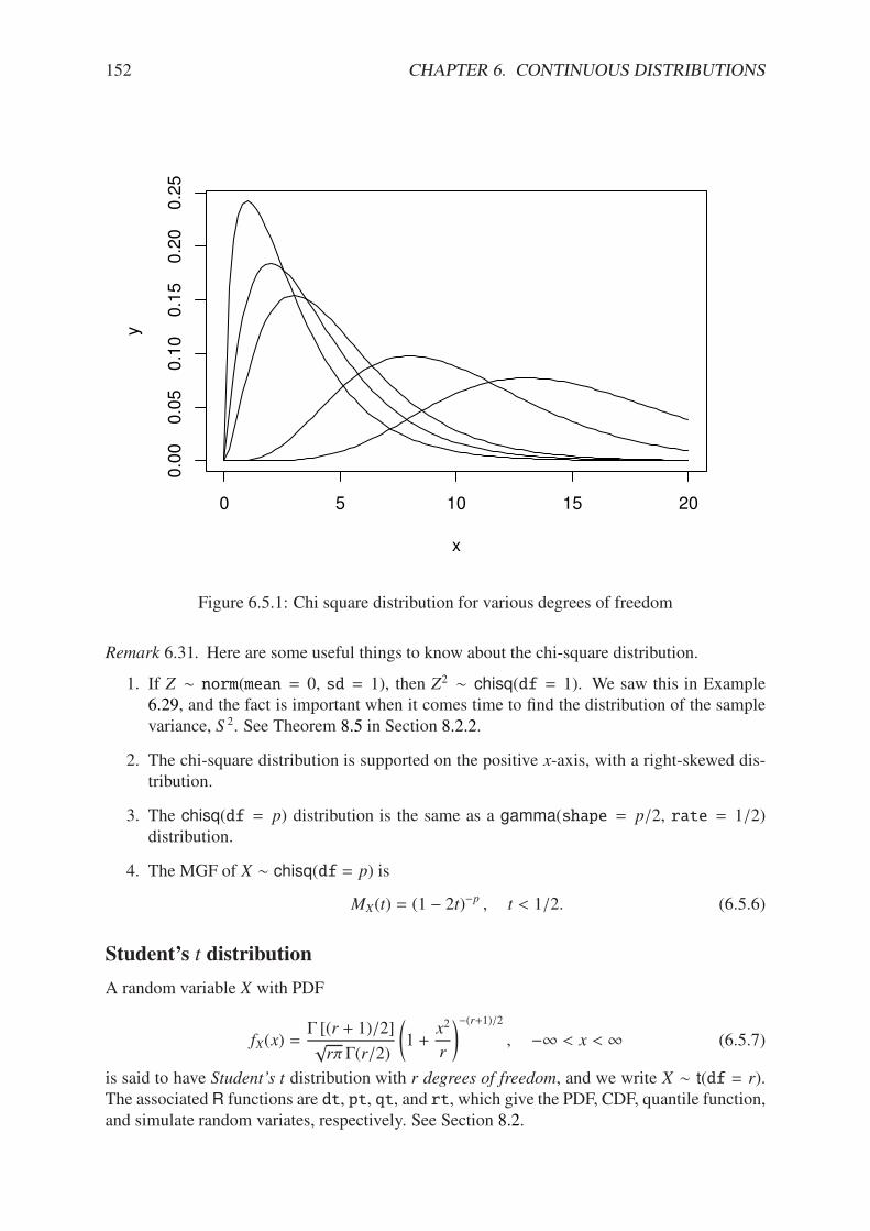
152 CHAPTER 6. CONTINUOUS DISTRIBUTIONS
0 5 10 15 20
0.0
00.0
50.1
00.1
50.2
00.2
5
x
y
Figure 6.5.1: Chi square distribution for various degrees of freedom
Remark 6.31. Here are some useful things to know about the chi-square distribution.
1. If Z 4 norm(mean = 0, sd = 1), then Z2 4 chisq(df = 1). We saw this in Example6.29, and the fact is important when it comes time to find the distribution of the samplevariance, S 2. See Theorem 8.5 in Section 8.2.2.
2. The chi-square distribution is supported on the positive x-axis, with a right-skewed dis-tribution.
3. The chisq(df = p) distribution is the same as a gamma(shape = p/2, rate = 1/2)distribution.
4. The MGF of X 4 chisq(df = p) is
MX(t) = (1 # 2t)#p , t < 1/2. (6.5.6)
Student’s t distribution
A random variable X with PDF
fX(x) =% [(r + 1)/2]$r& %(r/2)
01 +
x2
r
1#(r+1)/2, #& < x < & (6.5.7)
is said to have Student’s t distribution with r degrees of freedom, and we write X 4 t(df = r).The associated R functions are dt, pt, qt, and rt, which give the PDF, CDF, quantile function,and simulate random variates, respectively. See Section 8.2.
6.5. OTHER CONTINUOUS DISTRIBUTIONS 153
Snedecor’s F distribution
A random variable X with p.d.f.
fX(x) =%[(m + n)/2]
%(m/2)%(n/2)
?m
n
@m/2xm/2#1
?1 +
m
nx@#(m+n)/2
, x > 0. (6.5.8)
is said to have an F distribution with (m, n) degrees of freedom. We write X 4 f(df1 =m, df2 = n). The associated R functions are df(x, df1, df2), pf, qf, and rf, whichgive the PDF, CDF, quantile function, and simulate random variates, respectively. We de-fine F((m, n) as the number on the x-axis such that there is exactly ( area under the f(df1 =m, df2 = n) curve to its right.
Remark 6.32. Here are some notes about the F distribution.
1. If X 4 f(df1 = m, df2 = n) and Y = 1/X, then Y 4 f(df1 = n, df2 = m). Historically,this fact was especially convenient. In the old days, statisticians used printed tables fortheir statistical calculations. Since the F tables were symmetric in m and n, it meant thatpublishers could cut the size of their printed tables in half. It plays less of a role todaynow that personal computers are widespread.
2. If X 4 t(df = r), then X2 4 f(df1 = 1, df2 = r). We will see this again in Section 11.3.3.
6.5.3 Other Popular Distributions
The Cauchy Distribution
This is a special case of the Student’s t distribution. It has PDF
fX(x) =1
*&
EFFFFG1 +
0x # m
*
12HIIIIJ#1
, #& < x < & (6.5.9)
We write X 4 cauchy(location = m, scale = *). The associatedR function is dcauchy(x,location = 0, scale = 1).
It is easy to see that a cauchy(location = 0, scale = 1) distribution is the same as at(df = 1) distribution. The cauchy distribution looks like a norm distribution but with veryheavy tails. The mean (and variance) do not exist, that is, they are infinite. The median isrepresented by the location parameter, and the scale parameter influences the spread of thedistribution about its median.
The Beta Distribution
This is a generalization of the continuous uniform distribution.
fX(x) =%(( + *)
%(()%(*)x(#1(1 # x)*#1, 0 < x < 1 (6.5.10)
We write X 4 beta(shape1 = (, shape2 = *). The associated R function is dbeta(x,shape1, shape2). The mean and variance are
µ =(
( + *and "2 =
(*
(( + *)2 (( + * + 1). (6.5.11)
See Example 6.3. This distribution comes up a lot in Bayesian statistics because it is a goodmodel for one’s prior beliefs about a population proportion p, 0 " p " 1.
154 CHAPTER 6. CONTINUOUS DISTRIBUTIONS
The Logistic Distribution
fX(x) =1
"exp
?#x # µ"
@ K1 + exp
?#x # µ"
@L#2, #& < x < &. (6.5.12)
We write X 4 logis(location = µ, scale = "). The associated R function is dlogis(x,location = 0, scale = 1). The logistic distribution comes up in di!erential equations asa model for population growth under certain assumptions. The mean is µ and the variance is&2"2/3.
The Lognormal Distribution
This is a distribution derived from the normal distribution (hence the name). IfU 4 norm(mean =µ, sd = "), then X = eUhas PDF
fX(x) =1
"x$2&
exp
7#(ln x # µ)2
2"2
8, 0 < x < &. (6.5.13)
We write X 4 lnorm(meanlog = µ, sdlog = "). The associated R function is dlnorm(x,meanlog = 0, sdlog = 1). Notice that the support is concentrated on the positive x axis;the distribution is right-skewed with a heavy tail. See Example 6.22.
The Weibull Distribution
This has PDF
fX(x) =(
*
0x
*
1(#1exp
0x
*
1(, x > 0. (6.5.14)
We write X 4 weibull(shape = (, scale = *). The associated R function is dweibull(x,shape, scale = 1).
6.5.4 How to do it with R
There is some support of moments and moment generating functions for some continuous prob-ability distributions included in the actuar package [25]. The convention is m in front of thedistribution name for raw moments, and mgf in front of the distribution name for the momentgenerating function. At the time of this writing, the following distributions are supported:gamma, inverse Gaussian, (non-central) chi-squared, exponential, and uniform.
Example 6.33. Calculate the first four raw moments for X 4 gamma(shape = 13, rate = 1)and plot the moment generating function.
We load the actuar package and use the functions mgamma and mgfgamma:
> library(actuar)
> mgamma(1:4, shape = 13, rate = 1)
[1] 13 182 2730 43680
For the plot we can use the function in the following form:
> plot(function(x) {
+ mgfgamma(x, shape = 13, rate = 1)
+ }, from = -0.1, to = 0.1, ylab = "gamma mgf")
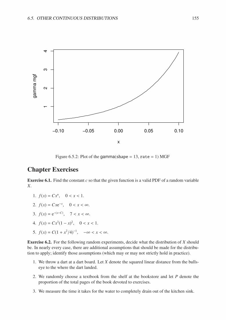
6.5. OTHER CONTINUOUS DISTRIBUTIONS 155
!0.10 !0.05 0.00 0.05 0.10
12
34
x
gam
ma m
gf
Figure 6.5.2: Plot of the gamma(shape = 13, rate = 1) MGF
Chapter Exercises
Exercise 6.1. Find the constant c so that the given function is a valid PDF of a random variableX.
1. f (x) = Cxn, 0 < x < 1.
2. f (x) = Cxe#x, 0 < x < &.
3. f (x) = e#(x#C), 7 < x < &.
4. f (x) = Cx3(1 # x)2, 0 < x < 1.
5. f (x) = C(1 + x2/4)#1, #& < x < &.
Exercise 6.2. For the following random experiments, decide what the distribution of X shouldbe. In nearly every case, there are additional assumptions that should be made for the distribu-tion to apply; identify those assumptions (which may or may not strictly hold in practice).
1. We throw a dart at a dart board. Let X denote the squared linear distance from the bulls-eye to the where the dart landed.
2. We randomly choose a textbook from the shelf at the bookstore and let P denote theproportion of the total pages of the book devoted to exercises.
3. We measure the time it takes for the water to completely drain out of the kitchen sink.
156 CHAPTER 6. CONTINUOUS DISTRIBUTIONS
4. We randomly sample strangers at the grocery store and ask them how long it will takethem to drive home.
Exercise 6.3. If Z is norm(mean = 0, sd = 1), find
1. IP(Z > 2.64)
> pnorm(2.64, lower.tail = FALSE)
[1] 0.004145301
2. IP(0 " Z < 0.87)
> pnorm(0.87) - 1/2
[1] 0.3078498
3. IP(|Z| > 1.39) (Hint: draw a picture!)
> 2 * pnorm(-1.39)
[1] 0.1645289
Exercise 6.4. Calculate the variance of X 4 unif(min = a, max = b). Hint: First calculateIE X2.
type the exercise here
Exercise 6.5. Prove the memoryless property for exponential random variables. That is, forX 4 exp(rate = %) show that for any s, t > 0,
IP(X > s + t | X > t) = IP(X > s).
Chapter 7
Multivariate Distributions
We have built up quite a catalogue of distributions, discrete and continuous. They were allunivariate, however, meaning that we only considered one random variable at a time. We canimagine nevertheless many random variables associated with a single person: their height, theirweight, their wrist circumference (all continuous), or their eye/hair color, shoe size, whetherthey are right handed, left handed, or ambidextrous (all categorical), and we can even surmisereasonable probability distributions to associate with each of these variables.
But there is a di!erence: for a single person, these variables are related. For instance, aperson’s height betrays a lot of information about that person’s weight.
The concept we are hinting at is the notion of dependence between random variables. It isthe focus of this chapter to study this concept in some detail. Along the way, we will pick up ad-ditional models to add to our catalogue. Moreover, we will study certain classes of dependence,and clarify the special case when there is no dependence, namely, independence.
The interested reader who would like to learn more about any of the below mentionedmultivariate distributions should take a look at Discrete Multivariate Distributions by Johnsonet al [49] or Continuous Multivariate Distributions [54] by Kotz et al.
What do I want them to know?
• the basic notion of dependence and how it is manifested with multiple variables (two, inparticular)
• joint versus marginal distributions/expectation (discrete and continuous)
• some numeric measures of dependence
• conditional distributions, in the context of independence and exchangeability
• some details of at least one multivariate model (discrete and continuous)
• what it looks like when there are more than two random variables present
7.1 Joint and Marginal Probability Distributions
Consider two discrete random variables X and Y with PMFs fX and fY that are supported on thesample spaces S X and S Y , respectively. Let S X,Y denote the set of all possible observed pairs
157
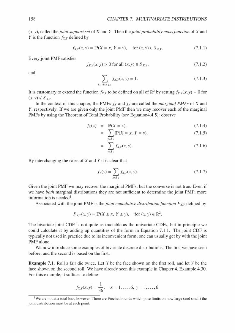
158 CHAPTER 7. MULTIVARIATE DISTRIBUTIONS
(x, y), called the joint support set of X and Y . Then the joint probability mass function of X andY is the function fX,Y defined by
fX,Y(x, y) = IP(X = x, Y = y), for (x, y) 3 S X,Y . (7.1.1)
Every joint PMF satisfiesfX,Y(x, y) > 0 for all (x, y) 3 S X,Y , (7.1.2)
and !
(x,y)3S X,Y
fX,Y(x, y) = 1. (7.1.3)
It is customary to extend the function fX,Y to be defined on all of R2 by setting fX,Y(x, y) = 0 for
(x, y) " S X,Y .In the context of this chapter, the PMFs fX and fY are called the marginal PMFs of X and
Y , respectively. If we are given only the joint PMF then we may recover each of the marginalPMFs by using the Theorem of Total Probability (see Equation4.4.5): observe
fX(x) = IP(X = x), (7.1.4)
=!
y3S Y
IP(X = x, Y = y), (7.1.5)
=!
y3S Y
fX,Y(x, y). (7.1.6)
By interchanging the roles of X and Y it is clear that
fY(y) =!
x3S Y
fX,Y(x, y). (7.1.7)
Given the joint PMF we may recover the marginal PMFs, but the converse is not true. Even ifwe have both marginal distributions they are not su"cient to determine the joint PMF; moreinformation is needed1.
Associated with the joint PMF is the joint cumulative distribution function FX,Y defined by
FX,Y(x, y) = IP(X " x, Y " y), for (x, y) 3 R2.
The bivariate joint CDF is not quite as tractable as the univariate CDFs, but in principle wecould calculate it by adding up quantities of the form in Equation 7.1.1. The joint CDF istypically not used in practice due to its inconvenient form; one can usually get by with the jointPMF alone.
We now introduce some examples of bivariate discrete distributions. The first we have seenbefore, and the second is based on the first.
Example 7.1. Roll a fair die twice. Let X be the face shown on the first roll, and let Y be theface shown on the second roll. We have already seen this example in Chapter 4, Example 4.30.For this example, it su"ces to define
fX,Y(x, y) =1
36, x = 1, . . . , 6, y = 1, . . . , 6.
1We are not at a total loss, however. There are Frechet bounds which pose limits on how large (and small) thejoint distribution must be at each point.
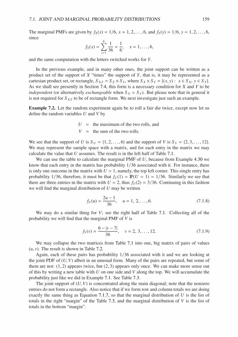
7.1. JOINT AND MARGINAL PROBABILITY DISTRIBUTIONS 159
The marginal PMFs are given by fX(x) = 1/6, x = 1, 2, . . . , 6, and fY(y) = 1/6, y = 1, 2, . . . , 6,since
fX(x) =6!
y=1
1
36=
1
6, x = 1, . . . , 6,
and the same computation with the letters switched works for Y .
In the previous example, and in many other ones, the joint support can be written as aproduct set of the support of X “times” the support of Y , that is, it may be represented as acartesian product set, or rectangle, S X,Y = S X 7 S Y , where S X 7 S Y = {(x, y) : x 3 S X, y 3 S Y}.As we shall see presently in Section 7.4, this form is a necessary condition for X and Y to beindependent (or alternatively exchangeable when S X = S Y). But please note that in general itis not required for S X,Y to be of rectangle form. We next investigate just such an example.
Example 7.2. Let the random experiment again be to roll a fair die twice, except now let usdefine the random variables U and V by
U = the maximum of the two rolls, and
V = the sum of the two rolls.
We see that the support of U is S U = {1, 2, . . . , 6} and the support of V is S V = {2, 3, . . . , 12}.We may represent the sample space with a matrix, and for each entry in the matrix we maycalculate the value that U assumes. The result is in the left half of Table 7.1.
We can use the table to calculate the marginal PMF of U, because from Example 4.30 weknow that each entry in the matrix has probability 1/36 associated with it. For instance, thereis only one outcome in the matrix with U = 1, namely, the top left corner. This single entry hasprobability 1/36, therefore, it must be that fU(1) = IP(U = 1) = 1/36. Similarly we see thatthere are three entries in the matrix with U = 2, thus fU(2) = 3/36. Continuing in this fashionwe will find the marginal distribution of U may be written
fU(u) =2u # 1
36, u = 1, 2, . . . , 6. (7.1.8)
We may do a similar thing for V; see the right half of Table 7.1. Collecting all of theprobability we will find that the marginal PMF of V is
fV(v) =6 # |v # 7|
36, v = 2, 3, . . . , 12. (7.1.9)
We may collapse the two matrices from Table 7.1 into one, big matrix of pairs of values(u, v). The result is shown in Table 7.2.
Again, each of these pairs has probability 1/36 associated with it and we are looking atthe joint PDF of (U,V) albeit in an unusual form. Many of the pairs are repeated, but some ofthem are not: (1, 2) appears twice, but (2, 3) appears only once. We can make more sense outof this by writing a new table with U on one side and V along the top. We will accumulate theprobability just like we did in Example 7.1. See Table 7.3.
The joint support of (U,V) is concentrated along the main diagonal; note that the nonzeroentries do not form a rectangle. Also notice that if we form row and column totals we are doingexactly the same thing as Equation 7.1.7, so that the marginal distribution of U is the list oftotals in the right “margin” of the Table 7.3, and the marginal distribution of V is the list oftotals in the bottom “margin”.
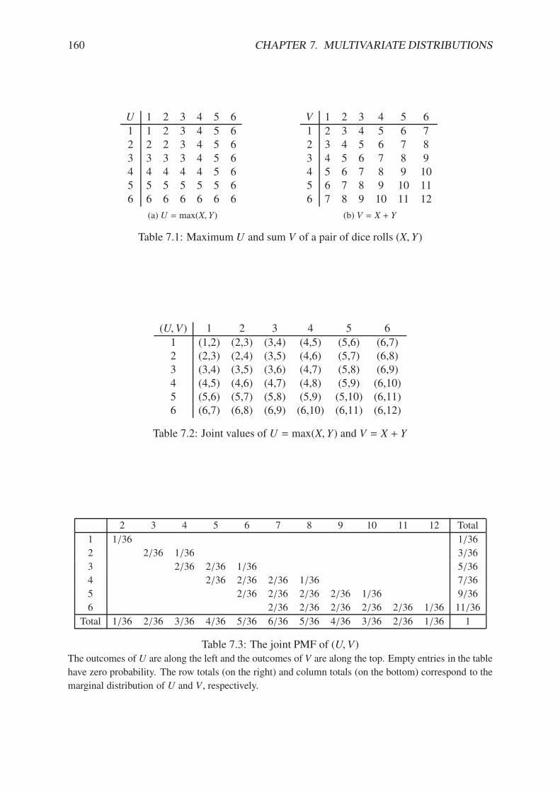
160 CHAPTER 7. MULTIVARIATE DISTRIBUTIONS
U 1 2 3 4 5 61 1 2 3 4 5 62 2 2 3 4 5 63 3 3 3 4 5 64 4 4 4 4 5 65 5 5 5 5 5 66 6 6 6 6 6 6
(a) U = max(X, Y)
V 1 2 3 4 5 61 2 3 4 5 6 72 3 4 5 6 7 83 4 5 6 7 8 94 5 6 7 8 9 105 6 7 8 9 10 116 7 8 9 10 11 12
(b) V = X + Y
Table 7.1: Maximum U and sum V of a pair of dice rolls (X, Y)
(U,V) 1 2 3 4 5 61 (1,2) (2,3) (3,4) (4,5) (5,6) (6,7)2 (2,3) (2,4) (3,5) (4,6) (5,7) (6,8)3 (3,4) (3,5) (3,6) (4,7) (5,8) (6,9)4 (4,5) (4,6) (4,7) (4,8) (5,9) (6,10)5 (5,6) (5,7) (5,8) (5,9) (5,10) (6,11)6 (6,7) (6,8) (6,9) (6,10) (6,11) (6,12)
Table 7.2: Joint values of U = max(X, Y) and V = X + Y
2 3 4 5 6 7 8 9 10 11 12 Total
1 1/36 1/36
2 2/36 1/36 3/36
3 2/36 2/36 1/36 5/36
4 2/36 2/36 2/36 1/36 7/36
5 2/36 2/36 2/36 2/36 1/36 9/36
6 2/36 2/36 2/36 2/36 2/36 1/36 11/36
Total 1/36 2/36 3/36 4/36 5/36 6/36 5/36 4/36 3/36 2/36 1/36 1
Table 7.3: The joint PMF of (U,V)The outcomes of U are along the left and the outcomes of V are along the top. Empty entries in the table
have zero probability. The row totals (on the right) and column totals (on the bottom) correspond to the
marginal distribution of U and V , respectively.
7.1. JOINT AND MARGINAL PROBABILITY DISTRIBUTIONS 161
Continuing the reasoning for the discrete case, given two continuous random variables Xand Y there similarly exists2 a function fX,Y(x, y) associated with X and Y called the joint prob-ability density function of X and Y . Every joint PDF satisfies
fX,Y(x, y) / 0 for all (x, y) 3 S X,Y , (7.1.10)
and "S X,Y
fX,Y(x, y) dx dy = 1. (7.1.11)
In the continuous case there is not such a simple interpretation for the joint PDF; however,we do have one for the joint CDF, namely,
FX,Y(x, y) = IP(X " x, Y " y) =
B x
#&
B y
#&fX,Y(u, v) dv du,
for (x, y) 3 R2. If X and Y have the joint PDF fX,Y , then the marginal density of X may berecovered by
fX(x) =
B
S Y
fX,Y(x, y) dy, x 3 S X (7.1.12)
and the marginal PDF of Y may be found with
fY(y) =
B
S X
fX,Y(x, y) dx, y 3 S Y . (7.1.13)
Example 7.3. Let the joint PDF of (X, Y) be given by
fX,Y(x, y) =6
5
2x + y2
3, 0 < x < 1, 0 < y < 1.
The marginal PDF of X is
fX(x) =
B 1
0
6
5
2x + y2
3dy,
=6
5
0xy +
y3
3
1444444
1
y=0
,
=6
5
0x +
1
3
1,
for 0 < x < 1, and the marginal PDF of Y is
fY(y) =
B 1
0
6
5
2x + y2
3dx,
=6
5
0x2
2+ xy2
1444444
1
x=0
,
=6
5
01
2+ y2
1,
for 0 < y < 1. In this example the joint support set was a rectangle [0, 1] 7 [0, 1], but it turnsout that X and Y are not independent. See Section 7.4.
2Strictly speaking, the joint density function does not necessarily exist. But the joint CDF always exists.
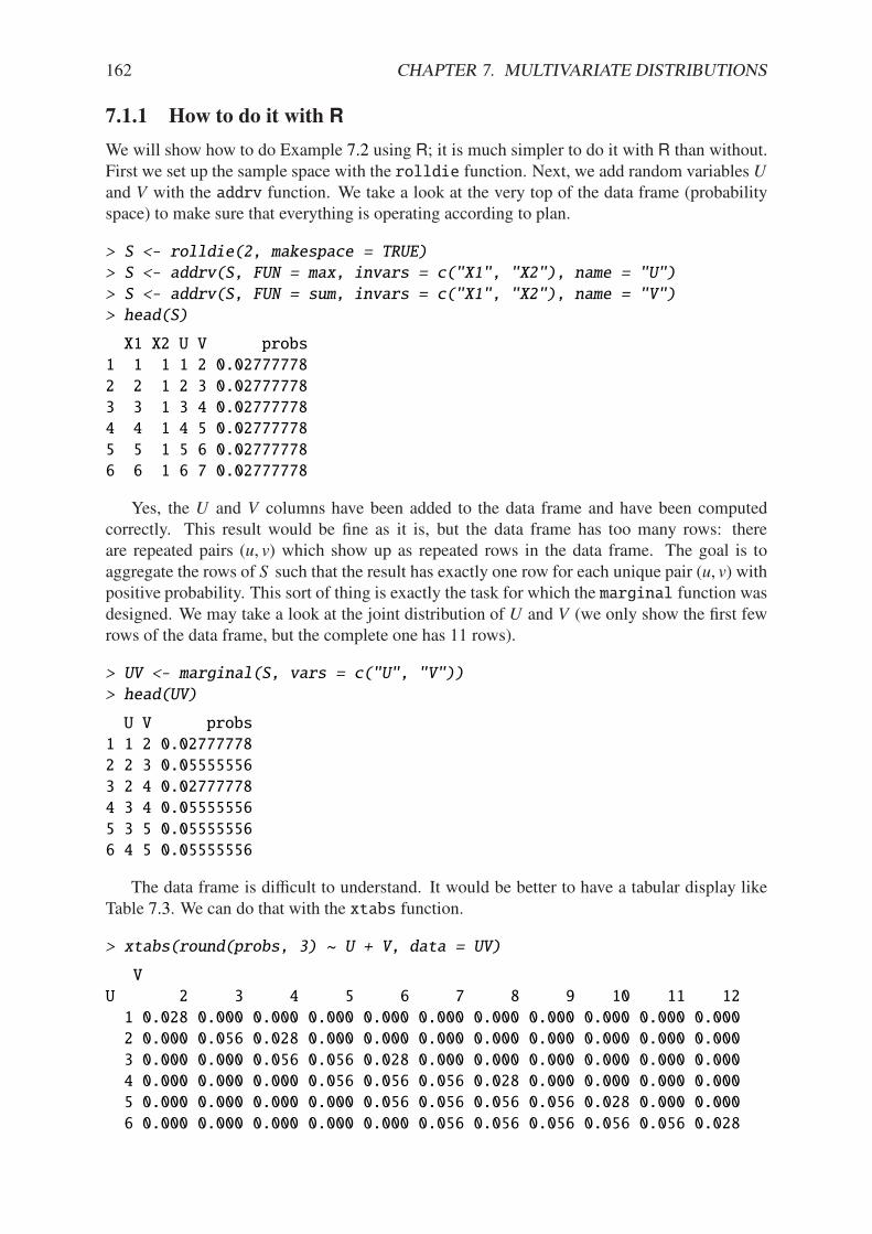
162 CHAPTER 7. MULTIVARIATE DISTRIBUTIONS
7.1.1 How to do it with R
We will show how to do Example 7.2 using R; it is much simpler to do it with R than without.First we set up the sample space with the rolldie function. Next, we add random variables Uand V with the addrv function. We take a look at the very top of the data frame (probabilityspace) to make sure that everything is operating according to plan.
> S <- rolldie(2, makespace = TRUE)
> S <- addrv(S, FUN = max, invars = c("X1", "X2"), name = "U")
> S <- addrv(S, FUN = sum, invars = c("X1", "X2"), name = "V")
> head(S)
X1 X2 U V probs
1 1 1 1 2 0.02777778
2 2 1 2 3 0.02777778
3 3 1 3 4 0.02777778
4 4 1 4 5 0.02777778
5 5 1 5 6 0.02777778
6 6 1 6 7 0.02777778
Yes, the U and V columns have been added to the data frame and have been computedcorrectly. This result would be fine as it is, but the data frame has too many rows: thereare repeated pairs (u, v) which show up as repeated rows in the data frame. The goal is toaggregate the rows of S such that the result has exactly one row for each unique pair (u, v) withpositive probability. This sort of thing is exactly the task for which the marginal function wasdesigned. We may take a look at the joint distribution of U and V (we only show the first fewrows of the data frame, but the complete one has 11 rows).
> UV <- marginal(S, vars = c("U", "V"))
> head(UV)
U V probs
1 1 2 0.02777778
2 2 3 0.05555556
3 2 4 0.02777778
4 3 4 0.05555556
5 3 5 0.05555556
6 4 5 0.05555556
The data frame is di"cult to understand. It would be better to have a tabular display likeTable 7.3. We can do that with the xtabs function.
> xtabs(round(probs, 3) ~ U + V, data = UV)
V
U 2 3 4 5 6 7 8 9 10 11 12
1 0.028 0.000 0.000 0.000 0.000 0.000 0.000 0.000 0.000 0.000 0.000
2 0.000 0.056 0.028 0.000 0.000 0.000 0.000 0.000 0.000 0.000 0.000
3 0.000 0.000 0.056 0.056 0.028 0.000 0.000 0.000 0.000 0.000 0.000
4 0.000 0.000 0.000 0.056 0.056 0.056 0.028 0.000 0.000 0.000 0.000
5 0.000 0.000 0.000 0.000 0.056 0.056 0.056 0.056 0.028 0.000 0.000
6 0.000 0.000 0.000 0.000 0.000 0.056 0.056 0.056 0.056 0.056 0.028

7.2. JOINT AND MARGINAL EXPECTATION 163
Compare these values to the ones shown in Table 7.3. We can repeat the process withmarginal to get the univariate marginal distributions of U and V separately.
> marginal(UV, vars = "U")
U probs
1 1 0.02777778
2 2 0.08333333
3 3 0.13888889
4 4 0.19444444
5 5 0.25000000
6 6 0.30555556
> head(marginal(UV, vars = "V"))
V probs
1 2 0.02777778
2 3 0.05555556
3 4 0.08333333
4 5 0.11111111
5 6 0.13888889
6 7 0.16666667
Another way to do the same thing is with the rowSums and colSums of the xtabs object.Compare
> temp <- xtabs(probs ~ U + V, data = UV)
> rowSums(temp)
1 2 3 4 5 6
0.02777778 0.08333333 0.13888889 0.19444444 0.25000000 0.30555556
> colSums(temp)
2 3 4 5 6 7
0.02777778 0.05555556 0.08333333 0.11111111 0.13888889 0.16666667
8 9 10 11 12
0.13888889 0.11111111 0.08333333 0.05555556 0.02777778
You should check that the answers that we have obtained exactly match the same (somewhatlaborious) calculations that we completed in Example 7.2.
7.2 Joint and Marginal Expectation
Given a function g with arguments (x, y) we would like to know the long-run average behaviorof g(X, Y) and how to mathematically calculate it. Expectation in this context is computed inthe pedestrian way. We simply integrate (sum) with respect to the joint probability density(mass) function.
IE g(X, Y) =
"S X,Y
g(x, y) fX,Y(x, y) dx dy, (7.2.1)
or in the discrete caseIE g(X, Y) =
! !
(x,y)3S X,Y
g(x, y) fX,Y(x, y). (7.2.2)
164 CHAPTER 7. MULTIVARIATE DISTRIBUTIONS
7.2.1 Covariance and Correlation
There are two very special cases of joint expectation: the covariance and the correlation. Theseare measures which help us quantify the dependence between X and Y .
Definition 7.4. The covariance of X and Y is
Cov(X, Y) = IE(X # IE X)(Y # IE Y). (7.2.3)
By the way, there is a shortcut formula for covariance which is almost as handy as theshortcut for the variance:
Cov(X, Y) = IE(XY) # (IE X)(IE Y). (7.2.4)
The proof is left to Exercise 7.1.The Pearson product moment correlation between X and Y is the covariance between X and
Y rescaled to fall in the interval [#1, 1]. It is formally defined by
Corr(X, Y) =Cov(X, Y)
"X"Y
(7.2.5)
The correlation is usually denoted by +X,Y or simply + if the random variables are clear fromcontext. There are some important facts about the correlation coe"cient:
1. The range of correlation is #1 " +X,Y " 1.
2. Equality holds above (+X,Y = ±1) if and only if Y is a linear function of X with probabilityone.
Example 7.5. Wewill compute the covariance for the discrete distribution in Example 7.2. Theexpected value of U is
IEU =
6!
u=1
u fU(u) =6!
u=1
u2u # 1
36= 1
01
36
1+ 2
03
36
1+ · · · + 6
011
36
1=
161
36,
and the expected value of V is
IEV =
12!
v=2
v6 # |7 # v|
36= 2
01
36
1+ 3
02
36
1+ · · · + 12
01
36
1= 7,
and the expected value of UV is
IEUV =
6!
u=1
12!
v=2
uv fU,V(u, v) = 1 · 201
36
1+ 2 · 3
02
36
1+ · · · + 6 · 12
01
36
1=
308
9.
Therefore the covariance of (U,V) is
Cov(U,V) = IEUV # (IEU) (IEV) =308
9#161
36· 7 =
35
12.
All we need now are the standard deviations of U and V to calculate the correlation coe"cient(omitted).
We will do a continuous example so that you can see how it works.
7.3. CONDITIONAL DISTRIBUTIONS 165
Example 7.6. Let us find the covariance of the variables (X, Y) from Example 7.3. The expectedvalue of X is
IE X =
B 1
0
x ·6
5
0x +
1
3
1dx =
2
5x3 +
1
5x2
444441
x=0=
3
5,
and the expected value of Y is
IE Y =
B 1
0
y ·6
5
01
2+ y2
1dx =
3
10y2 +
3
20y4
444441
y=0=
9
20.
Finally, the expected value of XY is
IE XY =
B 1
0
B 1
0
xy6
5
2x + y2
3dx dy,
=
B 1
0
02
5x3y +
3
10xy4
1444444
1
x=0
dy,
=
B 1
0
02
5y +
3
10y4
1dy,
=1
5+
3
50,
which is 13/50. Therefore the covariance of (X, Y) is
Cov(X, Y) =13
50#
03
5
1 09
20
1= #
1
100.
7.2.2 How to do it with R
There are not any specific functions in the prob package designed for multivariate expectation.This is not a problem, though, because it is easy enough to do expectation the long way – withcolumn operations. We just need to keep the definition in mind. For instance, we may computethe covariance of (U,V) from Example 7.5.
> Eu <- sum(S$U * S$probs)
> Ev <- sum(S$V * S$probs)
> Euv <- sum(S$U * S$V * S$probs)
> Euv - Eu * Ev
[1] 2.916667
Compare this answer to what we got in Example 7.5.To do the continuous case we could use the computer algebra utilities of Yacas and the
associated R package Ryacas [35]. See Section 7.7.1 for another example where the Ryacaspackage appears.
7.3 Conditional Distributions
If x 3 S X is such that fX(x) > 0, then we define the conditional density of Y | X = x, denotedfY |x, by
fY |x(y|x) =fX,Y(x, y)
fX(x), y 3 S Y . (7.3.1)
We define fX|y in a similar fashion.
166 CHAPTER 7. MULTIVARIATE DISTRIBUTIONS
Example 7.7. Let the joint PMF of X and Y be given by
fX,Y(x, y) =
Example 7.8. Let the joint PDF of X and Y be given by
Bayesian Connection
Conditional distributions play a fundamental role in Bayesian probability and statistics. Thereis a parameter , which is of primary interest, and about which we would like to learn. Butrather than observing , directly, we instead observe a random variable X whose probabilitydistribution depends on ,. Using the information we provided by X, we would like to updatethe information that we have about ,.
Our initial beliefs about , are represented by a probability distribution, called the prior dis-tribution, denoted by &. The PDF fX|, is called the likelihood function, also called the likelihoodof X conditional on ,. Given an observation X = x, we would like to update our beliefs & toa new distribution, called the posterior distribution of , given the observation X = x, denoted&,|x. It may seem a mystery how to obtain &,|x based only on the information provided by &and fX|,, but it should not be. We have already studied this in Section 4.8 where it was calledBayes’ Rule:
&(,|x) =&(,) f (x|,)A&(u) f (x|u)du
. (7.3.2)
Compare the above expression to Equation 4.8.1.
Example 7.9. Suppose the parameter , is the IP(Heads) for a biased coin. It could be any valuefrom 0 to 1. Perhaps we have some prior information about this coin, for example, maybe wehave seen this coin before and we have reason to believe that it shows Heads less than half ofthe time. Suppose that we represent our beliefs about , with a beta(shape1 = 1, shape2 = 3)prior distribution, that is, we assume
, 4 &(,) = 3(1 # ,)2, 0 < , < 1.
To learn more about ,, we will do what is natural: flip the coin. We will observe a ran-dom variable X which takes the value 1 if the coin shows Heads, and 0 if the coin showsTails. Under these circumstances, X will have a Bernoulli distribution, and in particular,X|, 4 binom(size = 1, prob = ,):
fX|,(x|,) = ,x(1 # ,)1#x, x = 0, 1.
Based on the observation X = x, we will update the prior distribution to the posterior distribu-tion, and we will do so with Bayes’ Rule: it says
&(,|x) % &(,) f (x|,),= ,x(1 # ,)1#x · 3(1 # ,)2,= 3 ,x(1 # ,)3#x, 0 < , < 1,
where the constant of proportionality is given by
B3 ux(1 # u)3#xdu =
B3 u(1+x)#1(1 # u)(4#x)#1du = 3
%(1 + x)%(4 # x)
%[(1 + x) + (4 # x)],
7.4. INDEPENDENT RANDOM VARIABLES 167
the integral being calculated by inspection of the formula for a beta(shape1 = 1+x, shape2 =4 # x) distribution. That is to say, our posterior distribution is precisely
,|x 4 beta(shape1 = 1 + x, shape2 = 4 # x).
The Bayesian statistician uses the posterior distribution for all matters concerning inferenceabout ,.
Remark 7.10. We usually do not restrict ourselves to the observation of only one X condi-tional on ,. In fact, it is common to observe an entire sample X1, X2,. . . ,Xn conditional on ,(which itself is often multidimensional). Do not be frightened, however, because the intuitionis the same. There is a prior distribution &(,), a likelihood f (x1, x2, . . . , xn|,), and a posteriordistribution &(,|x1, x2, . . . , xn). Bayes’ Rule states that the relationship between the three is
&(,|x1, x2, . . . , xn) % &(,) f (x1, x2, . . . , xn|,),
where the constant of proportionality isA&(u) f (x1, x2, . . . , xn|u) du. Any good textbook on
Bayesian Statistics will explain these notions in detail; to the interested reader I recommendGelman [33] or Lee [57].
7.4 Independent Random Variables
7.4.1 Independent Random Variables
We recall from Chapter 4 that the events A and B are said to be independent when
IP(A + B) = IP(A) IP(B). (7.4.1)
If it happens that
IP(X = x, Y = y) = IP(X = x) IP(Y = y), for every x 3 S X, y 3 S Y , (7.4.2)
then we say that X and Y are independent random variables. Otherwise, we say that X and Y
are dependent. Using the PMF notation from above, we see that independent discrete randomvariables satisfy
fX,Y(x, y) = fX(x) fY (y) for every x 3 S X, y 3 S Y . (7.4.3)
Continuing the reasoning, given two continuous random variables X and Y with joint PDF fX,Yand respective marginal PDFs fX and fY that are supported on the sets S X and S Y , if it happensthat
fX,Y(x, y) = fX(x) fY (y) for every x 3 S X, y 3 S Y , (7.4.4)
then we say that X and Y are independent.
Example 7.11. In Example 7.1 we considered the random experiment of rolling a fair die twice.There we found the joint PMF to be
fX,Y(x, y) =1
36, x = 1, . . . , 6, y = 1, . . . , 6,
and we found the marginal PMFs fX(x) = 1/6, x = 1, 2, . . . , 6, and fY(y) = 1/6, y = 1, 2, . . . , 6.Therefore in this experiment X and Y are independent since for every x and y in the joint supportthe joint PMF satisfies
fX,Y(x, y) =1
36=
01
6
1 01
6
1= fX(x) fY(y).

168 CHAPTER 7. MULTIVARIATE DISTRIBUTIONS
Example 7.12. In Example 7.2 we considered the same experiment but di!erent random vari-ables U and V . We can prove that U and V are not independent if we can find a single pair(u, v) where the independence equality does not hold. There are many such pairs. One of themis (6, 12):
fU,V(6, 12) =1
36!
011
36
1 01
36
1= fU(6) fV(12).
Independent random variables are very useful to the mathematician. They have many, many,tractable properties. We mention some of the more important ones.
Proposition 7.13. If X and Y are independent, then for any functions u and v,
IE (u(X)v(Y)) = (IE u(X)) (IE v(Y)) . (7.4.5)
Proof. This is straightforward from the definition.
IE (u(X)v(Y)) =
"u(x)v(y) fX,Y(x, y) dxdy
=
"u(x)v(y) fX(x) fY (y) dxdy
=
Bu(x) fX(x) dx
Bv(y) fY(y) dy
and this last quantity is exactly (IE u(X)) (IE v(Y)). "
Now that we have Proposition 7.13 we mention a corollary that will help us later to quicklyidentify those random variables which are not independent.
Corollary 7.14. If X and Y are independent, then Cov(X, Y) = 0, and consequently, Corr(X, Y) =0.
Proof. When X and Y are independent then IE XY = IE X IE Y . And when the covariance iszero the numerator of the correlation is 0. "
Remark 7.15. Unfortunately, the converse of Corollary 7.14 is not true. That is, there are manyrandom variables which are dependent yet their covariance and correlation is zero. For moredetails, see Casella and Berger [13].
Proposition 7.13 is useful to us and we will receive mileage out of it, but there is another factwhich will play an even more important role. Unfortunately, the proof is beyond the techniquespresented here. The inquisitive reader should consult Casella and Berger [13], Resnick [70],etc.
Fact 7.16. If X and Y are independent, then u(X) and v(Y) are independent for any functions uand v.
7.4.2 Combining Independent Random Variables
Another important corollary of Proposition 7.13 will allow us to find the distribution of sumsof random variables.
Corollary 7.17. If X and Y are independent, then the moment generating function of X + Y is
MX+Y(t) = MX(t) · MY(t). (7.4.6)
7.4. INDEPENDENT RANDOM VARIABLES 169
Proof. Choose u(x) = ex and v(y) = ey in Proposition 7.13, and remember the identity et(x+y) =etx ety. "
Let us take a look at some examples of the corollary in action.
Example 7.18. Let X 4 binom(size = n1, prob = p) and Y 4 binom(size = n2, prob = p)be independent. Then X + Y has MGF
MX+Y(t) = MX(t)MY(t) ==q + pet
>n1 =q + pet
>n2 ==q + pet
>n1+n2 ,
which is the MGF of a binom(size = n1 + n2, prob = p) distribution. Therefore, X + Y 4binom(size = n1 + n2, prob = p).
Example 7.19. Let X 4 norm(mean = µ1, sd = "1) and Y 4 norm(mean = µ2, sd = "2) beindependent. Then X + Y has MGF
MX(t)MY(t) = exp5µ1t + t
2"21/2
6exp
5µ2t + t
2"22/2
6= exp
5(µ1 + µ2) t + t
22"2
1 + "22
3/2
6,
which is the MGF of a norm(mean = µ1 + µ2, sd =M"2
1 + "22) distribution.
Even when we cannot use the MGF trick to identify the exact distribution of a linear com-bination of random variables, we can still say something about its mean and variance.
Proposition 7.20. Let X1 and X2 be independent with respective population means µ1 and µ2and population standard deviations "1 and "2. For given constants a1 and a2, define Y =
a1X1 + a2X2. Then the mean and standard deviation of Y are given by the formulas
µY = a1µ1 + a2µ2, "Y =2a21"
21 + a
22"
22
31/2. (7.4.7)
Proof. We use Proposition 5.11:
IE Y = IE (a1X1 + a2X2) = a1 IE X1 + a2 IE X2 = a1µ1 + a2µ2.
For the standard deviation, we will find the variance and take the square root at the end. Andto calculate the variance we will first compute IE Y2 with an eye toward using the identity"2
Y = IE Y2 # (IE Y)2 as a final step.
IE Y2 = IE (a1X1 + a2X2)2 = IE
2a21X
21 + a
22X
22 + 2a1a2X1X2
3.
Using linearity of expectation the IE distributes through the sum. Now IE X2i = "
2i + µ
2i , for
i = 1 and 2 and IE X1X2 = IE X1 IE X2 = µ1µ2 because of independence. Thus
IE Y2 = a21("21 + µ
21) + a
22("
22 + µ
22) + 2a1a2µ1µ2,
= a21"21 + a
22"
22 +
2a21µ
21 + a
22µ
22 + 2a1a2µ1µ2
3.
But notice that the expression in the parentheses is exactly (a1µ1 + a2µ2)2 = (IE Y)2, so the
proof is complete.. "
170 CHAPTER 7. MULTIVARIATE DISTRIBUTIONS
7.5 Exchangeable Random Variables
Two random variables X and Y are said to be exchangeable if their joint CDF is a symmetricfunction of its arguments:
FX,Y(x, y) = FX,Y(y, x), for all (x, y) 3 R2. (7.5.1)
When the joint density f exists, we may equivalently say that X and Y are exchangeable iff (x, y) = f (y, x) for all (x, y).
Exchangeable random variables exhibit symmetry in the sense that a person may exchangeone variable for the other with no substantive changes to their joint random behavior. Whileindependence speaks to a lack of influence between the two variables, exchangeability aims tocapture the symmetry between them.
Example 7.21. Let X and Y have joint PDF
fX,Y(x, y) = (1 + ()%2e#%(x+y) + ((2%)2e#2%(x+y) # 2(%22e#%(2x+y) + e#%(x+2y)
3. (7.5.2)
It is straightforward and tedious to check that#
f = 1. Wemay see immediately that fX,Y(x, y) =fX,Y(y, x) for all (x, y), which confirms that X and Y are exchangeable. Here, ( is said to be anassociation parameter. This particular example is one from the Farlie-Gumbel-Morgensternfamily of distributions; see [54].
Example 7.22. Suppose X and Y are i.i.d. binom(size = n, prob = p). Then their joint PMFis
fX,Y(x, y) = fX(x) fY (y)
=
0n
x
1px(1 # p)n#x
0n
y
1py(1 # p)n#y,
=
0n
x
10n
y
1px+y(1 # p)2n#(x+y) ,
and the value is the same if we exchange x and y. Therefore (X, Y) are exchangeable.
Looking at Example 7.22 more closely we see that the fact that (X, Y) are exchangeablehas nothing to do with the binom(size = n, prob = p) distribution; it only matters that theyare independent (so that the joint PDF factors) and they are identically distributed (in whichcase we may swap letters to no e!ect). We could just have easily used any other marginaldistribution. We will take this as a proof of the following proposition.
Proposition 7.23. If X and Y are i.i.d. (with common marginal distribution F) then X and Y
are exchangeable.
Exchangeability thus contains i.i.d. as a special case.
7.6 The Bivariate Normal Distribution
The bivariate normal PDF is given by the unwieldy formula
fX,Y(x, y) =1
2&"X"Y
N1 # +2
exp
9::;::<#
1
2(1 # +2)
EFFFFG0x # µX"X
12+ · · ·
· · · + 2+0x # µX"X
1 0y # µY"Y
1+
0y # µY"Y
12HIIIIJ
O::P::Q , (7.6.1)
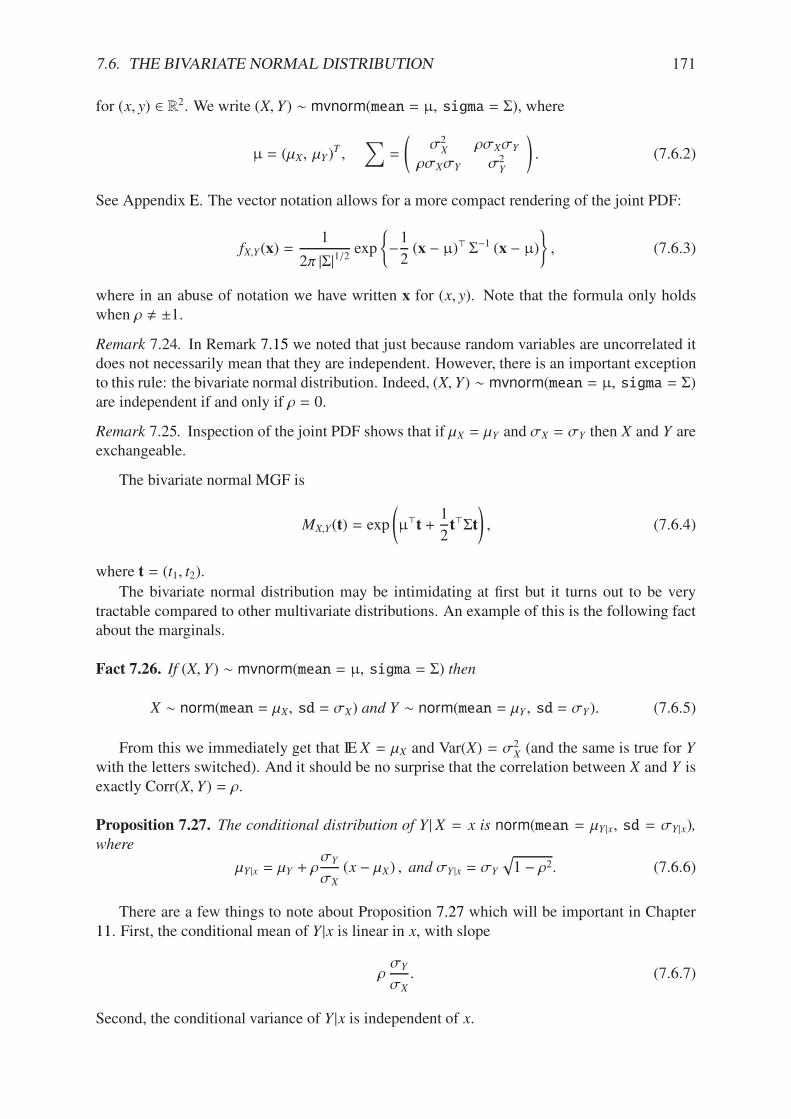
7.6. THE BIVARIATE NORMAL DISTRIBUTION 171
for (x, y) 3 R2. We write (X, Y) 4 mvnorm(mean = µ, sigma = &), where
µ = (µX, µY)T ,
!=
0"2
X +"X"Y
+"X"Y "2Y
1. (7.6.2)
See Appendix E. The vector notation allows for a more compact rendering of the joint PDF:
fX,Y(x) =1
2& |&|1/2exp
.#1
2(x # µ)8  (x # µ)
/, (7.6.3)
where in an abuse of notation we have written x for (x, y). Note that the formula only holdswhen + ! ±1.
Remark 7.24. In Remark 7.15 we noted that just because random variables are uncorrelated itdoes not necessarily mean that they are independent. However, there is an important exceptionto this rule: the bivariate normal distribution. Indeed, (X, Y) 4 mvnorm(mean = µ, sigma = &)are independent if and only if + = 0.
Remark 7.25. Inspection of the joint PDF shows that if µX = µY and "X = "Y then X and Y areexchangeable.
The bivariate normal MGF is
MX,Y(t) = exp
0µ8t +
1
2t8&t
1, (7.6.4)
where t = (t1, t2).
The bivariate normal distribution may be intimidating at first but it turns out to be verytractable compared to other multivariate distributions. An example of this is the following factabout the marginals.
Fact 7.26. If (X, Y) 4 mvnorm(mean = µ, sigma = &) then
X 4 norm(mean = µX, sd = "X) and Y 4 norm(mean = µY , sd = "Y). (7.6.5)
From this we immediately get that IE X = µX and Var(X) = "2X (and the same is true for Y
with the letters switched). And it should be no surprise that the correlation between X and Y isexactly Corr(X, Y) = +.
Proposition 7.27. The conditional distribution of Y | X = x is norm(mean = µY |x, sd = "Y |x),where
µY |x = µY + +"Y
"X
(x # µX) , and "Y |x = "Y
N1 # +2. (7.6.6)
There are a few things to note about Proposition 7.27 which will be important in Chapter11. First, the conditional mean of Y |x is linear in x, with slope
+"Y
"X
. (7.6.7)
Second, the conditional variance of Y |x is independent of x.
172 CHAPTER 7. MULTIVARIATE DISTRIBUTIONS
7.6.1 How to do it with R
The multivariate normal distribution is implemented in both the mvtnorm package [34] andthe mnormt package [17]. We use the mvtnorm package in this book simply because it is adependency of another package used in the book.
The mvtnorm package has functions dmvnorm and rmvnorm for the PDF and to generaterandom vectors, respectively. Let us get started with a graph of the bivariate normal PDF. Wecan make the plot with the following code3, where the workhorse is the persp function in baseR.
> library(mvtnorm)
> x <- y <- seq(from = -3, to = 3, length.out = 30)
> f <- function(x, y) dmvnorm(cbind(x, y), mean = c(0, 0),
+ sigma = diag(2))
> z <- outer(x, y, FUN = f)
> persp(x, y, z, theta = -30, phi = 30, ticktype = "detailed")
We chose the standard bivariate normal, mvnorm(mean = 0, sigma = I), to display.
7.7 Bivariate Transformations of Random Variables
We studied in Section 6.4 how to find the PDF of Y = g(X) given the PDF of X. But now wehave two random variables X and Y, with joint PDF fX,Y, and we would like to consider thejoint PDF of two new random variables
U = g(X, Y) and V = h(X, Y), (7.7.1)
where g and h are two given functions, typically “nice” in the sense of Appendix E.6.Suppose that the transformation (x, y) 9#. (u, v) is one-to-one. Then an inverse transforma-
tion x = x(u, v) and y = y(u, v) exists, so let -(x, y)/-(u, v) denote the Jacobian of the inversetransformation. Then the joint PDF of (U,V) is given by
fU,V(u, v) = fX,YRx(u, v), y(u, v)
S 44444-(x, y)
-(u, v)
44444 , (7.7.2)
or we can rewrite more shortly as
fU,V(u, v) = fX,Y(x, y)
44444-(x, y)
-(u, v)
44444 . (7.7.3)
Take a moment and compare Equation 7.7.3 to Equation 6.4.2. Do you see the connection?
3Another way to do this is with the curve3d function in the emdbook package [9]. It looks like this:
library(emdbook); library(mvtnorm) # note: the order matters
mu <- c(0,0); sigma <- diag(2)
f <- function(x,y) dmvnorm(c(x,y), mean = mu, sigma = sigma)
curve3d(f(x,y), from = c(-3,-3), to = c(3,3), theta = -30, phi = 30)
The code above is slightly shorter than that using persp and is easier to understand. One must be careful, however.If the library calls are swapped then the code will not work because both packages emdbook and mvtnorm havea function called “dmvnorm”; one must load them to the search path in the correct order or R will use the wrongone (the arguments are named di!erently and the underlying algorithms are di!erent).
7.7. BIVARIATE TRANSFORMATIONS OF RANDOM VARIABLES 173
x
!3
!2
!1
01
23
y
!3
!2
!1
0
1
2
3z
0.05
0.10
0.15
Figure 7.6.1: Graph of a bivariate normal PDF
174 CHAPTER 7. MULTIVARIATE DISTRIBUTIONS
Remark 7.28. It is sometimes easier to postpone solving for the inverse transformation x =
x(u, v) and y = y(u, v). Instead, leave the transformation in the form u = u(x, y) and v = v(x, y)and calculate the Jacobian of the original transformation
-(u, v)
-(x, y)=
444444
-u-x
-u-y
-v-x
-v-y
444444 =-u
-x
-v
-y#-u
-y
-v
-x. (7.7.4)
Once this is known, we can get the PDF of (U,V) by
fU,V(u, v) = fX,Y(x, y)
44444441-(u,v)-(x,y)
4444444. (7.7.5)
In some cases there will be a cancellation and the work will be a lot shorter. Of course, it is notalways true that
-(x, y)
-(u, v)=
1-(u,v)-(x,y)
, (7.7.6)
but for the well-behaved examples that we will see in this book it works just fine. . . do you seethe connection between Equations 7.7.6 and 6.4.5?
Example 7.29. Let (X, Y) 4 mvnorm(mean = 0271, sigma = I272) and consider the transfor-mation
U = 3X + 4Y,
V = 5X + 6Y.
We can solve the system of equations to find the inverse transformations; they are
X = # 3U + 2V,
Y =5
2U #
3
2V,
in which case the Jacobian of the inverse transformation is444444#3 252
#32
444444 = 3
0#3
2
1# 2
05
2
1= #
1
2.
As (x, y) traverses R2, so too does (u, v). Since the joint PDF of (X, Y) is
fX,Y(x, y) =1
2&exp
.#1
2
2x2 + y2
3/, (x, y) 3 R2,
we get that the joint PDF of (U,V) is
fU,V(u, v) =1
2&exp
9::;::<#
1
2
EFFFFG(#3u + 2v)2 +
05u # 3v
2
12HIIIIJ
O::P::Q ·
1
2, (u, v) 3 R2. (7.7.7)
Remark 7.30. It may not be obvious, but Equation 7.7.7 is the PDF of a mvnorm distribution.For a more general result see Theorem 7.34.
7.8. REMARKS FOR THE MULTIVARIATE CASE 175
7.7.1 How to do it with R
It is possible to do the computations above in R with the Ryacas package. The package is aninterface to the open-source computer algebra system, “Yacas”. The user installs Yacas, thenemploys Ryacas to submit commands to Yacas, after which the output is displayed in the Rconsole.
There are not yet any examples of Yacas in this book, but there are online materials to helpthe interested reader: see http://code.google.com/p/ryacas/ to get started.
7.8 Remarks for the Multivariate Case
There is nothing spooky about n / 3 random variables. We just have a whole bunch of them:X1, X2,. . . , Xn, which we can shorten to X = (X1, X2, . . . , Xn)
T to make the formulas prettier(now may be a good time to check out Appendix E.5). For X supported on the set S X, the jointPDF fX (if it exists) satisfies
fX(x) > 0, for x 3 S X, (7.8.1)
and BB· · ·
BfX(x) dx1dx2 · · · dxn = 1, (7.8.2)
or even shorter:AfX(x) dx = 1. The joint CDF FX is defined by
FX(x) = IP(X1 " x1, X2 " x2, . . . , Xn " xn), (7.8.3)
for x 3 Rn. The expectation of a function g(X) is defined just as we would imagine:
IE g(X) =
Bg(x) fX(x) dx. (7.8.4)
provided the integral exists and is finite. And the moment generating function in the multivari-ate case is defined by
MX(t) = IE exp5tTX
6, (7.8.5)
whenever the integral exists and is finite for all t in a neighborhood of 0n71 (note that tTX isshorthand for t1X1 + t2X2 + · · · + tnXn). The only di!erence in any of the above for the discretecase is that integrals are replaced by sums.
Marginal distributions are obtained by integrating out remaining variables from the jointdistribution. And even if we are given all of the univariate marginals it is not enough to deter-mine the joint distribution uniquely.
We say that X1, X2, . . . , Xn are mutually independent if their joint PDF factors into theproduct of the marginals
fX(x) = fX1(x1) fX2(x2) · · · fXn(xn), (7.8.6)
for every x in their joint support S X, and we say that X1, X2, . . . , Xn are exchangeable if theirjoint PDF (or CDF) is a symmetric function of its n arguments, that is, if
fX(x6) = fX(x), (7.8.7)
for any reordering x6 of the elements of x = (x1, x2, . . . , xn) in the joint support.
176 CHAPTER 7. MULTIVARIATE DISTRIBUTIONS
Proposition 7.31. Let X1, X2, . . . , Xn be independent with respective population means µ1,
µ2, . . . , µn and standard deviations "1, "2, . . . , "n. For given constants a1, a2, . . . ,an define
Y =#n
i=1 aiXi. Then the mean and standard deviation of Y are given by the formulas
µY =
n!
i=1
aiµi, "Y =
$%%%%%&
n!
i=1
a2i"2i
()))))*
1/2
. (7.8.8)
Proof. The mean is easy:
IE Y = IE
$%%%%%&
n!
i=1
aiXi
()))))* =
n!
i=1
ai IE Xi =
n!
i=1
aiµi.
The variance is not too di"cult to compute either. As an intermediate step, we calculate IE Y2.
IE Y2 = IE
$%%%%%&
n!
i=1
aiXi
()))))*
2
= IE
$%%%%%%&
n!
i=1
a2i X2i + 2
n#1!
i=1
n!
j=i+1
aia jXiX j
())))))* .
Using linearity of expectation the IE distributes through the sums. Now IE X2i = "
2i + µ
2i and
IE XiXj = IE Xi IE Xj = µiµ j when i ! j because of independence. Thus
IE Y2 =
n!
i=1
a2i ("2i + µ
2i ) + 2
n#1!
i=1
n!
j=i+1
aia jµiµ j
=
n!
i=1
a2i"2i +
$%%%%%%&
n!
i=1
a2i µ2i + 2
n#1!
i=1
n!
j=i+1
aia jµiµ j
())))))*
To complete the proof, note that the expression in the parentheses is exactly (IE Y)2, and recallthe identity "2
Y = IE Y2 # (IE Y)2. "
There is a corresponding statement of Fact 7.16 for the multivariate case. The proof is alsoomitted here.
Fact 7.32. If X and Y are mutually independent random vectors, then u(X) and v(Y) are inde-pendent for any functions u and v.
Bruno de Finetti was a strong proponent of the subjective approach to probability. Heproved an important theorem in 1931 which illuminates the link between exchangeable randomvariables and independent random variables. Here it is in one of its simplest forms.
Theorem 7.33. De Finetti’s Theorem. Let X1, X2, . . . be a sequence of binom(size =1, prob = p) random variables such that (X1, . . . , Xk) are exchangeable for every k. Then
there exists a random variable ' with support [0, 1] and PDF f'(,) such that
IP(X1 = x1, . . . , Xk = xk) =
B 1
0
,#
xi(1 # ,)k##
xi f'(,) d,, (7.8.9)
for all xi = 0, 1, i = 1, 2, . . . , k.
7.8. REMARKS FOR THE MULTIVARIATE CASE 177
To get a handle on the intuitive content de Finetti’s theorem, imagine that we have a bunchof coins in our pocket with each having its own unique value of , = IP(Heads). We reach intoour pocket and select a coin at random according to some probability – say, f'(,). We take therandomly selected coin and flip it k times.
Think carefully: the conditional probability of observing a sequence X1 = x1, . . . , Xk = xk,given a specific coin , would just be ,
#xi(1 # ,)k#
#xi , because the coin flips are an independent
sequence of Bernoulli trials. But the coin is random, so the Theorem of Total Probability sayswe can get the unconditional probability IP(X1 = x1, . . . , Xk = xk) by adding up terms that looklike
,#
xi(1 # ,)k##
xi f'(,), (7.8.10)
where we sum over all possible coins. The right-hand side of Equation 7.8.9 is a sophisticatedway to denote this process.
Of course, the integral’s value does not change if we jumble the xi’s, so (X1, . . . , Xk) areclearly exchangeable. The power of de Finetti’s Theorem is that every infinite binary exchange-able sequence can be written in the above form.
The connection to subjective probability: our prior information about , corresponds tof'(,) and the likelihood of the sequence X1 = x1, . . . , Xk = xk (conditional on ,) correspondsto ,
#xi(1 # ,)k#
#xi . Compare Equation 7.8.9 to Section 4.8 and Section 7.3.
The multivariate normal distribution immediately generalizes from the bivariate case. If thematrix & is nonsingular then the joint PDF of X 4 mvnorm(mean = µ, sigma = &) is
fX(x) =1
(2&)n/2 |&|1/2exp
.#1
2(x # µ)8  (x # µ)
/, (7.8.11)
and the MGF is
MX(t) = exp
.µ8t +
1
2t8&t
/. (7.8.12)
We will need the following in Chapter 12.
Theorem 7.34. If X 4 mvnorm(mean = µ, sigma = &) and A is any matrix, then the random
vector Y = AX is distributed
Y 4 mvnorm(mean = Aµ, sigma = A&AT). (7.8.13)
Proof. Look at the MGF of Y:
MY(t) = IE exp5tT(AX)
6,
= IE exp5(ATt)TX
6,
= exp
.µT(A8t) +
1
2(ATt)T&(ATt)
/,
= exp
.(Aµ)T t +
1
2tT
2A&AT
3t
/,
and the last expression is the MGF of an mvnorm(mean = Aµ, sigma = A&AT) distribution."
178 CHAPTER 7. MULTIVARIATE DISTRIBUTIONS
7.9 The Multinomial Distribution
We sample n times, with replacement, from an urn that contains balls of k di!erent types. LetX1 denote the number of balls in our sample of type 1, let X2 denote the number of balls of type2, . . . , and let Xk denote the number of balls of type k. Suppose the urn has proportion p1 ofballs of type 1, proportion p2 of balls of type 2, . . . , and proportion pk of balls of type k. Thenthe joint PMF of (X1, . . . , Xk) is
fX1,...,Xk(x1, . . . , xk) =
0n
x1 x2 · · · xk
1px11 px22 · · · p
xkk, (7.9.1)
for (x1, . . . , xk) in the joint support S X1,...XK. We write
(X1, . . . , Xk) 4 multinom(size = n, prob = pk71). (7.9.2)
Several comments are in order. First, the joint support set S X1,...XKcontains all nonnegative
integer k-tuples (x1, . . . , xk) such that x1 + x2 + · · · + xk = n. A support set like this is called asimplex. Second, the proportions p1, p2, . . . , pk satisfy pi / 0 for all i and p1+ p2+ · · ·+ pk = 1.Finally, the symbol 0
n
x1 x2 · · · xk
1=
n!
x1! x2! · · · xk!(7.9.3)
is called a multinomial coe!cient which generalizes the notion of a binomial coe"cient wesaw in Equation 4.5.1.
The form and notation we have just described matches the R usage but is not standardamong other texts. Most other books use the above for a k # 1 dimension multinomial distribu-tion, because the linear constraint x1 + x2 + · · · + xk = n means that once the values of X1, X2,. . . , Xk#1 are known the final value Xk is determined, not random. Another term used for this isa singular distribution.
For the most part we will ignore these di"culties, but the careful reader should keep themin mind. There is not much of a di!erence in practice, except that below we will use a two-dimensional support set for a three-dimension multinomial distribution. See Figure 7.9.1.
When k = 2, we have x1 = x and x2 = n # x, we have p1 = p and p2 = 1 # p, and themultinomial coe"cient is literally a binomial coe"cient. In the previous notation we have thusshown that the multinom(size = n, prob = p271) distribution is the same as a binom(size =n, prob = p) distribution.
Example 7.35. Dinner with Barack Obama. During the 2008 U.S. presidential primary, BarackObama o!ered to have dinner with three randomly selected monetary contributors to his cam-paign. Imagine the thousands of people in the contributor database. For the sake of argument,Suppose that the database was approximately representative of the U.S. population as a whole,Suppose Barack Obamawants to have dinner http://pewresearch.org/pubs/773/fewer-voters-ident36 democrat, 27 republican , 37 independent.
Remark 7.36. Here are some facts about the multinomial distribution.
1. The expected value of (X1, X2, . . . , Xk) is npk71.
2. The variance-covariance matrix & is symmetric with diagonal entries "2i = npi(1 # pi),
i = 1, 2, . . . , k and o!-diagonal entries Cov(Xi, Xj) = #npip j, for i ! j. The correlationbetween Xi and Xj is therefore Corr(Xi, Xj) = #
Npip j/(1 # pi)(1 # pj).
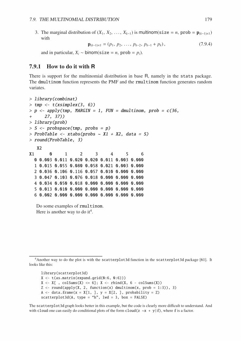
7.9. THE MULTINOMIAL DISTRIBUTION 179
3. The marginal distribution of (X1, X2, . . . , Xk#1) is multinom(size = n, prob = p(k#1)71)with
p(k#1)71 = (p1, p2, . . . , pk#2, pk#1 + pk) , (7.9.4)
and in particular, Xi 4 binom(size = n, prob = pi).
7.9.1 How to do it with R
There is support for the multinomial distribution in base R, namely in the stats package.The dmultinom function represents the PMF and the rmultinom function generates randomvariates.
> library(combinat)
> tmp <- t(xsimplex(3, 6))
> p <- apply(tmp, MARGIN = 1, FUN = dmultinom, prob = c(36,
+ 27, 37))
> library(prob)
> S <- probspace(tmp, probs = p)
> ProbTable <- xtabs(probs ~ X1 + X2, data = S)
> round(ProbTable, 3)
X2
X1 0 1 2 3 4 5 6
0 0.003 0.011 0.020 0.020 0.011 0.003 0.000
1 0.015 0.055 0.080 0.058 0.021 0.003 0.000
2 0.036 0.106 0.116 0.057 0.010 0.000 0.000
3 0.047 0.103 0.076 0.018 0.000 0.000 0.000
4 0.034 0.050 0.018 0.000 0.000 0.000 0.000
5 0.013 0.010 0.000 0.000 0.000 0.000 0.000
6 0.002 0.000 0.000 0.000 0.000 0.000 0.000
Do some examples of rmultinom.Here is another way to do it4.
4Another way to do the plot is with the scatterplot3d function in the scatterplot3d package [61]. Itlooks like this:
library(scatterplot3d)
X <- t(as.matrix(expand.grid(0:6, 0:6)))
X <- X[ , colSums(X) <= 6]; X <- rbind(X, 6 - colSums(X))
Z <- round(apply(X, 2, function(x) dmultinom(x, prob = 1:3)), 3)
A <- data.frame(x = X[1, ], y = X[2, ], probability = Z)
scatterplot3d(A, type = “h”, lwd = 3, box = FALSE)
The scatterplot3d graph looks better in this example, but the code is clearly more di"cult to understand. Andwith cloud one can easily do conditional plots of the form cloud(z ~x + y|f), where f is a factor.
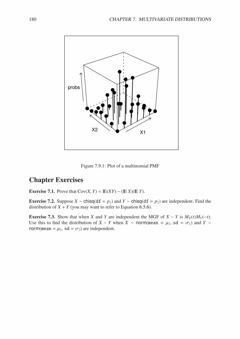
180 CHAPTER 7. MULTIVARIATE DISTRIBUTIONS
X1X2
probs
Figure 7.9.1: Plot of a multinomial PMF
Chapter Exercises
Exercise 7.1. Prove that Cov(X, Y) = IE(XY) # (IE X)(IE Y).
Exercise 7.2. Suppose X 4 chisq(df = p1) and Y 4 chisq(df = p2) are independent. Find thedistribution of X + Y (you may want to refer to Equation 6.5.6).
Exercise 7.3. Show that when X and Y are independent the MGF of X # Y is MX(t)MY(#t).Use this to find the distribution of X # Y when X 4 norm(mean = µ1, sd = "1) and Y 4norm(mean = µ2, sd = "2) are independent.
Chapter 8
Sampling Distributions
This is an important chapter; it is the bridge from probability and descriptive statistics that westudied in Chapters 3 through 7 to inferential statistics which forms the latter part of this book.
Here is the link: we are presented with a population about which we would like to learn.And while it would be desirable to examine every single member of the population, we findthat it is either impossible or infeasible to for us to do so, thus, we resort to collecting a sampleinstead. We do not lose heart. Our method will su"ce, provided the sample is representativeof the population. A good way to achieve this is to sample randomly from the population.
Supposing for the sake of argument that we have collected a random sample, the next task isto make some sense out of the data because the complete list of sample information is usuallycumbersome, unwieldy. We summarize the data set with a descriptive statistic, a quantitycalculated from the data (we saw many examples of these in Chapter 3). But our sample wasrandom. . . therefore, it stands to reason that our statistic will be random, too. How is thestatistic distributed?
The probability distribution associated with the population (from which we sample) iscalled the population distribution, and the probability distribution associated with our statisticis called its sampling distribution; clearly, the two are interrelated. To learn about the popu-lation distribution, it is imperative to know everything we can about the sampling distribution.Such is the goal of this chapter.
We begin by introducing the notion of simple random samples and cataloguing some of theirmore convenient mathematical properties. Next we focus on what happens in the special caseof sampling from the normal distribution (which, again, has several convenient mathematicalproperties), and in particular, we meet the sampling distribution of X and S 2. Then we explorewhat happens to X’s sampling distribution when the population is not normal and prove one ofthe most remarkable theorems in statistics, the Central Limit Theorem (CLT).
With the CLT in hand, we then investigate the sampling distributions of several other pop-ular statistics, taking full advantage of those with a tractable form. We finish the chapter withan exploration of statistics whose sampling distributions are not quite so tractable, and to ac-complish this goal we will use simulation methods that are grounded in all of our work in theprevious four chapters.
What do I want them to know?
• the notion of population versus simple random sample, parameter versus statistic, andpopulation distribution versus sampling distribution
• the classical sampling distributions of the standard one and two sample statistics
181
182 CHAPTER 8. SAMPLING DISTRIBUTIONS
• how to generate a simulated sampling distribution when the statistic is crazy
• the Central Limit Theorem, period.
• some basic concepts related to sampling distribution utility, such as bias and variance
8.1 Simple Random Samples
8.1.1 Simple Random Samples
Definition 8.1. If X1, X2, . . . , Xn are independent with Xi 4 f for i = 1, 2, . . . , n, then we saythat X1, X2, . . . , Xn are independent and identically distributed (i.i.d.) from the population f oralternatively we say that X1, X2, . . . , Xn are a simple random sample of size n, denoted SRS (n),from the population f .
Proposition 8.2. Let X1, X2, . . . , Xn be a SRS (n) from a population distribution with mean µ
and finite standard deviation ". Then the mean and standard deviation of X are given by the
formulas µX = µ and "X = "/$n.
Proof. Plug in a1 = a2 = · · · = an = 1/n in Proposition 7.31. "
The next fact will be useful to us when it comes time to prove the Central Limit Theoremin Section 8.3.
Proposition 8.3. Let X1, X2, . . . , Xn be a SRS (n) from a population distribution with MGF
M(t). Then the MGF of X is given by
MX(t) =KM
?t
n
@Ln. (8.1.1)
Proof. Go from the definition:
MX(t) = IE etX,
= IE et(X1+···+Xn)/n,
= IE etX1/netX2/n · · · etXn/n.
And because X1, X2, . . . , Xn are independent, Proposition 7.13 allows us to distribute the ex-pectation among each term in the product, which is
IE etX1/n IE etX2/n · · · IE etXn/n.
The last step is to recognize that each term in last product above is exactly M(t/n). "
8.2 Sampling from a Normal Distribution
8.2.1 The Distribution of the Sample Mean
Proposition 8.4. Let X1, X2, . . . , Xn be a SRS (n) from a norm(mean = µ, sd = ") distribution.Then the sample mean X has a norm(mean = µ, sd = "/
$n) sampling distribution.
8.2. SAMPLING FROM A NORMAL DISTRIBUTION 183
Proof. The mean and standard deviation of X follow directly from Proposition 8.2. To addressthe shape, first remember from Section 6.3 that the norm(mean = µ, sd = ") MGF is of theform
M(t) = exp5µt + "2t2/2
6.
Now use Proposition 8.3 to find
MX(t) =KM
?t
n
@Ln,
=Cexp
5µ(t/n) + "2(t/n)2/2
6Dn,
= exp5n ·
Cµ(t/n) + "2(t/n)2/2
D6,
= exp5µt + ("/
$n)2t2/2
6,
and we recognize this last quantity as the MGF of a norm(mean = µ, sd = "/$n) distribution.
"
8.2.2 The Distribution of the Sample Variance
Theorem 8.5. Let X1, X2, . . . , Xn be a SRS (n) from a norm(mean = µ, sd = ") distribution,and let
X =
n!
i=1
Xi and S 2 =1
n # 1
n!
i=1
(Xi # X)2. (8.2.1)
Then
1. X and S 2 are independent, and
2. The rescaled sample variance
(n # 1)
"2S 2 =
#ni=1(Xi # X)2
"2(8.2.2)
has a chisq(df = n # 1) sampling distribution.
Proof. The proof is beyond the scope of the present book, but the theorem is simply too impor-tant to be omitted. The interested reader could consult Casella and Berger [13], or Hogg et al
[43]. "
8.2.3 The Distribution of Student’s T Statistic
Proposition 8.6. Let X1, X2, . . . , Xn be a SRS (n) from a norm(mean = µ, sd = ") distribution.Then the quantity
T =X # µS/
$n
(8.2.3)
has a t(df = n # 1) sampling distribution.
Proof. Divide the numerator and denominator by " and rewrite
T =
X#µ"/
$n
S/"=
X#µ"/
$n
M(n#1)S 2
"2
T(n # 1)
.
184 CHAPTER 8. SAMPLING DISTRIBUTIONS
Now let
Z =X # µ"/
$n
and V =(n # 1)S 2
"2,
so that
T =Z
$V/r, (8.2.4)
where r = n # 1.We know from Section 8.2.1 that Z 4 norm(mean = 0, sd = 1) and we know from Section
8.2.2 that V 4 chisq(df = n # 1). Further, since we are sampling from a normal distribu-tion, Theorem 8.5 gives that X and S 2 are independent and by Fact 7.16 so are Z and V . Insummary, the distribution of T is the same as the distribution of the quantity Z/
$V/r, where
Z 4 norm(mean = 0, sd = 1) and V 4 chisq(df = r) are independent. This is in fact thedefinition of Student’s t distribution. "
This distribution was first published by W. S. Gosset (1900) under the pseudonym Student,and the distribution has consequently come to be known as Student’s t distribution. The PDFof T can be derived explicitly using the techniques of Section 6.4; it takes the form
fX(x) =%[(r + 1)/2]$r& %(r/2)
01 +
x2
r
1#(r+1)/2, #& < x < & (8.2.5)
Any random variable X with the preceding PDF is said to have Student’s t distributionwith rdegrees of freedom, and we write X 4 t(df = r). The shape of the PDF is similar to the normal,but the tails are considerably heavier. See Figure 8.2.1. As with the normal distribution, thereare four functions in R associated with the t distribution, namely dt, pt, qt, and rt, whichcompute the PDF, CDF, quantile function, and generate random variates, respectively.
The code to produce Figure 8.2.1 is
> curve(dt(x, df = 30), from = -3, to = 3, lwd = 3, ylab = "y")
> ind <- c(1, 2, 3, 5, 10)
> for (i in ind) curve(dt(x, df = i), -3, 3, add = TRUE)
Similar to that done for the normal we may define t((df = n # 1) as the number on thex-axis such that there is exactly ( area under the t(df = n # 1) curve to its right.
Example 8.7. Find t0.01(df = 23) with the quantile function.
> qt(0.01, df = 23, lower.tail = FALSE)
[1] 2.499867
Remark 8.8. There are a few things to note about the t(df = r) distribution.
1. The t(df = 1) distribution is the same as the cauchy(location = 0, scale = 1)distribution. The Cauchy distribution is rather pathological and is a counterexample tomany famous results.
2. The standard deviation of t(df = r) is undefined (that is, infinite) unless r > 2. Whenr is more than 2, the standard deviation is always bigger than one, but decreases to 1 asr . &.
3. As r . &, the t(df = r) distribution approaches the norm(mean = 0, sd = 1) distribu-tion.
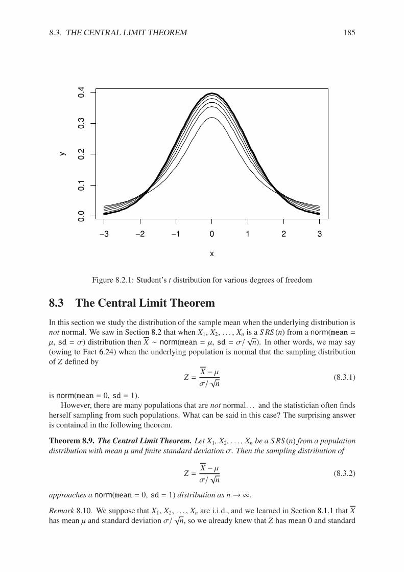
8.3. THE CENTRAL LIMIT THEOREM 185
!3 !2 !1 0 1 2 3
0.0
0.1
0.2
0.3
0.4
x
y
Figure 8.2.1: Student’s t distribution for various degrees of freedom
8.3 The Central Limit Theorem
In this section we study the distribution of the sample mean when the underlying distribution isnot normal. We saw in Section 8.2 that when X1, X2, . . . , Xn is a SRS (n) from a norm(mean =µ, sd = ") distribution then X 4 norm(mean = µ, sd = "/
$n). In other words, we may say
(owing to Fact 6.24) when the underlying population is normal that the sampling distributionof Z defined by
Z =X # µ"/
$n
(8.3.1)
is norm(mean = 0, sd = 1).However, there are many populations that are not normal. . . and the statistician often finds
herself sampling from such populations. What can be said in this case? The surprising answeris contained in the following theorem.
Theorem 8.9. The Central Limit Theorem. Let X1, X2, . . . , Xn be a SRS (n) from a population
distribution with mean µ and finite standard deviation ". Then the sampling distribution of
Z =X # µ"/
$n
(8.3.2)
approaches a norm(mean = 0, sd = 1) distribution as n . &.
Remark 8.10. We suppose that X1, X2, . . . , Xn are i.i.d., and we learned in Section 8.1.1 that Xhas mean µ and standard deviation "/
$n, so we already knew that Z has mean 0 and standard
186 CHAPTER 8. SAMPLING DISTRIBUTIONS
deviation 1. The beauty of the CLT is that it addresses the shape of Z’s distribution when thesample size is large.
Remark 8.11. Notice that the shape of the underlying population’s distribution is not mentionedin Theorem 8.9; indeed, the result is true for any population that is well-behaved enough to havea finite standard deviation. In particular, if the population is normally distributed then we knowfrom Section 8.2.1 that the distribution of X (and Z by extension) is exactly normal, for everyn.
Remark 8.12. How large is “su"ciently large”? It is here that the shape of the underlyingpopulation distribution plays a role. For populations with distributions that are approximatelysymmetric and mound-shaped, the samples may need to be only of size four or five, whilefor highly skewed or heavy-tailed populations the samples may need to be much larger forthe distribution of the sample means to begin to show a bell-shape. Regardless, for a givenpopulation distribution (with finite standard deviation) the approximation tends to be better forlarger sample sizes.
8.3.1 How to do it with R
The TeachingDemos package [79] has clt.examp and the distrTeach [74] package hasillustrateCLT. Try the following at the command line (output omitted):
> library(TeachingDemos)
> example(clt.examp)
and
> library(distrTeach)
> example(illustrateCLT)
The IPSUR package has the functions clt1, clt2, and clt3 (see Exercise 8.2 at the end ofthis chapter). Its purpose is to investigate what happens to the sampling distribution of X whenthe population distribution is mound shaped, finite support, and skewed, namely t(df = 3),unif(a = 0, b = 10) and gamma(shape = 1.21, scale = 1/2.37), respectively.
For example, when the command clt1() is issued a plot window opens to show a graphof the PDF of a t(df = 3) distribution. On the display are shown numerical values of thepopulation mean and variance. While the students examine the graph the computer is simu-lating random samples of size sample.size = 2 from the population = "rt" distributiona total of N.iter = 100000 times, and sample means are calculated of each sample. Nextfollows a histogram of the simulated sample means, which closely approximates the samplingdistribution of X, see Section 8.5. Also show are the sample mean and sample variance of allof the simulated Xs. As a final step, when the student clicks the second plot, a normal curvewith the same mean and variance as the simulated Xs is superimposed over the histogram. Stu-dents should compare the population theoretical mean and variance to the simulated mean andvariance of the sampling distribution. They should also compare the shape of the simulatedsampling distribution to the shape of the normal distribution.
The three separate clt1, clt2, and clt3 functions were written so that students couldcompare what happens overall when the shape of the population distribution changes. It wouldbe possible to combine all three into one big function, clt which covers all three cases (andmore).
8.4. SAMPLING DISTRIBUTIONS OF TWO-SAMPLE STATISTICS 187
8.4 Sampling Distributions of Two-Sample Statistics
There are often two populations under consideration, and it sometimes of interest to compareproperties between groups. To do so we take independent samples from each population andcalculate respective sample statistics for comparison. In some simple cases the sampling distri-bution of the comparison is known and easy to derive; such cases are the subject of the presentsection.
8.4.1 Di!erence of Independent Sample Means
Proposition 8.13. Let X1, X2, . . . , Xn1 be an SRS (n1) from a norm(mean = µX, sd = "X) dis-tribution and let Y1, Y2, . . . , Yn2 be an SRS (n2) from a norm(mean = µY , sd = "Y) distribution.Suppose that X1, X2, . . . , Xn1 and Y1, Y2, . . . , Yn2 are independent samples. Then the quantity
X # Y # (µX # µY)M"2
X
Tn1 + "
2Y
Tn2
(8.4.1)
has a norm(mean = 0, sd = 1) sampling distribution. Equivalently, X # Y has a norm(mean =
µX # µY , sd =M"2
X
Tn1 + "
2Y
Tn2) sampling distribution.
Proof. We know that X is norm(mean = µX, sd = "X/$n1) and we also know that Y is
norm(mean = µY , sd = "Y/$n2). And since the samples X1, X2, . . . , Xn1 and Y1, Y2, . . . , Yn2
are independent, so too are X and Y . The distribution of their di!erence is thus normal as well,and the mean and standard deviation are given by Proposition 7.20. "
Remark 8.14. Even if the distribution of one or both of the samples is not normal, the quantityin Equation 8.4.1 will be approximately normal provided both sample sizes are large.
Remark 8.15. For the special case of µX = µY we have shown that
X # YM"2
X/n1 + "2Y/n2
(8.4.2)
has a norm(mean = 0, sd = 1) sampling distribution, or in other words, X#Y has a norm(mean =
0, sd =M"2
X/n1 + "2Y/n2) sampling distribution. This will be important when it comes time
to do hypothesis tests; see Section 9.3.
8.4.2 Di!erence of Independent Sample Proportions
Proposition 8.16. Let X1, X2, . . . , Xn1 be an SRS (n1) from a binom(size = 1, prob = p1)distribution and let Y1, Y2, . . . , Yn2 be an SRS (n2) from a binom(size = 1, prob = p2)distribution. Suppose that X1, X2, . . . , Xn1 and Y1, Y2, . . . , Yn2 are independent samples. Define
p1 =1
n1
n1!
i=1
Xi and p2 =1
n2
n2!
j=1
Yj. (8.4.3)
Then the sampling distribution of
p1 # p2 # (p1 # p2)Mp1(1#p1)
n1+
p2(1#p2)n2
(8.4.4)
188 CHAPTER 8. SAMPLING DISTRIBUTIONS
approaches a norm(mean = 0, sd = 1) distribution as both n1, n2 . &. In other words, the
sampling distribution of p1 # p2 is approximately
norm
$%%%%&mean = p1 # p2, sd =
Up1(1 # p1)
n1+
p2(1 # p2)
n2
())))* , (8.4.5)
provided both n1 and n2 are su!ciently large.
Proof. We know that p1 is approximately normal for n1 su"ciently large by the CLT, and weknow that p2 is approximately normal for n2 su"ciently large, also by the CLT. Further, p1and p2 are independent since they are derived from independent samples. And a di!erence ofindependent (approximately) normal distributions is (approximately) normal, by Exercise 7.31.The expressions for the mean and standard deviation follow immediately from Proposition 7.20combined with the formulas for the binom(size = 1, prob = p) distribution from Chapter5. "
8.4.3 Ratio of Independent Sample Variances
Proposition 8.18. Let X1, X2, . . . , Xn1 be an SRS (n1) from a norm(mean = µX, sd = "X) dis-tribution and let Y1, Y2, . . . , Yn2 be an SRS (n2) from a norm(mean = µY , sd = "Y) distribution.Suppose that X1, X2, . . . , Xn1 and Y1, Y2, . . . , Yn2 are independent samples. Then the ratio
F ="2
YS2X
"2XS
2Y
(8.4.6)
has an f(df1 = n1 # 1, df2 = n2 # 1) sampling distribution.
Proof. We know from Theorem 8.5 that (n1 # 1)S 2X/"
2X is distributed chisq(df = n1 # 1) and
(n2 # 1)S 2Y/"
2Y is distributed chisq(df = n2 # 1). Now write
F ="2
YS2X
"2XS
2Y
=(n1 # 1)S 2
Y
T(n1 # 1)
(n2 # 1)S 2Y
T(n2 # 1)
·1/"2
X
1/"2Y
,
by multiplying and dividing the numerator with n1 # 1 and doing likewise for the denominatorwith n2 # 1. Now we may regroup the terms into
F =
(n1#1)S 2X
"2X
V(n1 # 1)
(n2#1)S 2Y
"2Y
V(n2 # 1)
,
and we recognize F to be the ratio of independent chisq distributions, each divided by itsrespective numerator df = n1 # 1 and denominator df = n1 # 1 degrees of freedom. This is,indeed, the definition of Snedecor’s F distribution. "
1
Remark 8.17. This does not explicitly follow, because of our cavalier use of “approximately” in too many places.To be more thorough, however, would require more concepts than we can a!ord at the moment. The interestedreader may consult a more advanced text, specifically the topic of weak convergence, that is, convergence indistribution.
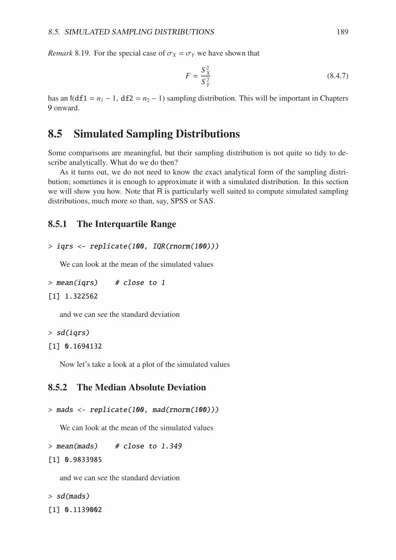
8.5. SIMULATED SAMPLING DISTRIBUTIONS 189
Remark 8.19. For the special case of "X = "Y we have shown that
F =S 2
X
S 2Y
(8.4.7)
has an f(df1 = n1 # 1, df2 = n2 # 1) sampling distribution. This will be important in Chapters9 onward.
8.5 Simulated Sampling Distributions
Some comparisons are meaningful, but their sampling distribution is not quite so tidy to de-scribe analytically. What do we do then?
As it turns out, we do not need to know the exact analytical form of the sampling distri-bution; sometimes it is enough to approximate it with a simulated distribution. In this sectionwe will show you how. Note that R is particularly well suited to compute simulated samplingdistributions, much more so than, say, SPSS or SAS.
8.5.1 The Interquartile Range
> iqrs <- replicate(100, IQR(rnorm(100)))
We can look at the mean of the simulated values
> mean(iqrs) # close to 1
[1] 1.322562
and we can see the standard deviation
> sd(iqrs)
[1] 0.1694132
Now let’s take a look at a plot of the simulated values
8.5.2 The Median Absolute Deviation
> mads <- replicate(100, mad(rnorm(100)))
We can look at the mean of the simulated values
> mean(mads) # close to 1.349
[1] 0.9833985
and we can see the standard deviation
> sd(mads)
[1] 0.1139002
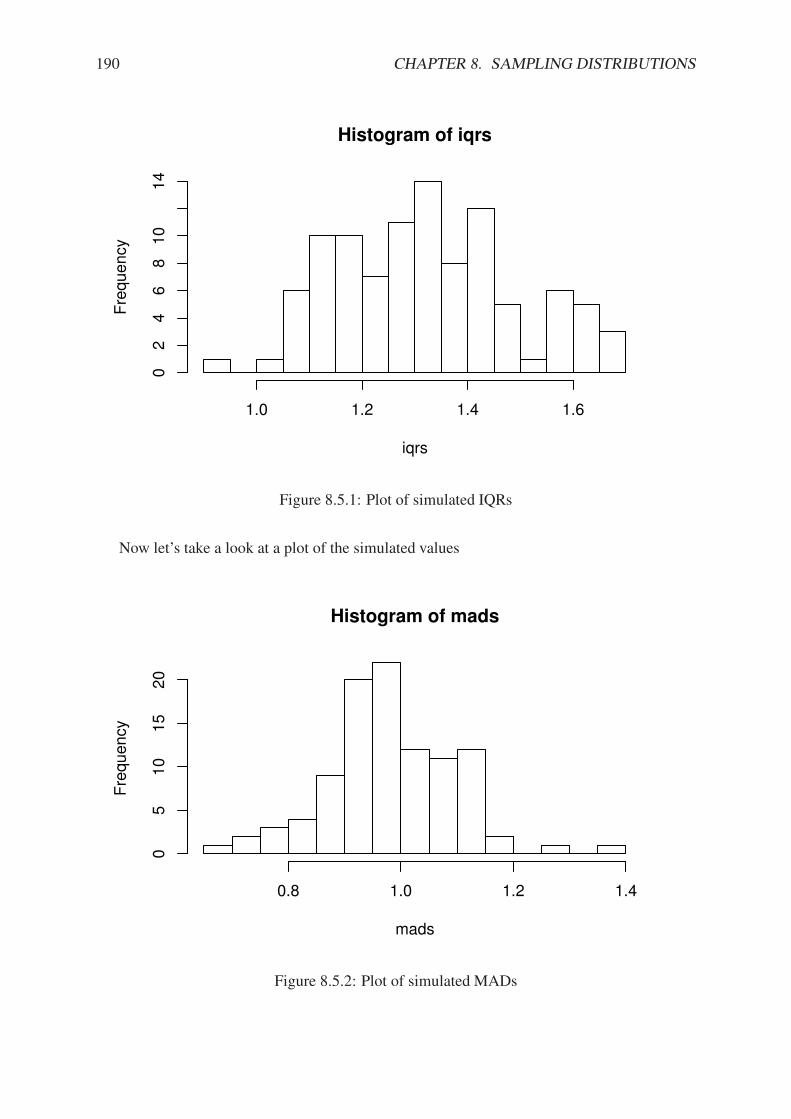
190 CHAPTER 8. SAMPLING DISTRIBUTIONS
Histogram of iqrs
iqrs
Fre
quency
1.0 1.2 1.4 1.6
02
46
810
14
Figure 8.5.1: Plot of simulated IQRs
Now let’s take a look at a plot of the simulated values
Histogram of mads
mads
Fre
quency
0.8 1.0 1.2 1.4
05
10
15
20
Figure 8.5.2: Plot of simulated MADs
8.5. SIMULATED SAMPLING DISTRIBUTIONS 191
Chapter Exercises
Exercise 8.1. Suppose that we observe a random sample X1, X2, . . . , Xn of size SRS (n =19)from a norm(mean =20) distribution.
1. What is the mean of X?
2. What is the standard deviation of X?
3. What is the distribution of X? (approximately)
4. Find IP(a < X " b)
5. Find IP(X > c).
Exercise 8.2. In this exercise we will investigate how the shape of the population distributiona!ects the time until the distribution of X is acceptably normal.
Answer the questions and write a report about what you have learned. Use plots and histogramsto support your conclusions. See Appendix F for instructions about writing reports with R.For these problems, the discussion/interpretation parts are the most important, so be sure toANSWER THE WHOLE QUESTION.
The Central Limit Theorem
For Questions 1-3, we assume that we have observed random variables X1, X2, . . . ,Xn that arean SRS (n) from a given population (depending on the problem) and we want to investigate thedistribution of X as the sample size n increases.
1. The population of interest in this problem has a Student’s t distribution with r = 3 degreesof freedom. We begin our investigation with a sample size of n = 2. Open an R session,make sure to type library(IPSUR) and then follow that with clt1().
(a) Look closely and thoughtfully at the first graph. How would you describe the popu-lation distribution? Think back to the di!erent properties of distributions in Chapter3. Is the graph symmetric? Skewed? Does it have heavy tails or thin tails? Whatelse can you say?
(b) What is the population mean µ and the population variance "2? (Read these fromthe first graph.)
(c) The second graph shows (after a few seconds) a relative frequency histogram whichclosely approximates the distribution of X. Record the values of mean(xbar) andvar(xbar), where xbar denotes the vector that contains the simulated samplemeans. Use the answers from part (b) to calculate what these estimates should
be, based on what you know about the theoretical mean and variance of X. Howwell do your answers to parts (b) and (c) agree?
(d) Click on the histogram to superimpose a red normal curve, which is the theoreticallimit of the distribution of X as n . &. How well do the histogram and the normalcurve match? Describe the di!erences between the two distributions. When judg-ing between the two, do not worry so much about the scale (the graphs are beingrescaled automatically, anyway). Rather, look at the peak: does the histogram poke
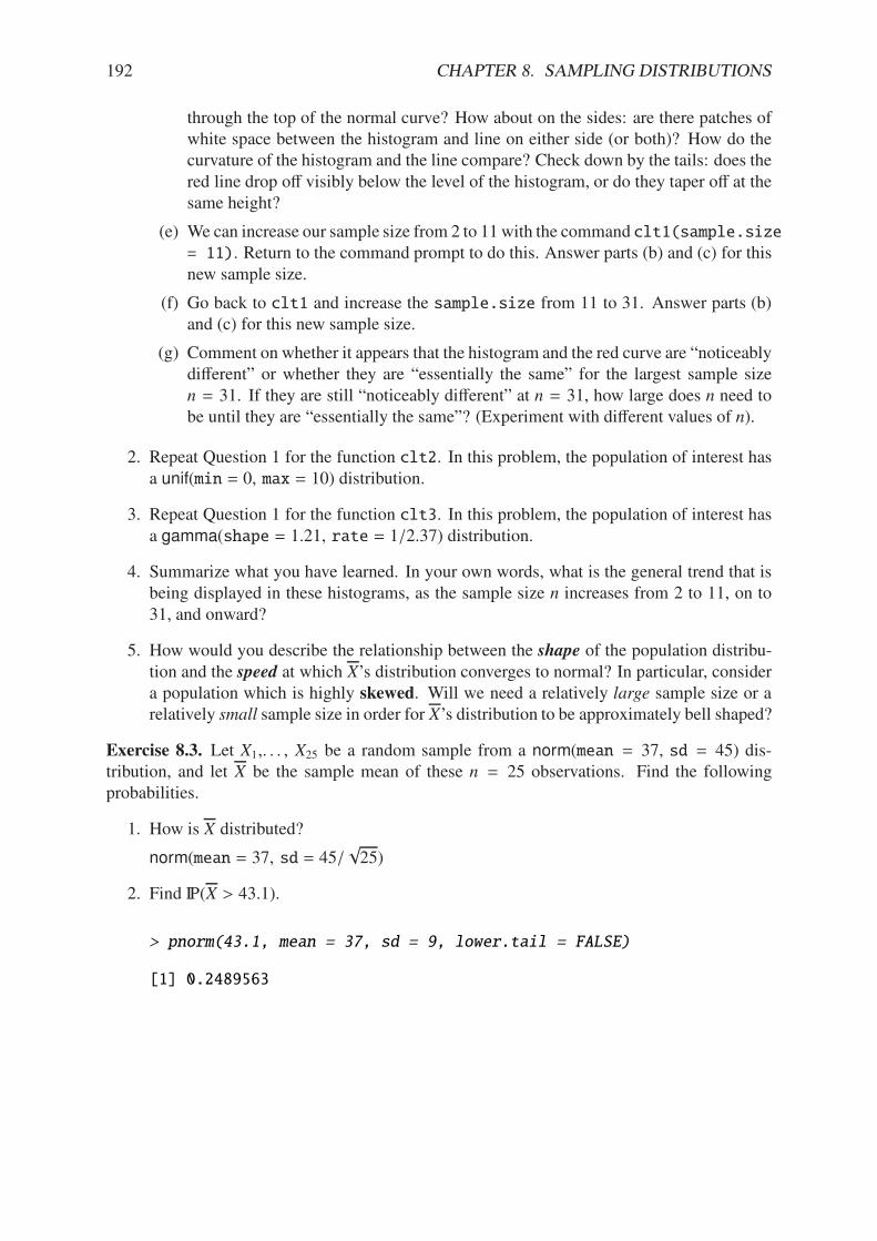
192 CHAPTER 8. SAMPLING DISTRIBUTIONS
through the top of the normal curve? How about on the sides: are there patches ofwhite space between the histogram and line on either side (or both)? How do thecurvature of the histogram and the line compare? Check down by the tails: does thered line drop o! visibly below the level of the histogram, or do they taper o! at thesame height?
(e) We can increase our sample size from 2 to 11 with the command clt1(sample.size= 11). Return to the command prompt to do this. Answer parts (b) and (c) for thisnew sample size.
(f) Go back to clt1 and increase the sample.size from 11 to 31. Answer parts (b)and (c) for this new sample size.
(g) Comment on whether it appears that the histogram and the red curve are “noticeablydi!erent” or whether they are “essentially the same” for the largest sample sizen = 31. If they are still “noticeably di!erent” at n = 31, how large does n need tobe until they are “essentially the same”? (Experiment with di!erent values of n).
2. Repeat Question 1 for the function clt2. In this problem, the population of interest hasa unif(min = 0, max = 10) distribution.
3. Repeat Question 1 for the function clt3. In this problem, the population of interest hasa gamma(shape = 1.21, rate = 1/2.37) distribution.
4. Summarize what you have learned. In your own words, what is the general trend that isbeing displayed in these histograms, as the sample size n increases from 2 to 11, on to31, and onward?
5. How would you describe the relationship between the shape of the population distribu-tion and the speed at which X’s distribution converges to normal? In particular, considera population which is highly skewed. Will we need a relatively large sample size or arelatively small sample size in order for X’s distribution to be approximately bell shaped?
Exercise 8.3. Let X1,. . . , X25 be a random sample from a norm(mean = 37, sd = 45) dis-tribution, and let X be the sample mean of these n = 25 observations. Find the followingprobabilities.
1. How is X distributed?
norm(mean = 37, sd = 45/$25)
2. Find IP(X > 43.1).
> pnorm(43.1, mean = 37, sd = 9, lower.tail = FALSE)
[1] 0.2489563

Chapter 9
Estimation
We will discuss two branches of estimation procedures: point estimation and interval estima-tion. We briefly discuss point estimation first and then spend the rest of the chapter on intervalestimation.
We find an estimator with the methods of Section 9.1. Wemake some assumptions about theunderlying population distribution and use what we know from Chapter 8 about sampling dis-tributions both to study how the estimator will perform, and to find intervals of confidence forunderlying parameters associated with the population distribution. Once we have confidenceintervals we can do inference in the form of hypothesis tests in the next chapter.
What do I want them to know?
• how to look at a problem, identify a reasonable model, and estimate a parameter associ-ated with the model
• about maximum likelihood, and in particular, how to
* eyeball a likelihood to get a maximum
* use calculus to find an MLE for one-parameter families
• about properties of the estimators they find, such as bias, minimum variance, MSE
• point versus interval estimation, and how to find and interpret confidence intervals forbasic experimental designs
• the concept of margin of error and its relationship to sample size
9.1 Point Estimation
The following example is how I was introduced to maximum likelihood.
Example 9.1. Suppose we have a small pond in our backyard, and in the pond there live somefish. We would like to know how many fish live in the pond. How can we estimate this? Oneprocedure developed by researchers is the capture-recapture method. Here is how it works.
We will fish from the pond and suppose that we capture M = 7 fish. On each caught fishwe attach an unobtrusive tag to the fish’s tail, and release it back into the water.
193
194 CHAPTER 9. ESTIMATION
Next, we wait a few days for the fish to remix and become accustomed to their new tag.Then we go fishing again. On the second trip some of the fish we catch may be tagged; somemay not be. Let X denote the number of caught fish which are tagged1, and suppose for thesake of argument that we catch K = 4 fish and we find that 3 of them are tagged.
Now let F denote the (unknown) total number of fish in the pond. We know that F / 7,because we tagged that many on the first trip. In fact, if we let N denote the number of untaggedfish in the pond, then F = M + N. We have sampled K = 4 times, without replacement, froman urn which has M = 7 white balls and N = F # M black balls, and we have observed x = 3of them to be white. What is the probability of this?
Looking back to Section 5.6, we see that the random variable X has a hyper(m = M, n =
F # M, k = K) distribution. Therefore, for an observed value X = x the probability would be
IP(X = x) =
2Mx
32F#MK#x
3
2FK
3 .
First we notice that F must be at least 7. Could F be equal to seven? If F = 7 then all of thefish would have been tagged on the first run, and there would be no untagged fish in the pond,thus, IP(3 successes in 4 trials) = 0.
What about F = 8; what would be the probability of observing X = 3 tagged fish?
IP(3 successes in 4 trials) =
273
3211
3
284
3 =35
70= 0.5.
Similarly, if F = 9 then the probability of observing X = 3 tagged fish would be
IP(3 successes in 4 trials) =
273
3221
3
294
3 =70
126' 0.556.
We can see already that the observed data X = 3 is more likely when F = 9 than it is whenF = 8. And here lies the genius of Sir Ronald Aylmer Fisher: he asks, “What is the value of Fwhich has the highest likelihood?” In other words, for all of the di!erent possible values of F,which one makes the above probability the biggest? We can answer this question with a plot ofIP(X = x) versus F. See Figure 9.1.1.
Example 9.2. In the last example we were only concerned with how many fish were in thepond, but now, we will ask a di!erent question. Suppose it is known that there are only twospecies of fish in the pond: smallmouth bass (Micropterus dolomieu) and bluegill (Lepomismacrochirus); perhaps we built the pond some years ago and stocked it with only these twospecies. We would like to estimate the proportion of fish in the pond which are bass.
Let p = the proportion of bass. Without any other information, it is conceivable for p to beany value in the interval [0, 1], but for the sake of argument we will suppose that p falls strictlybetween 0 and 1. How can we learn about the true value of p? Go fishing! As before, wewill use catch-and-release, but unlike before, we will not tag the fish. We will simply note thespecies of any caught fish before returning it to the pond.
1It is theoretically possible that we could catch the same tagged fish more than once, which would inflate ourcount of tagged fish. To avoid this di"culty, suppose that on the second trip we use a tank on the boat to hold thecaught fish until data collection is completed.
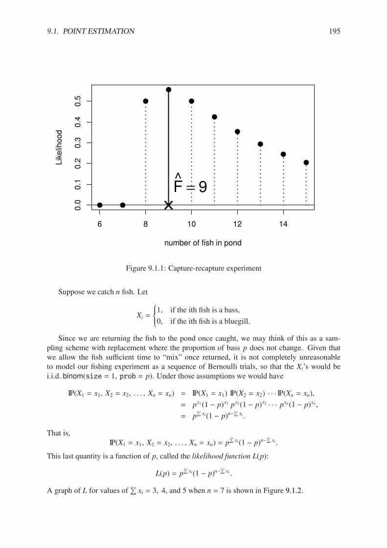
9.1. POINT ESTIMATION 195
6 8 10 12 14
0.0
0.1
0.2
0.3
0.4
0.5
number of fish in pond
Lik
elih
ood
F^
= 9
Figure 9.1.1: Capture-recapture experiment
Suppose we catch n fish. Let
Xi =
9::;::<1, if the ith fish is a bass,
0, if the ith fish is a bluegill.
Since we are returning the fish to the pond once caught, we may think of this as a sam-pling scheme with replacement where the proportion of bass p does not change. Given thatwe allow the fish su"cient time to “mix” once returned, it is not completely unreasonableto model our fishing experiment as a sequence of Bernoulli trials, so that the Xi’s would bei.i.d. binom(size = 1, prob = p). Under those assumptions we would have
IP(X1 = x1, X2 = x2, . . . , Xn = xn) = IP(X1 = x1) IP(X2 = x2) · · · IP(Xn = xn),
= px1 (1 # p)x1 px2 (1 # p)x2 · · · pxn(1 # p)xn ,
= p#
xi(1 # p)n##
xi .
That is,IP(X1 = x1, X2 = x2, . . . , Xn = xn) = p
#xi(1 # p)n#
#xi .
This last quantity is a function of p, called the likelihood function L(p):
L(p) = p#
xi(1 # p)n##
xi .
A graph of L for values of#
xi = 3, 4, and 5 when n = 7 is shown in Figure 9.1.2.
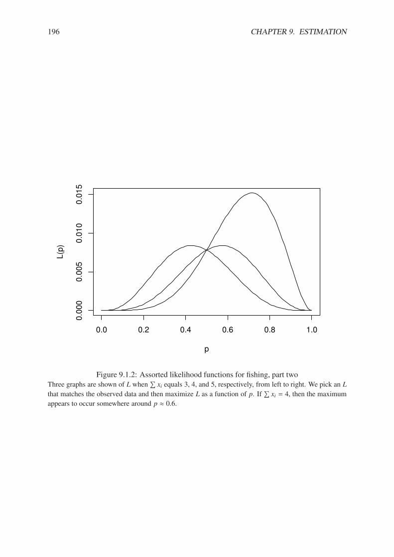
196 CHAPTER 9. ESTIMATION
0.0 0.2 0.4 0.6 0.8 1.0
0.0
00
0.0
05
0.0
10
0.0
15
p
L(p
)
Figure 9.1.2: Assorted likelihood functions for fishing, part twoThree graphs are shown of L when
#xi equals 3, 4, and 5, respectively, from left to right. We pick an L
that matches the observed data and then maximize L as a function of p. If#
xi = 4, then the maximum
appears to occur somewhere around p ' 0.6.
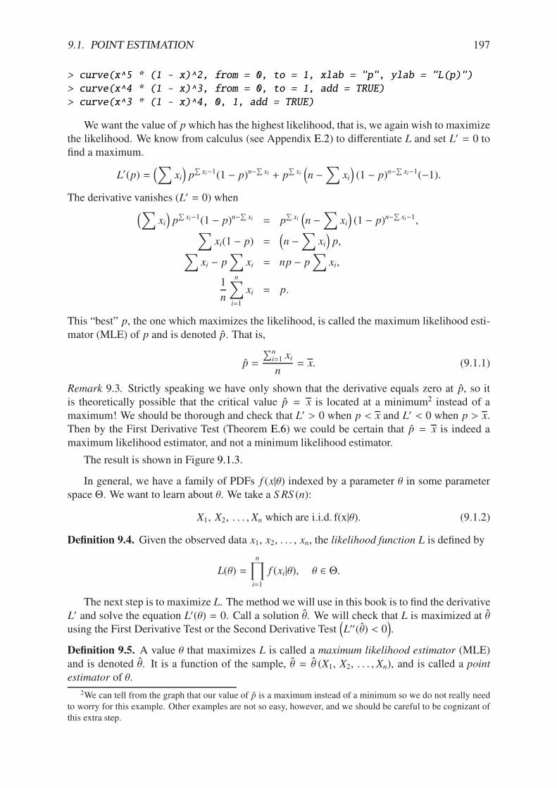
9.1. POINT ESTIMATION 197
> curve(x^5 * (1 - x)^2, from = 0, to = 1, xlab = "p", ylab = "L(p)")
> curve(x^4 * (1 - x)^3, from = 0, to = 1, add = TRUE)
> curve(x^3 * (1 - x)^4, 0, 1, add = TRUE)
We want the value of p which has the highest likelihood, that is, we again wish to maximizethe likelihood. We know from calculus (see Appendix E.2) to di!erentiate L and set L5 = 0 tofind a maximum.
L5(p) =2!
xi3p
#xi#1(1 # p)n#
#xi + p
#xi
2n #
!xi
3(1 # p)n#
#xi#1(#1).
The derivative vanishes (L5 = 0) when2!
xi3p
#xi#1(1 # p)n#
#xi = p
#xi
2n #
!xi
3(1 # p)n#
#xi#1,
!xi(1 # p) =
2n #
!xi
3p,
!xi # p
!xi = np # p
!xi,
1
n
n!
i=1
xi = p.
This “best” p, the one which maximizes the likelihood, is called the maximum likelihood esti-mator (MLE) of p and is denoted p. That is,
p =
#ni=1 xi
n= x. (9.1.1)
Remark 9.3. Strictly speaking we have only shown that the derivative equals zero at p, so itis theoretically possible that the critical value p = x is located at a minimum2 instead of amaximum! We should be thorough and check that L5 > 0 when p < x and L5 < 0 when p > x.Then by the First Derivative Test (Theorem E.6) we could be certain that p = x is indeed amaximum likelihood estimator, and not a minimum likelihood estimator.
The result is shown in Figure 9.1.3.
In general, we have a family of PDFs f (x|,) indexed by a parameter , in some parameterspace '. We want to learn about ,. We take a SRS (n):
X1, X2, . . . , Xn which are i.i.d. f(x|,). (9.1.2)
Definition 9.4. Given the observed data x1, x2, . . . , xn, the likelihood function L is defined by
L(,) =nW
i=1
f (xi|,), , 3 '.
The next step is to maximize L. The method we will use in this book is to find the derivativeL5 and solve the equation L5(,) = 0. Call a solution ,. We will check that L is maximized at ,using the First Derivative Test or the Second Derivative Test
2L55(,) < 0
3.
Definition 9.5. A value , that maximizes L is called a maximum likelihood estimator (MLE)and is denoted ,. It is a function of the sample, , = , (X1, X2, . . . , Xn), and is called a point
estimator of ,.2We can tell from the graph that our value of p is a maximum instead of a minimum so we do not really need
to worry for this example. Other examples are not so easy, however, and we should be careful to be cognizant ofthis extra step.
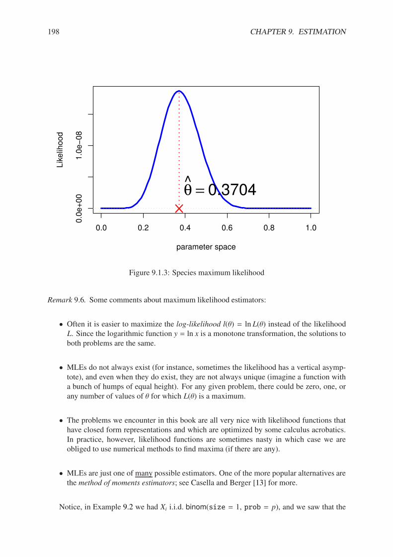
198 CHAPTER 9. ESTIMATION
0.0 0.2 0.4 0.6 0.8 1.0
0.0
e+
00
1.0
e!
08
parameter space
Lik
elih
ood
! = 0.3704
Figure 9.1.3: Species maximum likelihood
Remark 9.6. Some comments about maximum likelihood estimators:
• Often it is easier to maximize the log-likelihood l(,) = ln L(,) instead of the likelihoodL. Since the logarithmic function y = ln x is a monotone transformation, the solutions toboth problems are the same.
• MLEs do not always exist (for instance, sometimes the likelihood has a vertical asymp-tote), and even when they do exist, they are not always unique (imagine a function witha bunch of humps of equal height). For any given problem, there could be zero, one, orany number of values of , for which L(,) is a maximum.
• The problems we encounter in this book are all very nice with likelihood functions thathave closed form representations and which are optimized by some calculus acrobatics.In practice, however, likelihood functions are sometimes nasty in which case we areobliged to use numerical methods to find maxima (if there are any).
• MLEs are just one of many possible estimators. One of the more popular alternatives arethe method of moments estimators; see Casella and Berger [13] for more.
Notice, in Example 9.2 we had Xi i.i.d. binom(size = 1, prob = p), and we saw that the
9.1. POINT ESTIMATION 199
MLE was p = X. But further
IE X = IEX1 + X2 + · · · + Xn
n,
=1
n(IE X1 + IE X2 + · · · + IE Xn) ,
=1
n(np) ,
= p,
which is exactly the same as the parameter which we estimated. More concisely, IE p = p, thatis, on the average, the estimator is exactly right.
Definition 9.7. Let s(X1, X2, . . . , Xn) be a statistic which estimates ,. If
IE s(X1, X2, . . . , Xn) = ,,
then the statistic s(X1, X2, . . . , Xn) is said to be an unbiased estimator of ,. Otherwise, it isbiased.
Example 9.8. Let X1, X2, . . . , Xn be an SRS (n) from a norm(mean = µ, sd = ") distribution.It can be shown (in Exercise 9.1) that if , = (µ,"2) then the MLE of , is
, = (µ, "2), (9.1.3)
where µ = X and
"2 =1
n
n!
i=1
2Xi # X
32=
n # 1
nS 2. (9.1.4)
We of course know from 8.2 that µ is unbiased. What about "2? Let us check:
IE "2 = IEn # 1
nS 2
= IE
0"2
n
(n # 1)S 2
"2
1
="2
nIE chisq(df = n # 1)
="2
n(n # 1),
from which we may conclude two things:
1. "2 is a biased estimator of "2, and
2. S 2 = n"2/(n # 1) is an unbiased estimator of "2.
One of the most common questions in an introductory statistics class is, “Why do we divideby n # 1 when we compute the sample variance? Why do we not divide by n?” We see nowthat division by n amounts to the use of a biased estimator for "2, that is, if we divided by n
then on the average we would underestimate the true value of "2. We use n # 1 so that, on theaverage, our estimator of "2 will be exactly right.
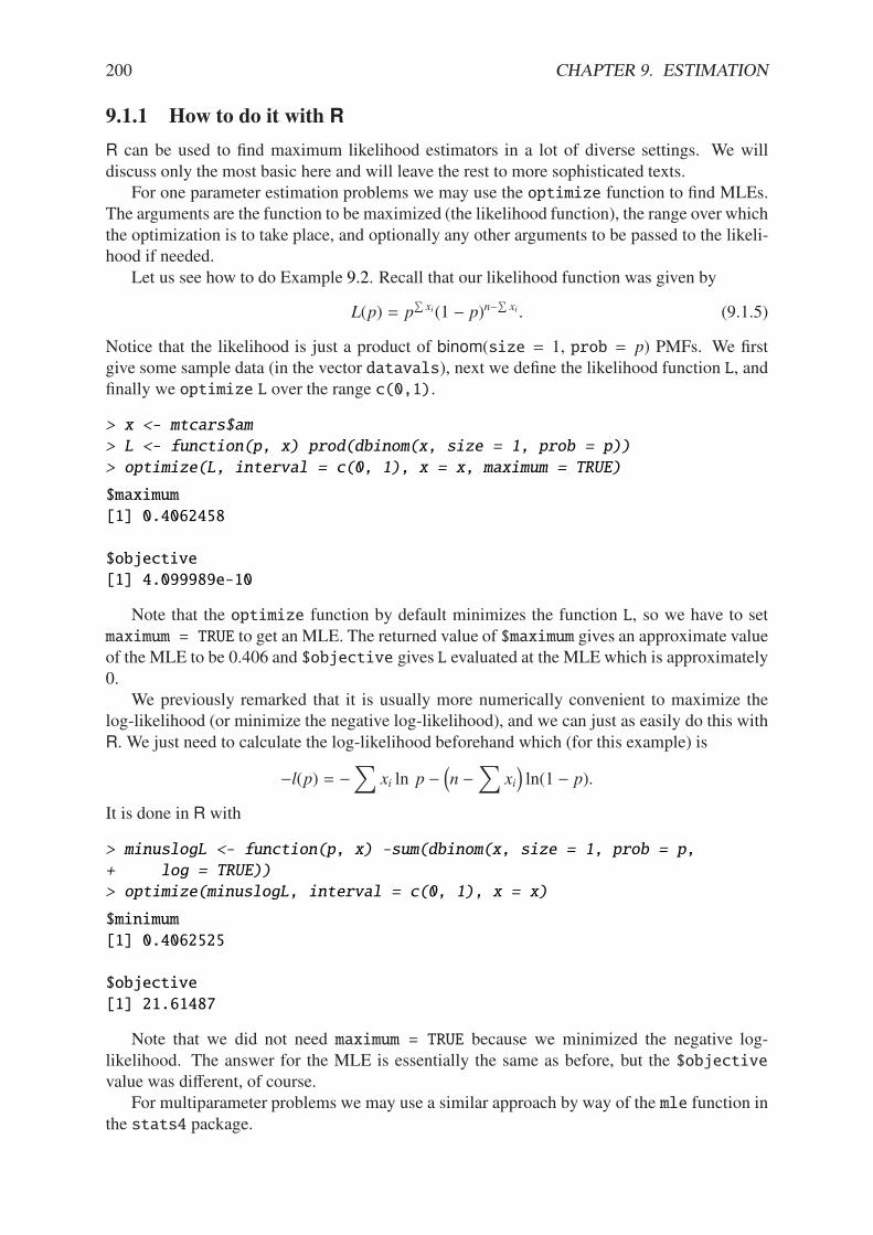
200 CHAPTER 9. ESTIMATION
9.1.1 How to do it with R
R can be used to find maximum likelihood estimators in a lot of diverse settings. We willdiscuss only the most basic here and will leave the rest to more sophisticated texts.
For one parameter estimation problems we may use the optimize function to find MLEs.The arguments are the function to be maximized (the likelihood function), the range over whichthe optimization is to take place, and optionally any other arguments to be passed to the likeli-hood if needed.
Let us see how to do Example 9.2. Recall that our likelihood function was given by
L(p) = p#
xi(1 # p)n##
xi . (9.1.5)
Notice that the likelihood is just a product of binom(size = 1, prob = p) PMFs. We firstgive some sample data (in the vector datavals), next we define the likelihood function L, andfinally we optimize L over the range c(0,1).
> x <- mtcars$am
> L <- function(p, x) prod(dbinom(x, size = 1, prob = p))
> optimize(L, interval = c(0, 1), x = x, maximum = TRUE)
$maximum
[1] 0.4062458
$objective
[1] 4.099989e-10
Note that the optimize function by default minimizes the function L, so we have to setmaximum = TRUE to get an MLE. The returned value of $maximum gives an approximate valueof the MLE to be 0.406 and $objective gives L evaluated at the MLE which is approximately0.
We previously remarked that it is usually more numerically convenient to maximize thelog-likelihood (or minimize the negative log-likelihood), and we can just as easily do this withR. We just need to calculate the log-likelihood beforehand which (for this example) is
#l(p) = #!
xi ln p #2n #
!xi
3ln(1 # p).
It is done in R with
> minuslogL <- function(p, x) -sum(dbinom(x, size = 1, prob = p,
+ log = TRUE))
> optimize(minuslogL, interval = c(0, 1), x = x)
$minimum
[1] 0.4062525
$objective
[1] 21.61487
Note that we did not need maximum = TRUE because we minimized the negative log-likelihood. The answer for the MLE is essentially the same as before, but the $objectivevalue was di!erent, of course.
For multiparameter problems we may use a similar approach by way of the mle function inthe stats4 package.
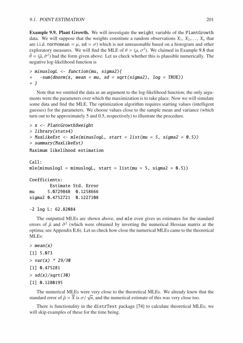
9.1. POINT ESTIMATION 201
Example 9.9. Plant Growth. We will investigate the weight variable of the PlantGrowthdata. We will suppose that the weights constitute a random observations X1, X2,. . . , Xn thatare i.i.d. norm(mean = µ, sd = ") which is not unreasonable based on a histogram and otherexploratory measures. We will find the MLE of , = (µ,"2). We claimed in Example 9.8 that, = (µ, "2) had the form given above. Let us check whether this is plausible numerically. Thenegative log-likelihood function is
> minuslogL <- function(mu, sigma2){
+ -sum(dnorm(x, mean = mu, sd = sqrt(sigma2), log = TRUE))
+ }
Note that we omitted the data as an argument to the log-likelihood function; the only argu-ments were the parameters over which the maximization is to take place. Now we will simulatesome data and find the MLE. The optimization algorithm requires starting values (intelligentguesses) for the parameters. We choose values close to the sample mean and variance (whichturn out to be approximately 5 and 0.5, respectively) to illustrate the procedure.
> x <- PlantGrowth$weight
> library(stats4)
> MaxLikeEst <- mle(minuslogL, start = list(mu = 5, sigma2 = 0.5))
> summary(MaxLikeEst)
Maximum likelihood estimation
Call:
mle(minuslogl = minuslogL, start = list(mu = 5, sigma2 = 0.5))
Coefficients:
Estimate Std. Error
mu 5.0729848 0.1258666
sigma2 0.4752721 0.1227108
-2 log L: 62.82084
The outputted MLEs are shown above, and mle even gives us estimates for the standarderrors of µ and "2 (which were obtained by inverting the numerical Hessian matrix at theoptima; see Appendix E.6). Let us check how close the numerical MLEs came to the theoreticalMLEs:
> mean(x)
[1] 5.073
> var(x) * 29/30
[1] 0.475281
> sd(x)/sqrt(30)
[1] 0.1280195
The numerical MLEs were very close to the theoretical MLEs. We already knew that thestandard error of µ = X is "/
$n, and the numerical estimate of this was very close too.
There is functionality in the distrTest package [74] to calculate theoretical MLEs; wewill skip examples of these for the time being.
202 CHAPTER 9. ESTIMATION
9.2 Confidence Intervals for Means
We are given X1, X2, . . . , Xn that are an SRS (n) from a norm(mean = µ, sd = ") distribution,where µ is unknown. We know that we may estimate µ with X, and we have seen that thisestimator is the MLE. But how good is our estimate? We know that
X # µ"/
$n4 norm(mean = 0, sd = 1). (9.2.1)
For a big probability 1 # (, for instance, 95%, we can calculate the quantile z(/2. Then
IP
$%%%%&#z(/2 "
X # µ"/
$n" z(/2
())))* = 1 # (. (9.2.2)
But now consider the following string of equivalent inequalities:
#z(/2 "X # µ"/
$n" z(/2,
#z(/2
0"$n
1" X # µ " z(/2
0"$n
1,
#X # z(/2
0"$n
1" #µ " #X + z(/2
0"$n
1,
X # z(/2
0"$n
1" µ " X + z(/2
0"$n
1.
That is,
IP
0X # z(/2
"$n" µ " X + z(/2
"$n
1= 1 # (. (9.2.3)
Definition 9.10. The interval7X # z(/2
"$n, X + z(/2
"$n
8(9.2.4)
is a 100(1#()% confidence interval for µ. The quantity 1#( is called the confidence coe!cient.
Remark 9.11. The interval is also sometimes written more compactly as
X ± z(/2"$n. (9.2.5)
The interpretation of confidence intervals is tricky and often mistaken by novices. When Iam teaching the concept “live” during class, I usually ask the students to imagine that my pieceof chalk represents the “unknown” parameter, and I lay it down on the desk in front of me.Once the chalk has been lain, it is fixed; it does not move. Our goal is to estimate the parameter.For the estimator I pick up a sheet of loose paper lying nearby. The estimation procedure is torandomly drop the piece of paper from above, and observe where it lands. If the piece of papercovers the piece of chalk, then we are successful – our estimator covers the parameter. If it fallso! to one side or the other, then we are unsuccessful; our interval fails to cover the parameter.
9.2. CONFIDENCE INTERVALS FOR MEANS 203
Then I ask them: suppose we were to repeat this procedure hundreds, thousands, millionsof times. Suppose we kept track of how many times we covered and how many times we didnot. What percentage of the time would we be successful?
In the demonstration, the parameter corresponds to the chalk, the sheet of paper correspondsto the confidence interval, and the random experiment corresponds to dropping the sheet ofpaper. The percentage of the time that we are successful exactly corresponds to the confidencecoe!cient. That is, if we use a 95% confidence interval, then we can say that, in the long run,approximately 95% of our intervals will cover the true parameter (which is fixed, but unknown).
See Figure 9.2.1, which is a graphical display of these ideas.Under the above framework, we can reason that an “interval” with a larger confidence
coe"cient corresponds to a wider sheet of paper. Furthermore, the width of the confidenceinterval (sheet of paper) should be somehow related to the amount of information contained inthe random sample, X1, X2, . . . , Xn. The following remarks makes these notions precise.
Remark 9.12. For a fixed confidence coe"cient 1 # (,
if n increases, then the confidence interval gets SHORTER. (9.2.6)
Remark 9.13. For a fixed sample size n,
if 1 # ( increases, then the confidence interval getsWIDER. (9.2.7)
Example 9.14. Results from an Experiment on Plant Growth. The PlantGrowth dataframe gives the results of an experiment to measure plant yield (as measured by the weightof the plant). We would like to a 95% confidence interval for the mean weight of the plants.Suppose that we know from prior research that the true population standard deviation of theplant weights is 0.7 g.
The parameter of interest is µ, which represents the true mean weight of the population ofall plants of the particular species in the study. We will first take a look at a stemplot of thedata:
> library(aplpack)
> with(PlantGrowth, stem.leaf(weight))
1 | 2: represents 1.2
leaf unit: 0.1
n: 30
1 f | 5
s |
2 3. | 8
4 4* | 11
5 t | 3
8 f | 455
10 s | 66
13 4. | 889
(4) 5* | 1111
13 t | 2233
9 f | 555
s |
6 5. | 88
4 6* | 011
1 t | 3
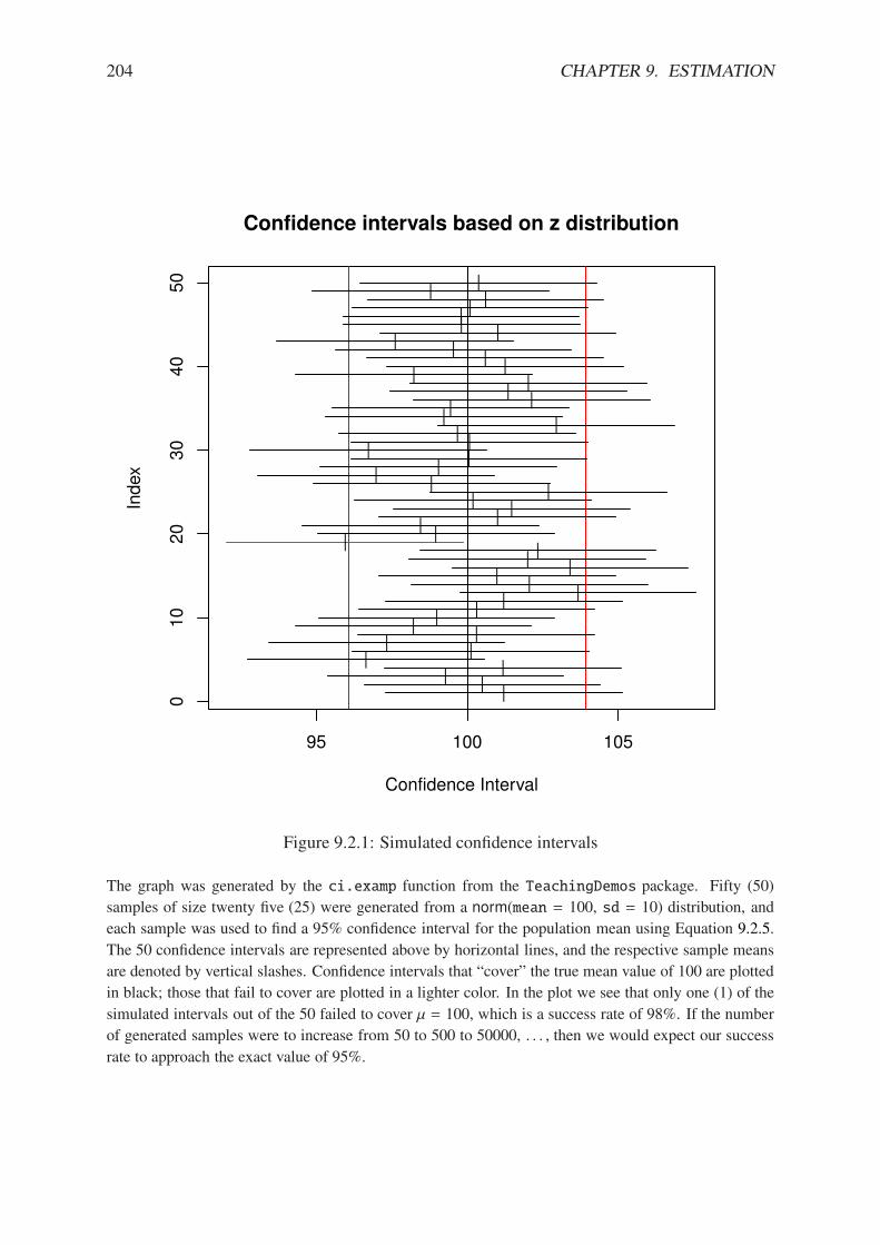
204 CHAPTER 9. ESTIMATION
95 100 105
010
20
30
40
50
Confidence Interval
Ind
ex
Confidence intervals based on z distribution
||| || || || | | | ||| || || || | || ||| | || || || ||| || |||| |||
| || |
Figure 9.2.1: Simulated confidence intervals
The graph was generated by the ci.examp function from the TeachingDemos package. Fifty (50)
samples of size twenty five (25) were generated from a norm(mean = 100, sd = 10) distribution, and
each sample was used to find a 95% confidence interval for the population mean using Equation 9.2.5.
The 50 confidence intervals are represented above by horizontal lines, and the respective sample means
are denoted by vertical slashes. Confidence intervals that “cover” the true mean value of 100 are plotted
in black; those that fail to cover are plotted in a lighter color. In the plot we see that only one (1) of the
simulated intervals out of the 50 failed to cover µ = 100, which is a success rate of 98%. If the number
of generated samples were to increase from 50 to 500 to 50000, . . . , then we would expect our success
rate to approach the exact value of 95%.
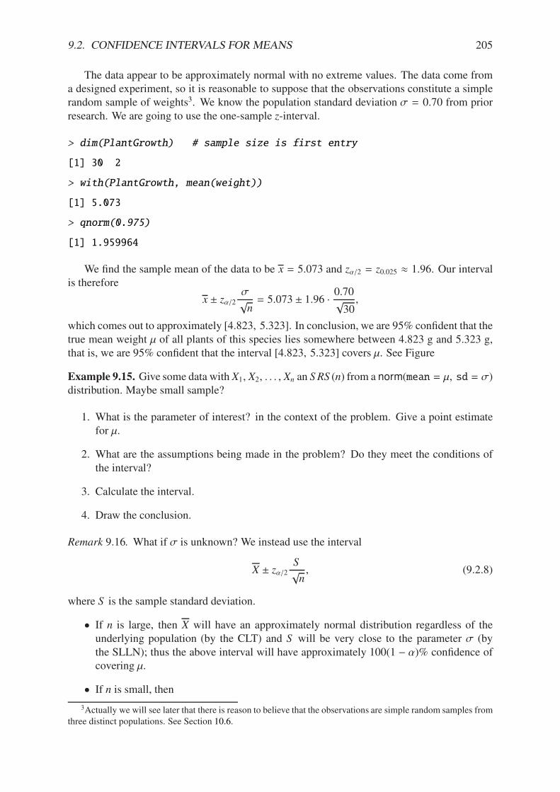
9.2. CONFIDENCE INTERVALS FOR MEANS 205
The data appear to be approximately normal with no extreme values. The data come froma designed experiment, so it is reasonable to suppose that the observations constitute a simplerandom sample of weights3. We know the population standard deviation " = 0.70 from priorresearch. We are going to use the one-sample z-interval.
> dim(PlantGrowth) # sample size is first entry
[1] 30 2
> with(PlantGrowth, mean(weight))
[1] 5.073
> qnorm(0.975)
[1] 1.959964
We find the sample mean of the data to be x = 5.073 and z(/2 = z0.025 ' 1.96. Our intervalis therefore
x ± z(/2"$n= 5.073 ± 1.96 ·
0.70$30,
which comes out to approximately [4.823, 5.323]. In conclusion, we are 95% confident that thetrue mean weight µ of all plants of this species lies somewhere between 4.823 g and 5.323 g,that is, we are 95% confident that the interval [4.823, 5.323] covers µ. See Figure
Example 9.15. Give some data with X1, X2, . . . , Xn an SRS (n) from a norm(mean = µ, sd = ")distribution. Maybe small sample?
1. What is the parameter of interest? in the context of the problem. Give a point estimatefor µ.
2. What are the assumptions being made in the problem? Do they meet the conditions ofthe interval?
3. Calculate the interval.
4. Draw the conclusion.
Remark 9.16. What if " is unknown? We instead use the interval
X ± z(/2S$n, (9.2.8)
where S is the sample standard deviation.
• If n is large, then X will have an approximately normal distribution regardless of theunderlying population (by the CLT) and S will be very close to the parameter " (bythe SLLN); thus the above interval will have approximately 100(1 # ()% confidence ofcovering µ.
• If n is small, then
3Actually we will see later that there is reason to believe that the observations are simple random samples fromthree distinct populations. See Section 10.6.
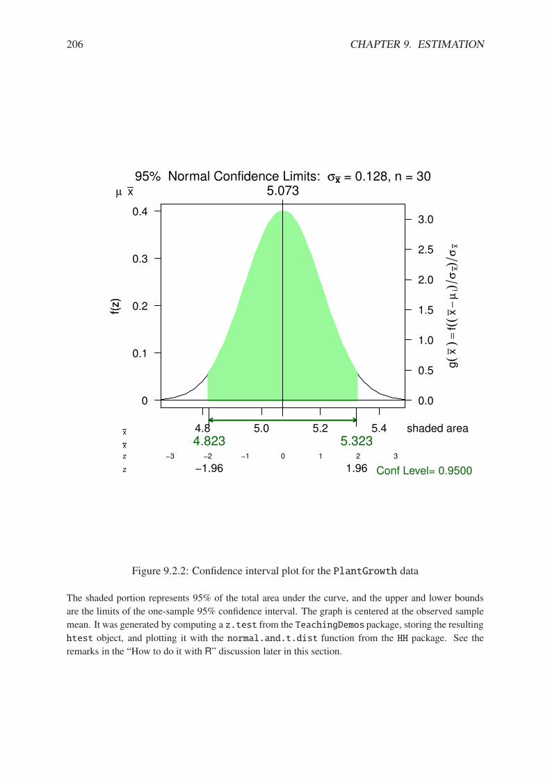
206 CHAPTER 9. ESTIMATION
4.8 5.0 5.2 5.4
95% Normal Confidence Limits: "x = 0.128, n = 30
f(z)
0.0
0.5
1.0
1.5
2.0
2.5
3.0
!3 !2 !1 0 1 2 3
0
0.1
0.2
0.3
0.4
g(
x )
=f(
( x#
µ i)
" x)"
x
f(z)
!1.96 1.96z
z
shaded area
Conf Level= 0.9500
4.823 5.323x
x
µ x 5.073
Figure 9.2.2: Confidence interval plot for the PlantGrowth data
The shaded portion represents 95% of the total area under the curve, and the upper and lower bounds
are the limits of the one-sample 95% confidence interval. The graph is centered at the observed sample
mean. It was generated by computing a z.test from the TeachingDemos package, storing the resulting
htest object, and plotting it with the normal.and.t.dist function from the HH package. See the
remarks in the “How to do it with R” discussion later in this section.
9.2. CONFIDENCE INTERVALS FOR MEANS 207
* If the underlying population is normal then we may replace z(/2 with t(/2(df =n # 1). The resulting 100(1 # ()% confidence interval is
X ± t(/2(df = n # 1)S$n
(9.2.9)
* if the underlying population is not normal, but approximately normal, then we mayuse the t interval, Equation 9.2.9. The interval will have approximately 100(1#()%confidence of covering µ. However, if the population is highly skewed or the datahave outliers, then we should ask a professional statistician for advice.
The author learned of a handy acronym from AP Statistics Exam graders that summarizes theimportant parts of confidence interval estimation, which is PANIC: Parameter, Assumptions,Name, Interval, and Conclusion.
Parameter: identify the parameter of interest with the proper symbols. Write down what theparameter means in the context of the problem.
Assumptions: list any assumptions made in the experiment. If there are any other assumptionsneeded or that were not checked, state what they are and why they are important.
Name: choose a statistical procedure from your bag of tricks based on the answers to theprevious two parts. The assumptions of the procedure you choose should match those ofthe problem; if they do not match then either pick a di!erent procedure or openly admitthat the results may not be reliable. Write down any underlying formulas used.
Interval: calculate the interval from the sample data. This can be done by hand but will moreoften be done with the aid of a computer. Regardless of the method, all calculations orcode should be shown so that the entire process is repeatable by a subsequent reader.
Conclusion: state the final results, using language in the context of the problem. Include theappropriate interpretation of the interval, making reference to the confidence coe"cient.
Remark 9.17. All of the above intervals for µ were two-sided, but there are also one-sidedintervals for µ. They look like
7X # z(
"$n, &
1or
0#&, X + z(
"$n
8(9.2.10)
and satisfy
IP
0X # z(
"$n" µ
1= 1 # ( and IP
0X + z(
"$n/ µ
1= 1 # (. (9.2.11)
Example 9.18. Small sample, some data with X1, X2, . . . , Xn an SRS (n) from a norm(mean =µ, sd = ") distribution.
1. PANIC

208 CHAPTER 9. ESTIMATION
9.2.1 How to do it with R
We can do Example 9.14 with the following code.
> library(TeachingDemos)
> temp <- with(PlantGrowth, z.test(weight, stdev = 0.7))
> temp
One Sample z-test
data: weight
z = 39.6942, n = 30.000, Std. Dev. = 0.700, Std. Dev. of the
sample mean = 0.128, p-value < 2.2e-16
alternative hypothesis: true mean is not equal to 0
95 percent confidence interval:
4.822513 5.323487
sample estimates:
mean of weight
5.073
The confidence interval bounds are shown in the sixth line down of the output (pleasedisregard all of the additional output information for now – we will use it in Chapter 10). Wecan make the plot for Figure 9.2.2 with
> library(IPSUR)
> plot(temp, "Conf")
9.3 Confidence Intervals for Di!erences of Means
Let X1, X2, . . . , Xn be a SRS (n) from a norm(mean = µX, sd = "X) distribution and let Y1, Y2,. . . , Ym be a SRS (m) from a norm(mean = µY , sd = "Y) distribution. Further, assume that theX1, X2, . . . , Xn sample is independent of the Y1, Y2, . . . , Ym sample.
Suppose that "X and "Y are known. We would like a confidence interval for µX # µY . Weknow that
X # Y 4 norm
$%%%%%%%%&mean = µX # µY , sd =
X"2
X
n+"2
Y
m
())))))))* . (9.3.1)
Therefore, a 100(1 # ()% confidence interval for µX # µY is given by
2X # Y
3± z(/2
X"2
X
n+"2
Y
m. (9.3.2)
Unfortunately, most of the time the values of "X and "Y are unknown. This leads us to thefollowing:
• If both sample sizes are large, then we may appeal to the CLT/SLLN (see 8.3) and sub-stitute S 2
X and S 2Y for "2
X and "2Y in the interval 9.3.2. The resulting confidence interval
will have approximately 100(1 # ()% confidence.
9.3. CONFIDENCE INTERVALS FOR DIFFERENCES OF MEANS 209
• If one or more of the sample sizes is small then we are in trouble, unless
* the underlying populations are both normal and "X = "Y . In this case (setting" = "X = "Y),
X # Y 4 norm
$%%%%%&mean = µX # µY , sd = "
U1
n+
1
m
()))))* . (9.3.3)
Now let
U =n # 1
"2S 2
X +m # 1
"2S 2Y . (9.3.4)
Then by Exercise 7.2 we know that U 4 chisq(df = n + m # 2) and is not a largeleap to believe that U is independent of X # Y; thus
T =Z
$U/ (n + m # 2)
4 t(df = n + m # 2). (9.3.5)
But
T =
X#Y#(µX#µY )
"$
1n+
1mM
n#1"2
S 2X +
m#1"2
S 2Y
T(n + m # 2)
,
=X # Y # (µX # µY)U21n+ 1
m
3 ?(n#1)S 2
X+(m#1)S 2
Y
n+m#2
@ ,
4 t(df = n + m # 2).
Therefore a 100(1 # ()% confidence interval for µX # µY is given by
2X # Y
3± t(/2(df = n + m # 2) S p
U1
n+
1
m, (9.3.6)
where
S p =
X(n # 1)S 2
X + (m # 1)S 2Y
n + m # 2(9.3.7)
is called the “pooled” estimator of ".
* if one of the samples is small, and both underlying populations are normal, but"X ! "Y , then we may use a Welch (or Satterthwaite) approximation to the degreesof freedom. See Welch [88], Satterthwaite [76], or Neter et al [67]. The idea is touse an interval of the form
2X # Y
3± t(/2(df = r)
XS 2
X
n+S 2Y
m, (9.3.8)
where the degrees of freedom r is chosen so that the interval has nice statisticalproperties. It turns out that a good choice for r is given by
r =
2S 2
X/n + S2Y/m
32
1n#1
2S 2
X/n32+ 1
m#1
2S 2Y/m
32 , (9.3.9)
where we understand that r is rounded down to the nearest integer. The resultinginterval has approximately 100(1 # ()% confidence.
210 CHAPTER 9. ESTIMATION
9.3.1 How to do it with R
The basic function is t.test which has a var.equal argument that may be set to TRUE orFALSE. The confidence interval is shown as part of the output, although there is a lot of addi-tional information that is not needed until Chapter 10.
There is not any specific functionality to handle the z-interval for small samples, but if thesamples are large then t.test with var.equal = FALSE will be essentially the same thing.The standard deviations are never (?) known in advance anyway so it does not really matter inpractice.
9.4 Confidence Intervals for Proportions
We would like to know p which is the “proportion of successes”. For instance, p could be:
• the proportion of U.S. citizens that support Obama,
• the proportion of smokers among adults age 18 or over,
• the proportion of people worldwide infected by the H1N1 virus.
We are given an SRS (n) X1, X2, . . . , Xn distributed binom(size = 1, prob = p). Recall fromSection 5.3 that the commonmean of these variables is IE X = p and the variance is IE(X#p)2 =p(1# p). If we let Y =
#Xi, then from Section 5.3 we know that Y 4 binom(size = n, prob =
p) and that
X =Y
nhas IE X = p and Var(X) =
p(1 # p)
n.
Thus if n is large (here is the CLT) then an approximate 100(1 # ()% confidence interval for pwould be given by
X ± z(/2
Up(1 # p)
n. (9.4.1)
OOPS. . . ! Equation 9.4.1 is of no use to us because the unknown parameter p is in the formula!(If we knew what p was to plug in the formula then we would not need a confidence interval inthe first place.) There are two solutions to this problem.
1. Replace p with p = X. Then an approximate 100(1 # ()% confidence interval for p isgiven by
p ± z(/2
Up(1 # p)
n. (9.4.2)
This approach is called the Wald interval and is also known as the asymptotic interval
because it appeals to the CLT for large sample sizes.
2. Go back to first principles. Note that
#z(/2 "Y/n # p
Np(1 # p)/n
" z(/2
exactly when the function f defined by
f (p) = (Y/n # p)2 # z2(/2p(1 # p)
n
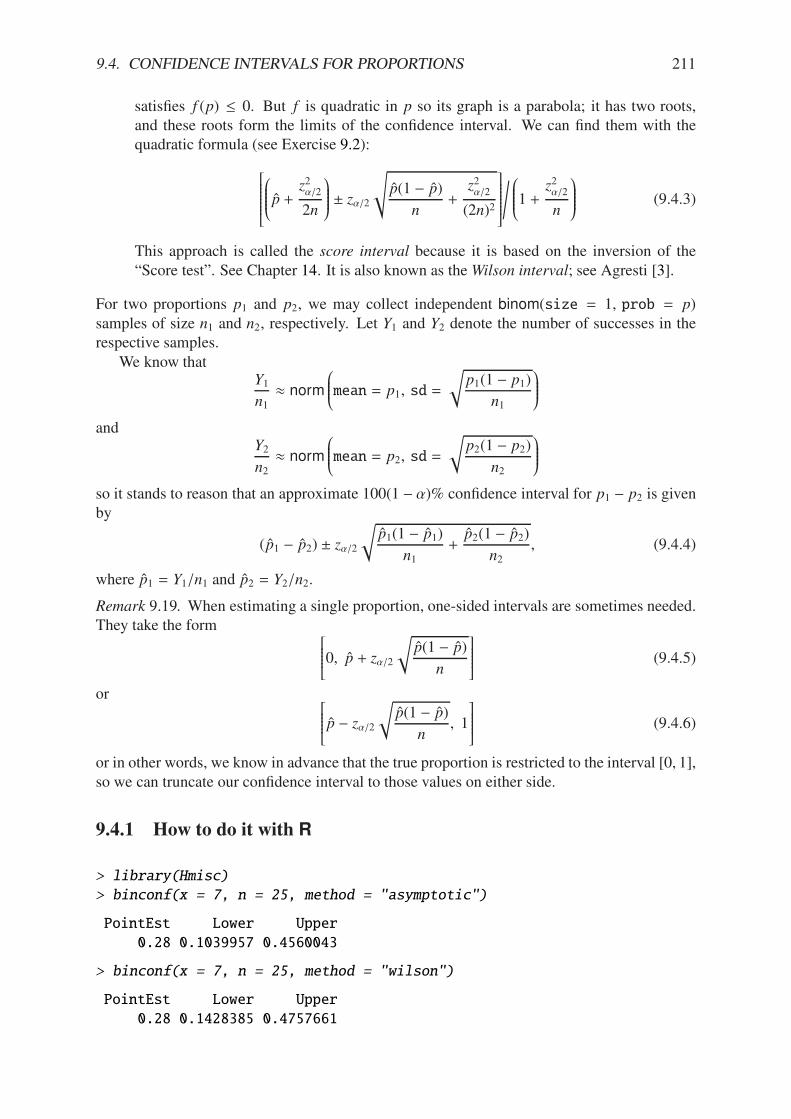
9.4. CONFIDENCE INTERVALS FOR PROPORTIONS 211
satisfies f (p) " 0. But f is quadratic in p so its graph is a parabola; it has two roots,and these roots form the limits of the confidence interval. We can find them with thequadratic formula (see Exercise 9.2):
EFFFFFFFFG
$%%%%%&p +
z2(/2
2n
()))))* ± z(/2
Xp(1 # p)
n+
z2(/2
(2n)2
HIIIIIIIIJ
Y $%%%%%&1 +
z2(/2
n
()))))* (9.4.3)
This approach is called the score interval because it is based on the inversion of the“Score test”. See Chapter 14. It is also known as theWilson interval; see Agresti [3].
For two proportions p1 and p2, we may collect independent binom(size = 1, prob = p)samples of size n1 and n2, respectively. Let Y1 and Y2 denote the number of successes in therespective samples.
We know thatY1
n1' norm
$%%%%&mean = p1, sd =
Up1(1 # p1)
n1
())))*
andY2
n2' norm
$%%%%&mean = p2, sd =
Up2(1 # p2)
n2
())))*
so it stands to reason that an approximate 100(1 # ()% confidence interval for p1 # p2 is givenby
(p1 # p2) ± z(/2
Up1(1 # p1)
n1+
p2(1 # p2)
n2, (9.4.4)
where p1 = Y1/n1 and p2 = Y2/n2.
Remark 9.19. When estimating a single proportion, one-sided intervals are sometimes needed.They take the form E
FFFFFG0, p + z(/2
Up(1 # p)
n
HIIIIIJ (9.4.5)
or EFFFFFGp # z(/2
Up(1 # p)
n, 1
HIIIIIJ (9.4.6)
or in other words, we know in advance that the true proportion is restricted to the interval [0, 1],so we can truncate our confidence interval to those values on either side.
9.4.1 How to do it with R
> library(Hmisc)
> binconf(x = 7, n = 25, method = "asymptotic")
PointEst Lower Upper
0.28 0.1039957 0.4560043
> binconf(x = 7, n = 25, method = "wilson")
PointEst Lower Upper
0.28 0.1428385 0.4757661

212 CHAPTER 9. ESTIMATION
The default value of the method argument is wilson.An alternate way is
> tab <- xtabs(~gender, data = RcmdrTestDrive)
> prop.test(rbind(tab), conf.level = 0.95, correct = FALSE)
1-sample proportions test without continuity correction
data: rbind(tab), null probability 0.5
X-squared = 2.881, df = 1, p-value = 0.08963
alternative hypothesis: true p is not equal to 0.5
95 percent confidence interval:
0.4898844 0.6381406
sample estimates:
p
0.5654762
> A <- as.data.frame(Titanic)
> library(reshape)
> B <- with(A, untable(A, Freq))
9.5 Confidence Intervals for Variances
I am thinking one and two sample problems here.
9.5.1 How to do it with R
I am thinking about sigma.test in the TeachingDemos package and var.test in base R here.
9.6 Fitting Distributions
9.6.1 How to do it with R
I am thinking about fitdistr from the MASS package [84].
9.7 Sample Size and Margin of Error
Sections 9.2 through 9.5 all began the same way: we were given the sample size n and theconfidence coe"cient 1 # (, and our task was to find a margin of error E so that
, ± E is a 100(1 # ()% confidence interval for ,.
Some examples we saw were:
• E = z(/2"/$n, in the one-sample z-interval,
• E = t(/2(df = n + m # 2)S p
$n#1 + m#1, in the two-sample pooled t-interval.
9.7. SAMPLE SIZE AND MARGIN OF ERROR 213
We already know (we can see in the formulas above) that E decreases as n increases. Now wewould like to use this information to our advantage: suppose that we have a fixed margin oferror E, say E = 3, and we want a 100(1#()% confidence interval for µ. The question is: howbig does n have to be?
For the case of a population mean the answer is easy: we set up an equation and solve forn.
Example 9.20. Given a situation, given ", given E, we would like to know how big n has to beto ensure that X ± 5 is a 95% confidence interval for µ.
Remark 9.21.
1. Always round up any decimal values of n, no matter how small the decimal is.
2. Another name for E is the “maximum error of the estimate”.
For proportions, recall that the asymptotic formula to estimate p was
p ± z(/2
Up(1 # p)
n.
Reasoning as above we would want
E = z(/2
Up(1 # p)
n, or (9.7.1)
n = z2(/2p(1 # p)
E2. (9.7.2)
OOPS! Recall that p = Y/n, which would put the variable n on both sides of Equation 9.7.2.Again, there are two solutions to the problem.
1. If we have a good idea of what p is, say p6 then we can plug it in to get
n = z2(/2p6(1 # p6)
E2. (9.7.3)
2. Even if we have no idea what p is, we do know from calculus that p(1 # p) " 1/4because the function f (x) = x(1 # x) is quadratic (so its graph is a parabola which opensdownward) with maximum value attained at x = 1/2. Therefore, regardless of our choicefor p6 the sample size must satisfy
n = z2(/2p6(1 # p6)
E2"
z2(/2
4E2. (9.7.4)
The quantity z2(/2/4E2 is large enough to guarantee 100(1 # ()% confidence.
Example 9.22. Proportion example
Remark 9.23. For very small populations sometimes the value of n obtained from the formulais too big. In this case we should use the hypergeometric distribution for a sampling modelrather than the binomial model. With this modification the formulas change to the following:if N denotes the population size then let
m = z2(/2p6(1 # p6)
E2(9.7.5)
and the sample size needed to ensure 100(1 # ()% confidence is achieved is
n =m
1 + m#1N
. (9.7.6)
If we do not have a good value for the estimate p6 then we may use p6 = 1/2.

214 CHAPTER 9. ESTIMATION
9.7.1 How to do it with R
I am thinking about power.t.test, power.prop.test, power.anova.test, and I am also thinking aboutreplicate.
9.8 Other Topics
Mention mle from the stats4 package.

9.8. OTHER TOPICS 215
Chapter Exercises
Exercise 9.1. Let X1, X2, . . . , Xn be an SRS (n) from a norm(mean = µ, sd = ") distribution.Find a two-dimensional MLE for , = (µ,").
Exercise 9.2. Find the upper and lower limits for the confidence interval procedure by findingthe roots of f defined by
f (p) = (Y/n # p)2 # z2(/2p(1 # p)
n.
You are going to need the quadratic formula.

216 CHAPTER 9. ESTIMATION
Chapter 10
Hypothesis Testing
What do I want them to know?
• basic terminology and philosophy of the Neyman-Pearson paradigm
• classical hypothesis tests for the standard one and two sample problems with means,variances, and proportions
• the notion of between versus within group variation and how it plays out with one-wayANOVA
• the concept of statistical power and its relation to sample size
10.1 Introduction
I spent a week during the summer of 2005 at the University of Nebraska at Lincoln grading Ad-vanced Placement Statistics exams, and while I was there I attended a presentation by Dr. RoxyPeck. At the end of her talk she described an activity she had used with students to introducethe basic concepts of hypothesis testing. I was impressed by the activity and have used it in myown classes several times since.
The instructor (with a box of cookies in hand) enters a class of fifteen or more students andproduces a brand-new, sealed deck of ordinary playing cards. The instructor asks for a studentvolunteer to break the seal, and then the instructor prominently shu#es the deck1 several timesin front of the class, after which time the students are asked to line up in a row. They are goingto play a game. Each student will draw a card from the top of the deck, in turn. If the card isblack, then the lucky student will get a cookie. If the card is red, then the unlucky student willsit down empty-handed. Let the game begin.
The first student draws a card: red. There are jeers and outbursts, and the student slinks o!to his/her chair. (S)he is disappointed, of course, but not really. After all, (s)he had a 50-50chance of getting black, and it did not happen. Oh well.
The second student draws a card: red, again. There are more jeers, and the second studentslips away. This student is also disappointed, but again, not so much, because it is probablyhis/her unlucky day. On to the next student.
The student draws: red again! There are a few wiseguys who yell (happy to make noise,more than anything else), but there are a few other students who are not yelling any more –they are thinking. This is the third red in a row, which is possible, of course, but what is going
1The jokers are removed before shu#ing.
217

218 CHAPTER 10. HYPOTHESIS TESTING
on, here? They are not quite sure. They are now concentrating on the next card. . . it is boundto be black, right?
The fourth student draws: red. Hmmm. . . now there are groans instead of outbursts. A fewof the students at the end of the line shrug their shoulders and start to make their way back totheir desk, complaining that the teacher does not want to give away any cookies. There are stillsome students in line though, salivating, waiting for the inevitable black to appear.
The fifth student draws red. Now it isn’t funny any more. As the remaining students maketheir way back to their seats an uproar ensues, from an entire classroom demanding cookies.
Keep the preceding experiment in the back of your mind as you read the following sections.When you have finished the entire chapter, come back and read this introduction again. All ofthe mathematical jargon that follows is connected to the above paragraphs. In the meantime, Iwill get you started:
Null hypothesis: it is an ordinary deck of playing cards, shu#ed thoroughly.
Alternative hypothesis: either it is a trick deck of cards, or the instructor did some fancyshu#ework.
Observed data: a sequence of draws from the deck, five reds in a row.
If it were truly an ordinary, well-shu#ed deck of cards, the probability of observing zero blacksout of a sample of size five (without replacement) from a deck with 26 black cards and 26 redcards would be
> dhyper(0, m = 26, n = 26, k = 5)
[1] 0.02531012
There are two very important final thoughts. First, everybody gets a cookie in the end.Second, the students invariably (and aggressively) attempt to get me to open up the deck andreveal the true nature of the cards. I never do.
10.2 Tests for Proportions
Example 10.1. We have a machine that makes widgets.
• Under normal operation, about 0.10 of the widgets produced are defective.
• Go out and purchase a torque converter.
• Install the torque converter, and observe n = 100 widgets from the machine.
• Let Y = number of defective widgets observed.
If
• Y = 0, then the torque converter is great!
• Y = 4, then the torque converter seems to be helping.
• Y = 9, then there is not much evidence that the torque converter helps.
10.2. TESTS FOR PROPORTIONS 219
• Y = 17, then throw away the torque converter.
Let p denote the proportion of defectives produced by the machine. Before the installation ofthe torque converter p was 0.10. Then we installed the torque converter. Did p change? Did itgo up or down? We use statistics to decide. Our method is to observe data and construct a 95%confidence interval for p,
p ± z(/2
Up(1 # p)
n. (10.2.1)
If the confidence interval is
• [0.01, 0.05], then we are 95% confident that 0.01 " p " 0.05, so there is evidence thatthe torque converter is helping.
• [0.15, 0.19], then we are 95% confident that 0.15 " p " 0.19, so there is evidence thatthe torque converter is hurting.
• [0.07, 0.11], then there is not enough evidence to conclude that the torque converter isdoing anything at all, positive or negative.
10.2.1 Terminology
The null hypothesis H0 is a “nothing” hypothesis, whose interpretation could be that nothinghas changed, there is no di!erence, there is nothing special taking place, etc.. In Example 10.1the null hypothesis would be H0 : p = 0.10. The alternative hypothesis H1 is the hypothesisthat something has changed, in this case, H1 : p ! 0.10. Our goal is to statistically test thehypothesis H0 : p = 0.10 versus the alternative H1 : p ! 0.10. Our procedure will be:
1. Go out and collect some data, in particular, a simple random sample of observations fromthe machine.
2. Suppose that H0 is true and construct a 100(1 # ()% confidence interval for p.
3. If the confidence interval does not cover p = 0.10, then we rejectH0. Otherwise, we failto rejectH0.
Remark 10.2. Every time we make a decision it is possible to be wrong, and there are twopossible mistakes that we could make. We have committed a
Type I Error if we reject H0 when in fact H0 is true. This would be akin to convicting aninnocent person for a crime (s)he did not commit.
Type II Error if we fail to reject H0 when in fact H1 is true. This is analogous to a guiltyperson escaping conviction.
Type I Errors are usually considered worse2, and we design our statistical procedures to controlthe probability of making such a mistake. We define the
significance level of the test = IP(Type I Error) = (. (10.2.2)
We want ( to be small which conventionally means, say, ( = 0.05, ( = 0.01, or ( = 0.005 (butcould mean anything, in principle).
2There is no mathematical di!erence between the errors, however. The bottom line is that we choose one typeof error to control with an iron fist, and we try to minimize the probability of making the other type. That beingsaid, null hypotheses are often by design to correspond to the “simpler” model, so it is often easier to analyze (andthereby control) the probabilities associated with Type I Errors.

220 CHAPTER 10. HYPOTHESIS TESTING
• The rejection region (also known as the critical region) for the test is the set of samplevalues which would result in the rejection of H0. For Example 10.1, the rejection regionwould be all possible samples that result in a 95% confidence interval that does not coverp = 0.10.
• The above example with H1 : p ! 0.10 is called a two-sided test. Many times we areinterested in a one-sided test, which would look like H1 : p < 0.10 or H1 : p > 0.10.
We are ready for tests of hypotheses for one proportion.Table here.Don’t forget the assumptions.
Example 10.3. Find
1. The null and alternative hypotheses
2. Check your assumptions.
3. Define a critical region with an ( = 0.05 significance level.
4. Calculate the value of the test statistic and state your conclusion.
Example 10.4. Suppose p = the proportion of students who are admitted to the graduateschool of the University of California at Berkeley, and suppose that a public relations o"cerboasts that UCB has historically had a 40% acceptance rate for its graduate school. Considerthe data stored in the table UCBAdmissions from 1973. Assuming these observations consti-tuted a simple random sample, are they consistent with the o"cer’s claim, or do they provideevidence that the acceptance rate was significantly less than 40%? Use an ( = 0.01 significancelevel.
Our null hypothesis in this problem is H0 : p = 0.4 and the alternative hypothesis isH1 : p < 0.4. We reject the null hypothesis if p is too small, that is, if
p # 0.4$0.4(1 # 0.4)/n
< #z(, (10.2.3)
where ( = 0.01 and #z0.01 is
> -qnorm(0.99)
[1] -2.326348
Our only remaining task is to find the value of the test statistic and see where it falls relativeto the critical value. We can find the number of people admitted and not admitted to the UCBgraduate school with the following.
> A <- as.data.frame(UCBAdmissions)
> head(A)
Admit Gender Dept Freq
1 Admitted Male A 512
2 Rejected Male A 313
3 Admitted Female A 89
4 Rejected Female A 19
5 Admitted Male B 353
6 Rejected Male B 207
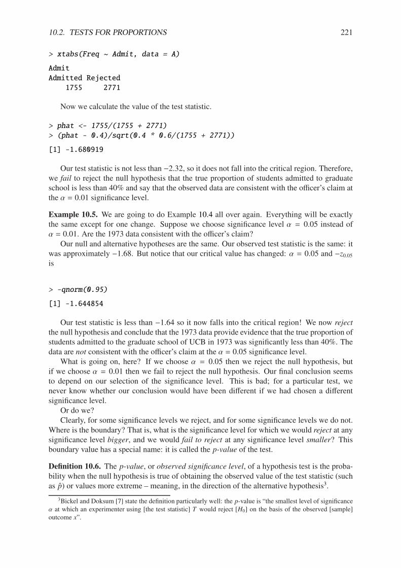
10.2. TESTS FOR PROPORTIONS 221
> xtabs(Freq ~ Admit, data = A)
Admit
Admitted Rejected
1755 2771
Now we calculate the value of the test statistic.
> phat <- 1755/(1755 + 2771)
> (phat - 0.4)/sqrt(0.4 * 0.6/(1755 + 2771))
[1] -1.680919
Our test statistic is not less than #2.32, so it does not fall into the critical region. Therefore,we fail to reject the null hypothesis that the true proportion of students admitted to graduateschool is less than 40% and say that the observed data are consistent with the o"cer’s claim atthe ( = 0.01 significance level.
Example 10.5. We are going to do Example 10.4 all over again. Everything will be exactlythe same except for one change. Suppose we choose significance level ( = 0.05 instead of( = 0.01. Are the 1973 data consistent with the o"cer’s claim?
Our null and alternative hypotheses are the same. Our observed test statistic is the same: itwas approximately #1.68. But notice that our critical value has changed: ( = 0.05 and #z0.05is
> -qnorm(0.95)
[1] -1.644854
Our test statistic is less than #1.64 so it now falls into the critical region! We now reject
the null hypothesis and conclude that the 1973 data provide evidence that the true proportion ofstudents admitted to the graduate school of UCB in 1973 was significantly less than 40%. Thedata are not consistent with the o"cer’s claim at the ( = 0.05 significance level.
What is going on, here? If we choose ( = 0.05 then we reject the null hypothesis, butif we choose ( = 0.01 then we fail to reject the null hypothesis. Our final conclusion seemsto depend on our selection of the significance level. This is bad; for a particular test, wenever know whether our conclusion would have been di!erent if we had chosen a di!erentsignificance level.
Or do we?Clearly, for some significance levels we reject, and for some significance levels we do not.
Where is the boundary? That is, what is the significance level for which we would reject at anysignificance level bigger, and we would fail to reject at any significance level smaller? Thisboundary value has a special name: it is called the p-value of the test.
Definition 10.6. The p-value, or observed significance level, of a hypothesis test is the proba-bility when the null hypothesis is true of obtaining the observed value of the test statistic (suchas p) or values more extreme – meaning, in the direction of the alternative hypothesis3.
3Bickel and Doksum [7] state the definition particularly well: the p-value is “the smallest level of significance( at which an experimenter using [the test statistic] T would reject [H0] on the basis of the observed [sample]outcome x”.
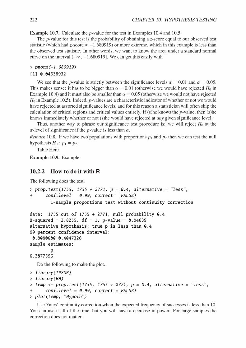
222 CHAPTER 10. HYPOTHESIS TESTING
Example 10.7. Calculate the p-value for the test in Examples 10.4 and 10.5.The p-value for this test is the probability of obtaining a z-score equal to our observed test
statistic (which had z-score ' #1.680919) or more extreme, which in this example is less thanthe observed test statistic. In other words, we want to know the area under a standard normalcurve on the interval (#&, #1.680919]. We can get this easily with
> pnorm(-1.680919)
[1] 0.04638932
We see that the p-value is strictly between the significance levels ( = 0.01 and ( = 0.05.This makes sense: it has to be bigger than ( = 0.01 (otherwise we would have rejected H0 inExample 10.4) and it must also be smaller than ( = 0.05 (otherwise we would not have rejectedH0 in Example 10.5). Indeed, p-values are a characteristic indicator of whether or not we wouldhave rejected at assorted significance levels, and for this reason a statistician will often skip thecalculation of critical regions and critical values entirely. If (s)he knows the p-value, then (s)heknows immediately whether or not (s)he would have rejected at any given significance level.
Thus, another way to phrase our significance test procedure is: we will reject H0 at the(-level of significance if the p-value is less than (.
Remark 10.8. If we have two populations with proportions p1 and p2 then we can test the nullhypothesis H0 : p1 = p2.
Table Here.
Example 10.9. Example.
10.2.2 How to do it with R
The following does the test.
> prop.test(1755, 1755 + 2771, p = 0.4, alternative = "less",
+ conf.level = 0.99, correct = FALSE)
1-sample proportions test without continuity correction
data: 1755 out of 1755 + 2771, null probability 0.4
X-squared = 2.8255, df = 1, p-value = 0.04639
alternative hypothesis: true p is less than 0.4
99 percent confidence interval:
0.0000000 0.4047326
sample estimates:
p
0.3877596
Do the following to make the plot.
> library(IPSUR)
> library(HH)
> temp <- prop.test(1755, 1755 + 2771, p = 0.4, alternative = "less",
+ conf.level = 0.99, correct = FALSE)
> plot(temp, "Hypoth")
Use Yates’ continuity correction when the expected frequency of successes is less than 10.You can use it all of the time, but you will have a decrease in power. For large samples thecorrection does not matter.
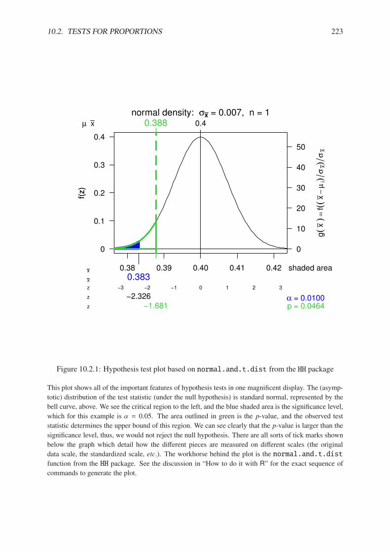
10.2. TESTS FOR PROPORTIONS 223
0.38 0.39 0.40 0.41 0.42
normal density: "x = 0.007, n = 1
f(z)
0
10
20
30
40
50
!3 !2 !1 0 1 2 3
0
0.1
0.2
0.3
0.4
g(
x )
=f(
( x#
µ i)
" x)"
x
f(z)
!2.326z
z
shaded area
$ = 0.0100
0.383x
x
µ x 0.40.388
!1.681z p = 0.0464
Figure 10.2.1: Hypothesis test plot based on normal.and.t.dist from the HH package
This plot shows all of the important features of hypothesis tests in one magnificent display. The (asymp-
totic) distribution of the test statistic (under the null hypothesis) is standard normal, represented by the
bell curve, above. We see the critical region to the left, and the blue shaded area is the significance level,
which for this example is ( = 0.05. The area outlined in green is the p-value, and the observed test
statistic determines the upper bound of this region. We can see clearly that the p-value is larger than the
significance level, thus, we would not reject the null hypothesis. There are all sorts of tick marks shown
below the graph which detail how the di!erent pieces are measured on di!erent scales (the original
data scale, the standardized scale, etc.). The workhorse behind the plot is the normal.and.t.dist
function from the HH package. See the discussion in “How to do it with R” for the exact sequence of
commands to generate the plot.
224 CHAPTER 10. HYPOTHESIS TESTING
With the R Commander If you already know the number of successes and failures, then youcan use the menu Statistics ! Proportions ! IPSUR Enter table for single sample. . .
Otherwise, your data – the raw successes and failures – should be in a column of the ActiveData Set. Furthermore, the data must be stored as a “factor” internally. If the data are not afactor but are numeric then you can use the menu Data ! Manage variables in active dataset ! Convert numeric variables to factors. . . to convert the variable to a factor. Or, you canalways use the factor function.
Once your unsummarized data is a column, then you can use the menu Statistics ! Propor-tions ! Single-sample proportion test. . .
10.3 One Sample Tests for Means and Variances
10.3.1 For Means
Here, X1, X2, . . . , Xn are a SRS (n) from a norm(mean = µ, sd = ") distribution. We wouldlike to test H0 : µ = µ0.
Case A: Suppose " is known. Then under H0,
Z =X # µ0"/
$n4 norm(mean = 0, sd = 1).
Table here.
Case B: When " is unknown, under H0
T =X # µ0S/
$n
4 t(df = n # 1).
Table here.
Remark 10.10. If " is unknown but n is large then we can use the z-test.
Example 10.11. In this example we
1. Find the null and alternative hypotheses.
2. Choose a test and find the critical region.
3. Calculate the value of the test statistic and state the conclusion.
4. Find the p-value.
Remark 10.12. Remarks
• p-values are also known as tail end probabilities. We reject H0 when the p-value is small.
• "/$n when " is known, is called the standard error of the sample mean. In general,
if we have an estimator , then ", is called the standard error of ,. We usually need toestimate ", with ",.
10.3. ONE SAMPLE TESTS FOR MEANS AND VARIANCES 225
10.3.2 How to do it with R
I am thinking z.test in TeachingDemos, t.test in base R.
> x <- rnorm(37, mean = 2, sd = 3)
> library(TeachingDemos)
> z.test(x, mu = 1, sd = 3, conf.level = 0.9)
One Sample z-test
data: x
z = 2.8126, n = 37.000, Std. Dev. = 3.000, Std. Dev. of the sample
mean = 0.493, p-value = 0.004914
alternative hypothesis: true mean is not equal to 1
90 percent confidence interval:
1.575948 3.198422
sample estimates:
mean of x
2.387185
The RcmdrPlugin.IPSUR package does not have a menu for z.test yet.
> x <- rnorm(13, mean = 2, sd = 3)
> t.test(x, mu = 0, conf.level = 0.9, alternative = "greater")
One Sample t-test
data: x
t = 1.2949, df = 12, p-value = 0.1099
alternative hypothesis: true mean is greater than 0
90 percent confidence interval:
-0.05064006 Inf
sample estimates:
mean of x
1.068850
With the R Commander Your data should be in a single numeric column (a variable) of theActive Data Set. Use the menu Statistics ! Means ! Single-sample t-test. . .
10.3.3 Tests for a Variance
Here, X1, X2, . . . , Xn are a SRS (n) from a norm(mean = µ, sd = ") distribution. We wouldlike to test H0 : "
2 = "0. We know that under H0,
X2 =(n # 1)S 2
"24 chisq(df = n # 1).
Table here.
Example 10.13. Give some data and a hypothesis.
1. Give an (-level and test the critical region way.
2. Find the p-value for the test.
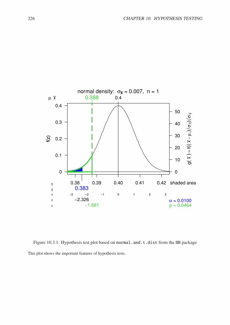
226 CHAPTER 10. HYPOTHESIS TESTING
0.38 0.39 0.40 0.41 0.42
normal density: "x = 0.007, n = 1
f(z)
0
10
20
30
40
50
!3 !2 !1 0 1 2 3
0
0.1
0.2
0.3
0.4
g(
x )
=f(
( x#
µ i)
" x)"
x
f(z)
!2.326z
z
shaded area
$ = 0.0100
0.383x
x
µ x 0.40.388
!1.681z p = 0.0464
Figure 10.3.1: Hypothesis test plot based on normal.and.t.dist from the HH package
This plot shows the important features of hypothesis tests.
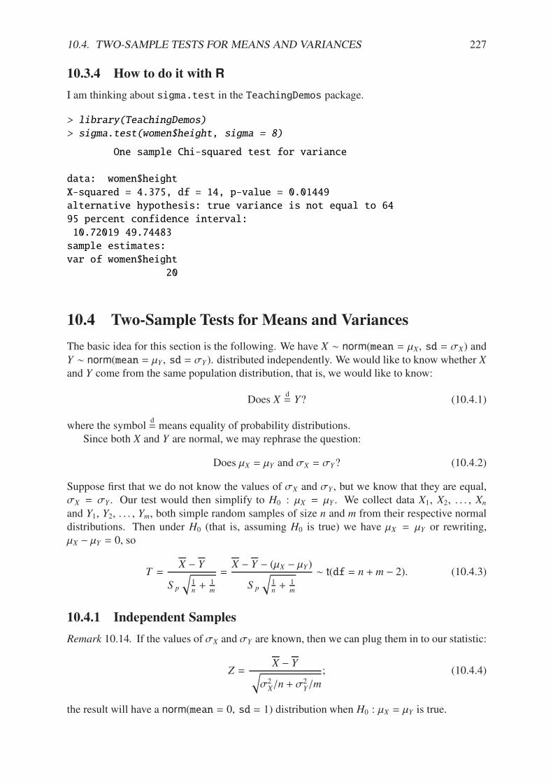
10.4. TWO-SAMPLE TESTS FOR MEANS AND VARIANCES 227
10.3.4 How to do it with R
I am thinking about sigma.test in the TeachingDemos package.
> library(TeachingDemos)
> sigma.test(women$height, sigma = 8)
One sample Chi-squared test for variance
data: women$height
X-squared = 4.375, df = 14, p-value = 0.01449
alternative hypothesis: true variance is not equal to 64
95 percent confidence interval:
10.72019 49.74483
sample estimates:
var of women$height
20
10.4 Two-Sample Tests for Means and Variances
The basic idea for this section is the following. We have X 4 norm(mean = µX, sd = "X) andY 4 norm(mean = µY , sd = "Y). distributed independently. We would like to know whether Xand Y come from the same population distribution, that is, we would like to know:
Does Xd= Y? (10.4.1)
where the symbold= means equality of probability distributions.
Since both X and Y are normal, we may rephrase the question:
Does µX = µY and "X = "Y? (10.4.2)
Suppose first that we do not know the values of "X and "Y , but we know that they are equal,"X = "Y . Our test would then simplify to H0 : µX = µY . We collect data X1, X2, . . . , Xn
and Y1, Y2, . . . , Ym, both simple random samples of size n and m from their respective normaldistributions. Then under H0 (that is, assuming H0 is true) we have µX = µY or rewriting,µX # µY = 0, so
T =X # Y
S p
M1n+ 1
m
=X # Y # (µX # µY )
S p
M1n+ 1
m
4 t(df = n + m # 2). (10.4.3)
10.4.1 Independent Samples
Remark 10.14. If the values of "X and "Y are known, then we can plug them in to our statistic:
Z =X # Y
M"2
X/n + "2Y/m
; (10.4.4)
the result will have a norm(mean = 0, sd = 1) distribution when H0 : µX = µY is true.
228 CHAPTER 10. HYPOTHESIS TESTING
Remark 10.15. Even if the values of "X and "Y are not known, if both n and m are large thenwe can plug in the sample estimates and the result will have approximately a norm(mean =0, sd = 1) distribution when H0 : µX = µY is true.
Z =X # Y
MS 2
X/n + S2Y/m
. (10.4.5)
Remark 10.16. It is usually important to construct side-by-side boxplots and other visual dis-plays in concert with the hypothesis test. This gives a visual comparison of the samples andhelps to identify departures from the test’s assumptions – such as outliers.
Remark 10.17. WATCH YOUR ASSUMPTIONS.
• The normality assumption can be relaxed as long as the population distributions are nothighly skewed.
• The equal variance assumption can be relaxed as long as both sample sizes n and m arelarge. However, if one (or both) samples is small, then the test does not perform well; weshould instead use the methods of Chapter 13.
For a nonparametric alternative to the two-sample F test see Chapter 15.
10.4.2 Paired Samples
10.4.3 How to do it with R
> t.test(extra ~ group, data = sleep, paired = TRUE)
Paired t-test
data: extra by group
t = -4.0621, df = 9, p-value = 0.002833
alternative hypothesis: true difference in means is not equal to 0
95 percent confidence interval:
-2.4598858 -0.7001142
sample estimates:
mean of the differences
-1.58
10.5 Other Hypothesis Tests
10.5.1 Kolmogorov-Smirnov Goodness-of-Fit Test
10.5.2 How to do it with R
> ks.test(randu$x, "punif")
One-sample Kolmogorov-Smirnov test
data: randu$x
D = 0.0555, p-value = 0.1697
alternative hypothesis: two-sided
10.6. ANALYSIS OF VARIANCE 229
10.5.3 Shapiro-Wilk Normality Test
10.5.4 How to do it with R
> shapiro.test(women$height)
Shapiro-Wilk normality test
data: women$height
W = 0.9636, p-value = 0.7545
10.6 Analysis of Variance
10.6.1 How to do it with R
I am thinking
> with(chickwts, by(weight, feed, shapiro.test))
feed: casein
Shapiro-Wilk normality test
data: dd[x, ]
W = 0.9166, p-value = 0.2592
--------------------------------------------------------
feed: horsebean
Shapiro-Wilk normality test
data: dd[x, ]
W = 0.9376, p-value = 0.5265
--------------------------------------------------------
feed: linseed
Shapiro-Wilk normality test
data: dd[x, ]
W = 0.9693, p-value = 0.9035
--------------------------------------------------------
feed: meatmeal
Shapiro-Wilk normality test
data: dd[x, ]
230 CHAPTER 10. HYPOTHESIS TESTING
W = 0.9791, p-value = 0.9612
--------------------------------------------------------
feed: soybean
Shapiro-Wilk normality test
data: dd[x, ]
W = 0.9464, p-value = 0.5064
--------------------------------------------------------
feed: sunflower
Shapiro-Wilk normality test
data: dd[x, ]
W = 0.9281, p-value = 0.3603
and
> temp <- lm(weight ~ feed, data = chickwts)
and
> anova(temp)
Analysis of Variance Table
Response: weight
Df Sum Sq Mean Sq F value Pr(>F)
feed 5 231129 46226 15.365 5.936e-10 ***
Residuals 65 195556 3009
---
Signif. codes: 0 '***' 0.001 '**' 0.01 '*' 0.05 '.' 0.1 ' ' 1
Plot for the intuition of between versus within group variation.Plots for the hypothesis tests:
10.7 Sample Size and Power
The power function of a test for a parameter , is
*(,) = IP,(Reject H0), #& < , < &.
Here are some properties of power functions:
1. *(,) " ( for any , 3 '0, and *(,0) = (. We interpret this by saying that no matter whatvalue , takes inside the null parameter space, there is never more than a chance of ( ofrejecting the null hypothesis. We have controlled the Type I error rate to be no greaterthan (.
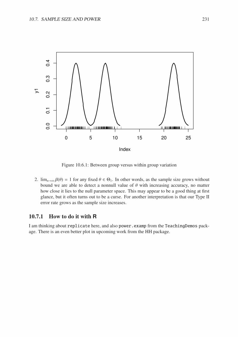
10.7. SAMPLE SIZE AND POWER 231
0 5 10 15 20 25
0.0
0.1
0.2
0.3
0.4
Index
y1
Figure 10.6.1: Between group versus within group variation
2. limn.& *(,) = 1 for any fixed , 3 '1. In other words, as the sample size grows withoutbound we are able to detect a nonnull value of , with increasing accuracy, no matterhow close it lies to the null parameter space. This may appear to be a good thing at firstglance, but it often turns out to be a curse. For another interpretation is that our Type IIerror rate grows as the sample size increases.
10.7.1 How to do it with R
I am thinking about replicate here, and also power.examp from the TeachingDemos pack-age. There is an even better plot in upcoming work from the HH package.
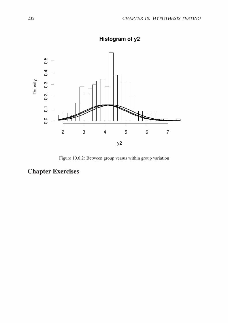
232 CHAPTER 10. HYPOTHESIS TESTING
Histogram of y2
y2
Densi
ty
2 3 4 5 6 7
0.0
0.1
0.2
0.3
0.4
0.5
Figure 10.6.2: Between group versus within group variation
Chapter Exercises
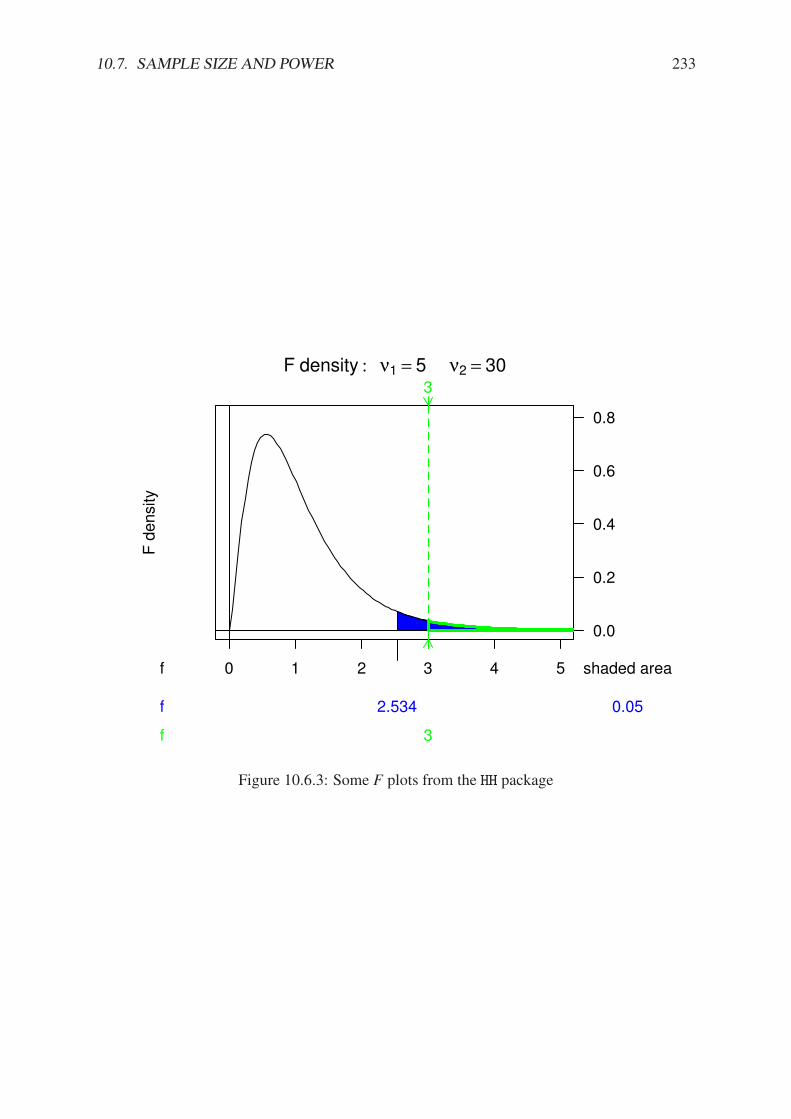
10.7. SAMPLE SIZE AND POWER 233
0 1 2 3 4 5
F density : %1 = 5 %2 = 30
F d
ensi
ty
0.0
0.2
0.4
0.6
0.8
f
2.534f
shaded area
0.05
3
3f
Figure 10.6.3: Some F plots from the HH package
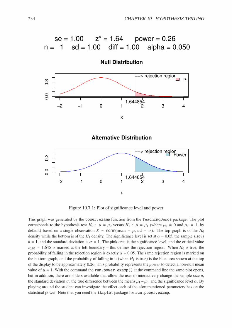
234 CHAPTER 10. HYPOTHESIS TESTING
!2 !1 0 1 2 3 4
0.0
0.3
Null Distribution
x
!!> rejection region
1.644854
$
!2 !1 0 1 2 3 4
0.0
0.3
Alternative Distribution
x
!!> rejection region
1.644854
Power
se = 1.00 z* = 1.64 power = 0.26 n = 1 sd = 1.00 diff = 1.00 alpha = 0.050
Figure 10.7.1: Plot of significance level and power
This graph was generated by the power.examp function from the TeachingDemos package. The plot
corresponds to the hypothesis test H0 : µ = µ0 versus H1 : µ = µ1 (where µ0 = 0 and µ1 = 1, by
default) based on a single observation X 4 norm(mean = µ, sd = "). The top graph is of the H0
density while the bottom is of the H1 density. The significance level is set at ( = 0.05, the sample size is
n = 1, and the standard deviation is " = 1. The pink area is the significance level, and the critical value
z0.05 ' 1.645 is marked at the left boundary – this defines the rejection region. When H0 is true, the
probability of falling in the rejection region is exactly ( = 0.05. The same rejection region is marked on
the bottom graph, and the probability of falling in it (when H1 is true) is the blue area shown at the top
of the display to be approximately 0.26. This probability represents the power to detect a non-null mean
value of µ = 1. With the command the run.power.examp() at the command line the same plot opens,
but in addition, there are sliders available that allow the user to interactively change the sample size n,
the standard deviation ", the true di!erence between the means µ1 #µ0, and the significance level (. Byplaying around the student can investigate the e!ect each of the aforementioned parameters has on the
statistical power. Note that you need the tkrplot package for run.power.examp.
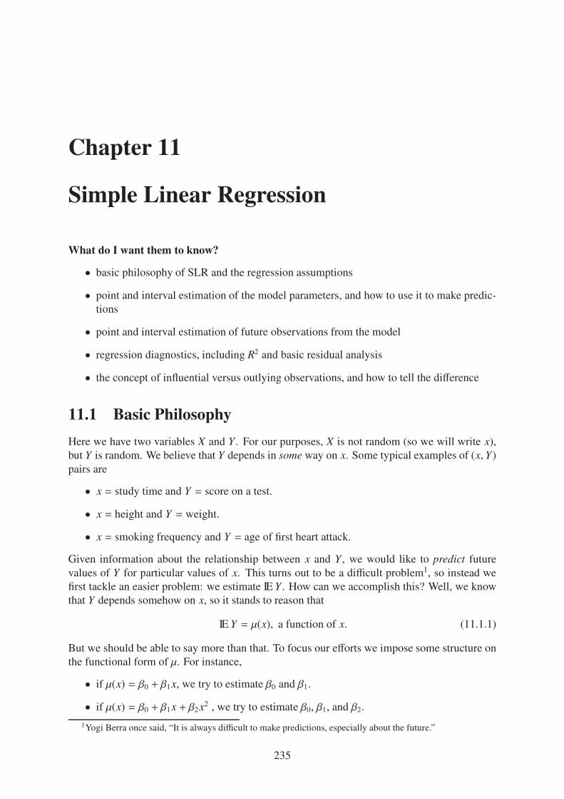
Chapter 11
Simple Linear Regression
What do I want them to know?
• basic philosophy of SLR and the regression assumptions
• point and interval estimation of the model parameters, and how to use it to make predic-tions
• point and interval estimation of future observations from the model
• regression diagnostics, including R2 and basic residual analysis
• the concept of influential versus outlying observations, and how to tell the di!erence
11.1 Basic Philosophy
Here we have two variables X and Y . For our purposes, X is not random (so we will write x),but Y is random. We believe that Y depends in some way on x. Some typical examples of (x, Y)pairs are
• x = study time and Y = score on a test.
• x = height and Y = weight.
• x = smoking frequency and Y = age of first heart attack.
Given information about the relationship between x and Y , we would like to predict futurevalues of Y for particular values of x. This turns out to be a di"cult problem1, so instead wefirst tackle an easier problem: we estimate IEY . How can we accomplish this? Well, we knowthat Y depends somehow on x, so it stands to reason that
IE Y = µ(x), a function of x. (11.1.1)
But we should be able to say more than that. To focus our e!orts we impose some structure onthe functional form of µ. For instance,
• if µ(x) = *0 + *1x, we try to estimate *0 and *1.
• if µ(x) = *0 + *1x + *2x2 , we try to estimate *0, *1, and *2.
1Yogi Berra once said, “It is always di"cult to make predictions, especially about the future.”
235
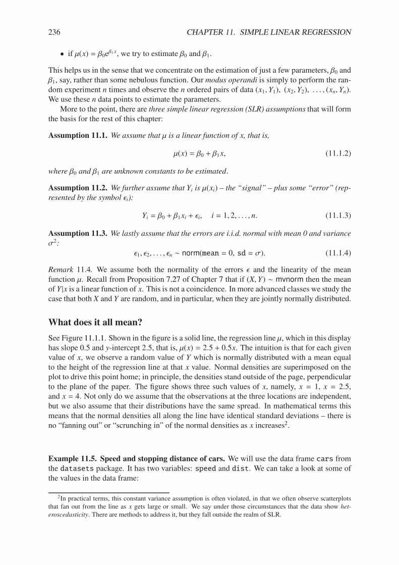
236 CHAPTER 11. SIMPLE LINEAR REGRESSION
• if µ(x) = *0e*1x, we try to estimate *0 and *1.
This helps us in the sense that we concentrate on the estimation of just a few parameters, *0 and*1, say, rather than some nebulous function. Our modus operandi is simply to perform the ran-dom experiment n times and observe the n ordered pairs of data (x1, Y1), (x2, Y2), . . . , (xn, Yn).We use these n data points to estimate the parameters.
More to the point, there are three simple linear regression (SLR) assumptions that will formthe basis for the rest of this chapter:
Assumption 11.1. We assume that µ is a linear function of x, that is,
µ(x) = *0 + *1x, (11.1.2)
where *0 and *1 are unknown constants to be estimated.
Assumption 11.2. We further assume that Yi is µ(xi) – the “signal” – plus some “error” (rep-
resented by the symbol $i):
Yi = *0 + *1xi + $i, i = 1, 2, . . . , n. (11.1.3)
Assumption 11.3. We lastly assume that the errors are i.i.d. normal with mean 0 and variance"2:
$1, $2, . . . , $n 4 norm(mean = 0, sd = "). (11.1.4)
Remark 11.4. We assume both the normality of the errors $ and the linearity of the meanfunction µ. Recall from Proposition 7.27 of Chapter 7 that if (X, Y) 4 mvnorm then the meanof Y |x is a linear function of x. This is not a coincidence. In more advanced classes we study thecase that both X and Y are random, and in particular, when they are jointly normally distributed.
What does it all mean?
See Figure 11.1.1. Shown in the figure is a solid line, the regression line µ, which in this displayhas slope 0.5 and y-intercept 2.5, that is, µ(x) = 2.5 + 0.5x. The intuition is that for each givenvalue of x, we observe a random value of Y which is normally distributed with a mean equalto the height of the regression line at that x value. Normal densities are superimposed on theplot to drive this point home; in principle, the densities stand outside of the page, perpendicularto the plane of the paper. The figure shows three such values of x, namely, x = 1, x = 2.5,and x = 4. Not only do we assume that the observations at the three locations are independent,but we also assume that their distributions have the same spread. In mathematical terms thismeans that the normal densities all along the line have identical standard deviations – there isno “fanning out” or “scrunching in” of the normal densities as x increases2.
Example 11.5. Speed and stopping distance of cars. We will use the data frame cars fromthe datasets package. It has two variables: speed and dist. We can take a look at some ofthe values in the data frame:
2In practical terms, this constant variance assumption is often violated, in that we often observe scatterplotsthat fan out from the line as x gets large or small. We say under those circumstances that the data show het-
eroscedasticity. There are methods to address it, but they fall outside the realm of SLR.
11.1. BASIC PHILOSOPHY 237
0 1 2 3 4 5
01
23
45
6
x
y
Figure 11.1.1: Philosophical foundations of SLR
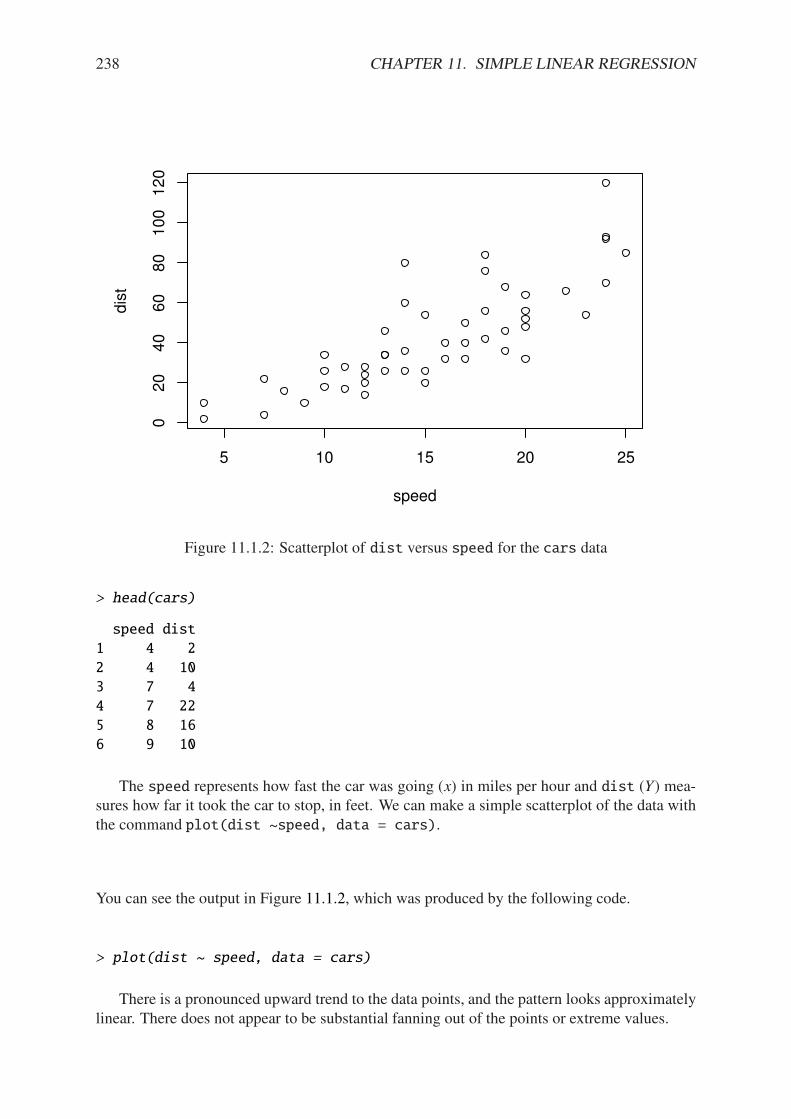
238 CHAPTER 11. SIMPLE LINEAR REGRESSION
5 10 15 20 25
020
40
60
80
100
120
speed
dis
t
Figure 11.1.2: Scatterplot of dist versus speed for the cars data
> head(cars)
speed dist
1 4 2
2 4 10
3 7 4
4 7 22
5 8 16
6 9 10
The speed represents how fast the car was going (x) in miles per hour and dist (Y) mea-sures how far it took the car to stop, in feet. We can make a simple scatterplot of the data withthe command plot(dist ~speed, data = cars).
You can see the output in Figure 11.1.2, which was produced by the following code.
> plot(dist ~ speed, data = cars)
There is a pronounced upward trend to the data points, and the pattern looks approximatelylinear. There does not appear to be substantial fanning out of the points or extreme values.

11.2. ESTIMATION 239
11.2 Estimation
11.2.1 Point Estimates of the Parameters
Where is µ(x)? In essence, we would like to “fit” a line to the points. But how do we determinea “good” line? Is there a best line? We will use maximum likelihood to find it. We know:
Yi = *0 + *1xi + $i, i = 1, . . . , n, (11.2.1)
where the $i’s are i.i.d. norm(mean = 0, sd = "). Thus Yi 4 norm(mean = *0 + *1xi, sd ="), i = 1, . . . , n. Furthermore, Y1, . . . , Yn are independent – but not identically distributed. Thelikelihood function is:
L(*0, *1,") =nW
i=1
fYi(yi), (11.2.2)
=
nW
i=1
(2&"2)#1/2 exp
.#(yi # *0 # *1xi)2
2"2
/, (11.2.3)
=(2&"2)#n/2 exp
.#
#ni=1(yi # *0 # *1xi)
2
2"2
/. (11.2.4)
We take the natural logarithm to get
ln L(*0, *1,") = #n
2ln(2&"2) #
#ni=1(yi # *0 # *1xi)2
2"2. (11.2.5)
We would like to maximize this function of *0 and *1. See Appendix E.6 which tells us thatwe should find critical points by means of the partial derivatives. Let us start by di!erentiatingwith respect to *0:
-
-*0ln L = 0 #
1
2"2
n!
i=1
2(yi # *0 # *1xi)(#1), (11.2.6)
and the partial derivative equals zero when#n
i=1(yi # *0 # *1xi) = 0, that is, when
n*0 + *1
n!
i=1
xi =
n!
i=1
yi. (11.2.7)
Moving on, we next take the partial derivative of ln L (Equation 11.2.5) with respect to *1 toget
-
-*1ln L = 0 #
1
2"2
n!
i=1
2(yi # *0 # *1xi)(#xi), (11.2.8)
=1
"2
n!
i=1
2xiyi # *0xi # *1x2i
3, (11.2.9)
and this equals zero when the last sum equals zero, that is, when
*0
n!
i=1
xi + *1
n!
i=1
x2i =
n!
i=1
xiyi. (11.2.10)
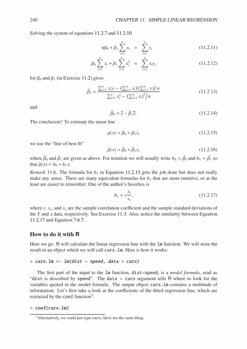
240 CHAPTER 11. SIMPLE LINEAR REGRESSION
Solving the system of equations 11.2.7 and 11.2.10
n*0 + *1
n!
i=1
xi =
n!
i=1
yi (11.2.11)
*0
n!
i=1
xi + *1
n!
i=1
x2i =
n!
i=1
xiyi (11.2.12)
for *0 and *1 (in Exercise 11.2) gives
*1 =
#ni=1 xiyi #
=#ni=1 xi
> =#ni=1 yi
>Zn
#ni=1 x
2i #
=#ni=1 xi
>2Tn
(11.2.13)
and*0 = y # *1x. (11.2.14)
The conclusion? To estimate the mean line
µ(x) = *0 + *1x, (11.2.15)
we use the “line of best fit”µ(x) = *0 + *1x, (11.2.16)
where *0 and *1 are given as above. For notation we will usually write b0 = *0 and b1 = *1 sothat µ(x) = b0 + b1x.
Remark 11.6. The formula for b1 in Equation 11.2.13 gets the job done but does not reallymake any sense. There are many equivalent formulas for b1 that are more intuitive, or at theleast are easier to remember. One of the author’s favorites is
b1 = rsy
sx, (11.2.17)
where r, sy, and sx are the sample correlation coe"cient and the sample standard deviations ofthe Y and x data, respectively. See Exercise 11.3. Also, notice the similarity between Equation11.2.17 and Equation 7.6.7.
How to do it with R
Here we go. R will calculate the linear regression line with the lm function. We will store theresult in an object which we will call cars.lm. Here is how it works:
> cars.lm <- lm(dist ~ speed, data = cars)
The first part of the input to the lm function, dist~speed, is a model formula, read as“dist is described by speed”. The data = cars argument tells R where to look for thevariables quoted in the model formula. The output object cars.lm contains a multitude ofinformation. Let’s first take a look at the coe"cients of the fitted regression line, which areextracted by the coef function3:
> coef(cars.lm)
3Alternatively, we could just type cars.lm to see the same thing.
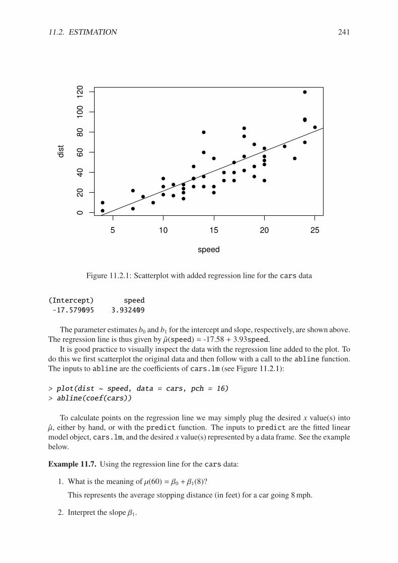
11.2. ESTIMATION 241
5 10 15 20 25
020
40
60
80
100
120
speed
dis
t
Figure 11.2.1: Scatterplot with added regression line for the cars data
(Intercept) speed
-17.579095 3.932409
The parameter estimates b0 and b1 for the intercept and slope, respectively, are shown above.The regression line is thus given by µ(speed) = -17.58 + 3.93speed.
It is good practice to visually inspect the data with the regression line added to the plot. Todo this we first scatterplot the original data and then follow with a call to the abline function.The inputs to abline are the coe"cients of cars.lm (see Figure 11.2.1):
> plot(dist ~ speed, data = cars, pch = 16)
> abline(coef(cars))
To calculate points on the regression line we may simply plug the desired x value(s) intoµ, either by hand, or with the predict function. The inputs to predict are the fitted linearmodel object, cars.lm, and the desired x value(s) represented by a data frame. See the examplebelow.
Example 11.7. Using the regression line for the cars data:
1. What is the meaning of µ(60) = *0 + *1(8)?
This represents the average stopping distance (in feet) for a car going 8mph.
2. Interpret the slope *1.
242 CHAPTER 11. SIMPLE LINEAR REGRESSION
The true slope *1 represents the increase in average stopping distance for each mile perhour faster that the car drives. In this case, we estimate the car to take approximately3.93 additional feet to stop for each additional mph increase in speed.
3. Interpret the intercept *0.
This would represent the mean stopping distance for a car traveling 0mph (which ourregression line estimates to be -17.58). Of course, this interpretation does not make anysense for this example, because a car travelling 0mph takes 0 ft to stop (it was not movingin the first place)! What went wrong? Looking at the data, we notice that the smallestspeed for which we have measured data is 4mph. Therefore, if we predict what wouldhappen for slower speeds then we would be extrapolating, a dangerous practice whichoften gives nonsensical results.
11.2.2 Point Estimates of the Regression Line
We said at the beginning of the chapter that our goal was to estimate µ = IE Y , and the argumentsin Section 11.2.1 showed how to obtain an estimate µ of µ when the regression assumptionshold. Now we will reap the benefits of our work in more ways than we previously disclosed.Given a particular value x0, there are two values we would like to estimate:
1. the mean value of Y at x0, and
2. a future value of Y at x0.
The first is a number, µ(x0), and the second is a random variable, Y(x0), but our point estimateis the same for both: µ(x0).
Example 11.8. We may use the regression line to obtain a point estimate of the mean stoppingdistance for a car traveling 8mph: µ(15) = b0 + 8b1 ' -17.58 +(8) (3.93)' 13.88. We wouldalso use 13.88 as a point estimate for the stopping distance of a future car traveling 8mph.
Note that we actually have observed data for a car traveling 8mph; its stopping distancewas 16 ft as listed in the fifth row of the cars data:
> cars[5, ]
speed dist
5 8 16
There is a special name for estimates µ(x0) when x0 matches an observed value xi from thedata set. They are called fitted values, they are denoted by Y1, Y2, . . . , Yn (ignoring repetition),and they play an important role in the sections that follow.
In an abuse of notation we will sometimes write Y or Y(x0) to denote a point on the re-gression line even when x0 does not belong to the original data if the context of the statementobviates any danger of confusion.
We saw in Example 11.7 that spooky things can happen when we are cavalier about pointestimation. While it is usually acceptable to predict/estimate at values of x0 that fall within therange of the original x data, it is reckless to use µ for point estimates at locations outside thatrange. Such estimates are usually worthless. Do not extrapolate unless there are compellingexternal reasons, and even then, temper it with a good deal of caution.
11.2. ESTIMATION 243
How to do it with R
The fitted values are automatically computed as a byproduct of the model fitting procedureand are already stored as a component of the cars.lm object. We may access them with thefitted function (we only show the first five entries):
> fitted(cars.lm)[1:5]
1 2 3 4 5
-1.849460 -1.849460 9.947766 9.947766 13.880175
Predictions at x values that are not necessarily part of the original data are done with thepredict function. The first argument is the original cars.lm object and the second argumentnewdata accepts a dataframe (in the same form that was used to fit cars.lm) that contains thelocations at which we are seeking predictions.
Let us predict the average stopping distances of cars traveling 6mph, 8mph, and 21mph:
> predict(cars.lm, newdata = data.frame(speed = c(6, 8, 21)))
1 2 3
6.015358 13.880175 65.001489
Note that there were no observed cars that traveled 6mph or 21mph. Also note that ourestimate for a car traveling 8mph matches the value we computed by hand in Example 11.8.
11.2.3 Mean Square Error and Standard Error
To find the MLE of "2 we consider the partial derivative
-
-"2ln L =
n
2"2#
1
2("2)2
n!
i=1
(yi # *0 # *1xi)2, (11.2.18)
and after plugging in *0 and *1 and setting equal to zero we get
"2 =1
n
n!
i=1
(yi # *0 # *1xi)2 =1
n
n!
i=1
[yi # µ(xi)]2. (11.2.19)
We write Yi = µ(xi), and we let Ei = Yi # Yi be the ith residual. We see
n"2 =
n!
i=1
E2i = S S E = the sum of squared errors. (11.2.20)
For a point estimate of "2 we use the mean square error S 2 defined by
S 2 =S S E
n # 2, (11.2.21)
and we estimate " with the standard error S =$S 2. 4
4Be careful not to confuse the mean square error S 2 with the sample variance S 2 in Chapter 3. Other notationthe reader may encounter is the lowercase s2 or the bulky MSE.
244 CHAPTER 11. SIMPLE LINEAR REGRESSION
How to do it with R
The residuals for the model may be obtained with the residuals function; we only show thefirst few entries in the interest of space:
> residuals(cars.lm)[1:5]
1 2 3 4 5
3.849460 11.849460 -5.947766 12.052234 2.119825
In the last section, we calculated the fitted value for x = 8 and found it to be approximatelyµ(8) '13.88. Now, it turns out that there was only one recorded observation at x = 8, and wehave seen this value in the output of head(cars) in Example 11.5; it was dist = 16 ft for acar with speed = 8mph. Therefore, the residual should be E = Y # Y which is E ' 16#13.88.Now take a look at the last entry of residuals(cars.lm), above. It is not a coincidence.
The estimate S for " is called the Residual standard error and for the cars data isshown a few lines up on the summary(cars.lm) output (see How to do it with R in Section11.2.4). We may read it from there to be S ' 15.38, or we can access it directly from thesummary object.
> carsumry <- summary(cars.lm)
> carsumry$sigma
[1] 15.37959
11.2.4 Interval Estimates of the Parameters
We discussed general interval estimation in Chapter 9. There we found that we could use whatwe know about the sampling distribution of certain statistics to construct confidence intervalsfor the parameter being estimated. We will continue in that vein, and to get started we willdetermine the sampling distributions of the parameter estimates, b1 and b0.
To that end, we can see from Equation 11.2.13 (and it is made clear in Chapter 12) that b1 isjust a linear combination of normally distributed random variables, so b1 is normally distributedtoo. Further, it can be shown that
b1 4 norm=mean = *1, sd = "b1
>(11.2.22)
where"b1 =
"N#n
i=1(xi # x)2(11.2.23)
is called the standard error of b1 which unfortunately depends on the unknown value of ". Wedo not lose heart, though, because we can estimate " with the standard error S from the lastsection. This gives us an estimate S b1 for "b1 defined by
S b1 =S
N#ni=1(xi # x)2
. (11.2.24)
Now, it turns out that b0, b1, and S are mutually independent (see the footnote in Section12.2.7). Therefore, the quantity
T =b1 # *1S b1
(11.2.25)
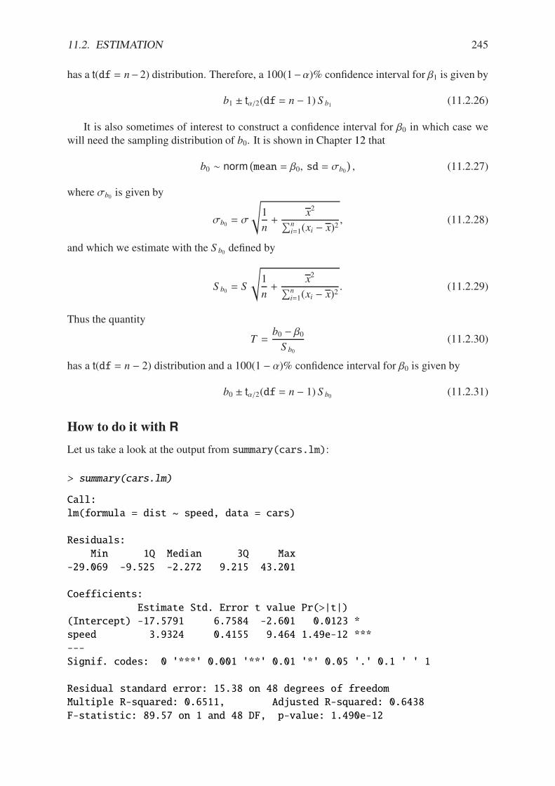
11.2. ESTIMATION 245
has a t(df = n#2) distribution. Therefore, a 100(1#()% confidence interval for *1 is given by
b1 ± t(/2(df = n # 1) S b1 (11.2.26)
It is also sometimes of interest to construct a confidence interval for *0 in which case wewill need the sampling distribution of b0. It is shown in Chapter 12 that
b0 4 norm=mean = *0, sd = "b0
>, (11.2.27)
where "b0 is given by
"b0 = "
X1
n+
x2#n
i=1(xi # x)2, (11.2.28)
and which we estimate with the S b0 defined by
S b0 = S
X1
n+
x2#n
i=1(xi # x)2. (11.2.29)
Thus the quantity
T =b0 # *0S b0
(11.2.30)
has a t(df = n # 2) distribution and a 100(1 # ()% confidence interval for *0 is given by
b0 ± t(/2(df = n # 1) S b0 (11.2.31)
How to do it with R
Let us take a look at the output from summary(cars.lm):
> summary(cars.lm)
Call:
lm(formula = dist ~ speed, data = cars)
Residuals:
Min 1Q Median 3Q Max
-29.069 -9.525 -2.272 9.215 43.201
Coefficients:
Estimate Std. Error t value Pr(>|t|)
(Intercept) -17.5791 6.7584 -2.601 0.0123 *
speed 3.9324 0.4155 9.464 1.49e-12 ***
---
Signif. codes: 0 '***' 0.001 '**' 0.01 '*' 0.05 '.' 0.1 ' ' 1
Residual standard error: 15.38 on 48 degrees of freedom
Multiple R-squared: 0.6511, Adjusted R-squared: 0.6438
F-statistic: 89.57 on 1 and 48 DF, p-value: 1.490e-12
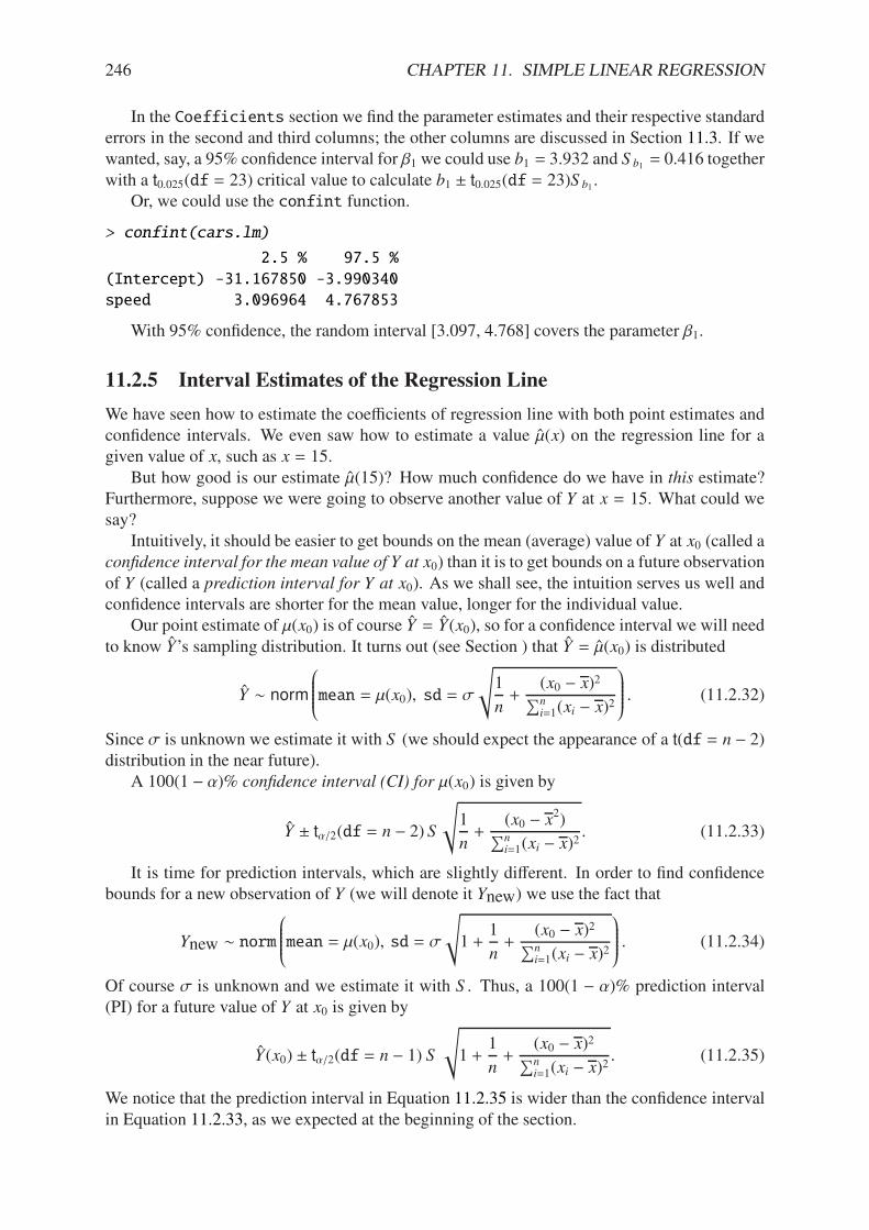
246 CHAPTER 11. SIMPLE LINEAR REGRESSION
In the Coefficients section we find the parameter estimates and their respective standarderrors in the second and third columns; the other columns are discussed in Section 11.3. If wewanted, say, a 95% confidence interval for *1 we could use b1 = 3.932 and S b1 = 0.416 togetherwith a t0.025(df = 23) critical value to calculate b1 ± t0.025(df = 23)S b1 .
Or, we could use the confint function.
> confint(cars.lm)
2.5 % 97.5 %
(Intercept) -31.167850 -3.990340
speed 3.096964 4.767853
With 95% confidence, the random interval [3.097, 4.768] covers the parameter *1.
11.2.5 Interval Estimates of the Regression Line
We have seen how to estimate the coe"cients of regression line with both point estimates andconfidence intervals. We even saw how to estimate a value µ(x) on the regression line for agiven value of x, such as x = 15.
But how good is our estimate µ(15)? How much confidence do we have in this estimate?Furthermore, suppose we were going to observe another value of Y at x = 15. What could wesay?
Intuitively, it should be easier to get bounds on the mean (average) value of Y at x0 (called aconfidence interval for the mean value of Y at x0) than it is to get bounds on a future observationof Y (called a prediction interval for Y at x0). As we shall see, the intuition serves us well andconfidence intervals are shorter for the mean value, longer for the individual value.
Our point estimate of µ(x0) is of course Y = Y(x0), so for a confidence interval we will needto know Y’s sampling distribution. It turns out (see Section ) that Y = µ(x0) is distributed
Y 4 norm
$%%%%%%&mean = µ(x0), sd = "
X1
n+
(x0 # x)2#n
i=1(xi # x)2
())))))* . (11.2.32)
Since " is unknown we estimate it with S (we should expect the appearance of a t(df = n # 2)distribution in the near future).
A 100(1 # ()% confidence interval (CI) for µ(x0) is given by
Y ± t(/2(df = n # 2) S
X1
n+
(x0 # x2)#n
i=1(xi # x)2. (11.2.33)
It is time for prediction intervals, which are slightly di!erent. In order to find confidencebounds for a new observation of Y (we will denote it Ynew) we use the fact that
Ynew 4 norm
$%%%%%%&mean = µ(x0), sd = "
X
1 +1
n+
(x0 # x)2#n
i=1(xi # x)2
())))))* . (11.2.34)
Of course " is unknown and we estimate it with S . Thus, a 100(1 # ()% prediction interval(PI) for a future value of Y at x0 is given by
Y(x0) ± t(/2(df = n # 1) S
X
1 +1
n+
(x0 # x)2#n
i=1(xi # x)2. (11.2.35)
We notice that the prediction interval in Equation 11.2.35 is wider than the confidence intervalin Equation 11.2.33, as we expected at the beginning of the section.
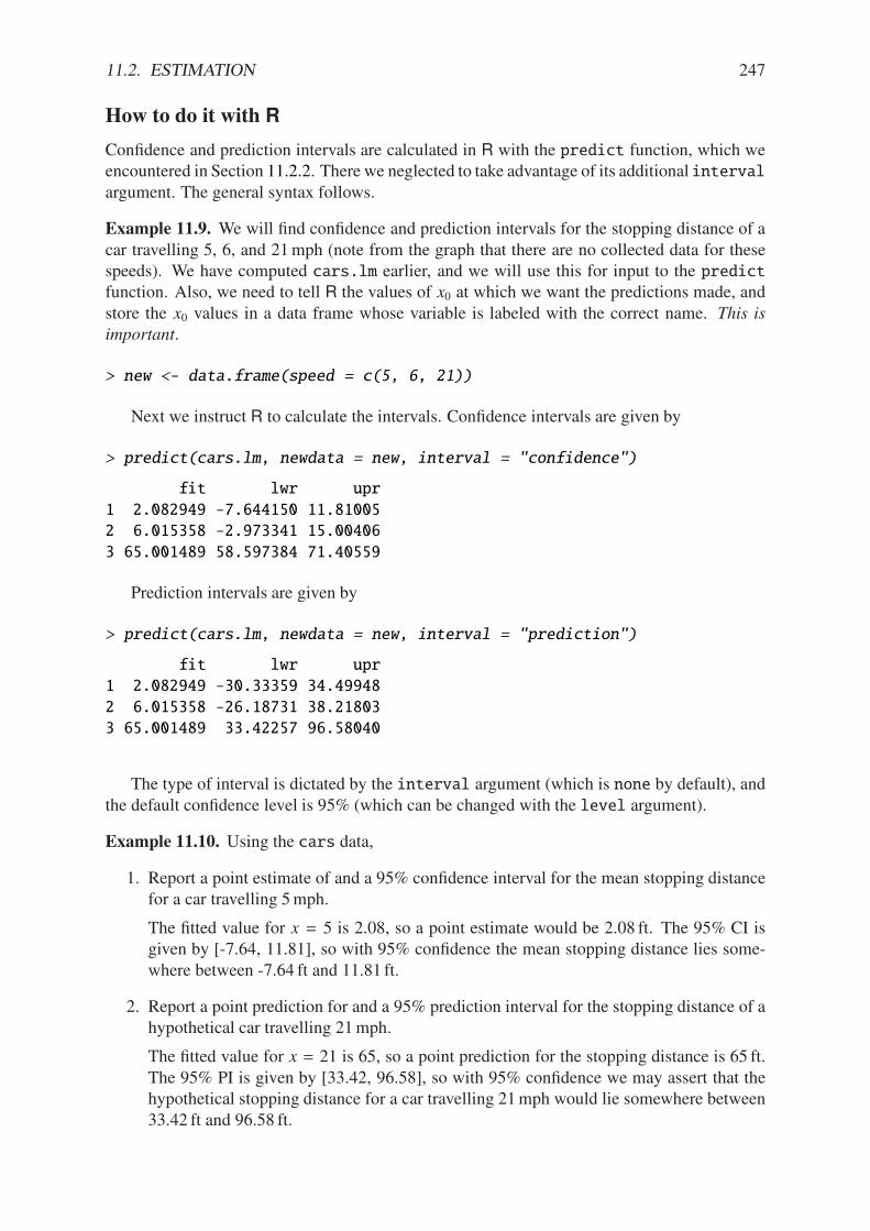
11.2. ESTIMATION 247
How to do it with R
Confidence and prediction intervals are calculated in R with the predict function, which weencountered in Section 11.2.2. There we neglected to take advantage of its additional intervalargument. The general syntax follows.
Example 11.9. We will find confidence and prediction intervals for the stopping distance of acar travelling 5, 6, and 21mph (note from the graph that there are no collected data for thesespeeds). We have computed cars.lm earlier, and we will use this for input to the predictfunction. Also, we need to tell R the values of x0 at which we want the predictions made, andstore the x0 values in a data frame whose variable is labeled with the correct name. This is
important.
> new <- data.frame(speed = c(5, 6, 21))
Next we instruct R to calculate the intervals. Confidence intervals are given by
> predict(cars.lm, newdata = new, interval = "confidence")
fit lwr upr
1 2.082949 -7.644150 11.81005
2 6.015358 -2.973341 15.00406
3 65.001489 58.597384 71.40559
Prediction intervals are given by
> predict(cars.lm, newdata = new, interval = "prediction")
fit lwr upr
1 2.082949 -30.33359 34.49948
2 6.015358 -26.18731 38.21803
3 65.001489 33.42257 96.58040
The type of interval is dictated by the interval argument (which is none by default), andthe default confidence level is 95% (which can be changed with the level argument).
Example 11.10. Using the cars data,
1. Report a point estimate of and a 95% confidence interval for the mean stopping distancefor a car travelling 5mph.
The fitted value for x = 5 is 2.08, so a point estimate would be 2.08 ft. The 95% CI isgiven by [-7.64, 11.81], so with 95% confidence the mean stopping distance lies some-where between -7.64 ft and 11.81 ft.
2. Report a point prediction for and a 95% prediction interval for the stopping distance of ahypothetical car travelling 21mph.
The fitted value for x = 21 is 65, so a point prediction for the stopping distance is 65 ft.The 95% PI is given by [33.42, 96.58], so with 95% confidence we may assert that thehypothetical stopping distance for a car travelling 21mph would lie somewhere between33.42 ft and 96.58 ft.
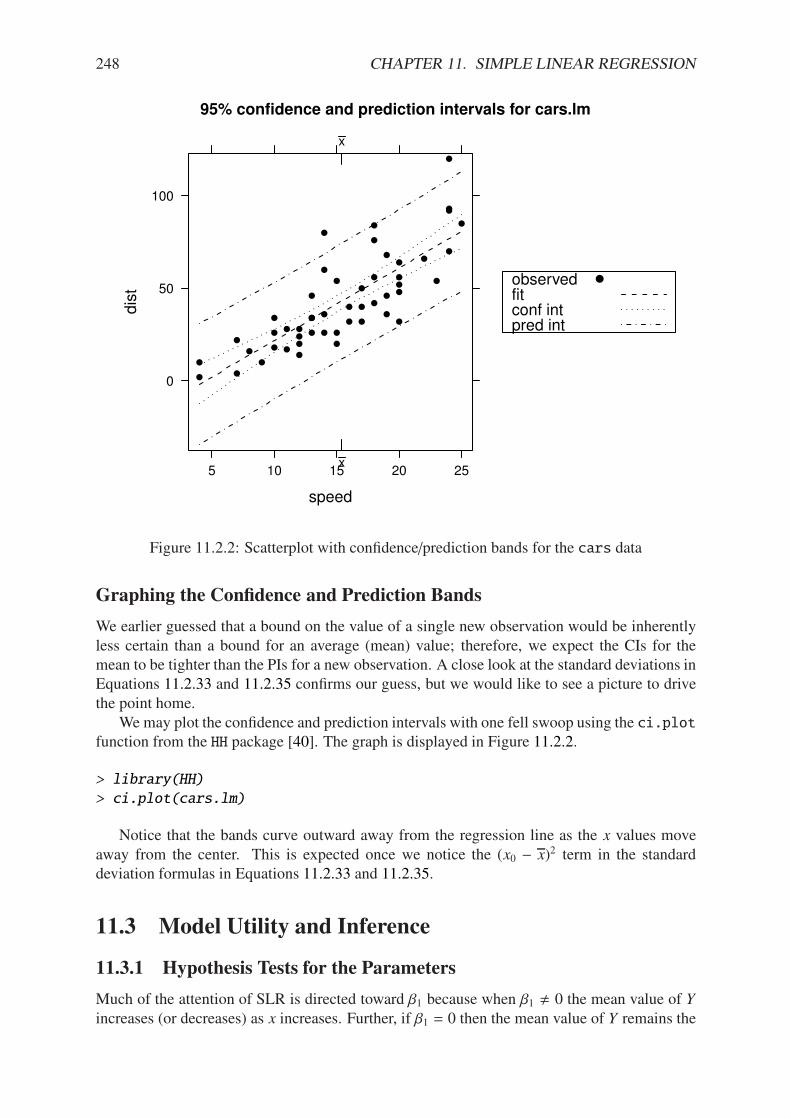
248 CHAPTER 11. SIMPLE LINEAR REGRESSION
95% confidence and prediction intervals for cars.lm
speed
dis
t
0
50
100
5 10 15 20 25x
x
observedfitconf intpred int
Figure 11.2.2: Scatterplot with confidence/prediction bands for the cars data
Graphing the Confidence and Prediction Bands
We earlier guessed that a bound on the value of a single new observation would be inherentlyless certain than a bound for an average (mean) value; therefore, we expect the CIs for themean to be tighter than the PIs for a new observation. A close look at the standard deviations inEquations 11.2.33 and 11.2.35 confirms our guess, but we would like to see a picture to drivethe point home.
We may plot the confidence and prediction intervals with one fell swoop using the ci.plotfunction from the HH package [40]. The graph is displayed in Figure 11.2.2.
> library(HH)
> ci.plot(cars.lm)
Notice that the bands curve outward away from the regression line as the x values moveaway from the center. This is expected once we notice the (x0 # x)2 term in the standarddeviation formulas in Equations 11.2.33 and 11.2.35.
11.3 Model Utility and Inference
11.3.1 Hypothesis Tests for the Parameters
Much of the attention of SLR is directed toward *1 because when *1 ! 0 the mean value of Yincreases (or decreases) as x increases. Further, if *1 = 0 then the mean value of Y remains the
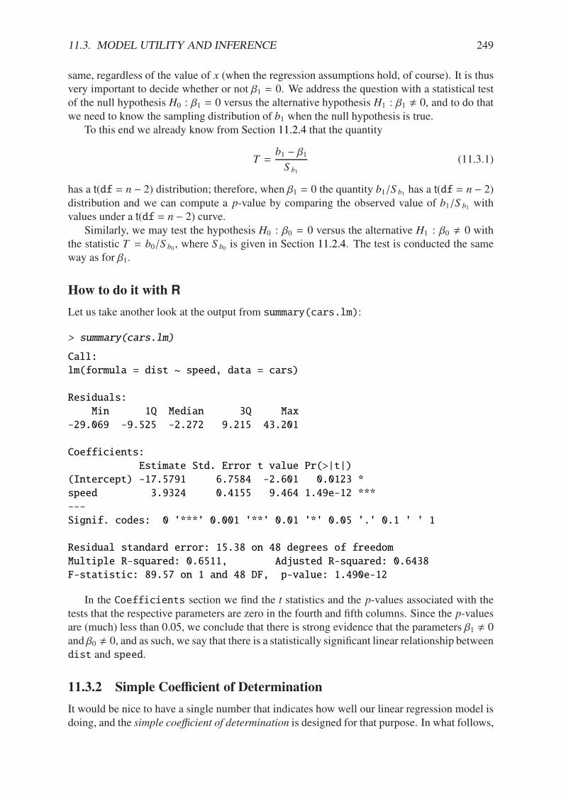
11.3. MODEL UTILITY AND INFERENCE 249
same, regardless of the value of x (when the regression assumptions hold, of course). It is thusvery important to decide whether or not *1 = 0. We address the question with a statistical testof the null hypothesis H0 : *1 = 0 versus the alternative hypothesis H1 : *1 ! 0, and to do thatwe need to know the sampling distribution of b1 when the null hypothesis is true.
To this end we already know from Section 11.2.4 that the quantity
T =b1 # *1S b1
(11.3.1)
has a t(df = n # 2) distribution; therefore, when *1 = 0 the quantity b1/S b1 has a t(df = n # 2)distribution and we can compute a p-value by comparing the observed value of b1/S b1 withvalues under a t(df = n # 2) curve.
Similarly, we may test the hypothesis H0 : *0 = 0 versus the alternative H1 : *0 ! 0 withthe statistic T = b0/S b0 , where S b0 is given in Section 11.2.4. The test is conducted the sameway as for *1.
How to do it with R
Let us take another look at the output from summary(cars.lm):
> summary(cars.lm)
Call:
lm(formula = dist ~ speed, data = cars)
Residuals:
Min 1Q Median 3Q Max
-29.069 -9.525 -2.272 9.215 43.201
Coefficients:
Estimate Std. Error t value Pr(>|t|)
(Intercept) -17.5791 6.7584 -2.601 0.0123 *
speed 3.9324 0.4155 9.464 1.49e-12 ***
---
Signif. codes: 0 '***' 0.001 '**' 0.01 '*' 0.05 '.' 0.1 ' ' 1
Residual standard error: 15.38 on 48 degrees of freedom
Multiple R-squared: 0.6511, Adjusted R-squared: 0.6438
F-statistic: 89.57 on 1 and 48 DF, p-value: 1.490e-12
In the Coefficients section we find the t statistics and the p-values associated with thetests that the respective parameters are zero in the fourth and fifth columns. Since the p-valuesare (much) less than 0.05, we conclude that there is strong evidence that the parameters *1 ! 0and *0 ! 0, and as such, we say that there is a statistically significant linear relationship betweendist and speed.
11.3.2 Simple Coe"cient of Determination
It would be nice to have a single number that indicates how well our linear regression model isdoing, and the simple coe!cient of determination is designed for that purpose. In what follows,
250 CHAPTER 11. SIMPLE LINEAR REGRESSION
we observe the values Y1, Y2, . . . ,Yn, and the goal is to estimate µ(x0), the mean value of Y atthe location x0.
If we disregard the dependence of Y and x and base our estimate only on the Y values thena reasonable choice for an estimator is just the MLE of µ, which is Y . Then the errors incurredby the estimate are just Yi # Y and the variation about the estimate as measured by the samplevariance is proportional to
S S TO =
n!
i=1
(Yi # Y)2. (11.3.2)
Here, S S TO is an acronym for the total sum of squares.But we do have additional information, namely, we have values xi associated with each
value of Yi. We have seen that this information leads us to the estimate Yi and the errorsincurred are just the residuals, Ei = Yi # Yi. The variation associated with these errors can bemeasured with
S S E =
n!
i=1
(Yi # Yi)2. (11.3.3)
We have seen the S S E before, which stands for the sum of squared errors or error sum of
squares. Of course, we would expect the error to be less in the latter case, since we have usedmore information. The improvement in our estimation as a result of the linear regression modelcan be measured with the di!erence
(Yi # Y) # (Yi # Yi) = Yi # Y ,
and we measure the variation in these errors with
S SR =
n!
i=1
(Yi # Y)2, (11.3.4)
also known as the regression sum of squares. It is not obvious, but some algebra proved afamous result known as the ANOVA Equality:
n!
i=1
(Yi # Y)2 =n!
i=1
(Yi # Y)2 +n!
i=1
(Yi # Yi)2 (11.3.5)
or in other words,S S TO = S SR + S S E. (11.3.6)
This equality has a nice interpretation. Consider S S TO to be the total variation of the errors.Think of a decomposition of the total variation into pieces: one piece measuring the reductionof error from using the linear regression model, or explained variation (S SR), while the otherrepresents what is left over, that is, the errors that the linear regression model doesn’t explain,or unexplained variation (S S E). In this way we see that the ANOVA equality merely partitionsthe variation into
total variation = explained variation + unexplained variation.
For a single number to summarize how well our model is doing we use the simple coe"cientof determination r2, defined by
r2 = 1 #S S E
S S TO. (11.3.7)
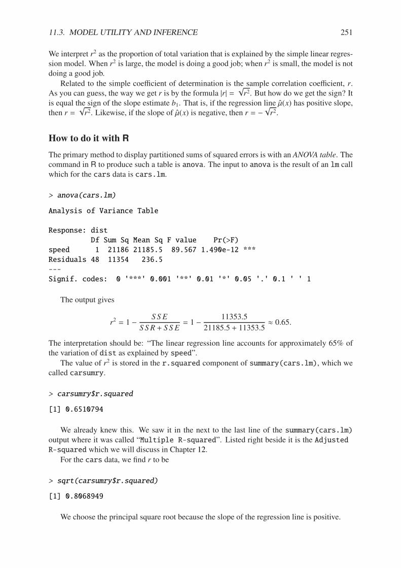
11.3. MODEL UTILITY AND INFERENCE 251
We interpret r2 as the proportion of total variation that is explained by the simple linear regres-sion model. When r2 is large, the model is doing a good job; when r2 is small, the model is notdoing a good job.
Related to the simple coe"cient of determination is the sample correlation coe"cient, r.As you can guess, the way we get r is by the formula |r| =
$r2. But how do we get the sign? It
is equal the sign of the slope estimate b1. That is, if the regression line µ(x) has positive slope,then r =
$r2. Likewise, if the slope of µ(x) is negative, then r = #
$r2.
How to do it with R
The primary method to display partitioned sums of squared errors is with an ANOVA table. Thecommand in R to produce such a table is anova. The input to anova is the result of an lm callwhich for the cars data is cars.lm.
> anova(cars.lm)
Analysis of Variance Table
Response: dist
Df Sum Sq Mean Sq F value Pr(>F)
speed 1 21186 21185.5 89.567 1.490e-12 ***
Residuals 48 11354 236.5
---
Signif. codes: 0 '***' 0.001 '**' 0.01 '*' 0.05 '.' 0.1 ' ' 1
The output gives
r2 = 1 #S S E
S SR + S S E= 1 #
11353.5
21185.5 + 11353.5' 0.65.
The interpretation should be: “The linear regression line accounts for approximately 65% ofthe variation of dist as explained by speed”.
The value of r2 is stored in the r.squared component of summary(cars.lm), which wecalled carsumry.
> carsumry$r.squared
[1] 0.6510794
We already knew this. We saw it in the next to the last line of the summary(cars.lm)output where it was called “Multiple R-squared”. Listed right beside it is the AdjustedR-squared which we will discuss in Chapter 12.
For the cars data, we find r to be
> sqrt(carsumry$r.squared)
[1] 0.8068949
We choose the principal square root because the slope of the regression line is positive.
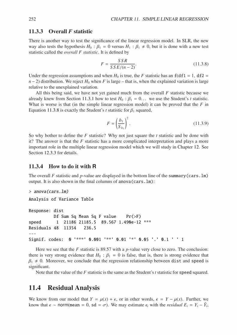
252 CHAPTER 11. SIMPLE LINEAR REGRESSION
11.3.3 Overall F statistic
There is another way to test the significance of the linear regression model. In SLR, the newway also tests the hypothesis H0 : *1 = 0 versus H1 : *1 ! 0, but it is done with a new teststatistic called the overall F statistic. It is defined by
F =S SR
S S E/(n # 2). (11.3.8)
Under the regression assumptions and when H0 is true, the F statistic has an f(df1 = 1, df2 =n# 2) distribution. We reject H0 when F is large – that is, when the explained variation is largerelative to the unexplained variation.
All this being said, we have not yet gained much from the overall F statistic because wealready knew from Section 11.3.1 how to test H0 : *1 = 0. . . we use the Student’s t statistic.What is worse is that (in the simple linear regression model) it can be proved that the F inEquation 11.3.8 is exactly the Student’s t statistic for *1 squared,
F =
0b1
S b1
12. (11.3.9)
So why bother to define the F statistic? Why not just square the t statistic and be done withit? The answer is that the F statistic has a more complicated interpretation and plays a moreimportant role in the multiple linear regression model which we will study in Chapter 12. SeeSection 12.3.3 for details.
11.3.4 How to do it with R
The overall F statistic and p-value are displayed in the bottom line of the summary(cars.lm)output. It is also shown in the final columns of anova(cars.lm):
> anova(cars.lm)
Analysis of Variance Table
Response: dist
Df Sum Sq Mean Sq F value Pr(>F)
speed 1 21186 21185.5 89.567 1.490e-12 ***
Residuals 48 11354 236.5
---
Signif. codes: 0 '***' 0.001 '**' 0.01 '*' 0.05 '.' 0.1 ' ' 1
Here we see that the F statistic is 89.57 with a p-value very close to zero. The conclusion:there is very strong evidence that H0 : *1 = 0 is false, that is, there is strong evidence that*1 ! 0. Moreover, we conclude that the regression relationship between dist and speed issignificant.
Note that the value of the F statistic is the same as the Student’s t statistic for speed squared.
11.4 Residual Analysis
We know from our model that Y = µ(x) + $, or in other words, $ = Y # µ(x). Further, weknow that $ 4 norm(mean = 0, sd = "). We may estimate $i with the residual Ei = Yi # Yi,
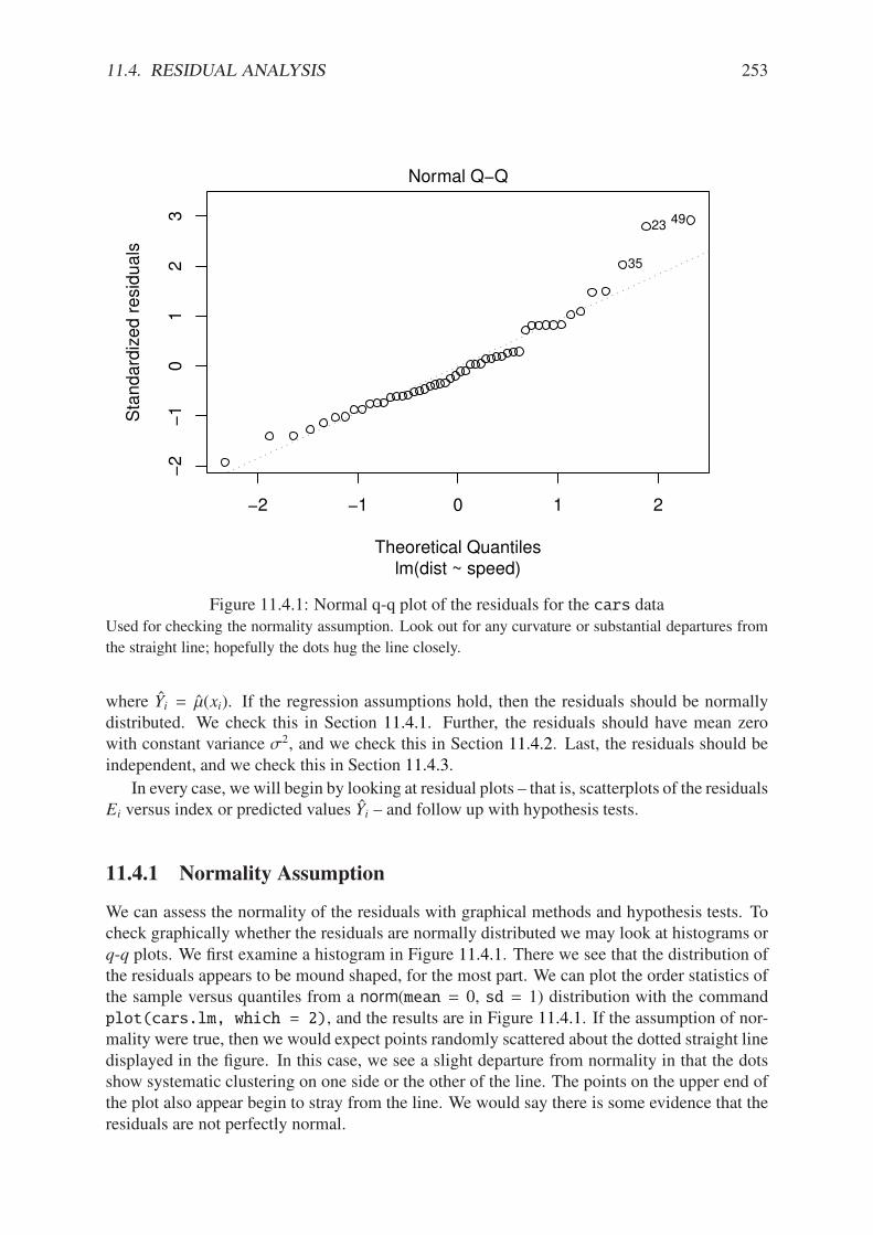
11.4. RESIDUAL ANALYSIS 253
!2 !1 0 1 2
!2
!1
01
23
Theoretical Quantiles
Sta
ndard
ized r
esi
duals
lm(dist ~ speed)
Normal Q!Q
4923
35
Figure 11.4.1: Normal q-q plot of the residuals for the cars dataUsed for checking the normality assumption. Look out for any curvature or substantial departures from
the straight line; hopefully the dots hug the line closely.
where Yi = µ(xi). If the regression assumptions hold, then the residuals should be normallydistributed. We check this in Section 11.4.1. Further, the residuals should have mean zerowith constant variance "2, and we check this in Section 11.4.2. Last, the residuals should beindependent, and we check this in Section 11.4.3.
In every case, we will begin by looking at residual plots – that is, scatterplots of the residualsEi versus index or predicted values Yi – and follow up with hypothesis tests.
11.4.1 Normality Assumption
We can assess the normality of the residuals with graphical methods and hypothesis tests. Tocheck graphically whether the residuals are normally distributed we may look at histograms orq-q plots. We first examine a histogram in Figure 11.4.1. There we see that the distribution ofthe residuals appears to be mound shaped, for the most part. We can plot the order statistics ofthe sample versus quantiles from a norm(mean = 0, sd = 1) distribution with the commandplot(cars.lm, which = 2), and the results are in Figure 11.4.1. If the assumption of nor-mality were true, then we would expect points randomly scattered about the dotted straight linedisplayed in the figure. In this case, we see a slight departure from normality in that the dotsshow systematic clustering on one side or the other of the line. The points on the upper end ofthe plot also appear begin to stray from the line. We would say there is some evidence that theresiduals are not perfectly normal.
254 CHAPTER 11. SIMPLE LINEAR REGRESSION
Testing the Normality Assumption
Even though we may be concerned about the plots, we can use tests to determine if the evidencepresent is statistically significant, or if it could have happened merely by chance. There aremany statistical tests of normality. We will use the Shapiro-Wilk test, since it is known to bea good test and to be quite powerful. However, there are many other fine tests of normalityincluding the Anderson-Darling test and the Lillefors test, just to mention two of them.
The Shapiro-Wilk test is based on the statistic
W =
=#ni=1 aiE(i)
>2#n
j=1 E2j
, (11.4.1)
where the E(i) are the ordered residuals and the ai are constants derived from the order statisticsof a sample of size n from a normal distribution. See Section 10.5.3.
We perform the Shapiro-Wilk test below, using the shapiro.test function from the statspackage. The hypotheses are
H0 : the residuals are normally distributed
versusH1 : the residuals are not normally distributed.
The results from R are
> shapiro.test(residuals(cars.lm))
Shapiro-Wilk normality test
data: residuals(cars.lm)
W = 0.9451, p-value = 0.02153
For these data we would reject the assumption of normality of the residuals at the ( = 0.05significance level, but do not lose heart, because the regression model is reasonably robust todepartures from the normality assumption. As long as the residual distribution is not highlyskewed, then the regression estimators will perform reasonably well. Moreover, departuresfrom constant variance and independence will sometimes a!ect the quantile plots and his-tograms, therefore it is wise to delay final decisions regarding normality until all diagnosticmeasures have been investigated.
11.4.2 Constant Variance Assumption
We will again go to residual plots to try and determine if the spread of the residuals is changingover time (or index). However, it is unfortunately not that easy because the residuals do nothave constant variance! In fact, it can be shown that the variance of the residual Ei is
Var(Ei) = "2(1 # hii), i = 1, 2, . . . , n, (11.4.2)
where hii is a quantity called the leverage which is defined below. Consequently, in order tocheck the constant variance assumption we must standardize the residuals before plotting. Weestimate the standard error of Ei with sEi
= s$(1 # hii) and define the standardized residuals
Ri, i = 1, 2, . . . , n, by
Ri =Ei
s$1 # hii
, i = 1, 2, . . . , n. (11.4.3)
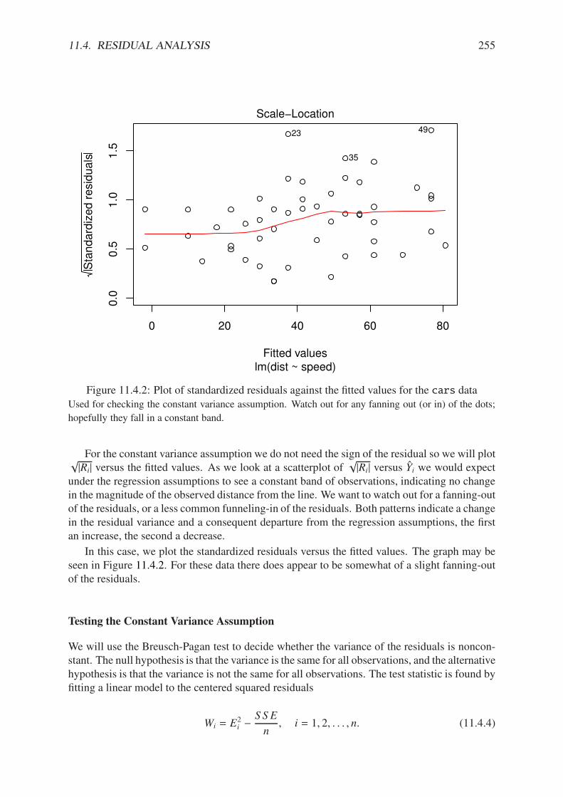
11.4. RESIDUAL ANALYSIS 255
0 20 40 60 80
0.0
0.5
1.0
1.5
Fitted values
Sta
ndard
ized
resi
duals
lm(dist ~ speed)
Scale!Location
4923
35
Figure 11.4.2: Plot of standardized residuals against the fitted values for the cars dataUsed for checking the constant variance assumption. Watch out for any fanning out (or in) of the dots;
hopefully they fall in a constant band.
For the constant variance assumption we do not need the sign of the residual so we will plot$|Ri| versus the fitted values. As we look at a scatterplot of
$|Ri| versus Yi we would expect
under the regression assumptions to see a constant band of observations, indicating no changein the magnitude of the observed distance from the line. We want to watch out for a fanning-outof the residuals, or a less common funneling-in of the residuals. Both patterns indicate a changein the residual variance and a consequent departure from the regression assumptions, the firstan increase, the second a decrease.
In this case, we plot the standardized residuals versus the fitted values. The graph may beseen in Figure 11.4.2. For these data there does appear to be somewhat of a slight fanning-outof the residuals.
Testing the Constant Variance Assumption
We will use the Breusch-Pagan test to decide whether the variance of the residuals is noncon-stant. The null hypothesis is that the variance is the same for all observations, and the alternativehypothesis is that the variance is not the same for all observations. The test statistic is found byfitting a linear model to the centered squared residuals
Wi = E2i #
S S E
n, i = 1, 2, . . . , n. (11.4.4)
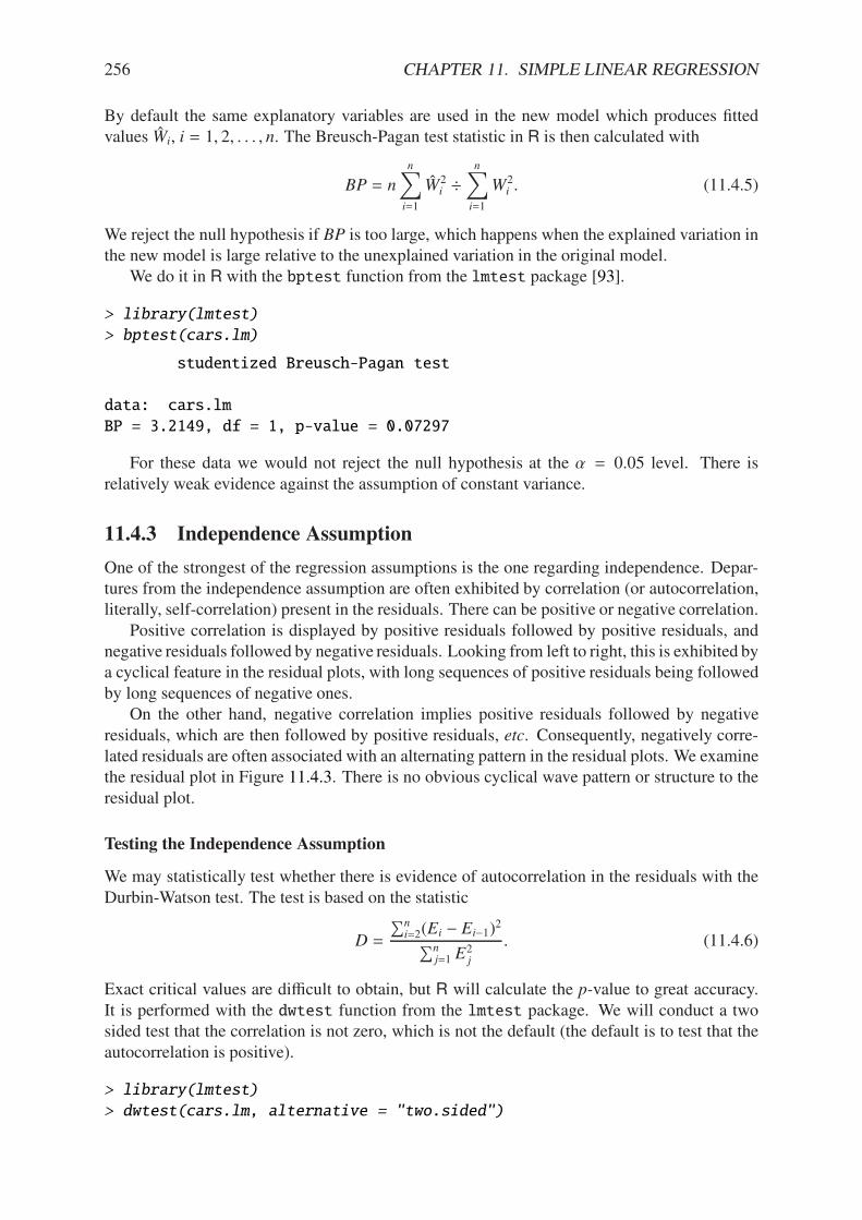
256 CHAPTER 11. SIMPLE LINEAR REGRESSION
By default the same explanatory variables are used in the new model which produces fittedvalues Wi, i = 1, 2, . . . , n. The Breusch-Pagan test statistic in R is then calculated with
BP = n
n!
i=1
W2i ÷
n!
i=1
W2i . (11.4.5)
We reject the null hypothesis if BP is too large, which happens when the explained variation inthe new model is large relative to the unexplained variation in the original model.
We do it in R with the bptest function from the lmtest package [93].
> library(lmtest)
> bptest(cars.lm)
studentized Breusch-Pagan test
data: cars.lm
BP = 3.2149, df = 1, p-value = 0.07297
For these data we would not reject the null hypothesis at the ( = 0.05 level. There isrelatively weak evidence against the assumption of constant variance.
11.4.3 Independence Assumption
One of the strongest of the regression assumptions is the one regarding independence. Depar-tures from the independence assumption are often exhibited by correlation (or autocorrelation,literally, self-correlation) present in the residuals. There can be positive or negative correlation.
Positive correlation is displayed by positive residuals followed by positive residuals, andnegative residuals followed by negative residuals. Looking from left to right, this is exhibited bya cyclical feature in the residual plots, with long sequences of positive residuals being followedby long sequences of negative ones.
On the other hand, negative correlation implies positive residuals followed by negativeresiduals, which are then followed by positive residuals, etc. Consequently, negatively corre-lated residuals are often associated with an alternating pattern in the residual plots. We examinethe residual plot in Figure 11.4.3. There is no obvious cyclical wave pattern or structure to theresidual plot.
Testing the Independence Assumption
We may statistically test whether there is evidence of autocorrelation in the residuals with theDurbin-Watson test. The test is based on the statistic
D =
#ni=2(Ei # Ei#1)
2
#nj=1 E
2j
. (11.4.6)
Exact critical values are di"cult to obtain, but R will calculate the p-value to great accuracy.It is performed with the dwtest function from the lmtest package. We will conduct a twosided test that the correlation is not zero, which is not the default (the default is to test that theautocorrelation is positive).
> library(lmtest)
> dwtest(cars.lm, alternative = "two.sided")
11.4. RESIDUAL ANALYSIS 257
0 20 40 60 80
!20
020
40
Fitted values
Resi
duals
lm(dist ~ speed)
Residuals vs Fitted
4923
35
Figure 11.4.3: Plot of the residuals versus the fitted values for the cars dataUsed for checking the independence assumption. Watch out for any patterns or structure; hopefully the
points are randomly scattered on the plot.
258 CHAPTER 11. SIMPLE LINEAR REGRESSION
Durbin-Watson test
data: cars.lm
DW = 1.6762, p-value = 0.1904
alternative hypothesis: true autocorelation is not 0
In this case we do not reject the null hypothesis at the ( = 0.05 significance level; there isvery little evidence of nonzero autocorrelation in the residuals.
11.4.4 Remedial Measures
We often find problems with our model that suggest that at least one of the three regressionassumptions is violated. What do we do then? There are many measures at the statistician’sdisposal, and we mention specific steps one can take to improve the model under certain typesof violation.
Mean response is not linear. We can directly modify the model to better approximate themean response. In particular, perhaps a polynomial regression function of the form
µ(x) = *0 + *1x1 + *2x21
would be appropriate. Alternatively, we could have a function of the form
µ(x) = *0e*1x.
Models like these are studied in nonlinear regression courses.
Error variance is not constant. Sometimes a transformation of the dependent variable willtake care of the problem. There is a large class of them called Box-Cox transformations.They take the form
Y6 = Y%, (11.4.7)
where % is a constant. (The method proposed by Box and Cox will determine a suitablevalue of % automatically by maximum likelihood). The class contains the transformations
% = 2, Y6 = Y2
% = 0.5, Y6 =$Y
% = 0, Y6 = ln Y
% = #1, Y6 = 1/Y
Alternatively, we can use the method of weighted least squares. This is studied in moredetail in later classes.
Error distribution is not normal. The same transformations for stabilizing the variance areequally appropriate for smoothing the residuals to a more Gaussian form. In fact, oftenwe will kill two birds with one stone.
Errors are not independent. There is a large class of autoregressive models to be used in thissituation which occupy the latter part of Chapter 16.
11.5. OTHER DIAGNOSTIC TOOLS 259
11.5 Other Diagnostic Tools
There are two types of observations with which we must be especially careful:
Influential observations are those that have a substantial e!ect on our estimates, predictions,or inferences. A small change in an influential observation is followed by a large changein the parameter estimates or inferences.
Outlying observations are those that fall fall far from the rest of the data. They may be indicat-ing a lack of fit for our regression model, or they may just be a mistake or typographicalerror that should be corrected. Regardless, special attention should be given to theseobservations. An outlying observation may or may not be influential.
We will discuss outliers first because the notation builds sequentially in that order.
11.5.1 Outliers
There are three ways that an observation (xi, yi) may be an outlier: it can have an xi value whichfalls far from the other x values, it can have a yi value which falls far from the other y values,or it can have both its xi and yi values falling far from the other x and y values.
Leverage
Leverage statistics are designed to identify observations which have x values that are far awayfrom the rest of the data. In the simple linear regression model the leverage of xi is denoted byhii and defined by
hii =1
n+
(xi # x)2#n
k=1(xk # x)2, i = 1, 2, . . . , n. (11.5.1)
The formula has a nice interpretation in the SLR model: if the distance from xi to x is largerelative to the other x’s then hii will be close to 1.
Leverages have nice mathematical properties; for example, they satisfy
0 " hii " 1, (11.5.2)
and their sum is
n!
i=1
hii =
n!
i=1
71
n+
(xi # x)2#n
k=1(xk # x)2
8, (11.5.3)
=n
n+
#i(xi # x)2
#k(xk # x)2
, (11.5.4)
= 2. (11.5.5)
A rule of thumb is to consider leverage values to be large if they are more than double theiraverage size (which is 2/n according to Equation 11.5.5). So leverages larger than 4/n aresuspect. Another rule of thumb is to say that values bigger than 0.5 indicate high leverage,while values between 0.3 and 0.5 indicate moderate leverage.
260 CHAPTER 11. SIMPLE LINEAR REGRESSION
Standardized and Studentized Deleted Residuals
We have already encountered the standardized residuals ri in Section 11.4.2; they are merelyresiduals that have been divided by their respective standard deviations:
Ri =Ei
S$1 # hii
, i = 1, 2, . . . , n. (11.5.6)
Values of |Ri| > 2 are extreme and suggest that the observation has an outlying y-value.Now delete the ith case and fit the regression function to the remaining n#1 cases, producing
a fitted value Y(i) with deleted residual Di = Yi # Y(i). It is shown in later classes that
Var(Di) =S 2(i)
1 # hii, i = 1, 2, . . . , n, (11.5.7)
so that the studentized deleted residuals ti defined by
ti =Di
S (i)/(1 # hii), i = 1, 2, . . . , n, (11.5.8)
have a t(df = n # 3) distribution and we compare observed values of ti to this distribution todecide whether or not an observation is extreme.
The folklore in regression classes is that a test based on the statistic in Equation 11.5.8 canbe too liberal. A rule of thumb is if we suspect an observation to be an outlier before seeingthe data then we say it is significantly outlying if its two-tailed p-value is less than (, but ifwe suspect an observation to be an outlier after seeing the data then we should only say it issignificantly outlying if its two-tailed p-value is less than (/n. The latter rule of thumb is calledthe Bonferroni approach and can be overly conservative for large data sets. The responsiblestatistician should look at the data and use his/her best judgement, in every case.
11.5.2 How to do it with R
We can calculate the standardized residuals with the rstandard function. The input is the lmobject, which is cars.lm.
> sres <- rstandard(cars.lm)
> sres[1:5]
1 2 3 4 5
0.2660415 0.8189327 -0.4013462 0.8132663 0.1421624
We can find out which observations have studentized residuals larger than two with thecommand
> sres[which(abs(sres) > 2)]
23 35 49
2.795166 2.027818 2.919060
In this case, we see that observations 23, 35, and 49 are potential outliers with respect totheir y-value.
We can compute the studentized deleted residuals with rstudent:
11.5. OTHER DIAGNOSTIC TOOLS 261
> sdelres <- rstudent(cars.lm)
> sdelres[1:5]
1 2 3 4 5
0.2634500 0.8160784 -0.3978115 0.8103526 0.1407033
We should compare these values with critical values from a t(df = n#3) distribution, whichin this case is t(df = 50 # 3 = 47). We can calculate a 0.005 quantile and check with
> t0.005 <- qt(0.005, df = 47, lower.tail = FALSE)
> sdelres[which(abs(sdelres) > t0.005)]
23 49
3.022829 3.184993
This means that observations 23 and 49 have a large studentized deleted residual. Theleverages can be found with the hatvalues function:
> leverage <- hatvalues(cars.lm)
> leverage[1:5]
1 2 3 4 5
0.11486131 0.11486131 0.07150365 0.07150365 0.05997080
> leverage[which(leverage > 4/50)]
1 2 50
0.11486131 0.11486131 0.08727007
Here we see that observations 1, 2, and 50 have leverages bigger than double their meanvalue. These observations would be considered outlying with respect to their x value (althoughthey may or may not be influential).
11.5.3 Influential Observations
DFBETAS and DFFITS
Anytime we do a statistical analysis, we are confronted with the variability of data. It is alwaysa concern when an observation plays too large a role in our regression model, and we wouldnot like or procedures to be overly influenced by the value of a single observation. Hence,it becomes desirable to check to see how much our estimates and predictions would changeif one of the observations were not included in the analysis. If an observation changes theestimates/predictions a large amount, then the observation is influential and should be subjectedto a higher level of scrutiny.
We measure the change in the parameter estimates as a result of deleting an observationwith DFBETAS . The DFBETAS for the intercept b0 are given by
(DFBETAS )0(i) =b0 # b0(i)
S (i)
M1n+ x2#n
i=1(xi#x)2
, i = 1, 2, . . . , n. (11.5.9)
and the DFBETAS for the slope b1 are given by
(DFBETAS )1(i) =b1 # b1(i)
S (i)
R#ni=1(xi # x)2
S#1/2 , i = 1, 2, . . . , n. (11.5.10)
262 CHAPTER 11. SIMPLE LINEAR REGRESSION
See Section 12.8 for a better way to write these. The signs of the DFBETAS indicate whetherthe coe"cients would increase or decrease as a result of including the observation. If theDFBETAS are large, then the observation has a large impact on those regression coe"cients.We label observations as suspicious if theirDFBETAS have magnitude greater 1 for small dataor 2/
$n for large data sets.
We can calculate the DFBETAS with the dfbetas function (some output has been omit-ted):
> dfb <- dfbetas(cars.lm)
> head(dfb)
(Intercept) speed
1 0.09440188 -0.08624563
2 0.29242487 -0.26715961
3 -0.10749794 0.09369281
4 0.21897614 -0.19085472
5 0.03407516 -0.02901384
6 -0.11100703 0.09174024
We see that the inclusion of the first observation slightly increases the Intercept andslightly decreases the coe"cient on speed.
We can measure the influence that an observation has on its fitted value with DFFITS .These are calculated by deleting an observation, refitting the model, recalculating the fit, thenstandardizing. The formula is
(DFFITS )i =Yi # Y(i)
S (i)
$hii, i = 1, 2, . . . , n. (11.5.11)
The value represents the number of standard deviations of Yi that the fitted value Yi increasesor decreases with the inclusion of the ith observation. We can compute them with the dffitsfunction.
> dff <- dffits(cars.lm)
> dff[1:5]
1 2 3 4 5
0.09490289 0.29397684 -0.11039550 0.22487854 0.03553887
A rule of thumb is to flag observations whose DFFIT exceeds one in absolute value, butthere are none of those in this data set.
Cook’s Distance
The DFFITS are good for measuring the influence on a single fitted value, but we may wantto measure the influence an observation has on all of the fitted values simultaneously. Thestatistics used for measuring this are Cook’s distances which may be calculated5 by the formula
Di =E2i
(p + 1)S 2·
hii
(1 # hii)2, i = 1, 2, . . . , n. (11.5.12)
5Cook’s distances are actually defined by a di!erent formula than the one shown. The formula in Equation11.5.12 is algebraically equivalent to the defining formula and is, in the author’s opinion, more transparent.
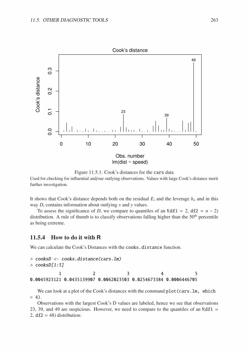
11.5. OTHER DIAGNOSTIC TOOLS 263
0 10 20 30 40 50
0.0
0.1
0.2
0.3
Obs. number
Cook’
s dis
tance
lm(dist ~ speed)
Cook’s distance
49
2339
Figure 11.5.1: Cook’s distances for the cars dataUsed for checking for influential and/our outlying observations. Values with large Cook’s distance merit
further investigation.
It shows that Cook’s distance depends both on the residual Ei and the leverage hii and in thisway Di contains information about outlying x and y values.
To assess the significance of D, we compare to quantiles of an f(df1 = 2, df2 = n # 2)distribution. A rule of thumb is to classify observations falling higher than the 50th percentileas being extreme.
11.5.4 How to do it with R
We can calculate the Cook’s Distances with the cooks.distance function.
> cooksD <- cooks.distance(cars.lm)
> cooksD[1:5]
1 2 3 4 5
0.0045923121 0.0435139907 0.0062023503 0.0254673384 0.0006446705
We can look at a plot of the Cook’s distances with the command plot(cars.lm, which= 4).
Observations with the largest Cook’s D values are labeled, hence we see that observations23, 39, and 49 are suspicious. However, we need to compare to the quantiles of an f(df1 =2, df2 = 48) distribution:
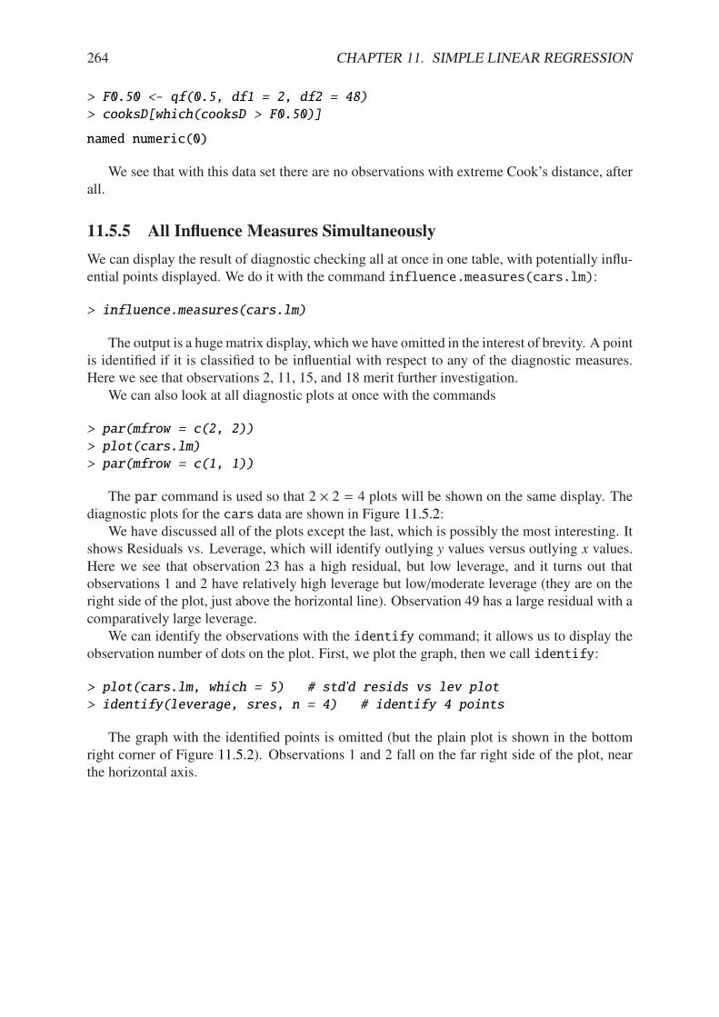
264 CHAPTER 11. SIMPLE LINEAR REGRESSION
> F0.50 <- qf(0.5, df1 = 2, df2 = 48)
> cooksD[which(cooksD > F0.50)]
named numeric(0)
We see that with this data set there are no observations with extreme Cook’s distance, afterall.
11.5.5 All Influence Measures Simultaneously
We can display the result of diagnostic checking all at once in one table, with potentially influ-ential points displayed. We do it with the command influence.measures(cars.lm):
> influence.measures(cars.lm)
The output is a hugematrix display, which we have omitted in the interest of brevity. A pointis identified if it is classified to be influential with respect to any of the diagnostic measures.Here we see that observations 2, 11, 15, and 18 merit further investigation.
We can also look at all diagnostic plots at once with the commands
> par(mfrow = c(2, 2))
> plot(cars.lm)
> par(mfrow = c(1, 1))
The par command is used so that 2 7 2 = 4 plots will be shown on the same display. Thediagnostic plots for the cars data are shown in Figure 11.5.2:
We have discussed all of the plots except the last, which is possibly the most interesting. Itshows Residuals vs. Leverage, which will identify outlying y values versus outlying x values.Here we see that observation 23 has a high residual, but low leverage, and it turns out thatobservations 1 and 2 have relatively high leverage but low/moderate leverage (they are on theright side of the plot, just above the horizontal line). Observation 49 has a large residual with acomparatively large leverage.
We can identify the observations with the identify command; it allows us to display theobservation number of dots on the plot. First, we plot the graph, then we call identify:
> plot(cars.lm, which = 5) # std'd resids vs lev plot> identify(leverage, sres, n = 4) # identify 4 points
The graph with the identified points is omitted (but the plain plot is shown in the bottomright corner of Figure 11.5.2). Observations 1 and 2 fall on the far right side of the plot, nearthe horizontal axis.
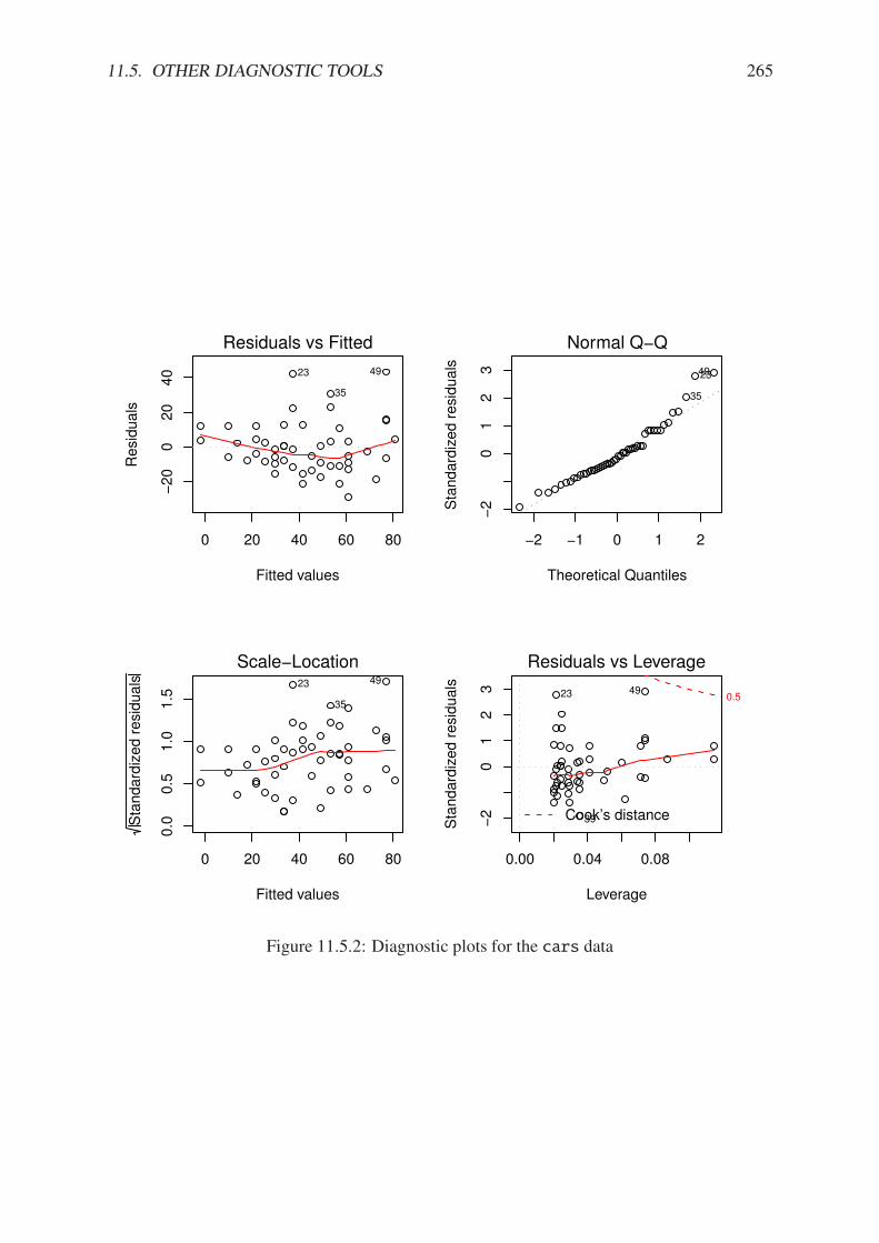
11.5. OTHER DIAGNOSTIC TOOLS 265
0 20 40 60 80
!20
020
40
Fitted values
Resi
duals
Residuals vs Fitted
4923
35
!2 !1 0 1 2
!2
01
23
Theoretical Quantiles
Sta
ndard
ized r
esi
duals
Normal Q!Q
4923
35
0 20 40 60 80
0.0
0.5
1.0
1.5
Fitted values
Sta
ndard
ized r
esi
duals
Scale!Location4923
35
0.00 0.04 0.08
!2
01
23
Leverage
Sta
ndard
ized r
esi
duals
Cook’s distance
0.5
Residuals vs Leverage
4923
39
Figure 11.5.2: Diagnostic plots for the cars data
266 CHAPTER 11. SIMPLE LINEAR REGRESSION
Chapter Exercises
Exercise 11.1. Prove the ANOVA equality, Equation 11.3.5. Hint: show that
n!
i=1
(Yi # Yi)(Yi # Y) = 0.
Exercise 11.2. Solve the following system of equations for *1 and *0 to find the MLEs forslope and intercept in the simple linear regression model.
n*0 + *1
n!
i=1
xi =
n!
i=1
yi
*0
n!
i=1
xi + *1
n!
i=1
x2i =
n!
i=1
xiyi
Exercise 11.3. Show that the formula given in Equation 11.2.17 is equivalent to
*1 =
#ni=1 xiyi #
=#ni=1 xi
> =#ni=1 yi
>Zn
#ni=1 x
2i #
=#ni=1 xi
>2Tn
.
Chapter 12
Multiple Linear Regression
We know a lot about simple linear regression models, and a next step is to study multiple re-gression models that have more than one independent (explanatory) variable. In the discussionthat follows we will assume that we have p explanatory variables, where p > 1.
The language is phrased in matrix terms – for two reasons. First, it is quicker to write and(arguably) more pleasant to read. Second, the matrix approach will be required for later studyof the subject; the reader might as well be introduced to it now.
Most of the results are stated without proof or with only a cursory justification. Thoseyearning for more should consult an advanced text in linear regression for details, such asApplied Linear Regression Models [67]or Linear Models: Least Squares and Alternatives [69].
What do I want them to know?
• the basic MLR model, and how it relates to the SLR
• how to estimate the parameters and use those estimates to make predictions
• basic strategies to determine whether or not the model is doing a good job
• a few thoughts about selected applications of the MLR, such as polynomial, interaction,and dummy variable models
• some of the uses of residuals to diagnose problems
• hints about what will be coming later
12.1 The Multiple Linear Regression Model
The first thing to do is get some better notation. We will write
Yn71 =
EFFFFFFFFFFFFFFFG
y1y2...
yn
HIIIIIIIIIIIIIIIJ, and Xn7(p+1) =
EFFFFFFFFFFFFFFFG
1 x11 x21 · · · xp11 x12 x22 · · · xp2......
.... . .
...
1 x1n x2n · · · xpn
HIIIIIIIIIIIIIIIJ. (12.1.1)
The vector Y is called the response vector and the matrix X is called the model matrix. As inChapter 11, the most general assumption that relates Y to X is
Y = µ(X) + !, (12.1.2)
267
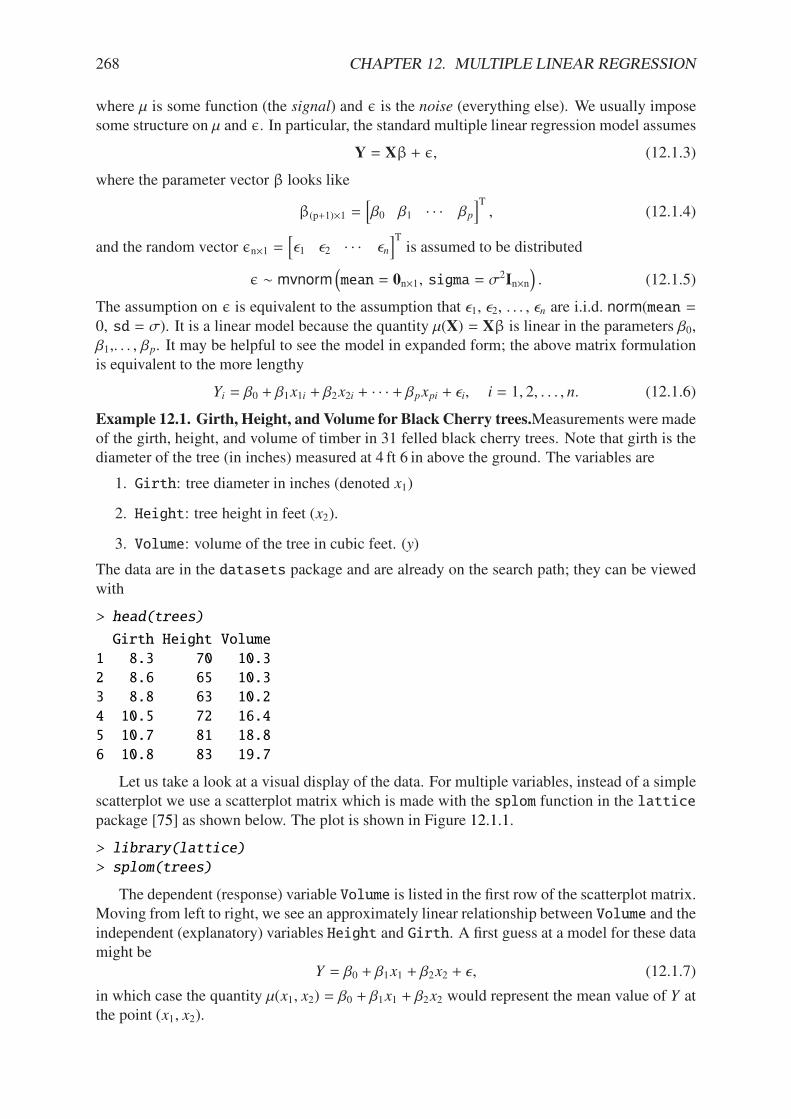
268 CHAPTER 12. MULTIPLE LINEAR REGRESSION
where µ is some function (the signal) and ! is the noise (everything else). We usually imposesome structure on µ and !. In particular, the standard multiple linear regression model assumes
Y = X" + !, (12.1.3)
where the parameter vector " looks like
"(p+1)71 =C*0 *1 · · · *p
DT, (12.1.4)
and the random vector !n71 =C$1 $2 · · · $n
DTis assumed to be distributed
! 4 mvnorm2mean = 0n71, sigma = "
2In7n3. (12.1.5)
The assumption on ! is equivalent to the assumption that $1, $2, . . . , $n are i.i.d. norm(mean =0, sd = "). It is a linear model because the quantity µ(X) = X" is linear in the parameters *0,*1,. . . , *p. It may be helpful to see the model in expanded form; the above matrix formulationis equivalent to the more lengthy
Yi = *0 + *1x1i + *2x2i + · · · + *pxpi + $i, i = 1, 2, . . . , n. (12.1.6)
Example 12.1. Girth, Height, and Volume for Black Cherry trees.Measurements were madeof the girth, height, and volume of timber in 31 felled black cherry trees. Note that girth is thediameter of the tree (in inches) measured at 4 ft 6 in above the ground. The variables are
1. Girth: tree diameter in inches (denoted x1)
2. Height: tree height in feet (x2).
3. Volume: volume of the tree in cubic feet. (y)
The data are in the datasets package and are already on the search path; they can be viewedwith
> head(trees)
Girth Height Volume
1 8.3 70 10.3
2 8.6 65 10.3
3 8.8 63 10.2
4 10.5 72 16.4
5 10.7 81 18.8
6 10.8 83 19.7
Let us take a look at a visual display of the data. For multiple variables, instead of a simplescatterplot we use a scatterplot matrix which is made with the splom function in the latticepackage [75] as shown below. The plot is shown in Figure 12.1.1.
> library(lattice)
> splom(trees)
The dependent (response) variable Volume is listed in the first row of the scatterplot matrix.Moving from left to right, we see an approximately linear relationship between Volume and theindependent (explanatory) variables Height and Girth. A first guess at a model for these datamight be
Y = *0 + *1x1 + *2x2 + $, (12.1.7)
in which case the quantity µ(x1, x2) = *0 + *1x1 + *2x2 would represent the mean value of Y atthe point (x1, x2).
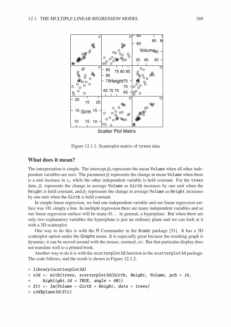
12.1. THE MULTIPLE LINEAR REGRESSION MODEL 269
Scatter Plot Matrix
Girth15
2015 20
10
15
10 15
Height75
80
85 75 80 85
65
70
75
65 70 75
Volume
60
80
60 80
20
40
20 40
Figure 12.1.1: Scatterplot matrix of trees data
What does it mean?
The interpretation is simple. The intercept *0 represents the mean Volume when all other inde-pendent variables are zero. The parameter *i represents the change in mean Volume when thereis a unit increase in xi, while the other independent variable is held constant. For the treesdata, *1 represents the change in average Volume as Girth increases by one unit when theHeight is held constant, and *2 represents the change in average Volume as Height increasesby one unit when the Girth is held constant.
In simple linear regression, we had one independent variable and our linear regression sur-face was 1D, simply a line. In multiple regression there are many independent variables and soour linear regression surface will be many-D. . . in general, a hyperplane. But when there areonly two explanatory variables the hyperplane is just an ordinary plane and we can look at itwith a 3D scatterplot.
One way to do this is with the R Commander in the Rcmdr package [31]. It has a 3Dscatterplot option under the Graphs menu. It is especially great because the resulting graph isdynamic; it can be moved around with the mouse, zoomed, etc. But that particular display doesnot translate well to a printed book.
Another way to do it is with the scatterplot3d function in the scatterplot3d package.The code follows, and the result is shown in Figure 12.1.2.
> library(scatterplot3d)
> s3d <- with(trees, scatterplot3d(Girth, Height, Volume, pch = 16,
+ highlight.3d = TRUE, angle = 60))
> fit <- lm(Volume ~ Girth + Height, data = trees)
> s3d$plane3d(fit)
270 CHAPTER 12. MULTIPLE LINEAR REGRESSION
8 10 12 14 16 18 20 2210
20
30
40
50
60
70
80
6065
7075
8085
90
Girth
Heig
ht
Volu
me
Figure 12.1.2: 3D scatterplot with regression plane for the trees data
Looking at the graph we see that the data points fall close to a plane in three dimensionalspace. (The plot looks remarkably good. In the author’s experience it is rare to see points fit sowell to the plane without some additional work.)
12.2 Estimation and Prediction
12.2.1 Parameter estimates
We will proceed exactly like we did in Section 11.2. We know
! 4 mvnorm2mean = 0n71, sigma = "
2In7n3, (12.2.1)
which means that Y = X" + ! has an mvnorm2mean = X", sigma = "2In7n
3distribution.
Therefore, the likelihood function is
L(",") =1
2&n/2"exp
.#
1
2"2(Y # X")T (Y # X")
/. (12.2.2)
Tomaximize the likelihood in", we need tominimize the quantity g(") = (Y # X")T (Y # X").We do this by di!erentiating g with respect to ". (It may be a good idea to brush up on thematerial in Appendices E.5 and E.6.) First we will rewrite g:
g(") = YTY # YTX" # "TXTY + "TXTX", (12.2.3)
which can be further simplified to g(") = YTY # 2"TXTY + "TXTX" since "TXTY is 1 7 1and thus equal to its transpose. Now we di!erentiate to get
-g
-"= 0 # 2XTY + 2XTX", (12.2.4)

12.2. ESTIMATION AND PREDICTION 271
since XTX is symmetric. Setting the derivative equal to the zero vector yields the so called“normal equations”
XTX" = XTY. (12.2.5)
In the case that XTX is invertible1, we may solve the equation for " to get the maximumlikelihood estimator of " which we denote by b:
b =2XTX
3#1XTY. (12.2.6)
Remark 12.2. The formula in Equation 12.2.6 is convenient for mathematical study but is incon-venient for numerical computation. Researchers have devised much more e"cient algorithmsfor the actual calculation of the parameter estimates, and we do not explore them here.
Remark 12.3. We have only found a critical value, and have not actually shown that the criticalvalue is a minimum. We omit the details and refer the interested reader to [69].
12.2.2 How to do it with R
We do all of the above just as we would in simple linear regression. The powerhouse is thelm function. Everything else is based on it. We separate explanatory variables in the modelformula by a plus sign.
> trees.lm <- lm(Volume ~ Girth + Height, data = trees)
> trees.lm
Call:
lm(formula = Volume ~ Girth + Height, data = trees)
Coefficients:
(Intercept) Girth Height
-57.9877 4.7082 0.3393
We see from the output that for the trees data our parameter estimates are b =C#58.0 4.7 0.3
D,
and consequently our estimate of the mean response is µ given by
µ(x1, x2) = b0 + b1x1 + b2x2, (12.2.7)
' # 58.0 + 4.7x1 + 0.3x2. (12.2.8)
We could see the entire model matrix X with the model.matrix function, but in the interest ofbrevity we only show the first few rows.
> head(model.matrix(trees.lm))
(Intercept) Girth Height
1 1 8.3 70
2 1 8.6 65
3 1 8.8 63
4 1 10.5 72
5 1 10.7 81
6 1 10.8 83
1We can find solutions of the normal equations even when XTX is not of full rank, but the topic falls outsidethe scope of this book. The interested reader can consult an advanced text such as Rao [69].
272 CHAPTER 12. MULTIPLE LINEAR REGRESSION
12.2.3 Point Estimates of the Regression Surface
The parameter estimates b make it easy to find the fitted values, Y. We write them individuallyas Yi, i = 1, 2, . . . , n, and recall that they are defined by
Yi = µ(x1i, x2i), (12.2.9)
= b0 + b1x1i + b2x2i, i = 1, 2, . . . , n. (12.2.10)
They are expressed more compactly by the matrix equation
Y = Xb. (12.2.11)
From Equation 12.2.6 we know that b =2XTX
3#1XTY, so we can rewrite
Y = XK2XTX
3#1XTY
L, (12.2.12)
= HY, (12.2.13)
whereH = X2XTX
3#1XT is appropriately named the hat matrix because it “puts the hat on Y”.
The hat matrix is very important in later courses. Some facts about H are
• H is a symmetric square matrix, of dimension n 7 n.
• The diagonal entries hii satisfy 0 " hii " 1 (compare to Equation 11.5.2).
• The trace is tr(H) = p.
• H is idempotent (also known as a projection matrix) which means that H2 = H. Thesame is true of I #H.
Now let us write a column vector x0 = (x10, x20)T to denote given values of the explanatory
variables Girth = x10 and Height = x20. These values may match those of the collected data,or they may be completely new values not observed in the original data set. We may use theparameter estimates to find Y(x0), which will give us
1. an estimate of µ(x0), the mean value of a future observation at x0, and
2. a prediction for Y(x0), the actual value of a future observation at x0.
We can represent Y(x0) by the matrix equation
Y(x0) = xT0b, (12.2.14)
which is just a fancy way to write
Y(x10, x20) = b0 + b1x10 + b2x20. (12.2.15)
Example 12.4. If we wanted to predict the average volume of black cherry trees that haveGirth = 15 in and are Height = 77 ft tall then we would use the estimate
µ(15, 77) = # 58 + 4.7(15) + 0.3(77),
'35.6 ft3.
We would use the same estimate Y = 35.6 to predict the measured Volume of another blackcherry tree – yet to be observed – that has Girth = 15 in and is Height = 77 ft tall.
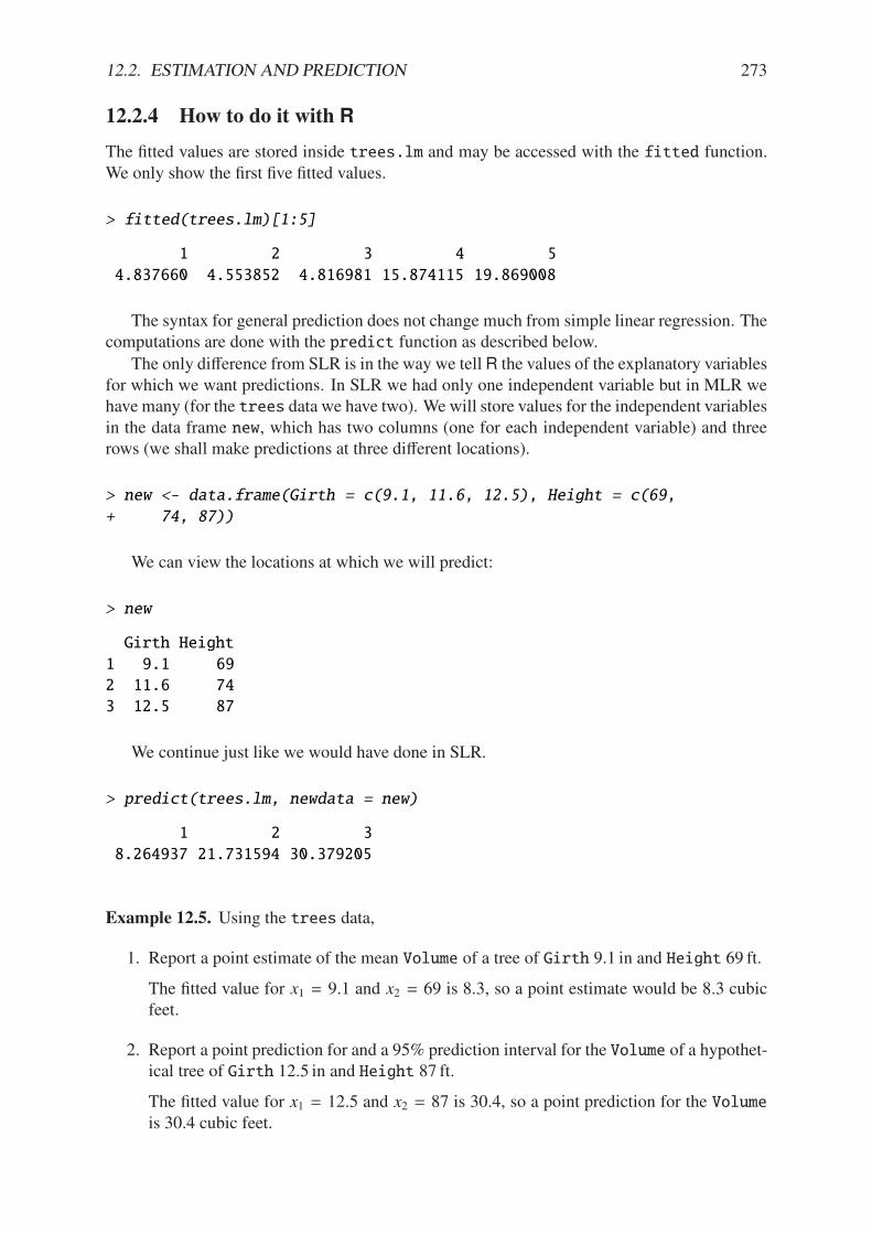
12.2. ESTIMATION AND PREDICTION 273
12.2.4 How to do it with R
The fitted values are stored inside trees.lm and may be accessed with the fitted function.We only show the first five fitted values.
> fitted(trees.lm)[1:5]
1 2 3 4 5
4.837660 4.553852 4.816981 15.874115 19.869008
The syntax for general prediction does not change much from simple linear regression. Thecomputations are done with the predict function as described below.
The only di!erence from SLR is in the way we tell R the values of the explanatory variablesfor which we want predictions. In SLR we had only one independent variable but in MLR wehave many (for the trees data we have two). We will store values for the independent variablesin the data frame new, which has two columns (one for each independent variable) and threerows (we shall make predictions at three di!erent locations).
> new <- data.frame(Girth = c(9.1, 11.6, 12.5), Height = c(69,
+ 74, 87))
We can view the locations at which we will predict:
> new
Girth Height
1 9.1 69
2 11.6 74
3 12.5 87
We continue just like we would have done in SLR.
> predict(trees.lm, newdata = new)
1 2 3
8.264937 21.731594 30.379205
Example 12.5. Using the trees data,
1. Report a point estimate of the mean Volume of a tree of Girth 9.1 in and Height 69 ft.
The fitted value for x1 = 9.1 and x2 = 69 is 8.3, so a point estimate would be 8.3 cubicfeet.
2. Report a point prediction for and a 95% prediction interval for the Volume of a hypothet-ical tree of Girth 12.5 in and Height 87 ft.
The fitted value for x1 = 12.5 and x2 = 87 is 30.4, so a point prediction for the Volumeis 30.4 cubic feet.
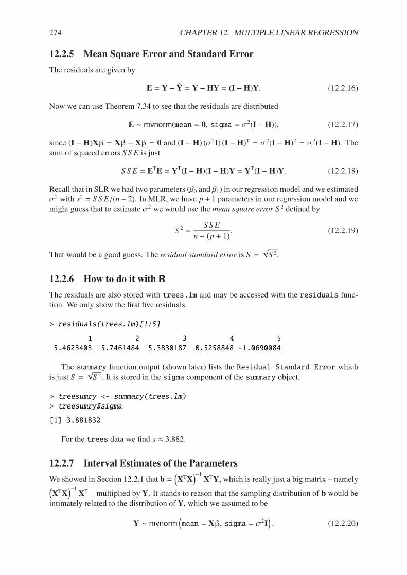
274 CHAPTER 12. MULTIPLE LINEAR REGRESSION
12.2.5 Mean Square Error and Standard Error
The residuals are given by
E = Y # Y = Y #HY = (I #H)Y. (12.2.16)
Now we can use Theorem 7.34 to see that the residuals are distributed
E 4 mvnorm(mean = 0, sigma = "2(I #H)), (12.2.17)
since (I # H)X" = X" # X" = 0 and (I # H) ("2I) (I # H)T = "2(I # H)2 = "2(I # H). Thesum of squared errors S S E is just
S S E = ETE = YT(I #H)(I #H)Y = YT(I #H)Y. (12.2.18)
Recall that in SLR we had two parameters (*0 and *1) in our regression model and we estimated"2 with s2 = S S E/(n # 2). In MLR, we have p + 1 parameters in our regression model and wemight guess that to estimate "2 we would use the mean square error S 2 defined by
S 2 =S S E
n # (p + 1). (12.2.19)
That would be a good guess. The residual standard error is S =$S 2.
12.2.6 How to do it with R
The residuals are also stored with trees.lm and may be accessed with the residuals func-tion. We only show the first five residuals.
> residuals(trees.lm)[1:5]
1 2 3 4 5
5.4623403 5.7461484 5.3830187 0.5258848 -1.0690084
The summary function output (shown later) lists the Residual Standard Error whichis just S =
$S 2. It is stored in the sigma component of the summary object.
> treesumry <- summary(trees.lm)
> treesumry$sigma
[1] 3.881832
For the trees data we find s ' 3.882.
12.2.7 Interval Estimates of the Parameters
We showed in Section 12.2.1 that b =2XTX
3#1XTY, which is really just a big matrix – namely
2XTX
3#1XT – multiplied by Y. It stands to reason that the sampling distribution of b would be
intimately related to the distribution of Y, which we assumed to be
Y 4 mvnorm2mean = X", sigma = "2I
3. (12.2.20)
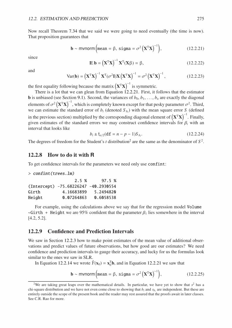
12.2. ESTIMATION AND PREDICTION 275
Now recall Theorem 7.34 that we said we were going to need eventually (the time is now).That proposition guarantees that
b 4 mvnorm?mean = ", sigma = "2
2XTX
3#1@, (12.2.21)
sinceIE b =
2XTX
3#1XT(X") = ", (12.2.22)
andVar(b) =
2XTX
3#1XT("2I)X
2XTX
3#1= "2
2XTX
3#1, (12.2.23)
the first equality following because the matrix2XTX
3#1is symmetric.
There is a lot that we can glean from Equation 12.2.21. First, it follows that the estimatorb is unbiased (see Section 9.1). Second, the variances of b0, b1, . . . , bn are exactly the diagonal
elements of "22XTX
3#1, which is completely known except for that pesky parameter "2. Third,
we can estimate the standard error of bi (denoted S bi) with the mean square error S (defined
in the previous section) multiplied by the corresponding diagonal element of2XTX
3#1. Finally,
given estimates of the standard errors we may construct confidence intervals for *i with aninterval that looks like
bi ± t(/2(df = n # p # 1)S bi . (12.2.24)
The degrees of freedom for the Student’s t distribution2 are the same as the denominator of S 2.
12.2.8 How to do it with R
To get confidence intervals for the parameters we need only use confint:
> confint(trees.lm)
2.5 % 97.5 %
(Intercept) -75.68226247 -40.2930554
Girth 4.16683899 5.2494820
Height 0.07264863 0.6058538
For example, using the calculations above we say that for the regression model Volume~Girth + Height we are 95% confident that the parameter *1 lies somewhere in the interval[4.2, 5.2].
12.2.9 Confidence and Prediction Intervals
We saw in Section 12.2.3 how to make point estimates of the mean value of additional obser-vations and predict values of future observations, but how good are our estimates? We needconfidence and prediction intervals to gauge their accuracy, and lucky for us the formulas looksimilar to the ones we saw in SLR.
In Equation 12.2.14 we wrote Y(x0) = xT0b, and in Equation 12.2.21 we saw that
b 4 mvnorm?mean = ", sigma = "2
2XTX
3#1@, (12.2.25)
2We are taking great leaps over the mathematical details. In particular, we have yet to show that s2 has achi-square distribution and we have not even come close to showing that bi and sbi are independent. But these areentirely outside the scope of the present book and the reader may rest assured that the proofs await in later classes.See C.R. Rao for more.
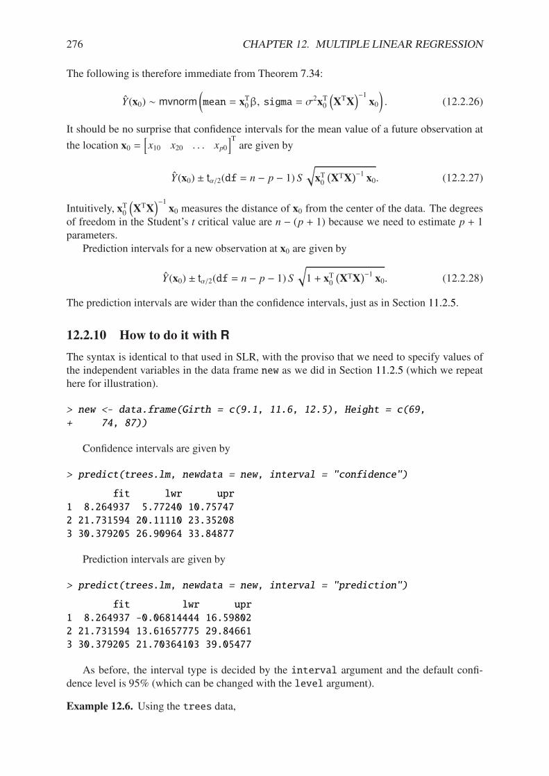
276 CHAPTER 12. MULTIPLE LINEAR REGRESSION
The following is therefore immediate from Theorem 7.34:
Y(x0) 4 mvnorm?mean = xT0", sigma = "
2xT02XTX
3#1x0
@. (12.2.26)
It should be no surprise that confidence intervals for the mean value of a future observation at
the location x0 =Cx10 x20 . . . xp0
DTare given by
Y(x0) ± t(/2(df = n # p # 1) S
MxT0
=XTX
>#1 x0. (12.2.27)
Intuitively, xT02XTX
3#1x0 measures the distance of x0 from the center of the data. The degrees
of freedom in the Student’s t critical value are n # (p + 1) because we need to estimate p + 1parameters.
Prediction intervals for a new observation at x0 are given by
Y(x0) ± t(/2(df = n # p # 1) S
M1 + xT0
=XTX
>#1 x0. (12.2.28)
The prediction intervals are wider than the confidence intervals, just as in Section 11.2.5.
12.2.10 How to do it with R
The syntax is identical to that used in SLR, with the proviso that we need to specify values ofthe independent variables in the data frame new as we did in Section 11.2.5 (which we repeathere for illustration).
> new <- data.frame(Girth = c(9.1, 11.6, 12.5), Height = c(69,
+ 74, 87))
Confidence intervals are given by
> predict(trees.lm, newdata = new, interval = "confidence")
fit lwr upr
1 8.264937 5.77240 10.75747
2 21.731594 20.11110 23.35208
3 30.379205 26.90964 33.84877
Prediction intervals are given by
> predict(trees.lm, newdata = new, interval = "prediction")
fit lwr upr
1 8.264937 -0.06814444 16.59802
2 21.731594 13.61657775 29.84661
3 30.379205 21.70364103 39.05477
As before, the interval type is decided by the interval argument and the default confi-dence level is 95% (which can be changed with the level argument).
Example 12.6. Using the trees data,
12.3. MODEL UTILITY AND INFERENCE 277
1. Report a 95% confidence interval for the mean Volume of a tree of Girth 9.1 in andHeight 69 ft.
The 95% CI is given by [5.8, 10.8], so with 95% confidence the mean Volume lies some-where between 5.8 cubic feet and 10.8 cubic feet.
2. Report a 95% prediction interval for the Volume of a hypothetical tree of Girth 12.5 inand Height 87 ft.
The 95% prediction interval is given by [26.9, 33.8], so with 95% confidence we mayassert that the hypothetical Volume of a tree of Girth 12.5 in and Height 87 ft would liesomewhere between 26.9 cubic feet and 33.8 feet.
12.3 Model Utility and Inference
12.3.1 Multiple Coe"cient of Determination
We saw in Section 12.2.5 that the error sum of squares S S E can be conveniently written inMLR as
S S E = YT(I #H)Y. (12.3.1)
It turns out that there are equally convenient formulas for the total sum of squares S S TO andthe regression sum of squares S SR. They are :
S S TO =YT
0I #
1
nJ
1Y (12.3.2)
and
S SR =YT
0H #
1
nJ
1Y. (12.3.3)
(The matrix J is defined in Appendix E.5.) Immediately from Equations 12.3.1, 12.3.2, and12.3.3 we get the Anova Equality
S S TO = S S E + S SR. (12.3.4)
(See Exercise 12.1.) We define the multiple coe!cient of determination by the formula
R2 = 1 #S S E
S S TO. (12.3.5)
We interpret R2 as the proportion of total variation that is explained by the multiple regres-sion model. In MLR we must be careful, however, because the value of R2 can be artificiallyinflated by the addition of explanatory variables to the model, regardless of whether or not theadded variables are useful with respect to prediction of the response variable. In fact, it can beproved that the addition of a single explanatory variable to a regression model will increase thevalue of R2, no matter how worthless the explanatory variable is. We could model the heightof the ocean tides, then add a variable for the length of cheetah tongues on the Serengeti plain,and our R2 would inevitably increase.
278 CHAPTER 12. MULTIPLE LINEAR REGRESSION
This is a problem, because as the philosopher, Occam, once said: “causes should not bemultiplied beyond necessity”. We address the problem by penalizing R2 when parameters are
added to the model. The result is an adjusted R2 which we denote by R2.
R2=
?R2 #
p
n # 1
@ 0n # 1
n # p # 1
1. (12.3.6)
It is good practice for the statistician to weigh bothR2 and R2during assessment of model utility.
In many cases their values will be very close to each other. If their values di!er substantially,or if one changes dramatically when an explanatory variable is added, then (s)he should take acloser look at the explanatory variables in the model.
12.3.2 How to do it with R
For the trees data, we can get R2 and R2from the summary output or access the values directly
by name as shown (recall that we stored the summary object in treesumry).
> treesumry$r.squared
[1] 0.94795
> treesumry$adj.r.squared
[1] 0.9442322
High values of R2 and R2such as these indicate that the model fits very well, which agrees
with what we saw in Figure 12.1.2.
12.3.3 Overall F-Test
Another way to assess the model’s utility is to to test the hypothesis
H0 : *1 = *2 = · · · = *p = 0 versus H1 : at least one *i ! 0.
The idea is that if all *i’s were zero, then the explanatory variables X1, . . . , Xp would be worth-less predictors for the response variable Y . We can test the above hypothesis with the overall Fstatistic, which in MLR is defined by
F =S SR/p
S S E/(n # p # 1). (12.3.7)
When the regression assumptions hold and under H0, it can be shown that F 4 f(df1 =p, df2 = n # p # 1). We reject H0 when F is large, that is, when the explained variationis large relative to the unexplained variation.
12.3.4 How to do it with R
The overall F statistic and its associated p-value is listed at the bottom of the summary output,or we can access it directly by name; it is stored in the fstatistic component of the summaryobject.
> treesumry$fstatistic
value numdf dendf
254.9723 2.0000 28.0000
For the trees data, we see that F = 254.972337410669 with a p-value < 2.2e-16. Con-sequently we reject H0, that is, the data provide strong evidence that not all *i’s are zero.
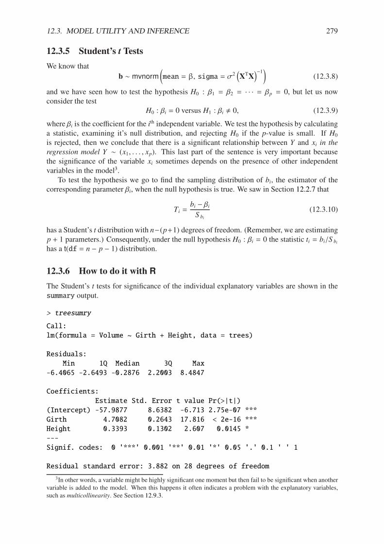
12.3. MODEL UTILITY AND INFERENCE 279
12.3.5 Student’s t Tests
We know that
b 4 mvnorm?mean = ", sigma = "2
2XTX
3#1@(12.3.8)
and we have seen how to test the hypothesis H0 : *1 = *2 = · · · = *p = 0, but let us nowconsider the test
H0 : *i = 0 versus H1 : *i ! 0, (12.3.9)
where *i is the coe"cient for the ith independent variable. We test the hypothesis by calculating
a statistic, examining it’s null distribution, and rejecting H0 if the p-value is small. If H0
is rejected, then we conclude that there is a significant relationship between Y and xi in the
regression model Y 4 (x1, . . . , xp). This last part of the sentence is very important becausethe significance of the variable xi sometimes depends on the presence of other independentvariables in the model3.
To test the hypothesis we go to find the sampling distribution of bi, the estimator of thecorresponding parameter *i, when the null hypothesis is true. We saw in Section 12.2.7 that
Ti =bi # *iS bi
(12.3.10)
has a Student’s t distribution with n#(p+1) degrees of freedom. (Remember, we are estimatingp + 1 parameters.) Consequently, under the null hypothesis H0 : *i = 0 the statistic ti = bi/S bi
has a t(df = n # p # 1) distribution.
12.3.6 How to do it with R
The Student’s t tests for significance of the individual explanatory variables are shown in thesummary output.
> treesumry
Call:
lm(formula = Volume ~ Girth + Height, data = trees)
Residuals:
Min 1Q Median 3Q Max
-6.4065 -2.6493 -0.2876 2.2003 8.4847
Coefficients:
Estimate Std. Error t value Pr(>|t|)
(Intercept) -57.9877 8.6382 -6.713 2.75e-07 ***
Girth 4.7082 0.2643 17.816 < 2e-16 ***
Height 0.3393 0.1302 2.607 0.0145 *
---
Signif. codes: 0 '***' 0.001 '**' 0.01 '*' 0.05 '.' 0.1 ' ' 1
Residual standard error: 3.882 on 28 degrees of freedom
3In other words, a variable might be highly significant one moment but then fail to be significant when anothervariable is added to the model. When this happens it often indicates a problem with the explanatory variables,such as multicollinearity. See Section 12.9.3.
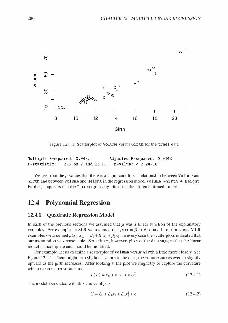
280 CHAPTER 12. MULTIPLE LINEAR REGRESSION
8 10 12 14 16 18 20
10
30
50
70
Girth
Volu
me
Figure 12.4.1: Scatterplot of Volume versus Girth for the trees data
Multiple R-squared: 0.948, Adjusted R-squared: 0.9442
F-statistic: 255 on 2 and 28 DF, p-value: < 2.2e-16
We see from the p-values that there is a significant linear relationship between Volume andGirth and between Volume and Height in the regression model Volume ~Girth + Height.Further, it appears that the Intercept is significant in the aforementioned model.
12.4 Polynomial Regression
12.4.1 Quadratic Regression Model
In each of the previous sections we assumed that µ was a linear function of the explanatoryvariables. For example, in SLR we assumed that µ(x) = *0 + *1x, and in our previous MLRexamples we assumed µ(x1, x2) = *0 + *1x1 + *2x2. In every case the scatterplots indicated thatour assumption was reasonable. Sometimes, however, plots of the data suggest that the linearmodel is incomplete and should be modified.
For example, let us examine a scatterplot of Volume versus Girth a little more closely. SeeFigure 12.4.1. There might be a slight curvature to the data; the volume curves ever so slightlyupward as the girth increases. After looking at the plot we might try to capture the curvaturewith a mean response such as
µ(x1) = *0 + *1x1 + *2x21. (12.4.1)
The model associated with this choice of µ is
Y = *0 + *1x1 + *2x21 + $. (12.4.2)
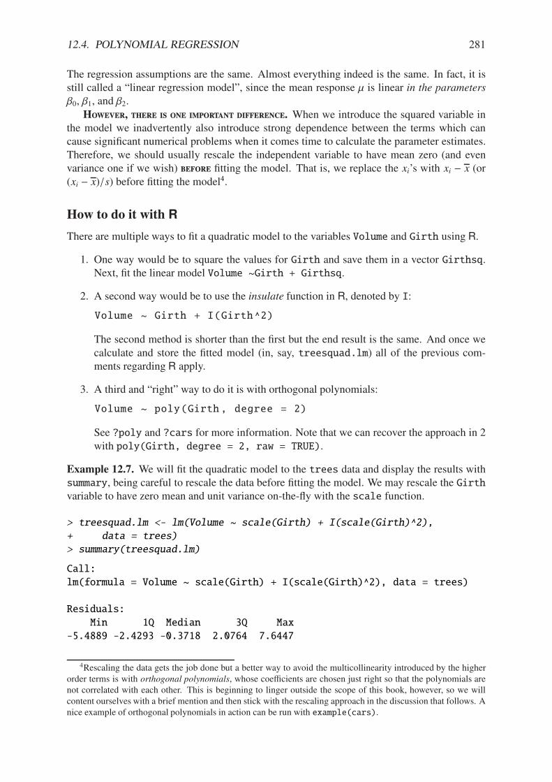
12.4. POLYNOMIAL REGRESSION 281
The regression assumptions are the same. Almost everything indeed is the same. In fact, it isstill called a “linear regression model”, since the mean response µ is linear in the parameters
*0, *1, and *2.However, there is one important difference. When we introduce the squared variable in
the model we inadvertently also introduce strong dependence between the terms which cancause significant numerical problems when it comes time to calculate the parameter estimates.Therefore, we should usually rescale the independent variable to have mean zero (and evenvariance one if we wish) before fitting the model. That is, we replace the xi’s with xi # x (or(xi # x)/s) before fitting the model4.
How to do it with R
There are multiple ways to fit a quadratic model to the variables Volume and Girth using R.
1. One way would be to square the values for Girth and save them in a vector Girthsq.Next, fit the linear model Volume ~Girth + Girthsq.
2. A second way would be to use the insulate function in R, denoted by I:
Volume ~ Girth + I(Girth^2)
The second method is shorter than the first but the end result is the same. And once wecalculate and store the fitted model (in, say, treesquad.lm) all of the previous com-ments regarding R apply.
3. A third and “right” way to do it is with orthogonal polynomials:
Volume ~ poly(Girth , degree = 2)
See ?poly and ?cars for more information. Note that we can recover the approach in 2with poly(Girth, degree = 2, raw = TRUE).
Example 12.7. We will fit the quadratic model to the trees data and display the results withsummary, being careful to rescale the data before fitting the model. We may rescale the Girthvariable to have zero mean and unit variance on-the-fly with the scale function.
> treesquad.lm <- lm(Volume ~ scale(Girth) + I(scale(Girth)^2),
+ data = trees)
> summary(treesquad.lm)
Call:
lm(formula = Volume ~ scale(Girth) + I(scale(Girth)^2), data = trees)
Residuals:
Min 1Q Median 3Q Max
-5.4889 -2.4293 -0.3718 2.0764 7.6447
4Rescaling the data gets the job done but a better way to avoid the multicollinearity introduced by the higherorder terms is with orthogonal polynomials, whose coe"cients are chosen just right so that the polynomials arenot correlated with each other. This is beginning to linger outside the scope of this book, however, so we willcontent ourselves with a brief mention and then stick with the rescaling approach in the discussion that follows. Anice example of orthogonal polynomials in action can be run with example(cars).
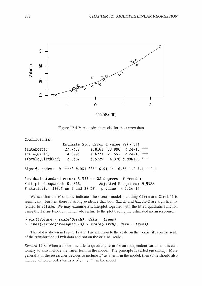
282 CHAPTER 12. MULTIPLE LINEAR REGRESSION
!1 0 1 2
10
30
50
70
scale(Girth)
Volu
me
Figure 12.4.2: A quadratic model for the trees data
Coefficients:
Estimate Std. Error t value Pr(>|t|)
(Intercept) 27.7452 0.8161 33.996 < 2e-16 ***
scale(Girth) 14.5995 0.6773 21.557 < 2e-16 ***
I(scale(Girth)^2) 2.5067 0.5729 4.376 0.000152 ***
---
Signif. codes: 0 '***' 0.001 '**' 0.01 '*' 0.05 '.' 0.1 ' ' 1
Residual standard error: 3.335 on 28 degrees of freedom
Multiple R-squared: 0.9616, Adjusted R-squared: 0.9588
F-statistic: 350.5 on 2 and 28 DF, p-value: < 2.2e-16
We see that the F statistic indicates the overall model including Girth and Girth^2 issignificant. Further, there is strong evidence that both Girth and Girth^2 are significantlyrelated to Volume. We may examine a scatterplot together with the fitted quadratic functionusing the lines function, which adds a line to the plot tracing the estimated mean response.
> plot(Volume ~ scale(Girth), data = trees)
> lines(fitted(treesquad.lm) ~ scale(Girth), data = trees)
The plot is shown in Figure 12.4.2. Pay attention to the scale on the x-axis: it is on the scaleof the transformed Girth data and not on the original scale.
Remark 12.8. When a model includes a quadratic term for an independent variable, it is cus-tomary to also include the linear term in the model. The principle is called parsimony. Moregenerally, if the researcher decides to include xm as a term in the model, then (s)he should alsoinclude all lower order terms x, x2, . . . ,xm#1 in the model.
12.5. INTERACTION 283
We do estimation/prediction the same way that we did in Section 12.2.3, except we do notneed a Height column in the dataframe new since the variable is not included in the quadraticmodel.
> new <- data.frame(Girth = c(9.1, 11.6, 12.5))
> predict(treesquad.lm, newdata = new, interval = "prediction")
fit lwr upr
1 11.56982 4.347426 18.79221
2 20.30615 13.299050 27.31325
3 25.92290 18.972934 32.87286
The predictions and intervals are slightly di!erent from what they were previously. Noticethat it was not necessary to rescale the Girth prediction data before input to the predictfunction; the model did the rescaling for us automatically.
Remark 12.9. We have mentioned on several occasions that it is important to rescale the ex-planatory variables for polynomial regression. Watch what happens if we ignore this advice:
> summary(lm(Volume ~ Girth + I(Girth^2), data = trees))
Call:
lm(formula = Volume ~ Girth + I(Girth^2), data = trees)
Residuals:
Min 1Q Median 3Q Max
-5.4889 -2.4293 -0.3718 2.0764 7.6447
Coefficients:
Estimate Std. Error t value Pr(>|t|)
(Intercept) 10.78627 11.22282 0.961 0.344728
Girth -2.09214 1.64734 -1.270 0.214534
I(Girth^2) 0.25454 0.05817 4.376 0.000152 ***
---
Signif. codes: 0 '***' 0.001 '**' 0.01 '*' 0.05 '.' 0.1 ' ' 1
Residual standard error: 3.335 on 28 degrees of freedom
Multiple R-squared: 0.9616, Adjusted R-squared: 0.9588
F-statistic: 350.5 on 2 and 28 DF, p-value: < 2.2e-16
Now nothing is significant in the model except Girth^2. We could delete the Interceptand Girth from the model, but the model would no longer be parsimonious. A novice may seethe output and be confused about how to proceed, while the seasoned statistician recognizesimmediately that Girth and Girth^2 are highly correlated (see Section 12.9.3). The onlyremedy to this ailment is to rescale Girth, which we should have done in the first place.
In Example 12.14 of Section 12.7 we investigate this issue further.
12.5 Interaction
In our model for tree volume there have been two independent variables: Girth and Height.We may suspect that the independent variables are related, that is, values of one variable may
284 CHAPTER 12. MULTIPLE LINEAR REGRESSION
tend to influence values of the other. It may be desirable to include an additional term in ourmodel to try and capture the dependence between the variables. Interaction terms are formedby multiplying one (or more) explanatory variable(s) by another.
Example 12.10. Perhaps the Girth and Height of the tree interact to influence the its Volume;we would like to investigate whether the model (Girth = x1 and Height = x2)
Y = *0 + *1x1 + *2x2 + $ (12.5.1)
would be significantly improved by the model
Y = *0 + *1x1 + *2x2 + *1:2x1x2 + $, (12.5.2)
where the subscript 1 : 2 denotes that *1:2 is a coe"cient of an interaction term between x1 andx2.
What does it mean? Consider the mean response µ(x1, x2) as a function of x2:
µ(x2) = (*0 + *1x1) + *2x2. (12.5.3)
This is a linear function of x2 with slope *2. As x1 changes, the y-intercept of the mean responsein x2 changes, but the slope remains the same. Therefore, the mean response in x2 is representedby a collection of parallel lines all with common slope *2.
Now think about what happens when the interaction term *1:2x1x2 is included. The meanresponse in x2 now looks like
µ(x2) = (*0 + *1x1) + (*2 + *1:2x1)x2. (12.5.4)
In this case we see that not only the y-intercept changes when x1 varies, but the slope alsochanges in x1. Thus, the interaction term allows the slope of the mean response in x2 to increaseand decrease as x1 varies.
How to do it with R
There are several ways to introduce an interaction term into the model.
1. Make a new variable prod <-Girth *Height, then include prod in the model formulaVolume ~Girth + Height + prod. This method is perhaps the most transparent, butit also reserves memory space unnecessarily.
2. Once can construct an interaction term directly in R with a colon “:”. For this example,the model formula would look like Volume ~Girth + Height + Girth:Height.
For the trees data, we fit the model with the interaction using method two and see if it issignificant:
> treesint.lm <- lm(Volume ~ Girth + Height + Girth:Height,
+ data = trees)
> summary(treesint.lm)
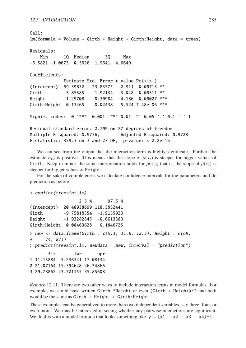
12.5. INTERACTION 285
Call:
lm(formula = Volume ~ Girth + Height + Girth:Height, data = trees)
Residuals:
Min 1Q Median 3Q Max
-6.5821 -1.0673 0.3026 1.5641 4.6649
Coefficients:
Estimate Std. Error t value Pr(>|t|)
(Intercept) 69.39632 23.83575 2.911 0.00713 **
Girth -5.85585 1.92134 -3.048 0.00511 **
Height -1.29708 0.30984 -4.186 0.00027 ***
Girth:Height 0.13465 0.02438 5.524 7.48e-06 ***
---
Signif. codes: 0 '***' 0.001 '**' 0.01 '*' 0.05 '.' 0.1 ' ' 1
Residual standard error: 2.709 on 27 degrees of freedom
Multiple R-squared: 0.9756, Adjusted R-squared: 0.9728
F-statistic: 359.3 on 3 and 27 DF, p-value: < 2.2e-16
We can see from the output that the interaction term is highly significant. Further, theestimate b1:2 is positive. This means that the slope of µ(x2) is steeper for bigger values ofGirth. Keep in mind: the same interpretation holds for µ(x1); that is, the slope of µ(x1) issteeper for bigger values of Height.
For the sake of completeness we calculate confidence intervals for the parameters and doprediction as before.
> confint(treesint.lm)
2.5 % 97.5 %
(Intercept) 20.48938699 118.3032441
Girth -9.79810354 -1.9135923
Height -1.93282845 -0.6613383
Girth:Height 0.08463628 0.1846725
> new <- data.frame(Girth = c(9.1, 11.6, 12.5), Height = c(69,
+ 74, 87))
> predict(treesint.lm, newdata = new, interval = "prediction")
fit lwr upr
1 11.15884 5.236341 17.08134
2 21.07164 15.394628 26.74866
3 29.78862 23.721155 35.85608
Remark 12.11. There are two other ways to include interaction terms in model formulas. Forexample, we could have written Girth *Height or even (Girth + Height)^2 and bothwould be the same as Girth + Height + Girth:Height.
These examples can be generalized to more than two independent variables, say three, four, oreven more. We may be interested in seeing whether any pairwise interactions are significant.We do this with a model formula that looks something like y ~ (x1 + x2 + x3 + x4)^2.
286 CHAPTER 12. MULTIPLE LINEAR REGRESSION
12.6 Qualitative Explanatory Variables
We have so far been concerned with numerical independent variables taking values in a subsetof real numbers. In this section, we extend our treatment to include the case in which one ofthe explanatory variables is qualitative, that is, a factor. Qualitative variables take values in aset of levels, which may or may not be ordered. See Section 3.1.2.
Note. The trees data do not have any qualitative explanatory variables, so we will constructone for illustrative purposes5. We will leave the Girth variable alone, but we will replace thevariable Height by a new variable Tall which indicates whether or not the cherry tree is tallerthan a certain threshold (which for the sake of argument will be the sample median height of76 ft). That is, Tall will be defined by
Tall =
9::;::<yes, if Height > 76,
no, if Height " 76.(12.6.1)
We can construct Tall very quickly in R with the cut function:
> trees$Tall <- cut(trees$Height, breaks = c(-Inf, 76, Inf),
+ labels = c("no", "yes"))
> trees$Tall[1:5]
[1] no no no no yes
Levels: no yes
Note that Tall is automatically generated to be a factor with the labels in the correct order.See ?cut for more.
Once we have Tall, we include it in the regression model just like we would any othervariable. It is handled internally in a special way. Define a “dummy variable” Tallyes thattakes values
Tallyes =
9::;::<1, if Tall = yes,
0, otherwise.(12.6.2)
That is, Tallyes is an indicator variable which indicates when a respective tree is tall. Themodel may now be written as
Volume = *0 + *1Girth + *2Tallyes + $. (12.6.3)
Let us take a look at what this definition does to the mean response. Trees with Tall = yeswill have the mean response
µ(Girth) = (*0 + *2) + *1Girth, (12.6.4)
while trees with Tall = no will have the mean response
µ(Girth) = *0 + *1Girth. (12.6.5)
In essence, we are fitting two regression lines: one for tall trees, and one for short trees. Theregression lines have the same slope but they have di!erent y intercepts (which are exactly |*2|far apart).
5This procedure of replacing a continuous variable by a discrete/qualitative one is called binning, and is almostnever the right thing to do. We are in a bind at this point, however, because we have invested this chapter in thetrees data and I do not want to switch mid-discussion. I am currently searching for a data set with pre-existingqualitative variables that also conveys the same points present in the trees data, and when I find it I will updatethis chapter accordingly.

12.6. QUALITATIVE EXPLANATORY VARIABLES 287
How to do it with R
The important thing is to double check that the qualitative variable in question is stored as afactor. The way to check is with the class command. For example,
> class(trees$Tall)
[1] "factor"
If the qualitative variable is not yet stored as a factor then we may convert it to one with thefactor command. See Section 3.1.2. Other than this we perform MLR as we normally would.
> treesdummy.lm <- lm(Volume ~ Girth + Tall, data = trees)
> summary(treesdummy.lm)
Call:
lm(formula = Volume ~ Girth + Tall, data = trees)
Residuals:
Min 1Q Median 3Q Max
-5.7788 -3.1710 0.4888 2.6737 10.0619
Coefficients:
Estimate Std. Error t value Pr(>|t|)
(Intercept) -34.1652 3.2438 -10.53 3.02e-11 ***
Girth 4.6988 0.2652 17.72 < 2e-16 ***
Tallyes 4.3072 1.6380 2.63 0.0137 *
---
Signif. codes: 0 '***' 0.001 '**' 0.01 '*' 0.05 '.' 0.1 ' ' 1
Residual standard error: 3.875 on 28 degrees of freedom
Multiple R-squared: 0.9481, Adjusted R-squared: 0.9444
F-statistic: 255.9 on 2 and 28 DF, p-value: < 2.2e-16
From the output we see that all parameter estimates are statistically significant and weconclude that the mean response di!ers for trees with Tall = yes and trees with Tall = no.
Remark 12.12. Wewere somewhat disingenuouswhenwe defined the dummy variable Tallyesbecause, in truth, R defines Tallyes automatically without input from the user6. Indeed, theauthor fit the model beforehand and wrote the discussion afterward with the knowledge of whatR would do so that the output the reader saw would match what (s)he had previously read. Theway that R handles factors internally is part of a much larger topic concerning contrasts, whichfalls outside the scope of this book. The interested reader should see Neter et al [67] or Fox[28] for more.
Remark 12.13. In general, if an explanatory variable foo is qualitative with n levels bar1,bar2, . . . , barn then R will by default automatically define n # 1 indicator variables in thefollowing way:
foobar2 =
9::;::<1, if foo = ”bar2”,
0, otherwise., . . . , foobarn =
9::;::<1, if foo = ”barn”,
0, otherwise.
6That is, R by default handles contrasts according to its internal settings which may be customized by the userfor fine control. Given that we will not investigate contrasts further in this book it does not serve the discussion todelve into those settings, either. The interested reader should check ?contrasts for details.
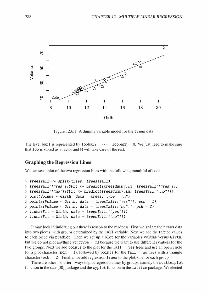
288 CHAPTER 12. MULTIPLE LINEAR REGRESSION
8 10 12 14 16 18 20
10
30
50
70
Girth
Volu
me
Figure 12.6.1: A dummy variable model for the trees data
The level bar1 is represented by foobar2 = · · · = foobarn = 0. We just need to make surethat foo is stored as a factor and R will take care of the rest.
Graphing the Regression Lines
We can see a plot of the two regression lines with the following mouthful of code.
> treesTall <- split(trees, trees$Tall)
> treesTall[["yes"]]$Fit <- predict(treesdummy.lm, treesTall[["yes"]])
> treesTall[["no"]]$Fit <- predict(treesdummy.lm, treesTall[["no"]])
> plot(Volume ~ Girth, data = trees, type = "n")
> points(Volume ~ Girth, data = treesTall[["yes"]], pch = 1)
> points(Volume ~ Girth, data = treesTall[["no"]], pch = 2)
> lines(Fit ~ Girth, data = treesTall[["yes"]])
> lines(Fit ~ Girth, data = treesTall[["no"]])
It may look intimidating but there is reason to the madness. First we split the trees datainto two pieces, with groups determined by the Tall variable. Next we add the Fitted valuesto each piece via predict. Then we set up a plot for the variables Volume versus Girth,but we do not plot anything yet (type = n) because we want to use di!erent symbols for thetwo groups. Next we add points to the plot for the Tall = yes trees and use an open circlefor a plot character (pch = 1), followed by points for the Tall = no trees with a trianglecharacter (pch = 2). Finally, we add regression lines to the plot, one for each group.
There are other – shorter – ways to plot regression lines by groups, namely the scatterplotfunction in the car [30] package and the xyplot function in the lattice package. We elected

12.7. PARTIAL F STATISTIC 289
to introduce the reader to the above approach since many advanced plots in R are done in asimilar, consecutive fashion.
12.7 Partial F Statistic
We saw in Section 12.3.3 how to test H0 : *0 = *1 = · · · = *p = 0 with the overall F statisticand we saw in Section 12.3.5 how to test H0 : *i = 0 that a particular coe"cient *i is zero.Sometimes, however, we would like to test whether a certain part of the model is significant.Consider the regression model
Y = *0 + *1x1 + · · · + * jx j + * j+1x j+1 + · · · + *pxp + $, (12.7.1)
where j / 1 and p / 2. Now we wish to test the hypothesis
H0 : * j+1 = * j+2 = · · · = *p = 0 (12.7.2)
versus the alternative
H1 : at least one of * j+1, * j+2, , . . . , *p ! 0. (12.7.3)
The interpretation of H0 is that none of the variables x j+1, . . . ,xp is significantly related to Y
and the interpretation of H1 is that at least one of x j+1, . . . ,xp is significantly related to Y . Inessence, for this hypothesis test there are two competing models under consideration:
the full model: y = *0 + *1x1 + · · · + *pxp + $, (12.7.4)
the reduced model: y = *0 + *1x1 + · · · + * jx j + $, (12.7.5)
Of course, the full model will always explain the data better than the reduced model, but doesthe full model explain the data significantly better than the reduced model? This question isexactly what the partial F statistic is designed to answer.
We first calculate S S E f , the unexplained variation in the full model, and S S Er, the unex-plained variation in the reduced model. We base our test on the di!erence S S Er#S S E f whichmeasures the reduction in unexplained variation attributable to the variables x j+1, . . . ,xp. In thefull model there are p+1 parameters and in the reduced model there are j+1 parameters, whichgives a di!erence of p # j parameters (hence degrees of freedom). The partial F statistic is
F =(S S Er # S S E f )/(p # j)
S S E f/(n # p # 1). (12.7.6)
It can be shown when the regression assumptions hold under H0 that the partial F statistic hasan f(df1 = p# j, df2 = n# p#1) distribution. We calculate the p-value of the observed partialF statistic and reject H0 if the p-value is small.
How to do it with R
The key ingredient above is that the two competing models are nested in the sense that thereduced model is entirely contained within the complete model. The way to test whether theimprovement is significant is to compute lm objects both for the complete model and the re-duced model then compare the answers with the anova function.
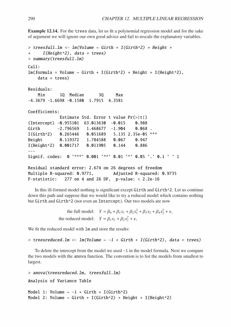
290 CHAPTER 12. MULTIPLE LINEAR REGRESSION
Example 12.14. For the trees data, let us fit a polynomial regression model and for the sakeof argument we will ignore our own good advice and fail to rescale the explanatory variables.
> treesfull.lm <- lm(Volume ~ Girth + I(Girth^2) + Height +
+ I(Height^2), data = trees)
> summary(treesfull.lm)
Call:
lm(formula = Volume ~ Girth + I(Girth^2) + Height + I(Height^2),
data = trees)
Residuals:
Min 1Q Median 3Q Max
-4.3679 -1.6698 -0.1580 1.7915 4.3581
Coefficients:
Estimate Std. Error t value Pr(>|t|)
(Intercept) -0.955101 63.013630 -0.015 0.988
Girth -2.796569 1.468677 -1.904 0.068 .
I(Girth^2) 0.265446 0.051689 5.135 2.35e-05 ***
Height 0.119372 1.784588 0.067 0.947
I(Height^2) 0.001717 0.011905 0.144 0.886
---
Signif. codes: 0 '***' 0.001 '**' 0.01 '*' 0.05 '.' 0.1 ' ' 1
Residual standard error: 2.674 on 26 degrees of freedom
Multiple R-squared: 0.9771, Adjusted R-squared: 0.9735
F-statistic: 277 on 4 and 26 DF, p-value: < 2.2e-16
In this ill-formed model nothing is significant except Girth and Girth^2. Let us continuedown this path and suppose that we would like to try a reduced model which contains nothingbut Girth and Girth^2 (not even an Intercept). Our two models are now
the full model: Y = *0 + *1x1 + *2x21 + *3x2 + *4x
22 + $,
the reduced model: Y = *1x1 + *2x21 + $,
We fit the reduced model with lm and store the results:
> treesreduced.lm <- lm(Volume ~ -1 + Girth + I(Girth^2), data = trees)
To delete the intercept from the model we used -1 in the model formula. Next we comparethe two models with the anova function. The convention is to list the models from smallest tolargest.
> anova(treesreduced.lm, treesfull.lm)
Analysis of Variance Table
Model 1: Volume ~ -1 + Girth + I(Girth^2)
Model 2: Volume ~ Girth + I(Girth^2) + Height + I(Height^2)
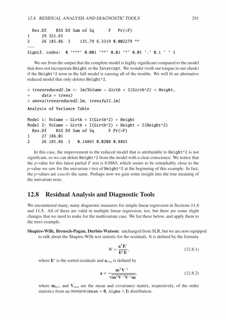
12.8. RESIDUAL ANALYSIS AND DIAGNOSTIC TOOLS 291
Res.Df RSS Df Sum of Sq F Pr(>F)
1 29 321.65
2 26 185.86 3 135.79 6.3319 0.002279 **
---
Signif. codes: 0 '***' 0.001 '**' 0.01 '*' 0.05 '.' 0.1 ' ' 1
We see from the output that the complete model is highly significant compared to the modelthat does not incorporate Height or the Intercept. We wonder (with our tongue in our cheek)if the Height^2 term in the full model is causing all of the trouble. We will fit an alternativereduced model that only deletes Height^2.
> treesreduced2.lm <- lm(Volume ~ Girth + I(Girth^2) + Height,
+ data = trees)
> anova(treesreduced2.lm, treesfull.lm)
Analysis of Variance Table
Model 1: Volume ~ Girth + I(Girth^2) + Height
Model 2: Volume ~ Girth + I(Girth^2) + Height + I(Height^2)
Res.Df RSS Df Sum of Sq F Pr(>F)
1 27 186.01
2 26 185.86 1 0.14865 0.0208 0.8865
In this case, the improvement to the reduced model that is attributable to Height^2 is notsignificant, so we can delete Height^2 from the model with a clear conscience. We notice thatthe p-value for this latest partial F test is 0.8865, which seems to be remarkably close to thep-value we saw for the univariate t test of Height^2 at the beginning of this example. In fact,the p-values are exactly the same. Perhaps now we gain some insight into the true meaning ofthe univariate tests.
12.8 Residual Analysis and Diagnostic Tools
We encountered many, many diagnostic measures for simple linear regression in Sections 11.4and 11.5. All of these are valid in multiple linear regression, too, but there are some slightchanges that we need to make for the multivariate case. We list these below, and apply them tothe trees example.
Shapiro-Wilk, Breusch-Pagan, Durbin-Watson: unchanged from SLR, but we are now equippedto talk about the Shapiro-Wilk test statistic for the residuals. It is defined by the formula
W =aTE6
ETE, (12.8.1)
where E6 is the sorted residuals and a17n is defined by
a =mTV#1
$mTV#1V#1m
, (12.8.2)
where mn71 and Vn7n are the mean and covariance matrix, respectively, of the orderstatistics from an mvnorm (mean = 0, sigma = I) distribution.
292 CHAPTER 12. MULTIPLE LINEAR REGRESSION
Leverages: are defined to be the diagonal entries of the hat matrix H (which is why we calledthem hii in Section 12.2.3). The sum of the leverages is tr(H) = p+ 1. One rule of thumbconsiders a leverage extreme if it is larger than double the mean leverage value, whichis 2(p + 1)/n, and another rule of thumb considers leverages bigger than 0.5 to indicatehigh leverage, while values between 0.3 and 0.5 indicate moderate leverage.
Standardized residuals: unchanged. Considered extreme if |Ri| > 2.
Studentized residuals: compared to a t(df = n # p # 2) distribution.
DFBETAS : The formula is generalized to
(DFBETAS ) j(i) =bj # bj(i)
S (i)$c j j
, j = 0, . . . p, i = 1, . . . , n, (12.8.3)
where c j j is the jth diagonal entry of (XTX)#1. Values larger than one for small data setsor 2/
$n for large data sets should be investigated.
DFFITS : unchanged. Larger than one in absolute value is considered extreme.
Cook’s D: compared to an f(df1 = p + 1, df2 = n # p # 1) distribution. Observations fallinghigher than the 50th percentile are extreme.
Note that plugging the value p = 1 into the formulas will recover all of the ones we saw inChapter 11.
12.9 Additional Topics
12.9.1 Nonlinear Regression
We spent the entire chapter talking about the trees data, and all of our models looked likeVolume ~Girth + Height or a variant of this model. But let us think again: we know fromelementary school that the volume of a rectangle is V = lwh and the volume of a cylinder(which is closer to what a black cherry tree looks like) is
V = &r2h or V = 4&dh, (12.9.1)
where r and d represent the radius and diameter of the tree, respectively. With this in mind, itwould seem that a more appropriate model for µ might be
µ(x1, x2) = *0x*11 x*22 , (12.9.2)
where *1 and *2 are parameters to adjust for the fact that a black cherry tree is not a perfectcylinder.
How can we fit this model? The model is not linear in the parameters any more, so ourlinear regression methods will not work. . . or will they? In the trees example we may take thelogarithm of both sides of Equation 12.9.2 to get
µ6(x1, x2) = lnRµ(x1, x2)
S= ln *0 + *1 ln x1 + *2 ln x2, (12.9.3)
and this new model µ6 is linear in the parameters *60 = ln *0, *61 = *1 and *
62 = *2. We can
use what we have learned to fit a linear model log(Volume)~log(Girth)+ log(Height),

12.9. ADDITIONAL TOPICS 293
and everything will proceed as before, with one exception: we will need to be mindful when itcomes time to make predictions because the model will have been fit on the log scale, and wewill need to transform our predictions back to the original scale (by exponentiating with exp)to make sense.
> treesNonlin.lm <- lm(log(Volume) ~ log(Girth) + log(Height),
+ data = trees)
> summary(treesNonlin.lm)
Call:
lm(formula = log(Volume) ~ log(Girth) + log(Height), data = trees)
Residuals:
Min 1Q Median 3Q Max
-0.168561 -0.048488 0.002431 0.063637 0.129223
Coefficients:
Estimate Std. Error t value Pr(>|t|)
(Intercept) -6.63162 0.79979 -8.292 5.06e-09 ***
log(Girth) 1.98265 0.07501 26.432 < 2e-16 ***
log(Height) 1.11712 0.20444 5.464 7.81e-06 ***
---
Signif. codes: 0 '***' 0.001 '**' 0.01 '*' 0.05 '.' 0.1 ' ' 1
Residual standard error: 0.08139 on 28 degrees of freedom
Multiple R-squared: 0.9777, Adjusted R-squared: 0.9761
F-statistic: 613.2 on 2 and 28 DF, p-value: < 2.2e-16
This is our best model yet (judging by R2 and R2), all of the parameters are significant, it is
simpler than the quadratic or interaction models, and it even makes theoretical sense. It rarelygets any better than that.
We may get confidence intervals for the parameters, but remember that it is usually betterto transform back to the original scale for interpretation purposes :
> exp(confint(treesNonlin.lm))
2.5 % 97.5 %
(Intercept) 0.0002561078 0.006783093
log(Girth) 6.2276411645 8.468066317
log(Height) 2.0104387829 4.645475188
(Note that we did not update the row labels of the matrix to show that we exponentiated andso they are misleading as written.) We do predictions just as before. Remember to transformthe response variable back to the original scale after prediction.
> new <- data.frame(Girth = c(9.1, 11.6, 12.5), Height = c(69,
+ 74, 87))
> exp(predict(treesNonlin.lm, newdata = new, interval = "confidence"))
294 CHAPTER 12. MULTIPLE LINEAR REGRESSION
fit lwr upr
1 11.90117 11.25908 12.57989
2 20.82261 20.14652 21.52139
3 28.93317 27.03755 30.96169
The predictions and intervals are slightly di!erent from those calculated earlier, but theyare close. Note that we did not need to transform the Girth and Height arguments in thedataframe new. All transformations are done for us automatically.
12.9.2 Real Nonlinear Regression
We saw with the trees data that a nonlinear model might be more appropriate for the databased on theoretical considerations, and we were lucky because the functional form of µ al-lowed us to take logarithms to transform the nonlinear model to a linear one. The same trickwill not work in other circumstances, however. We need techniques to fit general models of theform
Y = µ(X) + $, (12.9.4)
where µ is some crazy function that does not lend itself to linear transformations.There are a host of methods to address problems like these which are studied in advanced
regression classes. The interested reader should see Neter et al [67] or Tabachnick and Fidell[83].
It turns out that John Fox has posted an Appendix to his book [29] which discusses someof the methods and issues associated with nonlinear regression; see
http://cran.r-project.org/doc/contrib/Fox-Companion/appendix.html
12.9.3 Multicollinearity
A multiple regression model exhibits multicollinearity when two or more of the explanatoryvariables are substantially correlated with each other. We can measure multicollinearity byhaving one of the explanatory play the role of “dependent variable” and regress it on the re-maining explanatory variables. The the R2 of the resulting model is near one, then we say thatthe model is multicollinear or shows multicollinearity.
Multicollinearity is a problem because it causes instability in the regression model. Theinstability is a consequence of redundancy in the explanatory variables: a high R2 indicates astrong dependence between the selected independent variable and the others. The redundantinformation inflates the variance of the parameter estimates which can cause them to be statis-tically insignificant when they would have been significant otherwise. To wit, multicollinearityis usually measured by what are called variance inflation factors.
Once multicollinearity has been diagnosed there are several approaches to remediate it.Here are a couple of important ones.
Principal Components Analysis. This approach casts out two or more of the original explana-tory variables and replaces them with new variables, derived from the original ones, thatare by design uncorrelated with one another. The redundancy is thus eliminated and wemay proceed as usual with the new variables in hand. Principal Components Analysis isimportant for other reasons, too, not just for fixing multicollinearity problems.

12.9. ADDITIONAL TOPICS 295
Ridge Regression. The idea of this approach is to replace the original parameter estimateswith a di!erent type of parameter estimate which is more stable under multicollinearity.The estimators are not found by ordinary least squares but rather a di!erent optimizationprocedure which incorporates the variance inflation factor information.
We decided to omit a thorough discussion of multicollinearity because we are not equipped tohandle the mathematical details. Perhaps the topic will receive more attention in a later edition.
• What to do when data are not normal
* Bootstrap (see Chapter 13).
12.9.4 Akaike’s Information Criterion
AIC = #2 ln L + 2(p + 1)

296 CHAPTER 12. MULTIPLE LINEAR REGRESSION
Chapter Exercises
Exercise 12.1. Use Equations 12.3.1, 12.3.2, and 12.3.3 to prove the Anova Equality:
S S TO = S S E + S SR.
Chapter 13
Resampling Methods
Computers have changed the face of statistics. Their quick computational speed and flawlessaccuracy, coupled with large data sets acquired by the researcher, make them indispensable formany modern analyses. In particular, resampling methods (due in large part to Bradley Efron)have gained prominence in the modern statistician’s repertoire. We first look at a classicalproblem to get some insight why.
I have seen Statistical Computing with R by Rizzo [71] and I recommend it to those lookingfor a more advanced treatment with additional topics. I believe that Monte Carlo Statistical
Methods by Robert and Casella [72] has a new edition that integrates R into the narrative.
What do I want them to know?
• basic philosophy of resampling and why it is important
• resampling for standard errors and confidence intervals
• resampling for hypothesis tests (permutation tests)
13.1 Introduction
Classical question Given a population of interest, how may we e!ectively learn some of itssalient features, e.g., the population’s mean? One way is through representative randomsampling. Given a random sample, we summarize the information contained therein bycalculating a reasonable statistic, e.g., the sample mean. Given a value of a statistic, howdo we know whether that value is significantly di!erent from that which was expected?We don’t; we look at the sampling distribution of the statistic, and we try to make prob-abilistic assertions based on a confidence level or other consideration. For example, wemay find ourselves saying things like, "With 95% confidence, the true population meanis greater than zero."
Problem Unfortunately, in most cases the sampling distribution is unknown. Thus, in thepast, in e!orts to say something useful, statisticians have been obligated to place somerestrictive assumptions on the underlying population. For example, if we suppose thatthe population has a normal distribution, then we can say that the distribution of X isnormal, too, with the same mean (and a smaller standard deviation). It is then easy todraw conclusions, make inferences, and go on about our business.
297
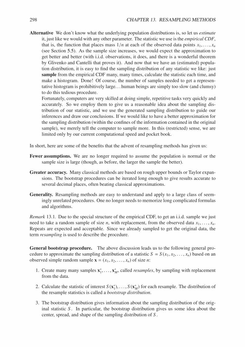
298 CHAPTER 13. RESAMPLING METHODS
Alternative We don’t know what the underlying population distributions is, so let us estimateit, just like we would with any other parameter. The statistic we use is the empirical CDF,that is, the function that places mass 1/n at each of the observed data points x1, . . . , xn(see Section 5.5). As the sample size increases, we would expect the approximation toget better and better (with i.i.d. observations, it does, and there is a wonderful theoremby Glivenko and Cantelli that proves it). And now that we have an (estimated) popula-tion distribution, it is easy to find the sampling distribution of any statistic we like: justsample from the empirical CDF many, many times, calculate the statistic each time, andmake a histogram. Done! Of course, the number of samples needed to get a represen-tative histogram is prohibitively large. . . human beings are simply too slow (and clumsy)to do this tedious procedure.Fortunately, computers are very skilled at doing simple, repetitive tasks very quickly andaccurately. So we employ them to give us a reasonable idea about the sampling dis-tribution of our statistic, and we use the generated sampling distribution to guide ourinferences and draw our conclusions. If we would like to have a better approximation forthe sampling distribution (within the confines of the information contained in the originalsample), we merely tell the computer to sample more. In this (restricted) sense, we arelimited only by our current computational speed and pocket book.
In short, here are some of the benefits that the advent of resampling methods has given us:
Fewer assumptions. We are no longer required to assume the population is normal or thesample size is large (though, as before, the larger the sample the better).
Greater accuracy. Many classical methods are based on rough upper bounds or Taylor expan-sions. The bootstrap procedures can be iterated long enough to give results accurate toseveral decimal places, often beating classical approximations.
Generality. Resampling methods are easy to understand and apply to a large class of seem-ingly unrelated procedures. One no longer needs to memorize long complicated formulasand algorithms.
Remark 13.1. Due to the special structure of the empirical CDF, to get an i.i.d. sample we justneed to take a random sample of size n, with replacement, from the observed data x1, . . . , xn.Repeats are expected and acceptable. Since we already sampled to get the original data, theterm resampling is used to describe the procedure.
General bootstrap procedure. The above discussion leads us to the following general pro-cedure to approximate the sampling distribution of a statistic S = S (x1, x2, . . . , xn) based on anobserved simple random sample x = (x1, x2, . . . , xn) of size n:
1. Create many many samples x61, . . . , x6M, called resamples, by sampling with replacement
from the data.
2. Calculate the statistic of interest S (x61), . . . , S (x6M) for each resample. The distribution of
the resample statistics is called a bootstrap distribution.
3. The bootstrap distribution gives information about the sampling distribution of the orig-inal statistic S . In particular, the bootstrap distribution gives us some idea about thecenter, spread, and shape of the sampling distribution of S .
13.2. BOOTSTRAP STANDARD ERRORS 299
13.2 Bootstrap Standard Errors
Since the bootstrap distribution gives us information about a statistic’s sampling distribution,we can use the bootstrap distribution to estimate properties of the statistic. We will illustratethe bootstrap procedure in the special case that the statistic S is a standard error.
Example 13.2. Standard error of the mean. In this example we illustrate the bootstrap byestimating the standard error of the sample meanand we will do it in the special case that theunderlying population is norm(mean = 3, sd = 1).
Of course, we do not really need a bootstrap distribution here because from Section 8.2 weknow that X 4 norm(mean = 3, sd = 1/
$n), but we proceed anyway to investigate how the
bootstrap performs when we know what the answer should be ahead of time.We will take a random sample of size n = 25 from the population. Then we will resample
the data 1000 times to get 1000 resamples of size 25. We will calculate the sample mean ofeach of the resamples, and will study the data distribution of the 1000 values of x.
> srs <- rnorm(25, mean = 3)
> resamps <- replicate(1000, sample(srs, 25, TRUE), simplify = FALSE)
> xbarstar <- sapply(resamps, mean, simplify = TRUE)
A histogram of the 1000 values of x is shown in Figure 13.2.1, and was produced by thefollowing code.
> hist(xbarstar, breaks = 40, prob = TRUE)
> curve(dnorm(x, 3, 0.2), add = TRUE) # overlay true normal density
We have overlain what we know to be the true sampling distribution of X, namely, anorm(mean = 3, sd = 1/
$25) distribution. The histogram matches the true sampling distribu-
tion pretty well with respect to shape and spread. . . but notice how the histogram is o!-centera little bit. This is not a coincidence – in fact, it can be shown that the mean of the bootstrapdistribution is exactly the mean of the original sample, that is, the value of the statistic that weoriginally observed. Let us calculate the mean of the bootstrap distribution and compare it tothe mean of the original sample:
> mean(xbarstar)
[1] 2.711477
> mean(srs)
[1] 2.712087
> mean(xbarstar) - mean(srs)
[1] -0.0006096438
Notice how close the two values are. The di!erence between them is an estimate of howbiased the original statistic is, the so-called bootstrap estimate of bias. Since the estimate is sosmall we would expect our original statistic (X) to have small bias, but this is no surprise to usbecause we already knew from Section 8.1.1 that X is an unbiased estimator of the populationmean.
Now back to our original problem, we would like to estimate the standard error of X. Look-ing at the histogram, we see that the spread of the bootstrap distribution is similar to the spreadof the sampling distribution. Therefore, it stands to reason that we could estimate the standarderror of X with the sample standard deviation of the resample statistics. Let us try and see.
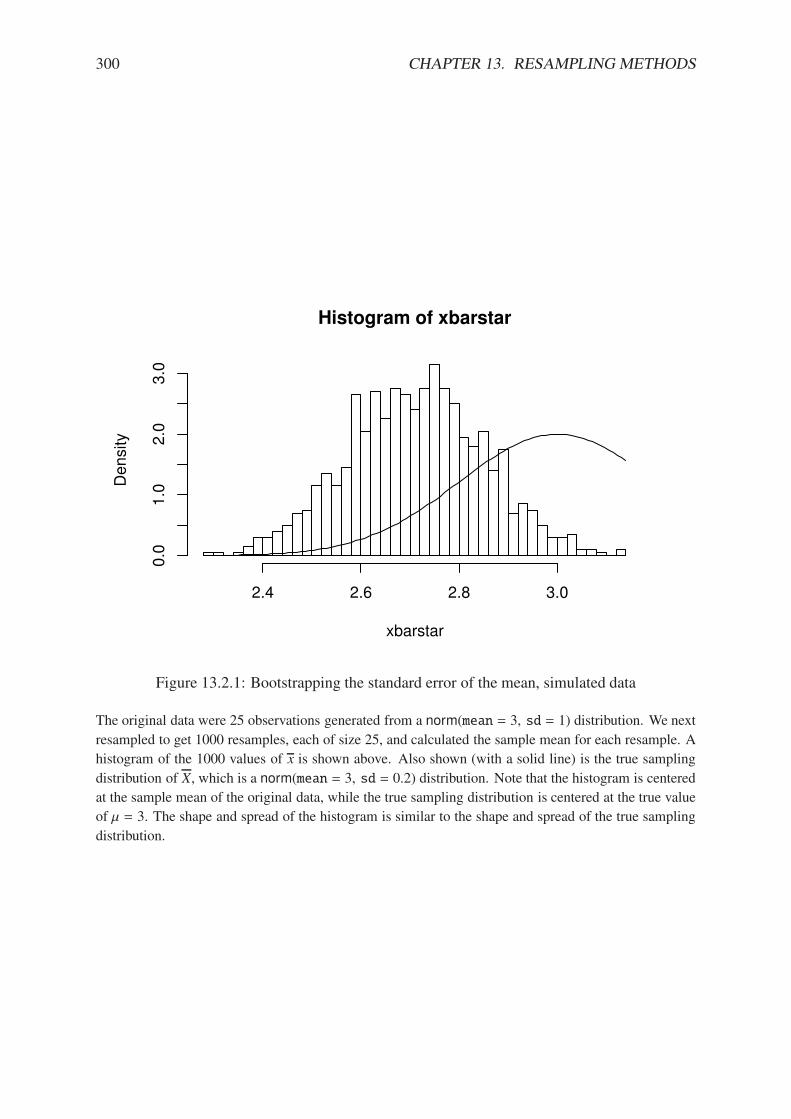
300 CHAPTER 13. RESAMPLING METHODS
Histogram of xbarstar
xbarstar
Densi
ty
2.4 2.6 2.8 3.0
0.0
1.0
2.0
3.0
Figure 13.2.1: Bootstrapping the standard error of the mean, simulated data
The original data were 25 observations generated from a norm(mean = 3, sd = 1) distribution. We next
resampled to get 1000 resamples, each of size 25, and calculated the sample mean for each resample. A
histogram of the 1000 values of x is shown above. Also shown (with a solid line) is the true sampling
distribution of X, which is a norm(mean = 3, sd = 0.2) distribution. Note that the histogram is centered
at the sample mean of the original data, while the true sampling distribution is centered at the true value
of µ = 3. The shape and spread of the histogram is similar to the shape and spread of the true sampling
distribution.
13.2. BOOTSTRAP STANDARD ERRORS 301
> sd(xbarstar)
[1] 0.1390366
We know from theory that the true standard error is 1/$25 = 0.20. Our bootstrap estimate
is not very far from the theoretical value.
Remark 13.3. What would happen if we take more resamples? Instead of 1000 resamples, wecould increase to, say, 2000, 3000, or even 4000. . . would it help? The answer is both yes andno. Keep in mind that with resampling methods there are two sources of randomness: thatfrom the original sample, and that from the subsequent resampling procedure. An increasednumber of resamples would reduce the variation due to the second part, but would do nothingto reduce the variation due to the first part. We only took an original sample of size n = 25, andresampling more and more would never generate more information about the population thanwas already there. In this sense, the statistician is limited by the information contained in theoriginal sample.
Example 13.4. Standard error of the median. We look at one where we do not know theanswer ahead of time. This example uses the rivers data set. Recall the stemplot on pageon page 41 that we made for these data which shows them to be markedly right-skewed, so anatural estimate of center would be the sample median. Unfortunately, its sampling distributionfalls out of our reach. We use the bootstrap to help us with this problem, and the modificationsto the last example are trivial.
> resamps <- replicate(1000, sample(rivers, 141, TRUE), simplify = FALSE)
> medstar <- sapply(resamps, median, simplify = TRUE)
> sd(medstar)
[1] 27.21154
The graph is shown in Figure 13.2.2, and was produced by the following code.
> hist(medstar, breaks = 40, prob = TRUE)
> median(rivers)
[1] 425
> mean(medstar)
[1] 427.88
> mean(medstar) - median(rivers)
[1] 2.88
Example 13.5. The boot package in R. It turns out that there are many bootstrap proceduresand commands already built into base R, in the boot package. Further, inside the boot packagethere is even a function called boot. The basic syntax is of the form:
boot(data, statistic , R)
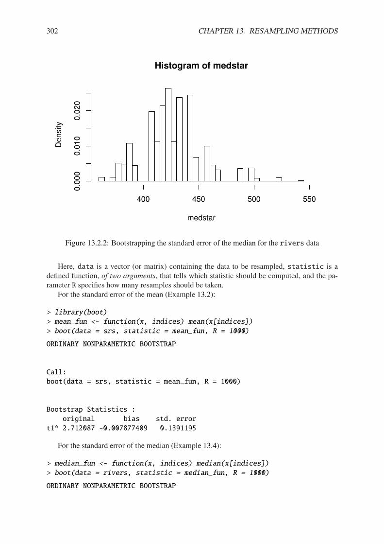
302 CHAPTER 13. RESAMPLING METHODS
Histogram of medstar
medstar
Densi
ty
400 450 500 550
0.0
00
0.0
10
0.0
20
Figure 13.2.2: Bootstrapping the standard error of the median for the rivers data
Here, data is a vector (or matrix) containing the data to be resampled, statistic is adefined function, of two arguments, that tells which statistic should be computed, and the pa-rameter R specifies how many resamples should be taken.
For the standard error of the mean (Example 13.2):
> library(boot)
> mean_fun <- function(x, indices) mean(x[indices])
> boot(data = srs, statistic = mean_fun, R = 1000)
ORDINARY NONPARAMETRIC BOOTSTRAP
Call:
boot(data = srs, statistic = mean_fun, R = 1000)
Bootstrap Statistics :
original bias std. error
t1* 2.712087 -0.007877409 0.1391195
For the standard error of the median (Example 13.4):
> median_fun <- function(x, indices) median(x[indices])
> boot(data = rivers, statistic = median_fun, R = 1000)
ORDINARY NONPARAMETRIC BOOTSTRAP
13.3. BOOTSTRAP CONFIDENCE INTERVALS 303
Call:
boot(data = rivers, statistic = median_fun, R = 1000)
Bootstrap Statistics :
original bias std. error
t1* 425 2.456 25.63723
We notice that the output from both methods of estimating the standard errors producedsimilar results. In fact, the boot procedure is to be preferred since it invisibly returns muchmore information (which we will use later) than our naive script and it is much quicker in itscomputations.
Remark 13.6. Some things to keep in mind about the bootstrap:
• For many statistics, the bootstrap distribution closely resembles the sampling distributionwith respect to spread and shape. However, the bootstrap will not have the same centeras the true sampling distribution. While the sampling distribution is centered at the pop-ulation mean (plus any bias), the bootstrap distribution is centered at the original valueof the statistic (plus any bias). The boot function gives an empirical estimate of the biasof the statistic as part of its output.
• We tried to estimate the standard error, but we could have (in principle) tried to esti-mate something else. Note from the previous remark, however, that it would be uselessto estimate the population mean µ using the bootstrap since the mean of the bootstrapdistribution is the observed x.
• You don’t get something from nothing. We have seen that we can take a random samplefrom a population and use bootstrap methods to get a very good idea about standarderrors, bias, and the like. However, one must not get lured into believing that by doingsome random resampling somehow one gets more information about the parameters thanthat which was contained in the original sample. Indeed, there is some uncertainty aboutthe parameter due to the randomness of the original sample, and there is even moreuncertainty introduced by resampling. One should think of the bootstrap as just anotherestimation method, nothing more, nothing less.
13.3 Bootstrap Confidence Intervals
13.3.1 Percentile Confidence Intervals
As a first try, we want to obtain a 95% confidence interval for a parameter. Typically thestatistic we use to estimate the parameter is centered at (or at least close by) the parameter; insuch cases a 95% confidence interval for the parameter is nothing more than a 95% confidenceinterval for the statistic. And to find a 95% confidence interval for the statistic we need only goto its sampling distribution to find an interval that contains 95% of the area. (The most popularchoice is the equal-tailed interval with 2.5% in each tail.)
This is incredibly easy to accomplish with the bootstrap. We need only to take a bunch ofbootstrap resamples, order them, and choose the (/2th and (1 # ()th percentiles. There is afunction boot.ci in R already created to do just this. Note that in order to use the function
304 CHAPTER 13. RESAMPLING METHODS
boot.ci we must first run the boot function and save the output in a variable, for example,data.boot. We then plug data.boot into the function boot.ci.
Example 13.7. Percentile interval for the expected value of the median. Wee will try thenaive approach where we generate the resamples and calculate the percentile interval by hand.
> btsamps <- replicate(2000, sample(stack.loss, 21, TRUE),
+ simplify = FALSE)
> thetast <- sapply(btsamps, median, simplify = TRUE)
> mean(thetast)
[1] 14.794
> median(stack.loss)
[1] 15
> quantile(thetast, c(0.025, 0.975))
2.5% 97.5%
12 18
Example 13.8. Confidence interval for expected value of the median, 2nd try. Now we willdo it the right way with the boot function.
> library(boot)
> med_fun <- function(x, ind) median(x[ind])
> med_boot <- boot(stack.loss, med_fun, R = 2000)
> boot.ci(med_boot, type = c("perc", "norm", "bca"))
BOOTSTRAP CONFIDENCE INTERVAL CALCULATIONS
Based on 2000 bootstrap replicates
CALL :
boot.ci(boot.out = med_boot, type = c("perc", "norm", "bca"))
Intervals :
Level Normal Percentile BCa
95% (12.11, 18.34 ) (12.00, 18.00 ) (11.00, 18.00 )
Calculations and Intervals on Original Scale
13.3.2 Student’s t intervals (“normal intervals”)
The idea is to use confidence intervals that we already know and let the bootstrap help us whenwe get into trouble. We know that a 100(1#()% confidence interval for the mean of a SRS (n)from a normal distribution is
X ± t(/2(df = n # 1)S$n, (13.3.1)
where t(/2(df = n # 1) is the appropriate critical value from Student’s t distribution, and weremember that an estimate for the standard error of X is S/
$n. Of course, the estimate for the
standard error will change when the underlying population distribution is not normal, or when
13.4. RESAMPLING IN HYPOTHESIS TESTS 305
we use a statistic more complicated than X. In those situations the bootstrap will give us quitereasonable estimates for the standard error. And as long as the sampling distribution of ourstatistic is approximately bell-shaped with small bias, the interval
statistic ± t(/2(df = n # 1) 6 SE(statistic) (13.3.2)
will have approximately 100(1 # ()% confidence of containing IE(statistic).
Example 13.9. We will use the t-interval method to find the bootstrap CI for the median. Wehave looked at the bootstrap distribution; it appears to be symmetric and approximately moundshaped. Further, we may check that the bias is approximately 40, which on the scale of thesedata is practically negligible. Thus, we may consider looking at the t-intervals. Note that, sinceour sample is so large, instead of t-intervals we will essentially be using z-intervals.
Please see the handout, “Bootstrapping Confidence Intervals for the Median, 3rd try.”We see that, considering the scale of the data, the confidence intervals compare with each
other quite well.
Remark 13.10. We have seen two methods for bootstrapping confidence intervals for a statistic.Which method should we use? If the bias of the bootstrap distribution is small and if thedistribution is close to normal, then the percentile and t-intervals will closely agree. If theintervals are noticeably di!erent, then it should be considered evidence that the normality andbias conditions are not met. In this case, neither interval should be used.
• BCa: bias-corrected and accelerated
* transformation invariant
* more correct and accurate
* not monotone in coverage level?
• t - intervals
* more natural
* numerically unstable
• Can do things like transform scales, compute confidence intervals, and then transformback.
• Studentized bootstrap confidence intervals where is the Studentized version of is the orderstatistic of the simulation
13.4 Resampling in Hypothesis Tests
The classical two-sample problem can be stated as follows: given two groups of interest, wewould like to know whether these two groups are significantly di!erent from one another orwhether the groups are reasonably similar. The standard way to decide is to
1. Go collect some information from the two groups and calculate an associated statistic,for example, X1 # X2.

306 CHAPTER 13. RESAMPLING METHODS
2. Suppose that there is no di!erence in the groups, and find the distribution of the statisticin 1.
3. Locate the observed value of the statistic with respect to the distribution found in 2. Avalue in the main body of the distribution is not spectacular, it could reasonably haveoccurred by chance. A value in the tail of the distribution is unlikely, and hence providesevidence against the null hypothesis that the population distributions are the same.
Of course, we usually compute a p-value, defined to be the probability of the observed valueof the statistic or more extreme when the null hypothesis is true. Small p-values are evidenceagainst the null hypothesis. It is not immediately obvious how to use resampling methods here,so we discuss an example.
Example 13.11. A study concerned di!ering dosages of the antiretroviral drug AZT. The com-mon dosage is 300mg daily. Higher doses cause more side a!ects, but are they significantlyhigher? We examine for a 600mg dose. The data are as follows: We compare the scores fromthe two groups by computing the di!erence in their sample means. The 300mg data wereentered in x1 and the 600mg data were entered into x2. The observed di!erence was
300 mg 284 279 289 292 287 295 285 279 306 298600 mg 298 307 297 279 291 335 299 300 306 291
The average amounts can be found:> mean(x1)
[1] 289.4
> mean(x2)
[1] 300.3
with an observed di!erence of mean(x2) - mean(x1) = 10.9. As expected, the 600mg measurements seem to have a higher average, and we might be interested in trying todecide if the average amounts are significantly di!erent. The null hypothesis should be thatthere is no di!erence in the amounts, that is, the groups are more or less the same. If the nullhypothesis were true, then the two groups would indeed be the same, or just one big group. Inthat case, the observed di!erence in the sample means just reflects the random assignment intothe arbitrary x1 and x2 categories. It is now clear how we may resample, consistent with thenull hypothesis.
Procedure:
1. Randomly resample 10 scores from the combined scores of x1 and x2, and assign thento the “x1” group. The rest will then be in the “x2” group. Calculate the di!erence in(re)sampled means, and store that value.
2. Repeat this procedure many, many times and draw a histogram of the resampled statistics,called the permutation distribution. Locate the observed di!erence 10.9 on the histogramto get the p-value. If the p-value is small, then we consider that evidence against thehypothesis that the groups are the same.
Remark 13.12. In calculating the permutation test p-value, the formula is essentially the pro-portion of resample statistics that are greater than or equal to the observed value. Of course,this is merely an estimate of the true p-value. As it turns out, an adjustment of +1 to boththe numerator and denominator of the proportion improves the performance of the estimatedp-value, and this adjustment is implemented in the ts.perm function.
13.4. RESAMPLING IN HYPOTHESIS TESTS 307
> library(coin)
> oneway_test(len ~ supp, data = ToothGrowth)
Asymptotic 2-Sample Permutation Test
data: len by supp (OJ, VC)
Z = 1.8734, p-value = 0.06102
alternative hypothesis: true mu is not equal to 0
13.4.1 Comparison with the Two Sample t test
We know from Chapter 10 to use the two-sample t-test to tell whether there is an improvementas a result of taking the intervention class. Note that the t-test assumes normal underlyingpopulations, with unknown variance, and small sample n = 10. What does the t-test say?Below is the output.
> t.test(len ~ supp, data = ToothGrowth, alt = "greater", var.equal = TRUE)
Two Sample t-test
data: len by supp
t = 1.9153, df = 58, p-value = 0.03020
alternative hypothesis: true difference in means is greater than 0
95 percent confidence interval:
0.4708204 Inf
sample estimates:
mean in group OJ mean in group VC
20.66333 16.96333
The p-value for the t-test was 0.03, while the permutation test p-value was 0.061. Note thatthere is an underlying normality assumption for the t-test, which isn’t present in the permutationtest. If the normality assumption may be questionable, then the permutation test would be morereasonable. We see what can happen when using a test in a situation where the assumptionsare not met: smaller p-values. In situations where the normality assumptions are not met,for example, small sample scenarios, the permutation test is to be preferred. In particular, ifaccuracy is very important then we should use the permutation test.
Remark 13.13. Here are some things about permutation tests to keep in mind.
• While the permutation test does not require normality of the populations (as contrastedwith the t-test), nevertheless it still requires that the two groups are exchangeable; seeSection 7.5. In particular, this means that they must be identically distributed under thenull hypothesis. They must have not only the same means, but they must also have thesame spread, shape, and everything else. This assumption may or may not be true ina given example, but it will rarely cause the t-test to outperform the permutation test,because even if the sample standard deviations are markedly di!erent it does not meanthat the population standard deviations are di!erent. In many situations the permutationtest will also carry over to the t-test.
• If the distribution of the groups is close to normal, then the t-test p-value and the boot-strap p-value will be approximately equal. If they di!er markedly, then this should beconsidered evidence that the normality assumptions do not hold.

308 CHAPTER 13. RESAMPLING METHODS
• The generality of the permutation test is such that one can use all kinds of statistics tocompare the two groups. One could compare the di!erence in variances or the di!erencein (just about anything). Alternatively, one could compare the ratio of sample means,X1/X2. Of course, under the null hypothesis this last quantity should be near 1.
• Just as with the bootstrap, the answer we get is subject to variability due to the inherentrandomness of resampling from the data. We can make the variability as small as we likeby taking su"ciently many resamples. How many? If the conclusion is very important(that is, if lots of money is at stake), then take thousands. For point estimation problemstypically, R = 1000 resamples, or so, is enough. In general, if the true p-value is p thenthe standard error of the estimated p-value is
Np(1 # p)/R. You can choose R to get
whatever accuracy desired.
• Other possible testing designs:
* Matched Pairs Designs.
* Relationship between two variables.

13.4. RESAMPLING IN HYPOTHESIS TESTS 309
Chapter Exercises

310 CHAPTER 13. RESAMPLING METHODS

Chapter 14
Categorical Data Analysis
This chapter is still under substantial revision. At any time you can preview any released draftswith the development version of the IPSUR package which is available from R-Forge:
> install.packages("IPSUR", repos = "http://R-Forge.R-project.org")
> library(IPSUR)
> read(IPSUR)
311

312 CHAPTER 14. CATEGORICAL DATA ANALYSIS

Chapter 15
Nonparametric Statistics
This chapter is still under substantial revision. At any time you can preview any released draftswith the development version of the IPSUR package which is available from R-Forge:
> install.packages("IPSUR", repos = "http://R-Forge.R-project.org")
> library(IPSUR)
> read(IPSUR)
313

314 CHAPTER 15. NONPARAMETRIC STATISTICS

Chapter 16
Time Series
This chapter is still under substantial revision. At any time you can preview any released draftswith the development version of the IPSUR package which is available from R-Forge:
> install.packages("IPSUR", repos = "http://R-Forge.R-project.org")
> library(IPSUR)
> read(IPSUR)
315

316 CHAPTER 16. TIME SERIES
Appendix A
R Session Information
If you ever write the R help mailing list with a question, then you should include your sessioninformation in the email; it makes the reader’s job easier and is requested by the Posting Guide.Here is how to do that, and below is what the output looks like.
> sessionInfo()
R version 2.11.1 (2010-05-31)
x86_64-pc-linux-gnu
locale:
[1] LC_CTYPE=en_US.UTF-8 LC_NUMERIC=C
[3] LC_TIME=en_US.UTF-8 LC_COLLATE=en_US.UTF-8
[5] LC_MONETARY=C LC_MESSAGES=en_US.UTF-8
[7] LC_PAPER=en_US.UTF-8 LC_NAME=C
[9] LC_ADDRESS=C LC_TELEPHONE=C
[11] LC_MEASUREMENT=en_US.UTF-8 LC_IDENTIFICATION=C
attached base packages:
[1] splines grid stats4 tcltk stats graphics grDevices
[8] utils datasets methods base
other attached packages:
[1] coin_1.0-12 modeltools_0.2-16
[3] boot_1.2-42 scatterplot3d_0.3-30
[5] lmtest_0.9-26 zoo_1.6-4
[7] reshape_0.8.3 plyr_1.0.3
[9] Hmisc_3.8-2 HH_2.1-32
[11] leaps_2.9 multcomp_1.1-7
[13] survival_2.35-8 TeachingDemos_2.6
[15] mvtnorm_0.9-92 distrEx_2.2
[17] actuar_1.1-0 evd_2.2-4
[19] distr_2.2.3 sfsmisc_1.0-11
[21] startupmsg_0.7 combinat_0.0-7
[23] prob_0.9-2 lattice_0.18-8
[25] e1071_1.5-24 class_7.3-2
[27] qcc_2.0.1 aplpack_1.2.3
317

318 APPENDIX A. R SESSION INFORMATION
[29] RcmdrPlugin.IPSUR_0.1-7 Rcmdr_1.5-6
[31] car_1.2-16
loaded via a namespace (and not attached):
[1] cluster_1.13.1 tools_2.11.1

Appendix B
GNU Free Documentation License
Version 1.3, 3 November 2008
Copyright (C) 2000, 2001, 2002, 2007, 2008 Free Software Foundation, Inc.
http://fsf.org/
Everyone is permitted to copy and distribute verbatim copies of this license document, butchanging it is not allowed.
0. PREAMBLE
The purpose of this License is to make a manual, textbook, or other functional and useful doc-ument "free" in the sense of freedom: to assure everyone the e!ective freedom to copy andredistribute it, with or without modifying it, either commercially or noncommercially. Secon-darily, this License preserves for the author and publisher a way to get credit for their work,while not being considered responsible for modifications made by others.
This License is a kind of "copyleft", which means that derivative works of the documentmust themselves be free in the same sense. It complements the GNU General Public License,which is a copyleft license designed for free software.
We have designed this License in order to use it for manuals for free software, because freesoftware needs free documentation: a free program should come with manuals providing thesame freedoms that the software does. But this License is not limited to software manuals; itcan be used for any textual work, regardless of subject matter or whether it is published as aprinted book. We recommend this License principally for works whose purpose is instructionor reference.
1. APPLICABILITY AND DEFINITIONS
This License applies to any manual or other work, in any medium, that contains a notice placedby the copyright holder saying it can be distributed under the terms of this License. Such anotice grants a world-wide, royalty-free license, unlimited in duration, to use that work underthe conditions stated herein. The "Document", below, refers to any such manual or work. Anymember of the public is a licensee, and is addressed as "you". You accept the license if youcopy, modify or distribute the work in a way requiring permission under copyright law.
319

320 APPENDIX B. GNU FREE DOCUMENTATION LICENSE
A "Modified Version" of the Document means any work containing the Document or a por-tion of it, either copied verbatim, or with modifications and/or translated into another language.
A "Secondary Section" is a named appendix or a front-matter section of the Documentthat deals exclusively with the relationship of the publishers or authors of the Document to theDocument’s overall subject (or to related matters) and contains nothing that could fall directlywithin that overall subject. (Thus, if the Document is in part a textbook of mathematics, aSecondary Section may not explain any mathematics.) The relationship could be a matter ofhistorical connection with the subject or with related matters, or of legal, commercial, philo-sophical, ethical or political position regarding them.
The "Invariant Sections" are certain Secondary Sections whose titles are designated, asbeing those of Invariant Sections, in the notice that says that the Document is released under thisLicense. If a section does not fit the above definition of Secondary then it is not allowed to bedesignated as Invariant. The Document may contain zero Invariant Sections. If the Documentdoes not identify any Invariant Sections then there are none.
The "Cover Texts" are certain short passages of text that are listed, as Front-Cover Texts orBack-Cover Texts, in the notice that says that the Document is released under this License. AFront-Cover Text may be at most 5 words, and a Back-Cover Text may be at most 25 words.
A "Transparent" copy of the Document means a machine-readable copy, represented in aformat whose specification is available to the general public, that is suitable for revising the doc-ument straightforwardly with generic text editors or (for images composed of pixels) genericpaint programs or (for drawings) some widely available drawing editor, and that is suitable forinput to text formatters or for automatic translation to a variety of formats suitable for inputto text formatters. A copy made in an otherwise Transparent file format whose markup, or ab-sence of markup, has been arranged to thwart or discourage subsequent modification by readersis not Transparent. An image format is not Transparent if used for any substantial amount oftext. A copy that is not "Transparent" is called "Opaque".
Examples of suitable formats for Transparent copies include plain ASCII without markup,Texinfo input format, LATEX input format, SGML or XML using a publicly available DTD,and standard-conforming simple HTML, PostScript or PDF designed for human modification.Examples of transparent image formats include PNG, XCF and JPG. Opaque formats includeproprietary formats that can be read and edited only by proprietary word processors, SGML orXML for which the DTD and/or processing tools are not generally available, and the machine-generated HTML, PostScript or PDF produced by some word processors for output purposesonly.
The "Title Page" means, for a printed book, the title page itself, plus such following pagesas are needed to hold, legibly, the material this License requires to appear in the title page. Forworks in formats which do not have any title page as such, "Title Page" means the text near themost prominent appearance of the work’s title, preceding the beginning of the body of the text.
The "publisher" means any person or entity that distributes copies of the Document to thepublic.
A section "Entitled XYZ" means a named subunit of the Document whose title either isprecisely XYZ or contains XYZ in parentheses following text that translates XYZ in anotherlanguage. (Here XYZ stands for a specific section name mentioned below, such as "Acknowl-edgements", "Dedications", "Endorsements", or "History".) To "Preserve the Title" of such asection when you modify the Document means that it remains a section "Entitled XYZ" ac-cording to this definition.
The Document may include Warranty Disclaimers next to the notice which states that thisLicense applies to the Document. These Warranty Disclaimers are considered to be included by
321
reference in this License, but only as regards disclaiming warranties: any other implication thatthese Warranty Disclaimers may have is void and has no e!ect on the meaning of this License.
2. VERBATIM COPYING
You may copy and distribute the Document in any medium, either commercially or noncom-mercially, provided that this License, the copyright notices, and the license notice saying thisLicense applies to the Document are reproduced in all copies, and that you add no other con-ditions whatsoever to those of this License. You may not use technical measures to obstruct orcontrol the reading or further copying of the copies you make or distribute. However, you mayaccept compensation in exchange for copies. If you distribute a large enough number of copiesyou must also follow the conditions in section 3.
You may also lend copies, under the same conditions stated above, and you may publiclydisplay copies.
3. COPYING IN QUANTITY
If you publish printed copies (or copies in media that commonly have printed covers) of theDocument, numbering more than 100, and the Document’s license notice requires Cover Texts,you must enclose the copies in covers that carry, clearly and legibly, all these Cover Texts:Front-Cover Texts on the front cover, and Back-Cover Texts on the back cover. Both coversmust also clearly and legibly identify you as the publisher of these copies. The front covermust present the full title with all words of the title equally prominent and visible. You mayadd other material on the covers in addition. Copying with changes limited to the covers, aslong as they preserve the title of the Document and satisfy these conditions, can be treated asverbatim copying in other respects.
If the required texts for either cover are too voluminous to fit legibly, you should put the firstones listed (as many as fit reasonably) on the actual cover, and continue the rest onto adjacentpages.
If you publish or distribute Opaque copies of the Document numbering more than 100,you must either include a machine-readable Transparent copy along with each Opaque copy,or state in or with each Opaque copy a computer-network location from which the generalnetwork-using public has access to download using public-standard network protocols a com-plete Transparent copy of the Document, free of added material. If you use the latter option,you must take reasonably prudent steps, when you begin distribution of Opaque copies in quan-tity, to ensure that this Transparent copy will remain thus accessible at the stated location untilat least one year after the last time you distribute an Opaque copy (directly or through youragents or retailers) of that edition to the public.
It is requested, but not required, that you contact the authors of the Document well beforeredistributing any large number of copies, to give them a chance to provide you with an updatedversion of the Document.
4. MODIFICATIONS
You may copy and distribute a Modified Version of the Document under the conditions ofsections 2 and 3 above, provided that you release the Modified Version under precisely this

322 APPENDIX B. GNU FREE DOCUMENTATION LICENSE
License, with the Modified Version filling the role of the Document, thus licensing distributionand modification of the Modified Version to whoever possesses a copy of it. In addition, youmust do these things in the Modified Version:
A. Use in the Title Page (and on the covers, if any) a title distinct from that of the Document,and from those of previous versions (which should, if there were any, be listed in the Historysection of the Document). You may use the same title as a previous version if the originalpublisher of that version gives permission.
B. List on the Title Page, as authors, one or more persons or entities responsible for author-ship of the modifications in the Modified Version, together with at least five of the principalauthors of the Document (all of its principal authors, if it has fewer than five), unless theyrelease you from this requirement.
C. State on the Title page the name of the publisher of the Modified Version, as the pub-lisher.
D. Preserve all the copyright notices of the Document.
E. Add an appropriate copyright notice for your modifications adjacent to the other copy-right notices.
F. Include, immediately after the copyright notices, a license notice giving the public per-mission to use the Modified Version under the terms of this License, in the form shown in theAddendum below.
G. Preserve in that license notice the full lists of Invariant Sections and required Cover Textsgiven in the Document’s license notice.
H. Include an unaltered copy of this License.
I. Preserve the section Entitled "History", Preserve its Title, and add to it an item stating atleast the title, year, new authors, and publisher of the Modified Version as given on the TitlePage. If there is no section Entitled "History" in the Document, create one stating the title, year,authors, and publisher of the Document as given on its Title Page, then add an item describingthe Modified Version as stated in the previous sentence.
J. Preserve the network location, if any, given in the Document for public access to a Trans-parent copy of the Document, and likewise the network locations given in the Document forprevious versions it was based on. These may be placed in the "History" section. You may omita network location for a work that was published at least four years before the Document itself,or if the original publisher of the version it refers to gives permission.
K. For any section Entitled "Acknowledgements" or "Dedications", Preserve the Title ofthe section, and preserve in the section all the substance and tone of each of the contributoracknowledgements and/or dedications given therein.
L. Preserve all the Invariant Sections of the Document, unaltered in their text and in theirtitles. Section numbers or the equivalent are not considered part of the section titles.
M. Delete any section Entitled "Endorsements". Such a section may not be included in theModified Version.
N. Do not retitle any existing section to be Entitled "Endorsements" or to conflict in titlewith any Invariant Section.
O. Preserve any Warranty Disclaimers.
If the Modified Version includes new front-matter sections or appendices that qualify asSecondary Sections and contain no material copied from the Document, you may at your optiondesignate some or all of these sections as invariant. To do this, add their titles to the list ofInvariant Sections in the Modified Version’s license notice. These titles must be distinct fromany other section titles.
323
You may add a section Entitled "Endorsements", provided it contains nothing but endorse-ments of your Modified Version by various parties–for example, statements of peer review orthat the text has been approved by an organization as the authoritative definition of a standard.
You may add a passage of up to five words as a Front-Cover Text, and a passage of up to 25words as a Back-Cover Text, to the end of the list of Cover Texts in the Modified Version. Onlyone passage of Front-Cover Text and one of Back-Cover Text may be added by (or througharrangements made by) any one entity. If the Document already includes a cover text for thesame cover, previously added by you or by arrangement made by the same entity you are actingon behalf of, you may not add another; but you may replace the old one, on explicit permissionfrom the previous publisher that added the old one.
The author(s) and publisher(s) of the Document do not by this License give permission touse their names for publicity for or to assert or imply endorsement of any Modified Version.
5. COMBINING DOCUMENTS
You may combine the Document with other documents released under this License, underthe terms defined in section 4 above for modified versions, provided that you include in thecombination all of the Invariant Sections of all of the original documents, unmodified, and listthem all as Invariant Sections of your combined work in its license notice, and that you preserveall their Warranty Disclaimers.
The combined work need only contain one copy of this License, and multiple identicalInvariant Sections may be replaced with a single copy. If there are multiple Invariant Sectionswith the same name but di!erent contents, make the title of each such section unique by addingat the end of it, in parentheses, the name of the original author or publisher of that section ifknown, or else a unique number. Make the same adjustment to the section titles in the list ofInvariant Sections in the license notice of the combined work.
In the combination, you must combine any sections Entitled "History" in the various origi-nal documents, forming one section Entitled "History"; likewise combine any sections Entitled"Acknowledgements", and any sections Entitled "Dedications". You must delete all sectionsEntitled "Endorsements".
6. COLLECTIONS OF DOCUMENTS
You may make a collection consisting of the Document and other documents released underthis License, and replace the individual copies of this License in the various documents with asingle copy that is included in the collection, provided that you follow the rules of this Licensefor verbatim copying of each of the documents in all other respects.
You may extract a single document from such a collection, and distribute it individuallyunder this License, provided you insert a copy of this License into the extracted document, andfollow this License in all other respects regarding verbatim copying of that document.
7. AGGREGATIONWITH INDEPENDENTWORKS
A compilation of the Document or its derivatives with other separate and independent docu-ments or works, in or on a volume of a storage or distribution medium, is called an "aggregate"
324 APPENDIX B. GNU FREE DOCUMENTATION LICENSE
if the copyright resulting from the compilation is not used to limit the legal rights of the com-pilation’s users beyond what the individual works permit. When the Document is included inan aggregate, this License does not apply to the other works in the aggregate which are notthemselves derivative works of the Document.
If the Cover Text requirement of section 3 is applicable to these copies of the Document,then if the Document is less than one half of the entire aggregate, the Document’s Cover Textsmay be placed on covers that bracket the Document within the aggregate, or the electronicequivalent of covers if the Document is in electronic form. Otherwise they must appear onprinted covers that bracket the whole aggregate.
8. TRANSLATION
Translation is considered a kind of modification, so you may distribute translations of the Doc-ument under the terms of section 4. Replacing Invariant Sections with translations requiresspecial permission from their copyright holders, but you may include translations of some orall Invariant Sections in addition to the original versions of these Invariant Sections. You mayinclude a translation of this License, and all the license notices in the Document, and any War-ranty Disclaimers, provided that you also include the original English version of this Licenseand the original versions of those notices and disclaimers. In case of a disagreement betweenthe translation and the original version of this License or a notice or disclaimer, the originalversion will prevail.
If a section in the Document is Entitled "Acknowledgements", "Dedications", or "History",the requirement (section 4) to Preserve its Title (section 1) will typically require changing theactual title.
9. TERMINATION
You may not copy, modify, sublicense, or distribute the Document except as expressly providedunder this License. Any attempt otherwise to copy, modify, sublicense, or distribute it is void,and will automatically terminate your rights under this License.
However, if you cease all violation of this License, then your license from a particularcopyright holder is reinstated (a) provisionally, unless and until the copyright holder explicitlyand finally terminates your license, and (b) permanently, if the copyright holder fails to notifyyou of the violation by some reasonable means prior to 60 days after the cessation.
Moreover, your license from a particular copyright holder is reinstated permanently if thecopyright holder notifies you of the violation by some reasonable means, this is the first timeyou have received notice of violation of this License (for any work) from that copyright holder,and you cure the violation prior to 30 days after your receipt of the notice.
Termination of your rights under this section does not terminate the licenses of parties whohave received copies or rights from you under this License. If your rights have been terminatedand not permanently reinstated, receipt of a copy of some or all of the same material does notgive you any rights to use it.

325
10. FUTURE REVISIONS OF THIS LICENSE
The Free Software Foundationmay publish new, revised versions of the GNU Free Documenta-tion License from time to time. Such new versions will be similar in spirit to the present version,but may di!er in detail to address new problems or concerns. See http://www.gnu.org/copyleft/.
Each version of the License is given a distinguishing version number. If the Documentspecifies that a particular numbered version of this License "or any later version" applies to it,you have the option of following the terms and conditions either of that specified version or ofany later version that has been published (not as a draft) by the Free Software Foundation. Ifthe Document does not specify a version number of this License, you may choose any versionever published (not as a draft) by the Free Software Foundation. If the Document specifiesthat a proxy can decide which future versions of this License can be used, that proxy’s publicstatement of acceptance of a version permanently authorizes you to choose that version for theDocument.
11. RELICENSING
"MassiveMultiauthor Collaboration Site" (or "MMC Site") means any World WideWeb serverthat publishes copyrightable works and also provides prominent facilities for anybody to editthose works. A public wiki that anybody can edit is an example of such a server. A "MassiveMultiauthor Collaboration" (or "MMC") contained in the site means any set of copyrightableworks thus published on the MMC site.
"CC-BY-SA" means the Creative Commons Attribution-Share Alike 3.0 license publishedby Creative Commons Corporation, a not-for-profit corporation with a principal place of busi-ness in San Francisco, California, as well as future copyleft versions of that license publishedby that same organization.
"Incorporate" means to publish or republish a Document, in whole or in part, as part ofanother Document.
An MMC is "eligible for relicensing" if it is licensed under this License, and if all worksthat were first published under this License somewhere other than this MMC, and subsequentlyincorporated in whole or in part into the MMC, (1) had no cover texts or invariant sections, and(2) were thus incorporated prior to November 1, 2008.
The operator of an MMC Site may republish an MMC contained in the site under CC-BY-SA on the same site at any time before August 1, 2009, provided the MMC is eligible forrelicensing.
ADDENDUM: How to use this License for your documents
To use this License in a document you have written, include a copy of the License in thedocument and put the following copyright and license notices just after the title page:
Copyright (c) YEAR YOUR NAME. Permission is granted to copy, distributeand/or modify this document under the terms of the GNU Free DocumentationLicense, Version 1.3 or any later version published by the Free Software Founda-tion; with no Invariant Sections, no Front-Cover Texts, and no Back-Cover Texts.A copy of the license is included in the section entitled "GNU Free DocumentationLicense".

326 APPENDIX B. GNU FREE DOCUMENTATION LICENSE
If you have Invariant Sections, Front-Cover Texts and Back-Cover Texts, replace the "with...Texts."line with this:
with the Invariant Sections being LIST THEIR TITLES, with the Front-CoverTexts being LIST, and with the Back-Cover Texts being LIST.
If you have Invariant Sections without Cover Texts, or some other combination of the three,merge those two alternatives to suit the situation.
If your document contains nontrivial examples of program code, we recommend releasingthese examples in parallel under your choice of free software license, such as the GNU GeneralPublic License, to permit their use in free software.

Appendix C
History
Title: Introduction to Probability and Statistics Using RYear: 2010Authors: G. Jay KernsPublisher: G. Jay Kerns
327

328 APPENDIX C. HISTORY
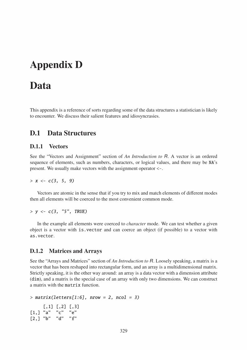
Appendix D
Data
This appendix is a reference of sorts regarding some of the data structures a statistician is likelyto encounter. We discuss their salient features and idiosyncrasies.
D.1 Data Structures
D.1.1 Vectors
See the “Vectors and Assignment” section of An Introduction to R . A vector is an orderedsequence of elements, such as numbers, characters, or logical values, and there may be NA’spresent. We usually make vectors with the assignment operator <-.
> x <- c(3, 5, 9)
Vectors are atomic in the sense that if you try to mix and match elements of di!erent modesthen all elements will be coerced to the most convenient common mode.
> y <- c(3, "5", TRUE)
In the example all elements were coerced to character mode. We can test whether a givenobject is a vector with is.vector and can coerce an object (if possible) to a vector withas.vector.
D.1.2 Matrices and Arrays
See the “Arrays and Matrices” section of An Introduction to R . Loosely speaking, a matrix is avector that has been reshaped into rectangular form, and an array is a multidimensional matrix.Strictly speaking, it is the other way around: an array is a data vector with a dimension attribute(dim), and a matrix is the special case of an array with only two dimensions. We can constructa matrix with the matrix function.
> matrix(letters[1:6], nrow = 2, ncol = 3)
[,1] [,2] [,3]
[1,] "a" "c" "e"
[2,] "b" "d" "f"
329
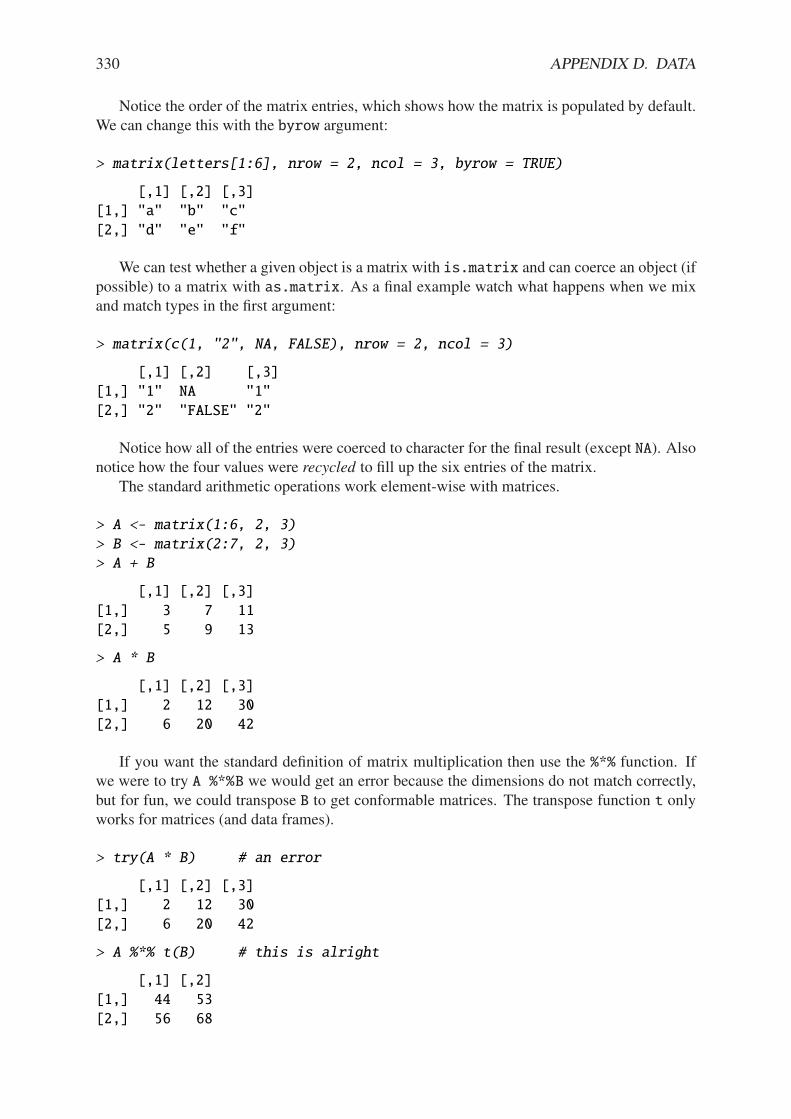
330 APPENDIX D. DATA
Notice the order of the matrix entries, which shows how the matrix is populated by default.We can change this with the byrow argument:
> matrix(letters[1:6], nrow = 2, ncol = 3, byrow = TRUE)
[,1] [,2] [,3]
[1,] "a" "b" "c"
[2,] "d" "e" "f"
We can test whether a given object is a matrix with is.matrix and can coerce an object (ifpossible) to a matrix with as.matrix. As a final example watch what happens when we mixand match types in the first argument:
> matrix(c(1, "2", NA, FALSE), nrow = 2, ncol = 3)
[,1] [,2] [,3]
[1,] "1" NA "1"
[2,] "2" "FALSE" "2"
Notice how all of the entries were coerced to character for the final result (except NA). Alsonotice how the four values were recycled to fill up the six entries of the matrix.
The standard arithmetic operations work element-wise with matrices.
> A <- matrix(1:6, 2, 3)
> B <- matrix(2:7, 2, 3)
> A + B
[,1] [,2] [,3]
[1,] 3 7 11
[2,] 5 9 13
> A * B
[,1] [,2] [,3]
[1,] 2 12 30
[2,] 6 20 42
If you want the standard definition of matrix multiplication then use the %*% function. Ifwe were to try A %*%B we would get an error because the dimensions do not match correctly,but for fun, we could transpose B to get conformable matrices. The transpose function t onlyworks for matrices (and data frames).
> try(A * B) # an error
[,1] [,2] [,3]
[1,] 2 12 30
[2,] 6 20 42
> A %*% t(B) # this is alright
[,1] [,2]
[1,] 44 53
[2,] 56 68
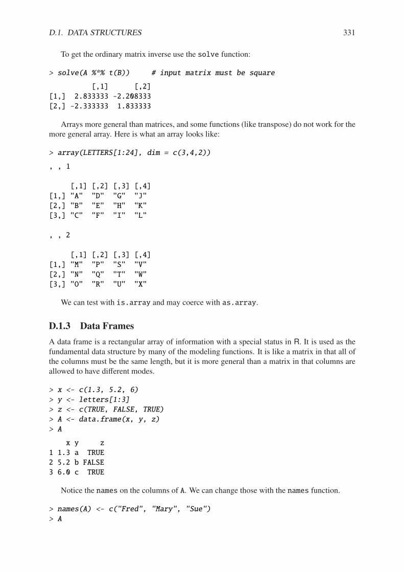
D.1. DATA STRUCTURES 331
To get the ordinary matrix inverse use the solve function:
> solve(A %*% t(B)) # input matrix must be square
[,1] [,2]
[1,] 2.833333 -2.208333
[2,] -2.333333 1.833333
Arrays more general than matrices, and some functions (like transpose) do not work for themore general array. Here is what an array looks like:
> array(LETTERS[1:24], dim = c(3,4,2))
, , 1
[,1] [,2] [,3] [,4]
[1,] "A" "D" "G" "J"
[2,] "B" "E" "H" "K"
[3,] "C" "F" "I" "L"
, , 2
[,1] [,2] [,3] [,4]
[1,] "M" "P" "S" "V"
[2,] "N" "Q" "T" "W"
[3,] "O" "R" "U" "X"
We can test with is.array and may coerce with as.array.
D.1.3 Data Frames
A data frame is a rectangular array of information with a special status in R. It is used as thefundamental data structure by many of the modeling functions. It is like a matrix in that all ofthe columns must be the same length, but it is more general than a matrix in that columns areallowed to have di!erent modes.
> x <- c(1.3, 5.2, 6)
> y <- letters[1:3]
> z <- c(TRUE, FALSE, TRUE)
> A <- data.frame(x, y, z)
> A
x y z
1 1.3 a TRUE
2 5.2 b FALSE
3 6.0 c TRUE
Notice the names on the columns of A. We can change those with the names function.
> names(A) <- c("Fred", "Mary", "Sue")
> A
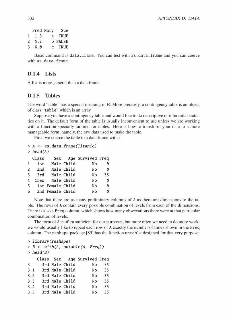
332 APPENDIX D. DATA
Fred Mary Sue
1 1.3 a TRUE
2 5.2 b FALSE
3 6.0 c TRUE
Basic command is data.frame. You can test with is.data.frame and you can coercewith as.data.frame.
D.1.4 Lists
A list is more general than a data frame.
D.1.5 Tables
The word “table” has a special meaning in R. More precisely, a contingency table is an objectof class “table” which is an array
Suppose you have a contingency table and would like to do descriptive or inferential statis-tics on it. The default form of the table is usually inconvenient to use unless we are workingwith a function specially tailored for tables. Here is how to transform your data to a moremanageable form, namely, the raw data used to make the table.
First, we coerce the table to a data frame with :
> A <- as.data.frame(Titanic)
> head(A)
Class Sex Age Survived Freq
1 1st Male Child No 0
2 2nd Male Child No 0
3 3rd Male Child No 35
4 Crew Male Child No 0
5 1st Female Child No 0
6 2nd Female Child No 0
Note that there are as many preliminary columns of A as there are dimensions to the ta-ble. The rows of A contain every possible combination of levels from each of the dimensions.There is also a Freq column, which shows how many observations there were at that particularcombination of levels.
The form of A is often su"cient for our purposes, but more often we need to do more work:we would usually like to repeat each row of A exactly the number of times shown in the Freqcolumn. The reshape package [89] has the function untable designed for that very purpose:
> library(reshape)
> B <- with(A, untable(A, Freq))
> head(B)
Class Sex Age Survived Freq
3 3rd Male Child No 35
3.1 3rd Male Child No 35
3.2 3rd Male Child No 35
3.3 3rd Male Child No 35
3.4 3rd Male Child No 35
3.5 3rd Male Child No 35
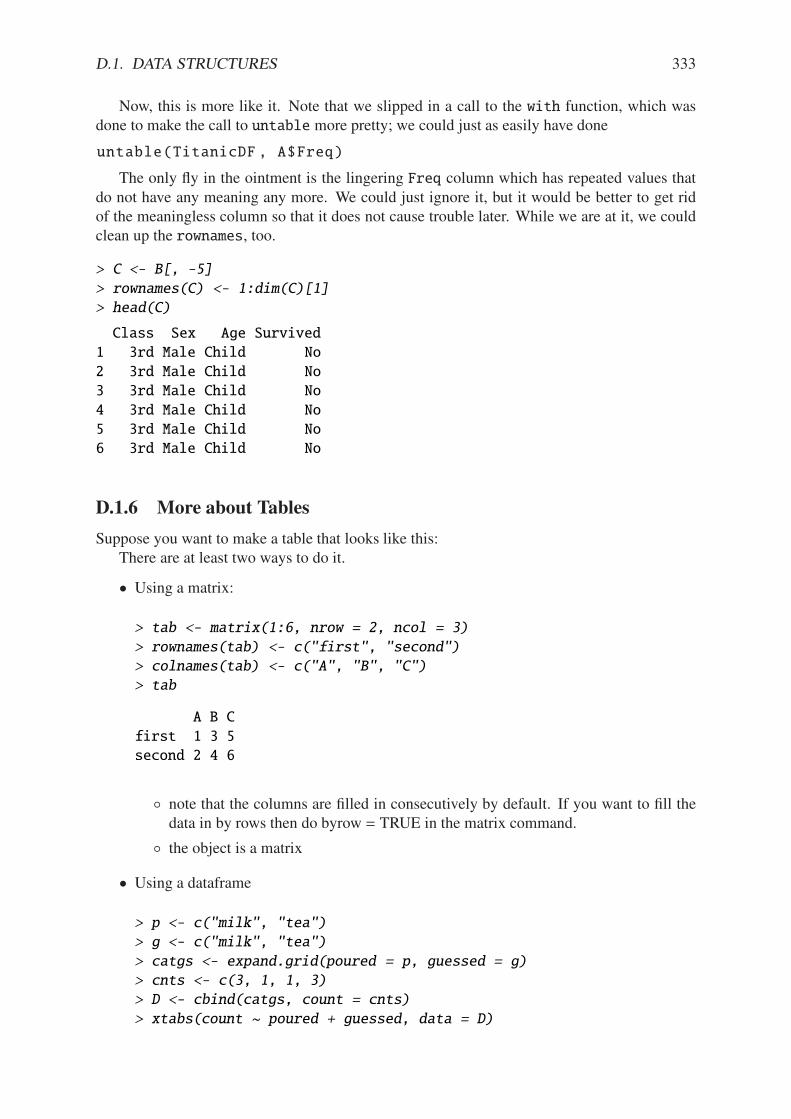
D.1. DATA STRUCTURES 333
Now, this is more like it. Note that we slipped in a call to the with function, which wasdone to make the call to untable more pretty; we could just as easily have done
untable(TitanicDF , A$Freq)
The only fly in the ointment is the lingering Freq column which has repeated values thatdo not have any meaning any more. We could just ignore it, but it would be better to get ridof the meaningless column so that it does not cause trouble later. While we are at it, we couldclean up the rownames, too.
> C <- B[, -5]
> rownames(C) <- 1:dim(C)[1]
> head(C)
Class Sex Age Survived
1 3rd Male Child No
2 3rd Male Child No
3 3rd Male Child No
4 3rd Male Child No
5 3rd Male Child No
6 3rd Male Child No
D.1.6 More about Tables
Suppose you want to make a table that looks like this:There are at least two ways to do it.
• Using a matrix:
> tab <- matrix(1:6, nrow = 2, ncol = 3)
> rownames(tab) <- c("first", "second")
> colnames(tab) <- c("A", "B", "C")
> tab
A B C
first 1 3 5
second 2 4 6
* note that the columns are filled in consecutively by default. If you want to fill thedata in by rows then do byrow = TRUE in the matrix command.
* the object is a matrix
• Using a dataframe
> p <- c("milk", "tea")
> g <- c("milk", "tea")
> catgs <- expand.grid(poured = p, guessed = g)
> cnts <- c(3, 1, 1, 3)
> D <- cbind(catgs, count = cnts)
> xtabs(count ~ poured + guessed, data = D)
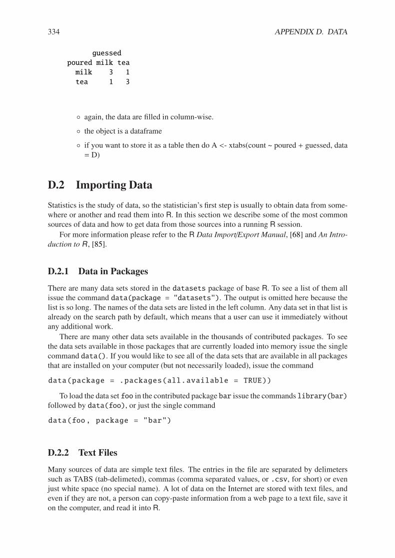
334 APPENDIX D. DATA
guessed
poured milk tea
milk 3 1
tea 1 3
* again, the data are filled in column-wise.
* the object is a dataframe
* if you want to store it as a table then do A <- xtabs(count ~ poured + guessed, data= D)
D.2 Importing Data
Statistics is the study of data, so the statistician’s first step is usually to obtain data from some-where or another and read them into R. In this section we describe some of the most commonsources of data and how to get data from those sources into a running R session.
For more information please refer to the R Data Import/Export Manual, [68] and An Intro-
duction to R , [85].
D.2.1 Data in Packages
There are many data sets stored in the datasets package of base R. To see a list of them allissue the command data(package = "datasets"). The output is omitted here because thelist is so long. The names of the data sets are listed in the left column. Any data set in that list isalready on the search path by default, which means that a user can use it immediately withoutany additional work.
There are many other data sets available in the thousands of contributed packages. To seethe data sets available in those packages that are currently loaded into memory issue the singlecommand data(). If you would like to see all of the data sets that are available in all packagesthat are installed on your computer (but not necessarily loaded), issue the command
data(package = .packages(all.available = TRUE))
To load the data set foo in the contributed package bar issue the commands library(bar)followed by data(foo), or just the single command
data(foo, package = "bar")
D.2.2 Text Files
Many sources of data are simple text files. The entries in the file are separated by delimeterssuch as TABS (tab-delimeted), commas (comma separated values, or .csv, for short) or evenjust white space (no special name). A lot of data on the Internet are stored with text files, andeven if they are not, a person can copy-paste information from a web page to a text file, save iton the computer, and read it into R.
D.3. CREATING NEW DATA SETS 335
D.2.3 Other Software Files
Often the data set of interest is stored in some other, proprietary, format by third-party softwaresuch as Minitab, SAS, or SPSS. The foreign package supports import/conversion from manyof these formats. Please note, however, that data sets from other software sometimes haveproperties with no direct analogue in R. In those cases the conversion process may lose someinformation which will need to be reentered manually from within R. See the Data Import/Ex-
port Manual.
As an example, suppose the data are stored in the SPSS file foo.sav which the user hascopied to the working directory; it can be imported with the commands
> library(foreign)
> read.spss("foo.sav")
See ?read.spss for the available options to customize the file import. Note that the RCommander will import many of the common file types with a menu driven interface.
D.2.4 Importing a Data Frame
The basic command is read.table.
D.3 Creating New Data Sets
Using c
Using scan
Using the R Commander.
D.4 Editing Data
D.4.1 Editing Data Values
D.4.2 Inserting Rows and Columns
D.4.3 Deleting Rows and Columns
D.4.4 Sorting Data
We can sort a vector with the sort function. Normally we have a data frame of several columns(variables) and many, many rows (observations). The goal is to shu#e the rows so that they areordered by the values of one or more columns. This is done with the order function.
For example, we may sort all of the rows of the Puromycin data (in ascending order) bythe variable conc with the following:
> Tmp <- Puromycin[order(Puromycin$conc), ]
> head(Tmp)
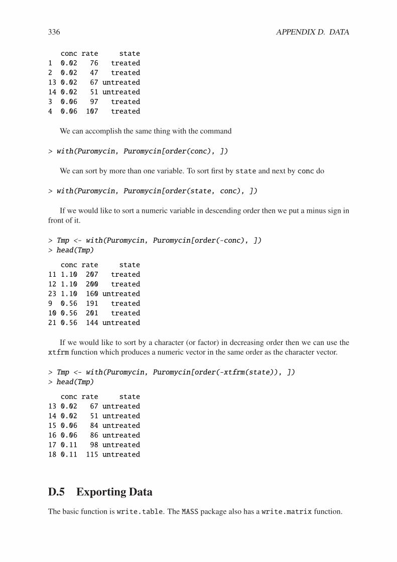
336 APPENDIX D. DATA
conc rate state
1 0.02 76 treated
2 0.02 47 treated
13 0.02 67 untreated
14 0.02 51 untreated
3 0.06 97 treated
4 0.06 107 treated
We can accomplish the same thing with the command
> with(Puromycin, Puromycin[order(conc), ])
We can sort by more than one variable. To sort first by state and next by conc do
> with(Puromycin, Puromycin[order(state, conc), ])
If we would like to sort a numeric variable in descending order then we put a minus sign infront of it.
> Tmp <- with(Puromycin, Puromycin[order(-conc), ])
> head(Tmp)
conc rate state
11 1.10 207 treated
12 1.10 200 treated
23 1.10 160 untreated
9 0.56 191 treated
10 0.56 201 treated
21 0.56 144 untreated
If we would like to sort by a character (or factor) in decreasing order then we can use thextfrm function which produces a numeric vector in the same order as the character vector.
> Tmp <- with(Puromycin, Puromycin[order(-xtfrm(state)), ])
> head(Tmp)
conc rate state
13 0.02 67 untreated
14 0.02 51 untreated
15 0.06 84 untreated
16 0.06 86 untreated
17 0.11 98 untreated
18 0.11 115 untreated
D.5 Exporting Data
The basic function is write.table. The MASS package also has a write.matrix function.

D.6. RESHAPING DATA 337
D.6 Reshaping Data
• Aggregation
• Convert Tables to data frames and back
rbind, cbindab[order(ab[,1]),]
complete.cases
aggregate
stack

338 APPENDIX D. DATA

Appendix E
Mathematical Machinery
This appendix houses many of the standard definitions and theorems that are used at somepoint during the narrative. It is targeted for someone reading the book who forgets the precisedefinition of something and would like a quick reminder of an exact statement. No proofs aregiven, and the interested reader should consult a good text on Calculus (say, Stewart [80] orApostol [4, 5]), Linear Algebra (say, Strang [82] and Magnus [62]), Real Analysis (say, Folland[27], or Carothers [12]), or Measure Theory (Billingsley [8], Ash [6], Resnick [70]) for details.
E.1 Set Algebra
We denote sets by capital letters, A, B, C, etc. The letter S is reserved for the sample space,also known as the universe or universal set, the set which contains all possible elements. Thesymbol , represents the empty set, the set with no elements.
Set Union, Intersection, and Di!erence
Given subsets A and B, we may manipulate them in an algebraic fashion. To this end, wehave three set operations at our disposal: union, intersection, and di!erence. Below is a tablesummarizing the pertinent information about these operations.
Identities and Properties
1. A - , = A, A + , = ,
2. A - S = S , A + S = A
3. A - Ac = S , A + Ac = ,
4. (Ac)c = A
Name Denoted Defined by elements R syntaxUnion A - B in A or B or both union(A, B)
Intersection A + B in both A and B intersect(A, B)
Di!erence A\B in A but not in B setdiff(A, B)
Complement Ac in S but not in A setdiff(S, A)
Table E.1: Set operations
339
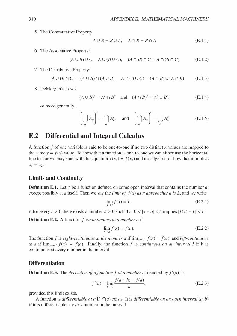
340 APPENDIX E. MATHEMATICAL MACHINERY
5. The Commutative Property:
A - B = B - A, A + B = B + A (E.1.1)
6. The Associative Property:
(A - B) - C = A - (B -C), (A + B) + C = A + (B +C) (E.1.2)
7. The Distributive Property:
A - (B +C) = (A - B) + (A - B), A + (B -C) = (A + B) - (A + B) (E.1.3)
8. DeMorgan’s Laws
(A - B)c = Ac + Bc and (A + B)c = Ac - Bc, (E.1.4)
or more generally,$%%%%%&'
(
A(
()))))*
c
=+
(
Ac(, and
$%%%%%&+
(
A(
()))))*
c
='
(
Ac( (E.1.5)
E.2 Di!erential and Integral Calculus
A function f of one variable is said to be one-to-one if no two distinct x values are mapped tothe same y = f (x) value. To show that a function is one-to-one we can either use the horizontalline test or we may start with the equation f (x1) = f (x2) and use algebra to show that it impliesx1 = x2.
Limits and Continuity
Definition E.1. Let f be a function defined on some open interval that contains the number a,except possibly at a itself. Then we say the limit of f (x) as x approaches a is L, and we write
limx.a
f (x) = L, (E.2.1)
if for every $ > 0 there exists a number . > 0 such that 0 < |x # a| < . implies | f (x) # L| < $.
Definition E.2. A function f is continuous at a number a if
limx.a
f (x) = f (a). (E.2.2)
The function f is right-continuous at the number a if limx.a+ f (x) = f (a), and left-continuous
at a if limx.a# f (x) = f (a). Finally, the function f is continuous on an interval I if it iscontinuous at every number in the interval.
Di!erentiation
Definition E.3. The derivative of a function f at a number a, denoted by f 5(a), is
f 5(a) = limh.0
f (a + h) # f (a)
h, (E.2.3)
provided this limit exists.A function is di"erentiable at a if f 5(a) exists. It is di"erentiable on an open interval (a, b)
if it is di!erentiable at every number in the interval.
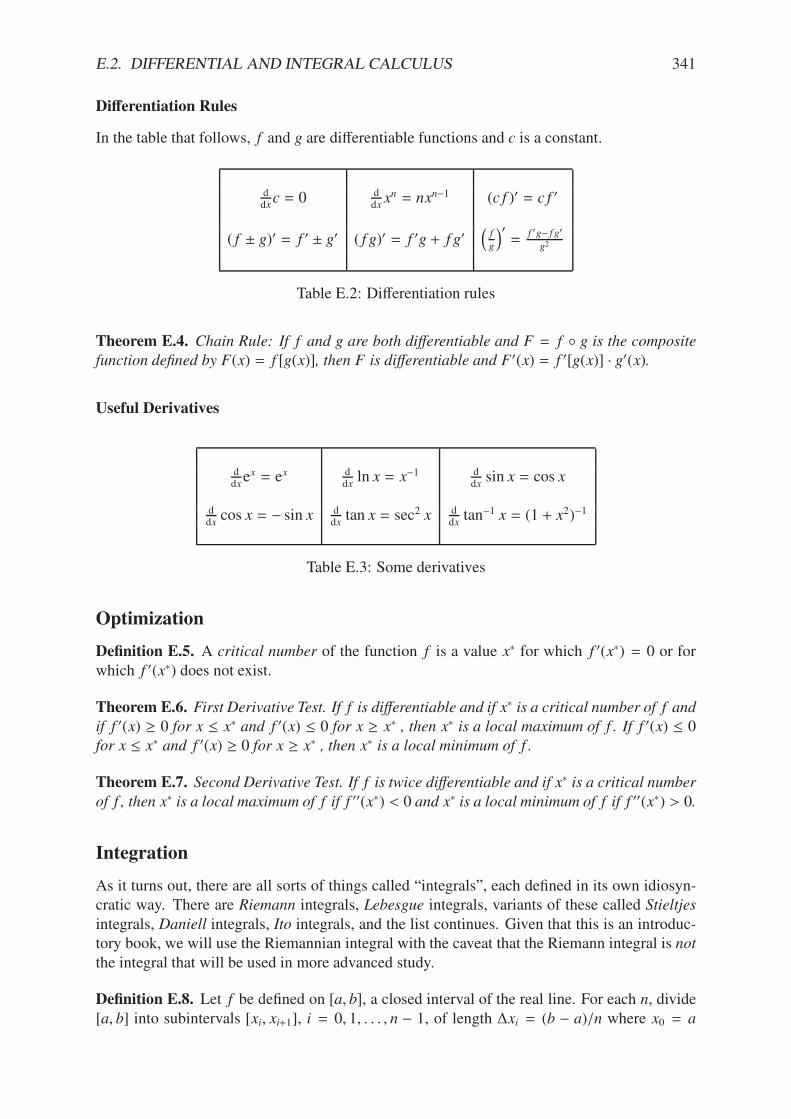
E.2. DIFFERENTIAL AND INTEGRAL CALCULUS 341
Di!erentiation Rules
In the table that follows, f and g are di!erentiable functions and c is a constant.
ddxc = 0 d
dxxn = nxn#1 (c f )5 = c f 5
( f ± g)5 = f 5 ± g5 ( f g)5 = f 5g + f g52f
g
35=
f 5g# f g5
g2
Table E.2: Di!erentiation rules
Theorem E.4. Chain Rule: If f and g are both di"erentiable and F = f * g is the composite
function defined by F(x) = f [g(x)], then F is di"erentiable and F5(x) = f 5[g(x)] · g5(x).
Useful Derivatives
ddxex = ex d
dxln x = x#1 d
dxsin x = cos x
ddxcos x = # sin x d
dxtan x = sec2 x d
dxtan#1 x = (1 + x2)#1
Table E.3: Some derivatives
Optimization
Definition E.5. A critical number of the function f is a value x6 for which f 5(x6) = 0 or forwhich f 5(x6) does not exist.
Theorem E.6. First Derivative Test. If f is di"erentiable and if x6 is a critical number of f andif f 5(x) / 0 for x " x6 and f 5(x) " 0 for x / x6 , then x6 is a local maximum of f . If f 5(x) " 0for x " x6 and f 5(x) / 0 for x / x6 , then x6 is a local minimum of f .
Theorem E.7. Second Derivative Test. If f is twice di"erentiable and if x6 is a critical number
of f , then x6 is a local maximum of f if f 55(x6) < 0 and x6 is a local minimum of f if f 55(x6) > 0.
Integration
As it turns out, there are all sorts of things called “integrals”, each defined in its own idiosyn-cratic way. There are Riemann integrals, Lebesgue integrals, variants of these called Stieltjes
integrals, Daniell integrals, Ito integrals, and the list continues. Given that this is an introduc-tory book, we will use the Riemannian integral with the caveat that the Riemann integral is notthe integral that will be used in more advanced study.
Definition E.8. Let f be defined on [a, b], a closed interval of the real line. For each n, divide[a, b] into subintervals [xi, xi+1], i = 0, 1, . . . , n # 1, of length (xi = (b # a)/n where x0 = a
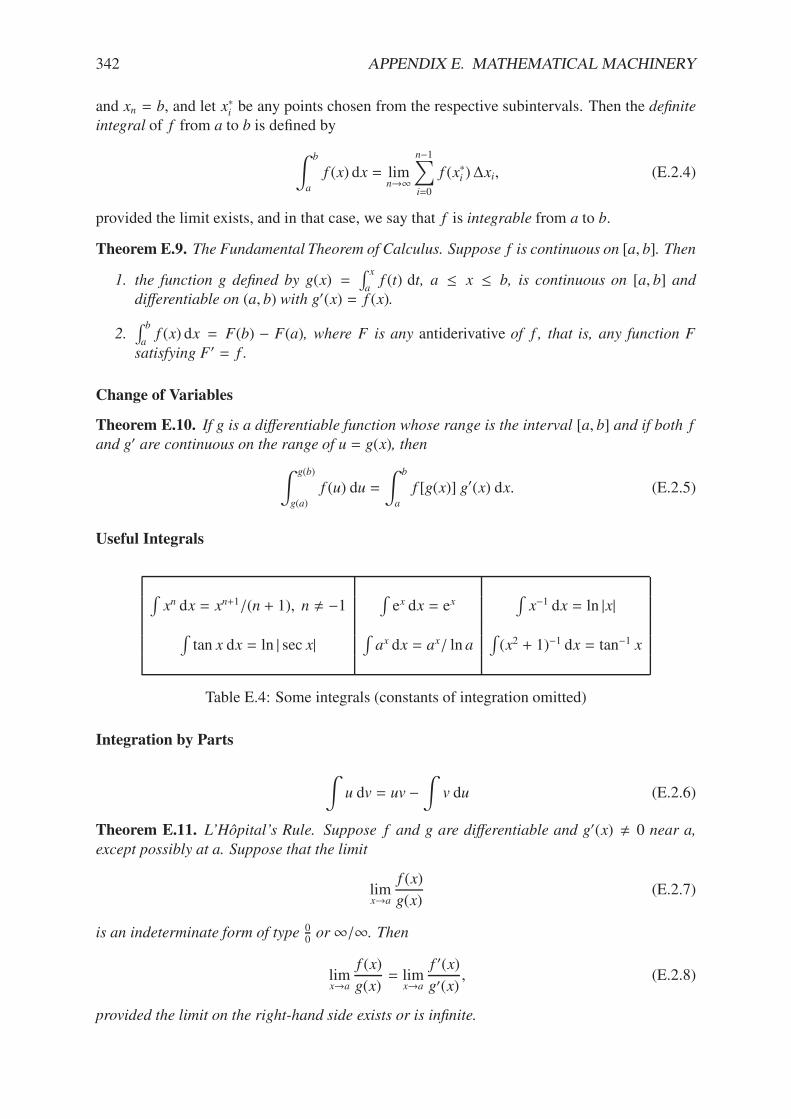
342 APPENDIX E. MATHEMATICAL MACHINERY
and xn = b, and let x6i be any points chosen from the respective subintervals. Then the definiteintegral of f from a to b is defined by
B b
a
f (x) dx = limn.&
n#1!
i=0
f (x6i )(xi, (E.2.4)
provided the limit exists, and in that case, we say that f is integrable from a to b.
Theorem E.9. The Fundamental Theorem of Calculus. Suppose f is continuous on [a, b]. Then
1. the function g defined by g(x) =A x
af (t) dt, a " x " b, is continuous on [a, b] and
di"erentiable on (a, b) with g5(x) = f (x).
2.A b
af (x) dx = F(b) # F(a), where F is any antiderivative of f , that is, any function F
satisfying F5 = f .
Change of Variables
Theorem E.10. If g is a di"erentiable function whose range is the interval [a, b] and if both f
and g5 are continuous on the range of u = g(x), then
B g(b)
g(a)
f (u) du =
B b
a
f [g(x)] g5(x) dx. (E.2.5)
Useful Integrals
Axn dx = xn+1/(n + 1), n ! #1
Aex dx = ex
Ax#1 dx = ln |x|
Atan x dx = ln | sec x|
Aax dx = ax/ ln a
A(x2 + 1)#1 dx = tan#1 x
Table E.4: Some integrals (constants of integration omitted)
Integration by Parts
Bu dv = uv #
Bv du (E.2.6)
Theorem E.11. L’Hôpital’s Rule. Suppose f and g are di"erentiable and g5(x) ! 0 near a,
except possibly at a. Suppose that the limit
limx.a
f (x)
g(x)(E.2.7)
is an indeterminate form of type 00or&/&. Then
limx.a
f (x)
g(x)= lim
x.a
f 5(x)
g5(x), (E.2.8)
provided the limit on the right-hand side exists or is infinite.
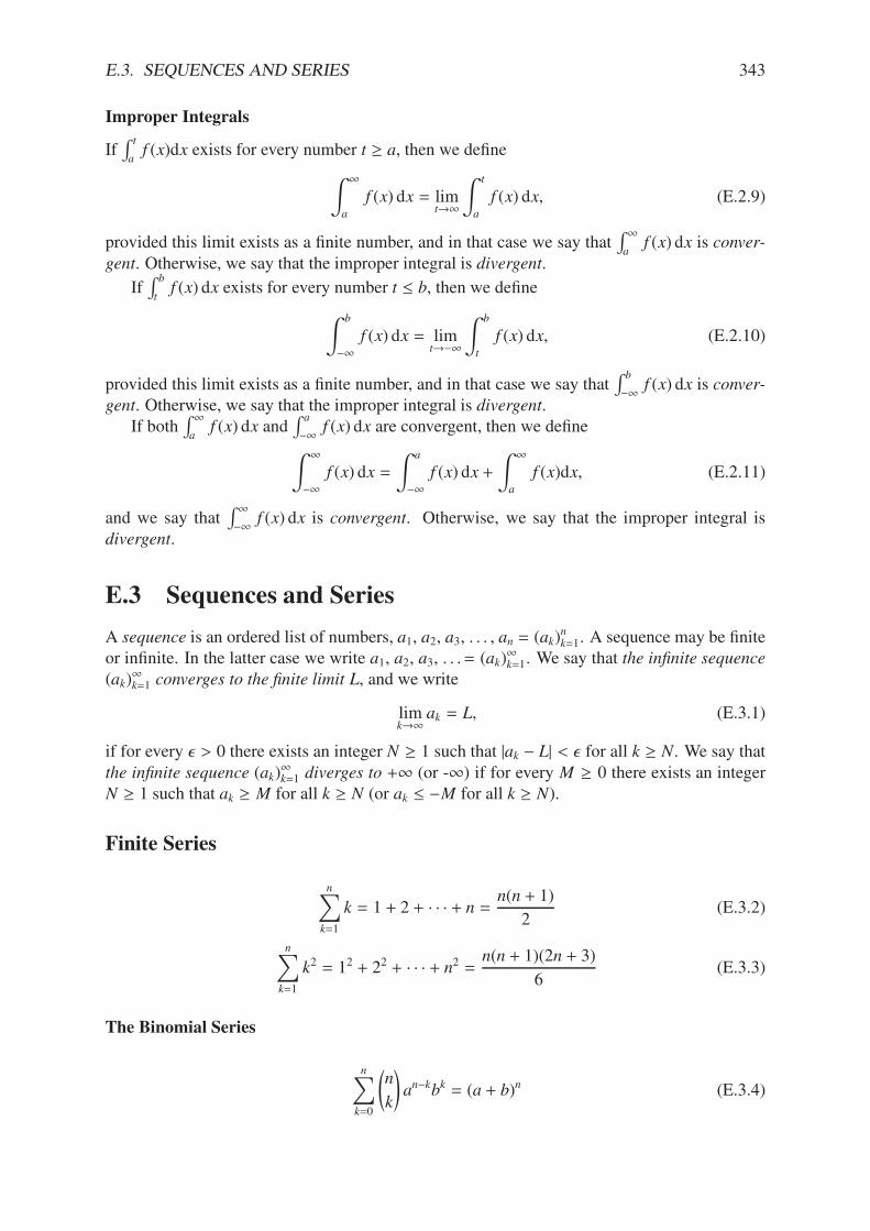
E.3. SEQUENCES AND SERIES 343
Improper Integrals
IfA t
af (x)dx exists for every number t / a, then we define
B &
a
f (x) dx = limt.&
B t
a
f (x) dx, (E.2.9)
provided this limit exists as a finite number, and in that case we say thatA &
af (x) dx is conver-
gent. Otherwise, we say that the improper integral is divergent.
IfA b
tf (x) dx exists for every number t " b, then we define
B b
#&f (x) dx = lim
t.#&
B b
t
f (x) dx, (E.2.10)
provided this limit exists as a finite number, and in that case we say thatA b
#& f (x) dx is conver-gent. Otherwise, we say that the improper integral is divergent.
If bothA &
af (x) dx and
A a
#&f (x) dx are convergent, then we define
B &
#&f (x) dx =
B a
#&f (x) dx +
B &
a
f (x)dx, (E.2.11)
and we say thatA &
#& f (x) dx is convergent. Otherwise, we say that the improper integral isdivergent.
E.3 Sequences and Series
A sequence is an ordered list of numbers, a1, a2, a3, . . . , an = (ak)nk=1. A sequence may be finite
or infinite. In the latter case we write a1, a2, a3, . . .= (ak)&k=1. We say that the infinite sequence
(ak)&k=1 converges to the finite limit L, and we write
limk.&
ak = L, (E.3.1)
if for every $ > 0 there exists an integer N / 1 such that |ak # L| < $ for all k / N. We say thatthe infinite sequence (ak)
&k=1 diverges to +& (or -&) if for every M / 0 there exists an integer
N / 1 such that ak / M for all k / N (or ak " #M for all k / N).
Finite Series
n!
k=1
k = 1 + 2 + · · · + n =n(n + 1)
2(E.3.2)
n!
k=1
k2 = 12 + 22 + · · · + n2 =n(n + 1)(2n + 3)
6(E.3.3)
The Binomial Series
n!
k=0
0n
k
1an#kbk = (a + b)n (E.3.4)
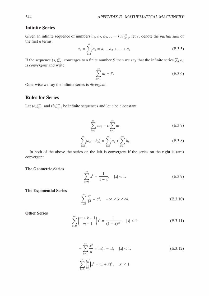
344 APPENDIX E. MATHEMATICAL MACHINERY
Infinite Series
Given an infinite sequence of numbers a1, a2, a3, . . .= (ak)&k=1, let sn denote the partial sum of
the first n terms:
sn =
n!
k=1
ak = a1 + a2 + · · · + an. (E.3.5)
If the sequence (sn)&n=1 converges to a finite number S then we say that the infinite series
#k ak
is convergent and write&!
k=1
ak = S . (E.3.6)
Otherwise we say the infinite series is divergent.
Rules for Series
Let (ak)&k=1 and (bk)
&k=1 be infinite sequences and let c be a constant.
&!
k=1
cak = c
&!
k=1
ak (E.3.7)
&!
k=1
(ak ± bk) =&!
k=1
ak ±&!
k=1
bk (E.3.8)
In both of the above the series on the left is convergent if the series on the right is (are)convergent.
The Geometric Series&!
k=0
xk =1
1 # x, |x| < 1. (E.3.9)
The Exponential Series&!
k=0
xk
k!= ex, #& < x < &. (E.3.10)
Other Series&!
k=0
0m + k # 1
m # 1
1xk =
1
(1 # x)m, |x| < 1. (E.3.11)
#&!
k=1
xn
n= ln(1 # x), |x| < 1. (E.3.12)
&!
k=0
0n
k
1xk = (1 + x)n, |x| < 1.
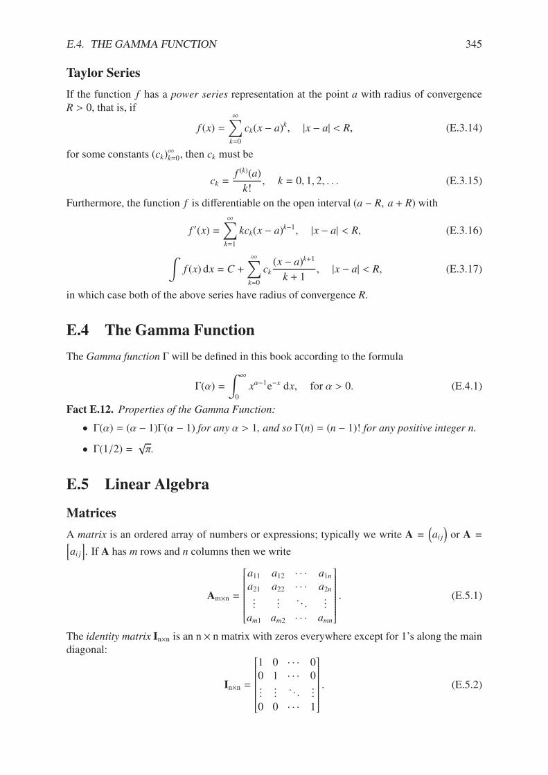
E.4. THE GAMMA FUNCTION 345
Taylor Series
If the function f has a power series representation at the point a with radius of convergenceR > 0, that is, if
f (x) =&!
k=0
ck(x # a)k, |x # a| < R, (E.3.14)
for some constants (ck)&k=0, then ck must be
ck =f (k)(a)
k!, k = 0, 1, 2, . . . (E.3.15)
Furthermore, the function f is di!erentiable on the open interval (a # R, a + R) with
f 5(x) =&!
k=1
kck(x # a)k#1, |x # a| < R, (E.3.16)
Bf (x) dx = C +
&!
k=0
ck(x # a)k+1
k + 1, |x # a| < R, (E.3.17)
in which case both of the above series have radius of convergence R.
E.4 The Gamma Function
The Gamma function % will be defined in this book according to the formula
%(() =
B &
0
x(#1e#x dx, for ( > 0. (E.4.1)
Fact E.12. Properties of the Gamma Function:
• %(() = (( # 1)%(( # 1) for any ( > 1, and so %(n) = (n # 1)! for any positive integer n.
• %(1/2) =$&.
E.5 Linear Algebra
Matrices
A matrix is an ordered array of numbers or expressions; typically we write A =2ai j
3or A =C
ai jD. If A has m rows and n columns then we write
Am7n =
EFFFFFFFFFFFFFFFG
a11 a12 · · · a1na21 a22 · · · a2n...
.... . .
...
am1 am2 · · · amn
HIIIIIIIIIIIIIIIJ. (E.5.1)
The identity matrix In7n is an n 7 n matrix with zeros everywhere except for 1’s along the maindiagonal:
In7n =
EFFFFFFFFFFFFFFFG
1 0 · · · 00 1 · · · 0....... . .
...
0 0 · · · 1
HIIIIIIIIIIIIIIIJ. (E.5.2)
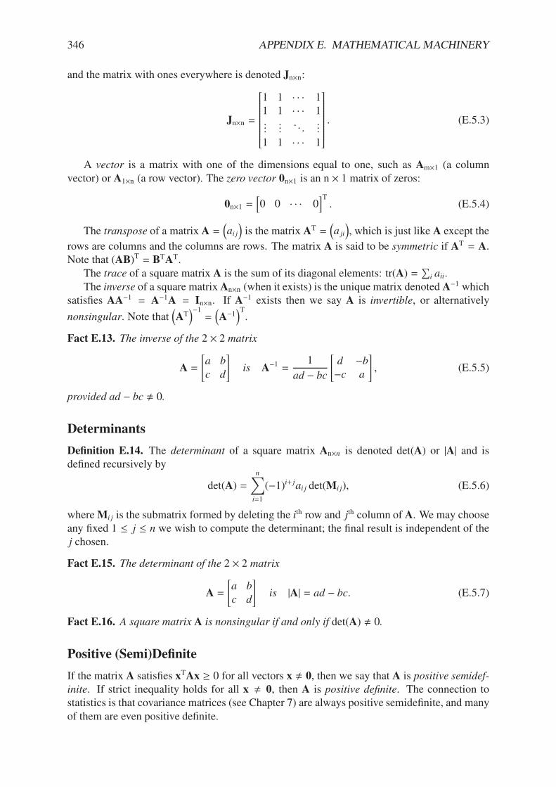
346 APPENDIX E. MATHEMATICAL MACHINERY
and the matrix with ones everywhere is denoted Jn7n:
Jn7n =
EFFFFFFFFFFFFFFFG
1 1 · · · 11 1 · · · 1....... . .
...
1 1 · · · 1
HIIIIIIIIIIIIIIIJ. (E.5.3)
A vector is a matrix with one of the dimensions equal to one, such as Am71 (a columnvector) or A17n (a row vector). The zero vector 0n71 is an n 7 1 matrix of zeros:
0n71 =C0 0 · · · 0
DT. (E.5.4)
The transpose of a matrix A =2ai j
3is the matrix AT =
2aji
3, which is just like A except the
rows are columns and the columns are rows. The matrix A is said to be symmetric if AT = A.Note that (AB)T = BTAT.
The trace of a square matrix A is the sum of its diagonal elements: tr(A) =#
i aii.The inverse of a square matrixAn7n (when it exists) is the unique matrix denoted A#1 which
satisfies AA#1 = A#1A = In7n. If A#1 exists then we say A is invertible, or alternatively
nonsingular. Note that2AT
3#1=
2A#1
3T.
Fact E.13. The inverse of the 2 7 2 matrix
A =
7a b
c d
8is A#1 =
1
ad # bc
7d #b#c a
8, (E.5.5)
provided ad # bc ! 0.
Determinants
Definition E.14. The determinant of a square matrix An7n is denoted det(A) or |A| and isdefined recursively by
det(A) =n!
i=1
(#1)i+ jai j det(Mi j), (E.5.6)
whereMi j is the submatrix formed by deleting the ith row and jth column of A. We may chooseany fixed 1 " j " n we wish to compute the determinant; the final result is independent of thej chosen.
Fact E.15. The determinant of the 2 7 2 matrix
A =
7a b
c d
8is |A| = ad # bc. (E.5.7)
Fact E.16. A square matrix A is nonsingular if and only if det(A) ! 0.
Positive (Semi)Definite
If the matrix A satisfies xTAx / 0 for all vectors x ! 0, then we say that A is positive semidef-inite. If strict inequality holds for all x ! 0, then A is positive definite. The connection tostatistics is that covariance matrices (see Chapter 7) are always positive semidefinite, and manyof them are even positive definite.

E.6. MULTIVARIABLE CALCULUS 347
E.6 Multivariable Calculus
Partial Derivatives
If f is a function of two variables, its first-order partial derivatives are defined by
- f
-x=-
-xf (x, y) = lim
h.0
f (x + h, y) # f (x, y)
h(E.6.1)
and- f
-y=-
-yf (x, y) = lim
h.0
f (x, y + h) # f (x, y)
h, (E.6.2)
provided these limits exist. The second-order partial derivatives of f are defined by
-2 f
-x2=-
-x
0- f
-x
1,-2 f
-y2=-
-y
0- f
-y
1,-2 f
-x-y=-
-x
0- f
-y
1,-2 f
-y-x=-
-y
0- f
-x
1. (E.6.3)
In many cases (and for all cases in this book) it is true that
-2 f
-x-y=-2 f
-y-x. (E.6.4)
Optimization
An function f of two variables has a local maximum at (a, b) if f (x, y) / f (a, b) for all points(x, y) near (a, b), that is, for all points in an open disk centered at (a, b). The number f (a, b) isthen called a local maximum value of f . The function f has a local minimum if the same thinghappens with the inequality reversed.
Suppose the point (a, b) is a critical point of f , that is, suppose (a, b) satisfies
- f
-x(a, b) =
- f
-y(a, b) = 0. (E.6.5)
Further suppose -2 f
-x2and -
2 f
-y2are continuous near (a, b). Let the Hessian matrix H (not to be
confused with the hat matrix H of Chapter 12) be defined by
H =
EFFFFFFG-2 f
-x2-2 f
-x-y-2 f
-y-x
-2 f
-y2
HIIIIIIJ . (E.6.6)
We use the following rules to decide whether (a, b) is an extremum (that is, a local minimum orlocal maximum) of f .
• If det(H) > 0 and -2 f
-x2(a, b) > 0, then (a, b) is a local minimum of f .
• If det(H) > 0 and -2 f
-x2(a, b) < 0, then (a, b) is a local maximum of f .
• If det(H) < 0, then (a, b) is a saddle point of f and so is not an extremum of f .
• If det(H) = 0, then we do not know the status of (a, b); it might be an extremum or itmight not be.
348 APPENDIX E. MATHEMATICAL MACHINERY
Double and Multiple Integrals
Let f be defined on a rectangle R = [a, b]7[c, d], and for eachm and n divide [a, b] (respectively[c, d]) into subintervals [x j, x j+1], i = 0, 1, . . . ,m # 1 (respectively [yi, yi+1]) of length (x j =
(b # a)/m (respectively (yi = (d # c)/n) where x0 = a and xm = b (and y0 = c and yn = d ), andlet x6j (y
6i ) be any points chosen from their respective subintervals. Then the double integral of
f over the rectangle R is
"R
f (x, y) dA =
dB
c
bB
a
f (x, y) dxdy = limm,n.&
n!
i=1
m!
j=1
f (x6j, y6i )(x j(yi, (E.6.7)
provided this limit exists. Multiple integrals are defined in the same way just with more lettersand sums.
Bivariate and Multivariate Change of Variables
Suppose we have a transformation1 T that maps points (u, v) in a set A to points (x, y) in a set B.We typically write x = x(u, v) and y = y(u, v), and we assume that x and y have continuous first-order partial derivatives. We say that T is one-to-one if no two distinct (u, v) pairs get mappedto the same (x, y) pair; in this book, all of our multivariate transformations T are one-to-one.
The Jacobian (pronounced “yah-KOH-bee-uhn”) of T is denoted by -(x, y)/-(u, v) and isdefined by the determinant of the following matrix of partial derivatives:
-(x, y)
-(u, v)=
444444
-x-u
-x-v
-y
-u
-y
-v
444444 =-x
-u
-y
-v#-x
-v
-y
-u. (E.6.8)
If the function f is continuous on A and if the Jacobian of T is nonzero except perhaps on theboundary of A, then
"B
f (x, y) dx dy =
"A
fRx(u, v), y(u, v)
S 44444-(x, y)
-(u, v)
44444 du dv. (E.6.9)
A multivariate change of variables is defined in an analogous way: the one-to-one transfor-mation T maps points (u1, u2, . . . , un) to points (x1, x2, . . . , xn), the Jacobian is the determinantof the n 7 n matrix of first-order partial derivatives of T (lined up in the natural manner), andinstead of a double integral we have a multiple integral over multidimensional sets A and B.
1For our purposes T is in fact the inverse of a one-to-one transformation that we are initially given. We usuallystart with functions that map (x, y) 9#. (u, v), and one of our first tasks is to solve for the inverse transformationthat maps (u, v) 9#. (x, y). It is this inverse transformation which we are calling T .
Appendix F
Writing Reports with R
Perhaps the most important part of a statistician’s job once the analysis is complete is to com-municate the results to others. This is usually done with some type of report that is delivered tothe client, manager, or administrator. Other situations that call for reports include term papers,final projects, thesis work, etc. This chapter is designed to pass along some tips about writingreports once the work is completed with R.
F.1 What to Write
It is possible to summarize this entire appendix with only one sentence: the statistician’s goalis to communicate with others. To this end, there are some general guidelines that I give tostudents which are based on an outline originally written and shared with me by Dr. G. AndyChang.
Basic Outline for a Statistical Report
1. Executive Summary (a one page description of the study and conclusion)
2. Introduction
(a) What is the question, and why is it important?
(b) Is the study observational or experimental?
(c) What are the hypotheses of interest to the researcher?
(d) What are the types of analyses employed? (one sample t-test, paired-sample t-test,ANOVA, chi-square test, regression, . . . )
3. Data Collection
(a) Describe how the data were collected in detail.
(b) Identify all variable types: quantitative, qualitative, ordered or nominal (with lev-els), discrete, continuous.
(c) Discuss any limitations of the data collection procedure. Look carefully for anysources of bias.
4. Summary Information
349
350 APPENDIX F. WRITING REPORTS WITH R
(a) Give numeric summaries of all variables of interest.
i. Discrete: (relative) frequencies, contingency tables, odds ratios, etc.
ii. Continuous: measures of center, spread, shape.
(b) Give visual summaries of all variables of interest.
i. Side-by-side boxplots, scatterplots, histograms, etc.
(c) Discuss any unusual features of the data (outliers, clusters, granularity, etc.)
(d) Report any missing data and identify any potential problems or bias.
5. Analysis
(a) State any hypotheses employed, and check the assumptions.
(b) Report test statistics, p-values, and confidence intervals.
(c) Interpret the results in the context of the study.
(d) Attach (labeled) tables and/or graphs and make reference to them in the report asneeded.
6. Conclusion
(a) Summarize the results of the study. What did you learn?
(b) Discuss any limitations of the study or inferences.
(c) Discuss avenues of future research suggested by the study.
F.2 How to Write It with R
Once the decision has been made what to write, the next task is to typeset the information to beshared. To do this the author will need to select software to use to write the documents. Thereare many options available, and choosing one over another is sometimes a matter of taste. Butnot all software were created equal, and R plays better with some applications than it does withothers.
In short, R does great with LATEX and there are many resources available to make writing adocument with R and LATEX easier. But LATEX is not for the beginner, and there are other wordprocessors which may be acceptable depending on the circumstances.
F.2.1 Microsoft!Word
It is a fact of life that Microsoft!Windows is currently the most prevalent desktop operatingsystem on the planet. Those who own Windows also typically own some version of MicrosoftO"ce, thus Microsoft Word is the default word processor for many, many people.
The standard way to write an R report with Microsoft!Word is to generate material withR and then copy-paste the material at selected places in a Word document. An advantage tothis approach is that Word is nicely designed to make it easy to copy-and-paste from RGui tothe Word document.
A disadvantage to this approach is that the R input/output needs to be edited manually bythe author to make it readable for others. Another disadvantage is that the approach does not

F.2. HOW TO WRITE IT WITH R 351
work on all operating systems (not on Linux, in particular). Yet another disadvantage is thatMicrosoft! Word is proprietary, and as a result, R does not communicate with Microsoft!Word as well as it does with other software as we shall soon see.
Nevertheless, if you are going to write a report with Word there are some steps that you cantake to make the report more amenable to the reader.
1. Copy and paste graphs into the document. You can do this by right clicking on the graphand selecting Copy as bitmap, or Copy as metafile, or one of the other options. Thenmove the cursor to the document where you want the picture, right-click, and selectPaste.
2. Resize (most) pictures so that they take up no more than 1/2 page. You may want to putgraphs side by side; do this by inserting a table and placing the graphs inside the cells.
3. Copy selected R input and output to the Word document. All code should be separatedfrom the rest of the writing, except when specifically mentioning a function or object ina sentence.
4. The font of R input/output should be Courier New, or some other monowidth font (notTimes New Roman or Calibri); the default font size of 12 is usually too big for R codeand should be reduced to, for example, 10pt.
It is also possible to communicate with R through OpenO"ce.org, which can export to theproprietary (.doc) format.
F.2.2 OpenO"ce.org and odfWeave
OpenO"ce.org (OO.o) is an open source desktop productivity suite which mirrors Microsoft!O"ce. It is especially nice because it works on all operating systems. OO.o can read mostdocument formats, and in particular, it will read .doc files. The standard OO.o file extensionfor documents is .odt, which stands for “open document text”.
The odfWeave package [55] provides a way to generate an .odt file withR input and outputcode formatted correctly and inserted in the correct places, without any additional work. In thisway, one does not need to worry about all of the trouble of typesetting R output. Anotheradvantage of odfWeave is that it allows you to generate the report dynamically; if the dataunderlying the report change or are updated, then a few clicks (or commands) will generate abrand new report.
One disadvantage is that the source .odt file is not easy to read, because it is di"cult tovisually distinguish the noweb parts (where the R code is) from the non-noweb parts. This canbe fixed by manually changing the font of the noweb sections to, for instance, Courier font,size 10pt. But it is extra work. It would be nice if a program would discriminate between thetwo di!erent sections and automatically typeset the respective parts in their correct fonts. Thisis one of the advantages to LYX.
Another advantage of OO.o is that even after you have generated the outfile, it is fullyeditable just like any other .odt document. If there are errors or formatting problems, they canbe fixed at any time.
Here are the basic steps to typeset a statistical report with OO.o.
1. Write your report as an .odt document in OO.o just as you would any other document.Call this document infile.odt, and make sure that it is saved in your working directory.
352 APPENDIX F. WRITING REPORTS WITH R
2. At the places you would like to insert R code in the document, write the code chunks inthe following format:
<<>>=
x <- rnorm(10)
mean(x)
@
or write whatever code you want between the symbols <<>>= and @.
3. Open R and type the following:
> library(odfWeave)
> odfWeave(file = "infile.odt", dest = "outfile.odt")
4. The compiled (.odt) file, complete with all of the R output automatically inserted in thecorrect places, will now be the file outfile.odt located in the working directory. Openoutfile.odt, examine it, modify it, and repeat if desired.
There are all sorts of extra things that can be done. For example, the R commands can be sup-pressed with the tag <<echo = FALSE>>=, and the R output may be hidden with <<results= hide>>=. See the odfWeave package documentation for details.
F.2.3 Sweave and LATEX
This approach is nice because it works for all operating systems. One can quite literally typesetanything with LATEX. All of this power comes at a price, however. The writer must learn theLATEX language which is a nontrivial enterprise. Even given the language, if there is a singlesyntax error, or a single delimeter missing in the entire document, then the whole thing breaks.
LATEX can do anything, but it is relatively di"cult to learn and very grumpy about syntaxerrors and delimiter matching. there are however programs useful for formatting LATEX.
A disadvantage is that you cannot see the mathematical formulas until you run the wholefile with LATEX.
A disadvantage is that figures and tables are relatively di"cult.There are programs to make the process easier AUCTEX
dev.copy2eps, also dev.copy2pdfhttp://www.stat.uni-muenchen.de/~leisch/Sweave/
F.2.4 Sweave and LYX
This approach is nice because it works for all operating systems. It gives you everything fromthe last section and makes it easier to use LATEX. That being said, it is better to know LATEXalready when migrating to LYX, because you understand all of the machinery going on underthe hood.
Program Listings and the R languageThis book was written with LYX.
http://gregor.gorjanc.googlepages.com/lyx-sweave
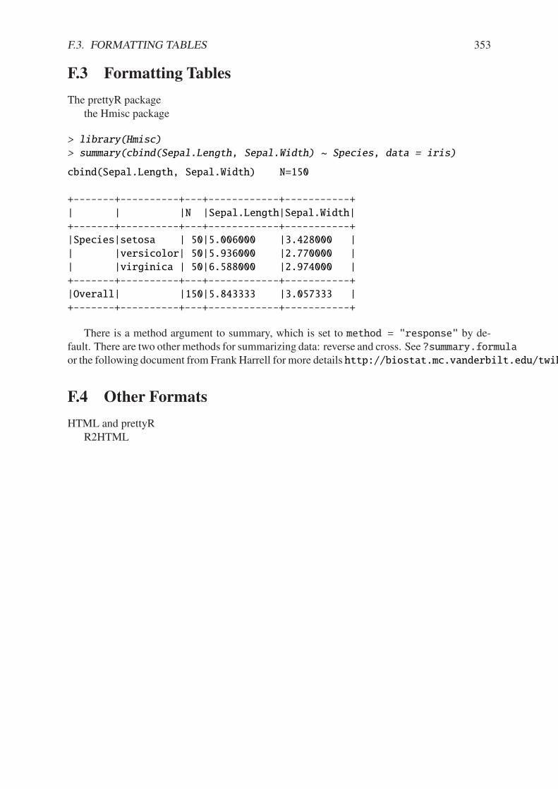
F.3. FORMATTING TABLES 353
F.3 Formatting Tables
The prettyR packagethe Hmisc package
> library(Hmisc)
> summary(cbind(Sepal.Length, Sepal.Width) ~ Species, data = iris)
cbind(Sepal.Length, Sepal.Width) N=150
+-------+----------+---+------------+-----------+
| | |N |Sepal.Length|Sepal.Width|
+-------+----------+---+------------+-----------+
|Species|setosa | 50|5.006000 |3.428000 |
| |versicolor| 50|5.936000 |2.770000 |
| |virginica | 50|6.588000 |2.974000 |
+-------+----------+---+------------+-----------+
|Overall| |150|5.843333 |3.057333 |
+-------+----------+---+------------+-----------+
There is a method argument to summary, which is set to method = "response" by de-fault. There are two other methods for summarizing data: reverse and cross. See ?summary.formulaor the following document from Frank Harrell for more details http://biostat.mc.vanderbilt.edu/twiki
F.4 Other Formats
HTML and prettyRR2HTML

354 APPENDIX F. WRITING REPORTS WITH R
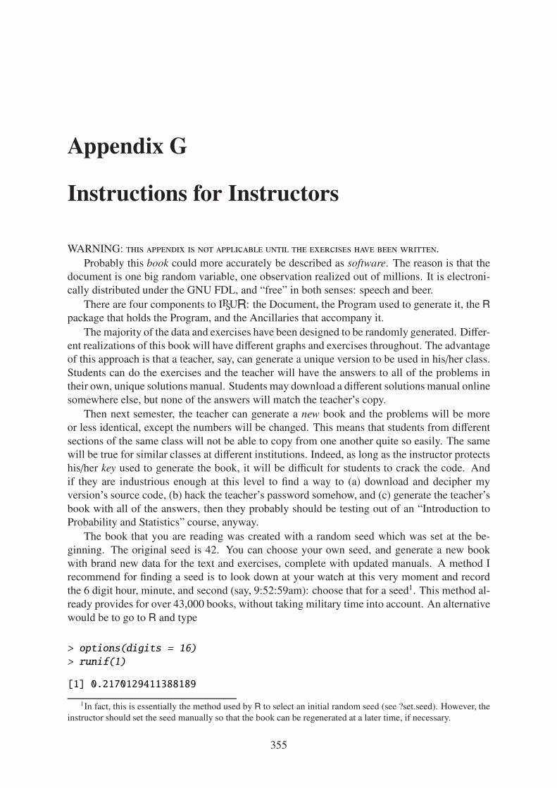
Appendix G
Instructions for Instructors
WARNING: this appendix is not applicable until the exercises have been written.
Probably this book could more accurately be described as software. The reason is that thedocument is one big random variable, one observation realized out of millions. It is electroni-cally distributed under the GNU FDL, and “free” in both senses: speech and beer.
There are four components to IPSUR: the Document, the Program used to generate it, the Rpackage that holds the Program, and the Ancillaries that accompany it.
The majority of the data and exercises have been designed to be randomly generated. Di!er-ent realizations of this book will have di!erent graphs and exercises throughout. The advantageof this approach is that a teacher, say, can generate a unique version to be used in his/her class.Students can do the exercises and the teacher will have the answers to all of the problems intheir own, unique solutionsmanual. Students may download a di!erent solutions manual onlinesomewhere else, but none of the answers will match the teacher’s copy.
Then next semester, the teacher can generate a new book and the problems will be moreor less identical, except the numbers will be changed. This means that students from di!erentsections of the same class will not be able to copy from one another quite so easily. The samewill be true for similar classes at di!erent institutions. Indeed, as long as the instructor protectshis/her key used to generate the book, it will be di"cult for students to crack the code. Andif they are industrious enough at this level to find a way to (a) download and decipher myversion’s source code, (b) hack the teacher’s password somehow, and (c) generate the teacher’sbook with all of the answers, then they probably should be testing out of an “Introduction toProbability and Statistics” course, anyway.
The book that you are reading was created with a random seed which was set at the be-ginning. The original seed is 42. You can choose your own seed, and generate a new bookwith brand new data for the text and exercises, complete with updated manuals. A method Irecommend for finding a seed is to look down at your watch at this very moment and recordthe 6 digit hour, minute, and second (say, 9:52:59am): choose that for a seed1. This method al-ready provides for over 43,000 books, without taking military time into account. An alternativewould be to go to R and type
> options(digits = 16)
> runif(1)
[1] 0.2170129411388189
1In fact, this is essentially the method used by R to select an initial random seed (see ?set.seed). However, theinstructor should set the seed manually so that the book can be regenerated at a later time, if necessary.
355
356 APPENDIX G. INSTRUCTIONS FOR INSTRUCTORS
Now choose 2170129411388188 as your secret seed. . . write it down in a safe place and donot share it with anyone. Next generate the book with your seed using LYX-Sweave or Sweave-LATEX. You may wish to also generate Student and Instructor Solution Manuals. Guidanceregarding this is given below in the How to Use This Document section.
G.1 Generating This Document
You will need three (3) things to generate this document for yourself, in addition to a current Rdistribution which at the time of this writing is R version 2.11.1 (2010-05-31):
1. a LATEX distribution,
2. Sweave (which comes with R automatically), and
3. LYX (optional, but recommended).
We will discuss each of these in turn.
LATEX: The distribution used by the present author was TEX Live (http://www.tug.org/texlive/).There are plenty of other perfectly suitable LATEX distributions depending on your oper-ating system, one such alternative being MikTEX (http://miktex.org/) for MicrosoftWindows.
Sweave: If you have R installed, then the required Sweave files are already on your system. . .somewhere. The only problems that you may have are likely associated with makingsure that your LATEX distribution knows where to find the Sweave.sty file. See theSweave Homepage (http://www.statistik.lmu.de/~leisch/Sweave/) for guid-ance on how to get it working on your particular operating system.
LYX: Strictly speaking, LYX is not needed to generate this document. But this document waswritten stem to stern with LYX, taking full advantage of all of the bells and whistlesthat LYX has to o!er over plain LATEX editors. And it’s free. See the LYX homepage(http://www.lyx.org/) for additional information.If you decide to give LYX a try, then you will need to complete some extra steps tocoordinate Sweave and LYX with each other. Luckily, Gregor Gorjanc has a websiteand an R News article [36] to help you do exactly that. See the LYX-Sweave homepage(http://gregor.gorjanc.googlepages.com/lyx-sweave) for details.
An attempt was made to not be extravagant with fonts or packages so that a person would notneed the entire CTAN (or CRAN) installed on their personal computer to generate the book. Nev-ertheless, there are a few extra packages required. These packages are listed in the preambleof IPSUR.Rnw, IPSUR.tex, and IPSUR.lyx.
G.2 How to Use This Document
The easiest way to use this document is to install the IPSUR package from CRAN and be alldone. This way would be acceptable if there is another, primary, text being used for the courseand IPSUR is only meant to play a supplementary role.
If you plan for IPSUR to serve as the primary text for your course, then it would be wiseto generate your own version of the document. You will need the source code for the Program

G.3. ANCILLARY MATERIALS 357
which can be downloaded from CRAN or the IPSUR website. Once the source is obtained thereare four (4) basic steps to generating your own copy.
1. Randomly select a secret “seed” of integers and replace my seed of 42 with your ownseed.
2. Make sure that the maintext branch is turned ON and also make sure that both thesolutions branch and the answers branch are turned OFF. Use LYX or your LATEXeditor with Sweave to generate your unique PDF copy of the book and distribute thiscopy to your students. (See the LYX User’s Guide to learn more about branches; the onesreferenced above can be found under Document ! Settings ! Branches.)
3. Turn the maintext branch2 OFF and the solutions branch ON. Generate a “StudentSolutions Manual” which has complete solutions to selected exercises and distribute thePDF to the students.
4. Leave the solutions branch ON and also turn the answers branch ON and generate an“Instructor Solutions and Answers Manual” with full solutions to some of the exercisesand just answers to the remaining exercises. Do NOT distribute this to the students –unless of course you want them to have the answers to all of the problems.
To make it easier for those people who do not want to use LYX (or for whatever reason cannotget it working), I have included three (3) Sweave files corresponding to the main text, studentsolutions, and instructor answers, that are included in the IPSUR source package in the /texsubdirectory. In principle it is possible to change the seed and generate the three parts separatelywith only Sweave and LATEX. This method is not recommended by me, but is perhaps desirablefor some people.
Generating Quizzes and Exams
• you can copy paste selected exercises from the text, put them together, and you have aquiz. Since the numbers are randomly generated you do not need to worry about di!erentsemesters. And youwill have answer keys already for all of your QUIZZES and EXAMS,too.
G.3 Ancillary Materials
In addition to the main text, student manual, and instructor manual, there are two other ancil-laries. IPSUR.R, and IPSUR.RData.
G.4 Modifying This Document
Since this document is released under the GNU-FDL, you are free to modify this documenthowever you wish (in accordance with the license – see Appendix B). The immediate benefitof this is that you can generate the book, with brand new problem sets, and distribute it to yourstudents simply as a PDF (in an email, for instance). As long as you distribute less than 100
2You can leave themaintext branchON when generating the solutions manuals, but (1) all of the page numberswill be di!erent, and (2) the typeset solutions will generate and take up a lot of space between exercises.

358 APPENDIX G. INSTRUCTIONS FOR INSTRUCTORS
such Opaque copies, you are not even required by the GNU-FDL to share your Transparentcopy (the source code with the secret key) that you used to generate them. Next semester,choose a new key and generate a new copy to be distributed to the new class.
But more generally, if you are not keen on the way I explained (or failed toexplain) something, then you are free to rewrite it. If you would like to cover more(or less) material, then you are free to add (or delete) whatever Chapters/Section-s/Paragraphs that you wish. And since you have the source code, you do not needto retype the wheel.
Some individuals will argue that the nature of a statistics textbook like this one, many of theexercises being randomly generated by design, does a disservice to the students because theexercises do not use real-world data. That is a valid criticism. . . but in my case the benefitsoutweighed the detriments and I moved forward to incorporate static data sets whenever it wasfeasible and e!ective. Frankly, and most humbly, the only response I have for those individualsis: “Please refer to the preceding paragraph.”
Appendix H
RcmdrTestDrive Story
The goal of RcmdrTestDrive was to have a data set su"ciently rich in the types of datarepresented such that a person could load it into the R Commander and be able to explore allof Rcmdr’s menu options at once. I decided early-on that an e"cient way to do this would beto generate the data set randomly, and later add to the list of variables as more Rcmdr menuoptions became available. Generating the data was easy, but generating a story that related allof the respective variables proved to be less so.
In the Summer of 2006 I gave a version of the raw data and variable names to my STAT3743 Probability and Statistics class and invited each of them to write a short story linking allof the variables together in a coherent narrative. No further direction was given.
The most colorful of those I received was written by Je!ery Cornfield, submitted July 12,2006, and is included below with his permission. It was edited slightly by the present authorand updated to respond dynamically to the random generation of RcmdrTestDrive; otherwise,the story has been unchanged.
Case File: ALU-179 “Murder Madness in Toon Town”
***WARNING***
***This file is not for the faint of heart, dear reader, because it is filled with horribleimages that will haunt your nightmares. If you are weak of stomach, have irritablebowel syndrome, or are simply paranoid, DO NOT READ FURTHER! Otherwise,read at your own risk.***
One fine sunny day, Police Chief R. Runner called up the forensics department at Acme-LooneyUniversity. There had been 166 murders in the past 7 days, approximately one murder everyhour, of many of the local Human workers, shop keepers, and residents of Toon Town. Thesealarming rates threatened to destroy the fragile balance of Toon and Human camaraderie thathad developed in Toon Town.
Professor Twee T. Bird, a world-renowned forensics specialist and a Czechoslovakian na-tive, received the call. “Professor, we need your expertise in this field to identify the patternof the killer or killers,” Chief Runner exclaimed. “We need to establish a link between thesepeople to stop this massacre.”
359

360 APPENDIX H. RCMDRTESTDRIVE STORY
“Yes, Chief Runner, please give me the details of the case,” Professor Bird declared with aheavy native accent, (though, for the sake of the case file, reader, I have decided to leave out theaccent due to the fact that it would obviously drive you – if you will forgive the pun – looney!)
“All prints are wiped clean and there are no identifiable marks on the bodies of the victims.All we are able to come up with is the possibility that perhaps there is some kind of alternativemethod of which we are unaware. We have sent a secure e-mail with a listing of all of thevictims’ races, genders, locations of the bodies, and the sequential order in which they werekilled. We have also included other information that might be helpful,” said Chief Runner.
“Thank you very much. Perhaps I will contact my colleague in the Statistics Departmenthere, Dr. Elmer Fudd-Einstein,” exclaimed Professor Bird. “He might be able to identify apattern of attack with mathematics and statistics.”
“Good luck trying to find him, Professor. Last I heard, he had a bottle of scotch and was inthe Hundred Acre Woods hunting rabbits,” Chief Runner declared in a manner that questionedthe beloved doctor’s credibility.
“Perhaps I will take a drive to find him. The fresh air will do me good.”
***I will skip ahead, dear reader, for much occurred during this time. Needlessto say, after a fierce battle with a mountain cat that the Toon-ology Departmenttagged earlier in the year as “Sylvester,” Professor Bird found Dr. Fudd-Einsteinand brought him back, with much bribery of alcohol and the promise of the futureslaying of those “wascally wabbits” (it would help to explain that Dr. Fudd-Einsteinhad a speech impediment which was only worsened during the consumption ofalcohol.)***
Once our two heroes returned to the beautiful Acme-Looney University, and once Dr. Fudd-Einstein became sober and coherent, they set o! to examine the case and begin solving thesemysterious murders.
“First o!,” Dr. Fudd-Einstein explained, “these people all worked at the University at somepoint or another. Also, there also seems to be a trend in the fact that they all had a salary
between $12 and $21 when they retired.”“That’s not really a lot to live o! of,” explained Professor Bird.“Yes, but you forget that the Looney Currency System works di!erently than the rest of
the American Currency System. One Looney is equivalent to Ten American Dollars. Also,these faculty members are the ones who faced a cut in their salary, as denoted by ‘reduction’.Some of them dropped quite substantially when the University had to fix that little faux pas inthe Chemistry Department. You remember: when Dr. D. Duck tried to create that ‘EverlastingElixir?’ As a result, these faculty left the university. Speaking of which, when is his memorialservice?” inquired Dr. Fudd-Einstein.
“This coming Monday. But if there were all of these killings, how in the world could oneperson do it? It just doesn’t seem to be possible; stay up 7 days straight and be able to kill all ofthese people and have the energy to continue on,” Professor Bird exclaimed, doubting the guiltof only one person.
“Perhaps then, it was a group of people, perhaps there was more than one killer placedthroughout Toon Town to commit these crimes. If I feed in these variables, along with any oth-ers that might have a pattern, the Acme Computer will give us an accurate reading of suspects,with a scant probability of error. As you know, the Acme Computer was developed entirelyin house here at Acme-Looney University,” Dr. Fudd-Einstein said as he began feeding thenumbers into the massive server.
“Hey, look at this,” Professor Bird exclaimed, “What’s with this before/after information?”
361
“Scroll down; it shows it as a note from the coroner’s o"ce. Apparently Toon TownCoronerMarvin – that strange fellow from Mars, Pennsylvania – feels, in his opinion, that given the factthat the cadavers were either smokers or non-smokers, and given their personal health, andfamily medical history, that this was their life expectancy before contact with cigarettes orsecond-hand smoke and after,” Dr. Fudd-Einstein declared matter-of-factly.
“Well, would race or gender have something to do with it, Elmer?” inquired Professor Bird.“Maybe, but I would bet my money on somebody was trying to quiet these faculty before
they made a big ruckus about the secret money-laundering of Old Man Acme. You know, mostpeople think that is how the University receives most of its funds, through the mob familiesout of Chicago. And I would be willing to bet that these faculty figured out the connection andwere ready to tell the Looney Police.” Dr. Fudd-Einstein spoke lower, fearing that somebodywould overhear their conversation.
Dr. Fudd-Einstein then pressed Enter on the keyboard and waited for the results. Themassive computer roared to life. . . and when I say roared, I mean it literally roared. All thehidden bells, whistles, and alarm clocks in its secret compartments came out and created sucha loud racket that classes across the university had to come to a stand-still until it finishedcomputing.
Once it was completed, the computer listed 4 names:
***********************SUSPECTS********************************
Yosemite Sam (“Looney” Insane Asylum)
Wile E. Coyote (deceased)
Foghorn Leghorn (whereabouts unknown)
Granny (1313 Mockingbird Lane, Toon Town USA)
Dr. Fudd-Einstein and Professor Bird looked on in silence. They could not believe their eyes.The greatest computer on the Gulf of Mexico seaboard just released the most obscure resultsimaginable.
“There seems to be a mistake. Perhaps something is o!,” Professor Bird asked, still unableto believe the results.
“Not possible; the Acme Computer takes into account every kind of connection available.It considers a"liations to groups, and a"liations those groups have to other groups. It checksthe FBI, CIA, British intelligence, NAACP, AARP, NSA, JAG, TWA, EPA, FDA, USWA, R,MAPLE, SPSS, SAS, and Ben & Jerry’s files to identify possible links, creating the most pow-erful computer in the world. . . with a tweak of Toon fanaticism,” Dr. Fudd-Einstein proclaimed,being a proud co-founder of the Acme Computer Technology.
“Wait a minute, Ben & Jerry? What would eating ice cream have to do with anything?”Professor Bird inquired.
“It is in the works now, but a few of my fellow statistician colleagues are trying to find amathematical model to link the type of ice cream consumed to the type of person they mightbecome. Assassins always ate vanilla with chocolate sprinkles, a little known fact they wouldtell you about Oswald and Booth,” Dr. Fudd-Einstein declared.
“I’ve heard about this. My forensics graduate students are trying to identify car thieveswith either rocky road or mint chocolate chip. . . so far, the pattern is showing a clear trendwith chocolate chip,” Professor Bird declared.
“Well, what do we know about these suspects, Twee?” Dr. Fudd-Einstein asked.“Yosemite Sam was locked up after trying to rob that bank in theWest Borough. Apparently
his guns were switched and he was sent the Acme Kids Joke Gun and they blew up in his face.
362 APPENDIX H. RCMDRTESTDRIVE STORY
The containers of peroxide they contained turned all of his facial hair red. Some little child isrunning around Toon Town with a pair of .38’s to this day.
“Wile E. Coyote was that psychopath working for the Yahtzee - the fanatics who believedthat Toons were superior to Humans. He strapped sticks of Acme Dynamite to his chest to bea martyr for the cause, but before he got to the middle of Toon Town, this defective TNT blewhim up. Not a single other person – Toon or Human – was even close.
“Foghorn Leghorn is the most infamous Dog Kidnapper of all times. He goes to the homesof prominent Dog citizens and holds one of their relatives for ransom. If they refuse to pay,he sends them to the pound. Either way, they’re sure stuck in the dog house,” Professor Birdlaughed. Dr. Fudd-Einstein didn’t seem amused, so Professor Bird continued.
“Granny is the most beloved alumnus of Acme-Looney University. She was in the firstgraduating class and gives graciously each year to the university. Without her continued fi-nancial support, we wouldn’t have the jobs we do. She worked as a parking attendant at theUniversity lots. . . wait a minute, take a look at this,” Professor Bird said as he scrolled downin the police information. “Granny’s signature is on each of these faculty members’ parkingtickets. Kind of odd, considering the Chief-of-Parking signed each personally. The deceasedhad from as few as 1 ticket to as many as 18. All tickets were unpaid.
“And look at this, Granny married Old Man Acme after graduation. He was a residentof Chicago and rumored to be a consigliere to one of the most prominent crime families inChicago, the Chuck Jones/Warner Crime Family,” Professor Bird read from the screen as acold feeling of terror rose from the pit of his stomach.
“Say, don’t you live at her house? Wow, you’re living under the same roof as one of thegreatest criminals/murderers of all time!” Dr. Fudd-Einstein said in awe and sarcasm.
“I would never have suspected her, but I guess it makes sense. She is older, so she doesn’tneed near the amount of sleep as a younger person. She has access to all of the vehicles so shecan copy license plate numbers and follow them to their houses. She has the finances to pay forthis kind of massive campaign on behalf of the Mob, and she hates anyone that even remotelysmells like smoke,” Professor Bird explained, wishing to have his hit of nicotine at this time.
“Well, I guess there is nothing left to do but to call Police Chief Runner and have him arresther,” Dr. Fudd-Einstein explained as he began dialing. “What I can’t understand is how in theworld the Police Chief sent me all of this information and somehow seemed to screw it up.”
“What do you mean?” inquired Professor Bird.“Well, look here. The data file from the Chief’s email shows 168 murders, but there have
only been 166. This doesn’t make any sense. I’ll have to straighten it out. Hey, wait a minute.Look at this, Person #167 and Person #168 seem to match our stats. But how can that be?”
It was at this moment that our two heroes were shot from behind and fell over the computer,dead. The killer hit Delete on the computer and walked out slowly (considering they hadarthritis) and cackling loudly in the now quiet computer lab.
And so, I guess my question to you the reader is, did Granny murder 168 people, or didthe murderer slip through the cracks of justice? You be the statistician and come to your ownconclusion.
Detective Pyork E. Pig***End File***

Bibliography
[1] Daniel Adler and Duncan Murdoch. rgl: 3D visualization device sys-
tem (OpenGL), 2009. R package version 0.87. Available from:http://CRAN.R-project.org/package=rgl. 5
[2] A. Agresti and B. A. Coull. Approximate is better than "exact" for interval estimation ofbinomial proportions. The American Statistician, 52:119–126, 1998.
[3] Alan Agresti. Categorical Data Analysis. Wiley, 2002. 211
[4] Tom M. Apostol. Calculus, volume II. Wiley, second edition, 1967. 339
[5] Tom M. Apostol. Calculus, volume I. Wiley, second edition, 1967. 339
[6] Robert B. Ash and Catherine Doleans-Dade. Probability & Measure Theory. HarcourtAcademic Press, 2000. 339
[7] Peter J. Bickel and Kjell A. Doksum. Mathematical Statistics, volume I. Prentice Hall,2001. 221
[8] Patrick Billingsley. Probability and Measure. Wiley Interscience, 1995. 118, 339
[9] Ben Bolker. emdbook: Ecological models and data (book support), 2009. R packageversion 1.2. Available from: http://CRAN.R-project.org/package=emdbook. 172
[10] Bruce L. Bowerman, Richard O’Connell, and Anne Koehler. Forecasting, Time Series,
and Regression: An Applied Approach. South-Western College Pub, 2004.
[11] P. J. Brockwell and R. A. Davis. Time Series and Forecasting Methods. Springer, secondedition, 1991. 26
[12] Neal L. Carothers. Real Analysis. Cambridge University Press, 2000. 339
[13] George Casella and Roger L. Berger. Statistical Inference. Duxbury Press, 2002. vii, 168,183, 198
[14] Scott Chasalow. combinat: combinatorics utilities, 2009. R package version 0.0-7. Avail-able from: http://CRAN.R-project.org/package=combinat. 66
[15] Erhan Cinlar. Introduction to Stochastic Processes. Prentice Hall, 1975.
[16] William S. Cleveland. The Elements of Graphing Data. Hobart Press, 1994.
[17] Fortran code by Alan Genz and R code by Adelchi Azzalini. mnormt: The multi-
variate normal and t distributions, 2009. R package version 1.3-3. Available from:http://CRAN.R-project.org/package=mnormt. 172
363

364 BIBLIOGRAPHY
[18] R core members, Saikat DebRoy, Roger Bivand, and others: see COPYRIGHTSfile in the sources. foreign: Read Data Stored by Minitab, S, SAS, SPSS,
Stata, Systat, dBase, ..., 2010. R package version 0.8-39. Available from:http://CRAN.R-project.org/package=foreign. 6
[19] Peter Dalgaard. Introductory Statistics with R. Springer, 2008. Available from:http://staff.pubhealth.ku.dk/~pd/ISwR.html. viii
[20] A. C. Davison and D. V. Hinkley. Bootstrap Methods and Their Applications. CambridgeUniversity Press, 1997.
[21] Thomas J. DiCiccio and Bradley Efron. Bootstrap confidence intervals. Statistical Sci-
ence, 11:189–228, 1996.
[22] Evgenia Dimitriadou, Kurt Hornik, Friedrich Leisch, David Meyer, and An-dreas Weingessel. e1071: Misc Functions of the Department of Statis-
tics (e1071), TU Wien, 2009. R package version 1.5-22. Available from:http://CRAN.R-project.org/package=e1071. 40
[23] Richard Durrett. Probability: Theory and Examples. Duxbury Press, 1996.
[24] Rick Durrett. Essentials of Stochastic Processes. Springer, 1999.
[25] Christophe Dutang, Vincent Goulet, and Mathieu Pigeon. actuar: An r package for actu-arial science. Journal of Statistical Software, 2008. to appear. 154
[26] Brian Everitt. An R and S-Plus Companion to Multivariate Analysis. Springer, 2007.
[27] Gerald B. Folland. Real Analysis: Modern Techniques and Their Applications. Wiley,1999. 339
[28] John Fox. Applied Regression Analysis, Linear Models, and Related Methods. Sage,1997. 287
[29] John Fox. An R and S Plus Companion to Applied Regression. Sage, 2002. 294
[30] John Fox. car: Companion to Applied Regression, 2009. R package version 1.2-16.Available from: http://CRAN.R-project.org/package=car. 288
[31] John Fox, with contributions from Liviu Andronic, Michael Ash, Theophilius Boye,Stefano Calza, Andy Chang, Philippe Grosjean, Richard Heiberger, G. Jay Kerns, Re-naud Lancelot, Matthieu Lesno!, Uwe Ligges, Samir Messad, Martin Maechler, RobertMuenchen, Duncan Murdoch, Erich Neuwirth, Dan Putler, Brian Ripley, Miroslav Ristic,and Peter Wolf. Rcmdr: R Commander, 2009. R package version 1.5-4. Available from:http://CRAN.R-project.org/package=Rcmdr. 269
[32] Michael Friendly. Visualizing Categorical Data. SAS Publishing, 2000.
[33] Andrew Gelman, John B. Carlin, Hal S. Stern, and Donald B. Rubin. Bayesian Data
Analysis. CRC Press, 2004. 167

BIBLIOGRAPHY 365
[34] Alan Genz, Frank Bretz, Tetsuhisa Miwa, Xuefei Mi, Friedrich Leisch, Fabian Scheipl,and Torsten Hothorn. mvtnorm: Multivariate Normal and t Distributions, 2009. R pack-age version 0.9-8. Available from: http://CRAN.R-project.org/package=mvtnorm.172
[35] Rob Goedman, Gabor Grothendieck, Søren Højsgaard, and Ayal Pinkus. Ryacas: R in-
terface to the yacas computer algebra system, 2008. R package version 0.2-9. Availablefrom: http://ryacas.googlecode.com. 165
[36] Gregor Gorjanc. Using sweave with lyx. R News, 1:2–9, 2008. 356
[37] Charles M. Grinstead and J. Laurie Snell. Introduction to Probability. American Mathe-matical Society, 1997. Available from: http://www.dartmouth.edu/~chance/. viii
[38] Bettina Grün and Achim Zeileis. Automatic generation of exams inR. Journal of Statistical Software, 29(10):1–14, 2009. Available from:http://www.jstatsoft.org/v29/i10/. viii
[39] Frank E Harrell, Jr and with contributions from many other users. Hmisc:
Harrell Miscellaneous, 2009. R package version 3.7-0. Available from:http://CRAN.R-project.org/package=Hmisc.
[40] Richard M. Heiberger. HH: Statistical Analysis and Data Display:
Heiberger and Holland, 2009. R package version 2.1-32. Available from:http://CRAN.R-project.org/package=HH. 248
[41] Richard M. Heiberger and Burt Holland. Statistical Analysis and Data Display: An In-
termediate Course with Examples in S-Plus, R, and SAS. Springer, 2004. Available from:http://astro.temple.edu/~rmh/HH/.
[42] Richard M. Heiberger and Erich Neuwirth. R Through Excel: A Spreadsheet In-
terface for Statistics, Data Analysis, and Graphics. Springer, 2009. Available from:http://www.springer.com/statistics/computanional+statistics/book/978-1-4419-0051
[43] Robert V. Hogg, Joseph W. McKean, and Allen T. Craig. Introduction to Mathematical
Statistics. Pearson Prentice Hall, 2005. 183
[44] Robert V. Hogg and Elliot A. Tanis. Probability and Statistical Inference. Pearson Pren-tice Hall, 2006. vii
[45] Torsten Hothorn and Kurt Hornik. exactRankTests: Exact Distributions for Rank and
Permutation Tests, 2006. R package version 0.8-18.
[46] Torsten Hothorn, Kurt Hornik, Mark A. van-de Wiel, and Achim Zeileis. Implementinga class of permutation tests: The coin package. Journal of Statistical Software, 28:1–23,2008.
[47] Norman L. Johnson, Samuel Kotz, and N. Balakrishnan. Continuous Univariate Distri-
butions, volume 1. Wiley, second edition, 1994. 137
[48] Norman L. Johnson, Samuel Kotz, and N. Balakrishnan. Continuous Univariate Distri-
butions, volume 2. Wiley, second edition, 1995. 137

366 BIBLIOGRAPHY
[49] Norman L. Johnson, Samuel Kotz, and N. Balakrishnan. Discrete Multivariate Distribu-
tions. Wiley, 1997. 157
[50] Norman L. Johnson, Samuel Kotz, and Adrienne W. Kemp. Univariate Discrete Distri-
butions. Wiley, second edition, 1993. 107
[51] Roger W. Johnson. How many fish are in the pond? Available from:http://www.rsscse.org.uk/ts/gtb/johnson3.pdf.
[52] G. Jay Kerns. prob: Elementary Probability on Finite Sample Spaces, 2009. R packageversion 0.9-2. Available from: http://CRAN.R-project.org/package=prob. 66
[53] G. Jay Kerns, with contributions by Theophilius Boye, Tyler Drombosky, andadapted from the work of John Fox et al. RcmdrPlugin.IPSUR: An IPSUR Plu-
gin for the R Commander, 2009. R package version 0.1-6. Available from:http://CRAN.R-project.org/package=RcmdrPlugin.IPSUR.
[54] Samuel Kotz, N. Balakrishnan, and Norman L. Johnson. Continuous Multivariate Distri-
butions, volume 1: Models and Applications. Wiley, second edition, 2000. 157, 170
[55] Max Kuhn and Steve Weaston. odfWeave: Sweave processing of Open Document Format(ODF) files, 2009. R package version 0.7.10. 351
[56] Michael Lavine. Introduction to Statistical Thought. Lavine, Michael, 2009. Availablefrom: http://www.math.umass.edu/~lavine/Book/book.html. viii
[57] Peter M. Lee. Bayesian Statistics: An Introduction. Wiley, 1997. 167
[58] E. L. Lehmann. Testing Statistical Hypotheses. Springer-Verlag, 1986. vii
[59] E. L. Lehmann and George Casella. Theory of Point Estimation. Springer, 1998. vii
[60] Uwe Ligges. Accessing the sources. R News, 6:43–45, 2006. 12, 13
[61] Uwe Ligges and Martin Mächler. Scatterplot3d - an r package for visualizing mul-tivariate data. Journal of Statistical Software, 8(11):1–20, 2003. Available from:http://www.jstatsoft.org. 179
[62] Jan R. Magnus and Heinz Neudecker. Matrix Di"erential Calculus with Applications in
Statistics and Econometrics. Wiley, 1999. 339
[63] John Maindonald and John Braun. Data Analysis and Graphics Using R. CambridgeUniversity Press, 2003.
[64] John Maindonald and W. John Braun. DAAG: Data Analysis And Graph-
ics data and functions, 2009. R package version 1.01. Available from:http://CRAN.R-project.org/package=DAAG.
[65] Ben Mezrich. Bringing Down the House: The Inside Story of Six M.I.T. Students Who
Took Vegas for Millions. Free Press, 2003. 77
[66] Je! Miller. Earliest known uses of some of the words of mathematics. Available from:http://jeff560.tripod.com/mathword.html. 23
BIBLIOGRAPHY 367
[67] John Neter, Michael H. Kutner, Christopher J. Nachtsheim, and WilliamWasserman. Ap-plied Linear Regression Models. McGraw Hill, third edition, 1996. 209, 267, 287, 294
[68] R Development Core Team. R: A Language and Environment for Statistical Computing.R Foundation for Statistical Computing, Vienna, Austria, 2009. ISBN 3-900051-07-0.Available from: http://www.R-project.org. 334
[69] C. Radhakrishna Rao and Helge Toutenburg. Linear Models: Least Squares and Alterna-
tives. Springer, 1999. 267, 271
[70] Sidney I. Resnick. A Probability Path. Birkhauser, 1999. 168, 339
[71] Maria L. Rizzo. Statistical Computing with R. Chapman & Hall/CRC, 2008. 297
[72] Christian P. Robert and George Casella. Monte Carlo Statistical Methods. Springer, 2004.297
[73] Kenneth A. Ross. Elementary Calculus: The Theory of Calculus. Springer, 1980.
[74] P. Ruckdeschel, M. Kohl, T. Stabla, and F. Camphausen. S4 classesfor distributions. R News, 6(2):2–6, May 2006. Available from:http://www.uni-bayreuth.de/departments/math/org/mathe7/DISTR/distr.pdf.110, 114, 142, 186, 201
[75] Deepayan Sarkar. lattice: Lattice Graphics, 2009. R package version 0.17-26. Availablefrom: http://CRAN.R-project.org/package=lattice. 268
[76] F. E. Satterthwaite. An approximate distribution of estimates of variance components.Biometrics Bulletin, 2:110–114, 1946. 209
[77] Luca Scrucca. qcc: an r package for quality control charting and sta-tistical process control. R News, 4/1:11–17, 2004. Available from:http://CRAN.R-project.org/doc/Rnews/. 30
[78] Robert J. Serfling. Approximation Theorems of Mathematical Statistics. Wiley, 1980.
[79] Greg Snow. TeachingDemos: Demonstrations for teaching and
learning, 2009. R package version 2.5. Available from:http://CRAN.R-project.org/package=TeachingDemos. 186
[80] James Stewart. Calculus. Thomson Brooks/Cole, 2008. 339
[81] Stephen M. Stigler. The History of Statistics: The Measurement of Uncertainty before
1900. Harvard University Press, 1986.
[82] Gilbert Strang. Linear Algebra and Its Applications. Harcourt, 1988. 339
[83] Barbara G. Tabachnick and Linda S. Fidell. Using Multivariate Statistics. Allyn andBacon, 2006. 39, 40, 294
[84] W. N. Venables and B. D. Ripley. Modern Applied Statistics with S. Springer,New York, fourth edition, 2002. ISBN 0-387-95457-0. Available from:http://www.stats.ox.ac.uk/pub/MASS4. 212

368 BIBLIOGRAPHY
[85] William N. Venables and David M. Smith. An Introduction to R, 2010. Available from:http://www.r-project.org/Manuals. 10, 13, 334
[86] John Verzani. UsingR: Data sets for the text "Using R for Introductory Statistics". Rpackage version 0.1-12. Available from: http://www.math.csi.cuny.edu/UsingR.21
[87] John Verzani. Using R for Introductory Statistics. CRC Press, 2005. Available from:http://www.math.csi.cuny.edu/UsingR/. viii
[88] B. L. Welch. The generalization of "student’s" problem when several di!erent populationvariances are involved. Biometrika, 34:28–35, 1947. 209
[89] Hadley Wickham. Reshaping data with the reshape package. Journal of Statistical Soft-ware, 21(12), 2007. Available from: http://www.jstatsoft.org/v21/i12/paper.332
[90] Hadley Wickham. ggplot2: elegant graphics for data analysis. Springer New York, 2009.Available from: http://had.co.nz/ggplot2/book. viii
[91] Graham Williams. rattle: A graphical user interface for data min-
ing in R using GTK, 2009. R package version 2.5.12. Available from:http://CRAN.R-project.org/package=rattle. 8
[92] Peter Wolf and Uni Bielefeld. aplpack: Another Plot PACKage: stem.leaf, bagplot, faces,spin3R, and some slider functions, 2009. R package version 1.2.2. Available from:http://CRAN.R-project.org/package=aplpack. 25
[93] Achim Zeileis and Torsten Hothorn. Diagnostic checking in regression relationships. RNews, 2(3):7–10, 2002. Available from: http://CRAN.R-project.org/doc/Rnews/.256

Index
#, 9.Internal, 13.Primitive, 13.RData, 16.Rprofile, 16?, 14??, 14[], 11
Active data set, 28apropos, 14as.complex, 10
barplot, 29boot, 301boot.ci, 303
c, 10cex.names, 29complex, 10confint, 275CRAN, 15
Data setscars, 236discoveries, 21LakeHuron, 26precip, 20, 23rivers, 20, 301state.abb, 26state.division, 30state.name, 26state.region, 28trees, 268UKDriverDeaths, 25
Deducer, 8depths, 25digits, 9dot plot, see{strip chart}21DOTplot, 21double, 10dump, 15
ecdf, 121Emacs, 7Empirical distribution, 120ESS, 7event, 70example, 14exp, 9
fitted values, 272
hat matrix, 272help, 14help.search, 14help.start, 14hist, 23Histogram, 23history, 16
install.packages, 6intersect, 12
JGR, 7
LETTERS, 11letters, 11library, 6likelihood function, 239, 270lm, 271ls, 16
maximum likelihood, 239, 270model
multiple linear regression, 268model matrix, 267model.matrix, 271mutually exclusive, 70
NA, 10names, 20NaN, 10nominal data, 26normal equations, 271
objects, 16
369

370 INDEX
options, 9ordinal data, 26
par, 29pareto.chart, 30pie, 30plot, 25Poisson process, 129Poor Man’s GUI, 8power.examp, 231predict, 247prop.table, 28
R Commander, 8R Editor, 7R Graph Gallery, 16R Graphical Manual, 16R packagesUsingR, 21
R packagesaplpack, 25distr, 141qcc, 30RcmdrPlugin.IPSUR, 30
R-Forge, 16R-Wiki, 16Rattle, 8regression assumptions, 236regression line, 236remove, 16replicate, 231response vector, 267rev, 12Rprofile.site, 16RSiteSearch, 15RWinEdt, 7
sample, 122sample space, 65scan, 11Sciviews-K, 7seq, 11sessionInfo, 15sigma.test, 227sqrt, 9stem.leaf, 25str, 20, 28strip chart, 21stripchart, 21
t.test, 225The R-Project, 15Tinn-R, 7typeof, 10
urnsamples, 68UseMethod, 12
wilcox.test, 13
z.test, 225