Introduction to Probability and Statistics (Continued)Introduction to Probability and Statistics...

Statistical Computing, University of Notre Dame, Notre Dame, IN, USA (Fall 2018, N. Zabaras)

Introduction to Probability and Statistics

(Continued)Prof. Nicholas Zabaras

Center for Informatics and Computational Science

https://cics.nd.edu/

University of Notre Dame

Notre Dame, Indiana, USA

Email: [email protected]

URL: https://www.zabaras.com/

August 29, 2018

https://cics.nd.edu/

mailto:[email protected]

http://mpdc.mae.cornell.edu/


Markov and Chebyshev Inequalities

The Law of Large Numbers, Central Limit Theorem, Monte Carlo

Approximation of Distributions, Estimating 𝜋, Accuracy of Monte Carlo

approximation, Approximating the Binomial with a Gaussian,

Approximating the Poisson Distribution with a Gaussian, Application of

CLT to Noise Signals

Information theory, Entropy, KL divergence, Jensen’s Inequality, Mutual

information, Maximal Information Coefficient

Contents

2


References

• Following closely Chris Bishops’ PRML book, Chapter 2

• Kevin Murphy’s, Machine Learning: A probablistic perspective, Chapter 2

• Jaynes, E. T. (2003). Probability Theory: The Logic of Science. Cambridge

University Press.

• Bertsekas, D. and J. Tsitsiklis (2008). Introduction to Probability. Athena

Scientific. 2nd Edition

• Wasserman, L. (2004). All of statistics. A Concise Course in Statistical

Inference. Springer.

3

http://research.microsoft.com/en-us/um/people/cmbishop/PRML/index.htm

http://www.cs.ubc.ca/~murphyk/MLbook/

http://omega.albany.edu:8008/JaynesBook.html

https://www.google.com/url?sa=t&rct=j&q=&esrc=s&source=web&cd=2&cad=rja&uact=8&ved=0ahUKEwjGi8qBsavUAhUJWxQKHe6JA8EQFggwMAE&url=http://sanghv.com/download/soft/Machine Learning, Artificial Intelligence, Mathematics eBooks/math/probability/introduction to probability (bertsekas, 2nd, 2008).pdf&usg=AFQjCNFcVnETxkkD10T7-FQgAxFT_nu9pw&sig2=vt6iFJFO89_zA7jowynazg

https://link.springer.com/book/10.1007/978-0-387-21736-9


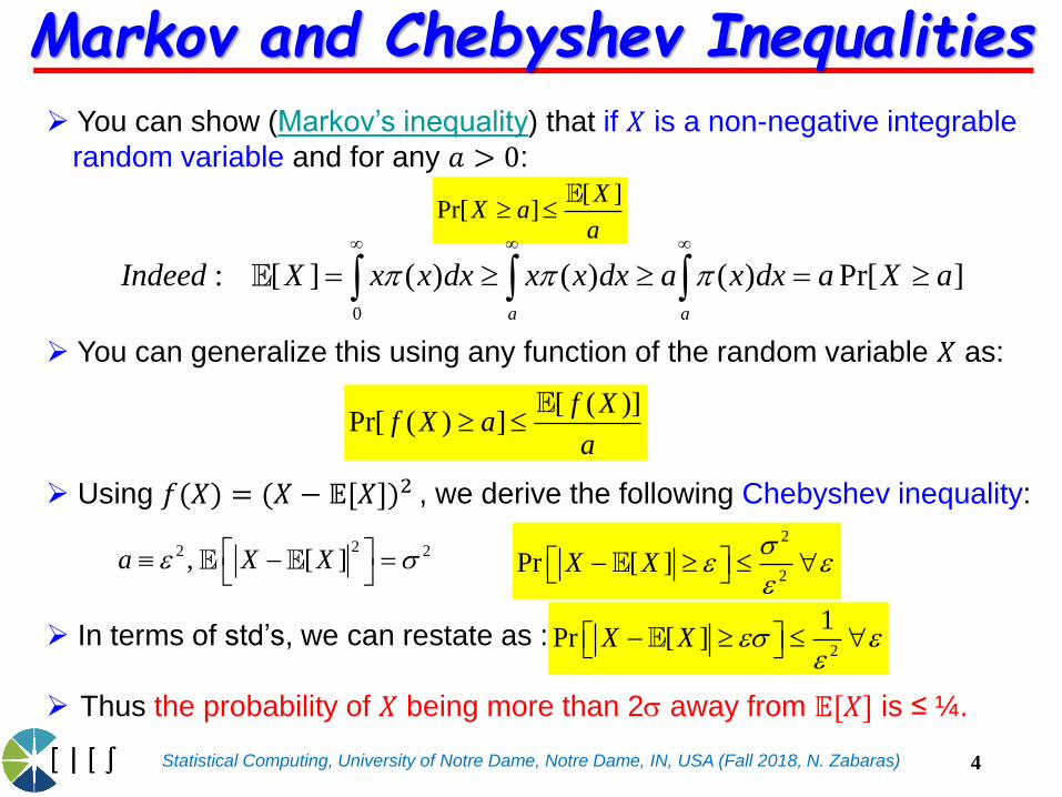
You can show (Markov’s inequality) that if 𝑋 is a non-negative integrable

random variable and for any 𝑎 > 0:

You can generalize this using any function of the random variable 𝑋 as:

Using 𝑓(𝑋) = (𝑋 − 𝔼[𝑋])2 , we derive the following Chebyshev inequality:

In terms of std’s, we can restate as :

Thus the probability of 𝑋 being more than 2s away from 𝔼[𝑋] is ≤ ¼.

[ ]Pr[ ]

XX a

a

2

2Pr [ ]X X

s

[ ( )]Pr[ ( ) ]

f Xf X a

a

22 2, [ ]a X X s

0

: [ ] ( ) ( ) ( ) Pr[ ]a a

Indeed X x x dx x x dx a x dx a X a

Markov and Chebyshev Inequalities

2

1Pr [ ]X X s

4

http://en.wikipedia.org/wiki/Markov's_inequality


Let 𝑋𝑖 for 𝑖 = 1, 2, . . . , 𝑛 be independent and identically distributed random variables (i.i.d.) with finite mean E(𝑋𝑖) = 𝜇 & variance Var(𝑋𝑖) =

𝜎2.

Let

Note that

Weak LLN:

Strong LLN:

The Law of Large Numbers (LLN)

This means that with

probability one, the

average of any

realizations of 𝑥1, 𝑥2, … of

the random variables

𝑋1, 𝑋2, … converges to

the mean.

ത𝑋𝑛 =1

𝑛

𝑖=1

𝑛

𝑋𝑖

𝔼 ത𝑋𝑛 =1

𝑛

𝑖=1

𝑛

𝜇 = 𝜇

𝑉𝑎𝑟 ത𝑋𝑛 =1

𝑛2

𝑖=1

𝑛

𝜎2 =𝜎2

𝑛

lim𝑛→∞

Pr | ത𝑋𝑛 − 𝜇| ≥ 𝜀 = 0∀𝜀 > 0

lim𝑛→∞

ത𝑋𝑛 = 𝜇 𝑎𝑙𝑚𝑜𝑠𝑡 𝑠𝑢𝑟𝑒𝑙𝑦

5


Assume that we have a set of observations

The problem is to infer on the underlying probability distribution that gives

rise to the data S.

1 2{ , ,... }, n

N jS x x x x

Parametric problem: The underlying probability density has a

specified known form that depends on a number of parameters. The

problem of interest is to infer those parameters.

Non-parametric problem: No analytical expression for the probability

density is available. Description consists of defining the dependency

or independency of the data. This leads to numerical exploration.

A typical situation for the parametric model is when the distribution is the

PDF of a random variable : .nX

Statistical Inference: Parametric & Non-Parametric Approach

6


Assume that we sample

We consider a parametric model with xj realizations of

where we take both the mean and the variance as

unknowns.

The probability density of 𝑋 is:

Our problem is to estimate and

2

1 2{ , ,... },N jS x x x x

0~ ( , )X x N

0x 2 2

1

0 0 01/2

1 1( | , ) exp ( ) ( )

22 det

Tx x x x x x

0x 2 2

Example of the Law of Large Numbers

7


From the law of large numbers, we calculate:

To compute the covariance matrix, note that if 𝑋1, 𝑋2, … are i.i.d. so are

𝑓(𝑋1), 𝑓(𝑋2), … for any function

Then we can compute:

The above formulas define the empirical mean and empirical

covariance.

2: kf

Empirical Mean and Empirical Covariance

𝑥0 = 𝔼 𝑋 ≈1

𝑁

𝑗=1

𝑁

𝑥𝑗 = ҧ𝑥

𝜮 = cov(𝑋) = 𝔼 ൫𝑥 − 𝔼 𝑋 ) 𝑥 − 𝔼 𝑋 𝑇 ≈ 𝔼 ൫𝑥 − ҧ𝑥) 𝑥 − ҧ𝑥 𝑇

⇒

𝜮 ≈1

𝑁

𝑗=1

𝑁

(𝑥𝑗 − ҧ𝑥) 𝑥𝑗 − ҧ𝑥𝑇= ഥ𝜮

8


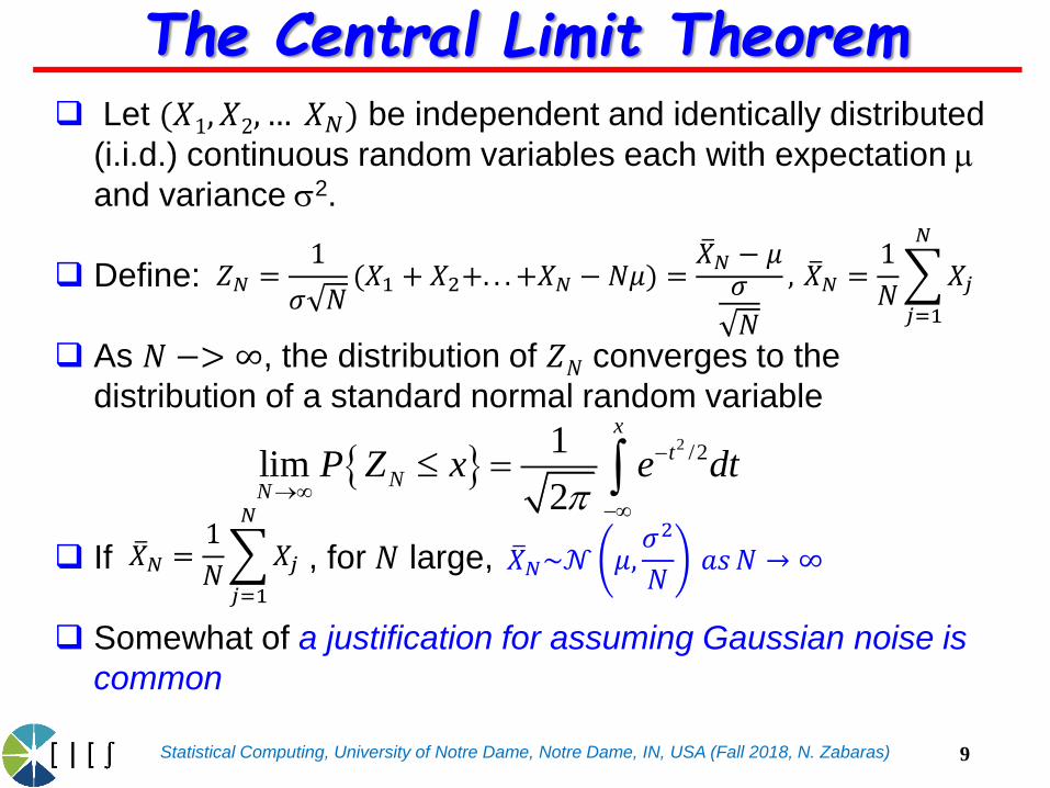
The Central Limit Theorem Let (𝑋1, 𝑋2, … 𝑋𝑁) be independent and identically distributed

(i.i.d.) continuous random variables each with expectation m

and variance s2.

Define:

As 𝑁 −> ∞, the distribution of 𝑍𝑁 converges to the

distribution of a standard normal random variable

If , for 𝑁 large,

Somewhat of a justification for assuming Gaussian noise is

common

2 /21

lim2

x

t

NN

P Z x e dt

𝑍𝑁 =1

𝜎 𝑁(𝑋1 + 𝑋2+. . . +𝑋𝑁 − 𝑁𝜇) =

ത𝑋𝑁 − 𝜇𝜎

𝑁

, ത𝑋𝑁 =1

𝑁

𝑗=1

𝑁

𝑋𝑗

ത𝑋𝑁 =1

𝑁

𝑗=1

𝑁

𝑋𝑗 ത𝑋𝑁~𝒩 𝜇,𝜎2

𝑁𝑎𝑠𝑁 → ∞

9


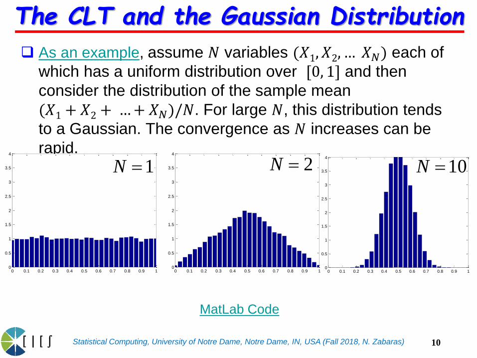
The CLT and the Gaussian Distribution

As an example, assume 𝑁 variables (𝑋1, 𝑋2, … 𝑋𝑁) each of

which has a uniform distribution over [0, 1] and then

consider the distribution of the sample mean

(𝑋1 + 𝑋2 + …+ 𝑋𝑁)/𝑁. For large 𝑁, this distribution tends

to a Gaussian. The convergence as 𝑁 increases can be

rapid.

0 0.1 0.2 0.3 0.4 0.5 0.6 0.7 0.8 0.9 10

0.5

1

1.5

2

2.5

3

3.5

4

0 0.1 0.2 0.3 0.4 0.5 0.6 0.7 0.8 0.9 10

0.5

1

1.5

2

2.5

3

3.5

4

0 0.1 0.2 0.3 0.4 0.5 0.6 0.7 0.8 0.9 10

0.5

1

1.5

2

2.5

3

3.5

4

MatLab Code

1N 2N 10N

10

http://www.zabaras.com/Courses/BayesianComputing/Software/Fig6Chapter2Bishop.m

https://www.dropbox.com/s/anm2xqg9ox9z2qi/Fig6Chapter2Bishop.m?dl=0


0 0.5 10

1

2

3

N = 10

The CLT and the Gaussian Distribution

We plot a histogram of where

As 𝑁 → ∞, the distribution tends towards a Gaussian.

0 0.5 10

1

2

3

N = 1

0 0.5 10

1

2

3

N = 5

1

1, 1:10000

N

ij

i

x jN

~ (1,5)ijx Beta

Run centralLimitDemo

from PMTK

11

https://github.com/probml/pmtk3/blob/master/demos/centralLimitDemo.m

https://github.com/probml/pmtk3


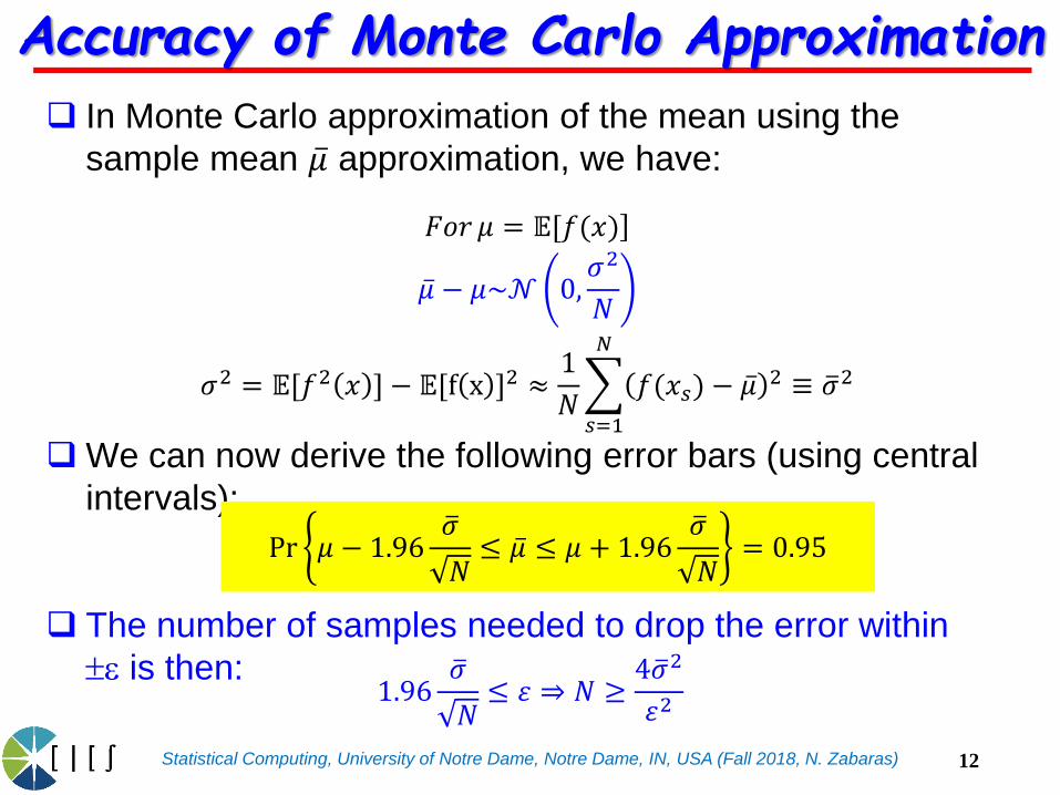
Accuracy of Monte Carlo Approximation

In Monte Carlo approximation of the mean using the

sample mean ҧ𝜇 approximation, we have:

We can now derive the following error bars (using central

intervals):

The number of samples needed to drop the error within

is then:

]𝐹𝑜𝑟 𝜇 = 𝔼[𝑓(𝑥)

ҧ𝜇 − 𝜇~𝒩 0,𝜎2

𝑁

𝜎2 = 𝔼[𝑓2 𝑥 ] − 𝔼[f x ]2 ≈1

𝑁

𝑠=1

𝑁

𝑓(𝑥𝑠) − ҧ𝜇 2 ≡ ത𝜎2

Pr 𝜇 − 1.96ത𝜎

𝑁≤ ҧ𝜇 ≤ 𝜇 + 1.96

ത𝜎

𝑁= 0.95

1.96ത𝜎

𝑁≤ 𝜀 ⇒ 𝑁 ≥

4ത𝜎2

𝜀2

12


Monte Carlo Approximation of Distributions

Computing the distribution of 𝑦 = 𝑥2, 𝑝(𝑥) is uniform.

The MC approximation is shown on the right. Take

samples from 𝑝(𝑥), square them and then plot the

histogram.

Run changeofVarsDemo1d

from PMTK

-1 0 1-0.5

0

0.5

1

1.5

0 0.5 10.5

1

1.5

2

2.5

3

3.5

4

4.5

5

5.5

0 0.5 10

0.05

0.1

0.15

0.2

0.25

𝑝(𝑥)

𝑝(𝑦)

13

https://github.com/probml/pmtk3/blob/master/demos/changeOfVarsDemo1d.m



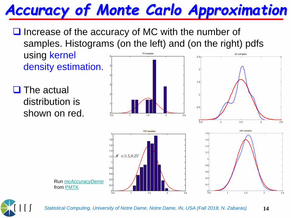
Accuracy of Monte Carlo Approximation

Increase of the accuracy of MC with the number of

samples. Histograms (on the left) and (on the right) pdfs

using kernel

density estimation.

The actual

distribution is

shown on red.

Run mcAccuracyDemo

from PMTK0.5 1 1.5 2 2.50

0.2

0.4

0.6

0.8

1

1.2

1.4

1.6

1.8100 samples

0.5 1 1.5 2 2.50

0.5

1

1.5

2

2.510 samples

2|1.5,0.25xN

14

https://github.com/probml/pmtk3/blob/master/demos/mcAccuracyDemo.m



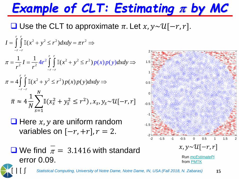
Example of CLT: Estimating by MC

Use the CLT to approximate 𝜋. Let 𝑥, 𝑦~𝒰[−𝑟, 𝑟].

Here 𝑥, 𝑦 are uniform random

variables on [−𝑟,+𝑟], 𝑟 = 2.

We find = 3.1416with standard

error 0.09. Run mcEstimatePi

from PMTK

-2 -1.5 -1 -0.5 0 0.5 1 1.5 2-2

-1.5

-1

-0.5

0

0.5

1

1.5

2

2 2 2 2

22 2 2

2 2

2 2 2

4 (

( )

1 1( )

4 ( )

) (

( )

)

( )

r r

r r

r r

r r

r r

r r

I x y r dxdy r

I x y r dxdyr r

x y r p x p y dxd

r p p

y

x y

ത𝜋 ≈ 41

𝑁

𝑠=1

𝑁

)𝕀(𝑥𝑠2 + 𝑦𝑠

2 ≤ 𝑟2 , 𝑥𝑠, 𝑦𝑠~𝒰[−𝑟, 𝑟]

15

𝑥, 𝑦~𝒰[−𝑟, 𝑟]

https://github.com/probml/pmtk3/blob/master/demos/mcEstimatePi.m



CLT: The Binomial Tends to a Gaussian

One consequence of the CLT is that the binomial

distribution

which is a distribution over m defined by the sum of 𝑁observations of the random binary variable 𝑥, will tend to a

Gaussian as 𝑁 → ∞.

| , (1 )m N mN

m Nm

Bin

0 1 2 3 4 5 6 7 8 9 100

0.05

0.1

0.15

0.2

0.25

0.3

0.35binomial distribution

( 10, 0.25)N m Bin

Matlab Code

16

1 2

~

1...

,

~ ,

1

Nx x x m

N N N

m N NN

N

https://www.dropbox.com/s/yq6ewb0ekqpapbi/Fig1Chapter2Bishop.m?dl=0


Consider that we count the number of photons from a light source. Let

𝑁(𝑡) be the number of photons observed in the time interval [0, 𝑡]. 𝑁(𝑡) is

an integer-valued random variable. We make the following assumptions:

a. Stationarity: Let ∆1 and ∆2 be any two time intervals of equal length, 𝑛any non-negative integer. Assume that

Prob. of 𝑛 photons in ∆1= Prob. of 𝑛 photons in ∆2

b. Independent increments: Let ∆1, ∆2, … , ∆𝑛 be non-overlapping time

intervals and 𝑘1, 𝑘2, … , 𝑘𝑛 non-negative integers. Denote by 𝐴𝑗 the event

defined as

𝐴𝑗 = 𝑘𝑗 photons arrive in the time interval ∆𝑗

Assume that these events are mutually independent, i.e.

c. Negligible probability of coincidence: Assume that the probability of

two or more events at the same time is negligible. More precisely,

𝑁(0) = 0 and

1 2 1 2( ... ) ( ) ( )... ( )n nP A A A P A P A P A

( ) 1lim 0

P N h

h

0h

Poisson Process

17


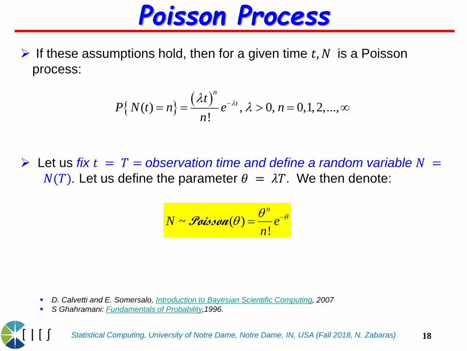
If these assumptions hold, then for a given time 𝑡, 𝑁 is a Poisson

process:

Let us fix 𝑡 = 𝑇 = observation time and define a random variable 𝑁 =𝑁(𝑇). Let us define the parameter 𝜃 = 𝜆𝑇. We then denote:

( ) , 0, 0,1,2,...,!

n

tt

P N t n e nn

~ ( )!

n

N en

Poisson

Poisson Process

18

D. Calvetti and E. Somersalo, Introduction to Bayesian Scientific Computing, 2007

S Ghahramani: Fundamentals of Probability,1996.

http://www.amazon.com/Introduction-Bayesian-Scientific-Computing-Mathematical/dp/0387733930

http://www.amazon.com/Fundamentals-Probability-2nd-Saeed-Ghahramani/dp/0130113298


Consider the Poisson (discrete) distribution

The mean and the variance are both equal to .

( ) ( | )!

n

PoissonP N n n en

0

2

( | ) ,Poisson

n

N n n

N

Poisson Process

19

0,1,2,...,N


Approximating a Poisson Distribution With a Gaussian

Theorem: A random variable 𝑋~Poisson(𝜃) can be considered as the

sum of n independent random variables 𝑋𝑖~Poisson(𝜃/𝑛).a

According to the Central Limit Theorem, when 𝑛 is large enough,

Then based on the Theorem is a draw from and

from the CLT also follows a Gaussian for large n with:

Thus

The approximation of a Poisson distribution with a Gaussian for large

𝑛 is a result of the CLT!

a For a proof that the sum of independent Poisson Random Variables is a Poisson distribution see this document.

21

1~ ( , ) ~ ( , )

n

i i

i

Take X Xn n n n n

Poisson N

1

n

i

i

X X

2

2

X nn

var X nn

~ ( , ) X N

20

)𝒫ℴ𝒾𝓈𝓈ℴ𝓃(𝜃

https://www.dropbox.com/s/5t470kf5y2jiulf/convol.pdf?dl=0


Approximating a Poisson Distribution with a Gaussian

0 2 4 6 8 10 12 14 16 18 200

0.02

0.04

0.06

0.08

0.1

0.12

0.14

0.16

0.18

Mean=5

0 2 4 6 8 10 12 14 16 18 200

0.02

0.04

0.06

0.08

0.1

0.12

0.14

Mean=10

0 5 10 15 20 25 30 35 40 45 500

0.02

0.04

0.06

0.08

0.1

0.12

Mean=15

0 5 10 15 20 25 30 35 40 45 500

0.01

0.02

0.03

0.04

0.05

0.06

0.07

0.08

0.09

Mean=20

21

Poisson distributions (dots) vs their Gaussian approximations (solid line) for various values of the

mean . The higher the , the smaller the distance between the two distributions. See this MatLab

implementation.

https://www.dropbox.com/s/k9niovgnxfn4hjk/PoissonVsGaussian.rar?dl=0


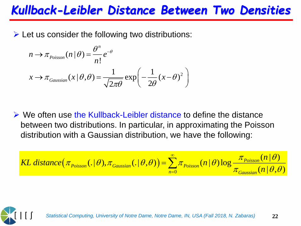
Let us consider the following two distributions:

We often use the Kullback-Leibler distance to define the distance

between two distributions. In particular, in approximating the Poisson

distribution with a Gaussian distribution, we have the following:

0

( | )(. | ), (. | , ) ( | ) log

( | , )

PoissonPoisson Gaussian Poisson

n Gaussian

nKL distance n

n

2

( | )!

1 1( | , ) exp ( )

22

n

Poisson

Gaussian

n n en

x x x

Kullback-Leibler Distance Between Two Densities

22


0 5 10 15 20 25 30 35 40 45 5010

-3

10-2

10-1

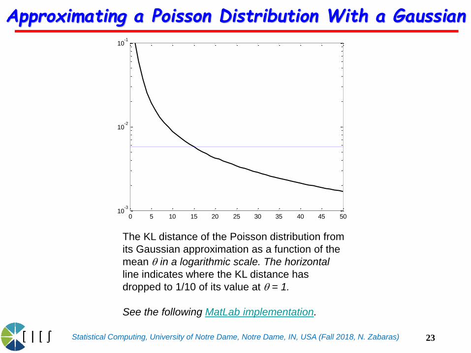
Approximating a Poisson Distribution With a Gaussian

23

The KL distance of the Poisson distribution from

its Gaussian approximation as a function of the

mean in a logarithmic scale. The horizontal

line indicates where the KL distance has

dropped to 1/10 of its value at = 1.

See the following MatLab implementation.

https://www.dropbox.com/s/5hguz2pmolndq9d/KLdist.m?dl=0


Consider discrete sampling where the output is noise of length 𝑛.

The noise vector is a realization of

We estimate the mean and the variance of the noise in a single measurement

as follows:

To improve the signal to noise ratio, we repeat the measurement and average

the noise vector signals:

The average noise is a realization of a random variable:

If are i.i.d., X is asymptotically a Gaussian by the CLT, and its

variance is . We need to repeat the experiment until

(a given tolerance).

nx : nX

2

2

0 0

1 1

1 1,

n n

j j

j j

x x x xn n

s

( )

1

1 Nk n

k

x xN

( )

1

1 Nk n

k

X XN

2

var( )XN

s

(1) (2), ,...X X

22

Ns

Application of the CLT: Noise Signals

24


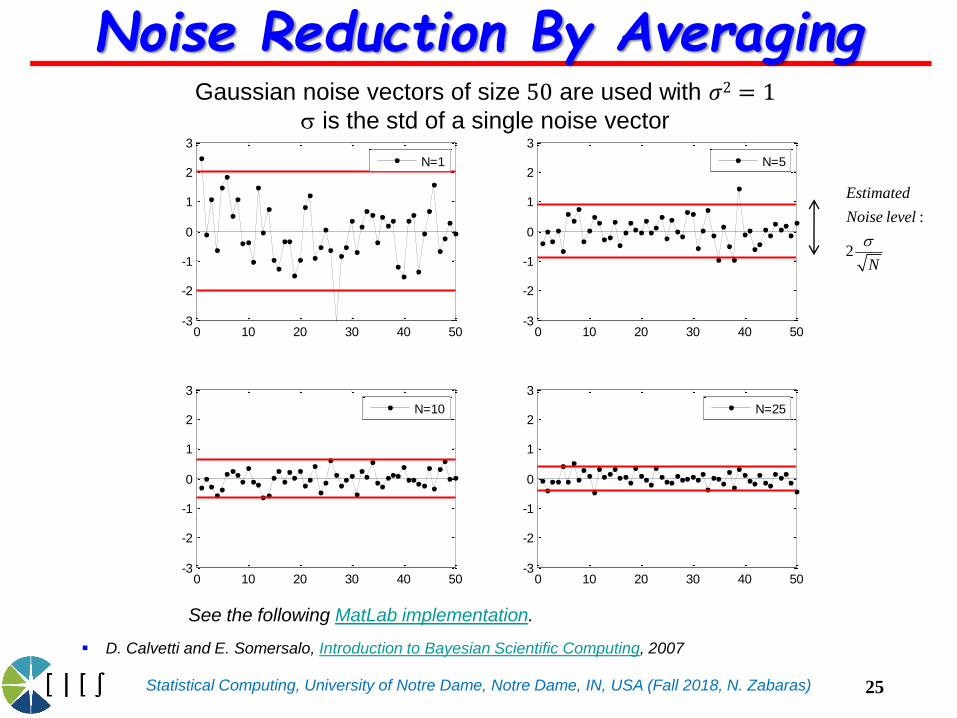
Gaussian noise vectors of size 50 are used with 𝜎2 = 1s is the std of a single noise vector

0 10 20 30 40 50-3

-2

-1

0

1

2

3

N=1

0 10 20 30 40 50-3

-2

-1

0

1

2

3

N=5

0 10 20 30 40 50-3

-2

-1

0

1

2

3

N=10

0 10 20 30 40 50-3

-2

-1

0

1

2

3

N=25

Noise Reduction By Averaging

25

:

2

Estimated

Noise level

N

s

See the following MatLab implementation.

D. Calvetti and E. Somersalo, Introduction to Bayesian Scientific Computing, 2007

https://www.dropbox.com/s/5f5etc70l3q8cq2/AveragedNoiseSignals.m?dl=0

http://www.amazon.com/Introduction-Bayesian-Scientific-Computing-Mathematical/dp/0387733930


Information theory is concerned

with representing data in a compact fashion (data

compression or source coding), and

transmitting and storing it in a way that is robust to

errors (error correction or channel coding).

To compactly representing data requires allocating

short codewords to highly probable bit strings, and

reserving longer codewords to less probable bit strings.

e.g. in natural language, common words (“a”, “the”,

“and”) are much shorter than rare words.

Introduction to Information Theory

D. MacKay, Information Theory, Inference and Learning Algorithms (Video Lectures)

26

compactly representing

http://videolectures.net/course_information_theory_pattern_recognition/


Decoding messages sent over noisy channels requires

having a good probability model of the kinds of

messages that people tend to send.

We need models that can predict which kinds of data

are likely and which unlikely.


• David MacKay, Information Theory, Inference and Learning Algorithms , 2003 (available on line)

• Thomas M. Cover, Joy A. Thomas , Elements of Information Theory , Wiley, 2006.

• Viterbi, A. J. and J. K. Omura (1979). Principles of Digital Communication and Coding. McGraw-Hill.

27

http://www.inference.phy.cam.ac.uk/mackay/

http://www.inference.phy.cam.ac.uk/mackay/itila/

http://www.amazon.com/s/ref=ntt_athr_dp_sr_1?_encoding=UTF8&field-author=Thomas M. Cover&search-alias=books&sort=relevancerank

http://www.amazon.com/s/ref=ntt_athr_dp_sr_2?_encoding=UTF8&field-author=Joy A. Thomas&search-alias=books&sort=relevancerank

http://www.amazon.com/Elements-Information-Theory-Telecommunications-Processing/dp/0471062596

https://archive.org/details/principledigcom00viterich


Consider a discrete random variable 𝑥. We ask how

much information (‘degree of surprise’) is received when

we observe (learn) a specific value for this variable?

Observing a highly probable event provides little

additional information.

If we have two events 𝑥 and 𝑦 that are unrelated, then

the information gain from observing both of them should

be ℎ(𝑥, 𝑦) = ℎ(𝑥) + ℎ(𝑦).

Two unrelated events will be statistically independent, so

𝑝(𝑥, 𝑦) = 𝑝(𝑥)𝑝(𝑦).


28


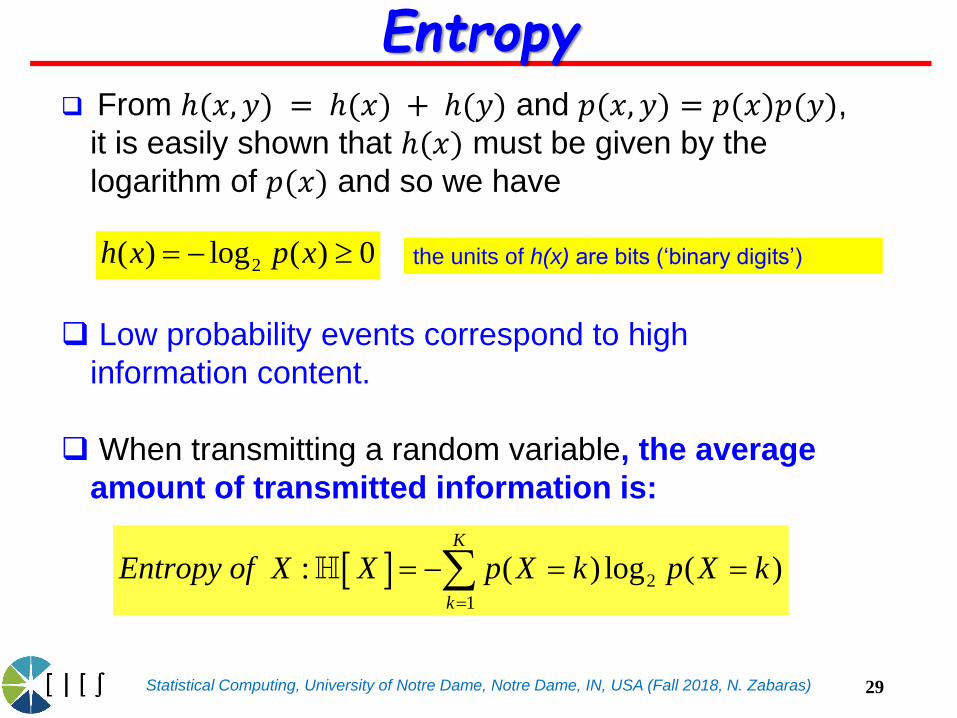
From ℎ(𝑥, 𝑦) = ℎ(𝑥) + ℎ(𝑦) and 𝑝(𝑥, 𝑦) = 𝑝(𝑥)𝑝(𝑦), it is easily shown that ℎ(𝑥) must be given by the

logarithm of 𝑝(𝑥) and so we have

Low probability events correspond to high

information content.

When transmitting a random variable, the average

amount of transmitted information is:

the units of h(x) are bits (‘binary digits’)2( ) log ( ) 0h x p x

2

1

: ( ) log ( )K

k

Entropy of X X p X k p X k

Entropy

29


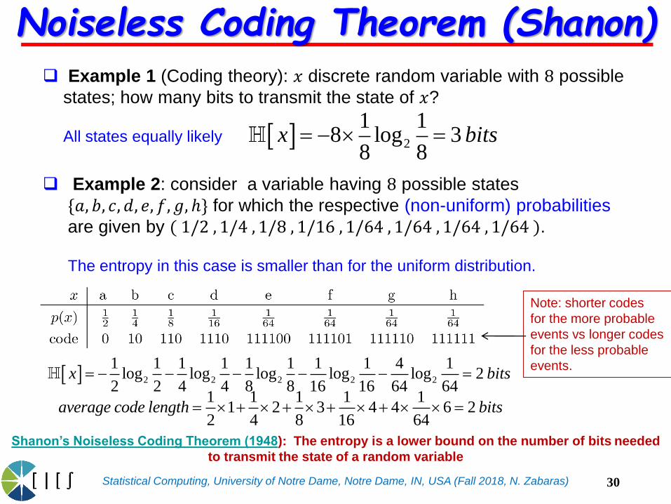
Example 1 (Coding theory): 𝑥 discrete random variable with 8 possible

states; how many bits to transmit the state of 𝑥?

All states equally likely

Example 2: consider a variable having 8 possible states

{𝑎, 𝑏, 𝑐, 𝑑, 𝑒, 𝑓, 𝑔, ℎ} for which the respective (non-uniform) probabilities

are given by ( 1/2 , 1/4 , 1/8 , 1/16 , 1/64 , 1/64 , 1/64 , 1/64 ).

The entropy in this case is smaller than for the uniform distribution.

2

1 18 log 3

8 8x bits

1 1 1 1 11 2 3 4 4 6 2

2 4 8 16 64average code length bits

2 2 2 2 2

1 1 1 1 1 1 1 1 4 1log log log log log 2

2 2 4 4 8 8 16 16 64 64x bits

Note: shorter codes

for the more probable

events vs longer codes

for the less probable

events.

Shanon’s Noiseless Coding Theorem (1948): The entropy is a lower bound on the number of bits needed

to transmit the state of a random variable

Noiseless Coding Theorem (Shanon)

30

http://en.wikipedia.org/wiki/Shannon's_source_coding_theorem


Considering a set of 𝑁 identical objects that are to be divided

amongst a set of bins, such that there are 𝑛𝑖 objects in the ith bin.

Consider the number of different ways of allocating the objects to

the bins.

In the ith bin there are 𝑛𝑖! ways of reordering the objects

(microstates), and so the total number of ways of allocating the 𝑁objects to the bins is given by (multiplicity)

The entropy is defined as

We now consider the limit 𝑁 →∞,

!

!i

i

NW

n

1 1 1

ln ln ! ln !iiW N n

N N N

ln ! ln , ln ! lni i i iN N N N n n n n

lim ln lni ii i

Ni i

n np p

N N

pi is the probability of an object assigned

to the ith bin.

The occupation numbers pi correspond

to macrostates.

Alternative Definition of Entropy

31


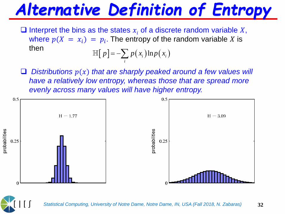
Interpret the bins as the states 𝑥𝑖 of a discrete random variable 𝑋,

where 𝑝(𝑋 = 𝑥𝑖) = 𝑝𝑖. The entropy of the random variable 𝑋 is

then

Alternative Definition of Entropy

Distributions 𝑝(𝑥) that are sharply peaked around a few values will

have a relatively low entropy, whereas those that are spread more

evenly across many values will have higher entropy.

lni i

i

p p x p x

32


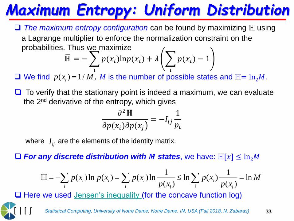
The maximum entropy configuration can be found by maximizing H using

a Lagrange multiplier to enforce the normalization constraint on the

probabilities. Thus we maximize

We find 𝑀 is the number of possible states and H= ln2𝑀.

To verify that the stationary point is indeed a maximum, we can evaluate

the 2nd derivative of the entropy, which gives

For any discrete distribution with 𝑴 states, we have: H[𝑥] ≤ ln2𝑀

Here we used Jensen’s inequality (for the concave function log)

where are the elements of the identity matrix.ijI

( ) 1/ ,ip x M

Maximum Entropy: Uniform Distribution

1 1( ) ln ( ) ( ) ln ln ( ) ln

( ) ( )i i i i

i i ii i

p x p x p x p x Mp x p x

ഥℍ = −

𝑖

𝑝(𝑥𝑖)ln𝑝(𝑥𝑖) + 𝜆

𝑖

𝑝(𝑥𝑖) − 1

𝜕2ഥℍ

൯𝜕𝑝(𝑥𝑖)𝜕𝑝(𝑥𝑗= −𝐼𝑖𝑗

1

𝑝𝑖

33

https://en.wikipedia.org/wiki/Jensen's_inequality


Recall the DNA Sequence logo example earlier.

The height of each bar is defined to be 2 − H, where H is

the entropy of that distribution, and 2 (= ln24) is the

maximum possible entropy.

Thus a bar of height 0corresponds to a uniform

distribution (ln24), whereas

a bar of height 2 corresponds

to a deterministic distribution.

Example: Biosequence Analysis

1 2 3 4 5 6 7 8 9 10 11 12 13 14 150

1

2

Sequence Position

Bit

s

seqlogoDemo from PMTK

34

https://github.com/probml/pmtk3/blob/master/demos/seqlogoDemo.m



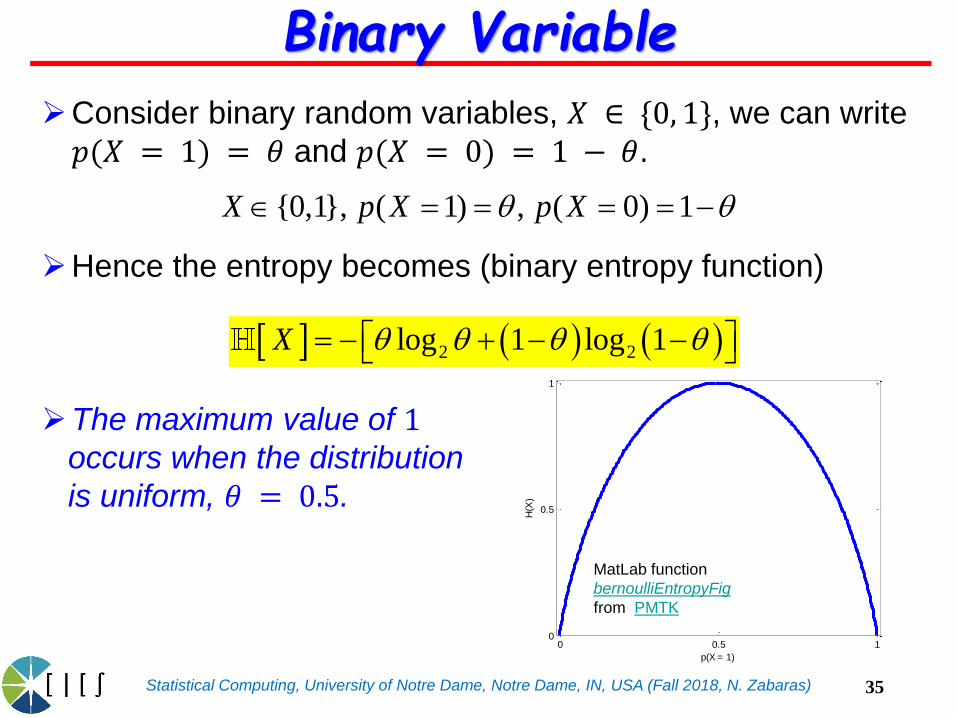
Consider binary random variables, 𝑋 ∈ {0, 1}, we can write

𝑝(𝑋 = 1) = 𝜃 and 𝑝(𝑋 = 0) = 1 − 𝜃.

Hence the entropy becomes (binary entropy function)

The maximum value of 1occurs when the distribution

is uniform, 𝜃 = 0.5.

Binary Variable

{0,1}, ( 1) , ( 0) 1X p X p X

2 2log 1 log 1X

0 0.5 10

0.5

1

p(X = 1)

H(X

)

MatLab function

bernoulliEntropyFig

from PMTK

35

https://github.com/probml/pmtk3/blob/master/demos/bernoulliEntropyFig.m



Divide 𝑥 into bins of width Δ. Assuming 𝑝(𝑥) is

continuous, for each such bin, there must exist 𝑥𝑖 such

that

The ln Δ term is omitted since it diverges as Δ0(indicating that infinite bits are needed to describe a

continuous variable)

( 1)

0

( ) ( )

( ) ln ( ) ( ) ln ( ) ln

lim ( ) ln ( ) ( ) ln ( )

i

i

i

i i i i

i i

i i

i

p x dx p x =

p x p x p x p x

p x p x p x p x dx

probability in falling in bin

(can be negative)

Differential Entropy

36


For a density defined over multiple continuous

variables, denoted collectively by the vector 𝒙, the

differential entropy is given by

Differential (unlike the discrete) entropy can be negative

When doing variable transformation 𝒚(𝒙), use 𝑝(𝒙)𝑑𝒙 =𝑝(𝒚)𝑑𝒚, e.g. if 𝒚 = 𝑨𝒙 then:

( ) ln ( )p p d x x x x

Differential Entropy

( ) ln ( ) | | l | | n | |n lp p d yx y y A y A x Ay

37


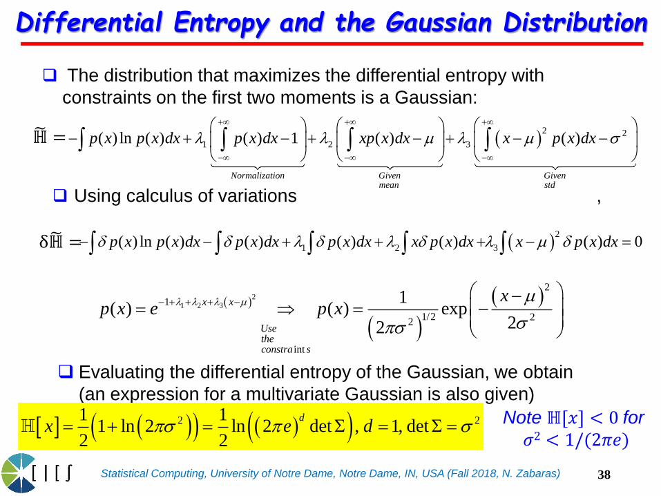
The distribution that maximizes the differential entropy with

constraints on the first two moments is a Gaussian:

Using calculus of variations ,

Evaluating the differential entropy of the Gaussian, we obtain

(an expression for a multivariate Gaussian is also given)

2 21 11 ln 2 ln 2 det , 1, det

2 2

dx e ds s

21 2 3

2

1

1/2 22

int

1( ) ( ) exp

22

x x

Usetheconstra s

xp x e p x

m m

ss

2 2

1 2 3( ) ln ( ) ( ) 1 ( ) ( )

Normalization Given Givenmean std

p x p x dx p x dx xp x dx x p x dx m m s

Differential Entropy and the Gaussian Distribution

Note ℍ[𝑥] < 0 for

𝜎2 < 1/(2𝜋𝑒)

2

1 2 3( ) ln ( ) ( ) ( ) ( ) ( ) 0p x p x dx p x dx p x dx x p x dx x p x dx m

෩ℍ =

δ෩ℍ =

38


Consider some unknown distribution 𝑝(𝑥), and suppose

that we have modeled this using an approximating

distribution 𝑞(𝑥).

If we use 𝑞(𝑥) to construct a coding scheme for the

purpose of transmitting values of 𝑥 to a receiver, then the

additional information to specify 𝑥 is:

The cross entropy is defined as:

( )|| ( ) ln ( ) ( ) ln ( ) ( ) ln

( )

q xKL p q p x q x dx p x p x dx p x dx

p x

I transmit q(x) butI average it with theexact probability p(x)

Kullback-Leibler Divergence and Cross Entropy

, ( ) ln ( )p q p x q x dx

39


The cross entropy is the average

number of bits needed to encode data coming from a

source with distribution p when we use model q to define

our codebook.

H(𝑝)=H(𝑝, 𝑝) is the expected # of bits using the true model.

The KL divergence is the average number of extra bits

needed to encode the data, because we used distribution q

to encode the data instead of the true distribution p.

The “extra number of bits” interpretation makes it clear that

KL(p||q) ≥ 0, and that the KL is only equal to zero iff q = p.

The KL distance is not a symmetrical quantity, that is

( )|| ( ) ln ( ) ( ) ln ( ) ( ) ln

( )

q xKL p q p x q x dx p x p x dx p x dx

p x

KL Divergence and Cross Entropy

|| ||KL p q KL q p

40

, ( ) ln ( )p q p x q x dx


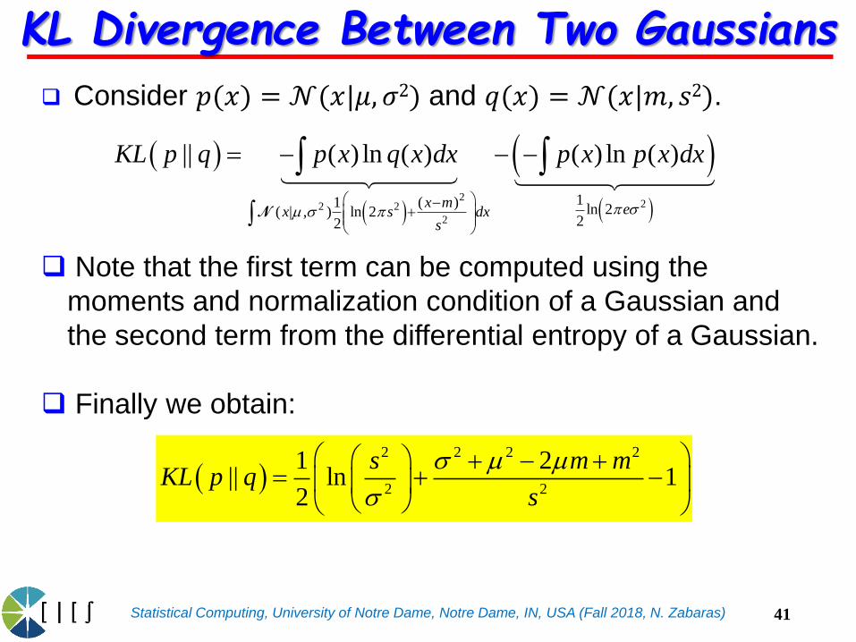
Consider 𝑝(𝑥) = 𝒩(𝑥|𝜇, 𝜎2) and 𝑞(𝑥) = 𝒩(𝑥|𝑚, 𝑠2).

Note that the first term can be computed using the

moments and normalization condition of a Gaussian and

the second term from the differential entropy of a Gaussian.

Finally we obtain:

222 2

2

11 ( ) ln 2( | , ) ln 222

|| ( ) ln ( ) ( ) ln ( )

x m ex s dxs

KL p q p x q x dx p x p x dx

sm s

N

KL Divergence Between Two Gaussians

2 2 2 2

2 2

1 2|| ln 1

2

s m mKL p q

s

s m m

s

41


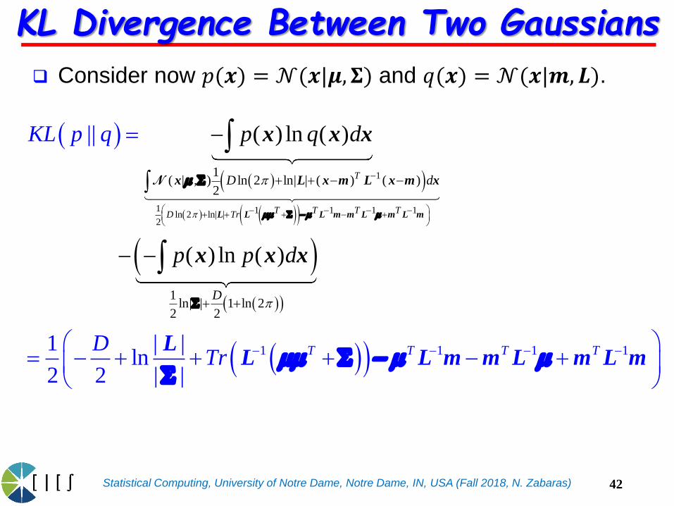
Consider now 𝑝(𝒙) = 𝒩(𝒙|𝝁, 𝚺) and 𝑞(𝒙) = 𝒩(𝒙|𝒎, 𝑳).

1

1 1 1 1 1ln 2 ln| |2

1( | , ) ln 2 ln| | ( ) ( )

2

1ln| | 1 ln 2

2 2

( ) ln ( )

( ) ln

||

1 | |ln

2

(

2 | |

)

T

T T T TD Tr

D d

D

KL p q

D

p q d

p p d

N

L L L m m L m L m

x L x m L x m x

x x x

x

L

x x

mm m m

m

1 1 1 1T T T TTr

L L m m L m L mmm m m

KL Divergence Between Two Gaussians

42


For a convex function 𝑓, Jensen’s inequality gives (can

be proven easily by induction)

This is equivalent (assume 𝑀 = 2)

to our requirement for convexity 𝑓”(𝑥) > 0.

Assume 𝑓”(𝑥) > 0 (strict convexity) for any 𝑥.

Jensen’s inequality is thus shown:

1 1

( ), 0 1M M

i i i i i i

i i i

f x f x and

Jensen’s Inequality

0

2

0 0 0 0 0 0 0

0 0 0

0 0 0

0 0 0 :

1( ) ( ) '( )( ) "( *)( ) ( ) '( )( )

2

( ) ( ) '( )( ), : ( ) (1 ) ( ) ( ) '( )( (1 ) )

( ) ( ) '( )( )Set x

f x f x f x x x f x x x f x f x x x

f a f x f x a xFor x a b f a f b f x f x a b x

f b f x f x b x

( ) (1 ) ( ) (1 )f a f b f a b

43


Assume Jensen’s inequality. We should show that

𝑓”(𝑥) > 0 (strict convexity) for any 𝑥.

Set the following: 𝑎 = 𝑏 − 2𝜀, 𝑏 = 𝑎 + 2𝜀 > 𝑎, 𝜀 > 0.

Using Jensen’s inequality, we can easily derive the

above equation as:

For small, we thus have:


( ) ( ) ( ) ( )'( ) '( ) (.)

f b f b f a f aor f b f a f is convex

1 1( ) ( ) 0.5 0.5

2 2

1 10.5( 2 ) 0.5 0.5 0.5( 2 )

2 2

1 1( ) ( ) ( ) ( ) ( ) ( )

2 2

f a f b f a b

f b b f a a

f b f a f b f b f a f a

44


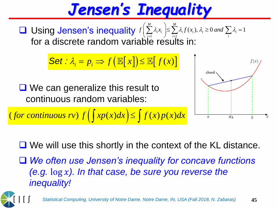
Using Jensen’s inequality

for a discrete random variable results in:

We can generalize this result to

continuous random variables:

We will use this shortly in the context of the KL distance.

We often use Jensen’s inequality for concave functions

(e.g. log 𝑥). In that case, be sure you reverse the

inequality!

1 1

( ), 0 1M M

i i i i i i

i i i

f x f x and

( ) ( ) ( ) ( )for continuous rv f xp x dx f x p x dx


( )i ip f x f x Set :

45


As another example of Jensen’s inequality, consider the

arithmetic and geometric means of a set of real variables:

Using Jensen’s inequality for 𝑓(𝑥) = log(𝑥) (concave),

i.e.

, we can show:

Jensen’s Inequality: Example

ҧ𝑥𝐴 =1

𝑀

𝑖=1

𝑀

𝑥𝑖 , ҧ𝑥𝐺 = ෑ

𝑖=1

𝑀

𝑥𝑖

Τ1 𝑀

ln ҧ𝑥𝐺 =1

𝑀ln ෑ

𝑖=1

𝑀

𝑥𝑖 =

𝑖=1

𝑀

1

𝑀ln𝑥𝑖 ≤ ln

𝑖=1

𝑀

1

𝑀𝑥𝑖 = ln ҧ𝑥𝐴 ⇒ ҧ𝑥𝐺 ≤ ҧ𝑥𝐴

ln( ) lnx x

46


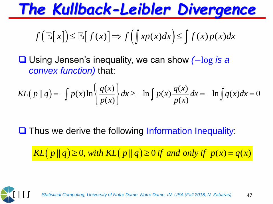
Using Jensen’s inequality, we can show (−log is a

convex function) that:

Thus we derive the following Information Inequality:

|| 0, || 0 ( ) ( )KL p q with KL p q if and only if p x q x

( ) ( ) ( ) ( )f x f x f xp x dx f x p x dx

( ) ( )

|| ( ) ln ln ( ) ln ( ) 0( ) ( )

q x q xKL p q p x dx p x dx q x dx

p x p x

The Kullback-Leibler Divergence

47


An important consequence of the information inequality is

that the discrete distribution with the maximum entropy is

the uniform distribution.

More precisely, ℍ(𝑋) ≤ log |𝒳 |, where | 𝒳 | is the

number of states for 𝑋, with equality iff 𝑝(𝑥) is uniform. To

see this, let 𝑢(𝑥) = 1/ | 𝒳 |. Then

This principle of insufficient reason, argues in favor of

using uniform distributions when there are no other

reasons to favor one distribution over another.

|| ( ) log ( ) ( ) log ( ) log | | ( ) 0x x

KL p u p x u x p x p x x X

Principle of Insufficient Reason

48


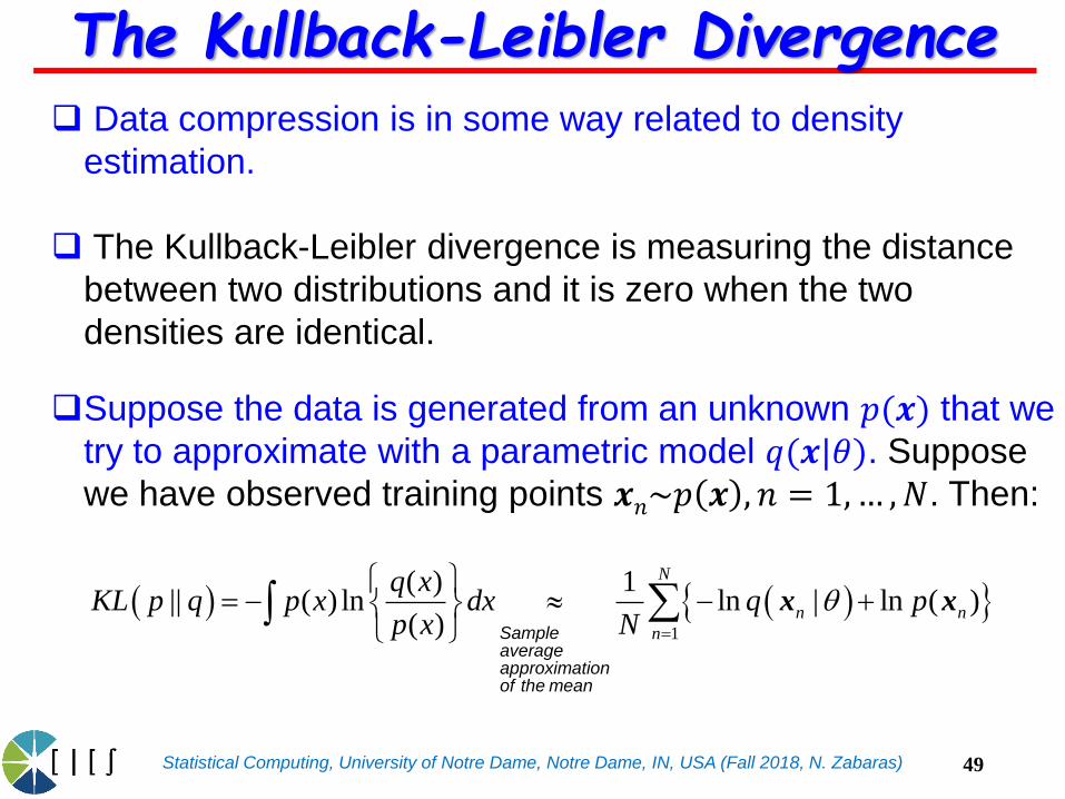
Data compression is in some way related to density

estimation.

The Kullback-Leibler divergence is measuring the distance

between two distributions and it is zero when the two

densities are identical.

Suppose the data is generated from an unknown 𝑝(𝒙) that we

try to approximate with a parametric model 𝑞(𝒙|𝜃). Suppose

we have observed training points 𝒙𝑛~𝑝 𝒙 , 𝑛 = 1,… ,𝑁. Then:

1

( ) 1|| ( ) ln ln | ln ( )

( )

N

n n

n

q xKL p q p x dx q p

p x N

x x

Sampleaverageapproximationof the mean

The Kullback-Leibler Divergence

49


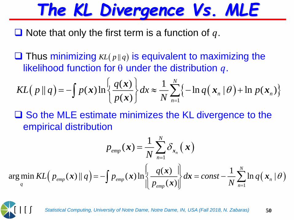
Note that only the first term is a function of 𝑞.

Thus minimizing is equivalent to maximizing the

likelihood function for under the distribution 𝑞.

So the MLE estimate minimizes the KL divergence to the

empirical distribution

1

( ) 1|| ( ) ln ln | ln ( )

( )

N

n n

n

qKL p q p dx q p

p N

xx x x

x

||KL p q

The KL Divergence Vs. MLE

1

1( )

n

N

emp

n

pN

xx x

1

( ) 1arg min ( ) || ( ) ln ln |

( )

N

emp emp nq nemp

qKL p q p d const q

p N

xx x x x

x

50


For a joint distribution, the conditional entropy is

This represents the average information to specify 𝑦 if we

already know the value of 𝑥

It is easily seen, using , and substituting

inside the log in that the

conditional entropy satisfies the relation

where H[𝑥, 𝑦] is the differential entropy of 𝑝(𝑥, 𝑦)and H[𝑥] is the differential entropy of 𝑝(𝑥).

, |x y y x x

| ( , ) ln ( | )y x p y x p y x dydx

Conditional Entropy

( , ) ( | ) ( )p y x p y x p x

, ( , ) ln ( , )x y p x y p x y dydx

51


Consider the conditional entropy for discrete variables

To understand further the meaning of conditional entropy,let us consider the implications of H[𝑦|𝑥] = 0.

We have:

From this we can conclude that

Since 𝑝𝑙𝑜𝑔𝑝 = 0 ↔ 𝑝 = 0 or 𝑝 = 1 and since 𝑝(𝑦𝑖|𝑥𝑗) is

normalized, there is only one 𝑦𝑖 s.t. with all

other . Thus 𝑦 is a function of 𝑥.

| ( , ) ln ( | )i j i j

i j

y x p y x p y x

Conditional Entropy for Discrete Variables

0

| ( | ) ln ( | ) ( ) 0i j i j j

i j

y x p y x p y x p x

: ( | ) ln ( | ) 0i j i jthe following must hold p y x p y x

( | ) 1i jp y x

. . ( ) 0j jFor each x s t p x

(. | ) 0jp x

52


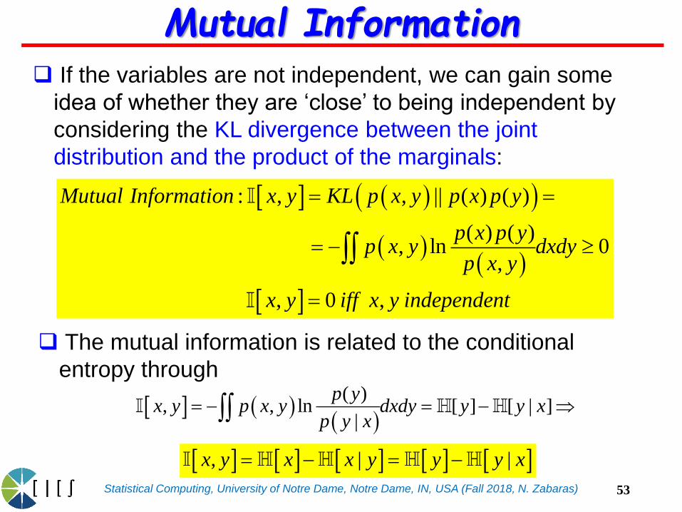
If the variables are not independent, we can gain some

idea of whether they are ‘close’ to being independent by

considering the KL divergence between the joint

distribution and the product of the marginals:

The mutual information is related to the conditional

entropy through

, | |x y x x y y y x

: , , || ( ) ( )

( ) ( ), ln 0

,

, 0 ,

Mutual Information x y KL p x y p x p y

p x p yp x y dxdy

p x y

x y iff x y independent

Mutual Information

( )

, , ln [ ] [ | ]|

p yx y p x y dxdy y y x

p y x

53


The mutual information represents the reduction in the

uncertainty about 𝑥 once we learn the value of 𝑦 (and

reversely).

In a Bayesian setting, 𝑝(𝑥) =prior, 𝑝(𝑥|𝑦) posterior, and I[𝑥, 𝑦] represents the reduction in uncertainty in 𝑥 once

we observe 𝑦.

, | |x y x x y y y x

Mutual Information

H y

|

|

x x y

y y x

54


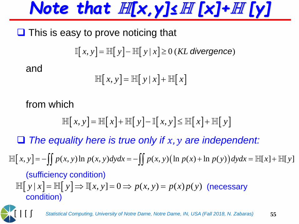
This is easy to prove noticing that

and

from which

The equality here is true only if 𝑥, 𝑦 are independent:

(sufficiency condition)

(necessary

condition)

, | 0 ( )x y y y x KL divergence

Note that H[x,y]≤H [x]+H [y]

, |x y y x x

, ,x y x y x y x y

, ( , ) ln ( , ) ( , ) ln ( ) ln ( ) [ ] [ ]x y p x y p x y dydx p x y p x p y dydx x y

| [ , ] 0 ( , ) ( ) ( )y x y x y p x y p x p y

55


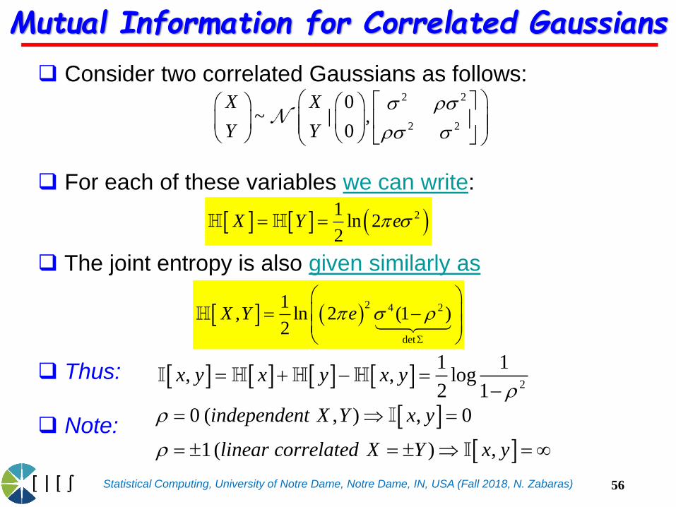
Consider two correlated Gaussians as follows:

For each of these variables we can write:

The joint entropy is also given similarly as

Thus:

Note:

2 2

2 2

0~ | ,

0

X X

Y Y

s s

s s

Mutual Information for Correlated Gaussians

2

1 1, , log

2 1x y x y x y

21ln 2

2X Y e s

2 4 2

det

1, ln 2 (1 )

2X Y e s

0 ( , ) , 0

1 ( ) ,

independent X Y x y

linear correlated X Y x y

56

https://en.wikipedia.org/wiki/Normal_distribution

https://en.wikipedia.org/wiki/Multivariate_normal_distribution


A quantity which is closely related to 𝑀𝐼 is the pointwise

mutual information or 𝑃𝑀𝐼. For two events (not random

variables) 𝑥 and 𝑦, this is defined as

This measures the discrepancy between these events

occurring together compared to what would be expected

by chance. Clearly the 𝑀𝐼, , of 𝑋 and 𝑌 is just the

expected value of the 𝑃𝑀𝐼.

This is the amount we learn from updating the prior 𝑝(𝑥)into the posterior 𝑝(𝑥|𝑦), or equivalently, updating the

prior 𝑝(𝑦) into the posterior 𝑝(𝑦|𝑥).

Pointwise Mutual Information

( ) ( ) ( | ) ( | )

( , ) : log log log, ( ) ( )

p x p y p x y p y xPMI x y

p x y p x p y

57

,x y


For continuous random variables, it is common to first

discretize or quantize them into bins, and computing

how many values fall in each histogram bin (Scott 1979).

The number of bins used, and the location of the bin

boundaries, can have a significant effect on the results.

One can estimate the 𝑀𝐼 directly, without performing

density estimation (Learned-Miller, 2004). Another

approach is to try many different bin sizes and locations,

and to compute the maximum 𝑀𝐼 achieved.

Mutual Information

Scott, D. (1979). On optimal and data-based histograms, Biometrika 66(3), 605–610.

Learned-Miller, E. (2004). Hyperspacings and the estimation of information theoretic quantities. Technical Report

04-104, U. Mass. Amherst Comp. Sci. Dept.

Reshef, D., Y. Reshef, H. Finucane, S. Grossman, G. McVean, P. Turnbaugh, E. Lander, M. Mitzenmacher, and P.

Sabeti (2011, December). Detecting novel associations n large data sets. Science 334, 1518–1524.

Speed, T. (2011, December). A correlation for the 21st century. Science 334, 152–1503.

*Use MatLab function miMixedDemo from Kevin Murphys’ PMTK

58

http://biomet.oxfordjournals.org/content/66/3/605.short

https://www.dropbox.com/s/0gee2xnn8ddtcco/Scott1979.pdf?dl=0

http://biomet.oxfordjournals.org/content/66/3/605.short

https://people.cs.umass.edu/~elm/papers_by_area.html

https://www.dropbox.com/s/o6otv1njyki2rkl/LearnedMiller2004.pdf?dl=0

https://people.cs.umass.edu/~elm/papers/04-104.pdf

https://www.dropbox.com/s/i6nuwf9f0vvhcxy/Science-2011-Reshef-1518-24.pdf?dl=0

http://www.sciencemag.org/content/334/6062/1518

https://www.dropbox.com/s/hcrg36q7vde5f02/Speed2011.pdf?dl=0


https://code.google.com/p/pmtk3/source/browse/trunk/demos/bookDemos/Information_theory/miMixedDemo.m?r=2660

https://code.google.com/p/pmtk3/


This statistic appropriately normalized is known as the

maximal information coefficient (𝑀𝐼𝐶).

We first define:

Here G (𝑥, 𝑦) is the set of 2𝑑 grids of size , and

𝑋(𝐺), 𝑌 (𝐺) represents a discretization of the variables

onto this grid (The maximization over bin locations is

performed efficiently using dynamic programming)

Now define the 𝑀𝐼𝐶 as

Maximal Information Coefficient

( , )max ( ); ( )( , )

log min( , )

G x y X G Y Gm x y

x y

G

, :max ( , )

x y xy BMIC m x y



x y

59




The 𝑀𝐼𝐶 is defined as:

𝐵 is some sample-size dependent bound on the number

of bins we can use and still reliably estimate the

distribution (Reshef et al. suggest 𝐵 ~ 𝑁0.6).

𝑀𝐼𝐶 lies in the range [0, 1], where 0 represents no

relationship between the variables, and 1 represents a

noise-free relationship of any form, not just linear.

Maximal Information Coefficient

( , )max ( ); ( )( , )

log min( , )

G x y X G Y Gm x y

x y

G

, :max ( , )

x y xy BMIC m x y



60




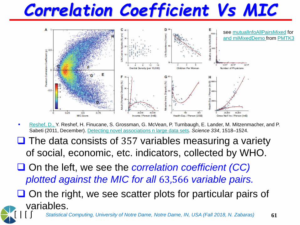
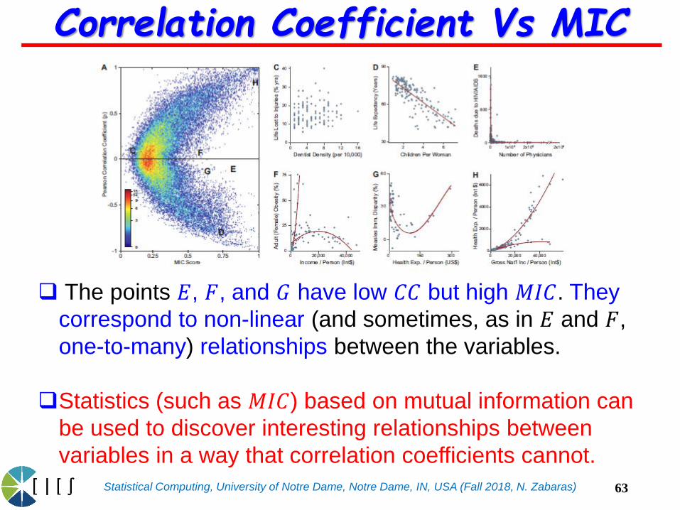
The data consists of 357 variables measuring a variety

of social, economic, etc. indicators, collected by WHO.

On the left, we see the correlation coefficient (CC)

plotted against the MIC for all 63,566 variable pairs.

On the right, we see scatter plots for particular pairs of

variables.

Correlation Coefficient Vs MIC



see mutualInfoAllPairsMixed for

and miMixedDemo from PMTK3

61



https://github.com/probml/pmtk3/blob/master/matlabTools/stats/mutualInfoAllPairsMixed.m

https://github.com/probml/pmtk3/blob/master/demos/miMixedDemo.m



Point marked 𝐶 has a low 𝐶𝐶 and a low 𝑀𝐼𝐶. From the

corresponding scatter we see that there is no relationship

between these two variables.

The points marked 𝐷 and 𝐻 have high 𝐶𝐶 (in absolute

value) and high 𝑀𝐼𝐶 and we see from the scatter plot that

they represent nearly linear relationships.


62


The points 𝐸, 𝐹, and 𝐺 have low 𝐶𝐶 but high 𝑀𝐼𝐶. They

correspond to non-linear (and sometimes, as in 𝐸 and 𝐹,

one-to-many) relationships between the variables.

Statistics (such as 𝑀𝐼𝐶) based on mutual information can

be used to discover interesting relationships between

variables in a way that correlation coefficients cannot.


63

Introduction to Probability and Statistics (Continued)Introduction to Probability and Statistics...

Documents

Transcript of Introduction to Probability and Statistics (Continued)Introduction to Probability and Statistics...