Introduction to Probability and Statistics Chapter 8 Large-Sample Estimation.

Introduction to Probability Introduction to Probability and Statisticsand Statistics

Chapter 8

Large-Sample Estimation

IntroductionIntroduction• Populations and parameters

– For a normal populationpopulation mean and s.d.

– A binomial populationpopulation proportion p

• If parameters are unknown, we make inferences about them using sample information.

Inferential StatisticsInferential StatisticsInferential StatisticsInferential Statistics

Types of InferenceTypes of Inference• Estimation:Estimation:

– Estimating the value of the parameter– “What is (are) the values of or p?”

• Hypothesis Testing:Hypothesis Testing: – Deciding about the value of a parameter

based on some preconceived idea.– “Did the sample come from a population

with or p = .2?”

Types of InferenceTypes of Inference• Examples:Examples:

– A consumer wants to estimate the average price of similar homes in her city before putting her home on the market.

Estimation:Estimation: Estimate , the average home price.Estimation:Estimation: Estimate , the average home price.

Hypothesis testHypothesis test: Is the new average resistance, equal to the old average resistance,

Hypothesis testHypothesis test: Is the new average resistance, equal to the old average resistance,

– A manufacturer wants to know if a new type of steel is more resistant to high temperatures than an old type was.

Types of InferenceTypes of Inference

• Whether estimating parameters or testing hypotheses, statistical methods of inferential statistics are to:

– Make statistical inference

– Tell goodness or reliability of the inference

DefinitionsDefinitions

• An estimatorestimator is a rule, usually a formula, that tells you how to calculate the estimate based on the sample.

• Estimators are calculated from sample observations, hence they are statistics.– Point estimation: Point estimation: A single number is

calculated to estimate the parameter.– Interval estimation:Interval estimation: Two numbers are

calculated to create an interval within which the parameter is expected to lie.

““Good” Point EstimatorsGood” Point Estimators

• An estimatorestimator is unbiasedunbiased if the mean of its sampling distribution equals the parameter of interest.– It does not systematically overestimate

or underestimate the target parameter.– Sample mean is an unbiased estimator

of population mean.– Sample proportion is an unbiased

estimator of population proportion.

““Good” Point EstimatorsGood” Point Estimators

• Of all the unbiasedunbiased estimators, we prefer the estimator whose sampling distribution has the smallest spreadsmallest spread or variability,variability, i.e. smallest standard deviation or standard error.

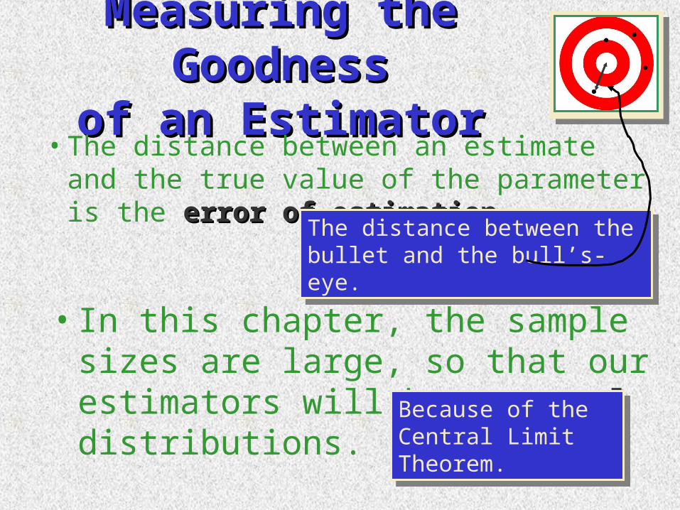
Measuring the GoodnessMeasuring the Goodnessof an Estimatorof an Estimator

• The distance between an estimate and the true value of the parameter is the error of error of estimation.estimation. The distance between the bullet and

the bull’s-eye.

The distance between the bullet and the bull’s-eye.

• In this chapter, the sample sizes are large, so that our estimators will have normal normal distributions. Because of the Central

Limit Theorem.

Because of the Central Limit Theorem.

The Margin of ErrorThe Margin of Error

• For unbiased estimators with normal sampling distributions, 95% of all point estimates will lie within 1.96 standard deviations of the parameter of interest.

estimator theof S96.1 E estimator theof S96.1 E

• 95%Margin of error: 95%Margin of error: The maximum error of estimation, calculated as

Estimating Means Estimating Means and Proportionsand Proportions

•For a quantitative population,

n

sn

xμ

96.1 :)30(error ofMargin

:mean population ofestimator Point

n

sn

xμ

96.1 :)30(error ofMargin

:mean population ofestimator Point

•For a binomial population,

n

qpqnpn

x/npp

ˆˆ96.1 :)5ˆ,5ˆ(error ofMargin

ˆ : proportion population ofestimator Point

n

qpqnpn

x/npp

ˆˆ96.1 :)5ˆ,5ˆ(error ofMargin

ˆ : proportion population ofestimator Point

ExampleExample• A homeowner randomly samples 64 homes

similar to her own and finds that the average selling price is $252,000 with a standard deviation of $15,000.

• Estimate the average selling price for all similar homes in the city.

Point estimator of : 252,000

15,000Margin of error : 1.96 1.96 3675

64

μ x

s

n

Point estimator of : 252,000

15,000Margin of error : 1.96 1.96 3675

64

μ x

s

n

ExampleExampleA quality control technician wants to estimate the proportion of soda cans that are underfilled. He randomly samples 200 cans of soda and finds 10 underfilled cans.

03.200

)95)(.05(.96.1

ˆˆ96.1

05.200/10ˆ

200

n

qp

x/npp

pn

:error of Margin

: ofestimator Point

cans dunderfille of proportion

03.200

)95)(.05(.96.1

ˆˆ96.1

05.200/10ˆ

200

n

qp

x/npp

pn

:error of Margin

: ofestimator Point

cans dunderfille of proportion

Interval EstimationInterval Estimation• Create an interval (a, b) so that you are fairly

sure that the parameter lies between these two values. Confidence IntervalConfidence Interval

Usually, 1-

Usually, 1-• Suppose 1- = .95 and

that the estimator has a normal distribution.

Parameter 1.96SEParameter 1.96SE

• “Fairly sure” means “with high probability”, measured using the confidence coefficient, 1confidence coefficient, 1

Interval EstimationInterval Estimation• Since we don’t know the value of the parameter,

consider which has a variable center.

• Only if the estimator falls in the tails will the interval fail to enclose the parameter. This happens only 5% of the time.

Estimator 1.96SEEstimator 1.96SE

WorkedWorkedWorked

Failed

To Change the Confidence To Change the Confidence LevelLevel

• To change to a general confidence level, 1-, pick a value of z that puts area 1-in the center of the z distribution.

100(1-)% Confidence Interval:

Estimator zSE

100(1-)% Confidence Interval:

Estimator zSE

Tail area z/2 1-.05 1.645 .90

.025 1.96 .95

.01 2.33 .98

.005 2.58 .99

Confidence Intervals Confidence Intervals for Means and Proportionsfor Means and Proportions• For a Quantitative Population

n

szx

μ

2/

:Mean Population afor Interval Confidence

n

szx

μ

2/

:Mean Population afor Interval Confidence

• For a Binomial Population

n

qpzp

p

ˆˆˆ

: Proportion Populationfor Interval Confidence

2/n

qpzp

p

ˆˆˆ

: Proportion Populationfor Interval Confidence

2/

ExampleExample

• A random sample of n = 50 males showed a mean average daily intake of dairy products equal to 756 grams with a standard deviation of 35 grams. Find a 95% confidence interval for the population average

n

sx 96.1

50

3596.17 56 70.97 56

grams. 65.70 746.30or 7

ExampleExample

• Find a 99% confidence interval for the population average daily intake of dairy products for men.

n

sx 58.2

50

3558.27 56 77.127 56

grams. 7 743.23or 77.68 The interval must be wider to provide for the increased confidence that it does indeed enclose the true value of .

ExampleExample• Of a random sample of n = 150 college students,

104 of the students said that they had played on a soccer team during their K-12 years.

• Estimate p, the proportion of college students who played soccer in their youth with a 98% confidence interval.

n

qpp

ˆˆ33.2ˆ

150

)31(.69.33.2

104

150

09.. 69 .60or .78. p

Estimating the Difference Estimating the Difference between Two Meansbetween Two Means

• Sometimes we are interested in comparing the means of two populations.

•The average growth of plants fed using two different nutrients.•The average scores for students taught with two different teaching methods.

• To make this comparison,

. varianceand mean with 1 population

fromdrawn size of sample randomA 211

1

μ

n



1

μ

n



2

μ

n



2

μ

n

Estimating the Difference Estimating the Difference between Two Meansbetween Two Means

•We compare the two averages by making inferences about -, the difference in the two population averages.

•If the two population averages are the same, then 1-= 0.•The best estimate of 1-is the difference in the two sample means,

21 xx 21 xx

The Sampling The Sampling Distribution of Distribution of 1 2x x

.SE as

estimated becan SE and normal,ely approximat is of

ondistributi sampling thelarge, are sizes sample theIf .3

.SE is ofdeviation standard The 2.

means. population the

in difference the, is ofmean The 1.

2

22

1

21

21

2

22

1

21

21

2121

n

s

n

s

xx

nnxx

xx

.SE as

estimated becan SE and normal,ely approximat is of


.SE is ofdeviation standard The 2.

means. population the

in difference the, is ofmean The 1.

2

22

1

21

21

2

22

1

21

21

2121

n

s

n

s

xx

nnxx

xx

Estimating Estimating 11--

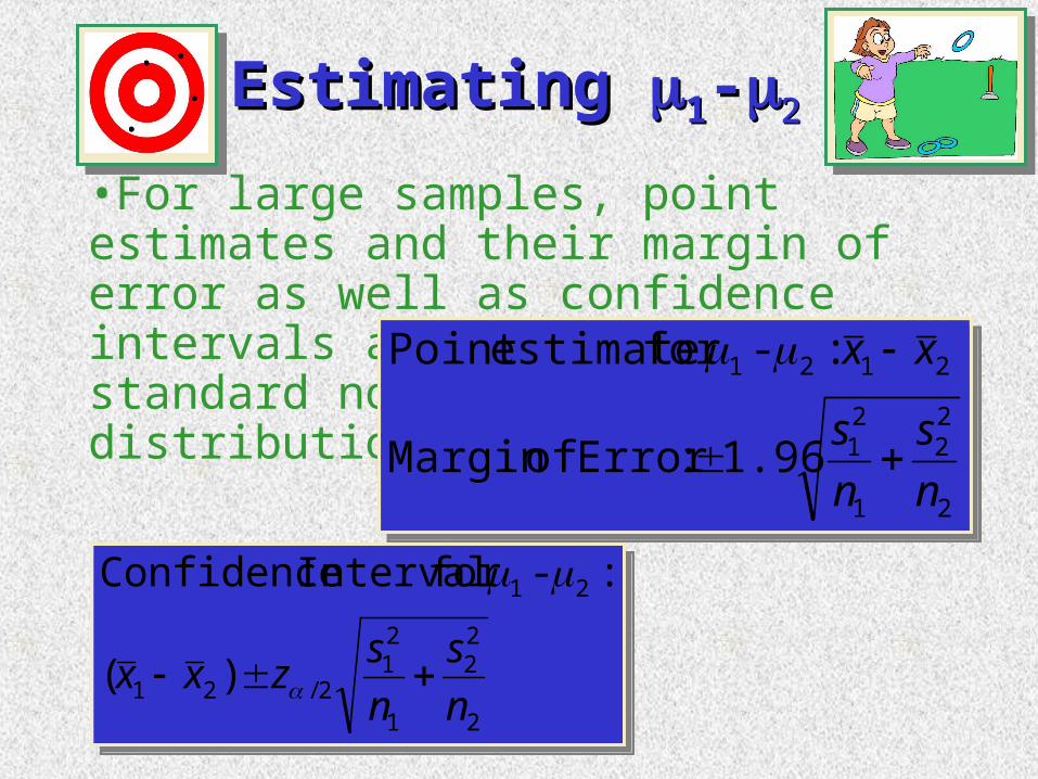
•For large samples, point estimates and their margin of error as well as confidence intervals are based on the standard normal (z) distribution.

2

22

1

21

2121

1.96 :Error ofMargin

:-for estimatePoint

n

s

n

s

xx

2

22

1

21

2121

1.96 :Error ofMargin

:-for estimatePoint

n

s

n

s

xx

2

22

1

21

2/21

21

)(

:-for Interval Confidence

n

s

n

szxx

2

22

1

21

2/21

21

)(

:-for Interval Confidence

n

s

n

szxx

ExampleExample

• Compare the average daily intake of dairy products of men and women using a 95% confidence interval.

78.126

.78.6 18.78-or 21

Avg Daily Intakes Men Women

Sample size 50 50

Sample mean 756 762

Sample Std Dev 35 30

2

22

1

21

21 96.1)(n

s

n

sxx

2 235 30(756 762) 1.96

50 50

Example, continuedExample, continued

• Could you conclude, based on this confidence interval, that there is a difference in the average daily intake of dairy products for men and women?

• The confidence interval contains the value 11--= 0= 0.. Therefore, it is possible that 11 = = You would not want to conclude that there is a difference in average daily intake of dairy products for men and women.

78.6 18.78- 21 78.6 18.78- 21

Estimating the Difference Estimating the Difference between Two Proportionsbetween Two Proportions

•Sometimes we are interested in comparing the proportion of “successes” in two binomial populations.

•The germination rates of untreated seeds and seeds treated with a fungicide.•The proportion of male and female voters who favor a particular candidate for governor.

•To make this comparison,

.parameter with 1 population binomial

fromdrawn size of sample randomA

1

1

p

n.parameter with 1 population binomial


1

1

p

n

.parameter with 2 population binomial


2

2

p

n.parameter with 2 population binomial


2

2

p

n

Estimating the Difference Estimating the Difference between Two Proportionsbetween Two Proportions

•We compare the two proportions by making inferences about p-p, the difference in the two population proportions.

•If the two population proportions are the same, then p1-p= 0.•The best estimate of p1-pis the difference in the two sample proportions,

2

2

1

121 ˆˆ

n

x

n

xpp

2

2

1

121 ˆˆ

n

x

n

xpp

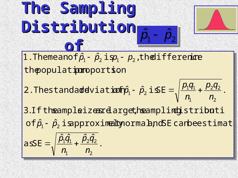
The Sampling The Sampling Distribution of Distribution of

.ˆˆˆˆ

SE as

estimated becan SE and normal,ely approximat is ˆˆ of


.SE is ˆˆ ofdeviation standard The 2.

s.proportion population the

in difference the, is ˆˆ ofmean The 1.

2

22

1

11

21

2

22

1

1121

2121

n

qp

n

qp

pp

n

qp

n

qppp

pppp

.ˆˆˆˆ

SE as

estimated becan SE and normal,ely approximat is ˆˆ of


.SE is ˆˆ ofdeviation standard The 2.

s.proportion population the

in difference the, is ˆˆ ofmean The 1.

2

22

1

11

21

2

22

1

1121

2121

n

qp

n

qp

pp

n

qp

n

qppp

pppp

21 ˆˆ pp 21 ˆˆ pp

Estimating Estimating pp11--pp

•For large samples, point estimates and their margin of error as well as confidence intervals are based on the standard normal (z) distribution.

2

22

1

11

2121

ˆˆˆˆ1.96 :Error ofMargin

ˆˆ :for estimatePoint

n

qp

n

qp

pp-pp

2

22

1

11

2121

ˆˆˆˆ1.96 :Error ofMargin

ˆˆ :for estimatePoint

n

qp

n

qp

pp-pp

2

22

1

112/21

21

ˆˆˆˆ)ˆˆ(

:for interval Confidence

n

qp

n

qpzpp

pp

2

22

1

112/21

21

ˆˆˆˆ)ˆˆ(

:for interval Confidence

n

qp

n

qpzpp

pp

ExampleExample

• Compare the proportion of male and female college students who said that they had played on a soccer team during their K-12 years using a 99% confidence interval.

2

22

1

1121

ˆˆˆˆ58.2)ˆˆ(

n

qp

n

qppp

70

)44(.56.

80

)19(.81.58.2)

70

39

80

65( 19.52.

.44. .06or 21 pp

Youth Soccer Male Female

Sample size 80 70

Played soccer 65 39

Example, continuedExample, continued

• Could you conclude, based on this confidence interval, that there is a difference in the proportion of male and female college students who said that they had played on a soccer team during their K-12 years?

• The confidence interval does not contain the value pp11--pp= 0= 0.. Therefore, it is not likely that pp11= = ppYou would conclude that there is a difference in the proportions for males and females.

44. .06 21 pp 44. .06 21 pp

A higher proportion of males than females played soccer in their youth.

Key ConceptsKey ConceptsI. Types of EstimatorsI. Types of Estimators

1. Point estimator: a single number is calculated to estimate the population parameter.2. Interval estimatorInterval estimator: two numbers are calculated to form an interval that contains the parameter.

II. Properties of Good EstimatorsII. Properties of Good Estimators1. Unbiased: the average value of the estimator equals the parameter to be estimated.2. Minimum variance: of all the unbiased estimators, the best estimator has a sampling distribution with the smallest standard error.

Key ConceptsKey ConceptsIII. Large-Sample Point EstimatorsIII. Large-Sample Point Estimators

To estimate one of four population parameters when the sample sizes are large, use the following point estimators with the appropriate margins of error.

Key ConceptsKey ConceptsIV. Large-Sample Interval EstimatorsIV. Large-Sample Interval Estimators

To estimate one of four population parameters when the sample sizes are large, use the following interval estimators.

Key ConceptsKey Concepts1. All values in the interval are possible values for

the unknown population parameter.2. Any values outside the interval are unlikely to be

the value of the unknown parameter.3. To compare two population means or proportions,

look for the value 0 in the confidence interval. If 0 is in the interval, it is possible that the two population means or proportions are equal, and you should not declare a difference. If 0 is not in the interval, it is unlikely that the two means or proportions are equal, and you can confidently declare a difference.

Introduction to Probability and Statistics Chapter 8 Large-Sample Estimation.

Documents

Transcript of Introduction to Probability and Statistics Chapter 8 Large-Sample Estimation.