Introduction to Probabilistic Graphical Modelspub.ist.ac.at/~chl/courses/PGM_W16/part9.pdf ·...
58
Energy Minimization (Integer) Linear Programming Local Search Sampling Sampling Loss functions Introduction to Probabilistic Graphical Models Christoph Lampert IST Austria (Institute of Science and Technology Austria) 1 / 40
Transcript of Introduction to Probabilistic Graphical Modelspub.ist.ac.at/~chl/courses/PGM_W16/part9.pdf ·...

Energy Minimization (Integer) Linear Programming Local Search Sampling Sampling Loss functions
Introduction to Probabilistic Graphical Models
Christoph Lampert
IST Austria (Institute of Science and Technology Austria)
1 / 40

Energy Minimization (Integer) Linear Programming Local Search Sampling Sampling Loss functions
Schedule
Refresher of ProbabilitiesIntroduction to Probabilistic Graphical Models
Probabilistic InferenceLearning Conditional Random Fields
MAP Prediction / Energy MinimizationLearning Structured Support Vector Machines
Links to slide download: http://pub.ist.ac.at/~chl/courses/PGM_W16/
Password for ZIP files (if any): pgm2016
Email for questions, suggestions or typos that you found: [email protected]
2 / 40

Energy Minimization (Integer) Linear Programming Local Search Sampling Sampling Loss functions
Supervised Learning Problem
I Given training examples (x1, y1), . . . , (xN , yN) ∈ X × Yx ∈ X : input, e.g. imagey ∈ Y: structured output, e.g. human pose, sentence
Images: HumanEva dataset
Goal: be able to make predictions for new inputs, i.e. learn a function f : X → Y.3 / 40

Energy Minimization (Integer) Linear Programming Local Search Sampling Sampling Loss functions
Supervised Learning Problem
Step 1: define a proper graph structure of X and Y
. . .
Ytop
Yhead
YtorsoYrarm
Yrhnd
Yrleg
Yrfoot Ylfoot
Ylleg
Ylarm
Ylhnd
X
. . .
. . .
. . .
. . .
. . .
. . .
. . .
. . .
. . .
. . .
F(1)
top
F(2)
top,head
Step 2: define a proper parameterization of p(y |x ; θ) p(y |x ; θ) =1
Ze∑d
i=1 θiφi (x ,y)
Step 3: learn parameters θ∗ from training data e.g. maximum likelihood
Step 4: for new x ∈ X , make predictione.g. y∗ = argmax
y∈Yp(y |x ; θ∗)
(→ today)
4 / 40

MAP Prediction / Energy Minimization
argmaxy p(y |x) / argminy E (y , x)
Energy Minimization (Integer) Linear Programming Local Search Sampling Sampling Loss functions
MAP Prediction / Energy Minimization
I Exact Energy Minimization
I Belief Propagation on chains/trees
I Graph-Cuts for submodular energies
I Integer Linear Programming
I Approximate Energy Minimization
I Linear Programming Relaxations
I Local Search Methods
I Iterative Conditional Modes
I Multi-label Graph Cuts
I Simulated Annealing
6 / 40

Energy Minimization (Integer) Linear Programming Local Search Sampling Sampling Loss functions
Example: Pictorial Structures / Deformable Parts Model
. . .
Ytop
Yhead
YtorsoYrarm
Yrhnd
Yrleg
Yrfoot Ylfoot
Ylleg
Ylarm
Ylhnd
X
. . .
. . .
. . .
. . .
. . .
. . .
. . .
. . .
. . .
. . .
F(1)
top
F(2)
top,head
I Tree-structured model for articulated pose(Felzenszwalb and Huttenlocher, 2000), (Fischler and Elschlager, 1973),
(Yang and Ramanan, 2013), (Pishchulin et al., 2012)
7 / 40

Energy Minimization (Integer) Linear Programming Local Search Sampling Sampling Loss functions
Example: Pictorial Structures / Deformable Parts Model
I most likely configuration y∗ = argmaxy∈Y
p(y |x) = argminy
E (y , x)
8 / 40

Energy Minimization (Integer) Linear Programming Local Search Sampling Sampling Loss functions
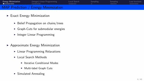
Energy Minimization – Belief Propagation
Chain model: same trick as for inference: belief propagation
miny
E (y) = minyi ,yj ,yk ,yl
EF (yi , yj) + EG (yj , yk) + EH(yk , yl)
= minyi ,yj
[EF (yi , yj) + min
yk
[EG (yj , yk) + min
ylEH(yk , yl)︸ ︷︷ ︸
rH→Yk(yk )
]]
= minyi ,yj
[EF (yi , yj) + min
ykEG (yj , yk) + rH→Yk
(yk)︸ ︷︷ ︸rG→Yj
(yj )
]
= minyi ,yj
[EF (yi , yj) + rG→Yj
(yj)]
. . .
I actual argmax by backtracking which choices were maximal
9 / 40

Energy Minimization (Integer) Linear Programming Local Search Sampling Sampling Loss functions
Energy Minimization – Belief Propagation
Chain model: same trick as for inference: belief propagation
miny
E (y) = minyi ,yj ,yk ,yl
EF (yi , yj) + EG (yj , yk) + EH(yk , yl)
= minyi ,yj
[EF (yi , yj) + min
yk
[EG (yj , yk) + min
ylEH(yk , yl)
]]
= minyi ,yj
[EF (yi , yj) + min
yk
[EG (yj , yk) + min
ylEH(yk , yl)︸ ︷︷ ︸
rH→Yk(yk )
]]
= minyi ,yj
[EF (yi , yj) + min
ykEG (yj , yk) + rH→Yk
(yk)︸ ︷︷ ︸rG→Yj
(yj )
]
= minyi ,yj
[EF (yi , yj) + rG→Yj
(yj)]
. . .
I actual argmax by backtracking which choices were maximal
9 / 40
Energy Minimization (Integer) Linear Programming Local Search Sampling Sampling Loss functions
Energy Minimization – Belief Propagation
Chain model: same trick as for inference: belief propagation
miny
E (y) = minyi ,yj ,yk ,yl
EF (yi , yj) + EG (yj , yk) + EH(yk , yl)
= minyi ,yj
[EF (yi , yj) + min
yk
[EG (yj , yk) + min
ylEH(yk , yl)︸ ︷︷ ︸
rH→Yk(yk )
]]
= minyi ,yj
[EF (yi , yj) + min
ykEG (yj , yk) + rH→Yk
(yk)︸ ︷︷ ︸rG→Yj
(yj )
]
= minyi ,yj
[EF (yi , yj) + rG→Yj
(yj)]
. . .
I actual argmax by backtracking which choices were maximal
9 / 40

Energy Minimization (Integer) Linear Programming Local Search Sampling Sampling Loss functions
Energy Minimization – Belief Propagation
Chain model: same trick as for inference: belief propagation
Yi Yj Yk Yl
F G H
rH→Yk∈ RYk
miny
E (y) = minyi ,yj ,yk ,yl
EF (yi , yj) + EG (yj , yk) + EH(yk , yl)
= minyi ,yj
[EF (yi , yj) + min
yk
[EG (yj , yk) + min
ylEH(yk , yl)︸ ︷︷ ︸
rH→Yk(yk )
]]
= minyi ,yj
[EF (yi , yj) + min
ykEG (yj , yk) + rH→Yk
(yk)]
= minyi ,yj
[EF (yi , yj) + min
ykEG (yj , yk) + rH→Yk
(yk)︸ ︷︷ ︸rG→Yj
(yj )
]
= minyi ,yj
[EF (yi , yj) + rG→Yj
(yj)]
. . .
I actual argmax by backtracking which choices were maximal
9 / 40

Energy Minimization (Integer) Linear Programming Local Search Sampling Sampling Loss functions
Energy Minimization – Belief Propagation
Chain model: same trick as for inference: belief propagation
Yi Yj Yk Yl
F G H
rH→Yk∈ RYk
miny
E (y) = minyi ,yj ,yk ,yl
EF (yi , yj) + EG (yj , yk) + EH(yk , yl)
= minyi ,yj
[EF (yi , yj) + min
yk
[EG (yj , yk) + min
ylEH(yk , yl)︸ ︷︷ ︸
rH→Yk(yk )
]]
= minyi ,yj
[EF (yi , yj) + min
ykEG (yj , yk) + rH→Yk
(yk)︸ ︷︷ ︸rG→Yj
(yj )
]
= minyi ,yj
[EF (yi , yj) + rG→Yj
(yj)]
. . .
I actual argmax by backtracking which choices were maximal
9 / 40

Energy Minimization (Integer) Linear Programming Local Search Sampling Sampling Loss functions
Energy Minimization – Belief Propagation
Chain model: same trick as for inference: belief propagation
Yi Yj Yk
F G HYl
rG→Yj∈ RYj
miny
E (y) = minyi ,yj ,yk ,yl
EF (yi , yj) + EG (yj , yk) + EH(yk , yl)
= minyi ,yj
[EF (yi , yj) + min
yk
[EG (yj , yk) + min
ylEH(yk , yl)︸ ︷︷ ︸
rH→Yk(yk )
]]
= minyi ,yj
[EF (yi , yj) + min
ykEG (yj , yk) + rH→Yk
(yk)︸ ︷︷ ︸rG→Yj
(yj )
]
= minyi ,yj
[EF (yi , yj) + rG→Yj
(yj)]
. . .
I actual argmax by backtracking which choices were maximal
9 / 40

Energy Minimization (Integer) Linear Programming Local Search Sampling Sampling Loss functions
Energy Minimization – Belief Propagation
Chain model: same trick as for inference: belief propagation
miny
E (y) = minyi ,yj ,yk ,yl
EF (yi , yj) + EG (yj , yk) + EH(yk , yl)
= minyi ,yj
[EF (yi , yj) + min
yk
[EG (yj , yk) + min
ylEH(yk , yl)︸ ︷︷ ︸
rH→Yk(yk )
]]
= minyi ,yj
[EF (yi , yj) + min
ykEG (yj , yk) + rH→Yk
(yk)︸ ︷︷ ︸rG→Yj
(yj )
]
= minyi ,yj
[EF (yi , yj) + rG→Yj
(yj)]
. . .
I actual argmax by backtracking which choices were maximal
9 / 40

Energy Minimization (Integer) Linear Programming Local Search Sampling Sampling Loss functions
Energy Minimization – Belief Propagation
Tree models:
Yi Yj Yk
F G H
I
Ym
rH→Yk(yk)
rI→Yk(yk)
Yl
qYk→G(yk)
I qH→Yk(yk) = minyl EH(yk , yl)
I qI→Yk(yk) = minym EI (yk , ym)
I qYk→G (yk) = qH→Yk(yk) + qI→Yk
(yk)
min-sum (more commonly max-sum) belief propagation
10 / 40

Energy Minimization (Integer) Linear Programming Local Search Sampling Sampling Loss functions
Belief Propagation in Cyclic Graphs
Yi Yj Yk
Yl Ym Yn
Yo Yp Yq
A B
F G
K L
C D E
H I J
Yi Yj Yk
Yl Ym Yn
Yo Yp Yq
A B
F G
K L
C D E
H I J
Loopy Max-Sum Belief Propagation
Same problem as in probabilistic inference:
I no guarantee of convergence
I no guarantee of optimality
Some convergent variants exist, e.g. TRW-S [Kolmogorov, PAMI 2006]
11 / 40

Energy Minimization (Integer) Linear Programming Local Search Sampling Sampling Loss functions
Cyclic Graphs
In general, MAP prediction/energy minimization in models with cycles or higher-order terms isintractable (NP-hard).
Some important exceptions:
I low tree-width [Lauritzen, Spiegelhalter, 1988]
I binary states, pairwise submodular interactions[Boykov, Jolly, 2001]
I binary states, only pairwise interactions, planargraph [Globerson, Jaakkola, 2006]
I special (Potts Pn) higher order factors [Kohli, Kumar,
2007]
I perfect graph structure [Jebara, 2009]
Yi Yj
Yk Yl
12 / 40

Energy Minimization (Integer) Linear Programming Local Search Sampling Sampling Loss functions
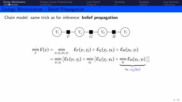
Submodular Energy Functions
I Binary variables: Yi = {0, 1} for all i ∈ VI Energy function: unary and pairwise factors
E (y ; x ,w) =∑i∈V
Ei (yi ) +∑
(i ,j)∈EEij(yi , yj)
Yi Yj
Xi Xj
I Restriction 1 (without loss of generality):
Ei (yi ) ≥ 0
(always achievable by adding a constant to E )
I Restriction 2 (submodularity):
Eij(yi , yj) = 0, if yi = yj ,
Eij(yi , yj) = Eij(yj , yi ) ≥ 0, otherwise.
”neighbors prefer to have the same labels”
13 / 40
Energy Minimization (Integer) Linear Programming Local Search Sampling Sampling Loss functions
Submodular Energy Functions
I Binary variables: Yi = {0, 1} for all i ∈ VI Energy function: unary and pairwise factors
E (y ; x ,w) =∑i∈V
Ei (yi ) +∑
(i ,j)∈EEij(yi , yj)
Yi Yj
Xi Xj
I Restriction 1 (without loss of generality):
Ei (yi ) ≥ 0
(always achievable by adding a constant to E )
I Restriction 2 (submodularity):
Eij(yi , yj) = 0, if yi = yj ,
Eij(yi , yj) = Eij(yj , yi ) ≥ 0, otherwise.
”neighbors prefer to have the same labels”13 / 40

Energy Minimization (Integer) Linear Programming Local Search Sampling Sampling Loss functions
Graph-Cuts Algorithm for Submodular Energy Minimization [Greig et al., 1989]
If conditions are fulfilled, energy minimization can be performed by a solving s-t-mincut:
I construct auxiliary undirected graph
I one node {i}i∈V per variable
I two extra nodes: source s, sink t
I weighted edges
Edge weight
{i , j} Eij(yi = 0, yj = 1){i , s} Ei (yi = 1){i , t} Ei (yi = 0)
I find s-t-cut of minimal weight(polynomial time using max-flow theorem)
i j k
l m n
s
t
{i, s}
{i, t}
From minimal weight cut we recover labeling of minimal energy:I y∗i = 1 if edge {i , s} is cut. Otherwise y∗i = 0
14 / 40

Energy Minimization (Integer) Linear Programming Local Search Sampling Sampling Loss functions
Integer Linear Programming (ILP)
General energy E (y) =∑
F EF (yF )
I variables with more than 2 states
I higher-order factors (more than 2 variables)
I non-submodular factors
Yi Yj
Yk Yl
Formulate as integer linear program (ILP)
I linear objective function
I linear constraints
I variables to optimize over are integer-valued
ILPs are in general NP-hard, but some individual instances can be solved
I standard optimization toolboxes: e.g. CPLEX, Gurobi, COIN-OR, . . .
15 / 40
Energy Minimization (Integer) Linear Programming Local Search Sampling Sampling Loss functions
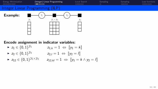
Integer Linear Programming (ILP)
Example:
Encode assignment in indicator variables:I z1 ∈ {0, 1}Y1 z1;k = 1 ⇔ Jy1 = kKI z2 ∈ {0, 1}Y2 z2;l = 1 ⇔ Jy2 = lKI z12 ∈ {0, 1}Y1×Y2 z12;kl = 1 ⇔ Jy1 = k ∧ y2 = lK
Consistency Constraints:∑k∈Y1
z1;k = 1,∑l∈Y2
z2;l = 1,∑
k,l∈Y1×Y2
z12;kl = 1 (indicator property)
∑k∈Y1
z12;kl = z2;l
∑l∈Y2
z12;kl = z1;k (consistency)
16 / 40

Energy Minimization (Integer) Linear Programming Local Search Sampling Sampling Loss functions
Integer Linear Programming (ILP)
Example: Y1 Y2
Y1 Y1 × Y2 Y2
y1 = 2
y2 = 3
(y1, y2) = (2, 3)
Encode assignment in indicator variables:I z1 ∈ {0, 1}Y1 , z2 ∈ {0, 1}Y2 , z12 ∈ {0, 1}Y1×Y2
Consistency Constraints:∑k∈Y1
z1;k = 1,∑l∈Y2
z2;l = 1,∑
k,l∈Y1×Y2
z12;kl = 1 (indicator property)
∑k∈Y1
z12;kl = z2;l
∑l∈Y2
z12;kl = z1;k (consistency)
16 / 40

Energy Minimization (Integer) Linear Programming Local Search Sampling Sampling Loss functions
Integer Linear Programming (ILP)
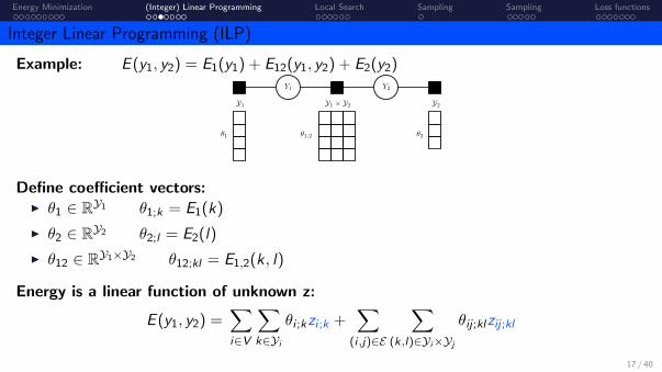
Example: E (y1, y2) = E1(y1) + E12(y1, y2) + E2(y2)Y1 Y2
Y1 Y1 × Y2 Y2
θ1 θ1,2 θ2
Define coefficient vectors:I θ1 ∈ RY1 θ1;k = E1(k)
I θ2 ∈ RY2 θ2;l = E2(l)
I θ12 ∈ RY1×Y2 θ12;kl = E1,2(k, l)
Energy is a linear function of unknown z:
E (y1, y2) =∑i∈V
∑k∈Yi
θi ;kJyi = kK +∑i ,j∈E
∑k,l∈Yi×Yj
θij ;klJyi = k ∧ yj = lK
17 / 40
Energy Minimization (Integer) Linear Programming Local Search Sampling Sampling Loss functions
Integer Linear Programming (ILP)
Example: E (y1, y2) = E1(y1) + E12(y1, y2) + E2(y2)Y1 Y2
Y1 Y1 × Y2 Y2
θ1 θ1,2 θ2
Define coefficient vectors:I θ1 ∈ RY1 θ1;k = E1(k)
I θ2 ∈ RY2 θ2;l = E2(l)
I θ12 ∈ RY1×Y2 θ12;kl = E1,2(k, l)
Energy is a linear function of unknown z:
E (y1, y2) =∑i∈V
∑k∈Yi
θi ;kzi ;k +∑
(i ,j)∈E
∑(k,l)∈Yi×Yj
θij ;klzij ;kl
17 / 40

Energy Minimization (Integer) Linear Programming Local Search Sampling Sampling Loss functions
Integer Linear Programming (ILP)
minz
∑i∈V
∑k∈Yi
θi ;kzi ;k +∑
(i ,j)∈E
∑(k,l)∈Yi×Yj
θij ;klzij ;kl
subject to zi ;k ∈ {0, 1} for all i ∈ V , ∀k ∈ Yi ,zij ;kl ∈ {0, 1} for all (i , j) ∈ E , (k, l) ∈ Yi × Yj ,∑k∈Yi
zi ;k = 1, for all i ∈ V ,
∑k,l∈Yi×Yj
zij ;kl = 1, for all (i , j) ∈ E ,
∑k∈Yi
zij ;kl = zj ;l for all (i , j) ∈ E , l ∈ Yj ,∑l∈Yj
zij ;kl = zi ;k for all (i , j) ∈ E , k ∈ Yi ,
NP-hard to solve because of integrality constraints.
18 / 40

Energy Minimization (Integer) Linear Programming Local Search Sampling Sampling Loss functions
Integer Linear Programming (ILP)
minz
∑i∈V
∑k∈Yi
θi ;kzi ;k +∑
(i ,j)∈E
∑(k,l)∈Yi×Yj
θij ;klzij ;kl
subject to zi ;k ∈ {0, 1} for all i ∈ V , ∀k ∈ Yi ,zij ;kl ∈ {0, 1} for all (i , j) ∈ E , (k, l) ∈ Yi × Yj ,∑k∈Yi
zi ;k = 1, for all i ∈ V ,
∑k,l∈Yi×Yj
zij ;kl = 1, for all (i , j) ∈ E ,
∑k∈Yi
zij ;kl = zj ;l for all (i , j) ∈ E , l ∈ Yj ,∑l∈Yj
zij ;kl = zi ;k for all (i , j) ∈ E , k ∈ Yi ,
NP-hard to solve because of integrality constraints. 18 / 40

Energy Minimization (Integer) Linear Programming Local Search Sampling Sampling Loss functions
Linear Programming (LP) Relaxation
minz
∑i∈V
∑k∈Yi
θi ;kzi ;k +∑
(i ,j)∈E
∑(k,l)∈Yi×Yj
θij ;klzij ;kl
subject to ((((((hhhhhhzi ;k ∈ {0, 1} zi ;k ∈ [0, 1] for all i ∈ V , ∀k ∈ Yi ,((((((hhhhhhzij ;kl ∈ {0, 1} zij ;kl ∈ [0, 1] for all (i , j) ∈ E , (k, l) ∈ Yi × Yj ,∑k∈Yi
zi ;k = 1, for all i ∈ V ,
∑k,l∈Yi×Yj
zij ;kl = 1, for all (i , j) ∈ E ,
∑k∈Yi
zij ;kl = zj ;l for all (i , j) ∈ E , l ∈ Yj ,∑l∈Yj
zij ;kl = zi ;k for all (i , j) ∈ E , k ∈ Yi ,
Relax constraints → optimization problem becomes tractable 19 / 40

Energy Minimization (Integer) Linear Programming Local Search Sampling Sampling Loss functions
Linear Programming (LP) Relaxation
Solution z∗LP might have fractional values
I → no corresponding labeling y ∈ YI → round LP solution to {0, 1} values
Problem:I rounded solution usually not optimal, i.e. not identical to ILP solution
LP relaxations perform approximate energy minimization20 / 40

Energy Minimization (Integer) Linear Programming Local Search Sampling Sampling Loss functions
Linear Programming (LP) Relaxation
Example: color quantization
Example: stereo reconstruction
Images: Berkeley Segmentation Dataset
21 / 40

Energy Minimization (Integer) Linear Programming Local Search Sampling Sampling Loss functions
Local Search
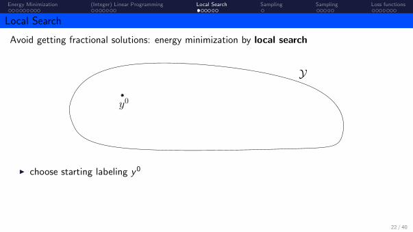
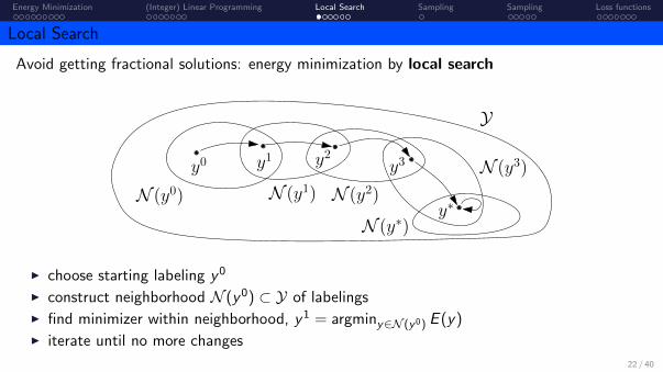
Avoid getting fractional solutions: energy minimization by local search
I choose starting labeling y0
I construct neighborhood N (y0) ⊂ Y of labelings
I find minimizer within neighborhood, y1 = argminy∈N (y0) E (y)
I iterate until no more changes
22 / 40
Energy Minimization (Integer) Linear Programming Local Search Sampling Sampling Loss functions
Local Search
Avoid getting fractional solutions: energy minimization by local search
y0
Y
I choose starting labeling y0
I construct neighborhood N (y0) ⊂ Y of labelingsI find minimizer within neighborhood, y1 = argminy∈N (y0) E (y)I iterate until no more changes
22 / 40

Energy Minimization (Integer) Linear Programming Local Search Sampling Sampling Loss functions
Local Search
Avoid getting fractional solutions: energy minimization by local search
y0
N (y0)
Y
I choose starting labeling y0
I construct neighborhood N (y0) ⊂ Y of labelings
I find minimizer within neighborhood, y1 = argminy∈N (y0) E (y)I iterate until no more changes
22 / 40

Energy Minimization (Integer) Linear Programming Local Search Sampling Sampling Loss functions
Local Search
Avoid getting fractional solutions: energy minimization by local search
y0 y1
N (y0)
Y
I choose starting labeling y0
I construct neighborhood N (y0) ⊂ Y of labelingsI find minimizer within neighborhood, y1 = argminy∈N (y0) E (y)
I iterate until no more changes
22 / 40
Energy Minimization (Integer) Linear Programming Local Search Sampling Sampling Loss functions
Local Search
Avoid getting fractional solutions: energy minimization by local search
y0 y1
N (y0) N (y1)
y2
N (y2)
y3
y∗
N (y3)
N (y∗)
Y
I choose starting labeling y0
I construct neighborhood N (y0) ⊂ Y of labelingsI find minimizer within neighborhood, y1 = argminy∈N (y0) E (y)I iterate until no more changes
22 / 40

Energy Minimization (Integer) Linear Programming Local Search Sampling Sampling Loss functions
Iterated Conditional Modes (ICM) [Besag, 1986]
Define local neighborhoods:I Ni (y) = {(y1, . . . , yi−1, y , yi+1, . . . , yn)|y ∈ Yi} for i ∈ V .
all labeling reachable from y by changing value of yi
. . .
ICM procedure:I neighborhood N (y) =
⋃i∈V Ni (y)
all states reachable from y by changing a single variable
I y t+1 = argminy∈N (y t)
E (y) by exhaustive search (∑
i |Yi | evaluations)
23 / 40

Energy Minimization (Integer) Linear Programming Local Search Sampling Sampling Loss functions
Iterated Conditional Modes (ICM) [Besag, 1986]
Define local neighborhoods:I Ni (y) = {(y1, . . . , yi−1, y , yi+1, . . . , yn)|y ∈ Yi} for i ∈ V .
all labeling reachable from y by changing value of yi
ICM procedure:I neighborhood N (y) =
⋃i∈V Ni (y)
all states reachable from y by changing a single variable
I y t+1 = argminy∈N (y t)
E (y) by exhaustive search (∑
i |Yi | evaluations)
Observation: larger neighborhood sizes are betterI ICM: |N (y)| linear in |V |→ many iterations to explore exponentially large Y
I ideal: |N (y)| exponential in |V |,→ but: we must ensure that argminy∈N (y) E (y) remains tractable
23 / 40

Energy Minimization (Integer) Linear Programming Local Search Sampling Sampling Loss functions
Multilabel Graph-Cut: α-expansion
I E (y) with unary and pairwise termsI Yi = L = {1, . . . ,K} for i ∈ V (multi-class)
Example: semantic segmentation
24 / 40

Energy Minimization (Integer) Linear Programming Local Search Sampling Sampling Loss functions
Multilabel Graph-Cut: α-expansion
I E (y) with unary and pairwise termsI Yi = L = {1, . . . ,K} for i ∈ V (multi-class)
Example: semantic segmentation
24 / 40

Energy Minimization (Integer) Linear Programming Local Search Sampling Sampling Loss functions
Multilabel Graph-Cut: α-expansion
I E (y) with unary and pairwise termsI Yi = L = {1, . . . ,K} for i ∈ V (multi-class)
Algorithm
I initialize y0 arbitrarily (e.g. everything label 0)I repeat
I for any α ∈ LI construct neighborhood:
N (y) ={
(y1, . . . , y|V |) : yi ∈ {yi , α}}
”each variable can keep its value or switch to α”I solve y ← argminy∈N (y) E (y)
I until y has not changed for a whole iteration
24 / 40

Energy Minimization (Integer) Linear Programming Local Search Sampling Sampling Loss functions
Multilabel Graph-Cut: α-expansion
Theorem [Boykov et al. 2001]
If all pairwise terms are metric, i.e. for all (i , j) ∈ E
Eij(k, l) ≥ 0 with Eij(k , l) = 0⇔ k = l
Eij(k, l) = Eij(l , k)
Eij(k, l) ≤ Eij(k,m) + Eij(m, l) for all k , l ,m
Then argminy∈N (y) E (y) can be solved optimally using GraphCut.
Theorem [Veksler 2001]. The solution, yα, returned by α-expansion fulfills
E (yα) ≤ 2c ·miny∈Y
E (y) for c = max(i ,j)∈E
maxk 6=l Eij(k , l)
mink 6=l Eij(k , l)
25 / 40

Energy Minimization (Integer) Linear Programming Local Search Sampling Sampling Loss functions
Example: Semantic Segmentation
E (y) =∑i∈V
Ei (yi ) + λ∑
(i ,j)∈EJyi 6= yjK ”Potts model”
I Eij(k, l) ≥ 0 Eij(k, l) = 0 ⇔ k = l Eij(k , l) = Eij(l , k) X
I Eij(k , l) ≤ Eij(k,m) + Eij(m, l) X
I c = max(i ,j)∈Emaxk 6=l Eij (k,l)mink 6=l Eij (k,l)
= 1
I factor-2 approximation guarantee: E (yα) ≤ 2 miny∈Y E (y)
26 / 40

Energy Minimization (Integer) Linear Programming Local Search Sampling Sampling Loss functions
Example: Stereo Estimation
E (y) =∑i∈V
Ei (yi ) + λ∑
(i ,j)∈E|yi − yj |
I |yi − yj | is metric X
I c = max(i ,j)∈Emaxk 6=l Eij (k,l)mink 6=l Eij (k,l)
= |L − 1|I weak guarantees, but often close to optimal labelings in practice
Images: Middlebury stereo vision dataset
27 / 40

Energy Minimization (Integer) Linear Programming Local Search Sampling Sampling Loss functions
Sampling
Sampling was a general purpose probabilistic inference method. Can we use it for prediction?
MAP prediction from samples:
I S = {x1, . . . , xN} samples from p(x)
I x∗ ← argmaxx∈S p(x)
I output x∗
Problem:
I will need many samples
I with x∗ = argmaxx∈X p(x): Pr(x∗ 6= x∗) = (1− p(x∗))N ≈ 1− Np(x∗)I for graphical model, probability values are tiny, e.g. p(x∗) = 10−100 can easily happen
I N ≈ 5 · 1099 required to have 50% chance28 / 40
Energy Minimization (Integer) Linear Programming Local Search Sampling Sampling Loss functions
Sampling
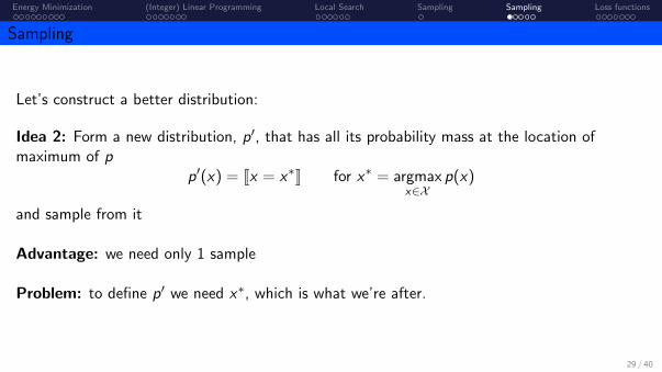
Let’s construct a better distribution:
Idea 2: Form a new distribution, p′, that has all its probability mass at the location ofmaximum of p
p′(x) = Jx = x∗K for x∗ = argmaxx∈X
p(x)
and sample from it
Advantage: we need only 1 sample
Problem: to define p′ we need x∗, which is what we’re after.
29 / 40

Energy Minimization (Integer) Linear Programming Local Search Sampling Sampling Loss functions
Sampling
Idea 3: do the same as idea 2, but more implicitly:
pβ(x) ∝ [p(x)]β for very large β
4 2 0 2 40.0
0.2
0.4
0.6
0.8
1.0
1.2
p(x)
4 2 0 2 40.0
0.2
0.4
0.6
0.8
1.0
1.2
[p(x)]2
4 2 0 2 40.0
0.2
0.4
0.6
0.8
1.0
1.2
[p(x)]10
4 2 0 2 40.0
0.2
0.4
0.6
0.8
1.0
1.2
[p(x)]100
Particularly easy for distributions in exponential form: p(x)∝e−E(x) becomes pβ(x)∝e−βE(x)
30 / 40

Energy Minimization (Integer) Linear Programming Local Search Sampling Sampling Loss functions
Simulated Annealing
Practical questions: How to choose β? How to sample from pβ?
These are often coupled, especially sampling works by a Monte Carlo Markov Chain (MCMC):I samples x1, x2, . . . from MCMC are dependent,I two consecutive samples are often similar to each other → random walk,I for a distribution with multiple peaks that are separated by a low-probability region,
MCMC sampling will jump around a peak, but very rarely switch peaks
4 2 0 2 40.0
0.2
0.4
0.6
0.8
1.0
1.2
p(x)
4 2 0 2 40.0
0.2
0.4
0.6
0.8
1.0
1.2
[p(x)]2
4 2 0 2 40.0
0.2
0.4
0.6
0.8
1.0
1.2
[p(x)]10
4 2 0 2 40.0
0.2
0.4
0.6
0.8
1.0
1.2
[p(x)]100
31 / 40

Energy Minimization (Integer) Linear Programming Local Search Sampling Sampling Loss functions
Sampling
Image: By Kingpin13 - Own work, CC0, https://commons.wikimedia.org/w/index.php?curid=2501076332 / 40

Energy Minimization (Integer) Linear Programming Local Search Sampling Sampling Loss functions
MAP Prediction / Energy Minimization – Summary
Task: compute argminy∈Y E (y |x)
Exact Energy Minimization
Only possible for certain models:
I trees/forests: max-sum belief propagation
I general graphs: junction chain algorithm (if tractable)
I submodular energies: GraphCut
I general graphs: integer linear programming (if tractable)
Approximate Energy Minimization
Many techniques with different properties and guarantees:
I linear programs relaxations, ICM, α-expansion
Best choices depends on model and requirements.33 / 40

Energy Minimization (Integer) Linear Programming Local Search Sampling Sampling Loss functions
Loss functions
34 / 40

Energy Minimization (Integer) Linear Programming Local Search Sampling Sampling Loss functions
Loss functions
We model structured data, e.g. y = (y1, . . . , ym). What makes a good prediction?
I The loss function is application dependent
∆ : Y × Y → R+,
35 / 40
Energy Minimization (Integer) Linear Programming Local Search Sampling Sampling Loss functions
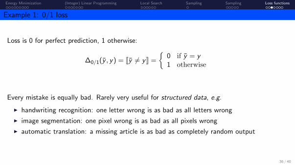
Example 1: 0/1 loss
Loss is 0 for perfect prediction, 1 otherwise:
∆0/1(y , y) = Jy 6= yK =
{0 if y = y1 otherwise
Every mistake is equally bad. Rarely very useful for structured data, e.g.
I handwriting recognition: one letter wrong is as bad as all letters wrong
I image segmentation: one pixel wrong is as bad as all pixels wrong
I automatic translation: a missing article is as bad as completely random output
36 / 40

Energy Minimization (Integer) Linear Programming Local Search Sampling Sampling Loss functions
Example 2: Hamming loss
Count the number of mislabeled variables:
∆H(y , y) =1
m
m∑i=1
Jym 6= ymK
x : I need a coffee break
y : subject verb article object object
y : subject verb article object verb
Jym 6= ymK 0 0 0 0 1
→ ∆H(y , y) = 0.2
Often used for graph labeling tasks, e.g. image segmentation, natural language processing, . . .
37 / 40

Energy Minimization (Integer) Linear Programming Local Search Sampling Sampling Loss functions
Example 3: Squared error
If the individual variables yi are numeric, e.g. pixel intensities,object locations, etc.
Sum of squared errors
∆Q(y , y) =1
m
m∑i=1
‖yi − yi‖2.
Used, e.g., in stereo reconstruction, optical flow estimation, . . .
38 / 40

Energy Minimization (Integer) Linear Programming Local Search Sampling Sampling Loss functions
Example 4: Task specific losses
Object detection
I bounding boxes, or
I arbitrarily shaped regionsground truth
detection
image
Intersection-over-union loss:
∆IoU(y , y) = 1− area(y ∩ y)
area(y ∪ y)= 1 −
Used, e.g., in PASCAL VOC challenges for object detection, because its scale-invariance.
39 / 40

Energy Minimization (Integer) Linear Programming Local Search Sampling Sampling Loss functions
Making Optimal Predictions
Given a structured distribution p(x , y) or p(y |x), what’s the best y to predict?
Decision theory: pick y∗ that causes minimal expected loss:
y∗ = argminy∈Y
Ey∼p(y |x){∆(y , y)} = argminy∈Y
∑y∈Y
∆(y , y)p(y |x)
For many loss functions not tractable to compute, but some exceptions:
I R∆0/1(y) = 1− p(y), so y∗ = argmaxy p(y) → use MAP prediction
I R∆H(y) = 1−∑i∈V p(yi ), so y∗ = (y∗1 , . . . , y
∗n ) with y∗i = argmax
k∈Yip(yi = k)
→ use marginal inference
40 / 40