Introduction to Practice of Molecular Simulation
333
Transcript of Introduction to Practice of Molecular Simulation


Introduction to Practice of Molecular Simulation

This page intentionally left blank

Introduction to Practice ofMolecular SimulationMolecular Dynamics, Monte Carlo,Brownian Dynamics,Lattice Boltzmann, DissipativeParticle Dynamics
Akira SatohAkita Prefectural University
Japan
AMSTERDAM � BOSTON � HEIDELBERG � LONDON � NEW YORK � OXFORD
PARIS � SAN DIEGO � SAN FRANCISCO � SINGAPORE � SYDNEY � TOKYO

Elsevier
32 Jamestown Road London NW1 7BY
30 Corporate Drive, Suite 400, Burlington, MA 01803, USA
First published 2011
Copyright r 2011 Elsevier Inc. All rights reserved
No part of this publication may be reproduced or transmitted in any form or by any means,
electronic or mechanical, including photocopying, recording, or any information storage
and retrieval system, without permission in writing from the publisher. Details on how to
seek permission, further information about the Publisher’s permissions policies and our
arrangement with organizations such as the Copyright Clearance Center and the Copyright
Licensing Agency, can be found at our website: www.elsevier.com/permissions
This book and the individual contributions contained in it are protected under copyright by
the Publisher (other than as may be noted herein).
Notices
Knowledge and best practice in this field are constantly changing. As new research and
experience broaden our understanding, changes in research methods, professional practices,
or medical treatment may become necessary.
Practitioners and researchers must always rely on their own experience and knowledge in
evaluating and using any information, methods, compounds, or experiments described
herein. In using such information or methods they should be mindful of their own safety and
the safety of others, including parties for whom they have a professional responsibility.
To the fullest extent of the law, neither the Publisher nor the authors, contributors, or editors,
assume any liability for any injury and/or damage to persons or property as a matter of
products liability, negligence or otherwise, or from any use or operation of any methods,
products, instructions, or ideas contained in the material herein.
British Library Cataloguing-in-Publication Data
A catalogue record for this book is available from the British Library
Library of Congress Cataloging-in-Publication Data
A catalog record for this book is available from the Library of Congress
ISBN: 978-0-12-385148-2
For information on all Elsevier publications
visit our website at www.elsevierdirect.com
This book has been manufactured using Print On Demand technology. Each copy is
produced to order and is limited to black ink. The online version of this book will show
color figures where appropriate.

Contents
Preface ix
1 Outline of Molecular Simulation and Microsimulation Methods 1
1.1 Molecular Dynamics Method 1
1.1.1 Spherical Particle Systems 2
1.1.2 Nonspherical Particle Systems 51.2 Monte Carlo Method 11
1.3 Brownian Dynamics Method 15
1.4 Dissipative Particle Dynamics Method 19
1.5 Lattice Boltzmann Method 24
2 Outline of Methodology of Simulations 29
2.1 Initial Positions 29
2.1.1 Spherical Particle Systems 29
2.1.2 Nonspherical Particle Systems 32
2.2 Initial Velocities 352.2.1 Spherical Particle Systems 35
2.2.2 Nonspherical Particle Systems 37
2.3 Reduction Methods of Computation Time 39
2.3.1 Cutoff Distance 39
2.3.2 Cell Index Method 41
2.3.3 Verlet Neighbor List Method 42
2.4 Boundary Conditions 43
2.4.1 Periodic Boundary Condition 432.4.2 Lees�Edwards Boundary Condition 45
3 Practice of Molecular Dynamics Simulations 493.1 Diffusion Phenomena in a System of Light and Heavy Molecules 49
3.1.1 Physical Phenomena of Interest 50
3.1.2 Specification of Problems in Equations 50
3.1.3 Verlet Algorithm 51
3.1.4 Parameters for Simulations 52
3.1.5 Results of Simulations 54
3.1.6 Simulation Program 55

3.2 Behavior of Rod-like Particles in a Simple Shear Flow 63
3.2.1 Physical Phenomena of Interest 643.2.2 Particle Model 64
3.2.3 Equation of Motion and Molecular Dynamics Algorithm 66
3.2.4 Modeling of Steric Repulsive Interaction 69
3.2.5 Nondimensionalization of Basic Equations 72
3.2.6 Treatment of the Criteria for Particle Overlap in Simulations 74
3.2.7 Parameters for Simulations 75
3.2.8 Results of Simulations 77
3.2.9 Simulation Program 81
4 Practice of Monte Carlo Simulations 1054.1 Orientational Phenomena of Rod-like Particles in an
Applied Magnetic Field 105
4.1.1 Physical Phenomena of Interest 105
4.1.2 Specification of Problems in Equations 106
4.1.3 Canonical Monte Carlo Algorithm 111
4.1.4 Parameters for Simulations 115
4.1.5 Results of Simulations 116
4.1.6 Simulation Program 1184.2 Aggregation Phenomena in a Dispersion of Plate-like Particles 134
4.2.1 Physical Phenomena of Interest 134
4.2.2 Particle Model 134
4.2.3 Criterion of the Particle Overlap 136
4.2.4 Canonical Monte Carlo Algorithm 143
4.2.5 Treatment of the Criterion of the Particle Overlap in
Simulations 143
4.2.6 Particle-Fixed Coordinate System and the Absolute
Coordinate System 144
4.2.7 Attempt of Small Angular Changes in the Particle
Axis and the Magnetic Moment 145
4.2.8 Parameters for Simulations 146
4.2.9 Results of Simulations 147
4.2.10 Simulation Program 150
5 Practice of Brownian Dynamics Simulations 173
5.1 Sedimentation Phenomena of Lennard-Jones Particles 173
5.2 Specification of Problems in Equations 173
5.3 Brownian Dynamics Algorithm 1745.4 Parameters for Simulations 176
5.5 Results of Simulations 176
5.6 Simulation Program 179
vi Contents

6 Practice of Dissipative Particle Dynamics Simulations 187
6.1 Aggregation Phenomena of Magnetic Particles 1876.2 Specification of Problems in Equations 187
6.2.1 Kinetic Equation of Dissipative Particles 187
6.2.2 Model of Particles 189
6.2.3 Model Potential for Interactions Between Dissipative
and Magnetic Particles 190
6.2.4 Nondimensionalization of the Equation of Motion
and Related Quantities 191
6.3 Parameters for Simulations 1936.4 Results of Simulations 194
6.5 Simulation Program 197
7 Practice of Lattice Boltzmann Simulations 219
7.1 Uniform Flow Around a Two-Dimensional Circular Cylinder 219
7.2 Specification of Problems in Equations 220
7.3 Boundary Conditions 221
7.4 Various Treatments in the Simulation Program 223
7.4.1 Definition and Evaluation of the Drag Coefficient 223
7.4.2 Choice of the Procedures by Coloring Lattice Sites 2247.4.3 Treatment of Interactions on the Cylinder Surface 225
7.4.4 Evaluation of the Velocity and Density 225
7.5 Nondimensionalization of the Basic Equations 226
7.6 Conditions for Simulations 227
7.6.1 Initial Distribution 227
7.6.2 Parameters for Simulations 227
7.7 Results of Simulations 227
7.8 Simulation Program 231
8 Theoretical Background of Lattice Boltzmann Method 255
8.1 Equilibrium Distribution 2558.1.1 D2Q9 Model 257
8.1.2 D3Q19 Model 264
8.2 Navier�Stokes Equation 271
8.3 Body Force 275
8.4 Boundary Conditions 277
8.4.1 Bounce-back Rule 277
8.4.2 BFL Method 279
8.4.3 YMLS Method 2818.4.4 Other Methods 282
8.5 Force and Torque Acting on Particles 282
8.6 Nondimensionalization 283
viiContents

Appendix 1: Chapman�Enskog Expansion 285
Appendix 2: Generation of Random Numbers According to GaussianDistribution 291
Appendix 3: Outline of Basic Grammars of FORTRAN and C Languages 293
Appendix 4: Unit Systems of Magnetic Materials 317
How to Acquire Simulation Programs 319
References 321
viii Contents

Preface
The control of internal structure during the fabrication of materials on the nano-
scale may enable us to develop a new generation of materials. A deeper under-
standing of phenomena on the microscopic scale may lead to completely new fields
of application. As a tool for microscopic analysis, molecular simulation methods—
such as the molecular dynamics and the Monte Carlo methods—have currently
been playing an extremely important role in numerous fields, ranging from pure
science and engineering to the medical, pharmaceutical, and agricultural sciences.
The importance of these methods is expected to increase significantly with the
advance of science and technology.
Many physics textbooks address the molecular simulation method for pure liquid
or solid systems. In contrast, textbooks concerning the simulation method for sus-
pensions or dispersions are less common; this fact provided the motivation for my
previous textbook. Moreover, students or nonexperts needing to apply the molecu-
lar simulation method to a physical problem have few tools for cultivating the skill
of developing a simulation program that do not require training under a supervisor
with expertise in simulation techniques. It became clear that students and nonexpert
researchers would find useful a textbook that taught the important concepts of the
simulation technique and honed programming skills by tackling practical physical
problems with guidance from sample simulation programs. This book would need
to be written carefully; it would not simply explain a sample simulation program,
but also explains the analysis procedures and include the essence of the theory, the
specification of the basic equations, the method of nondimensionalization, and
appropriate discussion of results. A brief explanation of the essence of the grammar
of programming languages also would be useful.
In order to apply the simulation methods to more complex systems, such as
carbon-nanotubes, polymeric liquids, and DNA/protein systems, the present book
addresses a range of practical methods, including molecular dynamics and Monte
Carlo, for simulations of practical systems such as the spherocylinder and the disk-
like particle suspension. Moreover, this book discusses the dissipative particle
dynamics method and the lattice Boltzmann method, both currently being devel-
oped as simulation techniques for taking into account the multibody hydrodynamic
interaction among dispersed particles in a particle suspension or among polymers
in a polymeric liquid.
The resulting characteristics of the present book are as follows. The important
and essential background relating to the theory of each simulation technique is
explained, avoiding complex mathematical manipulation as much as possible. The
equations that are included herein are all important expressions; an understanding

of them is key to reading a specialized textbook that treats the more theoretical
aspects of the simulation methods. Much of the methodology, such as the assign-
ment of the initial position and velocity of particles, is explained in detail in order
to be useful to the reader developing a practical simulation program.
In the chapters dedicated to advancing the reader’s practical skill for developing
a simulation program, the following methodology is adopted. First, the sample
physical phenomenon is described in order to discuss the simulation method that
will be addressed in the chapter. This is followed by a series of analyses (including
the theoretical backgrounds) that are conducted mainly from the viewpoint of
developing a simulation program. Then, the assignment of the important parameters
and the assumptions that are required for conducting the simulation of the physical
problem are described. Finally, results that have been obtained from the simulation
are shown and discussed, with emphasis on the visualization of the results by snap-
shots. Each example is conducted with a sample copy of the simulation program
from which the results were obtained, together with sufficient explanatory descrip-
tions of the important features in the simulation program to aid to the reader’s
understanding.
Most of the sample simulation programs are written in the FORTRAN language,
excepting the simulation program for the Brownian dynamics method. We take
into account that some readers may be unfamiliar with programming languages,
that is, the FORTRAN or the C language; therefore, an appendix explains the
important features of these programming languages from the viewpoint of develop-
ing a scientific simulation program. These explanations are expected to signifi-
cantly reduce the reader’s effort of understanding the grammar of the programming
languages when referring to a textbook of the FORTRAN or the C language.
The present book has been written in a self-learning mode as much as possible,
and therefore readers are expected to derive the important expressions for
themselves—that is the essence of each simulation demonstration. This approach
should appeal to the reader who is more interested in the theoretical aspects of the
simulation methods.
Finally, the author strongly hopes that this book will interest many students in
molecular and microsimulation methods and direct them to the growing number of
research fields in which these simulation methods are indispensable, and that one
day they will be the preeminent researchers in those fields.
The author deeply acknowledges contribution of Dr. Geoff N. Coverdale, who
volunteered valuable assistance during the development of the manuscript. The
author also wishes to express his thanks to Ms. Aya Saitoh for her dedication and
patience during the preparation of so many digital files derived from the handwrit-
ten manuscripts.
Akira Satoh
Kisarazu City, Chiba Prefecture, Japan
December 2010
x Preface

1 Outline of Molecular Simulationand Microsimulation Methods
In the modern nanotechnology age, microscopic analysis methods are indispensable
in order to generate new functional materials and investigate physical phenomena
on a molecular level. These methods treat the constituent species of a system, such
as molecules and fine particles. Macroscopic and microscopic quantities of interest
are derived from analyzing the behavior of these species.
These approaches, called “molecular simulation methods,” are represented by
the Monte Carlo (MC) and molecular dynamics (MD) methods [1�3]. MC methods
exhibit a powerful ability to analyze thermodynamic equilibrium, but are
unsuitable for investigating dynamic phenomena. MD methods are useful for ther-
modynamic equilibrium but are more advantageous for investigating the dynamic
properties of a system in a nonequilibrium situation. This book examines MD and
MC methods of a nonspherical particle dispersion in a three-dimensional system,
which may be directly applicable to such complicated dispersions as DNA and
polymeric liquids. This book also addresses Brownian dynamics (BD) methods
[1,4], which can simulate the Brownian motion of dispersed particles; dissipative
particle dynamics (DPD) [5�8]; and lattice Boltzmann methods [9�12], in which a
liquid system is regarded as composed of virtual fluid particles. Simulation meth-
ods using the concept of virtual fluid particles are generally used for pure liquid
systems, but are useful for simulating particle dispersions.
1.1 Molecular Dynamics Method
A spherical particle dispersion can be treated straightforwardly in simulations because
only the translational motion of particles is important, and the treatment of the rota-
tional motion is basically unnecessary. In contrast, since the translational and rota-
tional motion has to be simulated for an axisymmetric particle dispersion, MD
simulations become much more complicated in comparison with the spherical particle
system. Simulation techniques for a dispersion composed of nonspherical particles
with a general shape may be obtained by generalizing the methods employed to an
axisymmetric particle dispersion. It is, therefore, very important to understand the MD
method for the axisymmetric particle system.
Introduction to Practice of Molecular Simulation. DOI: 10.1016/B978-0-12-385148-2.00001-X
© 2011 Elsevier Inc. All rights reserved.

1.1.1 Spherical Particle Systems
The concept of the MD method is rather straightforward and logical. The motion of
molecules is generally governed by Newton’s equations of motion in classical the-
ory. In MD simulations, particle motion is simulated on a computer according to
the equations of motion. If one molecule moves solely on a classical mechanics
level, a computer is unnecessary because mathematical calculation with pencil and
paper is sufficient to solve the motion of the molecule. However, since molecules
in a real system are numerous and interact with each other, such mathematical anal-
ysis is impracticable. In this situation, therefore, computer simulations become a
powerful tool for a microscopic analysis.
If the mass of molecule i is denoted by mi, and the force acting on molecule i by
the ambient molecules and an external field denoted by fi, then the motion of a par-
ticle is described by Newton’s equation of motion:
mi
d2ri
dt25 f i ð1:1Þ
If a system is composed of N molecules, there are N sets of similar equations, and
the motion of N molecules interacts through forces acting among the molecules.
Differential equations such as Eq. (1.1) are unsuitable for solving the set of N
equations of motion on a computer. Computers readily solve simple equations, such
as algebraic ones, but are quite poor at intuitive solving procedures such as a trial-
and-error approach to find solutions. Hence, Eq. (1.1) will be transformed into an
algebraic equation. To do so, the second-order differential term in Eq. (1.1) must be
expressed as an algebraic expression, using the following Taylor series expansion:
xðt1 hÞ5 xðtÞ1 hdxðtÞdt
11
2!h2
d2xðtÞdt2
11
3!h3
d3xðtÞdt3
1? ð1:2Þ
Equation (1.2) implies that x at time (t1 h) can be expressed as the sum of x
itself, the first-order differential, the second-order differential, and so on, multiplied
by a constant for each term. If x does not significantly change with time, the higher-
order differential terms can be neglected for a sufficiently small value of the time
interval h. In order to approximate the second-order differential term in Eq. (1.1) as
an algebraic expression, another form of the Taylor series expansion is necessary:
xðt2 hÞ5 xðtÞ2 hdxðtÞdt
11
2!h2
d2xðtÞdt2
21
3!h3
d3xðtÞdt3
1? ð1:3Þ
If the first-order differential term is eliminated from Eqs. (1.2) and (1.3), the
second-order differential term can be solved as
d2xðtÞdt2
5xðt1 hÞ2 2xðtÞ1 xðt2 hÞ
h21Oðh2Þ ð1:4Þ
2 Introduction to Practice of Molecular Simulation

The last term on the right-hand side of this equation implies the accuracy of the
approximation, and, in this case, terms higher than h2 are neglected. If the second-
order differential is approximated as
d2xðtÞdt2
5xðt1 hÞ2 2xðtÞ1 xðt2 hÞ
h2ð1:5Þ
This expression is called the “central difference approximation.” With this approxi-
mation and the notation ri5 (xi, yi, zi) for the molecular position and fi5 (fxi, fyi,
fzi) for the force acting on particle i, the equation of the x-component of Newton’s
equation of motion can be written as
xiðt1 hÞ5 2xiðtÞ2 xiðt2 hÞ1 h2
mi
fxiðtÞ ð1:6Þ
Similar equations are satisfied for the other components. Since Eq. (1.6) is a
simple algebraic equation, the molecular position at the next time step can be
evaluated using the present and previous positions and the present force. If a
system is composed of N molecules, there are 3N algebraic equations for speci-
fying the motion of molecules; these numerous equations are solved on a com-
puter, where the motion of the molecules in a system can be pursued with the
time variable. Eq. (1.6) does not require the velocity terms for determining the
molecular position at the next time step. This scheme is called the “Verlet
method” [13]. The velocity, if required, can be evaluated from the central differ-
ence approximation as
viðtÞ5riðt1 hÞ2 riðt2 hÞ
2hð1:7Þ
This approximation can be derived by eliminating the second-order differential
terms in Eqs. (1.2) and (1.3). It has already been noted that the velocities are unnec-
essary for evaluating the position at the next time step; however, a scheme using the
positions and velocities simultaneously may be more desirable in order to keep the
system temperature constant. We show such a method in the following paragraphs.
If we take into account that the first- and second-order differentials of the posi-
tion are equal to the velocity and acceleration, respectively, the neglect of differen-
tial terms equal to or higher than third-order in Eq. (1.2) leads to the following
equation:
riðt1 hÞ5 riðtÞ1 hviðtÞ1h2
2mi
f iðtÞ ð1:8Þ
This equation determines the position of the molecules, but the velocity term
arises on the right-hand side, so that another equation is necessary for specifying
3Outline of Molecular Simulation and Microsimulation Methods

the velocity. The first-order differential of the velocity is equal to the
acceleration:
viðt1 hÞ5 viðtÞ1h
mi
f iðtÞ ð1:9Þ
In order to improve accuracy, the force term in Eq. (1.9) is slightly modified
and the following equation obtained:
viðt1 hÞ5 viðtÞ1h
2mi
ðf iðtÞ1 f iðt1 hÞÞ ð1:10Þ
The scheme of using Eqs. (1.8) and (1.10) for determining the motion of molecules
is called the “velocity Verlet method” [14]. It is well known that the velocity Verlet
method is significantly superior in regard to the stability and accuracy of a simulation.
Consider another representative scheme. Noting that the first-order differential
of the position is the velocity and that of the velocity is the acceleration, the appli-
cation of the central difference approximation to these first-order differentials leads
to the following equations:
riðt1 hÞ5 riðtÞ1 hviðt1 h=2Þ ð1:11Þ
viðt1 h=2Þ5 viðt2 h=2Þ1 h
mi
f iðtÞ ð1:12Þ
The scheme of pursuing the positions and velocities of the molecules with
Eqs. (1.11) and (1.12) is called the “leapfrog method” [15]. This name arises from
the evaluation of the positions and forces, and then the velocities, by using time
steps in a leapfrog manner. This method is also a significantly superior scheme in
regard to stability and accuracy, comparable to the velocity Verlet method.
The MD method is applicable to both equilibrium and nonequilibrium physical
phenomena, which makes it a powerful computational tool that can be used to simu-
late many physical phenomena (if computing power is sufficient).
We show the main procedure for conducting the MD simulation using the veloc-
ity Verlet method in the following steps:
1. Specify the initial position and velocity of all molecules.
2. Calculate the forces acting on molecules.
3. Evaluate the positions of all molecules at the next time step from Eq. (1.8).
4. Evaluate the velocities of all molecules at the next time step from Eq. (1.10).
5. Repeat the procedures from step 2.
In the above procedure, the positions and velocities will be evaluated at every
time interval h in the MD simulation. The method of specifying the initial positions
and velocities will be shown in Chapter 2.
Finally, we show the method of evaluating the system averages, which are
necessary to make a comparison with experimental or theoretical values. Since
4 Introduction to Practice of Molecular Simulation

microscopic quantities such as positions and velocities are evaluated at every time
interval in MD simulations, a quantity evaluated from such microscopic values—
for example, the pressure—will differ from that measured experimentally. In order
to compare with experimental data, instant pressure is sampled at each time step,
and these values are averaged during a short sampling time to yield a macroscopic
pressure. This average can be expressed as
A5XNn51
An=N ð1:13Þ
in which An is the nth sampled value of an arbitrary physical quantity A, and A,
called the “time average,” is the mathematical average of N sampling data.
1.1.2 Nonspherical Particle Systems
1.1.2.1 Case of Taking into Account the Inertia Terms
For the case of nonspherical particles, we need to consider the translational motion
of the center of mass of a particle and also the rotational motion about an axis
through the center of mass. Axisymmetric particles are very useful as a particle
model for simulations, so we will focus on the axisymmetric particle model in this
section. As shown in Figure 1.1, the important rotational motion is to be treated
about the short axis line. If the particle mass is denoted by m, the inertia moment
by I, the position and velocity vectors of the center of mass of particle i by ri and
vi, respectively, the angular velocity vector about the short axis by ωi, and the force
and torque acting on the particle by fi and Ti, respectively, then the equations of
motion concerning the translational and rotational motion can be written as
(A)
ωz
φzΔφz
e
x
y
z
(B)
(T )ω
Figure 1.1 Linear particle and angular velocity: (A) the axisymmetric particle and (B) the
coordinate system.
5Outline of Molecular Simulation and Microsimulation Methods

md2ri
dt25 f i ð1:14Þ
Idωi
dt5Ti ð1:15Þ
Since the translational velocity vi is related to the position vector ri as vi5 dri/dt,
we now consider the meaning of a quantity φi, which is related to the angular
velocity ωi as ωi5 dφi/dt. It is assumed that during a short time interval Δt, φi
changes into (φi1Δφi) where Δφi is expressed as Δφi5 (Δφix, Δφiy, Δφiz). Asshown in Figure 1.1B, ωz is related to the rotational angle in the xy-plane about the
z-axis, Δφz. The other components have the same meanings, so that φi and ωi for
particle i can be related in the following expression:
Δφi 5φiðt1ΔtÞ2φiðtÞ5ΔtωiðtÞ ð1:16Þ
Is the use of the quantity φi, corresponding to ri, general? It seems to be more
direct and more intuitive to use the unit vector ei denoting the particle direction
rather than the quantity φi. The change in ei during an infinitesimal time interval,
Δei, can be written using the angular velocity ωi as
ΔeiðtÞ5 eiðt1ΔtÞ2 eiðtÞ5ΔtωiðtÞ3 eiðtÞ ð1:17Þ
From Eqs. (1.16) and (1.17), ei can be related to φi as
ΔeiðtÞ5ΔφiðtÞ3 eiðtÞ ð1:18Þ
Equation (1.17) leads to the governing equation specifying the change of the parti-
cle direction:
deiðtÞdt
5ωiðtÞ3 eiðtÞ ð1:19Þ
Hence, Eq. (1.15) for the angular velocity and Eq. (1.19) for the particle direction
govern the rotational motion of an axisymmetric particle.
In order to solve Eqs. (1.15) and (1.19) for the rotational motion on a computer,
these equations have to be translated into finite difference equations. To do so, as
already explained, the first- and second-order differentials have to be expressed as
algebraic expressions using the finite difference approximations based on Taylor
series expansions. General finite difference expressions are as follows:
dxðtÞdt
5xðt1ΔtÞ2xðtÞ
Δt1OðΔtÞ; dxðtÞ
dt5
xðtÞ2 xðt2ΔtÞΔt
1OðΔtÞ
dxðtÞdt
5xðt1ΔtÞ2xðt2ΔtÞ
2Δt1OððΔtÞ2Þ
9>>>=>>>;
ð1:20Þ
6 Introduction to Practice of Molecular Simulation

d2xðtÞdt2
5xðt1ΔtÞ22xðtÞ1 xðt2ΔtÞ
ðΔtÞ2 1OððΔtÞ2Þ ð1:21Þ
The simplest algorithm can be obtained using the forward finite difference
approximation in Eq. (1.20) as
eiðt1ΔtÞ5 eiðtÞ1ΔtωiðtÞ3 eiðtÞωiðt1ΔtÞ5ωiðtÞ1Δt
TiðtÞI
9>=>; ð1:22Þ
This algorithm is quite straightforward and understandable, but in practice does not
have sufficient accuracy, since the error of the forward finite difference approxima-
tion is of the order of Δt. In order to improve the accuracy, the following algorithm
has already been presented.
If the new vector function ui(t) such as ui (t)5ωi (t)3 ei (t) is introduced,
Eq. (1.19) can be written as
deiðtÞdt
5 uiðtÞ ð1:23Þ
By conducting the operator 3 e from the right side on the both sides of Eq. (1.15),
the following equation is obtained:
dωiðtÞdt
3 eiðtÞ5 1
ITiðtÞ3 eiðtÞ ð1:24Þ
The left-hand side of this equation leads to
dωi
dt3 ei 5
dðωi 3 eiÞdt
2ωi 3dei
dt5
dui
dt2ωi 3 ui ð1:25Þ
By substituting this equation into Eq. (1.24), the following equation can be obtained:
duiðtÞdt
51
ITiðtÞ3 eiðtÞ1ωiðtÞ3 uiðtÞ5
1
ITiðtÞ3 eiðtÞ2 ωiðtÞ
�� ��2eiðtÞ5
1
ITiðtÞ3 eiðtÞ1λiðtÞeiðtÞ
ð1:26Þ
In the transformation from the first to the second expressions on the right-hand
side, we have used the identity a3 (b3 c)5 (a � c)b2 (a � b)c in evaluating
ω3 (ω3 e). The quantity λi (t) in the third expression has been introduced in order
to satisfy the following relationship:
eiUui 5 eiUðωi 3 eiÞ5 0 ð1:27Þ
7Outline of Molecular Simulation and Microsimulation Methods

We have now completed the transformation of the variables from ei and ωi to eiand ui for solving the rotational motion of particles.
According to the leapfrog algorithm [15], Eqs. (1.23) and (1.26) reduce to the
following algebraic equations:
eiðt1ΔtÞ5 eiðtÞ1Δtuiðt1Δt=2Þ ð1:28Þ
uiðt1Δt=2Þ5 uiðt2Δt=2Þ1ΔtTiðtÞ3 eiðtÞ
I1ΔtλiðtÞeiðtÞ ð1:29Þ
Another equation is necessary for determining the value of λi (t). The velocity
ui(t) can be evaluated from the arithmetic average of ui(t1Δt/2) and ui(t1Δt/2),
and the expression is finally written using Eq. (1.29) as
uiðtÞ 5uiðt1Δt=2Þ1 uiðt2Δt=2Þ
2
5 uiðt2Δt=2Þ1 Δt
2UTiðtÞ3 eiðtÞ
I1
Δt
2λiðtÞeiðtÞ
ð1:30Þ
Since ui(t) has to satisfy the orthogonality condition shown in Eq. (1.27), the sub-
stitution of Eq. (1.30) into Eq. (1.27) leads to the equation of λi(t) as
λiðtÞ5 22
ΔtUeiðtÞUuiðt2Δt=2Þ ð1:31Þ
In obtaining this expression, the identity a � (b3 a)5 0 has been used to evaluate
e � (T3 e).
Now all the equations have been derived for determining the rotational
motion of axisymmetric particles. With the value λi(t) in Eq. (1.31), ui at
(t1Δt/2) is first evaluated from Eq. (1.29), and then ei at (t1Δt) is obtained
from Eq. (1.28). This procedure shows that the solution of ui (t1Δt/2) gives
rise to the values of ei(t1Δt) and Ti(t1Δt), and these solutions lead to
ui(t1 3Δt/2), and so forth. This algorithm is therefore another example of a
leapfrog algorithm.
For the translational motion, the velocity Verlet algorithm may be used, and the
particle position ri(t1Δt) and velocity vi(t1Δt) can be evaluated as
riðt1ΔtÞ5 riðtÞ1ΔtviðtÞ1ðΔtÞ22m
f iðtÞ
viðt1ΔtÞ5 viðtÞ1Δt
2m
(f iðtÞ1 f iðt1ΔtÞ
)9>>>>=>>>>;
ð1:32Þ
8 Introduction to Practice of Molecular Simulation

These equations can be derived in a straightforward manner from the finite differ-
ence approximations in Eqs. (1.20) and (1.21).
We have shown all the equations for specifying the translational and rotational
motion of axisymmetric particles for the case of taking into account the inertia
terms. The main procedure for conducting the MD simulation is as follows:
1. Specify the initial configuration and velocity of the axisymmetric particles for the transla-
tional and rotational motion.
2. Calculate the forces and torques acting on particles.
3. Evaluate the positions and velocities of the translational motion at (t1Δt) from
Eq. (1.32).
4. Evaluate λi(t) (i5 1, 2, . . ., N) from Eq. (1.31).
5. Evaluate ui (i5 1, 2, . . ., N) at (t1Δt/2) from Eq. (1.29).
6. Evaluate the unit vectors ei ði5 1; 2; . . . ;NÞ at (t1Δt) from Eq. (1.28).
7. Advance one time step to repeat the procedures from step 2.
By following this procedure, the MD method for axisymmetric particles with
the inertia terms can simulate the positions and velocities, and the directions and
angular velocities, at every time interval Δt.
1.1.2.2 Case of Neglected Inertia Terms
When treating a colloidal dispersion or a polymeric solution, the Stokesian
dynamics and BD methods are usually employed as a microscopic or mesoscopic
analysis tool. In these methods, dispersed particles or polymers are modeled as
idealized spherical or dumbbell particles, but the base liquid is usually assumed
to be a continuum medium and its effect is included in the equations of motion
of the particles or the polymers only as friction terms. If particle size approxi-
mates to or is smaller than micron-order, the inertia terms may be considered as
negligible. In this section, we treat this type of small particles and neglect the
inertia terms. For the case of axisymmetric particles moving in a quiescent fluid,
the translational and angular velocities of particle i, vi and ωi, are written as
vi 51
η1
XAeiei 1
1
YAðI2 eieiÞ
� �UFi ð1:33Þ
ωi 51
η1
XCeiei 1
1
YCðI2 eieiÞ
� �UTi ð1:34Þ
in which XA, YA, XC, and YC are the resistance functions specifying the particle
shape. If the long- and short-axis lengths are denoted by 2a and 2b, respectively,
and the eccentricity is denoted by s (5(a22 b2)1/2/a), the resistance functions for
the spheroidal particle are written as [16�18]
XA 5 6πaU8
3U
s3
22s1 ð11 s2ÞL ; YA 5 6πaU16
3U
s3
2s1 ð3s2 2 1ÞL ð1:35Þ
9Outline of Molecular Simulation and Microsimulation Methods

XC 5 8πa3U4
3U
s3ð12 s2Þ2s2 ð12 s2ÞL ; YC 5 8πa3U
4
3U
s3ð22 s2Þ22s1 ð11 s2ÞL ð1:36Þ
in which L is a function of the eccentricity and is expressed as
L5 LðsÞ5 ln11 s
12 sð1:37Þ
For the case of s{1, Eqs. (1.35) and (1.36) are approximated using Taylor series
expansions as
XA 5 6πa�12
2
5s2 1?
�; YA 5 6πa
�12
3
10s2 1?
�ð1:38Þ
XC 5 8πa3�12
6
5s2 1?
�; YC 5 8πa3
�12
9
10s2 1?
�ð1:39Þ
In the limit of s-0, the well-known Stokes drag formula for a spherical particle
in a quiescent fluid can be obtained from Eqs. (1.33), (1.34), (1.38), and (1.39):
vi 51
6πηaFi; ωi 5
1
8πηa3Ti ð1:40Þ
It is possible to pursue the motion of an axisymmetric particle using Eqs. (1.33)
and (1.34), but further simplified equations can be used for the present axisymmet-
ric particle. For an axisymmetric particle, the translational motion can be decom-
posed into the motion in the long axis direction and that in a direction normal to
the particle axis. Similarly, the rotational motion can be decomposed into the rota-
tion about the particle axis and that about a line normal to the particle axis through
the mass center. If the force Fi acting on the particle is expressed as the sum of the
force Fjji parallel to the particle axis and the force Fi
\ normal to that axis, then
these forces can be expressed using the particle direction vector ei as
Fjji 5 eiðeiUFiÞ5 eieiUFi; F\
i 5Fi 2Fjji 5 ðI2 eieiÞUFi ð1:41Þ
With these expressions, the velocities vjji and vi\ parallel and normal to the particle
axis, respectively, can be written from Eq. (1.33) as
vjji 51
ηXAFjji ; v\i 5
1
ηYAF\i ð1:42Þ
10 Introduction to Practice of Molecular Simulation

Similarly, the angular velocities ωjji and ω\
i about the long and short axes, respec-
tively, are written from Eq. (1.34) as
ωjji 5
1
ηXCTjji ; ω\
i 51
ηYCT\i ð1:43Þ
According to Eqs. (1.42) and (1.43), vjji , v\i , ω
jji ; and ω\
i can be evaluated from
values of Fjji , F
\i , T
jji ; and T\
i . The translational velocity vi and angular velocity ωi
are then obtained as
vi 5 vjji 1 v\i ; ωi 5ωjji 1ω\
i ð1:44Þ
With the solutions of the translational and angular velocities at the time step t
shown in Eq. (1.44), the position vector ri and the particle direction vector ei at thenext time step (t1Δt) can finally be obtained as
riðt1ΔtÞ5 riðtÞ1ΔtviðtÞ ð1:45Þ
eiðt1ΔtÞ5 eiðtÞ1ΔtωiðtÞ3 eiðtÞ ð1:46Þ
Lastly, we show the main procedure for the simulation in the following steps:
1. Specify the initial configuration and velocity of all axisymmetric particles for the transla-
tional and rotational motion.
2. Calculate all the forces and torques acting on particles.
3. Evaluate Fjji ; F
\i ; T
jji ; and T\
i (i5 1, 2, . . ., N) from Eq. (1.41) and similar equations for
the torques.
4. Calculate vjji ; v\i ; ω
jji ; and ω\
i (i5 1, 2, . . ., N) from Eqs. (1.42) and (1.43).
5. Calculate vi and ωi (i5 1, 2, . . ., N) from Eq. (1.44).
6. Calculate ri and ei (i5 1, 2, . . ., N) at the next time step (t1Δt) from Eqs. (1.45) and
(1.46).
7. Advance one time step and repeat the procedures from step 2.
1.2 Monte Carlo Method
In the MD method, the motion of molecules (particles) is simulated according to
the equations of motion and therefore it is applicable to both thermodynamic equi-
librium and nonequilibrium phenomena. In contrast, the MC method generates a
series of microscopic states under a certain stochastic law, irrespective of the equa-
tions of motion of particles. Since the MC method does not use the equations of
motion, it cannot include the concept of explicit time, and thus is only a simulation
technique for phenomena in thermodynamic equilibrium. Hence, it is unsuitable for
the MC method to deal with the dynamic properties of a system, which are depen-
dent on time. In the following paragraphs, we explain important points of the con-
cept of the MC method.
11Outline of Molecular Simulation and Microsimulation Methods

How do microscopic states arise for thermodynamic equilibrium in a practical
situation? We discuss this problem by considering a two-particle attractive system
using Figure 1.2. As shown in Figure 1.2A, if the two particles overlap, then a
repulsive force or a significant interaction energy arises. As shown in Figure 1.2B,
for the case of close proximity, the interaction energy becomes low and an attrac-
tive force acts on the particles. If the two particles are sufficiently distant, as shown
in Figure 1.2C, the interactive force is negligible and the interaction energy can be
regarded as zero. In actual phenomena, microscopic states which induce a signifi-
cantly high energy, as shown in Figure 1.2A, seldom appear, but microscopic states
which give rise to a low-energy system, as shown in Figure 1.2B, frequently arise.
However, this does not mean that only microscopic states that induce a minimum-
energy system appear. Consider the fact that oxygen and nitrogen molecules do not
gather in a limited area, but distribute uniformly in a room. It is seen from this dis-
cussion that, for thermodynamic equilibrium, microscopic states do not give rise to
a minimum of the total system energy, but to a minimum free energy of a system.
For example, in the case of a system specified by the number of particles N, tem-
perature T, and volume of the system V, microscopic states arise such that the fol-
lowing Helmholtz free energy F becomes a minimum:
F5E2 TS ð1:47Þ
in which E is the potential energy of the system, and S is the entropy. In the pre-
ceding example, the reason why oxygen or nitrogen molecules do not gather in a
limited area can be explained by taking into account the entropy term on the
right-hand side in Eq. (1.47). That is, the situation in which molecules do not
gather together and form flocks but expand to fill a room gives rise to a large
value of the entropy. Hence, according to the counterbalance relationship of the
energy and the entropy, real microscopic states arise such that the free energy of a
system is at minimum.
Next, we consider how microscopic states arise stochastically. We here treat a
system composed of N interacting spherical particles with temperature T and vol-
ume V of the system; these quantities are given values and assumed to be constant.
If the position vector of an arbitrary particle i (i5 1, 2, . . ., N) is denoted by ri,
then the total interaction energy U of the system can be expressed as a function of
the particle positions; that is, it can be expressed as U5U(r1, r2,. . .,rN). For thepresent system specified by given values of N, T, and V, the appearance of a
microscopic state that the particle i (i5 1, 2, . . ., N) exits within the small range
(A) Overlapping (B) Close proximity (C) Sufficiently distant
Figure 1.2 Typical energy situations for a two particle system.
12 Introduction to Practice of Molecular Simulation

of ri B (ri1Δri) is governed by the probability density function ρ(r1, r2,. . .,rN).This can be expressed from statistical mechanics [19,20] as
ρðr1; r2; . . . ; rNÞ5expf2Uðr1; r2; . . . ; rNÞ=kTgÐ
V. . .ÐVexpf2Uðr1; r2; . . . ; rNÞ=kTgdr1 dr2 . . . drN
ð1:48Þ
If a series of microscopic states is generated with an occurrence according to
this probability, a simulation may have physical meaning. However, this approach
is impracticable, as it is extraordinarily difficult and almost impossible to evaluate
analytically the definite integral of the denominator in Eq. (1.48). In fact, if we
were able to evaluate this integral term analytically, we would not need a computer
simulation because it would be possible to evaluate almost all physical quantities
analytically.
The “Metropolis method” [21] overcomes this difficulty for MC simulations. In
the Metropolis method, the transition probability from microscopic states i to j, pij,
is expressed as
pij 5
1 ðfor ρj=ρi $ 1Þρjρi
ðfor ρj=ρi , 1Þ
8<: ð1:49Þ
in which ρj and ρi are the probability density functions for microscopic states j and
i appearing, respectively. The ratio of ρj/ρi is obtained from Eq. (1.48) as
ρjρi
5 exp 21
kTðUj 2UiÞ
8<:
9=;
5 exp 21
kTUðr1j; r2j; . . . ; rNjÞ2Uðr1i; r2i; . . . ; rNiÞ� �2
435
ð1:50Þ
In the above equations, Ui and Uj are the interaction energies of microscopic
states i and j, respectively. The superscripts attached to the position vectors denote
the same meanings concerning microscopic states. Eq. (1.49) implies that, in the
transition from microscopic states i to j, new microscopic state j is adopted if the
system energy decreases, with the probability ρj/ρi (,1) if the energy increases. As
clearly demonstrated by Eq. (1.50), for ρj/ρi the denominator in Eq. (1.48) is not
required in Eq. (1.50), because ρj is divided by ρi and the term is canceled through
this operation. This is the main reason for the great success of the Metropolis
method for MC simulations. That a new microscopic state is adopted with the prob-
ability ρj/ρi, even in the case of the increase in the interaction energy, verifies the
accomplishment of the minimum free-energy condition for the system. In other
words, the adoption of microscopic states, yielding an increase in the system
energy, corresponds to an increase in the entropy.
13Outline of Molecular Simulation and Microsimulation Methods

The above discussion is directly applicable to a system composed of nonspheri-
cal particles. The situation of nonspherical particles in thermodynamic equilibrium
can be specified by the particle position of the mass center, ri(i5 1, 2, . . ., N), andthe unit vector ei(i5 1, 2, . . ., N) denoting the particle direction. The transition
probability from microscopic states i to j, pij can be written in similar form to
Eq. (1.49). The exact expression of ρj/ρi becomes
ρjρi
5 exp 21
kTðUj2UiÞ
8<:
9=;5exp 2
1
kT
(Uðr j
1 ; rj2 ; r
jN ; e
j1 ; e
j2 ; . . . ; e
jNÞ
24
2Uðr j1 ; r
j2 ; r
jN ; e
j1 ; e
j2 ; . . . ; e
jN�#
ð1:51Þ
The main procedure for the MC simulation of a nonspherical particle system is
as follows:
1. Specify the initial position and direction of all particles.
2. Regard this state as microscopic state i, and calculate the interaction energy Ui.
3. Choose an arbitrary particle in order or randomly and call this particle “particle α.”4. Make particle α move translationally using random numbers and calculate the interaction
energy Uj for this new configuration.
5. Adopt this new microscopic state for the case of Uj#Ui and go to step 7.
6. Calculate ρj/ρi in Eq. (1.51) for the case of Uj.Ui and take a random number R1 from a
uniform random number sequence distributed from zero to unity.
6.1. If R1# ρj/ρi, adopt this microscopic state j and go to step 7.
6.2. If R1. ρj/ρi, reject this microscopic state, regard previous state i as new microscopic
state j, and go to step 7.
7. Change the direction of particle α using random numbers and calculate the interaction
energy Uk for this new state.
8. If Uk#Uj, adopt this new microscopic state and repeat from step 2.
9. If Uk.Uj, calculate ρk/ρj in Eq. (1.51) and take a random number R2 from the uniform
random number sequence.
9.1. If R2# ρk/ρj, adopt this new microscopic state k and repeat from step 2.
9.2. If R2. ρk/ρj, reject this new state, regard previous state j as new microscopic state k,
and repeat from step 2.
Although the treatment of the translational and rotational changes is carried out
separately in the above algorithm, a simultaneous procedure is also possible in
such a way that the position and direction of an arbitrary particle are simulta-
neously changed, and the new microscopic state is adopted according to the condi-
tion in Eq. (1.49). However, for a strongly interacting system, the separate
treatment may be found to be more effective in many cases.
We will now briefly explain how the translational move is made using ran-
dom numbers during a simulation. If the position vector of an arbitrary particle
α in microscopic state i is denoted by rα5 (xα, yα, zα), this particle is moved
to a new position rα0 5 (xα
0 , yα0 , zα
0 ) by the following equations using random
14 Introduction to Practice of Molecular Simulation

numbers R1, R2, and R3, taken from a random number sequence ranged from
zero to unity:
xα0 5 xα 1R1δrmax
yα0 5 yα 1R2δrmax
zα0 5 zα 1R3δrmax
9=; ð1:52Þ
These equations imply that the particle is moved to an arbitrary position, deter-
mined by random numbers, within a cube centered at the particle center with side
length of 2δrmax. A series of microscopic states is generated by moving the parti-
cles according to the above-mentioned procedure.
Finally, we show the method of evaluating the average of a physical quantity in
MC simulations. These averages, called “ensemble averages,” are different from
the time averages that are obtained from MD simulations. If a physical quantity A
is a function of the microscopic states of a system, and An is the nth sampled value
of this quantity in an MC simulation, then the ensemble average hAi can be evalu-
ated from the equation
hAi5XMn51
An=M ð1:53Þ
in which M is the total sampling number. In actual simulations, the sampling proce-
dure is not conducted at each time step but at regular intervals. This may be more
efficient because if the data have significant correlations they are less likely to be
sampled by taking a longer interval for the sampling time. The ensemble averages
obtained in this way may be compared with experimental data.
1.3 Brownian Dynamics Method
A dispersion or suspension composed of fine particles dispersed in a base liquid is a
difficult case to be treated by simulations in terms of the MD method, because the
characteristic time of the motion of the solvent molecules is considerably different
from that of the dispersed particles. Simply speaking, if we observe such a disper-
sion based on the characteristic time of the solvent molecules, we can see only
the active motion of solvent molecules around the quiescent dispersed particles.
Clearly the MD method is quite unrealistic as a simulation technique for particle
dispersions. One approach to overcome this difficulty is to not focus on the motion
of each solvent molecule, but regard the solvent molecules as a continuum medium
and consider the motion of dispersed particles in such a medium. In this approach,
the influence of the solvent molecules is included into the equations of motion of
the particles as random forces. We can observe such random motion when pollen
moves at a liquid surface or when dispersed particles move in a functional fluid such
as a ferrofluid. The BD method simulates the random motion of dispersed particles
15Outline of Molecular Simulation and Microsimulation Methods

that is induced by the solvent molecules; thus, such particles are called “Brownian
particles.”
If a particle dispersion is so significantly dilute that each particle can be
regarded as moving independently, the motion of this Brownian particle is gov-
erned by the following Langevin equation [22]:
mdv
dt5 f2 ξv1 fB ð1:54Þ
This equation is valid for a spherical particle dispersion. In Eq. (1.54), m is the
mass of a spherical particle, v is the velocity vector, ξ is the friction coefficient and
is expressed as ξ5 3πηd for the particle diameter d with the viscosity η of a base
liquid, f is the force exerted by an external field, and fB (5( fxB, fy
B, fzB)) is the ran-
dom force due to the motion of solvent molecules. This random force has the fol-
lowing stochastic properties:
f Bx ðtÞ
5 f By ðtÞD E
5 f Bz ðtÞ
5 0 ð1:55Þ
f Bx ðtÞ� �2D E
5 f By ðtÞn o2� �
5 f Bz ðtÞ� �2D E
5 2ξkTδðt2 t0Þ ð1:56Þ
in which δ(t2 t0) is the Dirac delta function. In Eq. (1.56) larger random forces act
on Brownian particles at a higher temperature because the mean square average of
each component of the random force is in proportion to the system temperature. At
a higher temperature the solvent molecules move more actively and induce larger
random forces.
In order to simulate the Brownian motion of particles, the basic equation in
Eq. (1.54) has to be transformed into an algebraic equation, as in the MD method.
If the time interval h is sufficiently short such that the change in the forces is negli-
gible, Eq. (1.54) can be regarded as a simple first-order differential equation.
Hence, Eq. (1.54) can be solved by standard textbook methods of differential equa-
tions [23], and algebraic equations can finally be obtained as
rðt1 hÞ5 rðtÞ1 m
ξvðtÞ 12 exp 2
ξmh
� �� �
11
ξfðtÞ h2
m
ξ12 exp 2
ξmh
� �� �� �1ΔrB
ð1:57Þ
vðt1 hÞ5 vðtÞexp 2ξmh
� �1
1
ξfðtÞ 12 exp 2
ξmh
� �� �1ΔvB ð1:58Þ
in which ΔrB and ΔvB are a random displacement and velocity due to the motion
of solvent molecules. The relationship of the x-components of ΔrB and ΔvB can
16 Introduction to Practice of Molecular Simulation

be expressed as a two-dimensional normal distribution (similarly for the other com-
ponents). We do not show such an expression here [4], but instead consider a
method that is superior in regard to the extension of the BD method to the case
with multibody hydrodynamic interactions. The BD method based on Eqs. (1.57)
and (1.58) is applicable to physical phenomena in which the inertia term is a gov-
erning factor.
Since the BD method with multibody hydrodynamic interactions among the par-
ticles is very complicated, we here focus on an alternative method that treats the
friction forces between the particles and a base liquid, and the nonhydrodynamic
interactions between the particles. This simpler type of simulation method is some-
times used as a first-order approximation because of the complexity of treating
hydrodynamic interactions. A representative nonhydrodynamic force is the mag-
netic force influencing the magnetic particles in a ferrofluid.
Although the BD method based on the Ermak�McCammon analysis [24] takes
into account multibody hydrodynamic interactions among particles, we apply this
analysis method to the present dilute dispersion without hydrodynamic interactions,
and can derive the basic equation of the position vector ri(i5 1, 2,. . ., N) of
Brownian particle i as
riðt1 hÞ5 riðtÞ11
ξhf iðtÞ1ΔrBi ð1:59Þ
in which the components (ΔxBi ;ΔyBi ;ΔzBi ) of the random displacement ΔrBi have
to satisfy the following stochastic properties:
ΔxBi
5 ΔyBi
5 ΔzBi
5 0 ð1:60Þ
ΔxBi �2D E
5 ΔyBi �2D E
5 ΔzBi �2D E
52kT
ξh ð1:61Þ
Equations similar to Eq. (1.59) hold for every particle in the system. Interactions
among particles arise through the force fi(i5 1, 2,. . ., N) acting on them.
If a Brownian particle exhibits magnetic properties and has, for example, a mag-
netic dipole moment at the particle center, it will have a tendency to incline in the
direction of an applied magnetic field. Hence, even in the case of spherical parti-
cles, the rotational motion is influenced by an external field, so that both the trans-
lational and the rotational motion of a particle are treated simultaneously in
simulations.
If the unit vector of the particle direction is denoted by ni, the equation of the
change in ni can be derived under the same conditions assumed in deriving
Eq. (1.59) as
niðt1 hÞ5 niðtÞ11
ξRhTiðtÞ3 niðtÞ1ΔnBi ð1:62Þ
17Outline of Molecular Simulation and Microsimulation Methods

in which ξR is the friction coefficient of the rotational motion, expressed as
ξR5πηd3, and Ti is the torque acting on particle i by nonhydrodynamic forces.
Also, ΔnBi is the rotational displacement due to random forces, expressed as
ΔnBi 5ΔφB\1n\1 1ΔφB
\2n\2 ð1:63Þ
in which n\1 and n\2 are a set of unit vectors normal to the direction of particle i,
and ΔφB\1 and ΔφB
\2 have the following stochastic properties:
ΔφB\1
5 ΔφB
\2
5 0 ð1:64Þ
ΔφB\1
�2D E5 ΔφB
\2
�2D E5
2kT
ξRh ð1:65Þ
Now consider the correspondence of quantities in the translational and rotational
motion. The velocity vi in the translational motion corresponds to the angular
velocity ωi in the rotational motion, and the position vector ri corresponds to the
quantity φi defined as dφi/dt5ωi. Obviously, due to the similarity of Eqs. (1.64)
and (1.65) to Eqs. (1.60) and (1.61), the components ΔφB\1 and ΔφB
\2 of the vector
ΔφB have to satisfy Eqs. (1.64) and (1.65).
The basic Eqs. (1.59) and (1.62) for governing the translational and rotational
motion of particles have been derived under the assumptions that the momentum of
particles is sufficiently relaxed during the time interval h and that the force acting on
the particles is substantially constant during this infinitesimally short time. This is
the essence of the Ermak�McCammon method for BD simulations.
Next, we show the method of generating random displacements according to
Eqs. (1.60) and (1.61), but, before that, the normal probability distribution needs to
be briefly described. If the behavior of a stochastic variable is described by the nor-
mal distribution ρnormal(x) with variance σ2, ρnormal(x) is written as
ρnormalðxÞ51
ð2πσ2Þ1=2expð2 x2=2σ2Þ ð1:66Þ
in which the variance σ2 is a measure of how wide the stochastic variable x is dis-
tributed around the mean value hxi, which is taken as zero for this discussion. The
variance σ2 is mathematically defined as
σ2 5 hðx2 hxiÞ2i5 hx2i2 ðhxiÞ2 ð1:67Þ
If Eq. (1.66) is applied to Eqs. (1.60) and (1.61), the random displacement ΔxBiin the x-direction can be written in normal distribution form as
ρnormalðΔxBi Þ5ξ
4πkTh
� �1=2
exp 2ξ
4kThΔxBi �2� �
ð1:68Þ
18 Introduction to Practice of Molecular Simulation

The other components also obey a normal distribution. As seen in Eq. (1.68),
larger random displacements tend to arise at a higher system temperature, which
makes sense given that solvent molecules move more actively in the higher temper-
ature case. The random displacements can therefore be generated by sampling
according to the normal distributions shown in Eq. (1.68). An example of generat-
ing random displacements is shown in Appendix A2.
The main procedure for conducting the BD simulation based on Eqs. (1.59),
(1.60), and (1.61) is:
1. Specify the initial position of all particles.
2. Calculate the forces acting on each particle.
3. Generate the random displacements ΔrBi 5 (ΔxBi , ΔyBi , ΔzBi ) (i5 1, 2,. . ., N) using
uniform random numbers: for example, ΔxBi is sampled according to Eq. (1.68).
4. Calculate all the particle positions at the next time step from Eq. (1.59).
5. Return to step 2 and repeat.
The physical quantities of interest are evaluated by the time average, similar to
the molecular dynamics method.
1.4 Dissipative Particle Dynamics Method
As already pointed out, it is not realistic to use the MD method to simulate the
motion of solvent molecules and dispersed particles simultaneously, since the char-
acteristic time of solvent molecules is much shorter than that of dispersed particles.
Hence, in the BD method, the motion of solvent molecules is not treated, but a fluid
is regarded as a continuum medium. The influence of the molecular motion is com-
bined into the equations of motion of dispersed particles as stochastic random forces.
Are there any simulation methods to simulate the motion of both the solvent mole-
cules and the dispersed particles? As far as we treat the motion of real solvent mole-
cules, the development of such simulation methods may be impractical. However, if
groups or clusters of solvent molecules are regarded as virtual fluid particles, such
that the characteristic time of the motion of such fluid particles is not so different
from that of dispersed particles, then it is possible to simulate the motion of the dis-
persed and the fluid particles simultaneously. These virtual fluid particles are
expected to exchange their momentum, exhibit a random motion similar to
Brownian particles, and interact with each other by particle�particle potentials. We
call these virtual fluid particles “dissipative particles,” and the simulation technique
of treating the motion of dissipative particles instead of the solvent molecules is
called the “dissipative particle dynamics (DPD) method” [4�8].
The DPD method is principally applicable to simulations of colloidal dispersions
that take into account the multibody hydrodynamic interactions among particles.
For colloidal dispersions, the combination of the flow field solutions for a three- or
four-particle system into a simulation technique enables us to address the physical
situation of multibody hydrodynamic interactions as accurately as possible.
However, it is extraordinarily difficult to solve analytically the flow field even for
19Outline of Molecular Simulation and Microsimulation Methods

a three-particle system, so a solution for a nonspherical particle system is futile to
attempt. In contrast, the DPD method does not require this type of solution of the
flow field in conducting simulations of colloidal dispersions that take into account
multibody hydrodynamic effects. This is because they are automatically reproduced
from consideration of the interactions between the dissipative and the colloidal par-
ticles. This approach to the hydrodynamic interactions is a great advantage of the
DPD method. In addition, this method is applicable to nonspherical particle disper-
sions, and a good simulation technique for colloidal dispersions.
We will show the general categories of models employed in the modeling of a
fluid for numerical simulations before proceeding to the explanation of the DPD
method. Figure 1.3 schematically shows the classification of the modeling of a fluid.
Figure 1.3A shows a continuum medium model for a fluid. In this case, a solution of
a flow field can be obtained by solving the Navier�Stokes equations, which are the
governing equations of the motion of a fluid. Figure 1.3C shows a microscopic
model in which the solvent molecules are treated and a solution of the flow field can
be obtained by pursuing the motion of the solvent molecules: this is the MD
approach. Figure 1.3B shows a mesoscopic model in which a fluid is assumed to be
composed of virtual fluid particles: the DPD method is classified within this
category.
In the following paragraphs, we discuss the equations of motion of the dissipa-
tive particles for a system composed of dissipative particles alone, without colloidal
Figure 1.3 Modeling of a fluid: (A) the macroscopic model, (B) the mesoscopic model, and
(C) the microscopic model.
20 Introduction to Practice of Molecular Simulation

particles. For simplification’s sake, dissipative particles are simply called “parti-
cles” unless specifically identified.
In order that the solution of a flow field obtained from the particle motion
agrees with that of the Navier�Stokes equations, the equations of motion of the
particles have to be formalized in physically viable form. For example, as a physi-
cal restriction on the system behavior, the total momentum of a system should be
conserved. The forces acting on particle i possibly seem to be a conservative force
FijC, exerted by other particles (particle j in this case); a dissipative force Fij
D, due to
the exchange of momentum; and a random force FijR, inducing the random motion
of particles. With the particle mass m and the particle velocity vi, the equation of
motion can be written as
mdvi
dt5Xjð6¼iÞ
FCij 1
Xjð6¼iÞ
FDij 1
Xjð6¼iÞ
FRij ð1:69Þ
The subscripts in Eq. (1.69), for example in FijC, represent the force acting on
particle i by particle j. Now, we embody specific expressions for each force. Since
FijC is a conservative force between particles i and j, it is assumed to be dependent
on the relative position rij (5ri2 rj) alone, not on velocities. This specific expres-
sion will be shown later. FijD and Fij
R have to be conserved under a Galilean trans-
formation (refer to a textbook of mechanics); thus, they must be independent of riand vi in a given reference frame (quantities dependent on ri and vi are not con-
served), but should be functions of the relative position vector rij and relative
velocity vector vij (5vi2 vj). Furthermore, it is physically reasonable to assume
that FijR is dependent only on the relative position rij, and not on the relative veloc-
ity vij. We also have to take into account that the particle motion is isotropic and
the forces between particles decrease with the particle�particle separation. The
following expressions for FijD and Fij
R satisfy all the above-mentioned requirements:
FDij 5 2γwDðrijÞðeijUvijÞeij ð1:70Þ
FRij 5σwRðrijÞeijζ ij ð1:71Þ
in which rij5 jrijj, and eij is the unit vector denoting the direction of a line drawn
from particles j to i, expressed as eij5 rij/rij. The ζ ij is the stochastic variable induc-ing the random motion of particles and has the following characteristics:
hζ iji5 0; hζ ijðtÞζ i0j0 ðt0Þi5 ðδii0δjj0 1 δij0δji0 Þδðt2 t0Þ ð1:72Þ
in which δij is the Kronecker delta, and δij5 1 for i5 j and δij5 0 for the other
cases. Since this variable satisfies the equation of ζ ij5 ζ ji, the total momentum of a
system is conserved. The wD(rij) and wR(rij) are weighting functions representing
the characteristics of forces decreasing with the particle�particle separation, and γand σ are constants specifying the strengths of the corresponding forces. As shown
21Outline of Molecular Simulation and Microsimulation Methods

later, these constants are related to the system temperature and friction coefficients.
The FijD acts such that the relative motion of particles i and j relaxes, and Fij
R func-
tions such that the thermal motion is activated. Since the action�reaction law is
satisfied by FijR, the conservation of the total momentum is not violated by Fij
R.
By substituting Eqs. (1.70) and (1.71) into Eq. (1.69), the equation of motion of
particles can be written as
mdvi
dt5Xjð6¼iÞ
FCij ðrijÞ2
Xjð6¼iÞ
γwDðrijÞðeijUvijÞeij 1Xjð6¼iÞ
σwRðrijÞeijζ ij ð1:73Þ
The integral of this equation with respect to the time from t to (t1Δt) leads to
the finite difference equations specifying the motion of the simulation particles:
Δri 5 viΔt ð1:74Þ
Δvi 51
m
Xjð6¼iÞ
FCij ðrijÞ2
Xjð6¼iÞ
γwDðrijÞðeijUvijÞeij !
Δt11
m
Xjð6¼iÞ
σwRðrijÞeijΔWij
ð1:75Þ
The ΔWij has to satisfy the following stochastic properties, which can be
obtained from Eq. (1.72):
hΔWiji5 0
hΔWijΔWi0j0 i5 ðδii0δjj0 1 δij0δji0 ÞΔt
�ð1:76Þ
If a new stochastic variable θij is introduced from ΔWij5 θij(Δt)1/2, the third term
in Eq. (1.75) can be written as
1
m
Xjð6¼iÞ
σwRðrijÞeijθijffiffiffiffiffiffiΔt
pð1:77Þ
in which θij has to satisfy the following stochastic characteristics:
hθiji5 0
hθijθi0j0 i5 ðδii0δjj0 1 δij0δji0 Þ�
ð1:78Þ
In simulations, values of the stochastic variable are sampled from a normal dis-
tribution with zero-mean value and unit variance or from a uniform distribution.
The constants γ and σ and the weighting functions wD(rij) and wR(rij), which
appeared in Eq. (1.75), must satisfy the following relationships:
wDðrijÞ5w2RðrijÞ
σ2 5 2γkT
�ð1:79Þ
22 Introduction to Practice of Molecular Simulation

The second equation is called the “fluctuation�dissipation theorem.” These rela-
tionships ensure a valid equilibrium distribution of particle velocities for thermody-
namic equilibrium.
Next, we show expressions for the conservative force FijC and the weighting func-
tion wR(rij). The FijC functions as a tool for preventing particles from significantly over-
lapping, so that the value of wR(rij) has to increase with particles i and j approaching
each other. Given this consideration, these expressions may be written as
FCij 5αwRðrijÞeij ð1:80Þ
wRðrijÞ512
rij
rc
0
for rij # rcfor rij . rc
8<: ð1:81Þ
in which α is a constant representing the strength of a repulsive force. By substitut-
ing the above-mentioned expressions into Eq. (1.75) and taking into account
Eq. (1.77), the final expressions for the equations of motion of particles can be
obtained as
Δri 5 viΔt ð1:82Þ
Δvi 5αm
Xjð6¼iÞ
wRðrijÞeijΔt2γm
Xjð6¼iÞ
w2RðrijÞðeijUvijÞeijΔt
1ð2γkTÞ1=2
m
Xjð6¼iÞ
wRðrijÞeijθijffiffiffiffiffiffiΔt
p ð1:83Þ
As previously indicated, θij satisfies the stochastic characteristics in Eq. (1.78)
and is sampled from a normal distribution or from a uniform distribution. The DPD
dynamics method simulates the motion of the dissipative particles according to
Eqs. (1.82) and (1.83).
For actual simulations, we show the method of nondimensionalizing quantities.
The following representative values are used for nondimensionalization: (kT/m)1/2
for velocities, rc for distances, rc(m/kT)1/2 for time, (1/rc
3) for number densities.
Using these representative values, Eqs. (1.82) and (1.83) are nondimensionalized as
Δr�i 5 v�i Δt� ð1:84Þ
Δv�i 5α�Xjð6¼iÞ
wRðr�ijÞeijΔt� 2 γ�Xjð6¼iÞ
w2Rðr�ijÞðeijUv�ijÞeijΔt�
1 ð2γ�Þ1=2Xjð6¼iÞ
wRðr�ijÞeijθijffiffiffiffiffiffiffiffiΔt�
p ð1:85Þ
in which
wRðr�ijÞ512 r�ij0
for r�ij # 1
for r�ij . 1
�ð1:86Þ
23Outline of Molecular Simulation and Microsimulation Methods

α� 5αrc
kT; γ� 5 γ
rc
ðmkTÞ1=2ð1:87Þ
Nondimensionalized quantities are distinguished by the superscript *. As seen in
Eq. (1.85), the specification of the number density n*(5nrc3) and the number N of
particles with appropriate values of α*, γ*, and Δt* enables us to conduct DPD
simulations. If we take into account that the time is nondimensionalized by the
representative time based on the average velocity v (�(kT/m)1/2) and distance rc, the
nondimensionalized time interval Δt* has to be taken as Δt*{1.
The above-mentioned equations of motion retain a flexibility and are determined
by our approach rather than the mathematical manipulation of certain basic key
equations. These equations of motion are the revised version of the original equa-
tions, which were derived in order that the velocity distribution function of the par-
ticles converges to an equilibrium distribution for thermodynamic equilibrium.
Hence, they are not the only valid equations of motion for the DPD method, and a
new equation of motion may be proposed in order to enable us to conduct more
accurate simulations.
The main procedure for conducting the DPD simulation is quite similar to the
one we employed for BD simulations, so it is unnecessary to repeat the details
here.
1.5 Lattice Boltzmann Method
Whether or not the lattice Boltzmann method is classified into the category of
molecular simulation methods may depend on the researcher, but this method is
expected to have a sufficient feasibility as a simulation technique for polymeric
liquids and particle dispersions. We will therefore treat it in detail in this book. In
the lattice Boltzmann method [4, 9�12], a fluid is assumed to be composed of vir-
tual fluid particles, and such fluid particles move and collide with other fluid parti-
cles in a simulation region. A simulation area is regarded as a lattice system, and
fluid particles move from site to site; that is, they do not move freely in a region.
The most significant difference of this method in relation to the MD method is that
the lattice Boltzmann method treats the particle distribution function of velocities
rather than the positions and the velocities of the fluid particles.
Figure 1.4 illustrates the lattice Boltzmann method for a two-dimensional sys-
tem. Figure 1.4A shows that a simulation region is divided into a lattice system.
Figure 1.4B is a magnification of a unit square lattice cell. Virtual fluid particles,
which are regarded as groups or clusters of solvent molecules, are permitted to
move only to their neighboring sites, not to other, more distant sites. That is, the
fluid particles at site 0 are permitted to stay there or to move to sites 1, 2,. . ., 8 at
the next time step. This implies that fluid particles for moving to sites 1, 2, 3, and
4 have the velocity c5 (Δx/Δt), and those for moving to sites 5, 6, 7, and 8 have
24 Introduction to Practice of Molecular Simulation

the velocityffiffiffi2
pc, in which Δx is the lattice separation of the nearest two sites and
Δt is the time interval for simulations. Since the movement speeds of fluid parti-
cles are known as c orffiffiffi2
pc, macroscopic velocities of a fluid can be calculated by
evaluating the number of particles moving to each neighboring lattice site. In the
usual lattice Boltzmann method, we treat the particle distribution function, which is
defined as a quantity such that the above-mentioned number is divided by the vol-
ume and multiplied by the mass occupied by each lattice site. This is the concept
of the lattice Boltzmann method. The two-dimensional lattice model shown in
Figure 1.4 is called the “D2Q9” model because fluid particles have nine possibili-
ties of velocities, including the quiescent state (staying at the original site).
Next, we explain the basic equations of the particle distribution function and the
method of solving these equations. The detailed explanation will be shown in
Chapter 8; here we outline the essence of the method. The velocity vector for fluid
particles moving to their neighboring site is usually denoted by cα and, for the case
of the D2Q9 model, there are nine possibilities, such as c0, c1, c2,. . ., c8. For exam-
ple, the velocity of the movement in the left direction in Figure 1.4B is denoted by
c2, and c0 is zero vector for the quiescent state (c05 0). We consider the particle
distribution function fα(r,t) at the position r (at point 0 in Figure 1.4B) at time t in
the α-direction. Since fα(r,t) is equal to the number density of fluid particles mov-
ing in the α-direction, multiplied by the mass of a fluid particle, the summation of
the particle distribution function concerning all the directions (α5 0, 1,. . ., 8) leadsto the macroscopic density ρ(r,t):
ρðr; tÞ5X8α50
fαðr; tÞ ð1:88Þ
8
2
6 4
0 1
7
3 5
y
x
Δx
(A) (B)
Figure 1.4 Two-dimensional lattice model for the lattice Boltzmann method (D2Q9 model).
25Outline of Molecular Simulation and Microsimulation Methods

Similarly, the macroscopic velocity u(r,t) can be evaluated from the following
relationship of the momentum per unit volume at the position r:
ρðr; tÞuðr; tÞ5X8α50
fαðr; tÞ cα ð1:89Þ
In Eqs. (1.88) and (1.89), the macroscopic density ρ(r,t) and velocity u(r,t) can
be evaluated if the particle distribution function is known. Since fluid particles col-
lide with the other fluid particles at each site, the rate of the number of particles
moving to their neighboring sites changes. In the rarefied gas dynamics, the well-
known Boltzmann equation is the basic equation specifying the velocity distribu-
tion function while taking into account the collision term due to the interactions of
gaseous molecules; this collision term is a complicated integral expression. The
Boltzmann equation is quite difficult to solve analytically, so an attempt has been
made to simplify the collision term. One such simplified model is the Bhatnagar-
Gross-Krook (BGK) collision model. It is well known that the BGK Boltzmann
method gives rise to reasonably accurate solutions, although this collision model is
expressed in quite simple form. We here show the lattice Boltzmann equation
based on the BGK model. According to this model, the particle distribution func-
tion fα(r1 cαΔt,t1Δt) in the α-direction at the position (r1 cαΔt) at time
(t1Δt) can be evaluated by the following equation:
fαðr1 cαΔt; t1ΔtÞ5 fαðr; tÞ11
τf ð0Þα ðr; tÞ2 fαðr; tÞ� � ð1:90Þ
This equation is sometimes expressed in separate expressions indicating explicitly
the two different processes of collision and transformation:
fαðr1 cαΔt; t1ΔtÞ5 ~f αðr; tÞ~f αðr; tÞ5 fαðr; tÞ1
1
τf ð0Þα ðr; tÞ2 fαðr; tÞ� �
9>=>; ð1:91Þ
in which τ is the relaxation time (dimensionless) and f ð0Þα is the equilibrium distri-
bution, expressed for the D2Q9 model as
f ð0Þα 5 ρ wα 11 3cαUuc2
23u2
2c21
9
2UðcαUuÞ2
c4
� �ð1:92Þ
wα 54=9 for α5 0
1=9 for α5 1; 2; 3; 41=36 for α5 5; 6; 7; 8
cαj j50 for α5 0
c for α5 1; 2; 3; 4ffiffiffiffiffi2c
pfor α5 5; 6; 7; 8
8<:
8<:
ð1:93Þ
26 Introduction to Practice of Molecular Simulation

In these equations ρ is the local density at the position of interest, u is the fluid
velocity (u5 juj), c5Δx/Δt, and wα is the weighting constant.
The important feature of the BGK model shown in Eq. (1.91) is that the particle
distribution function in the α-direction is independent of the other directions. The
particle distributions in the other directions indirectly influence fα(r1 cαΔt,t1Δt)
through the fluid velocity u and the density ρ. The second expression in Eq. (1.91)
implies that the particle distribution fα(r,t) at the position r changes into ~fαðr; tÞafter the collision at the site at time t, and the first expression implies that~fαðr; tÞ becomes the distribution fα(r1 cαΔt,t1Δt) at (r1 cαΔt) after the time
interval Δt.
The main procedure of the simulation is as follows:
1. Set appropriate fluid velocities and densities at each lattice site.
2. Calculate equilibrium particle densities fαð0Þ (α5 0, 1,. . ., 8) at each lattice site from
Eq. (1.92) and regard these distributions as the initial distributions, fα 5 fαð0Þ (α5 0, 1,. . ., 8).
3. Calculate the collision terms ~fαðr; tÞ (α5 0, 1,. . ., 8) at all sites from the second expres-
sion of Eq. (1.91).
4. Evaluate the distribution at the neighboring site in the α-direction fα(r1 cαΔt,t1Δt)
from the first expression in Eq. (1.91).
5. Calculate the macroscopic velocities and densities from Eqs. (1.88) and (1.89), and repeat
the procedures from step 3.
In addition to the above-mentioned procedures, we need to handle the treatment
at the boundaries of the simulation region. These procedures are relatively complex
and are explained in detail in Chapter 8. For example, the periodic boundary condi-
tion, which is usually used in MD simulations, may be applicable.
For the D3Q19 model shown in figure 8.3, which is applicable for three-dimen-
sional simulations, the equilibrium distribution function is written in the same
expression of Eq. (1.92), but the weighting constants are different from Eq. (1.93)
and are expressed in Eq. (8.69). The basic equations for fα(r1 cαΔt,t1Δt) are the
same as Eq. (1.90) or (1.91), and the above-mentioned simulation procedure is also
directly applicable to the D3Q19 model.
27Outline of Molecular Simulation and Microsimulation Methods

This page intentionally left blank

2 Outline of Methodology ofSimulations
In order to develop a simulation program, it is necessary to have an overview of
the general methodology, which should include the assignment of the initial config-
uration and velocities, the treatment of boundary conditions, and techniques for
reducing computation time. An appropriate initial configuration has to be set with
careful consideration given to the physical property of interest, so that the essential
phenomena can be grasped. For example, if nonspherical molecules or particles are
known to incline in a preferred direction, there may be some advantages to using a
parallelepiped rectangular simulation region rather than a cubic one. The periodic
boundary condition is a representative model to manage the boundary of a simula-
tion region. It is almost always used for systems in thermodynamic equilibrium. On
the other hand, for investigating the dynamic properties of a system, the simple
shear flow is frequently treated and in this case the Lees�Edwards boundary condi-
tion is available. Techniques for reducing computation time become very important
in large-scale three-dimensional simulations, and methods of tracking particle
neighbors, such as the cell index method, are indispensable. The more important
methods frequently employed in simulations are described in this chapter.
2.1 Initial Positions
2.1.1 Spherical Particle Systems
Setting an initial configuration of particles is an indispensable procedure for both
MD and MC methods. Although it is possible to assign randomly the initial posi-
tion of particles in a simulation region, a regular configuration, such as a simple
cubic lattice or a face-centered cubic lattice, is handled in a more straightforward
manner. The random allocation suffers from the problem of the undesirable overlap
of particles and from possible difficulties in achieving high packing fractions.
Lattice assignments are almost free from the overlap problem and can achieve high
packing fractions. However, as will be shown later, the lattice packing may be too
perfect for some simulations, requiring the adjustment of a small random perturba-
tion. In the following paragraphs, we consider a system composed of spherical par-
ticles as an example to explain the method of setting the initial configuration in a
Introduction to Practice of Molecular Simulation. DOI: 10.1016/B978-0-12-385148-2.00002-1
© 2011 Elsevier Inc. All rights reserved.

regular lattice formation for a two-dimensional configuration. We then proceed to a
three-dimensional configuration.
Figure 2.1 shows several lattice systems that may be used to assign an initial
configuration for a two-dimensional system. A basic lattice form is expanded to fill
the whole simulation region, and the particles are then located at each lattice point.
Figure 2.1A, the simplest lattice model, may be suitable for a gaseous system.
However, even if the particle�particle distance a is equal to the particle diameter,
a high packing fraction cannot be obtained by using this simple lattice model.
Hence, it is inappropriate for the simulations of a liquid or solid system. Since there
is only one particle in the unit cell shown in Figure 2.1A, a system with total parti-
cle number N (5Q2) can be generated by replicating the unit cell (Q2 1) times in
each direction to make a square simulation region of side length L5Qa. So for the
use of this lattice system as the initial configuration, the particle number N has to
(A)
y y
y
a a
a
2a
3a√
a ax
x
x
(B)
(C)
Figure 2.1 Initial conditions for a two-dimensional system.
30 Introduction to Practice of Molecular Simulation

be taken from N5 1, 4, 9, 16, 25, 36, 49, 64, 81, 100, and so on. The number den-
sity of particles n is given by n5N/L2, and the area fraction is given by φs5π(d/2)2N/L2, where d is the particle diameter. In practice, the number of particles N
and the area fraction φs are first chosen; then the values of Q and L are evaluated,
from which the value of a can be determined. With these values, the initial configu-
ration of particles can be assigned according to the simple lattice system shown in
Figure 2.1A.
The lattice system shown in Figure 2.1B can yield a higher packing fraction and
therefore may be applicable for an initial configuration of a gaseous or liquid state,
but it has limited application to a solid state. Since there are two particles in the
unit cell of this lattice, a system with total particle number N5 2Q2 of particles can
be generated by replicating the unit cell (Q2 1) times in each direction. In this
case, the simulation region is also a square of side length L5Qa, and the possible
value of N is taken from 2, 8, 18, 32, 50, 72, 98, 128, 162, 200, and so on. The
number density of particles n is given by n5N/L2, and the area fraction φs
is given by φs5π(d/2)2N/L2. Figure 2.1C shows the most compact lattice for a
two-dimensional system. This lattice model may also be applicable to a solid sys-
tem. If the dark particles are assumed to constitute the unit lattice, it follows that
there are four particles in this unit lattice. Hence, by replicating the unit lattice
(Q2 1) times in each direction, the simulation region becomes a rectangle of side
lengths Lx5 31/2aQ and Ly5 2aQ, with a total number of particles N5 4Q2, where
the possible value of N is taken from 4, 16, 36, 64, 100, 144, 196, 256, 324, 400,
and so on. The particle number density n is given by n5N/LxLy, and the area
fraction φs is given by φs5π(d/2)2N/LxLy. The actual assignment of the above-
mentioned quantities for simulations is similar to that for Figure 2.1A.
Figure 2.2 shows several lattice models for a three-dimensional system.
Figure 2.2A is the simple cubic lattice model, which is suitable as an initial config-
uration mainly for a gaseous or liquid system. Since there is only one particle in
the unit cell, the number of particles in a system is given by N5Q3 by replicating
the unit cell (Q2 1) times in each direction. In this case the possible value
of N is taken from N5 1, 8, 27, 64, 125, 216, 343, 512, 729, 1000, and so on.
(A)
a a
(B)
Figure 2.2 Initial conditions for a three-dimensional system.
31Outline of Methodology of Simulations

The simulation region is a cube of side length L5Qa. The number density n and
the volumetric fraction φV are given by n5N/L3 and φV5 4π(d/2)3N/3L3, respec-tively. The face-centered cubic lattice model shown in Figure 2.2B is one of the
close-packed lattices, and therefore may be applicable as an initial configuration of
a solid state. Since there are four particles in the unit cell, the total number of parti-
cles in the simulation region is given by N5 4Q3 by replicating the unit cell
(Q2 1) times in each direction. In this case, the total number of particles is taken
from N5 4, 32, 108, 256, 500, 864, 1372, and so on. The number density and the
volumetric fraction are given by n5N/L3 and φV5 4π(d/2)3N/3L3, respectively.As in a two-dimensional system, for the actual assignment of the above-mentioned
quantities, the particle number N and the volumetric fraction φV are first chosen,
then Q and L are evaluated, and finally the lattice distance a is determined.
For a gaseous or liquid system, the simple lattice models shown in Figures 2.1A
and 2.2A are applicable in a straightforward manner for developing a simulation
program. In contrast, for the case of a solid system, the choice of an appropriate
lattice used for the initial configuration of particles is usually determined by the
known physical properties of the solid.
2.1.2 Nonspherical Particle Systems
The assignment of the initial configuration of particles for a spherical particle sys-
tem, explained in the previous subsection, is quite clear because only the center of
the particles needs to be considered. In this subsection we explain the method of
setting the initial configuration for a system composed of nonspherical particles,
using spherocylinders and disk-like particles as examples. For a nonspherical parti-
cle system, the orientation of the particles must be assigned in addition to their
position, so that the technique for setting the initial configuration is a little more
difficult than that for a spherical particle system. For this purpose, a versatile tech-
nique whereby a wide range of initial configurations can be assigned is desirable.
If particle�particle interactions are large enough to induce the cluster formation of
particles in a preferred direction, then an appropriately large initial configuration
has to be adopted in order for the simulation to capture such characteristic aggre-
gate structures.
We now consider the example of a system composed of spherocylinder particles
with a magnetic moment at the particle center normal to the long particle axis. The
spherocylinder is a cylinder with hemisphere caps at both the ends. An ensemble of
these particles can be expected to aggregate to form raft-like clusters with the mag-
netic moments inclining in the applied magnetic field direction. Hence, a simula-
tion region with sufficient length in the direction of the cluster formation has to be
taken in order for the simulation particles to aggregate in a reasonable manner. We
shall explain the technique for setting an initial configuration using Figure 2.3. The
spherocylinder can be characterized by the ratio of the particle length l to the diam-
eter d of the cylindrical part, known as the aspect ratio rp5 l/d. For the example
in Figure 2.3 where rp5 3, the particles are placed in contact with three and nine
rows in the x- and y-directions, respectively, leading to a configuration of 27
32 Introduction to Practice of Molecular Simulation

particles in a square region in the xy-plane. Extending this configuration to 18
layers in the z-direction yields an initial configuration of spherocylinder particles
with a simulation region (Lx, Ly, Lz)5 (3rpd, 3rpd, 6rpd) with total number of parti-
cles N5 486; if four rows are arranged in the x-direction, then a simulation region
larger than the present case can be adopted with a simulation region (Lx, Ly, Lz)5(4rpd, 4rpd, 8rpd).
If the particle�particle distances are expanded equally in each direction to yield
a desired volumetric fraction of particles φV, then this expanded system may be
used as an initial configuration for simulations. Such an expansion with a factor αof particle�particle distances gives rise to the system volume V5 54rp
3d3α3. The
volumetric fraction φV is related to the system volume as φV5NVp/V, in which Vp
is the volume of a spherocylinder particle, expressed as Vp5 πd3(3rp2 1)/12. From
these expressions, the expansion ratio α can be obtained as
α51
rp
3πð3rp 2 1Þ4φV
� �1=3ð2:1Þ
This initial configuration is applicable for a system in which particles are
expected to aggregate in the direction of the particle short axis, as shown in
Figure 2.4A. If particles are expected to aggregate in the direction of the particle
long axis, as shown in Figure 2.4B, it is straightforward to follow a similar proce-
dure with the spherocylinder particles aligned in the z-direction in Figure 2.3.
(A)x
x
z
zy
y
(B)
Figure 2.3 Initial conditions for spherocylinder particles.
33Outline of Methodology of Simulations

We now consider the method of setting an initial configuration of a disk-like par-
ticle system, in which particles are assumed to aggregate in a direction parallel to
the disk plane surface, as shown in Figure 2.5B. Capturing such clusters in simula-
tions requires a simulation region with suitable dimensions. As in the previous case
of a spherocylinder particle system, a nearly close-packed configuration is first
arranged. We here consider disk-like particles with particle aspect ratio rp(5 d1/b1)5 3, in which the diameter of the circumference and the thickness are
denoted by d1 and b1, respectively, as shown in Figure 4.12. If three and nine parti-
cles are arranged in the x- and y-directions, respectively, the subtotal number of
N5 27 particles can be located in the xy-plane, as shown in Figure 2.5A. Extending
this configuration with 12 layers in the z-direction leads to an initial configuration of
324 particles with particle�particle contact in the simulation region of (Lx, Ly, Lz)5(3rpb1, 3rpb1, 12rpb1). By expanding particle�particle distances equally in each
direction by the expansion factor α, the volume of a system V becomes
V5 108rp3b1
3α3. Given the volume of a disk-like particle, Vp5 (π/4)b13(rp2 1)21 (π2/8)b1
3(rp2 1)1 (π/6)b13, the expansion factor α can be derived as
α51
2rp
πφV
6ðrp 2 1Þ2 1 3πðrp 2 1Þ1 4� �� �1=3
ð2:2Þ
In this derivation, the relationship of φV5NVp/V has been used.
The main procedure for setting the initial configuration is summarized as
follows:
1. Consider an appropriate initial configuration, with sufficient consideration given to the
physical phenomenon of interest.
2. Set a nearly close-packed situation as an initial configuration.
3. Calculate the total number of particles N.
4. Evaluate the expansion ratio α from Eq. (2.1) or Eq. (2.2) to give rise to the desired volu-
metric fraction φV.
5. Expand particle�particle distances equally by the factor α.
(A) Aggregation in the short axis direction
(B) Aggregation in the long axis direction
Figure 2.4 Aggregation for sphero-
cylinder particles.
34 Introduction to Practice of Molecular Simulation

6. Perturb the particle positions by small distances using random numbers in order to
destroy the regularity of the initial configuration; otherwise, all particle�particle interac-
tions may be zero and therefore the particles may not move with time.
2.2 Initial Velocities
2.2.1 Spherical Particle Systems
In the MD method, the motion of particles is described by pursuing their position
and velocity over time, so these factors have to be specified as an initial condition.
If the system of interest is in thermodynamic equilibrium with temperature T, the
particle velocities are described by the following Maxwellian distribution [25]:
f ðviÞ5 m
2πkT
� �3=2exp 2
m
2kTv2ix 1 v2iy 1 v2iz
� n oð2:3Þ
in which k is Boltzmann’s constant, m is the mass of particles, and vi5 (vix, viy, viz)
is the velocity vector of particle i. Since the Maxwellian distribution f is the
y
y
z
(A) (B)
z
xx
Figure 2.5 Initial conditions for disk-like particles.
35Outline of Methodology of Simulations

probability density distribution function, the probability of particle i being found in
the infinitesimal velocity range between vi and (vi1 dvi) becomes f(vi)dvi.
Characteristics of this function can be understood more straightforwardly by treat-
ing the distribution function fx as the x-velocity component. Figure 2.6 clearly
shows that a higher system temperature leads to an increase in the probability of
particles appearing with a larger velocity component vix. If we focus on the magni-
tude of the particle velocities instead of the velocity components, clearer discussion
concerning such characteristics becomes possible. The probability density distribu-
tion function χ(vi) for the speed vi5 (vix21 viy
21 viz2) of particle i can be derived
from Eq. (2.3) as
χðviÞ5 4πm
2πkT
� �3=2v2i exp 2
m
2kTv2i
� ð2:4Þ
This equation is derived, first, by a transformation from orthogonal to spherical
coordinates, that is, from (vix, viy, viz) to (vi, θ, φ) with the relationship of (vix, viy,
viz)5 (vi sin θ cos φ, vi sin θ sin φ, vi cos θ), and second, from the integral with
respect to θ and φ in the normalization equation of the Maxwellian distribution.
The integrand in the normalization equation after this integral is the distribution
function χ(vi). Figure 2.7 shows the distribution χ as a function of the particle
speed vi for several system temperatures. Figure 2.7 shows that the curve of χ has
a peak value position that moves further to the right with increasing value of the
temperature. That is, the percentage of particles with larger velocities increases
with the temperature. The particle speed vmp yielding the peak value of the distribu-
tion can be derived from Eq. (2.4) as vmp5 (2kT/m)1/2, which is called the “most
probable velocity.” This means that particles with speed vmp are likely to be the
most numerous in the system. Note that the most probable speed is larger for a
higher system temperature and a smaller mass.
For a given system temperature T, the initial velocities of particles for simula-
tions can be assigned according to the probability density function in Eq. (2.3) or
T = high
T = low
νix
fx
Figure 2.6 Velocity distributions in
equilibrium.
36 Introduction to Practice of Molecular Simulation

Eq. (2.4). The detailed explanation is given in Appendix A2, so here we only show
the final technique. With six different uniform random numbers, R1, R2,. . ., R6, the
initial velocity components (vix, viy, viz) of particle i can be set as
vix 5 22kT
mln R1
0@
1A1=2
cosð2πR2Þ
viy 5 22kT
mln R3
0@
1A1=2
cosð2πR4Þ
viz 5 22kT
mln R5
0@
1A1=2
cosð2πR6Þ
9>>>>>>>>>>>>>=>>>>>>>>>>>>>;
ð2:5Þ
Note that each particle requires a new, that is, a different, set of random numbers.
The temperature which is evaluated from the initial particle velocities assigned
by the above-mentioned method is approximately equal to the desired system tem-
perature, but may not necessarily be satisfactory. Hence, an equilibration procedure
is usually necessary before starting the main loop in an actual simulation program.
This will be explained in the next subsection.
2.2.2 Nonspherical Particle Systems
For a nonspherical particle system, the initial angular velocities need to be assigned
in addition to the translational velocities. Similar to the translational velocity v5(vx, vy, vz) discussed above, the angular velocity ω5 (ωx, ωy, ωz) is also governed
by the Maxwellian distribution fω(ω). The expression for fω(ω) is
fωðωÞ5I
2πkT
� �3=2exp 2
I
2kTω2x 1ω2
y 1ω2z
� �ð2:6Þ
χ
T = low
T = high
νiνmpνmpFigure 2.7 Particle speed distribu-
tions in equilibrium.
37Outline of Methodology of Simulations

in which I is the inertia moment of a particle. The characteristics of the exponential
function in Eq. (2.3) or Eq. (2.6) demonstrate that the probability of particles
appearing with larger translational and angular velocities increases with the system
temperature. Similar to vmp5 (2kT/m)1/2, ωmp5 (2kT/I)1/2 is the most probable
angular velocity to yield the maximum value of the Maxwellian distribution fω.
The method for setting the initial translational velocities using uniform random
numbers, explained in the previous subsection, is applicable to the present angular
velocity case. Here, m and (vix, viy, viz) in Eq. (2.5) are replaced by I and (ωix, ωiy,
ωiz); note that new uniform random numbers need to be used.
As already mentioned, an equilibration procedure may be necessary in order
to obtain the desired system temperature T. In the example of a liquid, the tem-
perature Tcal, which is calculated from averaging the assigned velocities of parti-
cles, may differ significantly from the desired system temperature T. This may be
due to the energy exchange between the kinetic and the potential energies.
Hence, an equilibration procedure is frequently necessary before starting the main
loop in a simulation program. The temperatures calculated from the translational
and angular velocities of particles are denoted by TðtÞcal and T
ðrÞcal; respectively, and
written as
TðtÞcal 5
1
3N
XNi51
mv2ik
; TðrÞcal 5
1
3N
XNi51
Iω2i
kð2:7Þ
in which N is the total number of particles, assumed to be Nc1. TðtÞcal and T
ðrÞcal; cal-
culated from vi and ωi (i5 1, 2,. . ., N), are generally not equal to the desired tem-
perature T. The equilibration procedure adjusts these temperatures to T during the
simulation by using the method of scaling the translational and angular velocities
of each particle. If TðtÞavecal and T
ðrÞavecal denote the averaged values of T
ðtÞcal and T
ðrÞcal taken,
for example, over 50 time steps, then the scaling factors cðtÞ0 and c
ðrÞ0 are determined as
cðtÞ0 5
ffiffiffiffiffiffiffiffiffiffiffiffiffiffiffiffiffiT=T ðtÞave
cal
q; c
ðrÞ0 5
ffiffiffiffiffiffiffiffiffiffiffiffiffiffiffiffiffiffiT=T ðrÞave
cal
qð2:8Þ
With the scaling factors determined, the translational and angular velocities of all
particles in a system are scaled as
vi05 c
ðtÞ0 vi ; ωi
05 c
ðrÞ0 ωi ði5 1; 2; . . . ;NÞ ð2:9Þ
This treatment yields the desired system temperature T. In this example the
scaling procedure would be conducted at every 50 time steps, but in practice an
appropriate time interval must be adopted for each simulation case. The above-
mentioned equilibration procedure is repeated to give rise to the desired system
temperature with sufficient accuracy. (Note that if a system has a macroscopic
velocity, i.e., if it is not in a quiescent state, the scaling procedure has to be
slightly modified.)
38 Introduction to Practice of Molecular Simulation

2.3 Reduction Methods of Computation Time
2.3.1 Cutoff Distance
Computation time is an important factor for successfully obtaining reasonable
results from molecular simulations. In some cases, due to an excessive restriction
of the required computation time, only a small or two-dimensional system is able
to be treated. The most time-consuming procedure is the calculation of interaction
energies between particles in the MC method and that of forces and torques in the
MD method. Even with the action�reaction law taken into account, the N(N2 1)/2
calculations of energies or forces are necessary per unit time step (or unit MC step)
for an N-particle system. Therefore, if it is possible to restrict the pairs of particles
for the calculation, the computation time may significantly decrease. Fortunately,
many particle�particle potentials are of short-range order, so that the potential
energy between particles rapidly decreases with the particle�particle separation
over a distance only several times the particle diameter. Therefore we may be able
to treat only interactions within this range. Although magnetic or electrostatic
forces are of long-range order, the above-mentioned concept is applicable to these
interactions if the criterion separation between particles is taken to be of sufficient
length.
2.3.1.1 Spherical Particle Systems
An important concept in simulation methodology is that a significant limitation on
the computation of interaction energies or forces between particles leads to an
extraordinary reduction of the simulation time. To understand this concept, we con-
sider the interaction energies between particles or potential curves. For example,
the Lennard-Jones potential ULJ is expressed as
ULJ 5 4εσr
� 12
2σr
� 6 �
ð2:10Þ
This potential is usually used as a model potential for rare gases such as Ar
molecule; σ is the quantity corresponding to the particle diameter, and r is the
separation between particles (molecules). Figure 2.8 shows the curve of the
Lennard-Jones potential, in which ULJ and r are nondimensionalized by ε and σ.Figure 2.8 illustrates a steep potential barrier in the range of r & σ, which induces
such a significant repulsive interaction that particles are prevented from signifi-
cantly overlapping, and an attractive interaction in the range of r * σ, which
rapidly decreases to zero. These characteristics of the potential curve indicate that
the interaction energy after a distance of approximately r5 3σ can be assumed to
be negligible. Hence, particle interaction energies or forces do not need to be calcu-
lated in the range of r. 3σ in actual simulations. The distance for cutting off the
calculation of energies or forces is known as the cutoff distance or cutoff radius,
denoted by rcoff in this book.
39Outline of Methodology of Simulations

2.3.1.2 Nonspherical Particle Systems
The above cutoff procedure is directly applicable to a nonspherical particle system
using the cutoff radius rcoff based on the particle center-to-center distance. That is,
the calculation of energies or forces is unnecessary for rij$ rcoff in simulations. For
example, this applies to the case of rod-like particles that have a magnetic dipole
moment at their particle center, as shown in Figure 2.9A. Unfortunately, the
method is not suitable for the case of rod-like particles with plus and minus (NS)
magnetic charges at the centers of hemisphere caps, as shown in Figure 2.9B. For
this case, the most direct criterion is to calculate the distance between each pair of
magnetic charges of the two interacting spherocylinder particles and compare this
separation with a suitable cutoff radius rcoff. This will require the distances of the
four pairs of magnetic charges to be calculated. However, with prior knowledge of
the arrangement of the two spherocylinder particles, it is possible to determine cer-
tain cases where we may know, without calculating the distances for all the four
pairs of charges, that there are only two pairs of the distances satisfying the rela-
tionship of rij# rcoff. Referring to Figure 2.10, if the center-to-center distance
between particles i and j is denoted by rij and the distance between the magnetic
charges in the particle is denoted by l, then the following three cases have to be
considered for this assessment:
1. For rij$ rcoff1 l
No interactions.
2. For rcoff1 l. rij. rcoffA possibility of two pairs of interactions at the most.
3. For rij# rcoffA possibility of all four pairs of interactions.
Figure 2.10A corresponds to case 1, in which the distance for any pair is beyond
the cutoff radius. Figure 2.10B corresponds to case 2, in which there is a possibility
of a certain magnetic charge interacting with both the magnetic charges in the other
0 1 2 3 4–2
–1
0
1
2
3
4
6
ULJ
/ε
√2σ r/σ Figure 2.8 Lennard-Jones potential.
40 Introduction to Practice of Molecular Simulation

particle within the cutoff radius. Figure 2.10C corresponds to case 3, in which the
two particles are proximate enough to give rise to a possibility of four pairs of
magnetic charges being within the cutoff range. Hence, if case 1 holds, the calcula-
tion of energies or forces between particles is unnecessary, and for case 2, if two
pairs of magnetic charges are found to be within the cutoff range, the further calcu-
lation of energies or forces is unnecessary.
Finally, it should be noted that the introduction of the cutoff radius by itself
does not necessarily lead to a significant reduction in the computational time, since
the N(N2 1)/2 calculations have to be conducted in order to evaluate the distances
between particles. Hence, the following cell index method, or the Verlet neighbor
list method, is used with the cutoff method to accomplish a significant reduction in
the computation time.
2.3.2 Cell Index Method
If in some way we had already determined the names of the particles within the
cutoff range from each particle, the calculation of the particle�particle distances
for all pairs of particles at each time step would be unnecessary. Several meth-
ods have been developed for grasping such particle names. We first explain
the cell index method [27,28] in this subsection. In order for the reader to
understand the method straightforwardly, we treat a two-dimensional system
composed of the spherocylinder particles shown in Figure 2.9A. With reference
(A) No interactions (C) Possibility of four pairs of interactions
(B) Possibility of two pairs of interactions
Figure 2.10 Check for interactions in the criterion of the particle distance rij.
(A) The model with a magnetic dipole at the center
(B) The model with magnetic charges at the centers of both the hemisphere caps
Figure 2.9 Treatment of the cutoff distance for different rod-like particle models.
41Outline of Methodology of Simulations

to Figure 2.11, the simulation region with dimensions of (Lx, Ly) is divided into
(Qx, Qy) equal parts in each direction (Qx5Qy5 6) in order to divide the whole
region into small cells. Each cell has the dimensions of (Lx/Qx, Ly/Qy), in which
(Qx, Qy) are maximized to satisfy the relationships Lx/Qx$ rcoff and Ly/
Qy$ rcoff. Since each side of a small cell is longer than the cutoff distance rcoff,
the particles locating, for example, in the 15th cell in Figure 2.11, have a possi-
bility to interact with those in their own cell 15 and those belonging to the
neighboring cells, that is, in the 8th, 9th, 10th, 14th, 16th, 20th, 21st, and 22nd
cells. Particles in other cells are beyond the cutoff area, so they are not used to
calculate the distances between particles. Each cell needs to memorize the
names of the particles which belong to it. As shown in Figure 2.11, the cell
index method provides a significant reduction in the computation time for large
values of (Qx, Qy). For the case of the particles shown in Figure 2.9B, the
method is simply applied if the values of (Qx, Qy) are adopted in such a way to
satisfy the relationships of Lx/Qx$ rcoff1 l and Ly/Qy$ rcoff1 l.
2.3.3 Verlet Neighbor List Method
In the Verlet neighbor list method [29], a distance rl, which is longer than the cut-
off radius, is adopted, and each particle grasps the names of the particles within
range of rl from its center. Referring to Figure 2.12, it is clear that particles
within range of r, rcoff are certainly within range of r, rl. Hence, if the list of
particles within range of r, rl is renewed with such frequency that the particles
outside the range of r5 rl cannot attain to the cutoff area, then it is sufficient to
calculate the distances between the particle of interest and its neighboring parti-
cles being within range of r# rl. If rl is sufficiently short compared with the
dimensions of a simulation region, and the information concerning the names of
the neighboring particles is renewed, for example, at every 10 time steps, then a
significant reduction in the computation time can be expected. The Verlet neigh-
bor list method is applicable to the MD method as well as to the MC method.
Note that the cutoff distance is usually taken as rcoff, L/2 (L is the side length of
a simulation region).
31 32 33 34 35 36
25 26 27 28 29 30
19 20 21 22 23 24
13Ly
Lx
14 15 16 17 18
7 8 9 10 11 12
1 2 3 4 5 6Figure 2.11 Cell index method for grasping neighboring
particles.
42 Introduction to Practice of Molecular Simulation

2.4 Boundary Conditions
2.4.1 Periodic Boundary Condition
Fortunately, a system of one-mol-order size, being composed of about 63 1023 par-
ticles, never needs to be directly treated in molecular simulations for thermody-
namic equilibrium (actually, it is impossible). The use of the periodic boundary
condition, explained below, enables us to treat only a relatively small system of
about 100�10,000 particles in order to obtain such reasonable results as to explain
the corresponding experimental data accurately.
Figure 2.13 schematically illustrates the concept of the periodic boundary condition
for a two-dimensional system composed of spherocylinder particles. The central
square is a simulation region and the surrounding squares are virtual simulation boxes,
which are made by replicating the main simulation box. As Figure 2.13 shows, the ori-
gin of the xy-coordinate system is taken at the center of the simulation region, and the
dimensions of the simulation region in the x- and y-directions are denoted by Lx and
Ly. The two specific procedures are necessary in treating the periodic boundary condi-
tion, that is, first the treatment of outgoing particles crossing the boundary surfaces of
the simulation region and second the calculation of interaction energies or forces with
virtual particles being in the replicated simulation boxes.
As shown in Figure 2.13, a particle crossing and exiting the left boundary sur-
face has to enter from the right virtual box. This treatment can be expressed using
the FORTRAN language as
IF(RXI.GE.LX/2.D0) THEN
RXI5RXI2LX
ELSE IF(RXI.LT.2LX/2.D0) THEN
RXI5RXI1LX
END IF
rl
rcoff
Figure 2.12 Verlet neighbor list method.
43Outline of Methodology of Simulations

The rounding-up function DNINT can yield a simple one-line expression as
RXI5RXI2DNINT(RXI/LX)*LX
Note that the position of particle i is denoted by (RXI, RYI). Similar procedures
have to be conducted for the case of the y- and z-directions.
When the interaction energy or force of particle i with other particles, for exam-
ple, particle j, is calculated, an appropriate particle j has to be chosen as an object
from real and virtual particles j. This may be done in such a way that the distance
between particle i and particle j is minimal. This treatment can be expressed using
the FORTRAN language as
IF(RXIJ.GT.LX/2.D0) THEN
RXIJ5RXIJ2LX
ELSE IF (RXIJ.LT.2LX/2.D0) THEN
RXIJ5RXIJ1LX
END IF
The rounding-up function DNINT gives rise to a simple one-line expression as
RXIJ5RXIJ2DNINT(RXIJ/LX)*LX
in which RXIJ5RXI2RXJ, expressing the relative position of particles i to j.
Similar procedures have to be conducted for the y- and z-directions. The above-
mentioned procedures are applicable directly to a system composed of rod-like par-
ticles, such as that shown in Figure 2.9A, in which the interaction energies or
forces are dependent only on the particle center-to-center distance. If we treat the
pairs of magnetic charges instead of particle center-to-center interactions, the
Ly
Lx
y
x
Figure 2.13 Periodic boundary
condition.
44 Introduction to Practice of Molecular Simulation

above-mentioned procedures are also applicable, but in this case RXIJ and similar
variables have to be taken as the distances between magnetic charges.
2.4.2 Lees�Edwards Boundary Condition
The periodic boundary condition is quite useful for molecular simulations of a sys-
tem in thermodynamic equilibrium, but is this boundary condition still available for
nonequilibrium situations? In treating the dynamic properties of a system in non-
equilibrium, the most basic and important flow is a simple shear flow, as shown in
Figure 2.14. The velocity profile, linearly varying from 2U at the lower surface to
U at the upper one, can be generated by sliding the lower and upper walls in the
left and right directions with the velocity U, respectively. This flow field is called
the “simple shear flow.” In generating such a simple shear flow in actual molecular
simulations, the upper and lower replicated simulation boxes, shown in
Figure 2.13, are made to slide in different directions with a certain constant speed.
This sliding periodic boundary condition is called the “Lees�Edwards boundary
condition” [30]. Figure 2.15 schematically depicts the concept of this boundary
condition; the replicated boxes in the upper and lower layers slide in each direction
by the distance ΔX. If particles move out of the simulation box by crossing the
boundary surface normal to the x-axis, as shown in Figure 2.15, they are made to
come into the simulation box through the opposite boundary surface, which is
exactly the same procedure as the periodic boundary condition. The important
treatment in the Lees�Edwards boundary condition concerns the particles crossing
the boundary surfaces normal to the y-axis. The same treatment of the periodic
boundary condition is applied to the y-coordinate of such particles, but the
x-coordinate should be shifted from x to (x2ΔX) in the case of Figure 2.15. In
addition, the x-component vx of these particles needs to be modified to (vx2U),
but the y-component vy can be used without modification. The above-mentioned
procedures concerning x and vx can be expressed using the FORTRAN language as
IF (RYI.GE.LY/2.D0) THEN
RXI5RXI2DX
RXI5RXI2DNINT(RXI/LX)*LX
VXI5VXI2U
ELSE (RYI.LT.2LY/2.D0) THEN
RXI5RXI1DX
RXI5RXI2DNINT(RXI/LX)*LX
VXI5VXI1U
END IF
A slightly simplified expression can be written as
CORY5DNINT(RYI/LY)
RXI5RXI2CORY*DX
RXI5RXI2DNINT(RXI/LX)*LX
VXI5VXI2CORY*U
45Outline of Methodology of Simulations

The y- and z-coordinates are treated as in the periodic boundary condition, and the
modification of vy and vz is unnecessary.
For the case of evaluating interaction energies or forces, the similar procedures
have to be conducted for the particles interacting with virtual particles which are in
the replicated simulation boxes in the upper or lower layers. This treatment can be
expressed using the FORTRAN language as
IF (RYJI.GE.LY/2.D0) THEN
RYJI5RYJI2LY
RXJI5RXJI2DX
RXJI5RXJI2DNINT(RXJI/LX)*LX
ELSE IF (RYJI.LT.2LY/2.D0) THEN
y
x
Lx
ΔX
Figure 2.15 Lees�Edwards boundary condition.
U
U Figure 2.14 Simple shear flow.
46 Introduction to Practice of Molecular Simulation

RYJI5RYJI1LY
RXJI5RXJI1DX
RXJI5RXJI2DNINT(RXJI/LX)*LX
END IF
A slightly simplified expression can be written as
CORY5DNINT(RYJI/LY)
RYJI5RYJI2CORY*LY
RXJI5RXJI2CORY*DX
RXJI5RXJI2DNINT(RXJI/LX)*LX
The relative position RZJI in the z-direction is treated according to the periodic
boundary condition.
The above-mentioned procedures are valid for the particle model shown in
Figure 2.9A and also apply to the model shown in Figure 2.9B by focusing on the
interactions between magnetic charges instead of the particle centers.
47Outline of Methodology of Simulations

This page intentionally left blank

3 Practice of Molecular DynamicsSimulations
In the present and subsequent chapters, we consider examples of physical phenom-
ena in order to explain a series of important procedures employed in conducting
molecular simulations. In particular, we discuss the formalization of a problem and
the method for nondimensionalizing quantities, and we make several analyses
indispensable for developing a simulation program. These techniques are demon-
strated in a sample simulation program with explanatory remarks included to
clarify important features.
In this chapter, we consider two different physical phenomena as examples for
the practice of molecular dynamics simulations. The first example discusses a diffu-
sion problem with two kinds of molecules initially immersed in a small region in
thermodynamic equilibrium. The simulation then follows the particle diffusion after
the wall surrounding the region has been removed. For this case the Verlet algorithm
is used for simulating the particle motion. The second example discusses the prob-
lem of the behavior of axisymmetric particles (spherocylinders in this case) in a sim-
ple shear flow. This case is an example of a more advanced type of molecular
dynamics (MD) simulation where the translational and rotational motion of the parti-
cles is simulated simultaneously; therefore this exercise is considerably more
advanced. The techniques demonstrated in this example are fundamental to many
practical applications and may offer many valuable suggestions in developing a sim-
ulation program for systems such as DNA or polymer solutions.
3.1 Diffusion Phenomena in a System of Light andHeavy Molecules
In this section we demonstrate a MD simulation employing only the translational
motion of spherical molecules. A spherical molecule system is a basic form
employed in molecular simulations, and the diffusion problem in this system is a
useful example because almost all the important methodology for developing a
simulation program is included in this exercise. A system composed of two kinds
of molecules has been chosen because the extra complexity renders the example
more useful and practical.
Introduction to Practice of Molecular Simulation. DOI: 10.1016/B978-0-12-385148-2.00003-3
© 2011 Elsevier Inc. All rights reserved.

3.1.1 Physical Phenomena of Interest
The two kinds of molecules, that is, the NA light molecules with mass m and NB
heavy molecules with mass M, are placed in a two-dimensional square cell with
side length L in equilibrium with temperature T. Both kinds of molecules have the
same diameter σ, and the interaction between molecules is assumed to be expressed
by the Lennard-Jones potential. At the moment the wall surrounding the square
retaining cell is removed, these molecules start to diffuse into the larger surround-
ing area. In this example, we will consider how this physical phenomenon depends
on the system temperature and the mass ratio.
3.1.2 Specification of Problems in Equations
The starting point for the formalization of a problem is the development of the
governing equation—in this case, the equation of motion of the molecules. The
equation of motion of an arbitrary light molecule i and arbitrary heavy molecule
j are written from Newton’s equation of motion, respectively, as
md2ri
dt25 f i 5
XNp51
f ip ð3:1Þ
Md2rj
dt25 f j 5
XNp51
f jp ð3:2Þ
in which N5NA1NB, fip is the force exerted by molecule p on molecule i, and fiis the total force acting on molecule i from all the other molecules irrespective of
the type of molecule. This notation is similarly applicable to a heavy molecule j.
The force acting between molecules can be derived from the Lennard-Jones poten-
tial. With the aid of the basic formulae of vector analysis, the force f is derived
from a potential U as
f5 2rU5 2 i@U
@x1 j
@U
@y1 k
@U
@z
� �ð3:3Þ
The notation r on the right-hand side is the nabla operator, which is defined
by the last expression on the right-hand side, and (i, j, k) are the unit vectors
in the (x, y, z) directions, respectively. Equation (3.3) implies that the force acts
in the direction of the interaction energy decreasing at the maximum. By substi-
tuting Eq. (2.10) into Eq. (3.3), the force fqp exerted by molecule p on molecule
q can be derived as
fqp 5 24ε 2σrqp
� �122
σrqp
� �6( )
rqp
r2qpð3:4Þ
50 Introduction to Practice of Molecular Simulation

in which rqp is the relative position vector of molecule q to molecule p, expressed
as rqp5 rq2 rp, and rqp5 jrqpj.In practice, simulations usually treat a nondimensional system, in which the
governing equations and all physical quantities are nondimensionalized by certain
representative values. Therefore, in the following paragraphs, we show the method
of nondimensionalizing the equations.
For a Lennard-Jones system, the following representative values are generally
used for nondimensionalizing quantities: σ for distances, ε for energies, (ε/m)1/2 forvelocities, σ(m/ε)1/2 for time, ε/σ for forces, ε/k for temperatures, 1/σ3 for number
densities, and m/σ3 for densities. Nondimensional quantities are expressed as the
original quantities with superscript *. Each quantity is expressed as a nondimen-
sional quantity multiplied by the corresponding representative value. The substitu-
tion of these quantities into the original dimensional equation yields the desired
nondimensional equation. These procedures give rise to the nondimensional form
of Eqs. (3.1) and (3.2) expressed, respectively, as
d2r�idt�2
5 f�i 5XNp51
f�ip ð3:5Þ
Kd2r�jdt�2
5 f�j 5XNp51
f�jp ð3:6Þ
in which the force is nondimensionalized from Eq. (3.4) as
f�qp 5 24 21
r�qp
!12
21
r�qp
!68<:
9=; r�qp
ðr�qpÞ2ð3:7Þ
The parameter K, appearing in Eq. (3.6), is a nondimensional parameter expressing
the mass ratio K5M/m, which arises due to the mass m being used as the represen-
tative mass. As in this example, it is usual for several additional nondimensional
parameters to arise when equations and quantities are nondimensionalized. In order
to compare the simulation with experimental results, appropriate values of these
nondimensional parameters need to be adopted.
3.1.3 Verlet Algorithm
In this example we employ the Verlet algorithm in order to simulate the motion
of the molecules. Referring to Eq. (1.6), the algebraic equations according to
the Verlet algorithm can be expressed concerning a light molecule i and heavy
molecule j as
r�i ðt� 1 h�Þ5 2r�i ðt�Þ2 r�i ðt� 2 h�Þ1 h�2f�i ðt�Þ ð3:8Þ
51Practice of Molecular Dynamics Simulations

r�j ðt� 1 h�Þ5 2r�j ðt�Þ2 r�j ðt� 2 h�Þ1 h�2
Kf�j ðt�Þ ð3:9Þ
As these equations indicate, in order to execute a simulation program, the
Verlet algorithm needs the information of all the molecular positions at t*5 0 and
the first time step t*5 h*. If the initial positions and velocities of molecules and the
system temperature T are assigned at t*5 0, then the molecular positions at t*5 h*
may be evaluated from Eqs. (3.10) and (3.11).
For the given values of the molecular position r�i ð0Þ and velocity v�i ð0Þ at t*5 0,
the position r�i ðh�Þ at t*5 h* can be evaluated from Eq. (1.8) as
r�i ðh�Þ5 r�i ð0Þ1 h�v�i ð0Þ1h�2
2f�i ð0Þ ð3:10Þ
Similarly, the equation for a heavy molecule j can be obtained as
r�j ðh�Þ5 r�j ð0Þ1 h�v�j ð0Þ1h�2
2Kf�j ð0Þ ð3:11Þ
Hence, if the initial position and velocity at t*5 0 are assigned, the position at
the next time step can be evaluated from Eqs. (3.10) and (3.11), and the simulation
can commence according to Eqs. (3.8) and (3.9).
3.1.4 Parameters for Simulations
In addition to the above assignment of the initial positions and velocities, it is
necessary to assign the number of molecules N, the system temperature T*, and the
mass ratio K. Setting these parameters corresponds to the specification of the physi-
cal system of interest. Moreover, an appropriate time interval h* and the total num-
ber of time steps needed for one simulation run must also be carefully specified in
order to conduct a simulation successfully without serious problems, such as a
system divergence. Additionally, other specifications may be necessary to assist the
postprocessing analysis and visualization. For example, in making an animation, it
may be necessary to write out various types of data at specific time steps.
The initial positions are usually assigned by a method employing uniform ran-
dom numbers. The Maxwellian distribution function, which is the velocity distribu-
tion for thermodynamic equilibrium, can be written in nondimensional form for a
two-dimensional system from Eq. (2.3) as
f �ðv�j Þ5K
2πT�
� �exp 2
K
2T� ðv�2jx 1 v�2jy Þ� �
ð3:12Þ
This equation is for a heavy molecule j, but it also holds for a light molecule i
by replacing subscript i and K by j and unity, respectively. The method of assigning
52 Introduction to Practice of Molecular Simulation

the initial velocities according to this normal distribution function is explained
in Appendix A2. Since the number of degrees of freedom for a two-dimensional
system is different from that for a three-dimensional system, the relationship
between the average velocity and the specified temperature has a slightly different
expression from that in Eq. (2.7). If the square mean velocities of a light molecule i
and heavy molecule j are denoted by v�2i and v�2j ; respectively, these quantities are
related to the system temperature by
T� 5v�2i2
5Kv�2j2
ð3:13Þ
The number of light molecules NA is taken to be equal to that of heavy molecules
NB where NA5NB5 20 in this exercise. Note that in practice a personal computer
can easily handle a much larger system, such as NA5 1000 or 10,000. Generally
speaking, it is desirable to run a set of simulations where each parameter is given at
least three different values in order to grasp how it may influence the simulation
results. If there are many parameters governing a phenomenon, it is advisable that
important parameters are taken in several different cases, with a typical value set
assigned to the other parameters. In the present exercise, therefore, the temperature
T* and mass ratio K are taken as T*5 1.5, 5, and 10, and K5 2, 5, and 10, respec-
tively. The number density n*(5nσ2) is taken only for the single case of n*5 0.1.
Finally, we discuss an appropriate value for the time interval, which has to be
carefully determined because it has a significant influence on both the accuracy of
the results and the stability of a simulation. If the mean speed of molecule i is
assumed to be equal to the root mean square of velocity, the mean distance of
travel for the translational motion during the time interval h is expected as hðv2i Þ1=2.This distance is required to be much shorter than the characteristic distance of
the Lennard-Jones potential. Referring to Figure 2.8, this can be expressed mathe-
matically as
hðv2i Þ1=2{0:13σ ð3:14Þ
Using Eq. (3.13) and expressing the average velocity as a function of T*, it follows
that Eq. (3.14) can be written in nondimensional form as
h�{0:1=ffiffiffiffiffiffiffiffi2T�
pð3:15Þ
As is clearly shown in Eq. (3.15), a shorter time interval is required for a higher
temperature; for example, h* is taken as h*5 0.005, 0.001, and 0.0005 for T*5 1,
5, and 10, respectively. Unless the time interval is sufficiently short, molecules will
have a tendency to overlap in a manner that is physically unreasonable, which will
induce divergence of the system. After determining an appropriate value of the
time interval, one can determine the length of a simulation run, that is, the total
number of time steps. For example, if T* and h* are adopted as T*5 10 and
53Practice of Molecular Dynamics Simulations

h*5 0.0005, the mean travel distance of molecules per unit time step h*(2T*)1/2 is
approximately equal to 0.002. Hence, if the total number of time steps is set to be
50,000, the paths of the molecules will be of sufficient length to examine the diffu-
sion phenomenon.
3.1.5 Results of Simulations
We show some results of the snapshots of molecules in Figures 3.1 and 3.2, which
were obtained by conducting the simulation program that is shown in the next sub-
section. The figures were obtained for a molecular mass ratio of K5 2 and 10,
respectively. Each figure shows two snapshots at t*5 8 for the two cases of the
temperature T*5 1.5 and 5. These figures clearly show that both species of mole-
cules move more actively and diffuse further in the higher-temperature case. If the
snapshots for the same temperature are compared, the diffusion of heavy molecules
is less active, and this situation is more significant for the larger mass ratio.
The sequence of snapshots in Figure 3.3 shows how molecules diffuse from the
center toward the outer simulation boundaries with time for K5 10 and T*5 5.
This sequence clearly shows that light molecules start to diffuse from the central
area in the outward directions more significantly than heavy molecules.
These results indicate the main qualitative features of the diffusion phenomenon
of light and heavy molecules. However, the above discussion is too simple from an
academic point of view, therefore quantitative considerations and discussion based
on the theoretical background are indispensable. How can we theoretically explain
the qualitative features that both the light and heavy molecules diffuse more signifi-
cantly for a higher temperature, and also that heavy molecules are less able to
move for larger values of the mass ratio? This may be explained theoretically by
considering that Eq. (3.13) implies the mean velocity is larger for a higher
(A) (B)
Figure 3.1 Diffusion phenomena of molecules for the mass ratio K5 2: (A) T*5 1.5 and
(B) T*5 5 (white and black molecules denote light and heavy molecules, respectively).
54 Introduction to Practice of Molecular Simulation

temperature and that the mean velocity of the heavier molecules is smaller for a
larger mass ratio. This may be one of the key theoretical considerations in fully
understanding the present simulation results. In academic simulations, such theoret-
ical considerations are conducted in more complex form by combining different
threads in order to form a uniformed conclusion about the results. These sophisti-
cated considerations help one to avoid presenting erroneous simulation results,
which sometimes happens, for a variety of reasons. Although we here show only
the results in the form of snapshots, academic research would require comprehen-
sive quantitative results that might include the change in the internal structures and
analysis of the transport coefficients. Furthermore, it will usually be necessary to
check the influence of the time interval and the size of a system on the results.
3.1.6 Simulation Program
We here show a sample simulation program to simulate the present diffusion phe-
nomenon. The program is written in the FORTRAN language. Since the main pro-
gram is usually written in order to clarify a flow of procedure in a straightforward
way, the assignment of the initial positions and velocities is treated in a subroutine
subprogram. The reader is advised to develop a simulation program with a clear
logical flow, thereby simplifying the debugging of a program under development
and making it, on completion, a straightforward and useful resource.
For these reasons, the important variables in a program need to be explained in
comments at the beginning of the program and each subroutine. These comments
provide the user an image of a specific physical meaning from the variable name.
In scientific numerical simulations, double-precision variables are usually used for
real-type variables, but higher is sometimes more desirable in certain cases, such as
solving the problem of an inverse matrix. The following simple simulation program
(A) (B)
Figure 3.2 Diffusion phenomena of molecules for the mass ratio K5 10: (A) T*5 1.5 and
(B) T*5 5 (white and black molecules denote light and heavy molecules, respectively).
55Practice of Molecular Dynamics Simulations

has been developed according to these guidelines. The important variables are
shown below to help the reader better understand the program.
RX(I),RY(I) : (x, y) coordinates of the position vector r�i of molecule i
RX0(I),RY0(I) : Position vector r�i at the previous time step
FX(I),FY(I) : Force f�i acting on molecule i
N : Number of molecules in the system
NA,NB : Numbers of light and heavy molecules, respectively
K : Mass ratio K5M/m
T : Desired temperature T*
H : Time interval h*
NDENS : Number density of molecules
L : Side length of the square simulation region
(A) (B)
(C) (D)
Figure 3.3 Movement of molecules with time for the mass ratio K5 10 and the temperature
T*5 5: (A) t*5 0, (B) t*5 6, (C) t*5 12, and (D) t*5 18.
56 Introduction to Practice of Molecular Simulation

RAN(J) : Uniform random numbers ranging 0B1(J51BNRANMX)NRAN : Number of used random numbers
Several remarks are attached to the more important statements in the program
for the benefit of the reader. Note that the line numbers are for the sake of conve-
nience only and are not necessary during the execution of a simulation program.
0001 C*********************************************************************0002 C* diffuse.f *0003 C* *0004 C* MOLECULAR DYNAMICS METHOD FOR MOLECULAR DIFFUSION PROBLEM *0005 C* --- TWO-DIMENSIONAL CASE --- *0006 C* *0007 C* OPEN( 9,FILE= '@aaa1.data',STATUS='UNKNOWN') *0008 C* OPEN(21,FILE='aaa001.data',STATUS='UNKNOWN') ; POSITION DATA *0009 C* OPEN(22,FILE='aaa011.data',STATUS='UNKNOWN') ; POSITION DATA *0010 C* OPEN(23,FILE='aaa021.data',STATUS='UNKNOWN') ; POSITION DATA *0011 C* OPEN(24,FILE='aaa031.data',STATUS='UNKNOWN') ; POSITION DATA *0012 C* OPEN(25,FILE='aaa041.data',STATUS='UNKNOWN') ; POSITION DATA *0013 C* *0014 C* *0015 C* VER.4 , BY A.SATOH , '04 3/13 *0016 C*********************************************************************0017 C0018 C RX(I) , RY(I) : POSITION OF I-TH MOLECULE0019 C RX0(I),RY0(I) : POSITION OF I-TH MOLECULE AT PREVIOUS TIME0020 C FX(I) , FY(I) : FORCE ACTING ON I-TH MOLECULE0021 C T : TEMPERATURE0022 C K : MASS RATIO = MB/MA0023 C NDENS : NUMBER DENSITY OF MOLECULES0024 C H : TIME DIFFERENCE0025 C RC : CUTOFF RADIUS FOR FORCE0026 C L : MAGNITUDE OF CAGE0027 C NA : NUMBER OF MOLECULES OF SPECIES A0028 C NB : NUMBER OF MOLECULES OF SPECIES B0029 C N : TOTAL NUMBER OF MOLECULES0030 C -L/2 < RX(I) < L/2 , -L/2 < RY(I) < L/20031 C---------------------------------------------------------------------0032 C0033 IMPLICIT REAL*8 (A-H,O-Z), INTEGER (I-N)0034 C0035 COMMON /BLOCK1/ RX0 , RY0 , RX , RY0036 COMMON /BLOCK2/ FX , FY0037 COMMON /BLOCK3/ VELX, VELY0038 COMMON /BLOCK4/ H , RC , L , T , K , NDENS0039 COMMON /BLOCK5/ NRAN , RAN , IX0040 C0041 PARAMETER( NN=80, NRANMX=50000 )0042 PARAMETER( PI=3.141592653589793D0 )0043 C0044 REAL*8 RX0(NN), RY0(NN), RX(NN) , RY(NN)0045 REAL*8 FX(NN) , FY(NN) , VELX(NN), VELY(NN)0046 REAL*8 H , RC , L , T , K , NDENS 0047 C0048 REAL RAN(NRANMX)0049 INTEGER NRAN , IX0050 C0051 REAL*8 RXI, RYI, TIME, HSQ, CC0, CC10052 INTEGER N, NA, NB0053 INTEGER SWITCH, NTIME, NTIMEMX0054 INTEGER NP, NOPT, NGRAPH, NPRINT0055 C0056 OPEN( 9,FILE= '@aaa1.data',STATUS='UNKNOWN')0057 OPEN(21,FILE='aaa001.data',STATUS='UNKNOWN')0058 OPEN(22,FILE='aaa011.data',STATUS='UNKNOWN')0059 OPEN(23,FILE='aaa021.data',STATUS='UNKNOWN')
• The given values and intermediate results are written out in @aaa1.data and the molecular positions are done in aaa001 to aaa041.
57Practice of Molecular Dynamics Simulations

0064 T = 5.0D00065 K = 10.D00066 NA = 200067 NB = NA0068 H = 0.001D00069 RC = 3.D00070 N = NA + NB0071 NDENS = 0.1D00072 L = DSQRT( DBLE(N)/NDENS )0073 HSQ = H*H0074 C ----- PARAMETER (2) -----0075 NTIMEMX= 100000076 NPRINT = 10000077 NGRAPH = 20000078 NOPT = 200079 C ----- PARAMETER (3) -----0080 IX = 00081 CALL RANCAL(NRANMX,IX,RAN)0082 NRAN = 10083 C0084 C ----------------------------------------------------------------0085 C ----------------- INITIAL CONFIGURATION ------------------0086 C ----------------------------------------------------------------0087 C0088 C --- SET INITIAL POSITIONS ---0089 CALL INIPOSIT( N , L )0090 C --- SET INITIAL VELOCITY ---0091 CALL INIVEL( N, NA, NB, T, K, PI )0092 C --- EVALUATE STARTING VALUE R1 --- 0093 DO 10 I=1,N0094 RX(I) = RX0(I)0095 RY(I) = RY0(I)0096 10 CONTINUE0097 C --- FORCE CAL. --- 0098 SWITCH = 00099 CALL FORCE( N, L, RC, SWITCH )0100 C --- CAL PREVIOUS POSITION --- 0101 CALL POSITR1( N, NA, H, K )0102 C0103 C --- PRINT OUT CONSTANTS ---0104 WRITE(NP,5) T , K , NDENS , NA , NB , L , H , RC0105 C --- PRINT OUT INITIAL CONFIGURATION ---0106 CALL PRINTOUT( N, NA, TIME, NP )0107 C --- INITIALIZATION ---0108 TIME = 0.D00109 C ---------------------------------------------------------------0110 C ------------------ START OF MAIN LOOP -------------------0111 C ---------------------------------------------------------------0112 C0113 SWITCH = 100114 C0115 DO 100 NTIME=1, NTIMEMX0116 C0117 CALL FORCE(N, L, RC,SWITCH)0118 CC0 = 1.D0/K0119 CC1 = 1.D00120 C0121 DO 50 I=1,N0122 C0123 IF ( I .EQ. NA+1 ) CC1 = CC00124 RXI = 2.D0*RX(I) - RX0(I) + FX(I)*HSQ*CC1 0125 RYI = 2.D0*RY(I) - RY0(I) + FY(I)*HSQ*CC1 0126 RX0(I) = RX(I)
• The periodic BC is used for SWITCH=0 but not for the other cases.
0127 RY0(I) = RY(I)0128 RX(I) = RXI0129 RY(I) = RYI0130 C0131 50 CONTINUE
0060 OPEN(24,FILE='aaa031.data',STATUS='UNKNOWN')0061 OPEN(25,FILE='aaa041.data',STATUS='UNKNOWN')0062 NP=90063 C ----- PARAMETER (1) -----
• Temperature T* = 5, mass ratio K = 10, numbers of light and heavy molecules NA = NB = 20, time interval h* = 0.001, cutoff distance r*coff = 3, number density n* = 0.1, and simulation region size L* = (N/n*)1/2.
• The total number of time steps is 10,000, and the molecular positions are written out at every 2000 time steps for the postprocessing analysis.
• A sequence of uniform random numbers is prepared in advance and when necessary, random numbers are taken out from the variable RAN(*).
• The molecular positions are calculated at the next time step from Eqs. (3.10) and (3.11) in the subroutine POSITR1.
• The forces acting on each particle are calculated in the subroutine FORCE.• The molecular positions are calculated from Eqs. (3.8) and (3.9). The previous molecular positions are saved in RX0(*) and RY0(*), and the present are saved in RX(*) and RY(*).
• The molecular positions are written out at every NPRINT time steps for subsequently checking the reliability of results.
58 Introduction to Practice of Molecular Simulation

0137 C --- DATA OUTPUT FOR GRAPH ---0138 IF ( MOD(NTIME,NGRAPH) .EQ. 0 ) THEN0139 NOPT = NOPT + 1 0140 WRITE(NOPT,56) N, NA, NB, L, REAL(H)*REAL(NTIME)0141 C0142 DO 60 I =1,N0143 IF( I .LE. NA ) THEN0144 R = 1.D00145 ELSE0146 R = 1.5D00147 END IF0148 WRITE(NOPT,58) I, R, RX(I), RY(I)0149 60 CONTINUE0150 CLOSE(NOPT, STATUS='KEEP')0151 END IF0152 C0153 C0154 100 CONTINUE0155 C0156 C ---------------------------------------------------------------0157 C --------------------- END OF MAIN LOOP --------------------0158 C ---------------------------------------------------------------0159 CLOSE(NP, STATUS='KEEP')0160 C0161 C ------------------------- FORMAT -------------------------------0162 5 FORMAT(/1H ,'-------------------------------------------------'0163 & /1H ,' MOLECULAR DYNAMICS SIMULATION '0164 & /1H ,'FOR TWO-DIMENSIONAL MOLECULAR DIFFUSION PROBLEM '0165 & /1H ,'-------------------------------------------------'0166 & /1H ,'TEMPERATURE=',F6.2 ,2X, 'MASS RATIO=',F6.2 ,2X,0167 & 'NDENS=',F6.30168 & /1H ,'NUMBER OF MOLECULES OF SPECIES A=',I40169 & /1H ,'NUMBER OF MOLECULES OF SPECIES B=',I40170 & /1H ,'MAGNITUDE OF CAGE=',F7.2 ,2X, 'TIME DIFF.=',0171 & F8.5 ,2X, 'CUTOFF RADIUS=',F6.2/)0172 56 FORMAT( 3I6, 2E13.8 )0173 58 FORMAT( I5, F8.3 , 2E26.18 )0174 STOP0175 END0176 C*********************************************************************0177 C********************* SUBROUTINE *****************************0178 C*********************************************************************0179 C0180 C**** SUB PRINTOUT *****0181 SUBROUTINE PRINTOUT( N, NA, TIME, NP )0182 C0183 IMPLICIT REAL*8 (A-H,O-Z), INTEGER (I-N)0184 C0185 COMMON /BLOCK1/ RX0, RY0, RX, RY0186 C0187 PARAMETER( NN=80 )0188 C0189 REAL*8 RX0(NN), RY0(NN), RX(NN), RY(NN), TIME0190 INTEGER N, NA, NP0191 C0192 WRITE(NP,2) TIME0193 2 FORMAT(/1H ,'--------------- TIME=',E13.5/)0194 WRITE(NP,*)0195 WRITE(NP,*)'MOLECULES OF SPECIES A'0196 WRITE(NP,*)0197 DO 10 I=1,NA0198 WRITE(NP,5) I, RX(I), RY(I)0199 5 FORMAT(1H ,'I=',I3 ,5X, 'RX=',F8.2 ,5X, 'RY=',F8.2)0200 10 CONTINUE0201 WRITE(NP,*)
0132 C --- PRINT OUT DATA ---0133 IF ( MOD(NTIME,NPRINT) .EQ. 0 ) THEN0134 TIME = H*DBLE(NTIME)0135 CALL PRINTOUT( N, NA, TIME, NP )0136 END IF
• The molecular positions are written out at every NGRAPH time steps for the postprocessing analysis.
• The positions of light molecules are first written out and followed by thoseof the heavy molecules.
59Practice of Molecular Dynamics Simulations

0207 WRITE(NP,*)0208 RETURN0209 END0210 C**** SUB INIPOSIT *****0211 SUBROUTINE INIPOSIT( N, L )0212 C0213 IMPLICIT REAL*8 (A-H,O-Z), INTEGER (I-N)0214 C0215 COMMON /BLOCK1/ RX0, RY0, RX, RY0216 COMMON /BLOCK5/ NRAN , RAN , IX0217 C0218 PARAMETER( NN=80, NRANMX=50000 )0219 C0220 REAL*8 RX0(NN), RY0(NN), RX(NN), RY(NN), L0221 REAL*8 RXIJ , RYIJ , RIJSQ , CRX0 , CRY0 0222 REAL RAN(NRANMX)0223 INTEGER N, NRAN0224 C0225 DO 10 I=1,N0226 2 NRAN = NRAN + 10227 CRX0 = L*( DBLE(RAN(NRAN))-0.5D0)0228 NRAN = NRAN + 10229 CRY0 = L*( DBLE(RAN(NRAN))-0.5D0)0230 IF( I .NE. 1 ) THEN0231 DO 5 J=1,I-10232 RXIJ = CRX0 - RX0(J)0233 RYIJ = CRY0 - RY0(J)0234 RXIJ = RXIJ - DNINT( RXIJ/L )*L 0235 RYIJ = RYIJ - DNINT( RYIJ/L )*L 0236 RIJSQ = RXIJ*RXIJ + RYIJ*RYIJ0237 IF ( RIJSQ .LT. 1.D0 ) GOTO 20238 5 CONTINUE0239 END IF0240 RX0(I) = CRX0 0241 RY0(I) = CRY0 0242 C0243 10 CONTINUE0244 RETURN0245 END0246 C**** SUB INIVEL ****0247 SUBROUTINE INIVEL( N, NA, NB, T, K, PI ) 0248 C0249 IMPLICIT REAL*8 (A-H,O-Z), INTEGER (I-N)0250 C0251 COMMON /BLOCK3/ VELX , VELY0252 COMMON /BLOCK5/ NRAN , RAN , IX
• A subroutine for setting theinitial molecular velocities.
• A subroutine for setting the initial molecular positions.
• Dissimilar to the regular configuration explained in Section 2.1, the initial molecular positions are assigned usingrandom numbers. If r*ij <1, such molecu-lar positions are not employed because of an extraordinary overlap.
0253 C0254 PARAMETER( NN=80, NRANMX=50000 )0255 C0256 INTEGER N, NA, NB, NRAN0257 REAL*8 VELX(NN) , VELY(NN) , T , K , PI0258 REAL RAN(NRANMX)0259 REAL*8 MOMXA, MOMYA, MOMXB, MOMYB0260 REAL*8 CC0, CC1, CC10, CC110261 C0262 CC0 = 1.D0/K0263 CC1 = 1.D00264 C0265 DO 10 I=1,N0266 IF ( I .EQ. NA+1 ) CC1 = CC00267 NRAN = NRAN + 10268 CC10 = DSQRT( -2.D0*T*CC1*DLOG( DBLE(RAN(NRAN)) ) )0269 NRAN = NRAN + 10270 CC11 = 2.D0*PI*DBLE(RAN(NRAN))0271 VELX(I) = CC10*DCOS(CC11)0272 VELY(I) = CC10*DSIN(CC11)
0202 WRITE(NP,*)'MOLECULES OF SPECIES B'0203 WRITE(NP,*)0204 DO 20 I=NA+1,N0205 WRITE(NP,5) I,RX(I),RY(I)0206 20 CONTINUE
• The initial velocities are set according to Eq. (2.5) based on Eq. (3.12) using random numbers.
60 Introduction to Practice of Molecular Simulation

0278 MOMYB = 0.D00279 C0280 DO 20 I=1,N0281 IF ( I .LE. NA ) THEN0282 MOMXA = MOMXA + VELX(I)0283 MOMYA = MOMYA + VELY(I)0284 ELSE0285 MOMXB = MOMXB + VELX(I)0286 MOMYB = MOMYB + VELY(I)0287 END IF0288 20 CONTINUE0289 C0290 MOMXA = MOMXA/DBLE(NA)0291 MOMYA = MOMYA/DBLE(NA)0292 MOMXB = MOMXB/DBLE(NB)0293 MOMYB = MOMYB/DBLE(NB)0294 C0295 C --- CORRECT VELOCITIES TO SATISFY ---0296 C --- ZERO TOTAL MOMENTUM ---0297 C0298 CC10 = MOMXA0299 CC11 = MOMYA0300 DO 30 I=1,N0301 IF ( I .EQ. NA+1 ) THEN0302 CC10 = MOMXB0303 CC11 = MOMYB0304 END IF0305 VELX(I) = VELX(I)-CC100306 VELY(I) = VELY(I)-CC110307 30 CONTINUE0308 RETURN0309 END0310 C**** SUB FORCE ****0311 SUBROUTINE FORCE( N, L, RC, SWITCH )0312 C0313 IMPLICIT REAL*8 (A-H,O-Z), INTEGER (I-N)0314 C0315 COMMON /BLOCK1/ RX0, RY0, RX, RY
• A subroutine for calculating the forces acting on molecules.
0316 COMMON /BLOCK2/ FX , FY0317 C0318 PARAMETER( NN=80 )0319 C0320 INTEGER N, SWITCH0321 REAL*8 RX0(NN), RY0(NN), RX(NN), RY(NN)0322 REAL*8 FX(NN) , FY(NN)0323 REAL*8 L, RC0324 REAL*8 RXI, RYI, RXIJ, RYIJ, RIJSQ0325 REAL*8 FXI, FYI, FXIJ, FYIJ, FIJ0326 REAL*8 RCSQ, LINV0327 REAL*8 SR2, SR6, SR120328 C0329 RCSQ = RC*RC0330 LINV = 1.D0/L0331 C0332 DO 5 I=1,N0333 FX(I) = 0.D00334 FY(I) = 0.D00335 5 CONTINUE0336 C0337 DO 20 I=1,N-10338 C --- FOR I-TH MOLECULE ---0339 RXI = RX(I)0340 RYI = RY(I)0341 FXI = FX(I)0342 FYI = FY(I)
• The action–reaction law enables us to calculate the forces of only pairs of particles satisfying j > i.
0273 10 CONTINUE0274 C --- SET TOTAL MOMENTUM ZERO ---0275 MOMXA = 0.D00276 MOMYA = 0.D00277 MOMXB = 0.D0
• To make the system momentum zero, the total momentum is first calculated for each light and heavy molecule.
• The extra momentum permol-ecule is calculated from the total momentum.
• The total momentum is forced to be zero by subtracting the extra momentum per molecule from the velocity components of each molecule.
• The force variables are initialized as zero before proceeding to the main loop.
61Practice of Molecular Dynamics Simulations

0346 RXIJ = RXI - RX(J)0347 RYIJ = RYI - RY(J)0348 IF ( SWITCH .EQ. 0 ) THEN0349 RXIJ = RXIJ-DNINT( RXIJ*LINV )*L 0350 RYIJ = RYIJ-DNINT( RYIJ*LINV )*L 0351 END IF0352 IF ( DABS(RXIJ) .GT. RC ) GOTO 100353 IF ( DABS(RYIJ) .GT. RC ) GOTO 100354 RIJSQ = RXIJ*RXIJ + RYIJ*RYIJ0355 IF ( RIJSQ .GT. RCSQ ) GOTO 100356 C0357 SR2 = 1.D0/RIJSQ0358 SR6 = SR2**30359 SR12 = SR6**20360 FIJ = ( 2.D0*SR12-SR6 )/RIJSQ0361 FXIJ = FIJ*RXIJ0362 FYIJ = FIJ*RYIJ0363 FXI = FXI + FXIJ0364 FYI = FYI + FYIJ0365 FX(J) = FX(J) - FXIJ0366 FY(J) = FY(J) - FYIJ0367 10 CONTINUE0368 C0369 FX(I) = FXI0370 FY(I) = FYI0371 C0372 20 CONTINUE0373 C0374 DO 30 I=1,N0375 FX(I) = FX(I)*24.D00376 FY(I) = FY(I)*24.D00377 30 CONTINUE0378 RETURN0379 END0380 C**** SUB POSITR1 ****0381 SUBROUTINE POSITR1( N, NA, H, K )0382 C0383 IMPLICIT REAL*8 (A-H,O-Z), INTEGER (I-N)0384 C0385 COMMON /BLOCK1/ RX0 , RY0, RX, RY0386 COMMON /BLOCK2/ FX , FY0387 COMMON /BLOCK3/ VELX, VELY0388 C0389 PARAMETER( NN=80 )0390 C0391 REAL*8 RX0(NN), RY0(NN), RX(NN) , RY(NN)0392 REAL*8 FX(NN) , FY(NN) , VELX(NN), VELY(NN)0393 REAL*8 H , K0394 REAL*8 HSQ2, CC0, CC10395 INTEGER NA , N0396 C0397 HSQ2 = H*H/2.D00398 CC0 = 1.D0/K0399 CC1 = 1.D00400 C0401 DO 10 I=1,N0402 IF( I .EQ. NA+1 ) CC1 = CC00403 RX(I) = RX0(I) + H*VELX(I) + HSQ2*FX(I)*CC1 0404 RY(I) = RY0(I) + H*VELY(I) + HSQ2*FY(I)*CC1 0405 10 CONTINUE0406 RETURN0407 END0408 C**** SUB RANCAL ****0409 SUBROUTINE RANCAL( N, IX, X )0410 C0411 DIMENSION X(N)0412 DATA INTEGMX/2147483647/0413 DATA INTEGST,INTEG/584287,48828125/
0343 C0344 DO 10 J=I+1,N0345 C --- FOR I-TH AND J-TH ---
• The periodic BC is used for SWITCH = 0.• The particles separating over thecutoff distance r*coff are passed without calculation of forces.
• The forces between molecules are calculated from Eq. (3.7).
• The factor 24 in Eq. (3.7) will be multiplied later.
• The action–reaction law can provide the force FX(J) and FY(J) as (–FXIJ) and (–FYIJ).
• The starting value of the molecular positions is calculated from Eqs. (3.10) and (3.11).
• A subroutine for generating a niform random number sequence.
62 Introduction to Practice of Molecular Simulation

0414 C0415 AINTEGMX = REAL( INTEGMX )0416 C0417 IF ( IX.LT.0 ) PAUSE0418 IF ( IX.EQ.0 ) IX = INTEGST0419 DO 30 I=1,N0420 IX = IX*INTEG0421 IF (IX) 10, 20, 200422 10 IX = (IX+INTEGMX)+10423 20 X(I) = REAL(IX)/AINTEGMX0424 30 CONTINUE0425 RETURN0426 END0427 C********************************************************************* 0428 C THIS SUBROUTINE IS FOR GENERATING UNIFORM RANDOM NUMBERS * 0429 C (SINGLE PRECISION) FOR 64-BIT COMPUTER. * 0430 C N : NUMBER OF RANDOM NUMBERS TO GENERATE * 0431 C IX : INITIAL VALUE OF RANDOM NUMBERS (POSITIVE INTEGER) * 0432 C : LAST GENERATED VALUE IS KEPT * 0433 C X(N) : GENERATED RANDOM NUMBERS (0<X(N)<1) * 0434 C********************************************************************* 0435 C**** SUB RANCAL ****0436 ccc SUBROUTINE RANCAL( N, IX, X )0437 C0438 ccc IMPLICIT REAL*8(A-H,O-Z),INTEGER*8 (I-N)0439 C0440 ccc REAL X(N)0441 ccc INTEGER*8 INTEGMX, INTEG64, INTEGST, INTEG0442 C0443 CCC DATA INTEGMX/2147483647/0444 ccc DATA INTEG64/2147483648/0445 ccc DATA INTEGST,INTEG/584287,48828125/0446 C0447 CCC AINTEGMX = REAL( INTEGMX )0448 ccc AINTEGMX = REAL( INTEG64 )0449 C0450 ccc IF ( IX.LT.0 ) PAUSE0451 ccc IF ( IX.EQ.0 ) IX = INTEGST0452 ccc DO 30 I=1,N0453 ccc IX = IX*INTEG0454 ccc IX = KMOD(IX,INTEG64)0455 CCC IF (IX) 10, 20, 200456 CCC10 IX = (IX+INTEGMX)+10457 ccc20 X(I) = REAL(IX)/AINTEGMX0458 ccc30 CONTINUE0459 ccc RETURN0460 ccc END
• This is for a 32-bit CPU based on the expression of two’s comple-ment.
• This is also a random number generating subroutine for a 64-bit CPU based on the expression of two’s complement.
3.2 Behavior of Rod-like Particles in a Simple Shear Flow
In the present section, we consider the behavior of axisymmetric particles, known
as spherocylinders, in a simple shear flow as the second demonstration of the MD
method. MD simulations for rod-like particles are much more complex than those
for a spherical particle system, since the translational and rotational motion of rod-
like particles must be treated simultaneously. Hence, this exercise is of a consider-
ably high level and may be applicable to a range of academic research fields. The
present simulation method for a spherocylinder particle system is expected to offer
many important suggestions in developing practical simulation programs, such as
for the adsorption phenomenon between carbon-nanotubes and nonspherical
molecules.
63Practice of Molecular Dynamics Simulations

3.2.1 Physical Phenomena of Interest
The dispersion of interest in this exercise is composed of spherocylinder particles
with mass m and inertia moment I, and it is subjected to a simple shear flow. The
spherocylinder particle has a positive and negative magnetic charges (NS poles) at
each center of the hemisphere cap situated at both ends of the cylindrical body.
This magnetic particle is coated with a steric (surfactant) layer, which acts to pre-
vent the particles from aggregating and thus sedimentation in the gravitational
field. In this exercise we consider how such a dispersion behaves under the circum-
stance of an applied magnetic field in addition to the simple shear flow.
The main subjects for the formalization of this problem are explained in the fol-
lowing subsections. Essentially, they are the modeling of the particles, the formal-
ization of the equation of motion, the derivation of forces and torques acting on
particles, and the nondimensionalization of quantities.
3.2.2 Particle Model
As shown in Figure 3.4, a magnetic rod-like particle is modeled as a spherocylin-
der, with the magnetic charges 6q at the center of each hemisphere cap, which has
a length l0 and a cylindrical diameter d of the cylindrical part. The particle is cov-
ered with a uniform steric (surfactant) layer with thickness δ, and the overlap of
these steric layers induces a repulsive interaction between the particles. In the fol-
lowing we show magnetic forces and torques acting on the magnetic particles.
If a magnetic charge q and a magnetic dipole moment m are acted upon by a
uniform applied magnetic field H, then the force F acting on the charge and the
torque T acting on the dipole moment may be found from a standard textbook on
magnetic material engineering as
F5μ0qH; T5μ0m3H ð3:16Þ
The magnetic field H(ind) at an arbitrary relative position r (r5 jrj) induced by
the magnetic charge q is expressed as
HðindÞ 5q
4πr2Ur
rð3:17Þ
Note that in this book we employ such a unit system concerning magnetic prop-
erties that the magnetization corresponds to the magnetic field, that is,
l0
l
δ
d
Figure 3.4 Particle model.
64 Introduction to Practice of Molecular Simulation

B5μ0(H1M); the correspondence table between two representative unit systems
is shown in Appendix A4. With these basic formulae, we derive the magnetic force
and torque acting on the spherocylinder particle shown in Figure 3.4.
If the position vector of the center of particle i is denoted by ri and the particle
direction by ei, then the position vectors ri1 and ri
2 of the magnetic charges q and
2 q can be expressed as
r1i 5 ri 1 ðl0=2Þei; r2
i 5 ri 2 ðl0=2Þei ð3:18Þ
The magnetic field H1ij at the position ri
1 induced by particle j can be written
from Eq. (3.17) as
H1ij 5
q
4πU
r1i 2 r1
j
r1i 2 r1
j
��� ���3 2q
4πU
r1i 2 r2
j
r1i 2 r2
j
��� ���3
5q
4π
rij 1l0
2ðei 2 ejÞ
rij 1l0
2ðei 2 ejÞ
��������32
rij 1l0
2ðei 1 ejÞ
rij 1l0
2ðei 1 ejÞ
��������3
8>>><>>>:
9>>>=>>>;
ð3:19Þ
Similarly, H2ij at ri
2 induced by particle j is written as
H2ij 5
q
4πrij 2 ðl0=2Þðei 1 ejÞjrij 2 ðl0=2Þðei 1 ejÞj3
2rij 2 ðl0=2Þðei 2 ejÞjrij 2 ðl0=2Þðei 2 ejÞj3
� �ð3:20Þ
in which rij5 ri2 rj. Hence, the magnetic forces acting on the positive and nega-
tive magnetic charges of particle i, F1ij and F2
ij ; by the magnetic charges of parti-
cle j, are finally written as
F1ij 5μ0qH
1ij 5
μ0q2
4πrij 1 ðl0=2Þðei 2 ejÞjrij 1 ðl0=2Þðei 2 ejÞj3
2rij 1 ðl0=2Þðei 1 ejÞjrij 1 ðl0=2Þðei 1 ejÞj3
� �ð3:21Þ
F2ij 5 2 μ0qH
2ij 5 2
μ0q2
4πrij 2 ðl0=2Þðei 1 ejÞjrij 2 ðl0=2Þðei 1 ejÞj3
2rij 2 ðl0=2Þðei 2 ejÞjrij 2 ðl0=2Þðei 2 ejÞj3
� �ð3:22Þ
Similarly, the magnetic torque about the particle axis of particle i, T1ij ; due to the
force acting on the positive charge by the magnetic charges of particle j, is obtained as
T1ij 5
l0
2ei3F1
ij 5μ0q
2l0
8π
ei3rij1l0
2ð2ei3ejÞ
rij1l0
2ðei2ejÞ
��������3
2ei3rij1
l0
2ðei3ejÞ
rij1l0
2ðei1ejÞ
��������3
8>>><>>>:
9>>>=>>>;
ð3:23Þ
65Practice of Molecular Dynamics Simulations

Also, such a torque T2ij due to the force acting on the negative charge is as
follows:
T2ij 52
l0
2ei3F2
ij 5μ0q
2l0
8π
ei3rij2l0
2ðei3ejÞ
rij2l0
2ðei1ejÞ
��������32ei3rij2
l0
2ð2ei3ejÞ
rij2l0
2ðei2ejÞ
��������3
8>>><>>>:
9>>>=>>>;ð3:24Þ
From these equations, the total magnetic force and torque acting on particle i by
particle j are written as
FðmÞij 5F1
ij 1F2ij ; T
ðmÞij 5T1
ij 1T2ij ð3:25Þ
It is noted that FðmÞji 5 2F
ðmÞij due to the action�reaction law.
A uniform applied magnetic field does not induce a force acting on a particle
because there is no field gradient, but it does induce torque. Similar to the above
derivation, the torque due to an applied magnetic field can be derived as
TðHÞi 5
l0
2ei 3μ0qH2
l0
2ei 3 ð2μ0qHÞ5μ0ðl0qeiÞ3H ð3:26Þ
Since the force and torque due to the overlap of the steric layers cannot be
derived straightforwardly, we will discuss this interaction in detail later.
3.2.3 Equation of Motion and Molecular Dynamics Algorithm
The spherocylinder particle is axisymmetric and therefore we can employ the method
shown in Section 1.1.2 for simulating the motion of particles. However, several modi-
fications are necessary because we consider the behavior of the particles in a simple
shear flow, not in a quiescent flow. If the particles are smaller than micron order, the
inertia terms are negligible, which means that we can use the equations shown in
Section 1.1.2. The equations of motion under the circumstance of a simple shear flow
can be obtained by adding new terms due to the flow into Eqs. (1.42) and (1.43) as
vjji 5UjjðriÞ11
ηXAFjji ; vi
\ 5U\ðriÞ11
ηYAFi
\ ð3:27Þ
ωjji 5Ωjj 1
1
ηXCTjji ; ωi
\ 5Ω\ 11
ηYCTi
\ 2YH
YCðεUeieiÞ : E ð3:28Þ
in which an arbitrary vector is decomposed into the two vectors parallel and normal
to the particle axis. These vectors are denoted by superscripts jj and \, respec-
tively: for example, vi 5 vjji 1 vi\: We here treat only the angular velocity ωi
\ and
neglect ωjji because the rotational motion about the particle axis does not affect the
66 Introduction to Practice of Molecular Simulation

particle orientation and the magnetic interactions. The velocity field U(r) for a sim-
ple shear flow is defined as
UðrÞ5 _γ0 1 0
0 0 0
0 0 0
24
35 x
y
z
2435 ð3:29Þ
in which r is the position vector from the origin of the coordinate system,
expressed as r5 (x, y, z). In this flow case, the rotational angular velocity Ω and
the rate-of-strain tensor E are derived from the definitions as
Ω51
2r3UðrÞ5 2
_γ2
0
0
1
2435; E5
1
2ðrU1 ðrUÞtÞ5 _γ
2
0 1 0
1 0 0
0 0 0
24
35 ð3:30Þ
in which the superscript t denotes a transposed tensor, and _γ is the shear rate and a
constant representing the strength of a shear flow. Also, ε appeared as the last term
in the second equation of Eq. (3.28) is a third-rank tensor called “Eddington’s epsi-
lon.” The ijk-component of this tensor, εijk, is expressed as
εijk 51 for ði; j; kÞ5 ðx; y; zÞ; ðy; z; xÞ; ðz; x; yÞ21 for ði; j; kÞ5 ðz; y; xÞ; ðy; x; zÞ; ðx; z; yÞ0 for the other cases
8<:
9=; ð3:31Þ
With these characteristics of εijk and E in Eq. (3.30), the last term of the second
equation in Eq. (3.28) can be simplified to
2YH
YCðεUeieiÞ : E5 2
YH
YCU_γ2
eizeix2eizeiy
eiy2 2 eix
2
24
35 ð3:32Þ
In obtaining Eq. (3.32), the following simple formulae have been used:
ab5
axbx axby axbzaybx ayby aybzazbx azby azbz
24
35 ð3:33Þ
A :B 5AxxBxx 1AxyByx 1AxzBzx 1AyxBxy 1AyyByy 1AyzBzy
1AzxBxz 1AzyByz 1AzzBzzð3:34Þ
ðεUabÞ : A5azðbxAxy 1 byAyy 1 bzAzyÞ2 ayðbxAxz 1 byAyz 1 bzAzzÞaxðbxAxz 1 byAyz 1 bzAzzÞ2 azðbxAxx 1 byAyx 1 bzAzxÞayðbxAxx 1 byAyx 1 bzAzxÞ2 axðbxAxy 1 byAyy 1 bzAzyÞ
24
35 ð3:35Þ
67Practice of Molecular Dynamics Simulations

in which a and b are arbitrary one-rank tensors, A and B are arbitrary two-rank
tensors, and ε is the three-rank tensor previously defined.
The quantities used to determine the translational and angular velocities from
Eqs. (3.27) and (3.28) can be obtained from the force Fi and torque Ti acting on
particle i and also from the particle direction ei as
Fjji 5 ðFiUeiÞei; Fi
\ 5Fi 2Fjji ; Tjj
i 5 ðTiUeiÞei;Ti
\ 5Ti 2Tjji ; Ωjj
i 5 ðΩiUeiÞei; Ωi\ 5Ωi 2Ωjj
i
�ð3:36Þ
With the solutions of vi(t) and ωi(t), the particle position ri(t1Δt) and the particle
direction ei(t1Δt) at the next time step can be evaluated from Eqs. (1.45) and
(1.46). That is,
riðt1ΔtÞ5 riðtÞ1ΔtviðtÞ ð3:37Þ
eiðt1ΔtÞ5 eiðtÞ1Δtωi\ðtÞ3 eiðtÞ ð3:38Þ
Finally, we discuss the resistance functions XA, YA, XC, YC, and YH [4,16�18].
There would be no difficulties for simulations if the solutions of these resistance
functions were known for a spherocylinder particle. However, the solutions are
known only for a cylindrical particle with sufficiently large aspect ratio, or for the
spherical particle explained before. These solutions are for a solid particle, but in
our case we are considering a solid particle coated with a soft steric layer, and the
resistance functions have not yet been solved for this case.
Hence, in conducting MD simulations for the present particle dispersion, we
have several options for overcoming the problem for the resistance functions. The
first option is to tackle the difficult mathematical problem of solving these resis-
tance functions. The second option is to apply the known solutions of a solid sphe-
roidal particle as the first approximation. The third option is to introduce the
modeling of the spherocylinder particle in order for the known solutions to be
applied more accurately. Here we adopt the second option, that is, the solutions
shown in Eqs. (1.35) and (1.36) for a solid spheroid are used for the resistance
functions for the spherocylinder shown in Figure 3.4. In addition, the resistance
function YH can be written as
YH 5 8πa3U4
3U
s5
22s1 ð11 s2ÞL ð3:39Þ
In the limiting case of s{1, this can be approximated as
YH 5 8πa31
2s2 2
1
5s4 1?
� �ð3:40Þ
in which a, b, and s are assumed to be expressed as a5 l/21 δ, b5 d/21 δ, and
s5
ffiffiffiffiffiffiffiffiffiffiffiffiffiffiffiffiffiffiffiffiffiffiffiffiffiffiffiffiffiffiffiffiffiffiffiffiffiffiffiffiffiffiffiffiffiðl=21 δÞ2 2 ðd=21 δÞ2
q=ðl=21 δÞ; respectively.
68 Introduction to Practice of Molecular Simulation

3.2.4 Modeling of Steric Repulsive Interaction
If the two spherocylinder particles coated with a surfactant layer, shown in
Figure 3.4, overlap, how should we write this repulsive interaction as a mathemati-
cal expression? To answer this question, we first need to analyze the behavior of
the surfactant molecules in detail in such a situation. However, it may be possible
to develop a physically acceptable model as a first approximation by combining
the known solutions in a sophisticated manner. For a spherical particle system, an
expression for the repulsive interaction has already been obtained. Hence, the
extension of this potential to the present spherocylinder particle system enables us
to overcome the problem of the unknown potential for a spherocylinder coated
with a soft surfactant layer.
We consider a spherical particle modeled as a solid sphere of diameter d coated
by a uniform surfactant layer of thickness δ. An interaction energy arising from the
overlap of these two particles has already been derived from the entropy calculation
as [31,32]
uðVÞij 5
πd2nskT2
22rij
δ
� ln
d1 2δrij
� �2
rij 2 d
δ
� �ð3:41Þ
in which ns is the number of surfactant molecules per unit area on the particle sur-
face, k is Boltzmann’s constant, and T is the system temperature. The force acting
on particle i, FðVÞij ; by particle j due to the overlap can be obtained from this equa-
tion as
FðVÞij 5 2
@
@riuðVÞij 5 2
@
@rijuðVÞij 5
πd2nskT2δ
tij lnd12δrij
� �ðfor d# rij#d12δÞ
ð3:42Þ
in which tij (5rij/rij) is the unit vector. It is shown in Eq. (3.42) that this repulsive
force acts along a line drawn between the two particles.
We now idealize the spherocylinder particle in order to apply Eq. (3.42). The
most feasible model is a linear sphere-connected model shown in Figure 3.5. In
this model, solid spheres are linearly connected in contact and covered by a uni-
form surfactant layer of thickness δ. If the constituent spherical particles are locatedat each fixed position in the rod-like particle, this model does not necessarily yield
Figure 3.5 Sphere-connected model for
calculating repulsive interactions.
69Practice of Molecular Dynamics Simulations

a maximum repulsive interaction energy at a position where the maximum energy
is provided from the overlap of the original spherocylinder particles. In order to
overcome this shortcoming, the above model must be slightly modified to yield a
maximum repulsive energy at a position of minimum separation between the two
spherocylinder particles. To do so, two spheres are first located at the positions in
each spherocylinder, where a maximum repulsive energy is yielded, and then other
spheres are linearly added on each side of these two spheres on the original particle
to produce a modified sphere-connected model. This is the particle model we use
for evaluating interaction energies due to particle overlap.
In the following paragraphs, we show a method for calculating the force and tor-
que acting between particles i and j based on the above-mentioned sphere-
connected model. An important task for evaluating such a force and torque is to
find the positions along each particle axis at which the separation between the two
spherocylinder particles is minimized for the given position and orientation of these
two particles. Hence, we focus on a method for finding this minimum separation,
including a way of assessing the particle overlap.
The notation ri is used for the center of spherocylinder particle i shown in
Figure 3.4; similarly, rj is used for particle j. Figure 3.6 demonstrates that there is a
view angle from which the two particles can be seen as existing in two parallel
planes. In Figure 3.6, two points Pi and Pj are taken on each particle axis line such
that the line drawn between these points is normal to the two parallel planes.
Consideration of the two points Pi and Pj enables us to make a systematic and
sophisticated assessment of the particle overlap. If the points Pi and Pj are denoted
by (ri1 kiei) and (rj1 kjej), respectively, the line PiPj has to satisfy the following
equation from the orthogonality condition:
eiUfðri 1 kieiÞ2 ðrj 1 kjejÞg5 0; ejUfðri 1 kieiÞ2 ðrj 1 kjejÞg5 0 ð3:43Þ
The solutions of ki and kj satisfying this relationship leads to the determination
of the specific positions of Pi and Pj. Equation (3.43) yields the final results as
kikj
�5
1
12 ðeiUejÞ221 eiUej
2eiUej 1
�eiUrijeiUrij
�ð3:44Þ
This equation has been derived under the assumption of ei � ej 6¼ 61. This condition
is necessary for the existence of the solution because ei � ej 5 61 implies a parallel
see
Pi (ri + kiei)
Pj (rj + kjej)Figure 3.6 Assessment of the
particle overlap.
70 Introduction to Practice of Molecular Simulation

or line configuration of the particles. If the line PiPj is longer than (d1 2δ), thereis no particle overlap. Hence, we first consider the general case under the assump-
tions that ei � ej 6¼61 and the line PiPj is shorter than (d1 2δ).There are three cases of overlap for the two spherocylinder particles: that is,
hemisphere�hemisphere, hemisphere�cylinder, and cylinder�cylinder overlap.
We first consider a cylinder�cylinder overlap between particles i and j. The condi-
tion for this overlap is derived as
jðri 1 kieiÞ2 ðrj 1 kjejÞj, d1 2δ; jkij, l0=2; jkjj, l0=2 ð3:45Þ
Next, we consider the criterion for the overlap between the cylindrical part of
particle i and the hemisphere cap of particle j. In this case, the conditions of
jkij, l0/2 and jkjj$ l0/2 are satisfied. A vertical line is drawn from the center of the
hemisphere to the axis line of particle i, and the intersection point on this axis line
of particle i is denoted by Qi(j), which is expressed as (ri1 kisei) with an unknown
constant kis. The determination of ki
s yields explicit specification of the position
Qi(j). If the center of hemisphere of particle j is denoted by rjs (similarly ri
s for parti-
cle i), then kis is solved from the orthogonality condition of (ri1 ki
sei2 rjs) and ei:
kis 5 eiUðrjs 2 riÞ ð3:46Þ
The use of this solution of kis gives rise to the criterion condition for the overlap
between the cylindrical part of particle i and the hemisphere cap of particle j as
kisj j# l0=2; ðri 1 ki
seiÞ2 rjs
�� ��, d1 2δ ð3:47Þ
Finally, the overlap between the hemisphere caps between particles i and j arises
when the following condition is satisfied:
kisj j. l0=2; ri
s 2 rjs
�� ��, d1 2δ ð3:48Þ
The above-mentioned criterion conditions are summarized as follows:
1. For j(ri1 kiei)2 (rj1 kjej)j$ d1 2δ, there is no overlap.
2. For j(ri1 kiei)2 (rj1 kjej)j, d1 2δ, there is a possibility of overlap.
2.1. For jkij# l0/2 and jkjj# l0/2, an overlap occurs.
2.2. For jkij# l0/2 and jkjj. l0/2 and jkisj, l0=2; there is a possibility of overlap between
the cylinder part of particle i and the hemisphere cap of particle j.
2.2.1. jðri 1 kiseiÞ2 rj
sj$ d1 2δ; there is no overlap.
2.2.2. jðri 1 kiseiÞ2 rj
sj, d1 2δ; an overlap occurs.
2.3. For jkij# l0/2 and jkjj. l0/2 and jkisj$ l0=2; there is a possibility of overlap between
the hemisphere caps between particles i and j.
2.3.1. For jris 2 rjsj$ d1 2δ; there is no overlap.
2.3.2. For jris 2 rjsj, d1 2δ; an overlap occurs.
2.4. For jkjj. jkij. l0/2 and jkisj, l0=2; there is a possibility of overlap between the cyl-
inder part of particle i and the hemisphere cap of particle j.
2.4.1. For jðri 1 kiseiÞ2 rj
sj$ d1 2δ; there is no overlap.
2.4.2. For jðri 1 kiseiÞ2 rj
sj, d1 2δ; an overlap occurs.
71Practice of Molecular Dynamics Simulations

2.5. For jkjj. jkij. l0/2 and jkisj$ l0=2; there is a possibility of overlap between the
hemisphere caps between particles i and j.
2.5.1. For jris 2 rjsj$ d1 2δ; there is no overlap.
2.5.2. For jris 2 rjsj, d1 2δ; an overlap occurs.
These overlap criteria have been shown under the assumption of jkjj. jkij.However, the above description is sufficient on the analysis level, because the
exchange of subscripts i and j in a simulation program reduces to the same criterion
procedure for particle overlap.
In addition to particle overlap in a general configuration, we need to consider
several special cases, that is, particle overlap in a parallel or line configuration. The
latter is straightforward to analyze and therefore we address the former case.
According to the distance kijc
�� �� ð5 rijUei�� ��Þ between the centers of particles i and j
along the particle axis, whether or not particles i and j overlap can be determined
by the following procedures:
1. For jkijcj# l0; an overlap occurs.
2. For jkijcj. l0;2.1. For jris 2 rj
sj$ d1 2δ; there is no overlap.
2.2. For jris 2 rjsj, d1 2δ; an overlap occurs.
If the particle separation satisfies (jrijj22 jkijcj2)1/2$ d1 2δ, then overlap does
not occur.
The above-assessing procedures concerning particle overlap enable us to recognize
a specific configuration of the two particles in which the minimum distance can be
obtained from the line of each particle axis. The notation rðminÞi and r
ðminÞj is used for
expressing such positions on the axis lines. The present modified linear sphere-con-
nected model for particle i can be constructed by placing other spheres on both sides
of the sphere at rðminÞi repeatedly. According to this model, a force acting on particle i
by particle j, arising from the overlap of the steric layers, can be obtained by evaluat-
ing the interaction forces between the constituent spherical particles and then by sum-
ming these interactions. Similarly, a torque acting on particle i by particle j can be
evaluated by performing the vector product of each force vector of the constituent
spheres and the corresponding relative position vectors from the center of particle i.
3.2.5 Nondimensionalization of Basic Equations
In actual simulations, it is usual to treat a nondimensional system in which quantities
are nondimensionalized by the corresponding representative values. The present
simulation employs the following representative values for nondimensionalization:
d for distances, 1= _γ for time, _γd for velocities, _γ for angular velocities, 3πη _γd2 forforces, πη _γd3 for torques, and so on. With these representative values, the equations
of motion in Eqs. (3.27) and (3.28) are nondimensionalized as
vjj�i 5Ujj�ðri�Þ1Fjj�i
XA�ðl� 1 2δ�Þ ; v\�i 5U\�ðri�Þ1
F\�i
YA�ðl� 1 2δ�Þ ð3:49Þ
72 Introduction to Practice of Molecular Simulation

ω\�i 5Ω\� 1
T\�i
YC�ðl� 1 2δ�Þ3 2YH�
YC� ðεUeieiÞ : E� ð3:50Þ
in which
XA� 5XA
6πðl=21 δÞ 58
3U
s3
22s1 ð11 s2ÞL
YA� 5YA
6πðl=21 δÞ 516
3U
s3
2s1 ð3s2 2 1ÞL
9>>>>=>>>>;
ð3:51Þ
YC� 5YC
8πðl=21 δÞ3 54
3U
s3ð22 s2Þ22s1 ð11 s2ÞL ð3:52Þ
YH� 5YH
8πðl=21 δÞ3 54
3U
s5
22s1 ð11 s2ÞL ð3:53Þ
E�51
2
0 1 0
1 0 0
0 0 0
24
35; Ω�5 2
1
2
0
0
1
2435; ðεUeieiÞ : E�5
1
2
eizeix2eizeiye2iy2 e2ix
24
35 ð3:54Þ
Also, Eqs. (3.37) and (3.38) can be written in nondimensionalized form as
ri�ðt� 1Δt�Þ5 ri
�ðt�Þ1Δt�v�i ðt�Þ;eiðt� 1Δt�Þ5 eiðt�Þ1Δt�ω\�
i ðt�Þ3 eiðt�Þð3:55Þ
The forces acting on the positive and negative magnetic charges of particle i in
Eqs. (3.21) and (3.22) are nondimensionalized as
F1 �ij 5λm
r�ij 1 ðl�0=2Þðei 2 ejÞr�ij 1 ðl�0=2Þðei 2 ejÞ��� ���3 2
r�ij 1 ðl�0=2Þðei 1 ejÞr�ij 1 ðl�0=2Þðei 1 ejÞ��� ���3
8><>:
9>=>; ð3:56Þ
F2 �ij 5 2λm
r�ij 2 ðl�0=2Þðei 1 ejÞr�ij 2 ðl�0=2Þðei 1 ejÞ��� ���3 2
r�ij 2 ðl�0=2Þðei 2 ejÞr�ij 2 ðl�0=2Þðei 2 ejÞ��� ���3
8><>:
9>=>; ð3:57Þ
in which ql0 is the magnitude of a magnetic moment, expressed as m5 ql0, and λmis the nondimensional parameter representing the strength of magnetic forces rela-
tive to the shear force of a simple shear flow, expressed as
λm 5μ0m
2
12π2η _γl20d4ð3:58Þ
73Practice of Molecular Dynamics Simulations

The nondimensionalization procedure generally leads to the appearance of such
nondimensional numbers; the most famous nondimensional number—the Reynolds
number, in fluid mechanics—arises from a similar nondimensional procedure.
Similarly, the torque acting on particle i by particle j in Eqs. (3.23) and (3.24) is
nondimensionalized as
T1�ij 5
3l�02λm
ei3r�ij2 ðl�0=2Þðei3ejÞr�ij1 ðl�0=2Þðei2ejÞ��� ���3 2
ei3r�ij1 ðl�0=2Þðei3ejÞr�ij1 ðl�0=2Þðei1ejÞ��� ���3
8><>:
9>=>; ð3:59Þ
T2�ij 5
3l�02λm
ei3r�ij2 ðl�0=2Þðei3ejÞr�ij2 ðl�0=2Þðei1ejÞ��� ���3 2
ei3r�ij1 ðl�0=2Þðei3ejÞr�ij2 ðl�0=2Þðei2ejÞ��� ���3
8><>:
9>=>; ð3:60Þ
The torque exerted by an applied magnetic field in Eq. (3.26) is written in non-
dimensional form:
TðHÞ�i 5λHei 3 h ð3:61Þ
in which h is a unit vector denoting the magnetic field direction, expressed as
h5H/H. As before, λH is a nondimensional parameter representing the strength of
magnetic particle�field interactions relative to the torque due to the shear flow
force, expressed as
λH 5μ0mH
πη _γd3ð3:62Þ
The repulsive force due to the overlap of the surfactant layers in Eq. (3.42) is
nondimensionalized as
FðVÞ�ij 5λV tij ln
11 2δ�
r�ij
!ðfor 1# r�ij # 11 2δ�Þ ð3:63Þ
in which λV is a nondimensional parameter representing the strength of such repul-
sive forces relative to the shear flow force.
We have finished nondimensionalizing almost all the quantities necessary for
simulations. The nondimensional parameters characterizing the physical phenome-
non are λm for magnetic particle�particle interactions, λH for magnetic particle�field
interactions, and λV for steric repulsive interactions.
3.2.6 Treatment of the Criteria for Particle Overlap in Simulations
In the previous subsection on the modeling of steric repulsive interactions, we pre-
sented a mathematical discussion on the assessment for the overlap of the steric
layers. In actual calculations in a simulation program, the systematic classification
74 Introduction to Practice of Molecular Simulation

of the overlapping regimes enables us to quickly grasp a logical flow of the calcu-
lation procedures; this subject may be on a technical side rather than a mathemati-
cal one. As shown in Table 3.1, particle overlapping can be classified into four
cases: that is, a general overlap (itree5 1), a linear overlap (itree5 0), a normal
overlap (itree5 2), and a parallel overlap (itree5 3). Note that the variable names
“itree” and “ipath” are commonly used in a simulation program, so that the overlap
treatment is conducted for the cases specified by “itree” and “ipath” in a simulation
program. The important point in a simulation program is that if jkjj, jkij, then the
overlap regimes shown in Table 3.1 are easily applicable after the replacement of
indices i and j by j and i. Hence, the assumption of the condition jkjj$ jkij for start-ing a mathematical analysis provides a relatively straightforward classification
without losing our way in a mathematical labyrinth. The classification in the sub-
stage for each case depends on which hemisphere cap of particle j overlaps with
particle i. That is, the directions of particles i and j are important for the successive
treatment of repulsive interactions. For a linear overlapping case, the calculation of
the repulsive force between only one pair of the spheres completes the overlapping
treatment. On the other hand, for the other overlapping cases, two spheres are first
placed at the nearest separation positions on each axis line, as previously explained,
in order to calculate the force and torque for this pair of spheres. Then, other
spheres are repeatedly added to the both ends of each sphere in linear formation to
form the linear sphere-connected particles i and j. Finally, the interaction forces
and torques are calculated for each pair of constituent spheres of particles i and j;
the summation of these forces and torques for each pair of spheres yields the total
force and torque acting on particle i by particle j. For example, we briefly consider
the case of itree5 1 and ipath5 1 in Table 3.1. The positions of the two spheres
are first determined on each axis line, and then the next spheres are placed at each
neighboring position in the (2ni) and (2nj) directions; the repulsive forces and tor-
ques are calculated for each pair of these constituent spheres.
3.2.7 Parameters for Simulations
We set the following initial conditions for simulations. A magnetic field is applied
in the y-axis direction, and a simple shear flow is applied in the x-direction. The
spherocylinder particles are expected to aggregate in the magnetic field direction
(y-axis direction) because they are magnetized in the particle axis direction. Hence
we employ a rectangular-parallelepiped simulation box, with its longer axis along
the field direction with a square base. We first place six rows of particles in the
x-axis direction with their particle axis pointing to the y-axis direction, then repeat
this procedure in the z-direction to obtain the initial configuration of 36 particles in
the xz-plane. Finally, we expand this configuration in the y-axis direction to obtain
the total six layers of these particles. The initial configuration of 216 particles, there-
fore, can be assigned from this procedure. A rectangular-parallelepiped simula-
tion box needs to be set, with an appropriate aspect ratio dependent upon the
particle aspect ratio. The present simulation uses a simulation box where the length
in the y-axis direction is twice the length in the x-axis direction; note that the
75Practice of Molecular Dynamics Simulations

Table 3.1 Regime of Overlap
ipath = 1 (ni • nj ≥0, kj ≥0)
ipath = 1 (ni • nj ≥0, tij • nj ≥0)
ipath = 2 (ni • nj ≥0, tij • nj <0)
ipath = 3 (ni • nj <0, tij • nj ≥0)
ipath = 1 (kj ≥0)
ipath = 1 (ni • nj ≥0)
ipath = 2 (ni • nj <0, kj
s ≤−l0/2)ipath = 3 (ni • nj <0, kj
s >–l0/2)
ipath = 2 (kj <0)
ipath = 4 (ni • nj <0, tij • nj <0)
ipath = 2 (ni • nj <0, kj <0)
ipath = 3 (ni • nj <0, kj ≥0)
ipath = 4 (ni • nj ≥0, kj <0)
1. itree = 1
2. itree = 0
3. itree = 2
4. itree = 3
Note that ni is used as ei.
76 Introduction to Practice of Molecular Simulation

above-mentioned setting procedure is slightly different from that explained in
Section 2.1.2. In the present simulation, the particle aspect ratio rp is taken as rp5 5,
the volumetric fraction as φV5 0.05, and the thickness of a surfactant layer as
δ*5 0.15.
A shear flow and a magnetic field have a tendency to make the spherocylinder
particles incline in the flow direction and in the applied direction, respectively. The
orientational behavior of the magnetic spherocylinder particles, therefore, depends
in a complicated manner on the strength of magnetic interactions as well as the
flow shear rate. The main objective of the present simulation is to discuss the influ-
ences of magnetic particle�field, magnetic particle�particle, and steric repulsive
interactions on the behavior of spherocylinder particles in a simple shear flow.
Hence, simulations are carried out for various cases of the nondimensional para-
meters λm and λH such as λm5 0, 10, 20, and 50 and λH5 0, 10, 20, 50, and 100.
On the other hand, λV is taken to have the single value λV5 150; a larger value of
λV induces a large repulsive force at the particle overlapping.
3.2.8 Results of Simulations
Figure 3.7 shows the change in aggregate structures with time for no applied magnetic
field and no magnetic interactions between particles. The rod-like particles rotate in the
xy-plane about the z-axis because there is no applied magnetic field. Describing
in more detail, the particles incline in the flow direction (x-axis direction) during a long
period as in Figures 3.7A and C. Once particles have been kicked below the x-axis,
they quickly rotate toward the preferred direction, as shown in Figures 3.7A and C by
way of a transient snapshot shown in Figure 3.7B. This is because much larger torques
act on the rod-like particles when inclining in a direction normal to the flow.
Figure 3.8 shows a snapshot for no applied magnetic field under strong magnetic
particle�particle interactions λm5 10. The figure on the left-hand side is a general
snapshot viewed from a certain angle to grasp how nearly the particles incline in the
flow direction. The figure on the right-hand side is an oblique view for grasping the
formation of wall-like clusters along the flow direction, that is, it is viewed almost
from the negative x-axis direction. In this case, even if no magnetic field is applied,
rod-like particles seldom rotate from the situation in Figure 3.8 because magnetic
particle�particle interactions become more dominant than viscous shear forces, and
so the particles form complex three-dimensional aggregate structures. However, the
individual particles have a tendency to incline in the shear flow direction.
Figure 3.9 shows a snapshot for a strong applied magnetic field λH5 10 and no
magnetic interactions λm5 0. In this situation, the applied magnetic field makes
rod-like particles incline in the magnetic field direction. The final particle orienta-
tion is determined by the balance of the torque due to the applied field and the tor-
que due to a shear flow; in Figure 3.9 all rod-like particles tend to incline in the
same direction (the direction of the flow) because there is no disturbance due to
magnetic particle�particle interactions.
Figure 3.10 shows the result for magnetic interactions λm5 10 and for an exter-
nal magnetic field λH5 10 as in Figure 3.9. A significant difference to the case of
77Practice of Molecular Dynamics Simulations
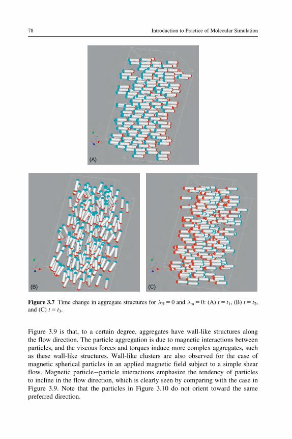
Figure 3.9 is that, to a certain degree, aggregates have wall-like structures along
the flow direction. The particle aggregation is due to magnetic interactions between
particles, and the viscous forces and torques induce more complex aggregates, such
as these wall-like structures. Wall-like clusters are also observed for the case of
magnetic spherical particles in an applied magnetic field subject to a simple shear
flow. Magnetic particle�particle interactions emphasize the tendency of particles
to incline in the flow direction, which is clearly seen by comparing with the case in
Figure 3.9. Note that the particles in Figure 3.10 do not orient toward the same
preferred direction.
(A)
(B) (C)
Figure 3.7 Time change in aggregate structures for λH5 0 and λm5 0: (A) t5 t1, (B) t5 t2,
and (C) t5 t3.
78 Introduction to Practice of Molecular Simulation

Figure 3.11 is a snapshot for a significantly strong applied magnetic field
λH5 50, but without magnetic particle�particle interactions. Since a magnetic
field is significantly strong, each particle inclines to a higher degree in the mag-
netic field direction (y-axis direction) as compared with that in Figure 3.9. On the
other hand, wall-like clusters are not formed in this case because there are no
magnetic interactions.
(A) (B)
Figure 3.8 Aggregate structures for λH5 0 and λm5 10: (A) an oblique view and (B)
viewed nearly from the negative x-axis.
(A) (B)
Figure 3.9 Aggregate structures for λH5 10 and λm5 0: (A) an oblique view and (B)
viewed nearly from the negative x-axis.
79Practice of Molecular Dynamics Simulations

Figure 3.12 also shows λH5 50, as in Figure 3.11, but magnetic interactions are
λm5 10 in this case. Comparison with Figure 3.10, clearly reveals that wall-like
clusters are formed along the flow direction. The detailed observation of the inter-
nal structures of wall-like clusters indicates that the rod-like particles aggregate to
(A) (B)
Figure 3.10 Aggregate structures for λH5 10 and λm5 10: (A) an oblique view and (B)
viewed nearly from the negative x-axis.
(B)(A)
Figure 3.11 Aggregate structures for λH5 50 and λm5 0: (A) an oblique view and (B)
viewed nearly from the negative x-axis.
80 Introduction to Practice of Molecular Simulation

form wall-like structures in such a way that one cluster is placed into two parallel
clusters, with the plus magnetic charge of the center particle in contact with the
minus magnetic charges of the two neighboring particles.
The above discussion has systematically used snapshots to present the properties
of aggregates. However, this type of qualitative discussion is insufficient for an
academic paper, and the addition of quantitative discussion is necessary. For this
exercise, it would be suitable to discuss the radial, pair, and orientational distribu-
tion functions, whilst further investigation of the phenomena might necessitate
Brownian dynamics in order to include random particle motion.
3.2.9 Simulation Program
The following sample simulation program has been written for the present simula-
tion in FORTRAN. The important variables used in the simulation program are as
follows:
RX(I),RY(I),RZ(I) : (x, y, z) components of the position vector r�i of particle i
NX(I),NY(I),NZ(I) : (x, y, z) components of the unit vector ni(5 ei) of particle i
denoting the particle and magnetic moment direction
FX(I),FY(I),FZ(I) : (x, y, z) components of the force F�i acting on particle i
TX(I),TY(I),TZ(I) : (x, y, z) components of the torque T�i acting on particle i
XL,YL,ZL : Side lengths of the simulation box in the (x, y, z) directions
L : Length l* of the solid part of the spherocylinder particle
D : Diameter d* of the solid cylinder part of the spherocylinder
DEL : Thickness δ* of the surfactant layerTD : Ratio 2δ*(52δ/d) of the surfactant layer thickness to the
particle radius
(A) (B)
Figure 3.12 Aggregate structures for λH5 50 and λm5 10: (A) an oblique view and (B)
viewed nearly from the negative x-axis.
81Practice of Molecular Dynamics Simulations

RP : Particle aspect ratio rp (5l/d)
RP1 : Particle aspect ratio rp0(5l0/d5 rp2 1)
N : Number of particles
VDENS : Volumetric fraction of particles φV
NDENS : Number density of particles
HX,HY,HZ : (x,y,z) components of the unit vector denoting the magnetic
field direction
RAM : Nondimensional parameter λm representing the strength of
magnetic particle�particle interactions
RAH : Nondimensional parameter λH representing the strength of
magnetic particle�field interactions
RAV : Nondimensional parameter λV representing the strength of
repulsive interactions due to the overlap of steric layers
H : Time interval
RCOFF : Cutoff distance for calculations of forces and torques
XA,YA,YC,YH : Resistance functions
GAMDOT : Shear rate _γ�
MOMX(*),MOMY(*),MOMZ(*)
: Averaged values of the particle direction at each time step
As an aid for understanding the program, comments have been added to the impor-
tant features. The line numbers shown at the beginning of each line are just for the
reader’s convenience and are unnecessary for executing the FORTRAN program.
We briefly explain quasi-random numbers, which are used in the subroutine
“INITIAL” for setting an initial configuration. A quasi-random number is generated
using an irrational. For example, ifffiffiffi2
pis used, the fractional parts of
ffiffiffi2
p; 2
ffiffiffi2
p;
3ffiffiffi2
p; 4
ffiffiffi2
p; . . . provide a sequence of quasi-random numbers ranging from zero to
unity.
0001 C*********************************************************************0002 C* mdcylndr1.f *0003 C* *0004 C* OPEN(9, FILE='@bbb1.dat', STATUS='UNKNOWN') *0005 C* OPEN(10,FILE='bbb11.dat', STATUS='UNKNOWN') *0006 C* OPEN(13,FILE='bbb41.mgf', STATUS='UNKNOWN') *0007 C* OPEN(21,FILE='bbb001.dat',STATUS='UNKNOWN') *0008 C* OPEN(22,FILE='bbb011.dat',STATUS='UNKNOWN') *0009 C* OPEN(23,FILE='bbb021.dat',STATUS='UNKNOWN') *0010 C* OPEN(24,FILE='bbb031.dat',STATUS='UNKNOWN') *0011 C* OPEN(25,FILE='bbb041.dat',STATUS='UNKNOWN') *0012 C* OPEN(26,FILE='bbb051.dat',STATUS='UNKNOWN') *0013 C* OPEN(27,FILE='bbb061.dat',STATUS='UNKNOWN') *0014 C* OPEN(28,FILE='bbb071.dat',STATUS='UNKNOWN') *0015 C* OPEN(29,FILE='bbb081.dat',STATUS='UNKNOWN') *0016 C* OPEN(30,FILE='bbb091.dat',STATUS='UNKNOWN') *0017 C* *0018 C* ---------- MOLECULAR DYNAMICS SIMULATIONS --------- *0019 C* THREE-DIMENSIONAL MOLECULAR DYNAMICS SIMULATIONS OF *0020 C* A DISPERSION COMPOSED OF MAGNETIC SPHEROCYLINDERS *0021 C* IN A SIMPLE SHEAR FLOW. *0022 C* *0023 C* 1. RODLIKE MODEL WITH ARBITRARY ASPECT RATIO. *0024 C* 2. NO HYDRODYNAMIC INTERACTIONS AMONG PARTICLES. *0025 C* *0026 C* VER.1 BY A.SATOH , '08 5/23 *0027 C*********************************************************************
82 Introduction to Practice of Molecular Simulation

0056 C NTIMEMX : MAXIMUM NUMBER OF TIME STEP 0057 C0058 C -XL/2 < RX < XL/2 , -YL/2 < RY < YL/2, -ZL/2 < RZ < ZL/2 0059 C---------------------------------------------------------------------0060 C 0061 IMPLICIT REAL*8 (A-H,O-Z), INTEGER (I-N) 0062 C 0063 COMMON /BLOCK1/ RX , RY , RZ 0064 COMMON /BLOCK2/ NX , NY , NZ 0065 COMMON /BLOCK3/ FX , FY , FZ 0066 COMMON /BLOCK4/ TX , TY , TZ 0067 COMMON /BLOCK5/ XL , YL , ZL 0068 COMMON /BLOCK6/ RP , RP1 , D , DEL , TD 0069 COMMON /BLOCK7/ XA , YA , YC , YH 0070 COMMON /BLOCK8/ N , NDENS, VDENS 0071 COMMON /BLOCK9/ H , RCOFF, GAMDOT, DX , CORY 0072 COMMON /BLOCK10/ RAM , RAH , RAV 0073 COMMON /BLOCK11/ HX , HY , HZ 0074 COMMON /BLOCK12/ MOMX , MOMY , MOMZ 0075 COMMON /WORK20/ XRXI , YRYI , ZRZI , XRXJ , YRYJ , ZRZJ 0076 COMMON /WORK21/ FXIJS, FYIJS, FZIJS, FXJIS, FYJIS, FZJIS 0077 COMMON /WORK22/ TXIJS, TYIJS, TZIJS, TXJIS, TYJIS, TZJIS 0078 COMMON /WORK23/ RCOFF2 , RP102 , D1 , D1SQ 0079 COMMON /WORK24/ CF0XA , CF0YA , CT0YC , CE0YHYC 0080 C0081 PARAMETER( NN=1000 , NNS=500000 , PI=3.141592653589793D0 ) 0082 C 0083 REAL*8 NDENS 0084 REAL*8 RX(NN) , RY(NN) , RZ(NN) , NX(NN) , NY(NN) , NZ(NN) 0085 REAL*8 FX(NN) , FY(NN) , FZ(NN) , TX(NN) , TY(NN) , TZ(NN) 0086 REAL MOMX(NNS) , MOMY(NNS) , MOMZ(NNS) 0087 C 0088 REAL*8 BETA 0089 REAL*8 RXI , RYI , RZI , NXI , NYI , NZI , FXI , FYI , FZI 0090 REAL*8 TXI , TYI , TZI , WXI , WYI , WZI , WXIN, WYIN, WZIN0091 REAL*8 FXIP , FYIP , FZIP , FXIN , FYIN , FZIN 0092 REAL*8 TXIP , TYIP , TZIP , TXIN , TYIN , TZIN 0093 REAL*8 OMEIPX , OMEIPY , OMEIPZ , OMEINX , OMEINY , OMEINZ 0094 REAL*8 C1 , C2 , C3 , C00 0095 REAL*8 C1X , C1Y , C1Z , C2X , C2Y , C2Z 0096 REAL*8 C3X , C3Y , C3Z 0097 REAL*8 CCA1 , CCB1 , CCS1 , CCL1 0098 INTEGER NTIME , NTIMEMX , NGRAPH , DNSMPL , NP , NOPT
0028 C N : NUMBER OF PARTICLES 0029 C D : DIAMETER OF SOLID HEMISPHERE PARTICLE (=1) 0030 C L : LENGTH OF SOLID SPHEROCYLINDER 0031 C RP : ASPECT RATIO (=L/D) 0032 C RP1 : ASPECT RATIO OF CYLINDER LENGTH TO D (=RP-1) 0033 C NDENS : NUMBER DENSITY 0034 C VDENS : VOLUMETRIC FRACTION 0035 C RAM : NONDIMENSIONAL PARAMETER OF PARTICLE-PARTICLE INTERACT 0036 C RAH : NONDIMENSIONAL PARAMETER OF PARTICLE-FIELD INTERACTION 0037 C RAV : NONDIMENSIONAL PARAMETER OF STERIC REPULSION 0038 C RCOFF : CUTOFF RADIUS FOR CALCULATION OF INTERACTION ENERGIES 0039 C XL,YL,ZL : DIMENSIONS OF SIMULATION REGION 0040 C BETA : ASPECT RATIO OF SIMULATION BOX 0041 C (HX,HY,HZ) : UNIT VECTOR DENOTING MAGNETIC FIELD DIRECTION 0042 C 0043 C XA,YA : RESISTANCE FUNC. FOR TRANSLATIONAL MOTION 0044 C YC : RESISTANCE FUNC. FOR ROTATIONAL MOTION 0045 C YH : RESISTANCE FUNC. FOR SHEAR FLOW TERM 0046 C RX(I),RY(I),RZ(I) : PARTICLE POSITION 0047 C NX(N),NY(N),NZ(N) : DIRECTION OF PARTICLE MAJOR AXIS AND0048 C MAGNETIC MOMENT 0049 C FX(I),FY(I),FZ(I) : FORCES ACTING ON PARTICLE I 0050 C TX(I),TY(I),TZ(I) : TORQUES ACTING ON PARTICLE I 0051 C MOMX(**),MOMY(**) : MAG. MOMENT OF SYSTEM AT EACH TIME STEP 0052 C MOMZ(**) 0053 C 0054 C H : INTERVAL OF TIME STEP FOR MOLE. DYNA. SIMULATIONS 0055 C GAMDOT : SHEAR RATE (=1 FOR THIS CASE)
83Practice of Molecular Dynamics Simulations

0111 OPEN(27,FILE='bbb061.dat',STATUS='UNKNOWN') 0112 OPEN(28,FILE='bbb071.dat',STATUS='UNKNOWN') 0113 OPEN(29,FILE='bbb081.dat',STATUS='UNKNOWN') 0114 OPEN(30,FILE='bbb091.dat',STATUS='UNKNOWN') 0115 NP=90116 C 0117 C --- PARAMETER (1) ---0118 C -------------------------------------------------0119 C N=5**3(125), 6**3(216), 7**3(343), 8**3(512) 0120 C -------------------------------------------------0121 C RAH = 0.1 1.0 10. 100. 0122 C H = 0.001 0.001 0.001 0.0001 0123 C ++++++++++++++++++++++++++++++++ 0124 C RAM = 0.1 1.0 10. 100. 0125 C H = 0.001 0.001 0.001 0.00010126 C0127 C THE MINIMUM VALUE ON THE ABOVE LIST MUST BE 0128 C USED FOR THE TIME INTERVAL H.0129 C -------------------------------------------------0130 N = 216 0131 VDENS = 0.05D0 0132 RAM = 20.D0 0133 RAH = 10.0D0 0134 RAV = 150.D0 0135 RP = 5.D0 0136 RP1 = RP - 1.D0 0137 C --- PARAMETER (2) ---0138 H = 0.0001D0 0139 GAMDOT = 1.D0 0140 TD = 0.3D0 0141 RCOFF = 5.D0*RP0142 DEL = TD/2.D0 0143 HX = 0.D0 0144 HY = 1.D0 0145 HZ = 0.D0 0146 C --- PARAMETER (3) ---0147 BETA = 2.D0 0148 DX = 0.D0 0149 D = 1.0D00150 NDENS = ( 12.D0/( PI*(3.D0*RP-1.D0) ) )*VDENS 0151 C --- PARAMETER (4) ---0152 NTIMEMX = 200000 0153 NGRAPH = NTIMEMX/10 0154 NANIME = NTIMEMX/200 0155 DNSMPL = 2 0156 NOPT = 20 0157 C --- PARAMETER (5) ---0158 CCA1 = RP/2.D0 + DEL 0159 CCB1 = 0.5D0 + DEL0160 CCS1 = DSQRT( CCA1**2 - CCB1**2 ) / CCA1 0161 CCL1 = DLOG( (1.D0+CCS1)/(1.D0-CCS1) ) 0162 XA = (8.D0/3.D0)*CCS1**30163 & / ( -2.D0*CCS1+(1.D0+CCS1**2)*CCL1 ) 0164 YA = (16.D0/3.D0)*CCS1**3 0165 & / ( 2.D0*CCS1+(3.D0*CCS1**2-1.D0)*CCL1 )
• The particle number N=216, volu- metric fraction φV =0.05, λm=20, λH= 10, λV=150, and aspect ratio rp=5.
• The time interval h*=0.0001, tδ=0.3, cutoff radius r*coff=5rp, thickness of a surfactant layer δ*=0.15, and magnetic field direction h=(0,1,0).
• BETA is used in determining the simulation regionsize. NDENS is the number density of particles.
• The main loop is finished when NTIME arrives at 200,000.• The particle position and other data are written out at every NGRAPH time steps. 200 sets of data are written out for making an animation based on MicroAVS.
• The resistance functions XA, YA, YC,and YH are calculated in advance.
0099 INTEGER NSMPL1 , NSMPL2 0100 INTEGER NANIME , NANMCTR, NOPT1 0101 C 0102 OPEN(9,FILE='@bbb1.dat' , STATUS='UNKNOWN') 0103 OPEN(10,FILE='bbb11.dat', STATUS='UNKNOWN') 0104 OPEN(13,FILE='bbb41.mgf', STATUS='UNKNOWN') 0105 OPEN(21,FILE='bbb001.dat',STATUS='UNKNOWN') 0106 OPEN(22,FILE='bbb011.dat',STATUS='UNKNOWN') 0107 OPEN(23,FILE='bbb021.dat',STATUS='UNKNOWN') 0108 OPEN(24,FILE='bbb031.dat',STATUS='UNKNOWN') 0109 OPEN(25,FILE='bbb041.dat',STATUS='UNKNOWN') 0110 OPEN(26,FILE='bbb051.dat',STATUS='UNKNOWN')
• The given values and the magnetic moment results are written out in @bbb1 and bbb11, the data for MicroAVS are done in bbb41, and the intermedi-ate positions and directions are done in bbb001–bbb091 in the time sequential order.
0166 YC = (4.D0/3.D0)* ( CCS1**3*(2.D0-CCS1**2) ) 0167 & / ( -2.D0*CCS1+(1.D0+CCS1**2)*CCL1 ) 0168 YH = (4.D0/3.D0)*CCS1**5 0169 & / ( -2.D0*CCS1+(1.D0+CCS1**2)*CCL1 )
84 Introduction to Practice of Molecular Simulation

0170 C --- PARAMETER (6) ---0171 RCOFF2 = RCOFF**20172 RP102 = RP1/2.D0 0173 D1 = 1.D0+TD 0174 D1SQ = D1**2 0175 CF0XA = 1.D0/( XA*(RP+2.D0*DEL ) ) 0176 CF0YA = 1.D0/( YA*(RP+2.D0*DEL ) ) 0177 CT0YC = 1.D0/( YC*(RP+2.D0*DEL )**3 )0178 CE0YHYC = (YH/YC)*0.5D0 0179 C 0180 C ----------------------------------------------------------------0181 C ----------------- INITIAL CONFIGURATION ------------------0182 C ----------------------------------------------------------------0183 C 0184 C --- SET INITIAL CONFIG. ---0185 CCC OPEN(19,FILE='qqq091.dat',STATUS='OLD') 0186 CCC READ(19,472) N , XL , YL , ZL , D , TD , RP , RP1 , DX 0187 CCC READ(19,474) (RX(I),I=1,N),(RY(I),I=1,N),(RZ(I),I=1,N),0188 CCC & (NX(I),I=1,N),(NY(I),I=1,N),(NZ(I),I=1,N)0189 CCC CLOSE(19,STATUS='KEEP') 0190 CCC GOTO 7 0191 C 0192 CALL INITIAL( BETA ) 0193 C 0194 7 IF( RCOFF .GE. XL/2.D0 ) THEN 0195 RCOFF = XL/2.D0 - 0.00001D00196 END IF0197 RCOFF2 = RCOFF**2 0198 C --- CAL FORCES ---0199 NTIME = 0 0200 CALL FORCECAL( NP, NTIME )0201 C 0202 C --- PRINT OUT ---0203 WRITE(NP,12) N, VDENS, NDENS, RAM ,RAH ,RAV, RP, RP1, D, DEL, 0204 & TD, XA, YA, YC, YH, H, RCOFF, GAMDOT, BETA, 0205 & XL, YL, ZL 0206 WRITE(NP,13) RP102, D1, CF0XA, CF0YA, CT0YC, CE0YHYC 0207 WRITE(NP,14) NTIMEMX, NGRAPH, DNSMPL0208 C 0209 C --- INITIALIZATION ---0210 NANMCTR = 00211 NSMPL = 0 0212 C 0213 C ----------------------------------------------------------------0214 C ------------------ START OF MAIN LOOP --------------------0215 C ----------------------------------------------------------------0216 C 0217 DO 1000 NTIME = 1,NTIMEMX 0218 C 0219 DX = GAMDOT*YL*H*DBLE(NTIME) 0220 DX = DMOD( DX, XL )
• CF0XA and CF0YA are the coefficients in the force term in Eq. (3.49), CT0YC is the coefficient in the torque term in Eq. (3.50), and CE0YHYC is a part of the coefficient ofthe shear rate in Eq. (3.50).
• These READ statements are for continuing the sequentialsimulation using the data saved previously.
• The particle initial positions and velocities are assigned .
• The forces and torques acting between particlesare calculated.
• DX is ΔX in Fig. 2.15.
0221 C 0222 DO 100 I = 1,N 0223 C 0224 NXI = NX(I) 0225 NYI = NY(I) 0226 NZI = NZ(I) 0227 FXI = FX(I) 0228 FYI = FY(I) 0229 FZI = FZ(I) 0230 TXI = TX(I) 0231 TYI = TY(I) 0232 TZI = TZ(I) 0233 C --- (1) TRANSLATIONAL MOTION ---0234 C0235 C00 = FXI*NXI + FYI*NYI + FZI*NZI 0236 FXIP = C00*NXI 0237 FYIP = C00*NYI 0238 FZIP = C00*NZI 0239 FXIN = FXI - FXIP 0240 FYIN = FYI - FYIP
• The force acting on particle i is decomposed into one in the particle direction and another in the direction normal to the particle axis according to Eq. (3.36).
85Practice of Molecular Dynamics Simulations

0241 FZIN = FZI - FZIP 0242 C0243 RXI = RX(I) + H*( CF0XA*FXIP+CF0YA*FXIN ) + RY(I)*GAMDOT*H0244 RYI = RY(I) + H*( CF0XA*FYIP+CF0YA*FYIN ) 0245 RZI = RZ(I) + H*( CF0XA*FZIP+CF0YA*FZIN ) 0246 CORY = DNINT( RYI/YL ) 0247 RXI = RXI - CORY*DX 0248 RX(I) = RXI - DNINT( RXI/XL )*XL 0249 RY(I) = RYI - CORY*YL 0250 RZ(I) = RZI - DNINT( RZI/ZL )*ZL 0251 C 0252 C --- (2) ROTATIONAL MOTION ---0253 C00 = TXI*NXI + TYI*NYI + TZI*NZI 0254 TXIP = C00*NXI 0255 TYIP = C00*NYI 0256 TZIP = C00*NZI 0257 TXIN = TXI - TXIP 0258 TYIN = TYI - TYIP 0259 TZIN = TZI - TZIP 0260 C0261 C00 = -0.5D0*NZI 0262 OMEIPX = C00*NXI 0263 OMEIPY = C00*NYI 0264 OMEIPZ = C00*NZI 0265 OMEINX = - OMEIPX 0266 OMEINY = - OMEIPY 0267 OMEINZ = -0.5D0 - OMEIPZ 0268 C0269 C1X = CT0YC*TXIN 0270 C1Y = CT0YC*TYIN 0271 C1Z = CT0YC*TZIN 0272 C2X = -CE0YHYC* ( NZI*NXI ) 0273 C2Y = -CE0YHYC* (-NZI*NYI ) 0274 C2Z = -CE0YHYC* ( NYI**2 - NXI**2 )
• This is the treatment of the Lees–Edwards BC explained in Section 2.4.2.
• The torque acting on particle i is decomposed into one about the particle direction and another about a line normal to the particle direction through its center according to Eq. (3.36).
• The angular velocity is decomposed into twovectors in a similar way to the torque.
• The terms of the torque and the shear rate are calculated in the angular velocity in Eq. (3.50).
0275 C 0276 WXIN = OMEINX + C1X + C2X 0277 WYIN = OMEINY + C1Y + C2Y 0278 WZIN = OMEINZ + C1Z + C2Z 0279 C3X = WYIN*NZI - WZIN*NYI 0280 C3Y = WZIN*NXI - WXIN*NZI 0281 C3Z = WXIN*NYI - WYIN*NXI 0282 C0283 NXI = NXI + H*C3X 0284 NYI = NYI + H*C3Y 0285 NZI = NZI + H*C3Z 0286 C00 = DSQRT( NXI**2 + NYI**2 + NZI**2 ) 0287 NX(I) = NXI/C00 0288 NY(I) = NYI/C00 0289 NZ(I) = NZI/C00 0290 C 0291 100 CONTINUE 0292 C --- CAL FORCES ---0293 CALL FORCECAL( NP, NTIME )0294 C 0295 C ----------------------------------------------------------------0296 C --- MOMENT OF SYSTEM ---0297 IF( MOD(NTIME,DNSMPL) .EQ. 0 ) THEN 0298 NSMPL = NSMPL + 1 0299 C1 = 0.D0 0300 C2 = 0.D0 0301 C3 = 0.D0 0302 DO 450 J=1,N 0303 C1 = C1 + NX(J) 0304 C2 = C2 + NY(J) 0305 C3 = C3 + NZ(J) 0306 450 CONTINUE 0307 MOMX(NSMPL) = REAL(C1)/REAL(N) 0308 MOMY(NSMPL) = REAL(C2)/REAL(N) 0309 MOMZ(NSMPL) = REAL(C3)/REAL(N) 0310 END IF
• The angular velocity in Eq.(3.50) is calculated.
• To evaluate the particle direction from Eq.(3.55), the vector product of the angular velocity and the particle direction is first calculated.
• The particle direction is evaluated from Eq. (3.55).
• The modification is made to yield the unit vector.
• Calculation of the forces and torques.
• To check the system convergence afterward, the average of the particledirection vector is calculated.
• The data of the particle positions anddirections are written out at every NGRAPH time steps for the post processing analysis.
0311 C 0312 C --- DATA OUTPUT (1) FOR GRAPHICS ---
86 Introduction to Practice of Molecular Simulation

0313 IF( MOD(NTIME,NGRAPH) .EQ. 0 ) THEN 0314 NOPT = NOPT + 1 0315 WRITE(NOPT,472) N , XL , YL , ZL , D , TD , RP , RP1 , DX 0316 WRITE(NOPT,474) (RX(I),I=1,N),(RY(I),I=1,N),(RZ(I),I=1,N),0317 & (NX(I),I=1,N),(NY(I),I=1,N),(NZ(I),I=1,N)0318 CLOSE(NOPT,STATUS='KEEP') 0319 END IF 0320 C0321 C --- DATA OUTPUT FOR ANIMATION (2) ---0322 IF( MOD(NTIME,NANIME) .EQ. 0 ) THEN0323 NANMCTR = NANMCTR + 10324 NOPT1 = 13 0325 CALL DATAOPUT( NOPT1, NANMCTR, NTIMEMX, NANIME, N ) 0326 END IF 0327 C 0328 C 0329 1000 CONTINUE
• The data of the particle positions and directions are written out at everyNANIME time steps for making an animation based on MicroAVS.
0330 C 0331 C ----------------------------------------------------------------0332 C ------------------- END OF MOLECULAR DYNAMICS ---------------0333 C ----------------------------------------------------------------0334 C 0335 C --- PRINT OUT (2) ---0336 WRITE(NP,1011) 0337 NSMPL1 = 10338 NSMPL2 = NSMPL 0339 CALL PRNTDATA( NSMPL1 , NSMPL2 , NP ) 0340 WRITE(NP,1013) NSMPL1 , NSMPL2 0341 C --- DATA OUTPUT (2) FOR GRAPHICS ---0342 WRITE(10,1111) N, VDENS, NDENS, RAM, RAH, RAV 0343 WRITE(10,1113) RP, RP1, D, DEL, TD, XA, YA, YC, YH 0344 WRITE(10,1115) H, RCOFF, GAMDOT, BETA, XL, YL, ZL 0345 WRITE(10,1117) RP102, D1, CF0XA, CF0YA, CT0YC, CE0YHYC 0346 WRITE(10,1119) NTIMEMX, NGRAPH, DNSMPL 0347 WRITE(10,1121) ( MOMX(I),I=NSMPL1, NSMPL2) 0348 & ,( MOMY(I),I=NSMPL1, NSMPL2) 0349 & ,( MOMZ(I),I=NSMPL1, NSMPL2) 0350 C0351 CLOSE(9, STATUS='KEEP') 0352 CLOSE(10,STATUS='KEEP') 0353 CLOSE(13,STATUS='KEEP') 0354 C -------------------------- FORMAT ------------------------------0355 12 FORMAT(/1H ,'--------------------------------------------------'0356 & /1H ,'- MOLECULAR DYNAMICS SIMULATIONS OF SPHERO- -'0357 & /1H ,'- CYLINDER PARTICLES IN A SIMPLE SHEAR FLOW -'0358 & /1H ,'--------------------------------------------------'0359 & //1H ,'N=',I6, 2X, 'VDENS=',F7.4, 2X ,'NDENS=',F9.6 0360 & /1H ,'RAM=',F6.2, 2X, 'RAH=',F6.2, 2X ,'RAV=',F7.2 0361 & /1H ,'RP=',F5.2, 2X ,'RP1=',F5.2, 2X ,'D=',F5.2, 2X ,0362 & 'DEL=',F5.2, 2X,'TD=',F5.20363 & /1H ,'XA=',E12.4,2X,'YA=',E12.4,2X,'YC=',E12.4,2X,0364 & 'YH=',E12.40365 & /1H ,'H=',E12.4,3X,'RCOFF=',F5.2,2X,'GAMDOT=',F5.2,2X,0366 & 'BETA=', F5.20367 & /1H ,'XL=',F6.2,2X,'YL=',F6.2,2X,'ZL=',F6.2) 0368 13 FORMAT( 1H ,'RP102=',F5.2,2X,'D1=',F5.2,2X,0369 & 'CF0XA=',E11.3, 2X, 'CF0YA=',E11.30370 & /1H ,'CT0YC=',E11.3, 2X, 'CE0YHYC=',E11.3)0371 14 FORMAT( 1H ,'NTIMEMX=',I8, 2X,'NGRAPH=',I8,2X,'DNSMPL=',I8/)0372 472 FORMAT( I5 , 3F9.4 , 4F8.4 , E16.8 ) 0373 474 FORMAT( (5F16.10) ) 0374 1011 FORMAT(/1H ,'++++++++++++++++++++++++++++++' 0375 & /1H ,' MD SIMULATIONS ' 0376 & /1H ,'++++++++++++++++++++++++++++++'/) 0377 1013 FORMAT(///1H ,18X, 'START OF MD SAMPLING STEP=',I7 0378 & /1H ,18X, 'END OF MD SAMPLING STEP=',I7/) 0379 1111 FORMAT( I5 , 2F7.4 , 3F12.5 ) 0380 1113 FORMAT( 3F6.2 , 2F7.3 , 4E12.4 ) 0381 1115 FORMAT( E11.3 , F8.3 , 2F7.4 , 3F9.3 ) 0382 1117 FORMAT( 2F6.2 , 4E12.4 ) 0383 1119 FORMAT( 3I8 ) 0384 1121 FORMAT( (10F8.5) )
• To check the system convergence afterward, the data of the particle directions are written out.
87Practice of Molecular Dynamics Simulations

0385 STOP0386 END 0387 C*********************************************************************0388 C*************************** SUBROUTINE **************************0389 C*********************************************************************0390 C 0391 C**** SUB PRNTDATA **** 0392 SUBROUTINE PRNTDATA( MCSST, MCSMX, NP ) 0393 C 0394 IMPLICIT REAL*8 (A-H,O-Z), INTEGER (I-N) 0395 C 0396 COMMON /BLOCK12/ MOMX , MOMY , MOMZ 0397 C 0398 PARAMETER( NN=1000 , NNS=500000 , PI=3.141592653589793D0 ) 0399 C 0400 INTEGER MCSST , MCSMX , NP 0401 REAL MOMX(NNS) , MOMY(NNS) , MOMZ(NNS) 0402 C 0403 REAL AMOMX(10) , AMOMY(10) , AMOMZ(10) , C0 0404 INTEGER IC , IMC(0:10) , JS , JE 0405 C 0406 C ----- KEIKA INSATU -----0407 IC = ( MCSMX-MCSST+1 )/50 0408 DO 20 I= MCSST-1+IC , MCSMX , IC 0409 WRITE(NP,10) I, MOMX(I), MOMY(I), MOMZ(I) 0410 20 CONTINUE 0411 C ----- TIME STEP HEIKIN -----0412 IC = ( MCSMX-MCSST+1 )/10 0413 DO 30 I=0,10 0414 IMC(I) = MCSST - 1 + IC*I 0415 IF( I .EQ. 10 ) IMC(I) =MCSMX 0416 30 CONTINUE 0417 C 0418 C 0419 DO 35 I=1,10 0420 AMOMX( I) = 0. 0421 AMOMY( I) = 0. 0422 AMOMZ( I) = 0. 0423 35 CONTINUE 0424 C 0425 DO 50 I=1,10 0426 JS = IMC(I-1) + 1 0427 JE = IMC(I) 0428 DO 40 J=JS,JE 0429 AMOMX(I) = AMOMX(I) + MOMX( J) 0430 AMOMY(I) = AMOMY(I) + MOMY( J) 0431 AMOMZ(I) = AMOMZ(I) + MOMZ( J) 0432 40 CONTINUE 0433 50 CONTINUE 0434 C 0435 DO 70 I=1,10 0436 C0 = REAL( IMC(I)-IMC(I-1) ) 0437 AMOMX(I) = AMOMX(I) /C0 0438 AMOMY(I) = AMOMY(I) /C0 0439 AMOMZ(I) = AMOMZ(I) /C0
• The total time steps are equally divided into 50 blocks, and the end value of each block is written out.
• The total time steps are equally divided into 10 blocks, and the subaverages are calculated for each block.
0440 70 CONTINUE 0441 C ----- STEP HEIKIN INSATU -----0442 WRITE(NP,75) 0443 DO 90 I=1,10 0444 WRITE(NP,80) I, IMC(I-1)+1, IMC(I), AMOMX(I),AMOMY(I),AMOMZ(I)0445 90 CONTINUE 0446 C ----------------------------------------------------------------0447 10 FORMAT(1H ,'SMPL=',I7, 1X ,'NX=',F6.3, 1X,'NY=',F6.3, 0448 & 1X,'NZ=',F6.3)0449 75 FORMAT(//1H ,'-----------------------------------------------' 0450 & /1H ,' TIME AVERAGE ' 0451 & /) 0452 80 FORMAT(1H ,'I=',I2, 2X ,'SMPLMN=',I7, 2X ,'SMPLMX=',I7 0453 & /1H ,5X ,'NX=',F6.3, 2X,'NY=',F6.3, 2X,'NZ=',F6.3/) 0454 RETURN0455 END 0456 C**** SUB INITIAL ****
88 Introduction to Practice of Molecular Simulation

0457 SUBROUTINE INITIAL( BETA ) 0458 C 0459 IMPLICIT REAL*8 (A-H,O-Z), INTEGER (I-N) 0460 C0461 COMMON /BLOCK1/ RX , RY , RZ 0462 COMMON /BLOCK2/ NX , NY , NZ 0463 COMMON /BLOCK5/ XL , YL , ZL 0464 COMMON /BLOCK6/ RP , RP1 , D , DEL , TD 0465 COMMON /BLOCK8/ N , NDENS, VDENS 0466 COMMON /BLOCK9/ H , RCOFF, GAMDOT, DX , CORY 0467 C0468 PARAMETER( NN=1000 , PI=3.141592653589793D0 ) 0469 C 0470 REAL*8 NDENS 0471 REAL*8 RX(NN) , RY(NN) , RZ(NN) , NX(NN) , NY(NN) , NZ(NN) 0472 C 0473 INTEGER Q , PTCL 0474 REAL*8 A , XLUNT , YLUNT , ZLUNT, RAN1 , RAN2 , RAN30475 REAL*8 C1 , C2 , C3 0476 C 0477 A = 1.D0/( (BETA*NDENS)**(1./3.) ) 0478 Q = NINT( (REAL(N+1))**(1./3.) ) 0479 XL = A*DBLE(Q)0480 YL = A*DBLE(Q)*BETA0481 ZL = A*DBLE(Q)0482 XLUNT = A0483 YLUNT = A*BETA 0484 ZLUNT = A0485 C ----- POSITION ----- 0486 RAN1 = DSQRT( 2.D0 ) 0487 RAN2 = DSQRT( 7.D0 ) 0488 RAN3 = DSQRT( 11.D0 ) 0489 PTCL = 0 0490 DO 10 K=0,Q-1 0491 DO 10 J=0,Q-1 0492 DO 10 I=0,Q-1 0493 PTCL = PTCL + 1 0494 C1 = RAN1*DBLE(PTCL)
• A subroutine for setting the initial positions and velocities of particles.
• The volume occupied by one particle is βa*3 and therefore a*=1/(βn*)1/3 because of βa*3n*=1 (n* is the number density).• The side lengths of the unit cell are (a*, βa* , a*) in each direction.
• RAN1, RAN2, and RAN3 are quasi-random numbers. • Q particles are located in each axis direction. • Each particle is moved in parallel by (XLUNT/3, YLUNT/3, ZLUNT/3) to remove subtle situations at outer boundary surfaces. Also, to remove the regularity of the initial configu-ration, each particle is moved randomly by the maximum displacement (1/2)×(XLUNT/8, YLUNT/8, ZLUNT/8) using quasi-random numbers.• Each particle is moved in parallel by (1/2)×(-XL, -YL, -ZL), so that the simulation box center is the coordinate origin.
0495 C1 = C1 - DINT(C1) 0496 C1 = C1 - 0.5D0 0497 C2 = RAN2*DBLE(PTCL) 0498 C2 = C2 - DINT(C2) 0499 C2 = C2 - 0.5D0 0500 C3 = RAN3*DBLE(PTCL) 0501 C3 = C3 - DINT(C3) 0502 C3 = C3 - 0.5D0 0503 RX(PTCL) = DBLE(I)*XLUNT+XLUNT/3D0+C1*(XLUNT/8.D0)-XL/2.D0 0504 RY(PTCL) = DBLE(J)*YLUNT+YLUNT/3D0+C2*(YLUNT/8.D0)-YL/2.D0 0505 RZ(PTCL) = DBLE(K)*ZLUNT+ZLUNT/3D0+C3*(ZLUNT/8.D0)-ZL/2.D0 0506 10 CONTINUE 0507 N = PTCL 0508 C ----- MOMENT -----0509 RAN1 = DSQRT( 2.D0 ) 0510 RAN2 = DSQRT( 3.D0 ) 0511 DO 20 I=1,N 0512 C1 = RAN1*DBLE(I) 0513 C1 = C1 - DINT(C1)0514 C1 = C1 - 0.5D0 0515 C1 = PI/2.D0 + (5.D0/180.D0)*PI*C1 0516 C2 = RAN2*DBLE(I) 0517 C2 = C2 - DINT(C2)0518 C2 = C2 - 0.5D0 0519 C2 = PI/2.D0 + (5.D0/180.D0)*PI*C2 0520 NX(I) = DSIN(C1)*DCOS(C2) 0521 NY(I) = DSIN(C1)*DSIN(C2) 0522 NZ(I) = DCOS(C1) 0523 20 CONTINUE 0524 RETURN 0525 END 0526 C**** SUB DATAOPUT **** 0527 SUBROUTINE DATAOPUT( NOPT1, NANMCTR, NTIMEMX, NANIME, N ) 0528 C
• The initial direction of each particle is randomly assigned with a certain angle range about the y-direction using quasi-random numbers.
89Practice of Molecular Dynamics Simulations

0529 IMPLICIT REAL*8 (A-H,O-Z), INTEGER (I-N) 0530 C0531 COMMON /BLOCK1/ RX , RY , RZ 0532 COMMON /BLOCK2/ NX , NY , NZ 0533 COMMON /BLOCK5/ XL , YL , ZL 0534 COMMON /BLOCK6/ RP , RP1 , D , DEL , TD 0535 COMMON /BLOCK9/ H , RCOFF, GAMDOT, DX , CORY 0536 C0537 PARAMETER( NN=1000 , PI=3.141592653589793D0 ) 0538 C 0539 REAL*8 RX(NN) , RY(NN) , RZ(NN) , NX(NN) , NY(NN) , NZ(NN) 0540 REAL*8 RP102 , CRADIUS , CX1 , CY1 , CZ1 , CX2 , CY2 , CZ2 0541 C 0542 RP102 = RP1/2.D0 0543 CRADIUS = ( D + TD )/2.D00544 XL2 = XL/2.D0 0545 YL2 = YL/2.D0 0546 ZL2 = ZL/2.D0 0547 C0548 IF( NANMCTR .EQ. 1 ) THEN 0549 WRITE(NOPT1,181) ( NTIMEMX/NANIME )
• A subroutine for writing out the data which can be used for making an animation based on the commercial software MicroAVS.
• MicroAVS can make a visualiza- tion or animation by reading the data from bbb41.mgf.
0550 END IF0551 C0552 IF( (NANMCTR.GE.1) .AND. (NANMCTR.LE.9) ) THEN 0553 WRITE(NOPT1,183) NANMCTR0554 ELSE IF( (NANMCTR.GE.10) .AND. (NANMCTR.LE.99) ) THEN 0555 WRITE(NOPT1,184) NANMCTR0556 ELSE IF( (NANMCTR.GE.100) .AND. (NANMCTR.LE.999) ) THEN 0557 WRITE(NOPT1,185) NANMCTR0558 ELSE IF( (NANMCTR.GE.1000) .AND. (NANMCTR.LE.9999) ) THEN 0559 WRITE(NOPT1,186) NANMCTR0560 END IF 0561 C0562 C ----------------------------------------------- CYLINDER (1) ---0563 WRITE(NOPT1,211) N0564 DO 250 I=1,N 0565 CX1 = RX(I) - NX(I)*RP1020566 CY1 = RY(I) - NY(I)*RP1020567 CZ1 = RZ(I) - NZ(I)*RP1020568 CX2 = RX(I) + NX(I)*RP1020569 CY2 = RY(I) + NY(I)*RP1020570 CZ2 = RZ(I) + NZ(I)*RP1020571 WRITE(NOPT1,248) CX1, CY1, CZ1, CX2, CY2, CZ2, (CRADIUS+1.D-5)0572 250 CONTINUE0573 C 0574 C ------------------------------------------- SPHERE MINUS (2) ---0575 WRITE(NOPT1,311) N0576 DO 350 I=1,N 0577 CX1 = RX(I) - NX(I)*RP1020578 CY1 = RY(I) - NY(I)*RP1020579 CZ1 = RZ(I) - NZ(I)*RP1020580 WRITE(NOPT1,348) CX1, CY1, CZ1, CRADIUS, 0.0, 0.8, 1.0 0581 350 CONTINUE0582 C 0583 C -------------------------------------------- SPHERE PLUS (3) ---0584 WRITE(NOPT1,311) N0585 DO 450 I=1,N 0586 CX1 = RX(I) + NX(I)*RP1020587 CY1 = RY(I) + NY(I)*RP1020588 CZ1 = RZ(I) + NZ(I)*RP1020589 WRITE(NOPT1,348) CX1, CY1, CZ1, CRADIUS, 1.0, 0.0, 0.0 0590 450 CONTINUE0591 C 0592 C -------------------------------------- SIM.REGEON LINES (4) ---0593 WRITE(NOPT1,648) 170594 WRITE(NOPT1,649) -XL2, -YL2, -ZL2 0595 WRITE(NOPT1,649) XL2, -YL2, -ZL2 0596 WRITE(NOPT1,649) XL2, YL2, -ZL2 0597 WRITE(NOPT1,649) -XL2, YL2, -ZL2
• Drawing of the cylindrical part ofparticles.
• Drawing of the hemisphere of thenegative charge.
• Drawing of the hemisphere of thepositive charge.
• Drawing of the frame of thesimulation box.
0598 WRITE(NOPT1,649) -XL2, -YL2, -ZL2 0599 WRITE(NOPT1,649) -XL2, -YL2, ZL2 0600 WRITE(NOPT1,649) XL2, -YL2, ZL2
90 Introduction to Practice of Molecular Simulation

0601 WRITE(NOPT1,649) XL2, YL2, ZL2 0602 WRITE(NOPT1,649) -XL2, YL2, ZL2 0603 WRITE(NOPT1,649) -XL2, -YL2, ZL2 0604 WRITE(NOPT1,649) -XL2, -YL2, -ZL2 0605 WRITE(NOPT1,649) -XL2, YL2, -ZL2 0606 WRITE(NOPT1,649) -XL2, YL2, ZL2 0607 WRITE(NOPT1,649) XL2, YL2, ZL2 0608 WRITE(NOPT1,649) XL2, YL2, -ZL2 0609 WRITE(NOPT1,649) XL2, -YL2, -ZL2 0610 WRITE(NOPT1,649) XL2, -YL2, ZL2 0611 C 0612 C ---------------------------- FORMAT ----------------------------0613 181 FORMAT('# Micro AVS Geom:2.00'0614 & /'# Animation of DPD simulation results'0615 & /I4)0616 183 FORMAT('step',I1) 0617 184 FORMAT('step',I2) 0618 185 FORMAT('step',I3) 0619 186 FORMAT('step',I4) 0620 211 FORMAT( 'column'/'cylinder'/'dvertex'/'32'/I7 ) 0621 248 FORMAT( 6F10.3 , F6.2 )0622 311 FORMAT( 'sphere'/'sphere_sample'/'color'/I7 ) 0623 348 FORMAT( 3F10.3 , F6.2 , 3F5.2 )0624 648 FORMAT( 'polyline'/'pline_sample'/'vertex'/I3 ) 0625 649 FORMAT( 3F10.3 )0626 RETURN 0627 END 0628 C**** SUB FORCECAL ***** 0629 SUBROUTINE FORCECAL( NP, NTIME )0630 C 0631 IMPLICIT REAL*8 (A-H,O-Z), INTEGER (I-N) 0632 C 0633 COMMON /BLOCK1/ RX , RY , RZ 0634 COMMON /BLOCK2/ NX , NY , NZ 0635 COMMON /BLOCK3/ FX , FY , FZ 0636 COMMON /BLOCK4/ TX , TY , TZ 0637 COMMON /BLOCK5/ XL , YL , ZL 0638 COMMON /BLOCK6/ RP , RP1 , D , DEL , TD 0639 COMMON /BLOCK7/ XA , YA , YC , YH 0640 COMMON /BLOCK8/ N , NDENS, VDENS 0641 COMMON /BLOCK9/ H , RCOFF, GAMDOT, DX , CORY 0642 COMMON /BLOCK10/ RAM , RAH , RAV 0643 COMMON /BLOCK11/ HX , HY , HZ 0644 COMMON /WORK20/ XRXI , YRYI , ZRZI , XRXJ , YRYJ , ZRZJ 0645 COMMON /WORK21/ FXIJS, FYIJS, FZIJS, FXJIS, FYJIS, FZJIS 0646 COMMON /WORK22/ TXIJS, TYIJS, TZIJS, TXJIS, TYJIS, TZJIS 0647 COMMON /WORK23/ RCOFF2 , RP102 , D1 , D1SQ 0648 COMMON /WORK24/ CF0XA , CF0YA , CT0YC , CE0YHYC 0649 C0650 PARAMETER( NN=1000 , PI=3.141592653589793D0 ) 0651 C 0652 REAL*8 NDENS 0653 REAL*8 RX(NN) , RY(NN) , RZ(NN) , NX(NN) , NY(NN) , NZ(NN) 0654 REAL*8 FX(NN) , FY(NN) , FZ(NN) , TX(NN) , TY(NN) , TZ(NN) 0655 C 0656 REAL*8 RXI , RYI , RZI , RXIJ , RYIJ , RZIJ , RIJSQ , RIJ 0657 REAL*8 RXJ , RYJ , RZJ 0658 REAL*8 NXI , NYI , NZI , NXIJ , NYIJ , NZIJ 0659 REAL*8 NXJ , NYJ , NZJ , NXIJ2, NYIJ2, NZIJ2
• A subroutine for calculating the forces and torques acting betweenparticles.
0660 REAL*8 FXI , FYI , FZI , TXI , TYI , TZI 0661 REAL*8 FXIJP01 , FYIJP01, FZIJP01, FXIJP02, FYIJP02, FZIJP020662 REAL*8 FXIJM01 , FYIJM01, FZIJM01, FXIJM02, FYIJM02, FZIJM020663 REAL*8 FXIJP , FYIJP , FZIJP , FXJIP , FYJIP , FZJIP 0664 REAL*8 TXIJP , TYIJP , TZIJP , TXJIP , TYJIP , TZJIP 0665 REAL*8 FXIJM , FYIJM , FZIJM , FXJIM , FYJIM , FZJIM 0666 REAL*8 TXIJM , TYIJM , TZIJM , TXJIM , TYJIM , TZJIM 0667 REAL*8 TXIJ , TYIJ , TZIJ , TXIJ0 , TYIJ0 , TZIJ0 0668 REAL*8 XI , YI , ZI , XJ , YJ , ZJ 0669 REAL*8 RRXI , RRYI , RRZI , RRXIJ , RRYIJ , RRZIJ , RRIJ 0670 REAL*8 RRXJ , RRYJ , RRZJ , RCHKSQ, RCHKSQ2 0671 REAL*8 RRXIC , RRYIC , RRZIC , RRXJC , RRYJC , RRZJC 0672 REAL*8 NNXI , NNYI , NNZI , NNXJ , NNYJ , NNZJ
91Practice of Molecular Dynamics Simulations

0673 REAL*8 R11 , R12 , R21 , R22 0674 REAL*8 KI , KJ , KKI , KKJ , KIS , KJS , KKIS , KKIS2 0675 REAL*8 CKI , CKJ , CKKI, CKKJ0676 REAL*8 KKIC, KKJC , CKKIC , CKKIC2 0677 REAL*8 CNINJ , CRIJNI , CRIJNJ , CRIJSQ , CWIDTH 0678 REAL*8 C01X, C01Y, C01Z 0679 REAL*8 C11X, C11Y, C11Z, C12X, C12Y, C12Z 0680 REAL*8 C21X, C21Y, C21Z, C22X, C22Y, C22Z 0681 REAL*8 C1R11, C1R12, C1R21, C1R22 0682 REAL*8 C2R11, C2R12, C2R21, C2R22 0683 REAL*8 C00 , C11 , C12 , C21 , C22 0684 INTEGER ITREE , ISKIP , IPATH , ISUBTREE 0685 LOGICAL KEEP 0686 C 0687 DO 10 I=1,N 0688 FX(I) = 0.D0 0689 FY(I) = 0.D0 0690 FZ(I) = 0.D0 0691 TX(I) = 0.D0 0692 TY(I) = 0.D0 0693 TZ(I) = 0.D0 0694 10 CONTINUE 0695 C0696 C ----------------------------------------------- MAIN LOOP START0697 C 0698 DO 2000 I=1,N-1 0699 C 0700 RXI = RX(I) 0701 RYI = RY(I) 0702 RZI = RZ(I) 0703 NXI = NX(I) 0704 NYI = NY(I) 0705 NZI = NZ(I) 0706 FXI = FX(I) 0707 FYI = FY(I) 0708 FZI = FZ(I) 0709 TXI = TX(I) 0710 TYI = TY(I) 0711 TZI = TZ(I) 0712 C 0713 DO 1000 J=I+1,N0714 C
• The treatment concerning particle i is conducted in thefollowing.
0715 RXJ = RX(J) 0716 RYJ = RY(J) 0717 RZJ = RZ(J) 0718 NXJ = NX(J)0719 NYJ = NY(J)0720 NZJ = NZ(J)0721 C 0722 RZIJ = RZI - RZJ 0723 IF( RZIJ .GT. ZL/2.D0 ) THEN0724 RZIJ = RZIJ - ZL 0725 RZJ = RZJ + ZL0726 ELSE IF( RZIJ .LT. -ZL/2.D0 ) THEN0727 RZIJ = RZIJ + ZL 0728 RZJ = RZJ - ZL0729 END IF 0730 IF( DABS(RZIJ) .GE. RCOFF ) GOTO 1000 0731 C 0732 RYIJ = RYI - RYJ 0733 CORY = - DNINT( RYIJ/YL) 0734 RYIJ = RYIJ + CORY*YL 0735 RYJ = RYJ - CORY*YL
• The treatment concerning particles i and j is conducted in the following.
• The treatment of the periodic BC.
• The treatment of the Lees–Edwards BC.
0736 IF( DABS(RYIJ) .GE. RCOFF ) GOTO 1000 0737 C 0738 RXIJ = RXI - RXJ 0739 RXIJ = RXIJ + CORY*DX 0740 RXJ = RXJ - CORY*DX
92 Introduction to Practice of Molecular Simulation

0741 IF( RXIJ .GT. XL/2.D0 ) THEN0742 RXIJ = RXIJ - XL 0743 RXJ = RXJ + XL0744 ELSE IF( RXIJ .LT. -XL/2.D0 ) THEN0745 RXIJ = RXIJ + XL 0746 RXJ = RXJ - XL0747 END IF 0748 IF( DABS(RXIJ) .GE. RCOFF ) GOTO 1000 0749 C 0750 RIJSQ= RXIJ**2 + RYIJ**2 + RZIJ**2 0751 IF( RIJSQ .GE. RCOFF2 ) GOTO 1000 0752 RIJ = DSQRT(RIJSQ) 0753 C0754 C -------------------------------- START OF MAGNETIC FORCES --- 0755 NXIJ = NXI - NXJ0756 NYIJ = NYI - NYJ0757 NZIJ = NZI - NZJ0758 NXIJ2 = NXI + NXJ0759 NYIJ2 = NYI + NYJ0760 NZIJ2 = NZI + NZJ0761 C --- MAGNETIC FORCES --- 0762 FXIJP01 = RXIJ + RP102*NXIJ 0763 FYIJP01 = RYIJ + RP102*NYIJ 0764 FZIJP01 = RZIJ + RP102*NZIJ 0765 FXIJP02 = RXIJ + RP102*NXIJ2 0766 FYIJP02 = RYIJ + RP102*NYIJ2 0767 FZIJP02 = RZIJ + RP102*NZIJ2 0768 FXIJM01 = RXIJ - RP102*NXIJ2 0769 FYIJM01 = RYIJ - RP102*NYIJ2
• If the two particles are separated over the cutoff distance r*coff, the calculation of forces and torques is unnecessary.
• The magnetic force acting betweenparticles i and j is calculated.
• To calculate the first and second terms of Eq. (3.56) and also Eq. (3.57) separately, we calculate quantities needed in order.
0770 FZIJM01 = RZIJ - RP102*NZIJ2 0771 FXIJM02 = RXIJ - RP102*NXIJ 0772 FYIJM02 = RYIJ - RP102*NYIJ 0773 FZIJM02 = RZIJ - RP102*NZIJ 0774 C 0775 C2R11 = FXIJP01**2 + FYIJP01**2 + FZIJP01**2 0776 C2R12 = FXIJP02**2 + FYIJP02**2 + FZIJP02**2 0777 C2R21 = FXIJM01**2 + FYIJM01**2 + FZIJM01**2 0778 C2R22 = FXIJM02**2 + FYIJM02**2 + FZIJM02**2 0779 C1R11 = DSQRT( C2R11 ) 0780 C1R12 = DSQRT( C2R12 ) 0781 C1R21 = DSQRT( C2R21 ) 0782 C1R22 = DSQRT( C2R22 ) 0783 IF( C1R11 .GE. 1.D0 ) THEN0784 R11 = C1R11*C2R110785 ELSE0786 R11 = C1R110787 END IF 0788 IF( C1R12 .GE. 1.D0 ) THEN0789 R12 = C1R12*C2R120790 ELSE0791 R12 = C1R120792 END IF 0793 IF( C1R21 .GE. 1.D0 ) THEN0794 R21 = C1R21*C2R210795 ELSE0796 R21 = C1R210797 END IF 0798 IF( C1R22 .GE. 1.D0 ) THEN0799 R22 = C1R22*C2R220800 ELSE0801 R22 = C1R220802 END IF 0803 C
• The denominators of the first and second terms in Eq. (3.56) are calculated and saved in R11 and R12. • Similarly, those in Eq. (3.57) are calculated and saved in R21 and R22.
0804 C11X = FXIJP01/R11 0805 C11Y = FYIJP01/R11 0806 C11Z = FZIJP01/R11 0807 C12X = FXIJP02/R12 0808 C12Y = FYIJP02/R12 0809 C12Z = FZIJP02/R12 0810 FXIJP = C11X - C12X
• The first and second terms in Eq. (3.56) are calculated and saved in (C11X, C11Y, C11Z) and (C12X, C12Y, C12Z). • Eq. (3.56) is calculated, but λm is multiplied in the final stage.
93Practice of Molecular Dynamics Simulations

0811 FYIJP = C11Y - C12Y 0812 FZIJP = C11Z - C12Z 0813 C21X = FXIJM01/R21 0814 C21Y = FYIJM01/R21 0815 C21Z = FZIJM01/R21 0816 C22X = FXIJM02/R22 0817 C22Y = FYIJM02/R22 0818 C22Z = FZIJM02/R22 0819 FXIJM = - C21X + C22X 0820 FYIJM = - C21Y + C22Y 0821 FZIJM = - C21Z + C22Z 0822 C0823 FXJIP = - C11X + C21X 0824 FYJIP = - C11Y + C21Y
• The forces acting on the positive and negative charges of particle j can be obtained from the action–reaction law; λm is multiplied in the final stage.
• The first and second terms in Eq. (3.57) are calculated and saved in (C21X, C21Y, C21Z) and (C22X, C22Y, C22Z).• Eq. (3.57) is calculated, but λm is multiplied in the final stage.
0825 FZJIP = - C11Z + C21Z 0826 FXJIM = C12X - C22X 0827 FYJIM = C12Y - C22Y 0828 FZJIM = C12Z - C22Z 0829 C 0830 FXI = FXI + ( FXIJP + FXIJM )*RAM 0831 FYI = FYI + ( FYIJP + FYIJM )*RAM 0832 FZI = FZI + ( FZIJP + FZIJM )*RAM 0833 FX(J) = FX(J) + ( FXJIP + FXJIM )*RAM 0834 FY(J) = FY(J) + ( FYJIP + FYJIM )*RAM 0835 FZ(J) = FZ(J) + ( FZJIP + FZJIM )*RAM 0836 C --- MAGNETIC TORQUES --- 0837 TXIJP = ( NYI*FZIJP - NZI*FYIJP ) 0838 TYIJP = ( NZI*FXIJP - NXI*FZIJP ) 0839 TZIJP = ( NXI*FYIJP - NYI*FXIJP ) 0840 TXIJM = -( NYI*FZIJM - NZI*FYIJM ) 0841 TYIJM = -( NZI*FXIJM - NXI*FZIJM ) 0842 TZIJM = -( NXI*FYIJM - NYI*FXIJM ) 0843 TXI = TXI + ( TXIJP + TXIJM )* (RP102*3.D0) * RAM 0844 TYI = TYI + ( TYIJP + TYIJM )* (RP102*3.D0) * RAM 0845 TZI = TZI + ( TZIJP + TZIJM )* (RP102*3.D0) * RAM 0846 C0847 TXJIP = ( NYJ*FZJIP - NZJ*FYJIP ) 0848 TYJIP = ( NZJ*FXJIP - NXJ*FZJIP ) 0849 TZJIP = ( NXJ*FYJIP - NYJ*FXJIP ) 0850 TXJIM = -( NYJ*FZJIM - NZJ*FYJIM ) 0851 TYJIM = -( NZJ*FXJIM - NXJ*FZJIM ) 0852 TZJIM = -( NXJ*FYJIM - NYJ*FXJIM ) 0853 TX(J) = TX(J) + ( TXJIP + TXJIM )* (RP102*3.D0) * RAM 0854 TY(J) = TY(J) + ( TYJIP + TYJIM )* (RP102*3.D0) * RAM 0855 TZ(J) = TZ(J) + ( TZJIP + TZJIM )* (RP102*3.D0) * RAM 0856 C0857 C ---------------------------------- END OF MAGNETIC FORCES --- 0858 C0859 C ------------------------------ FORCES DUE TO STERIC INER. ---0860 C0861 CNINJ = NXI*NXJ + NYI*NYJ + NZI*NZJ 0862 TXIJ = RXIJ/RIJ 0863 TYIJ = RYIJ/RIJ 0864 TZIJ = RZIJ/RIJ 0865 C11 = TXIJ*NXJ + TYIJ*NYJ + TZIJ*NZJ 0866 C0867 IF( DABS(CNINJ) .LT. 0.001D0 ) THEN 0868 ITREE = 2 0869 ELSE IF( DABS(CNINJ) .GT. 0.999D0) THEN 0870 IF( DABS(C11) .GT. 0.999D0 )THEN0871 ITREE = 00872 END IF0873 ITREE = 3 0874 ELSE 0875 ITREE = 1 0876 END IF 0877 C0878 C --------------------0879 C ITREE=0: LINEAR
• The regime in Table 3.1 is determined to proceed to appropri-ate treatment, and after the calculation of the repulsive forces, the calculation procedure returns to the main loop.
• The repulsive force due to the overlap of surfactant layers is calculated below. • The variable ITREE implies the particle overlapping regime, and the procedures are performed according to ITREE.
• The torque acting on particle j is calculated from Eqs. (3.59) and (3.60).
• The torque acting on particle i is calculated from Eqs. (3.59) and (3.60).
• The force exerted by particle j is saved in the variable of particle i . ・Similarly, the force exerted by particle i is saved.
0880 C ITREE=1: GENERAL 0881 C ITREE=2: NORMALL 0882 C ITREE=3: PARALLEL
94 Introduction to Practice of Molecular Simulation

0883 C --------------------0884 C0885 C ----------------------------------------------- (0) LINEAR ---0886 IF( ITREE .EQ. 0 ) THEN0887 C0888 IF( CNINJ .GE. 0 ) THEN 0889 IF( C11 .GE. 0 ) THEN0890 C --- IPATH=10891 XJ = RXJ + NXJ*RP102 0892 YJ = RYJ + NYJ*RP102 0893 ZJ = RZJ + NZJ*RP102 0894 XI = RXI - NXI*RP102 0895 YI = RYI - NYI*RP102 0896 ZI = RZI - NZI*RP102 0897 ELSE 0898 C --- IPATH=20899 XJ = RXJ - NXJ*RP102 0900 YJ = RYJ - NYJ*RP102 0901 ZJ = RZJ - NZJ*RP102 0902 XI = RXI + NXI*RP102 0903 YI = RYI + NYI*RP102 0904 ZI = RZI + NZI*RP102 0905 END IF 0906 ELSE 0907 IF( C11 .GE. 0 ) THEN0908 C --- IPATH=30909 XJ = RXJ + NXJ*RP102 0910 YJ = RYJ + NYJ*RP102 0911 ZJ = RZJ + NZJ*RP102 0912 XI = RXI + NXI*RP102 0913 YI = RYI + NYI*RP102 0914 ZI = RZI + NZI*RP102 0915 ELSE 0916 C --- IPATH=40917 XJ = RXJ - NXJ*RP102 0918 YJ = RYJ - NYJ*RP102 0919 ZJ = RZJ - NZJ*RP102 0920 XI = RXI - NXI*RP102 0921 YI = RYI - NYI*RP102 0922 ZI = RZI - NZI*RP102 0923 END IF 0924 END IF 0925 C0926 RRIJ = DSQRT( (XI-XJ)**2 + (YI-YJ)**2 + (ZI-ZJ)**2 ) 0927 XRXI = XI - RXI 0928 YRYI = YI - RYI 0929 ZRZI = ZI - RZI 0930 XRXJ = XJ - RXJ 0931 YRYJ = YJ - RYJ 0932 ZRZJ = ZJ - RZJ 0933 ISKIP = 10934 CALL STEFORCE( RRIJ,RAV,ISKIP,TXIJ,TYIJ,TZIJ )
• The calculation of torques is unnece- ssary, so ISKIP is set as ISKIP=1.
• The positions (XI,YI,ZI) and (XJ,YJ,ZJ) of the magnetic charges of particles i and j are calculated.
• The treatment for the linear arrangement in Table 3.1.
0935 FXI = FXI + FXIJS 0936 FYI = FYI + FYIJS 0937 FZI = FZI + FZIJS 0938 FX(J) = FX(J) + FXJIS 0939 FY(J) = FY(J) + FYJIS 0940 FZ(J) = FZ(J) + FZJIS 0941 C0942 GOTO 10000943 C0944 END IF 0945 C --------------------------------------------- END OF LINEAR --0946 0947 IF( (ITREE .EQ. 1) .OR. (ITREE .EQ. 2) ) THEN 0948 C0949 CRIJNI = NXI*RXIJ + NYI*RYIJ + NZI*RZIJ 0950 CRIJNJ = NXJ*RXIJ + NYJ*RYIJ + NZJ*RZIJ 0951 C00 = 1.D0 / (1.D0 - CNINJ**2) 0952 KI = C00*( -CRIJNI + CNINJ*CRIJNJ )
• ki and kj are calculated from Eq. (3.44).
• The repulsive forces due to the overlap of the steric layers are calculated in the subroutine STEFORCE; the results concerning particles i and j are saved in (FXIJS,FYIJS,FZIJS) and (FXJIS, FYJIS, FZJIS), respectively.
0953 KJ = C00*( CRIJNJ - CNINJ*CRIJNI ) 0954 C --- CHECK OVERLAP ---
95Practice of Molecular Dynamics Simulations

0955 CRIJSQ = (RXIJ + KI*NXI - KJ*NXJ )**2 0956 & + (RYIJ + KI*NYI - KJ*NYJ )**2 0957 & + (RZIJ + KI*NZI - KJ*NZJ )**2 0958 IF( CRIJSQ .GE. D1SQ ) GOTO 10000959 C0960 IF( DABS(KJ) .GT. DABS(KI) ) THEN 0961 KEEP = .TRUE. 0962 II = I0963 JJ = J0964 RRXI = RXI0965 RRYI = RYI0966 RRZI = RZI0967 RRXJ = RXJ0968 RRYJ = RYJ0969 RRZJ = RZJ0970 RRXIJ = RXIJ0971 RRYIJ = RYIJ0972 RRZIJ = RZIJ0973 NNXI = NXI0974 NNYI = NYI0975 NNZI = NZI0976 NNXJ = NXJ0977 NNYJ = NYJ0978 NNZJ = NZJ0979 KKI = KI0980 KKJ = KJ0981 ELSE 0982 KEEP = .FALSE.0983 II = J 0984 JJ = I0985 RRXI = RXJ0986 RRYI = RYJ0987 RRZI = RZJ0988 RRXJ = RXI0989 RRYJ = RYI
• The subscripts are exchanged between i and j so as to satisfy |kj|>|ki |. • As a result, the particle names i and j in Table 3.1 are expressed as II and JJ in the program.
0990 RRZJ = RZI0991 RRXIJ = -RXIJ0992 RRYIJ = -RYIJ0993 RRZIJ = -RZIJ0994 NNXI = NXJ0995 NNYI = NYJ0996 NNZI = NZJ0997 NNXJ = NXI0998 NNYJ = NYI0999 NNZJ = NZI1000 KKI = KJ1001 KKJ = KI1002 TXIJ = -TXIJ 1003 TYIJ = -TYIJ 1004 TZIJ = -TZIJ 1005 END IF1006 C -------------------------------1007 C ISUBTREE=1: i(sphe,cyl)-j(sphe)1008 C ISUBTREE=2: i(cyl) -j(cyl)1009 C -------------------------------1010 IF( DABS(KKJ) .GE. RP102 ) THEN 1011 ISUBTREE = 1 1012 ELSE 1013 ISUBTREE = 2 1014 END IF 1015 C1016 END IF1017 C --------------------1018 C ITREE=0: LINEAR 1019 C ITREE=1: GENERAL1020 C ITREE=2: NORMALL1021 C ITREE=3: PARALLEL1022 C --------------------
• Which part of particle j has a possibility of the overlap with particle i is grasped; there is an overlapping possibility of the hemisphere part for ISUBTREE=1 and of the cylindrical part for SUBTREE=2.
1023 IF( ITREE .EQ. 1 ) GOTO 2001024 IF( ITREE .EQ. 2 ) GOTO 4001025 IF( ITREE .EQ. 3 ) GOTO 600
96 Introduction to Practice of Molecular Simulation

1026 C1027 C ---------------------------------------------- (1) GENERAL ---1028 C --- FOR II AND JJ ---1029 200 CNINJ = NXI*NXJ + NYI*NYJ + NZI*NZJ1030 IF( CNINJ .GT. 0.D0 ) THEN 1031 IF( KKJ .GE. 0.D0 ) THEN 1032 IPATH = 11033 ELSE1034 IPATH = 41035 END IF1036 ELSE1037 IF( KKJ .GE. 0.D0 ) THEN 1038 IPATH = 31039 ELSE1040 IPATH = 21041 END IF1042 END IF 1043 C1044 KKIS = CNINJ*RP102 - (RRXIJ*NNXI + RRYIJ*NNYI + RRZIJ*NNZI)
• kis (KKIS) is calculated from Eq. (3.46). Similarly, ki
s ′
(KKIS2) concerning the negative magnetic charge of particle j is calculated.
• The treatment for itree=1 of the general arrangement in Table 3.1. • The treatment is conducted for the four cases depending on the position relationship of the positive and negative charges of particles i and j; IPATH is used for specifying the case chosen.
1045 KKIS2 = -CNINJ*RP102 - (RRXIJ*NNXI + RRYIJ*NNYI + RRZIJ*NNZI)1046 C1047 C1 = RP102 - KKJ 1048 C1 = DINT( C1 ) 1049 C2 = RP102 - DABS( KKJ ) 1050 C2 = DINT( C2 ) 1051 C1052 IF( IPATH .EQ. 1 ) THEN
1053 C --- PATH=1 ---1054 C12 =-1.D01055 C22 =-1.D0 1056 IF( ISUBTREE .EQ. 1 ) THEN 1057 C11 = RP102 1058 C21 = KKIS 1059 IF( KKIS .GT. RP102 ) C21 = RP102 1060 IF( KKIS .LT.-RP102 ) C21 =-RP102 1061 ELSE 1062 C11 = KKJ + C1 1063 C21 = KKI + C1 1064 END IF 1065 C --- PATH=2 ---1066 ELSE IF( IPATH .EQ. 2 ) THEN 1067 C12 = 1.D01068 C22 =-1.D0 1069 IF( ISUBTREE .EQ. 1 ) THEN 1070 C11 =-RP102 1071 C21 = KKIS2 1072 IF( KKIS2 .GT. RP102 ) C21 = RP102 1073 IF( KKIS2 .LT.-RP102 ) C21 =-RP102 1074 ELSE 1075 C11 = KKJ - C2 1076 C21 = KKI + C2 1077 END IF 1078 C --- PATH=3 ---1079 ELSE IF( IPATH .EQ. 3 ) THEN 1080 C12 =-1.D01081 C22 = 1.D0 1082 IF( ISUBTREE .EQ. 1 ) THEN 1083 C11 = RP102 1084 C21 = KKIS 1085 IF( KKIS .LT. -RP102 ) C21 = -RP102 1086 IF( KKIS .GT. RP102 ) C21 = RP102 1087 ELSE 1088 C11 = KKJ + C1 1089 C21 = KKI - C1 1090 END IF 1091 C --- PATH=4 ---1092 ELSE 1093 C12 = 1.D01094 C22 = 1.D0 1095 IF( ISUBTREE .EQ. 1 ) THEN 1096 C11 =-RP102 1097 C21 = KKIS2
• The direction in which the next neighboring sphere is added to form the sphere-connected particle j is specified by C12; similarly, C22 is used for particle i. C12=1 means the particle axis direction. C12=–1 means the opposite direction to the particle axis.
• According to the repulsive force model shown in Section 3.2.4, the position of the first constituent sphere to be placed is determined. The variables used to do so are C11 and C21 for particles j and i, respectively.
97Practice of Molecular Dynamics Simulations

1098 IF( KKIS2 .LT. -RP102 ) C21 = -RP102 1099 IF( KKIS2 .GT. RP102 ) C21 = RP102 1100 ELSE 1101 C11 = KKJ - C2 1102 C21 = KKI - C2 1103 END IF 1104 END IF 1105 C1106 C1107 JJJE = IDNINT(RP1)1108 DO 250 JJJ= 0, JJJE 1109 C 1110 CKKJ = C11 + C12*DBLE(JJJ) 1111 CKKI = C21 + C22*DBLE(JJJ) 1112 IF( ( DABS(CKKJ) .GT. RP102+1.D-10 ) .OR. 1113 & ( DABS(CKKI) .GT. RP102+1.D-10 ) ) GOTO 250 1114 C 1115 IF( ISUBTREE .EQ. 1 ) THEN 1116 IF( ( DABS(CKKI) .GT. RP102+1.D-10 ) .OR. 1117 & ( DABS(CKKJ) .GT. RP102+1.D-10 ) ) GOTO 1000 1118 END IF 1119 C1120 245 XJ = RRXJ + NNXJ*CKKJ 1121 YJ = RRYJ + NNYJ*CKKJ 1122 ZJ = RRZJ + NNZJ*CKKJ 1123 XI = RRXI + NNXI*CKKI 1124 YI = RRYI + NNYI*CKKI 1125 ZI = RRZI + NNZI*CKKI 1126 RRIJ = DSQRT( (XI-XJ)**2 + (YI-YJ)**2 + (ZI-ZJ)**2 ) 1127 IF( ISUBTREE .EQ. 1 ) THEN 1128 IF( RRIJ .GE. D1 ) GOTO 1000 1129 END IF 1130 XRXI = XI - RRXI 1131 YRYI = YI - RRYI 1132 ZRZI = ZI - RRZI 1133 XRXJ = XJ - RRXJ 1134 YRYJ = YJ - RRYJ 1135 ZRZJ = ZJ - RRZJ 1136 TXIJ0= (XI-XJ)/RRIJ 1137 TYIJ0= (YI-YJ)/RRIJ 1138 TZIJ0= (ZI-ZJ)/RRIJ 1139 ISKIP = 01140 CALL STEFORCE( RRIJ,RAV,ISKIP,TXIJ0,TYIJ0,TZIJ0 )1141 IF( .NOT. KEEP ) THEN 1142 C1 = FXIJS 1143 C2 = FYIJS 1144 C3 = FZIJS 1145 FXIJS = FXJIS 1146 FYIJS = FYJIS 1147 FZIJS = FZJIS 1148 FXJIS = C1 1149 FYJIS = C2 1150 FZJIS = C3 1151 C1 = TXIJS 1152 C2 = TYIJS 1153 C3 = TZIJS 1154 TXIJS = TXJIS
• The posttreatment for the case of the particle names exchanged.
• To evaluate the torque, the relative position of the sphere from the rod-like particle center is calculated.
• The positions of the spheres of particle i and j are saved in (XI,YI,ZI) and (XJ,YJ, ZJ), respectively.
1155 TYIJS = TYJIS 1156 TZIJS = TZJIS 1157 TXJIS = C1 1158 TYJIS = C2 1159 TZJIS = C3 1160 END IF 1161 FXI = FXI + FXIJS 1162 FYI = FYI + FYIJS 1163 FZI = FZI + FZIJS 1164 FX(J) = FX(J) + FXJIS 1165 FY(J) = FY(J) + FYJIS 1166 FZ(J) = FZ(J) + FZJIS 1167 TXI = TXI + TXIJS 1168 TYI = TYI + TYIJS 1169 TZI = TZI + TZIJS
98 Introduction to Practice of Molecular Simulation

1170 TX(J) = TX(J) + TXJIS 1171 TY(J) = TY(J) + TYJIS 1172 TZ(J) = TZ(J) + TZJIS 1173 C 1174 250 CONTINUE1175 C 1176 GOTO 10001177 C ---------------------------------------------- (2) NORMAL ---1178 C --- FOR II AND JJ ---1179 C 1180 400 IF( KKJ .GE. 0.D0 ) THEN 1181 IPATH = 11182 ELSE1183 IPATH = 21184 END IF1185 C1186 CNINJ = NXI*NXJ + NYI*NYJ + NZI*NZJ 1187 KKIS = CNINJ*RP102 - (RRXIJ*NNXI + RRYIJ*NNYI + RRZIJ*NNZI)1188 KKIS2 = -CNINJ*RP102 - (RRXIJ*NNXI + RRYIJ*NNYI + RRZIJ*NNZI)1189 C1190 C11 = KKJ 1191 C21 = KKI 1192 IF( IPATH .EQ. 1 ) THEN 1193 C --- PATH=1 ---1194 IF( ISUBTREE .EQ. 1 ) THEN 1195 C11 = RP102 1196 C21 = KKIS 1197 IF( KKIS .GT. RP102 ) C21 = RP102 1198 IF( KKIS .LT.-RP102 ) C21 =-RP102 1199 END IF 1200 ELSE 1201 C --- PATH=2 ---1202 IF( ISUBTREE .EQ. 1 ) THEN 1203 C11 =-RP102 1204 C21 = KKIS2 1205 IF( KKIS2 .GT. RP102 ) C21 = RP102 1206 IF( KKIS2 .LT.-RP102 ) C21 =-RP102 1207 END IF 1208 END IF 1209 C
• ki s (KKIS) is calculated from Eq. (3.46). Similarly, ki
s‚(KKIS2) concerning the negative magnetic charge of particle j is calculated
• The treatment for the normal arrangement in Table 3.1.
1210 CKKJ = C11 1211 CKKI = C21 1212 XJ = RRXJ + CKKJ*NNXJ 1213 YJ = RRYJ + CKKJ*NNYJ 1214 ZJ = RRZJ + CKKJ*NNZJ 1215 XI = RRXI + CKKI*NNXI 1216 YI = RRYI + CKKI*NNYI 1217 ZI = RRZI + CKKI*NNZI 1218 RRIJ = DSQRT( (XI-XJ)**2 + (YI-YJ)**2 + (ZI-ZJ)**2 ) 1219 IF( RRIJ .GE. D1 ) GOTO 1000 1220 C 1221 XRXI = XI - RRXI 1222 YRYI = YI - RRYI 1223 ZRZI = ZI - RRZI 1224 XRXJ = XJ - RRXJ 1225 YRYJ = YJ - RRYJ 1226 ZRZJ = ZJ - RRZJ 1227 TXIJ0= (XI-XJ)/RRIJ 1228 TYIJ0= (YI-YJ)/RRIJ 1229 TZIJ0= (ZI-ZJ)/RRIJ 1230 ISKIP = 01231 CALL STEFORCE( RRIJ,RAV,ISKIP,TXIJ0,TYIJ0,TZIJ0 )1232 IF( .NOT. KEEP ) THEN 1233 C1 = FXIJS 1234 C2 = FYIJS 1235 C3 = FZIJS 1236 FXIJS = FXJIS 1237 FYIJS = FYJIS 1238 FZIJS = FZJIS 1239 FXJIS = C1 1240 FYJIS = C2
• The posttreatment for the case of the particle names exchanged.
• To evaluate the torque, the relative position of the sphere from the rod-like particle center is calculated.
• The positions of the spheres of particles i and j are saved in (XI,YI,ZI) and (XJ,YJ,ZJ), respectively.
• According to the repulsive force model shown in Section 3.2.4, the position of the first constituent sphere to be placed is determined. The variables used to do so are C11 and C21 for particles j and i, respectively.
99Practice of Molecular Dynamics Simulations

1241 FZJIS = C3 1242 C1 = TXIJS 1243 C2 = TYIJS 1244 C3 = TZIJS 1245 TXIJS = TXJIS 1246 TYIJS = TYJIS 1247 TZIJS = TZJIS 1248 TXJIS = C1 1249 TYJIS = C2 1250 TZJIS = C3 1251 END IF 1252 FXI = FXI + FXIJS 1253 FYI = FYI + FYIJS 1254 FZI = FZI + FZIJS 1255 FX(J) = FX(J) + FXJIS 1256 FY(J) = FY(J) + FYJIS 1257 FZ(J) = FZ(J) + FZJIS 1258 TXI = TXI + TXIJS 1259 TYI = TYI + TYIJS 1260 TZI = TZI + TZIJS 1261 TX(J) = TX(J) + TXJIS 1262 TY(J) = TY(J) + TYJIS 1263 TZ(J) = TZ(J) + TZJIS 1264 C
• The treatment for the parallel arrangement in Table 3.1.
1265 GOTO 10001266 C ---------------------------------------------- (3) PARALLEL --1267 C --- FOR I AND J ---1268 C1269 600 CNINJ = NXI*NXJ + NYI*NYJ + NZI*NZJ 1270 KIS = CNINJ*RP102 - (RXIJ*NXI + RYIJ*NYI + RZIJ*NZI)1271 KJS = CNINJ*RP102 + (RXIJ*NXJ + RYIJ*NYJ + RZIJ*NZJ)1272 C --- CHECK OVERLAP ---1273 CWIDTH = (RXIJ + KIS*NXI - RP102*NXJ )**2 1274 & + (RYIJ + KIS*NYI - RP102*NYJ )**2 1275 & + (RZIJ + KIS*NZI - RP102*NZJ )**2 1276 IF( CWIDTH .GE. D1SQ ) GOTO 10001277 C1278 IF( CNINJ .GE. 0.D0 ) THEN 1279 IPATH = 11280 ELSE1281 IF( KIS .LE. -RP102 ) THEN 1282 IPATH = 21283 ELSE1284 IPATH = 31285 END IF1286 END IF 1287 C1288 KEEP = .TRUE. 1289 II = I1290 JJ = J1291 RRXI = RXI1292 RRYI = RYI1293 RRZI = RZI1294 RRXJ = RXJ
• The square distance between particles i and j is calculated and saved in CWIDTH. In this calculation, the length of the vertical line drawn from the positive magnetic charge of particle j to the axis line of particle i is evaluated.
1295 RRYJ = RYJ1296 RRZJ = RZJ1297 RRXIJ = RXIJ1298 RRYIJ = RYIJ1299 RRZIJ = RZIJ1300 NNXI = NXI1301 NNYI = NYI1302 NNZI = NZI1303 NNXJ = NXJ1304 NNYJ = NYJ1305 NNZJ = NZJ1306 KKIS = KIS1307 IF( (IPATH .EQ. 1) .AND. (KIS .GT. KJS) ) THEN 1308 KEEP = .FALSE. 1309 II = J 1310 JJ = I1311 RRXI = RXJ1312 RRYI = RYJ
100 Introduction to Practice of Molecular Simulation

1313 RRZI = RZJ1314 RRXJ = RXI1315 RRYJ = RYI1316 RRZJ = RZI1317 RRXIJ = -RXIJ1318 RRYIJ = -RYIJ1319 RRZIJ = -RZIJ1320 NNXI = NXJ1321 NNYI = NYJ1322 NNZI = NZJ1323 NNXJ = NXI1324 NNYJ = NYI1325 NNZJ = NZI1326 KKIS = KJS1327 END IF1328 C --- FOR II AND JJ ---1329 C1330 KKIC = -( RRXIJ*NNXI+ RRYIJ*NNYI + RRZIJ*NNZI ) 1331 KKJC = ( RRXIJ*NNXJ+ RRYIJ*NNYJ + RRZIJ*NNZJ ) 1332 CKKIC = DABS( KKIC ) 1333 CKKIC2 = CKKIC/2.D0 1334 C 1335 C11 = KKJC/2.D0 1336 C21 = KKIC/2.D0 1337 IF( IPATH .EQ. 1 ) THEN1338 C --- PATH=1 ---1339 C12 = 1.D0 1340 C22 = 1.D0 1341 IF( CKKIC2 .GT. RP102 ) THEN1342 C11 = RP102 1343 C21 = -RP102 1344 END IF 1345 C --- PATH=2 ---1346 ELSE IF( IPATH .EQ. 2 ) THEN 1347 C12 =-1.D0 1348 C22 = 1.D0 1349 IF( CKKIC2 .GT. RP102 ) THEN1350 C11 = -RP102 1351 C21 = -RP102 1352 END IF 1353 C --- PATH=3 ---1354 ELSE 1355 C12 = 1.D0 1356 C22 =-1.D0 1357 IF( CKKIC2 .GT. RP102 ) THEN1358 C11 = RP102 1359 C21 = RP102 1360 END IF 1361 END IF 1362 C1363 JJJE = IDNINT(RP102)1364 DO 650 JJJ= 0, JJJE 1365 C1366 CKKJ = C11 + C12*DBLE(JJJ) 1367 CKKI = C21 + C22*DBLE(JJJ) 1368 IF( JJJ .EQ. 0 ) GOTO 6451369 IF( ( DABS(CKKI) .GT. RP102+1.D-10) .OR. 1370 & ( DABS(CKKJ) .GT. RP102+1.D-10 ) ) GOTO 1000 1371 C1372 645 XJ = RRXJ + NNXJ*CKKJ 1373 YJ = RRYJ + NNYJ*CKKJ 1374 ZJ = RRZJ + NNZJ*CKKJ
• The positions of the spheres of particles i and j are saved in (XI,YI,ZI) and (XJ,YJ,ZJ), respectively..
• Similarly, C22 is used for particle i. C12=1 means the particle axis direction; C12=–1 means the opposite direction to the particle axis.
• The direction in which the next neighboring sphere is added to form the sphere-connected particle j is specified by C12.
• According to the repulsive force model in Section 3.2.4, the position of the first sphere to be placed is determined. The variables used to do so are C11 and C21 for particles j and i, respectively.
• The point at which the vertical line drawn from the center of particle j intersects the axis line of particle i is assumed to be denoted by ri+ki
cei, kic, and a similar quantity kj
c is evaluated.
1375 XI = RRXI + NNXI*CKKI 1376 YI = RRYI + NNYI*CKKI 1377 ZI = RRZI + NNZI*CKKI 1378 RRIJ = DSQRT( (XI-XJ)**2 + (YI-YJ)**2 + (ZI-ZJ)**2 ) 1379 IF( RRIJ .GE. D1 ) GOTO 1000 1380 XRXI = XI - RRXI 1381 YRYI = YI - RRYI 1382 ZRZI = ZI - RRZI 1383 XRXJ = XJ - RRXJ
101Practice of Molecular Dynamics Simulations

1384 YRYJ = YJ - RRYJ 1385 ZRZJ = ZJ - RRZJ 1386 TXIJ0= (XI-XJ)/RRIJ 1387 TYIJ0= (YI-YJ)/RRIJ 1388 TZIJ0= (ZI-ZJ)/RRIJ 1389 ISKIP = 01390 CALL STEFORCE( RRIJ,RAV,ISKIP,TXIJ0,TYIJ0,TZIJ0 )1391 IF( .NOT. KEEP ) THEN 1392 C1 = FXIJS 1393 C2 = FYIJS 1394 C3 = FZIJS 1395 FXIJS = FXJIS 1396 FYIJS = FYJIS 1397 FZIJS = FZJIS 1398 FXJIS = C1 1399 FYJIS = C2 1400 FZJIS = C3 1401 C1 = TXIJS 1402 C2 = TYIJS 1403 C3 = TZIJS 1404 TXIJS = TXJIS 1405 TYIJS = TYJIS 1406 TZIJS = TZJIS 1407 TXJIS = C1 1408 TYJIS = C2 1409 TZJIS = C3 1410 END IF 1411 FXI = FXI + FXIJS 1412 FYI = FYI + FYIJS 1413 FZI = FZI + FZIJS 1414 FX(J) = FX(J) + FXJIS 1415 FY(J) = FY(J) + FYJIS 1416 FZ(J) = FZ(J) + FZJIS 1417 TXI = TXI + TXIJS 1418 TYI = TYI + TYIJS 1419 TZI = TZI + TZIJS 1420 TX(J) = TX(J) + TXJIS 1421 TY(J) = TY(J) + TYJIS 1422 TZ(J) = TZ(J) + TZJIS 1423 C --- COUNT JUST ONCE FOR CENTRAL PLACE ---1424 IF( JJJ .EQ. 0 ) GOTO 650 1425 C 1426 XJ = RRXJ - NNXJ*CKKJ 1427 YJ = RRYJ - NNYJ*CKKJ 1428 ZJ = RRZJ - NNZJ*CKKJ 1429 XI = RRXI - NNXI*CKKI
• Because of the parallel arrangement, a similar calculation of the repulsive forces is carried out for the particles placed on the particle axis in the opposite direction.
• The posttreatment for the case of the particle names exchanged.
• To evaluate the torque, the relative position of the sphere from the rod-like particle center is calculated.
1430 YI = RRYI - NNYI*CKKI 1431 ZI = RRZI - NNZI*CKKI 1432 RRIJ = DSQRT( (XI-XJ)**2 + (YI-YJ)**2 + (ZI-ZJ)**2 ) 1433 XRXI = XI - RRXI 1434 YRYI = YI - RRYI 1435 ZRZI = ZI - RRZI 1436 XRXJ = XJ - RRXJ 1437 YRYJ = YJ - RRYJ 1438 ZRZJ = ZJ - RRZJ 1439 TXIJ0= (XI-XJ)/RRIJ1440 TYIJ0= (YI-YJ)/RRIJ1441 TZIJ0= (ZI-ZJ)/RRIJ1442 ISKIP = 01443 CALL STEFORCE( RRIJ,RAV,ISKIP,TXIJ0,TYIJ0,TZIJ0 )1444 IF( .NOT. KEEP ) THEN 1445 C1 = FXIJS 1446 C2 = FYIJS 1447 C3 = FZIJS 1448 FXIJS = FXJIS 1449 FYIJS = FYJIS 1450 FZIJS = FZJIS 1451 FXJIS = C1 1452 FYJIS = C2 1453 FZJIS = C3
102 Introduction to Practice of Molecular Simulation

1454 C1 = TXIJS 1455 C2 = TYIJS 1456 C3 = TZIJS 1457 TXIJS = TXJIS 1458 TYIJS = TYJIS 1459 TZIJS = TZJIS 1460 TXJIS = C1 1461 TYJIS = C2 1462 TZJIS = C3 1463 END IF 1464 FXI = FXI + FXIJS 1465 FYI = FYI + FYIJS 1466 FZI = FZI + FZIJS 1467 FX(J) = FX(J) + FXJIS 1468 FY(J) = FY(J) + FYJIS 1469 FZ(J) = FZ(J) + FZJIS 1470 TXI = TXI + TXIJS 1471 TYI = TYI + TYIJS 1472 TZI = TZI + TZIJS 1473 TX(J) = TX(J) + TXJIS 1474 TY(J) = TY(J) + TYJIS 1475 TZ(J) = TZ(J) + TZJIS 1476 C 1477 650 CONTINUE1478 C 1479 GOTO 10001480 C 1481 C ----------------------- END OF ENERGY DUE TO STERIC INER. ---1482 C 1483 1000 CONTINUE 1484 C1485 FX(I) = FXI 1486 FY(I) = FYI 1487 FZ(I) = FZI 1488 TX(I) = TXI 1489 TY(I) = TYI 1490 TZ(I) = TZI 1491 C 1492 2000 CONTINUE 1493 C1494 C --- TORQUES DUE TO MAG. FIELD ---1495 DO 2010 I=1,N 1496 TX(I) = TX(I) + ( NY(I)*HZ - NZ(I)*HY )*RAH 1497 TY(I) = TY(I) + ( NZ(I)*HX - NX(I)*HZ )*RAH 1498 TZ(I) = TZ(I) + ( NX(I)*HY - NY(I)*HX )*RAH 1499 2010 CONTINUE 1500 RETURN1501 END 1502 C**** SUB STEFORCE ****1503 SUBROUTINE STEFORCE( RRIJ,RAV,ISKIP,TXIJ,TYIJ,TZIJ )1504 C1505 IMPLICIT REAL*8 (A-H,O-Z), INTEGER (I-N) 1506 C1507 COMMON /WORK20/ XRXI , YRYI , ZRZI , XRXJ , YRYJ , ZRZJ 1508 COMMON /WORK21/ FXIJS, FYIJS, FZIJS, FXJIS, FYJIS, FZJIS 1509 COMMON /WORK22/ TXIJS, TYIJS, TZIJS, TXJIS, TYJIS, TZJIS 1510 COMMON /WORK23/ RCOFF2 , RP102 , D1 , D1SQ 1511 C1512 REAL*8 FXIJ , FYIJ , FZIJ , C0 1513 C --- STERIC REPULSION ---1514 FXIJ = 0.D0 1515 FYIJ = 0.D0 1516 FZIJ = 0.D0 1517 C1518 IF( RRIJ .LT. D1 ) THEN 1519 IF( RRIJ .LE. 1.D0 ) RRIJ = 1.0001D0 1520 C0 = DLOG( D1 / RRIJ ) 1521 FXIJ = TXIJ*C0 1522 FYIJ = TYIJ*C0 1523 FZIJ = TZIJ*C0 1524 END IF
• A subroutine for calculating the repulsive forces resulting from the overlap of the surfactant layers according to Eq. (3.63).
• The torque due to the external magnetic field is calculated and added to the corresponding variable.
103Practice of Molecular Dynamics Simulations

1525 C1526 FXIJS = FXIJ*RAV 1527 FYIJS = FYIJ*RAV 1528 FZIJS = FZIJ*RAV 1529 FXJIS = - FXIJS 1530 FYJIS = - FYIJS 1531 FZJIS = - FZIJS 1532 IF( ISKIP .EQ. 1 ) RETURN 1533 C --- TORQUES ---1534 TXIJS = YRYI*FZIJS - ZRZI*FYIJS 1535 TYIJS = ZRZI*FXIJS - XRXI*FZIJS 1536 TZIJS = XRXI*FYIJS - YRYI*FXIJS 1537 TXJIS = YRYJ*FZJIS - ZRZJ*FYJIS 1538 TYJIS = ZRZJ*FXJIS - XRXJ*FZJIS 1539 TZJIS = XRXJ*FYJIS - YRYJ*FXJIS 1540 RETURN1541 END
• The torques acting on particles i and j due to the repulsive forces are calculated and saved in (TXIJS,TYIJS,TZIJS) and (TXJIS, TYJIS,TZJIS), respectively.
104 Introduction to Practice of Molecular Simulation

4 Practice of Monte Carlo Simulations
In the present chapter we demonstrate the two examples of an Monte Carlo (MC)
simulation by considering the aggregation phenomena of magnetic particles in
an applied magnetic field. The first exercise treats a two-dimensional suspension
composed of magnetic spherocylinder particles with the purpose of discussing
the dependence of the particle behavior on the magnetic particle�particle and the
particle�field interactions. The second exercise treats a three-dimensional suspen-
sion composed of magnetic disk-like particles for discussing similar particle behav-
ior in thermodynamic equilibrium. Understanding the MC method for simulations of
these nonspherical systems is an important first step in treating a more complex sys-
tem, such as DNA, polymeric liquids, or carbon-nanotubes. The sample simulation
programs that follow each exercise have been taken from real-life academic-oriented
research projects and are therefore realistic examples for guidance in writing an aca-
demic or commercial simulation program. In both examples demonstrated here, the
canonical MC algorithm is used under the physical conditions of a given number of
particles, temperature, and volume of the system.
4.1 Orientational Phenomena of Rod-like Particles in anApplied Magnetic Field
In the present section we consider a suspension composed of magnetic rod-like par-
ticles as a two-dimensional system that is in thermodynamic equilibrium under the
conditions of a constant number of particles, temperature, and volume. A sample
simulation program written in the FORTRAN language completes the exercise.
4.1.1 Physical Phenomena of Interest
The system, assumed to be in thermodynamic equilibrium, is composed of N ferro-
magnetic particles with diameter d and length l0 (5l1 d) that are dispersed in a
base liquid. Each magnetic rod-like particle is modeled as a spherocylinder, as
already explained in Section 3.2, with magnetic plus and minus charges at the cen-
ters of each hemisphere cap; it is therefore magnetized in the particle axis direction.
Each particle is coated with a surfactant layer for stabilization purposes. In this
type of dispersion, the aggregation phenomenon of magnetic particles is strongly
dependent on the magnetic field strength, magnetic interactions, and the number
Introduction to Practice of Molecular Simulation. DOI: 10.1016/B978-0-12-385148-2.00004-5
© 2011 Elsevier Inc. All rights reserved.

density. In this example we discuss the influence of these effects on particle aggre-
gation by means of a canonical MC simulation.
4.1.2 Specification of Problems in Equations
The main consideration in formulating the present problem is the interaction energy
between the particles. Similar to Section 3.2, it is necessary to take into account
magnetic interactions and steric repulsive interactions acting between particles for
the spherocylinder particle model shown in Figure 4.1A. The treatment of the steric
interactions due to particle overlap is difficult even in the present two-dimensional
case. Therefore, in evaluating the steric interactions, we employ the simple linear
sphere-connected model shown in Figure 4.1B. In this model, each constituent
sphere is covered by a uniform steric layer. Hence, a repulsive interaction energy
due to the overlap of the two steric layers can be obtained by summing all interac-
tion energies for each pair of spheres belonging to the two different rod-like parti-
cles. This is a characteristic feature of the sphere-connected model, which is
different from the model employed in Section 3.2 in that the constituent spheres
are in fixed positions in the present case.
It is difficult to treat the particle overlap in a manner that results in an efficient
simulation program, even for the two-dimensional case, and therefore considerable
effort is required to address this problem for a three-dimensional system. In many
cases, rather than directly addressing the three-dimensional system, it is more effec-
tive to first develop a two-dimensional simulation program and then extend it
to the three-dimensional case. The three-dimensional simulation program shown
in Section 3.2 has been developed using this approach from the present
two-dimensional program, which will be shown in Section 4.1.6.
We use the notation ri for the position vector of the center of particle i (i5 1,
2,. . ., N), ei for the particle axis direction vector, and 6q for the plus and minus
magnetic charges at both hemispheres. The interaction energy with an applied mag-
netic field H is expressed similar to the spherical particles as
ui 5 2μ0miUH ð4:1Þin which mi is the magnetic moment, expressed as mi5 qlei (5mei). Eq. (4.1)
implies that a rod-like particle tends to incline in the magnetic field direction, lead-
ing to a minimum interaction energy.
(A) (B)
d
dl l
δ
δ
Figure 4.1 Rod-like particle
model with a steric layer: (A)
the spherocylinder model and
(B) the sphere-connected model.
106 Introduction to Practice of Molecular Simulation

We first show an expression for the interaction energy u between magnetic
charges q and q0. If the magnetic charges are separated by distance r, the interac-
tion energy is expressed as
u5μ0qq
0
4πrð4:2Þ
This equation is quite well known [31]. Eq. (4.2) is applied to the present magnetic
rod-like particle shown in Figure 4.1. The interaction energy for the rod-like particles
shown in Figure 4.1B can be obtained by summing the interaction energies for the
four pairs of magnetic charges. If the position vectors of the plus and minus charges
of an arbitrary particle i are denoted by r1i and r2
i ; respectively, they are written as
r1i 5 ri 1 ðl=2Þei; r2
i 5 ri 2 ðl=2Þei ð4:3Þ
With this notation, the magnetic interaction energy uij between rod-like particles i
and j is expressed as
uij 5μ0q
2
4π1
jr1i 2 r1
j j2
1
jr1i 2 r2
j j2
1
jr2i 2 r1
j j1
1
jr2i 2 r2j j
( )ð4:4Þ
The first term on the right-hand side is an interaction energy between the plus
charges of particles i and j. The second term is an energy between the plus charge
of particle i and the minus charge of particle j. The third term is an energy between
the minus charge of particle i and the plus charge of particle j. The fourth term is
an energy between the minus charges of particles i and j. Substitution of Eq. (4.3)
into Eq. (4.4) leads to
uij5μ0q
2
4π1
jrij1 leij=2j2
1
jrij1 lðei1ejÞ=2j2
1
jrij2 lðei1ejÞ=2j1
1
jrij2 leij=2j
� �ð4:5Þ
in which rij5 ri2 rj and eij5 ei2 ej.
We now consider an interaction energy uij(V) arising from the overlap of the steric
layers. For a spherical particle with diameter d covered by a uniform surfactant
layer with thickness δ, an overlap of these two particles yields a repulsive interac-
tion energy uij(V), as already shown in Eq. (3.41):
uðVÞij 5 kTλV 22
2rij=d
tδln
d1 2δrij
� �2 2
rij=d2 1
tδ
� �ð4:6Þ
in which rij is the separation between particles i and j (center-to-center distance), tδis the ratio of the steric layer thickness to the particle radius expressed as tδ5 2δ/d,λV is a nondimensional parameter representing the strength of steric repulsive inter-
actions expressed as λV5πd2ns/2, and ns is the number of surfactant molecules per
107Practice of Monte Carlo Simulations

unit area on the particle surface. If the particle separation satisfies rij, d1 2δ, thetwo steric layers of particles i and j overlap. In the following, we apply this interac-
tion energy to the two spherocylinder particles shown in Figure 4.1B.
The sphere-connected model enables us to employ the evaluation approach, which
has been used for calculating magnetic interactions. That is, the net steric interaction
energy between the two rod-like particles can be obtained by summing a steric inter-
action energy for each pair of constituent spherical particles belonging to the two dif-
ferent rod-like particles. However, this approach becomes inefficient, or requires
enormous computation time, as the rod-like particle becomes longer (i.e., for an
increase in the number of spherical particles). Since the steric layer is thin compared
with the particle diameter, the pair-wise calculation of the repulsive interactions
implies that, for some calculations, the result is negligible. We therefore need to
develop an alternative technique for calculating the steric interactions. This kind of
difficulty frequently appears in developing a simulation program, so the process
of overcoming this problem provides a good opportunity for the development of a
higher-level simulation program. Therefore, in the following we discuss this problem
in more detail.
The spatial relationship of two rod-like particles i and j is a function of the parti-
cle position vectors ri and rj and the particle direction (unit) vectors ei and ej. In
practice, a two-dimensional system is considerably more straightforward than a
three-dimensional system in treating the overlap assessment. Referring to
Figure 4.2, we now discuss the overlap between particles i and j. Assessing how
the two rod-like particles overlap first requires finding the intersection point of
each particle axis. If the two axis lines intersect at the positions (ri1 kiei) and
(rj1 kjej) of particles i and j, respectively, then the unknown constants ki and kjhave to satisfy the following equation:
ri 1 kiei 5 rj 1 kjej ð4:7Þ
i
k iei
kj e
j
k is e i
kj se
j
ri rj
jFigure 4.2 Analysis of the overlap
condition of steric layers.
108 Introduction to Practice of Molecular Simulation

Vector product of ej (or ei) on both sides of this equation yields jkij (or jkjj):
jkij5jrij 3 ejjjei 3 ejj
; jkjj5jrij 3 eijjei 3 ejj
ð4:8Þ
These equations are valid for a nonparallel configuration. For parallel cases, the
treatment of the particle overlap is quite straightforward and will be explained
later.
Next we need to find the point (ri1 kisei) on the axis line of particle i, which is
the intersection point of the line drawn from the position rj1 of the plus magnetic
charge of particle j that perpendicularly intersects the axis line of particle i. The
orthogonality condition of this vertical line and the particle direction vector ei pro-vides the solution of the unknown constant ki
s as
ksi 5l
2eiUej 2 rijUei ð4:9Þ
The solution of kjs can be obtained by exchanging the subscriptions i and j in this
equation. Similarly, if a line drawn from the position r2j perpendicularly intersects
the axis line of particle i at the position (ri1 kis0ei), the above-mentioned mathemat-
ical procedure gives rise to the solution of kis0 as
ksi0 5 2
l
2eiUej 2 rijUei ð4:10Þ
The use of these intersection points enables us to calculate effectively the repul-
sive interaction energy between particles i and j arising from the overlap of the ste-
ric layers. First, the solutions of ki and kj are obtained from Eqs. (4.7) and (4.8).
From the large-or-small relationship and the positive-or-negative sign of ki and kj,
we see which sphere of particle i has a possibility of interacting with which sphere
of particle j. For example, since kj. ki. 0 in Figure 4.2, there is a possibility of
the plus magnetic charged sphere of particle j interacting with any constituent
spheres of particle i. Which sphere of particle i interacts with the plus charged
sphere of particle j can be determined by the solution kis in Eq. (4.9). Because
kis. l/2 in Figure 4.2, it has a possibility to interact with the plus magnetic charged
sphere of particle i. At this stage, we have identified the first pair of constituent
spheres of the particles i and j required for calculating the interaction energy due to
the overlap of the steric layers.
After this calculation, we shift our attention to the next neighboring constituent
spheres of each particle and calculate their interaction energy. Repeating this proce-
dure finally yields the total interaction energy due to the particle overlap of parti-
cles i and j. An important advantage of this procedure is that the nonoverlap of the
constituent spheres can be used to terminate the calculation. In other words, this
method becomes much more efficient with an increasing particle length when com-
pared to the simple calculation method, in which all possible pairs of constituent
109Practice of Monte Carlo Simulations

spheres are treated. Note that there may be situations where one constituent sphere
of particle j may interact with two constituent spheres of particle i. For example, in
Figure 4.2, this situation may arise if the two axis lines intersect under the condi-
tion of 2l/2, kis, l/2; in this case, the sphere of particle j is located at a position
between the two constituent spheres of particle i.
The parallel configuration and the linear configuration do not require values of
ki and kj for the calculation of the steric interaction energy. The linear configuration
satisfies the relationships of jei � ejj5 jei � tijj5 1, in which tij is the unit vector
between particles i and j, expressed as tij5 rij/rij. Only the two spheres at the end
of each particle have a possibility to overlap for the linear configuration, so that
just one calculation is sufficient for this case; these spheres can be straightfor-
wardly specified by the signs of ei � ej and ei � tij. For the parallel configuration, a
value of kis in Eq. (4.9) provides information as to how the two particles are shifted
in separation along the particle axis direction. The value of kis or kj
s indicates which
sphere of particle j interacts with which sphere of particle i in the nearest
configuration.
In the above discussion, we have explained the fundamental and mathematical
aspects of evaluating the steric interaction between the particles. The technical
aspect of this treatment, required for developing a simulation program, will be dis-
cussed in detail later in the next subsection on the MC algorithm.
Finally, we show the nondimensional expressions of the important physical
quantities. If distances and energies are nondimensionalized by the particle diame-
ter d and the thermal energy kT, respectively, Eqs. (4.1), (4.4), (4.5), and (4.6) are
nondimensionalized as
u�i 5 ui=kT 5 2ξeiUh ð4:11Þ
u�ij5uij=kT5λ0
1
jr1�i 2r1�
j j21
jr1�i 2r2�
j j21
jr2�i 2r1�
j j11
jr2�i 2r2�
j j
( )
ð4:12Þ
u�ij 5uij=kT
5λ0
1
jr�ij1rpeij=2j2
1
jr�ij1rpðei1ejÞ=2j2
1
jr�ij2rpðei1ejÞ=2j1
1
jr�ij2rpeij=2j
8<:
9=;
ð4:13Þ
uðVÞ�ij 5u
ðVÞij =kT5λV 22
2r�ijtδ
ln11tδ
r�ij
!22
r�ij21
tδ
( )ð4:14Þ
in which rp is the particle aspect ratio, defined as rp5 l/d. In addition, the nondi-
mensional parameters ξ and λ0 are expressed as
110 Introduction to Practice of Molecular Simulation

ξ5μ0mH=kT ; λ0 5μ0ðqdÞ2=4πd3kT ð4:15Þ
in which h5H/H(H5 jHj) and the quantities with superscript * are dimensionless
quantities. As previously explained in Eqs. (3.62) and (3.58), the meanings of ξand λ0 are the strengths of magnetic particle�field and magnetic particle�particle
interactions, respectively. A slightly different nondimensional parameter λ5 rp2λ0
is introduced for discussion.
4.1.3 Canonical Monte Carlo Algorithm
The system is in thermodynamic equilibrium, composed of N rod-like particles
with specified volume V (i.e., area in this two-dimensional case) and temperature
T, and it is appropriate to use the canonical MC algorithm for the simulation. The
total system potential energy is evaluated by summing the magnetic particle�field
and the particle�particle interaction energy together with the steric repulsive inter-
action energy due to the overlap of the steric layers. That is,
U� 5XNi51
u�i 1XNi51
XNj51ðj.iÞ
u�ij 1 uðVÞ�ij
� �ð4:16Þ
We now consider a transition from the present microscopic state k, which has a
system potential energy Uk. A new microscopic state l is generated by selecting
one particle and moving it to a new position by using random numbers, which
yields a new system potential energy Ul. The transition probability from micro-
scopic state k to l, pkl, is given by Eq. (1.49), but in this case the probability density
ratio is
ρlρk
5 exp 21
kTðUl 2UkÞ
� �5 exp 2 U�
l 2U�k
� � ð4:17Þ
After this treatment of the translational displacement of the particle, a similar
procedure is conducted for the rotational displacement. A series of trials for the
translational and rotational displacement, when applied to all the system particles,
is called an “MC step,” which corresponds to a time step in the molecular dynam-
ics method.
From the viewpoint of developing a simulation program, we now show the
scheme for calculating the interaction energy due to the overlap of the steric layers.
Figure 4.3 shows the categories of overlap for the two particles. There are four typ-
ical overlap regimes: linear (itree5 0), general (itree5 1), perpendicular (itree5 2),
and parallel (itree5 3). Any overlap of the steric layers can be classified into one
of these four regimes. Note that the variables itree and ipath (appearing later) have
no physical meaning but are used for the sake of convenience; these variables are
used in the sample simulation program with consistent meaning. We explain the
four overlap cases in more detail in the following paragraphs.
111Practice of Monte Carlo Simulations

4.1.3.1 General Overlap Case (itree5 1)
In this case, there are four types of overlap dependent upon the location of the plus
and minus magnetic charges, which are schematically shown in Figure 4.4. In order
to treat the particle overlap consistently in a simulation program, the names of the
two particles may be exchanged in such a way so as to satisfy the relationship
jkij, jkjj. This condition is assumed to be satisfied in the following discussion.
Figures 4.4A and C show the possibility of the plus magnetic charge of particle j
overlapping with particle i. Figures 4.4B and D are for the overlap of the minus
magnetic charge of particle j with particle i.
The four types of particle overlaps in Figure 4.4 can be identified in the follow-
ing way. By reason of jkij, jkjj, the particle on the left-hand side in Figure 4.4 is
(A) (B) (C) (D)
Figure 4.3 Typical overlap regime of the steric layers: (A) linear (itree5 0), (B) general
(itree5 1), (C) perpendicular (itree5 2), and (D) parallel (itree5 3).
(A)
(ipath = 1) (ipath = 2) (ipath = 3) (ipath = 4)
i
j
i
j
i
j
i
j
(B) (C) (D)
Figure 4.4 Overlap in the general situation (itree5 1).
112 Introduction to Practice of Molecular Simulation

particle i, and the particle on the right-hand side is particle j. For the case of
ei � ej$ 0, the overlap regime is ipath5 1 or ipath5 4, and for the case of ei � ej, 0,
it is ipath5 2 or ipath5 3. Furthermore, the sign of kj enables us to identify
whether ipath5 1 or ipath5 4 arises for the overlap, which is also applicable to the
identification of ipath5 2 or ipath5 3. For example, for the case of ei � ej$ 0 and
kj$ 0, there is a possibility of particle overlap in the situation ipath5 1.
We now discuss which constituent sphere of particle i interacts with the mag-
netic charged sphere of particle j. Since the principle is the same for all cases, we
focus on the case of ipath5 1. The value of kis can allow us to identify which
sphere of particle i has the possibility to interact with the plus magnetic charged
sphere of particle j. For simplification, we name the constituent spheres in the rod-
like particle in such a way that the plus magnetic charged sphere is called “subpar-
ticle 1,” the next neighboring sphere is called “subparticle 2,” and so on. For
kis$ l/2, subparticle 1 of particle j may overlap with subparticle 1 of particle i;
similarly, l/2. kis$ (l/22 d) overlaps with subparticle 1 or subparticle 2; and
(l/22 d). kis$ (l/22 2d) overlaps with subparticle 2 or subparticle 3. Even if the
rod-like particle is composed of numerous subparticles, the above-mentioned proce-
dure can provide us with a method to find which subparticle of particle i overlaps
with particle j.
We now consider the case in which subparticle 1 of particle j overlaps with sub-
particle 2 or 3 of particle i. The total repulsive interaction energy between particles
i and j can be obtained by calculating the interaction energy in Eq. (4.14) for this
pair of subparticles and by repeating this calculation procedure for the neighboring
subparticles for subparticle 2 of particle j and subparticle 3 or 4 (note that subparti-
cle 4 does not exist for the present three-sphere-connected model) of particle i, and
so on. The calculation procedure can be terminated when a pair of the subparticles
is found to be separated by more than the distance (d1 2δ). In the case of
Figure 4.4A, only the first two calculations are needed to obtain the total steric
repulsive interaction energy between particles i and j. This discussion clearly sug-
gests that the present method becomes much more effective for a longer rod-like
particle. In the sample simulation program shown later, the above-mentioned proce-
dures are employed for calculating the steric interaction energy together with the
variables itree and ipath with the same meaning as above.
4.1.3.2 Normal Overlap Case (itree5 2)
Figure 4.5 shows the two categories of particle overlap in a normal orientation. As
in the general overlap case, the subscripts i and j may be exchanged in order to sat-
isfy jkij, jkjj. Figure 4.5A shows an overlap between subparticle 1 of particle j and
particle i, and Figure 4.5B is for the case of the other end subparticle of particle j
overlapping with particle i. These two categories can be identified by the value of
kj; that is, there is a possibility of particle overlap in the situation ipath5 1 or
ipath5 2 for kj. 0 or kj, 0, respectively.
We treat the case ipath5 1 shown in Figure 4.5 to consider which subparticle of
particle i possibly overlaps with the subparticle of particle j. As in the general
113Practice of Monte Carlo Simulations

overlap situation, subparticle 1 possibly overlaps with subparticle 1 of particle j for
kis$ l/2, subparticle 1 or 2 overlaps with particle j for l/2. ki
s$ (l/22 d), and sub-
particle 2 or 3 does so for (l/22 d). kis$ (l/22 2d). For the case where the rod-
like particle is composed of numerous subparticles, the above-mentioned procedure
is repeated to find a pair or two pairs of interacting subparticles.
4.1.3.3 Linear Overlap Case (itree5 0)
In the linear overlap case, there are four types of overlap possibility, as shown in
Figure 4.6. The four categories can be identified by assessing the signs of ei � ej andej � tij. That is, the relationship ei � ej. 0 provides an overlap for ipath5 1 or
ipath5 2, and ei � ej, 0 provides an overlap for ipath5 3 or ipath5 4. For the case
of ei � ej. 0, the sign of ej � tij can identify whether the overlap is for ipath5 1 or
ipath5 2. Subsequently, there is a possibility of particle overlap in the situation
(A)
i i
j j
(B)
(ipath = 1) (ipath = 2)
Figure 4.5 Overlap in the normal situation (itree5 2).
(A)
i
j
i
j
i
j
i
j
(B) (C) (D)
(ipath = 1) (ipath = 2) (ipath = 3) (ipath = 4)
Figure 4.6 Overlap in the linear situation (itree5 0).
114 Introduction to Practice of Molecular Simulation

where ipath5 1 for ei � ej. 0 and ej � tij. 0, ipath5 2 for ei � ej. 0 and ej � tij, 0,
ipath5 3 for ei � ej, 0 and ej � tij. 0, and ipath5 4 for ei � ej, 0 and ej � tij, 0.
Once the type of particle overlap is identified, the pair of the overlapping subparti-
cles is readily identified in order to calculate the interaction energy.
4.1.3.4 Parallel Overlap Case (itree5 3)
For the parallel overlap case, there are three types of particle overlap, as shown in
Figure 4.7. For the case of ipath5 1 in Figure 4.7A, the relationship kis# kj
s needs
to be satisfied by exchanging the particle names. The overlap regime is identified
by assessing the sign of ei � ej with a value of kis. That is, the overlap regime is
ipath5 1 for ei � ej. 0, ipath5 2 for ei � ej, 0 and kis#2l/2, and ipath5 3 for
ei � ej, 0 and kis. 2 l/2.
We focus on the cases ipath5 2 and 3 for discussion, since the treatment for
ipath5 1 is almost the same as in the general overlap case. For ipath5 2 and 3, the
determination of the separation between the particle centers makes the subsequent
treatment more straightforward. The separation between the particle centers
along the particle axis, kijc, is expressed as kij
c5 jkisj2 l/2 for ipath5 2, and as kijc5
kis1 l/2 for ipath5 3. Because of the similarity in the treatment for ipath5 2 and 3,
we explain only the case of ipath5 2. The value of kijc allows us to find which sub-
particle of particle i overlaps with the minus magnetic charged sphere of particle j.
There is a possibility of the overlap with subparticle 1 or 2 of particle i for
d$ kijc. 0 and of the overlap with subparticle 2 or 3 for 2d$ kij
c. d. This
calculation procedure is repeated until the end-sphere of particle i obtains the total
steric interaction energy.
4.1.4 Parameters for Simulations
We employed the following parameters for conducting the simulations. It is pre-
sumed that the rod-like particles aggregate to form chain-like clusters along the
(ipath = 1)
i i i
j j j
ij
kc ij
kc ij
(ipath = 2) (ipath = 3)
(A) (B) (C)
Figure 4.7 Overlap in the parallel situation (itree5 3).
115Practice of Monte Carlo Simulations

applied field direction (i.e., y-axis direction). We therefore choose to employ a rect-
angular simulation region dependent upon the particle aspect ratio; we therefore
adopt a rectangular region having a side length in the y-direction twice that of in
the x-direction. The results shown in the next subsection were obtained under the
assumption that a rod-like particle may be represented by three spherical subparti-
cles. The area fraction φV5 0.2, the nondimensional parameter λV, representingthe strength of steric repulsive interactions, is set as λV5 150. The thickness of the
steric layer is assumed as tδ5 0.3. The maximum distance δr�max and angle δθmax
per one trial in the MC algorithm are taken as δr�max 5 0:1 and δθmax5 5�. The MC
simulations were carried out for various cases of the magnetic particle�field and
the particle�particle interactions, ξ and λ, respectively.
4.1.5 Results of Simulations
Figures 4.8�4.11 show the results relating to the aggregate structures, which were
obtained by conducting the sample simulation program shown in the next subsec-
tion. Figure 4.8 was obtained for λ05 0.75, Figure 4.9 for λ05 1.75, Figure 4.10 for
λ05 4, and Figure 4.11 for λ05 7.5. Each figure has two snapshots: one for the case
of no external field, and the other for the case of a strong applied magnetic field.
For the case of λ05 0.75, shown in Figure 4.8, the magnetic interaction between
particles is of the same order of the thermal energy and therefore no aggregates are
observed in Figures 4.8A and B. Figure 4.8A is for the case of no external field and
therefore the rod-like particles have no specifically favored directional characteristic.
On the other hand, the rod-like particles tend to incline in the magnetic field direction
in Figure 4.8B because ξ5 20 represents a significantly strong magnetic field.
(A) (B)
Figure 4.8 Snapshots of aggregate structures for λ5 3 (λ05 0.75): (A) ξ5 0 and (B) ξ5 20.
116 Introduction to Practice of Molecular Simulation

Figure 4.9 shows snapshots for the slightly stronger interaction λ05 1.75. These
snapshots are similar to Figure 4.8, because λ05 1.75 is not significantly larger
than the thermal energy.
For the stronger case of λ05 4, shown in Figure 4.10, the magnetic interaction
between particles is now more dominant than the thermal energy, and thus signifi-
cant aggregate structures are observed. In the case of no applied magnetic field,
(A) (B)
Figure 4.9 Snapshots of aggregate structures for λ5 7 (λ05 1.75): (A) ξ5 0 and (B) ξ5 20.
(A) (B)
Figure 4.10 Snapshots of aggregate structures for λ5 16 (λ05 4): (A) ξ5 0 and (B) ξ5 20.
117Practice of Monte Carlo Simulations

shown in Figure 4.10A, loop-like clusters can be observed. Since the arrangement
of the contact of the plus and minus magnetic charged spheres gives rise to a lower
magnetic interaction energy, this type of connection is repeated and may result in
the formation of necklace-like clusters. In the case of no external magnetic field
there is no mechanism for forming chain-like clusters. In Figure 4.10B, the external
magnetic field is significantly strong in comparison to the thermal energy, and
therefore rod-like particles tend to aggregate to form chain-like clusters in the field
direction.
These characteristics exhibited by aggregate structures can be recognized more
clearly in the case of the much stronger interaction λ05 7.5 shown in Figure 4.11.
In addition to the necklace-like clusters, star-like clusters are partially observed in
Figure 4.11A. The snapshot in Figure 4.11B suggests the possibility that large-scale
network-like or thick chain-like clusters may be formed in the field direction for
stronger magnetic interaction cases.
4.1.6 Simulation Program
We now show a sample simulation program written in the FORTRAN language
employing the simulation techniques described above in the present demonstration
of the MC method.
The important variables used in the program are described below.
RX(I),RY(I) : (x,y) components of the position vector r�i of particle iNX(I),NY(I) : (x,y) components of the unit vector ei of particle i denoting the
particle direction
(A) (B)
Figure 4.11 Snapshots of aggregate structures for λ5 30 (λ05 7.5): (A) ξ5 0 and (B) ξ5 20.
118 Introduction to Practice of Molecular Simulation

XL,YL : Side lengths of the simulation box in the (x,y) directions
N : Number of particles
D : Particle diameter (D51 in this case)
VDENS : Area fraction of particles φVRA : Nondimensional parameter λ representing the strength of magnetic
particle�particle interactions
KU : Nondimensional parameter ξ representing the strength of magnetic
particle�field interactions
RV : Nondimensional parameter λV representing the strength of repulsive
interactions due to the overlap of the steric layers
RCOFF : Cutoff distance for calculations of interaction energies
DELR : δr�max
DELT : δθmax
RAN(J) : Uniform random numbers ranging 0B1(J51BNRANMX)NRAN : Number of used random numbers
E(I) : Energy of particle i interacting with other particles
MOMX(*),MOMY(*)
: Mean value of the particle direction at each MC step
MEANENE(*) : Mean value of the system energy at each MC step
As an aid for the reader, comments have been placed beside important program-
ming features. The line numbers are added for convenience and are unnecessary
for the execution of the simulation program.
Finally, note that the cluster-moving method [4] may not be required for the
case of a rod-like particle suspension, although it is indispensable for a spherical
particle system in order to obtain physically reasonable aggregate structures in a
strongly interacting system.
0001 C********************************************************************* 0002 C* mccylin3.f * 0003 C* * 0004 C* -------- MONTE CARLO SIMULATIONS ------- * 0005 C* TWO-DIMENSIONAL MONTE CARLO SIMULATION OF * 0006 C* FERROMAGNETIC COLLOIDAL DISPERSIONS COMPOSED OF * 0007 C* RODLIKE PARTICLES * 0008 C* * 0009 C* OPEN(9, FILE='@daa1.data', STATUS='UNKNOWN'); parameters *0010 C* OPEN(10,FILE='daa11.data', STATUS='UNKNOWN'); para. & data *0011 C* OPEN(21,FILE='daa001.data',STATUS='UNKNOWN'); particle pos. *0012 C* OPEN(22,FILE='daa011.data',STATUS='UNKNOWN'); particle pos. *0013 C* OPEN(23,FILE='daa021.data',STATUS='UNKNOWN'); particle pos. *0014 C* OPEN(24,FILE='daa031.data',STATUS='UNKNOWN'); particle pos. *0015 C* OPEN(25,FILE='daa041.data',STATUS='UNKNOWN'); particle pos. *0016 C* OPEN(26,FILE='daa051.data',STATUS='UNKNOWN'); particle pos. *0017 C* OPEN(27,FILE='daa061.data',STATUS='UNKNOWN'); particle pos. *0018 C* OPEN(28,FILE='daa071.data',STATUS='UNKNOWN'); particle pos. *0019 C* OPEN(29,FILE='daa081.data',STATUS='UNKNOWN'); particle pos. *0020 C* OPEN(30,FILE='daa091.data',STATUS='UNKNOWN'); particle pos. *0021 C* * 0022 C* 1. WITHOUT CLUSTER MOVEMENT. * 0023 C* 2. RODLIKE MODEL COMPOSED OF ARBITRARY NUMBER * 0024 C* OF PARTICLES. * 0025 C* * 0026 C* * 0027 C* VER.1 BY A.SATOH , '03 11/20 * 0028 C*********************************************************************
119Practice of Monte Carlo Simulations

0064 C0065 REAL*8 RX(NN) , RY(NN) , NX(NN) , NY(NN) , E(NN)0066 REAL*8 VDENS , KU0067 REAL MOMX(NNS), MOMY(NNS), MEANENE(NNS)0068 INTEGER N , NPTC , NDNSMX , NPTCHF0069 C0070 REAL RAN(NRANMX)0071 INTEGER NRAN , IX , NRANCHK0072 C0073 REAL*8 RXCAN , RYCAN , NXCAN , NYCAN0074 REAL*8 RXI , RYI , NXI , NYI0075 REAL*8 RXIJ , RYIJ , RIJ , RIJSQ , RCOFF20076 REAL*8 ECAN , C1 , C2 , C3 , CX , CY0077 INTEGER MCSMPL , MCSMPLMX , MCSMPL1 , MCSMPL20078 INTEGER NGRAPH , NOPT 0079 LOGICAL OVRLAP0080 C0081 OPEN(9, FILE='@daa1.data', STATUS='UNKNOWN') 0082 OPEN(10,FILE='daa11.data', STATUS='UNKNOWN') 0083 OPEN(21,FILE='daa001.data',STATUS='UNKNOWN') 0084 OPEN(22,FILE='daa011.data',STATUS='UNKNOWN') 0085 OPEN(23,FILE='daa021.data',STATUS='UNKNOWN') 0086 OPEN(24,FILE='daa031.data',STATUS='UNKNOWN') 0087 OPEN(25,FILE='daa041.data',STATUS='UNKNOWN') 0088 OPEN(26,FILE='daa051.data',STATUS='UNKNOWN') 0089 OPEN(27,FILE='daa061.data',STATUS='UNKNOWN') 0090 OPEN(28,FILE='daa071.data',STATUS='UNKNOWN') 0091 OPEN(29,FILE='daa081.data',STATUS='UNKNOWN') 0092 OPEN(30,FILE='daa091.data',STATUS='UNKNOWN') 0093 C
0029 C N : NUMBER OF PARTICLES0030 C D : DIAMETER OF PARTICLE ( =1 FOR THIS CASE )0031 C VDENS : VOLUMETRIC FRACTION OF PARTICLES0032 C RA : NONDIMENSIONAL PARAMETER OF PARTICLE-PARTICLE INTERACT 0033 C KU : NONDIMENSIONAL PARAMETER OF PARTICLE-FIELD INTERACTION0034 C RV : NONDIMENSIONAL PARAMETER OF STERIC REPULSION0035 C RCOFF : CUTOFF RADIUS FOR CALCULATION OF INTERACTION ENERGIES0036 C XL,YL : DIMENSIONS OF SIMULATION REGION0037 C0038 C RX(N),RY(N) : PARTICLE POSITION0039 C NX(N),NY(N) : DIRECTION OF MAGNETIC MOMENT0040 C E(I) : INTERACTION ENERGY OF PARTICLE I WITH THE OTHERS0041 C MOMX(**),MOMY(**) : MAGNETIC MOMENT OF SYSTEM AT EACH MC STEP0042 C MEANENE(**) : MEAN ENERGY OF SYSTEM AT EACH MC STEP0043 C0044 C DELR : MAXIMUM MOVEMENT DISTANCE0045 C DELT : MAXIMUM MOVEMENT IN ORIENTATION0046 C0047 C -XL/2 < RX(*) < XL/2 , -YL/2 < RY(*) < YL/2 0048 C--------------------------------------------------------------------- 0049 C0050 IMPLICIT REAL*8 (A-H,O-Z), INTEGER (I-N)0051 C0052 COMMON /BLOCK1/ RX , RY0053 COMMON /BLOCK2/ NX , NY0054 COMMON /BLOCK3/ XL , YL0055 COMMON /BLOCK4/ RA , KU , RV , TD , RP0056 COMMON /BLOCK5/ VDENS, N , NPTC , RCOFF , D , NPTCHF0057 COMMON /BLOCK6/ E , ENEW , EOLD0058 COMMON /BLOCK7/ NRAN , RAN , IX0059 COMMON /BLOCK8/ DELR , DELT0060 COMMON /BLOCK9/ MOMX , MOMY , MEANENE0061 C0062 PARAMETER( NN=1000 , NNS=200000 )0063 PARAMETER( NRANMX=500000 , PI=3.141592653589793D0 )
120 Introduction to Practice of Molecular Simulation

0127 CCC OPEN(19,FILE='daa091.dat',STATUS='OLD')0128 CCC READ(19,462) N , XL, YL, D , DT , NPTC0129 CCC READ(19,464) (RX(I),I=1,N) , (RY(I),I=1,N) ,0130 CCC & (NX(I),I=1,N) , (NY(I),I=1,N)0131 CCC CLOSE(19,STATUS='KEEP')0132 CCC GOTO 7 0133 C0134 CALL INITIAL( VDENS , N , NPTC )0135 C0136 C --- PRINT OUT --- 0137 7 WRITE(NP,12) N, VDENS, RA, KU, RV, D, TD, XL, YL, RCOFF, 0138 & RP, NPTC, DELR, DELT0139 WRITE(NP,14) MCSMPLMX, NGRAPH0140 C0141 C --- INITIALIZATION --- 0142 C0143 C ---------------------------------------------------------------- 0144 C ----------------- START OF MONTE CARLO PART --------------- 0145 C ---------------------------------------------------------------- 0146 C0147 C0148 DO 500 MCSMPL = 1 , MCSMPLMX0149 C0150 DO 400 I=1,N0151 C ------------------- POSITION --------0152 C --- OLD ENERGY --- 0153 RXI = RX(I)0154 RYI = RY(I)0155 NXI = NX(I)0156 NYI = NY(I)0157 CALL ENECAL( I , RXI, RYI, NXI, NYI, RCOFF2 , ECAN, OVRLAP )0158 EOLD = ECAN 0159 C ---------- (1) CANDIDATE0160 C0161 NRAN = NRAN + 10162 RXCAN = RX(I) + DELR*( 1.D0 - 2.D0*DBLE(RAN(NRAN)) )0163 RXCAN = RXCAN - DNINT(RXCAN/XL)*XL 0164 NRAN = NRAN + 10165 RYCAN = RY(I) + DELR*( 1.D0 - 2.D0*DBLE(RAN(NRAN)) )
0094 NP=9 0095 C --- PARAMETER (1) ---0096 C + N=6*6, 7*7, 8*8, .................. +0097 N = 360098 VDENS = 0.2D00099 RA = 5.0D00100 KU = 8.0D00101 RV = 150.D00102 D = 1.0D00103 TD = 0.3D00104 RP = 2.0D00105 NPTC = 30106 RCOFF = 5.D0*RP0107 NPTCHF = (NPTC-1)/20108 C --- PARAMETER (2) --- 0109 DELR = 0.1D00110 DELT = (5.D0/180.D0 )*PI 0111 C --- PARAMETER (3) --- 0112 MCSMPLMX = 100000113 NGRAPH = MCSMPLMX/100114 NOPT = 200115 RCOFF2 = RCOFF**20116 C --- PARAMETER (4) --- 0117 IX = 00118 CALL RANCAL( NRANMX, IX, RAN )0119 NRAN = 10120 NRANCHK = NRANMX - 10*N0121 C0122 C ---------------------------------------------------------------- 0123 C ----------------- INITIAL CONFIGURATION ------------------ 0124 C ---------------------------------------------------------------- 0125 C0126 C --- SET INITIAL CONFIG. ---
• The given values and subaveraged values are written out in @daa1.data and daa11.data; @daa1 is for confirming the values assigned for simulations and the results calculated, and daa11.data is for the postprocessing analysis.• The particle positions and directions are written out in daa001 – daa091 for the postprocessing analysis.
• The particle number N = 36, area fraction φV = 0.2, λ = 5, ξ = 8, λV = 150, tδ = 0.3, aspect ratio rp = 2, number of constituent spheres forming the sphere-connected model NPTC, cutoff distance r*coff = 5rp, δr*max = 0.1, and δθmax = (5/180)π.
• The total number of MC steps is 10,000, and the particle positions are written out at every NGRAPH steps for the postprocessing analysis.
• A sequence of uniform random numbers are prepared in advance and, when necessary, random numbers are taken out from the variable RAN(*)
• The READ statements are for continuing the sequential simulation using the data saved previously.
• The interaction energies are calculated between particle i and its interacting particles.
• After particle i is slightly moved according to Eq. (1.52), the interaction energy is calculated for this new microscopic state.
121Practice of Monte Carlo Simulations

0190 C0191 C ---------------------- MOMENT --------0192 150 RXI = RX(I)0193 RYI = RY(I)0194 NXI = NX(I)0195 NYI = NY(I)0196 C --- OLD ENERGY --- 0197 EOLD = ENEW 0198 C ---------- (3) CANDIDATE0199 C0200 NRAN = NRAN + 10201 C1 = DELT*DBLE(RAN(NRAN))0202 NRAN = NRAN + 10203 C1 = DSIGN( C1 , DBLE(RAN(NRAN)-0.5) )0204 CX = DSIN(C1)0205 CY = DCOS(C1)0206 NXCAN = NXI*CY + NYI*CX 0207 NYCAN = NYI*CY - NXI*CX 0208 C0209 C --- NEW ENERGY --- 0210 CALL ENECAL(I, RXI, RYI, NXCAN, NYCAN, RCOFF2, ECAN, OVRLAP)0211 IF( OVRLAP ) GOTO 4000212 C0213 C -------- (4) ENERGY HANDAN -------- 0214 C0215 C3 = ECAN - EOLD0216 IF( C3 .GE. 0.D0 )THEN0217 NRAN = NRAN + 10218 IF( DBLE(RAN(NRAN)) .GE. DEXP(-C3) )THEN0219 GOTO 4000220 END IF0221 END IF0222 C +++++++++++++++++++++++ 0223 C CANDIDATES ARE ACCEPTED 0224 C +++++++++++++++++++++++ 0225 NX(I) = NXCAN0226 NY(I) = NYCAN0227 E(I) = ECAN0228 C0229 ccc if( i.eq.1) then0230 ccc write(6,*) 'smpl,rx,ry',mcsmpl, rx(1), ry(1)0231 ccc end if0232 C0233 400 CONTINUE0234 C0235 C0236 C ----- MOMENT AND ENERGY OF SYSTEM ----- 0237 C1 = 0.D00238 C2 = 0.D0
• The procedure after the acceptance of the new state.
• The average of the components of the vector denoting the particle direction is calculated.
• The system energy can be obtained by summing the energy of each particle.
0166 RYCAN = RYCAN - DNINT(RYCAN/YL)*YL 0167 C --- NEW ENERGY --- 0168 CALL ENECAL(I, RXCAN, RYCAN, NXI, NYI, RCOFF2, ECAN, OVRLAP)0169 IF( OVRLAP ) THEN 0170 ENEW = EOLD0171 GOTO 1500172 END IF0173 C -------- (2) ENERGY HANDAN0174 C0175 C3 = ECAN - EOLD0176 IF( C3 .GE. 0.D0 )THEN0177 NRAN = NRAN + 10178 IF( DBLE(RAN(NRAN)) .GE. DEXP(-C3) )THEN0179 ENEW = EOLD0180 GOTO 1500181 END IF0182 END IF0183 C +++++++++++++++++++++++ 0184 C CANDIDATES ARE ACCEPTED 0185 C +++++++++++++++++++++++ 0186 RX(I) = RXCAN0187 RY(I) = RYCAN0188 ENEW = ECAN0189 E(I) = ECAN
• The procedure after the acceptance of the new state.
• After the direction of particle i is slightly changed according to a similar equation to Eq. (1.52), the interaction energy is calculated for this new microscopic state.
• The adoption of the new state is determined according to the transition probability in Eq. (1.49).
• The adoption of the new state is determined according to the transition probability in Eq. (1.49).
122 Introduction to Practice of Molecular Simulation

0253 WRITE(NOPT,462) N , XL , YL , D , DT , NPTC0254 WRITE(NOPT,464) (RX(I),I=1,N) , (RY(I),I=1,N) ,0255 & (NX(I),I=1,N) , (NY(I),I=1,N)0256 CLOSE(NOPT,STATUS='KEEP') 0257 END IF0258 C0259 C --- CHECK OF THE SUM OF RANDOM NUMBERS --- 0260 C0261 IF( NRAN .GE. NRANCHK )THEN0262 CALL RANCAL( NRANMX, IX, RAN )0263 NRAN = 10264 END IF0265 C0266 C0267 500 CONTINUE0268 C0269 C ---------------------------------------------------------------- 0270 C -------------------- END OF MONTE CARLO PART ----------------- 0271 C ---------------------------------------------------------------- 0272 C0273 WRITE(NP,592)0274 MCSMPL1 = 10275 MCSMPL2 = MCSMPLMX 0276 CALL PRNTDATA( MCSMPL1 , MCSMPL2 , NP )0277 WRITE(NP,612) MCSMPL1 , MCSMPL20278 C0279 C --- DATA OUTPUT FOR GRAPHICS (2) --- 0280 WRITE(10,1012) N, VDENS, RA, KU, RV, D, TD, XL, YL0281 WRITE(10,1013) RCOFF, RP, NPTC, DELR, DELT0282 WRITE(10,1014) MCSMPLMX, NGRAPH0283 WRITE(10,1016) ( MEANENE(I),I=MCSMPL1, MCSMPL2)0284 & ,( MOMX(I), I=MCSMPL1, MCSMPL2)0285 & ,( MOMY(I), I=MCSMPL1, MCSMPL2)0286 C0287 CLOSE(9, STATUS='KEEP')0288 CLOSE(10,STATUS='KEEP')0289 C -------------------------- FORMAT ------------------------------ 0290 12 FORMAT(/1H ,'--------------------------------------------------' 0291 & /1H ,'- MONTE CARLO METHOD -' 0292 & /1H ,'--------------------------------------------------' 0293 & //1H ,'N=',I4, 2X ,'VDENS=',F5.2, 2X ,0294 & 'RA=',F5.2, 2X ,'KU=',F6.2, 2X ,'RV=',F6.2, 2X,0295 & 'D=',F5.2, 2X ,'TD=',F5.20296 & /1H ,'XL=',F6.2, 2X,'YL=',F6.2, 2X, 'RCOFF=',F6.2, 2X,0297 & 'RP=',F7.4, 2X,'NPTC=',I30298 & /1H ,'DELR=',F7.4, 2X ,'DELT=',F7.4)0299 14 FORMAT( 1H ,'MCSMPMX=',I8, 2X, 'NGRAPH=',I8/)0300 462 FORMAT( I5 , 4F9.4 , I5 )0301 464 FORMAT( (8F10.5) )0302 592 FORMAT(/1H ,'++++++++++++++++++++++++++++++'0303 & /1H ,' WITHOUT CLUSTER MOVEMENT '0304 & /1H ,'++++++++++++++++++++++++++++++'/)0305 612 FORMAT(///1H ,18X, 'START OF MC SAMPLING STEP=',I70306 & /1H ,18X, 'END OF MC SAMPLING STEP=',I7/)0307 1007 FORMAT(/1H ,'*********** NUMBER DENSITY OF CLUSTERS ***********' 0308 & /1H ,'Q (MEAN LENGTH OF CLUSTERS)=',F10.5, 5X ,0309 & 'NDNSMX=',I80310 & //1H ,'NDNSCLS(1), NDNSCLS(2), NDNSCLS(3), ..............' 0311 & /(1H , 6E13.6) )0312 1012 FORMAT( I7 , 8F9.4 )0313 1013 FORMAT( 2F9.5 , I4, 2F8.5 )
0239 C3 = 0.D00240 DO 450 J=1,N0241 C1 = C1 + NY(J)0242 C2 = C2 + NX(J)0243 C3 = C3 + E(J)0244 450 CONTINUE0245 MOMY(MCSMPL) = REAL(C1)/REAL(N)0246 MOMX(MCSMPL) = REAL(C2)/REAL(N)0247 MEANENE(MCSMPL) = REAL(C3-KU*C1)/REAL(2*N)0248 C0249 C --- DATA OUTPUT FOR GRAPHICS (1) --- 0250 C0251 IF( MOD(MCSMPL,NGRAPH) .EQ. 0 ) THEN 0252 NOPT = NOPT + 1
• Since each interaction energy is counted twice, the magnetic particle–field interaction is also added twice. The system energy can finally be obtained by dividing the result by two.
• The number of the random numbers used is checked. If over NRANCHK, a uniform random number sequence is renewed.
123Practice of Monte Carlo Simulations

0316 STOP 0317 END0318 C********************************************************************* 0319 C*************************** SUBROUTINE ************************** 0320 C********************************************************************* 0321 C0322 C**** SUB PRNTDATA ****0323 SUBROUTINE PRNTDATA( MCSST, MCSMX, NP )0324 C0325 IMPLICIT REAL*8 (A-H,O-Z), INTEGER (I-N)0326 C0327 COMMON /BLOCK9/ MOMX , MOMY , MEANENE0328 C0329 PARAMETER( NN=1000 , NNS=200000 )0330 PARAMETER( NRANMX=500000 , PI=3.141592653589793D0 )0331 C0332 INTEGER MCSST , MCSMX , NP0333 REAL MOMX(NNS) , MOMY(NNS) , MEANENE(NNS)0334 C0335 REAL AMOMX(10) , AMOMY(10) , AMEANENE(10) , C00336 INTEGER IC , IMC(0:10) , JS , JE0337 C0338 C ----- KEIKA INSATU ----- 0339 IC = ( MCSMX-MCSST+1 )/500340 DO 20 I= MCSST-1+IC , MCSMX , IC0341 WRITE(NP,10) I ,MOMX(I) ,MOMY(I) ,MEANENE(I)0342 20 CONTINUE0343 C ----- MONTE CARLO STEP HEIKIN ----- 0344 IC = ( MCSMX-MCSST+1 )/100345 DO 30 I=0,100346 IMC(I) = MCSST - 1 + IC*I0347 IF( I .EQ. 10 ) IMC(I) =MCSMX0348 30 CONTINUE0349 C0350 C0351 DO 35 I=1,100352 AMOMY(I) = 0.0353 AMOMX(I) = 0.0354 AMEANENE(I) = 0.0355 35 CONTINUE0356 C0357 DO 50 I=1,100358 JS = IMC(I-1) + 10359 JE = IMC(I)0360 DO 40 J=JS,JE0361 AMOMY(I) = AMOMY(I) + MOMY(J)0362 AMOMX(I) = AMOMX(I) + MOMX(J)0363 AMEANENE(I) = AMEANENE(I) + MEANENE(J)0364 40 CONTINUE0365 50 CONTINUE0366 C0367 DO 70 I=1,100368 C0 = REAL( IMC(I)-IMC(I-1) )0369 AMOMY(I) = AMOMY(I) /C00370 AMOMX(I) = AMOMX(I) /C00371 AMEANENE(I) = AMEANENE(I)/C00372 70 CONTINUE0373 C ----- STEP HEIKIN INSATU ----- 0374 WRITE(NP,75)0375 DO 90 I=1,100376 WRITE(NP,80)I,IMC(I-1)+1,IMC(I),AMOMX(I),AMOMY(I),AMEANENE(I)0377 90 CONTINUE0378 C ----------------------------------------------------------------
• The particle direction and the averaged energy are written out.
0314 1014 FORMAT( 2I8 )0315 1016 FORMAT( (5E16.9) )
0379 10 FORMAT(1H ,'MCSMPL=',I5, 3X ,'MOMENT(X)=',F7.4, 3X ,0380 & 'MOMENT(Y)=',F7.4, 3X ,'MEAN ENERGY=',E12.5)0381 75 FORMAT(//1H ,'-----------------------------------------------'0382 & /1H ,' MONTE CARLO HEIKIN '0383 & /)0384 80 FORMAT(1H ,'I=',I2, 2X ,'SMPLMN=',I5, 2X ,'SMPLMX=',I50385 & /1H ,15X ,'MOMENT(X)=',F7.4, 3X ,0386 & 'MOMENT(Y)=',F7.4, 3X ,'MEAN ENERGY=',E12.5/)0387 RETURN 0388 END
• The total MC steps are equally divided into 50 blocks, and the end value of each block is written out.
• The total MC steps are equally divided into10blocks, and the subaverages are calculated foreach block.
124 Introduction to Practice of Molecular Simulation

0389 C**** SUB INITIAL ****0390 SUBROUTINE INITIAL( VDENS , N , NPTC )0391 C0392 IMPLICIT REAL*8 (A-H,O-Z), INTEGER (I-N)0393 C0394 COMMON /BLOCK1/ RX , RY0395 COMMON /BLOCK2/ NX , NY0396 COMMON /BLOCK3/ XL , YL0397 C0398 PARAMETER( NN=1000 )0399 PARAMETER( NRANMX=500000 , PI=3.141592653589793D0 )0400 C0401 REAL*8 RX(NN) , RY(NN) , NX(NN) , NY(NN) 0402 REAL*8 VDENS0403 C0404 INTEGER Q , PTCL0405 REAL*8 A , XLUNT , YLUNT , RAN , RAN1 , RAN2 , C1 , C2 0406 C0407 A = DSQRT( DBLE(NPTC)*PI/(8.D0*VDENS) ) 0408 Q = NINT( SQRT(REAL(N+1)) )0409 XL = A*DBLE(Q)0410 YL = A*DBLE(2*Q)0411 XLUNT = A0412 YLUNT = A*DBLE(2)0413 C ----- POSITION -----0414 RAN1 = DSQRT( 2.D0 )0415 RAN2 = DSQRT( 7.D0 )0416 PTCL=00417 DO 10 J=0,Q-10418 DO 10 I=0,Q-10419 PTCL = PTCL + 10420 C1 = RAN1*DBLE(PTCL)0421 C1 = C1 - DINT(C1)0422 C1 = C1 - 0.5D00423 C2 = RAN2*DBLE(PTCL)0424 C2 = C2 - DINT(C2)0425 C2 = C2 - 0.5D00426 RX(PTCL) = DBLE(I)*XLUNT+XLUNT/2.D0+C1*(XLUNT/6.D0)-XL/2.D00427 RY(PTCL) = DBLE(J)*YLUNT+YLUNT/2.D0+C2*(YLUNT/6.D0)-YL/2.D00428 10 CONTINUE0429 N = PTCL0430 C ----- MOMENT ----- 0431 RAN = DSQRT( 2.D0 )0432 DO 20 I=1,N0433 C1 = RAN*DBLE(I)0434 C1 = C1 - DINT(C1)0435 C1 = C1 - 0.5D00436 C1 = (5.D0/180.D0)*PI*C10437 NX(I) = DSIN( C1 )0438 NY(I) = DCOS( C1 )0439 20 CONTINUE0440 RETURN0441 END0442 C**** SUB ENECAL *****0443 SUBROUTINE ENECAL(I, RXI, RYI, NXI, NYI, RCOFF2 ,ECAN, OVRLAP) 0444 C0445 IMPLICIT REAL*8 (A-H,O-Z), INTEGER (I-N)0446 C0447 COMMON /BLOCK1/ RX , RY0448 COMMON /BLOCK2/ NX , NY0449 COMMON /BLOCK3/ XL , YL0450 COMMON /BLOCK4/ RA , KU , RV , TD , RP0451 COMMON /BLOCK5/ VDENS, N , NPTC , RCOFF , D , NPTCHF0452 COMMON /BLOCK6/ E , ENEW , EOLD0453 C0454 PARAMETER( NN=1000 , PI=3.141592653589793D0 )0455 C0456 REAL*8 RX(NN) , RY(NN) , NX(NN) , NY(NN) , E(NN)0457 REAL*8 VDENS , KU0458 LOGICAL OVRLAP0459 C
• A subroutine for calculating the interactionenergies between particles.
0460 REAL*8 RXI , RYI , RXJ , RYJ , RXIJ , RYIJ , RIJ , RIJSQ0461 REAL*8 NXI , NYI , NXJ , NYJ , NXIJ , NYIJ , NXIJ2 , NYIJ20462 REAL*8 RRXI , RRYI , RRXJ , RRYJ , RRXIJ , RRYIJ0463 REAL*8 NNXI , NNYI , NNXJ , NNYJ
• A subroutine for setting the initial position and velocity of each particle.
• The area occupied by one particle is (a*×2a*) and therefore the relationship between the area fraction φV and a* is expressed as φV =(NPTC)*π/8a*2.
• To save pseudo-random numbers, quasi-random numbers based on irrational numbers are used for randomly setting the particle direction within a small angle range.
• The particles are initially set in the simple lattice unit formation in Figure 2.1A; the side lengths of the unit cell are (a*, 2a*) in each direction.• Each particle is moved in parallel by (XLUNT/2, YLUNT/2) to remove subtle situations at outer boundary surfaces. Also, to remove the regularity of the initial configuration, each particle is moved randomly by the maximum displacement 0.5×(XLUNT/6, YLUNT/6) using quasi-random numbers.
125Practice of Monte Carlo Simulations

0464 REAL*8 TXIJ , TYIJ , R00 , R01 , R10 , R110465 REAL*8 C11 , C12 , C21 , C22 , C31 , C32 , C41 , C42 0466 REAL*8 C00 , C01 , C02 0467 REAL*8 CNINJ , CNINJ2 , CRIJNI2 , CRIJNJ2 , CKI , CKJ0468 REAL*8 KI , KJ , KKI , KKJ , KIS , KJS , KKIS , KKIS2 , KKIJC0469 REAL*8 DSQ, RCHKSQ , RCHKSQ20470 REAL*8 XI , YI , XJ , YJ , ENESTER0471 INTEGER ITREE , IPATH , II , JJ , JJS , JJE , IIDEF, IINUMBR 0472 C0473 OVRLAP = .FALSE. 0474 ECAN = - KU*NYI0475 DSQ = ( 1.D0 + TD )**20476 C0477 DO 1000 J=1,N0478 C0479 IF( J .EQ. I ) GOTO 10000480 C0481 RXJ = RX(J) 0482 RYJ = RY(J) 0483 RXIJ = RXI - RXJ0484 RXIJ = RXIJ - DNINT(RXIJ/XL)*XL 0485 IF( DABS(RXIJ) .GE. RCOFF ) GOTO 10000486 RYIJ = RYI - RYJ0487 RYIJ = RYIJ - DNINT(RYIJ/YL)*YL 0488 IF( DABS(RYIJ) .GE. RCOFF ) GOTO 10000489 RIJSQ= RXIJ**2 + RYIJ**20490 IF( RIJSQ .GE. RCOFF2 ) GOTO 10000491 RIJ = DSQRT(RIJSQ)0492 C0493 IF( DABS(RXIJ) .GT. XL/2.D0 ) THEN0494 IF( RXIJ .GT. 0.D0 ) RXJ = RXJ + XL0495 IF( RXIJ .LE. 0.D0 ) RXJ = RXJ - XL0496 END IF 0497 IF( DABS(RYIJ) .GT. YL/2.D0 ) THEN0498 IF( RYIJ .GT. 0.D0 ) RYJ = RYJ + YL0499 IF( RYIJ .LE. 0.D0 ) RYJ = RYJ - YL0500 END IF 0501 NXJ = NX(J)0502 NYJ = NY(J)0503 NXIJ = NXI - NXJ0504 NYIJ = NYI - NYJ
• The treatment concerning particle i.
0505 NXIJ2 = NXI + NXJ0506 NYIJ2 = NYI + NYJ0507 C0508 C11 = RXIJ*NXIJ + RYIJ*NYIJ 0509 C21 = RXIJ*NXIJ2 + RYIJ*NYIJ2 0510 C12 = 1.D0 - ( NXI*NXJ + NYI*NYJ )0511 C22 = 1.D0 + ( NXI*NXJ + NYI*NYJ )0512 C00 = RA/(RP**2)0513 C01 = RP/RIJSQ0514 C02 = RP**2/(2.D0*RIJSQ)0515 C --- MAGNETIC ENERGY ---0516 R00 = RIJ*(1.D0 + C01*C11 + C02*C12)**0.50517 R11 = RIJ*(1.D0 - C01*C11 + C02*C12)**0.50518 R01 = RIJ*(1.D0 + C01*C21 + C02*C22)**0.50519 R10 = RIJ*(1.D0 - C01*C21 + C02*C22)**0.50520 IF( (R00 .LT. 1.D0) .OR. (R11 .LT. 1.D0)0521 & .OR. (R01 .LT. 1.D0) .OR. (R10 .LT. 1.D0) ) THEN0522 OVRLAP = .TRUE.0523 RETURN0524 END IF 0525 C0526 ECAN = ECAN + C00*( 1.D0/R00 + 1.D0/R11 - 1.D0/R01 - 1.D0/R10 )0527 C0528 C0529 C ------------------------------- ENERGY DUE TO STERIC INER. ---0530 C0531 CNINJ = NXI*NXJ + NYI*NYJ0532 IF( DABS(CNINJ) .LT. 0.2D0 ) THEN 0533 ITREE = 20534 ELSE IF( DABS(CNINJ) .GT. 0.9999D0) THEN0535 ITREE = 3
• The interaction energy is summed for the four pairs of magnetic charges.
• The treatment of the periodic BC.• If the two particles are separatedover the cutoff distance r*coff, the calculation is unnecessary.
• The interaction energy due to the overlap of the steric layers is calculated in the following.
• The magnetic interaction energy is calculated from Eq. (4.13).• The distance between the magnetic charges is first calculated.
• The position of the partner particle j ismodified according to the periodic BC.
126 Introduction to Practice of Molecular Simulation

0536 ELSE 0537 ITREE = 10538 END IF0539 C0540 TXIJ = RXIJ/RIJ0541 TYIJ = RYIJ/RIJ0542 C11 = TXIJ*NXJ + TYIJ*NYJ 0543 IF( (DABS(CNINJ).GT.0.9999D0).AND.(DABS(C11).GT.0.9999D0) )THEN0544 ITREE=00545 END IF0546 C --------------------0547 C ITREE=0: LINEAR0548 C ITREE=1: GENERAL 0549 C ITREE=2: NORMALL 0550 C ITREE=3: PARALLEL0551 C --------------------0552 C0553 C ----------------------------------------------- (0) LINEAR ---0554 IF( ITREE .EQ. 0 ) THEN0555 C0556 IF( CNINJ .GE. 0 ) THEN 0557 IF( C11 .GE. 0 ) THEN0558 C --- IPATH=1 0559 XJ = RXJ + NXJ*DBLE(NPTCHF)0560 YJ = RYJ + NYJ*DBLE(NPTCHF)0561 XI = RXI - NXI*DBLE(NPTCHF)0562 YI = RYI - NYI*DBLE(NPTCHF) 0563 ECAN = ECAN + ENESTER( XI, YI, XJ, YJ, TD, RV, OVRLAP )0564 IF ( OVRLAP ) RETURN0565 ELSE 0566 C --- IPATH=2 0567 XJ = RXJ - NXJ*DBLE(NPTCHF)
• The treatment for a linear arrangement in Figure 4.6.
0568 YJ = RYJ - NYJ*DBLE(NPTCHF)0569 XI = RXI + NXI*DBLE(NPTCHF)0570 YI = RYI + NYI*DBLE(NPTCHF) 0571 ECAN = ECAN + ENESTER( XI, YI, XJ, YJ, TD, RV, OVRLAP )0572 IF ( OVRLAP ) RETURN0573 END IF0574 ELSE 0575 IF( C11 .GE. 0 ) THEN0576 C --- IPATH=3 0577 XJ = RXJ + NXJ*DBLE(NPTCHF)0578 YJ = RYJ + NYJ*DBLE(NPTCHF)0579 XI = RXI + NXI*DBLE(NPTCHF)0580 YI = RYI + NYI*DBLE(NPTCHF) 0581 ECAN = ECAN + ENESTER( XI, YI, XJ, YJ, TD, RV, OVRLAP )0582 IF ( OVRLAP ) RETURN0583 ELSE 0584 C --- IPATH=4 0585 XJ = RXJ - NXJ*DBLE(NPTCHF)0586 YJ = RYJ - NYJ*DBLE(NPTCHF)0587 XI = RXI - NXI*DBLE(NPTCHF)0588 YI = RYI - NYI*DBLE(NPTCHF) 0589 ECAN = ECAN + ENESTER( XI, YI, XJ, YJ, TD, RV, OVRLAP )0590 IF ( OVRLAP ) RETURN0591 END IF0592 END IF 0593 C0594 GOTO 10000595 C0596 END IF0597 C --------------------------------------------- END OF LINEAR --05980599 IF( (ITREE .EQ. 1) .OR. (ITREE .EQ. 2) ) THEN 0600 C
• The position (XI,YI) and (XJ,YJ) of the spheres of particles i and j are calculated.
0601 CNINJ2 = NXJ*NYI - NYJ*NXI0602 CRIJNI2 = RXIJ*NYI - RYIJ*NXI 0603 CRIJNJ2 = RXIJ*NYJ - RYIJ*NXJ 0604 CKJ = DABS( CRIJNI2/CNINJ2 ) 0605 CKI = DABS( CRIJNJ2/CNINJ2 )
• The absolute values (CKI, CKJ) of (ki, k j) are calculated from Eq. (4.8).
0606 C0607 C11 = RXIJ + CKI*NXI - CKJ*NXJ0608 C12 = RYIJ + CKI*NYI - CKJ*NYJ0609 C21 = RXIJ - CKI*NXI - CKJ*NXJ0610 C22 = RYIJ - CKI*NYI - CKJ*NYJ
• The regime shown in Figure 4.3 is determined to proceed to the appropriate treatment, and after the calculation of the interaction energy, the calculation procedure returns to the main program.
127Practice of Monte Carlo Simulations

0611 C31 = RXIJ + CKI*NXI + CKJ*NXJ0612 C32 = RYIJ + CKI*NYI + CKJ*NYJ0613 C41 = RXIJ - CKI*NXI + CKJ*NXJ0614 C42 = RYIJ - CKI*NYI + CKJ*NYJ0615 C00 = 1.0D-80616 IF( (DABS(C11).LT. C00) .AND. (DABS(C12).LT. C00) )THEN0617 KI = CKI0618 KJ = CKJ0619 GOTO 1100620 END IF 0621 IF( (DABS(C21).LT. C00) .AND. (DABS(C22).LT. C00) )THEN0622 KI = -CKI0623 KJ = CKJ0624 GOTO 1100625 END IF 0626 IF( (DABS(C31).LT. C00) .AND. (DABS(C32).LT. C00) )THEN0627 KI = CKI0628 KJ = -CKJ0629 GOTO 1100630 END IF
• The final results of ki and k j are obtained bychecking the sign of ki and k j.
0631 IF( (DABS(C41).LT. C00) .AND. (DABS(C42).LT. C00) )THEN0632 KI = -CKI0633 KJ = -CKJ0634 GOTO 1100635 END IF 0636 C0637 110 IF( CKJ .GT. CKI ) THEN 0638 II = I0639 JJ = J0640 RRXI = RXI0641 RRYI = RYI0642 RRXJ = RXJ0643 RRYJ = RYJ0644 RRXIJ = RXIJ0645 RRYIJ = RYIJ0646 NNXI = NXI0647 NNYI = NYI0648 NNXJ = NXJ0649 NNYJ = NYJ0650 KKI = KI0651 KKJ = KJ0652 ELSE 0653 II = J 0654 JJ = I0655 RRXI = RXJ0656 RRYI = RYJ0657 RRXJ = RXI0658 RRYJ = RYI0659 RRXIJ = -RXIJ0660 RRYIJ = -RYIJ0661 NNXI = NXJ0662 NNYI = NYJ0663 NNXJ = NXI0664 NNYJ = NYI0665 KKI = KJ0666 KKJ = KI0667 END IF0668 C0669 END IF0670 C --------------------0671 C ITREE=0: LINEAR0672 C ITREE=1: GENERAL0673 C ITREE=2: NORMALL0674 C ITREE=3: PARALLEL0675 C --------------------0676 IF( ITREE .EQ. 1 ) GOTO 2000677 IF( ITREE .EQ. 2 ) GOTO 4000678 IF( ITREE .EQ. 3 ) GOTO 6000679 C0680 C ---------------------------------------------- (1) GENERAL ---0681 200 CNINJ = NXI*NXJ + NYI*NYJ0682 IF( CNINJ .GT. 0.D0 ) THEN0683 IF( KKJ .GE. 0.D0 ) THEN 0684 IPATH = 10685 ELSE
• The treatment for a general arrangement in Figure 4.4.
• The subscripts are exchanged between i andj so as to satisfy |kj |>|ki |. • As a result, the particle names i and j in Figure 4.2 are expressed as II and JJ in the program.
128 Introduction to Practice of Molecular Simulation

0686 IPATH = 40687 END IF0688 ELSE0689 IF( KKJ .GE. 0.D0 ) THEN 0690 IPATH = 30691 ELSE0692 IPATH = 20693 END IF0694 END IF 0695 C0696 KKIS = CNINJ*DBLE(NPTCHF) - ( RRXIJ*NNXI + RRYIJ*NNYI ) 0697 KKIS2 = - CNINJ*DBLE(NPTCHF) - ( RRXIJ*NNXI + RRYIJ*NNYI ) 0698 RCHKSQ =( RRXIJ + KKIS *NNXI - NNXJ*DBLE(NPTCHF) )**20699 & +( RRYIJ + KKIS *NNYI - NNYJ*DBLE(NPTCHF) )**20700 RCHKSQ2=( RRXIJ + KKIS2*NNXI + NNXJ*DBLE(NPTCHF) )**20701 & +( RRYIJ + KKIS2*NNYI + NNYJ*DBLE(NPTCHF) )**20702 C0703 IF( IPATH .EQ. 1 ) THEN0704 C --- PATH=1 ---0705 IF( RCHKSQ .GE. DSQ ) GOTO 1000 0706 C0707 IF( KKIS .GE. 0.D0 ) THEN 0708 IKKIS = IDINT(KKIS) + 1 0709 ELSE0710 IKKIS = IDINT(KKIS)0711 END IF0712 IF( IKKIS .GT. NPTCHF ) IKKIS = NPTCHF 0713 JJS = NPTCHF0714 IIDEF = NPTCHF - IKKIS0715 JJE = -NPTCHF + IIDEF 0716 C0717 DO 250 JJ= JJS, JJE, -10718 XJ = RRXJ + DBLE(JJ)*NNXJ 0719 YJ = RRYJ + DBLE(JJ)*NNYJ 0720 DO 250 II= JJ-IIDEF, JJ-IIDEF-1, -10721 IF( II .LT. -NPTCHF ) GOTO 2500722 XI = RRXI + DBLE(II)*NNXI 0723 YI = RRYI + DBLE(II)*NNYI0724 ECAN = ECAN + ENESTER( XI, YI, XJ, YJ, TD, RV, OVRLAP )0725 IF ( OVRLAP ) RETURN0726 250 CONTINUE0727 C0728 ELSE IF( IPATH .EQ. 2 ) THEN0729 C --- PATH=2 ---0730 IF( RCHKSQ2 .GE. DSQ ) GOTO 10000731 C0732 IF( KKIS2 .GE. 0.D0 ) THEN 0733 IKKIS2 = IDINT(KKIS2) + 1 0734 ELSE0735 IKKIS2 = IDINT(KKIS2)0736 END IF0737 IF( IKKIS2 .GT. NPTCHF ) IKKIS2 = NPTCHF 0738 JJS = NPTCHF0739 IIDEF = NPTCHF - IKKIS20740 JJE = -NPTCHF + IIDEF 0741 C0742 DO 252 JJ= JJS, JJE, -10743 JJJ= -JJ0744 XJ = RRXJ + DBLE(JJJ)*NNXJ 0745 YJ = RRYJ + DBLE(JJJ)*NNYJ 0746 DO 252 II= JJ-IIDEF, JJ-IIDEF-1, -10747 IF( II .LT. -NPTCHF ) GOTO 2520748 XI = RRXI + DBLE(II)*NNXI 0749 YI = RRYI + DBLE(II)*NNYI0750 ECAN = ECAN + ENESTER( XI, YI, XJ, YJ, TD, RV, OVRLAP )0751 IF ( OVRLAP ) RETURN0752 252 CONTINUE0753 C0754 ELSE IF( IPATH .EQ. 3 ) THEN0755 C --- PATH=3 ---0756 IF( RCHKSQ .GE. DSQ ) GOTO 10000757 C0758 IF( -KKIS .GE. 0.D0 ) THEN 0759 IKKIS = IDINT(-KKIS) + 1 0760 ELSE0761 IKKIS = IDINT(-KKIS)
• After the assessment of the particle overlap regime, ki
s (KKIS) and kis′ (KKIS2) are calculated
from Eqs. (4.9) and (4.10).
• The constituent spheres in the rod-like particle are named in such a way that the central sphere is 0, the neighboring spheres are 1,2,…, in the particle direction, and –1,–2,…, in the opposite direction.
• The center of the sphere of particle i is denoted by (XI,YI) and, similarly, (XJ,YJ) for the sphere of particle j.
• The interaction energy between the sphere IKKIS of particle i and the sphere JJS of particle j is checked.• The two spheres of particle i are checked as an object interacting with the sphere of particle j.
129Practice of Monte Carlo Simulations

0762 END IF0763 IF( IKKIS .GT. NPTCHF ) IKKIS = NPTCHF 0764 JJS = NPTCHF0765 IIDEF = NPTCHF - IKKIS0766 JJE = -NPTCHF + IIDEF 0767 C0768 DO 254 JJ= JJS, JJE, -10769 XJ = RRXJ + DBLE(JJ)*NNXJ 0770 YJ = RRYJ + DBLE(JJ)*NNYJ 0771 DO 254 II= JJ-IIDEF, JJ-IIDEF-1, -10772 IF( II .LT. -NPTCHF ) GOTO 2540773 III = -II0774 XI = RRXI + DBLE(III)*NNXI 0775 YI = RRYI + DBLE(III)*NNYI0776 ECAN = ECAN + ENESTER( XI, YI, XJ, YJ, TD, RV, OVRLAP )0777 IF ( OVRLAP ) RETURN0778 254 CONTINUE0779 C0780 ELSE IF( IPATH .EQ. 4 ) THEN0781 C --- PATH=4 ---0782 IF( RCHKSQ2 .GE. DSQ ) GOTO 10000783 C0784 IF( -KKIS2 .GE. 0.D0 ) THEN 0785 IKKIS2 = IDINT(-KKIS2) + 1 0786 ELSE0787 IKKIS2 = IDINT(-KKIS2)0788 END IF0789 IF( IKKIS2 .GT. NPTCHF ) IKKIS2 = NPTCHF 0790 JJS = NPTCHF0791 IIDEF = NPTCHF - IKKIS20792 JJE = -NPTCHF + IIDEF 0793 C0794 DO 256 JJ= JJS, JJE, -10795 JJJ = -JJ0796 XJ = RRXJ + DBLE(JJJ)*NNXJ 0797 YJ = RRYJ + DBLE(JJJ)*NNYJ 0798 DO 256 II= JJ-IIDEF, JJ-IIDEF-1, -10799 IF( II .LT. -NPTCHF ) GOTO 2560800 III = -II0801 XI = RRXI + DBLE(III)*NNXI 0802 YI = RRYI + DBLE(III)*NNYI0803 ECAN = ECAN + ENESTER( XI, YI, XJ, YJ, TD, RV, OVRLAP )0804 IF ( OVRLAP ) RETURN0805 256 CONTINUE0806 C0807 END IF0808 C0809 GOTO 10000810 C ---------------------------------------------- (2) NORMAL ---0811 C0812 400 IF( KKJ .GE. 0.D0 ) THEN 0813 IPATH = 10814 ELSE0815 IPATH = 20816 END IF0817 C0818 CNINJ = NXI*NXJ + NYI*NYJ0819 KKIS = CNINJ*DBLE(NPTCHF) - ( RRXIJ*NNXI + RRYIJ*NNYI )
• The treatment for a normal arrangement in Figure 4.5.
0820 KKIS2 = - CNINJ*DBLE(NPTCHF) - ( RRXIJ*NNXI + RRYIJ*NNYI ) 0821 RCHKSQ =( RRXIJ + KKIS *NNXI - NNXJ*DBLE(NPTCHF) )**20822 & +( RRYIJ + KKIS *NNYI - NNYJ*DBLE(NPTCHF) )**20823 RCHKSQ2=( RRXIJ + KKIS2*NNXI + NNXJ*DBLE(NPTCHF) )**20824 & +( RRYIJ + KKIS2*NNYI + NNYJ*DBLE(NPTCHF) )**20825 C0826 IF( IPATH .EQ. 1 ) THEN0827 IF( RCHKSQ .GE. DSQ ) GOTO 10000828 ELSE0829 IF( RCHKSQ2 .GE. DSQ ) GOTO 10000830 END IF0831 C0832 IF( IPATH .EQ. 2 ) KKIS = KKIS2 0833 C0834 IF( KKIS .GE. 0.D0 ) THEN 0835 IKKIS = IDINT(KKIS) + 1 0836 ELSE
• The constituent spheres in the rod-like particle are named in such a way that the central sphere is 0, the neighboring spheres are 1,2,…, in the particle direction, and –1, –2,…, in the opposite direction.
• After the assessment of the particle overlapregime, ki
s (KKIS) and kis′ (KKIS2) are
calculated from Eqs. (4.9) and (4.10).
130 Introduction to Practice of Molecular Simulation

0837 IKKIS = IDINT(KKIS)0838 END IF0839 IF( IKKIS .GT. NPTCHF ) IKKIS = NPTCHF + 10840 IIDEF = NPTCHF - IKKIS0841 C0842 JJJ = NPTCHF0843 IF( IPATH .EQ. 1 ) THEN0844 JJ = JJJ0845 ELSE 0846 JJ = -JJJ 0847 END IF0848 C08490850 XJ = RRXJ + DBLE(JJ)*NNXJ 0851 YJ = RRYJ + DBLE(JJ)*NNYJ 0852 DO 450 II= JJJ-IIDEF, JJJ-IIDEF-1, -10853 IF( II .GT. NPTCHF ) GOTO 4500854 IF( II .LT. -NPTCHF ) GOTO 4500855 XI = RRXI + DBLE(II)*NNXI 0856 YI = RRYI + DBLE(II)*NNYI0857 ECAN = ECAN + ENESTER( XI, YI, XJ, YJ, TD, RV, OVRLAP )0858 IF ( OVRLAP ) RETURN0859 450 CONTINUE0860 C0861 GOTO 10000862 C ---------------------------------------------- (3) PARALLEL --0863 C0864 600 CNINJ = NXI*NXJ + NYI*NYJ0865 KIS = CNINJ*DBLE(NPTCHF) - ( RXIJ*NXI + RYIJ*NYI ) 0866 KJS = CNINJ*DBLE(NPTCHF) + ( RXIJ*NXJ + RYIJ*NYJ ) 0867 IF( CNINJ .GE. 0.D0 ) THEN0868 IPATH = 10869 ELSE0870 IF( KIS .LE. -DBLE(NPTCHF) ) THEN 0871 IPATH = 20872 ELSE0873 IPATH = 30874 END IF0875 END IF 0876 C0877 II = I0878 JJ = J0879 RRXI = RXI0880 RRYI = RYI0881 RRXJ = RXJ0882 RRYJ = RYJ
• The treatment for a parallel arrangement in Figure 4.7.
0883 RRXIJ = RXIJ0884 RRYIJ = RYIJ0885 NNXI = NXI0886 NNYI = NYI0887 NNXJ = NXJ0888 NNYJ = NYJ0889 KKIS = KIS0890 IF( (IPATH .EQ. 1) .AND. (KIS .GT. KJS) ) THEN 0891 II = J 0892 JJ = I0893 RRXI = RXJ0894 RRYI = RYJ0895 RRXJ = RXI0896 RRYJ = RYI0897 RRXIJ = -RXIJ0898 RRYIJ = -RYIJ0899 NNXI = NXJ0900 NNYI = NYJ0901 NNXJ = NXI0902 NNYJ = NYI0903 KKIS = KJS0904 END IF0905 C0906 RCHKSQ = ( RRXIJ + KKIS *NNXI - NNXJ*DBLE(NPTCHF) )**20907 & +( RRYIJ + KKIS *NNYI - NNYJ*DBLE(NPTCHF) )**20908 IF( RCHKSQ .GE. DSQ ) GOTO 1000
• The interaction energy between the sphere IKKIS of particle i and the sphere JJ of particle j is treated.• The two spheres of particle i are checked as an object interacting with the sphere of particle j.
• After the assessment of the particle overlap regime, ki
s (KIS) and kjs (KJS) are
calculated from Eq. (4.9).
• The center of the sphere of particlei is denoted by (XI,YI) and, similarly,(XJ,YJ) for the sphere of particle j
• The subscripts are exchanged between i and j so as to satisfy kj
s > kis.
• As a result, the particle names i and j in Figure 4.7are expressed as II and JJ in the program.
• The constituent spheres in the rod-like particle are named in such a way that the central sphere is 0, the neighboring spheres are 1,2,…, in the particle direction, and –1, –2,…, in the opposite direction.
131Practice of Monte Carlo Simulations

0910 IF( IPATH .EQ. 1 ) THEN0911 C --- PATH=1 ---0912 IF( KKIS .GE. 0.D0 ) THEN 0913 IKKIS = IDINT(KKIS) + 1 0914 ELSE0915 IKKIS = IDINT(KKIS)0916 END IF0917 IIDEF = NPTCHF - IKKIS0918 C0919 XJ = RRXJ + DBLE(NPTCHF)*NNXJ 0920 YJ = RRYJ + DBLE(NPTCHF)*NNYJ0921 IINUMBR = NPTC + 1 - IIDEF0922 DO 650 II= NPTCHF-IIDEF, NPTCHF-IIDEF-1, -10923 IF( II .LT. -NPTCHF ) GOTO 6500924 XI = RRXI + DBLE(II)*NNXI 0925 YI = RRYI + DBLE(II)*NNYI0926 IINUMBR = IINUMBR - 1 0927 ECAN = ECAN + DBLE(IINUMBR)*0928 & ENESTER( XI, YI, XJ, YJ, TD, RV, OVRLAP )0929 IF ( OVRLAP ) RETURN0930 650 CONTINUE0931 END IF0932 C0933 KKIJC = DABS( KKIS ) - DBLE(NPTCHF)0934 C0935 IF( IPATH .EQ. 2 ) THEN0936 C --- PATH=2 ---0937 IKKIJC = IDINT( KKIJC )0938 IIDEF = IKKIJC0939 XJ = RRXJ - DBLE(NPTCHF)*NNXJ 0940 YJ = RRYJ - DBLE(NPTCHF)*NNYJ 0941 IINUMBR = NPTC + 1 - IIDEF0942 DO 652 II= NPTCHF-IIDEF, NPTCHF-IIDEF-1, -10943 IF( II .LT. -NPTCHF ) GOTO 6520944 XI = RRXI + DBLE(II)*NNXI 0945 YI = RRYI + DBLE(II)*NNYI0946 IINUMBR = IINUMBR - 1 0947 ECAN = ECAN + DBLE(IINUMBR)* 0948 & ENESTER( XI, YI, XJ, YJ, TD, RV, OVRLAP )0949 IF ( OVRLAP ) RETURN0950 652 CONTINUE0951 END IF0952 C0953 KKIJC = KKIS + DBLE(NPTCHF)0954 C0955 IF( IPATH .EQ. 3 ) THEN0956 C --- PATH=3 ---0957 IKKIJC = IDINT( KKIJC ) 0958 IIDEF = IKKIJC0959 XJ = RRXJ + DBLE(NPTCHF)*NNXJ 0960 YJ = RRYJ + DBLE(NPTCHF)*NNYJ 0961 IINUMBR = NPTC + 1 - IIDEF0962 DO 654 II= NPTCHF-IIDEF, NPTCHF-IIDEF-1, -10963 IF( II .LT. -NPTCHF ) GOTO 6540964 III = -II0965 XI = RRXI + DBLE(III)*NNXI 0966 YI = RRYI + DBLE(III)*NNYI0967 IINUMBR = IINUMBR - 1 0968 ECAN = ECAN + DBLE(IINUMBR)*0969 & ENESTER( XI, YI, XJ, YJ, TD, RV, OVRLAP )0970 IF ( OVRLAP ) RETURN0971 654 CONTINUE0972 END IF0973 C0974 GOTO 10000975 C0976 C ----------------------- END OF ENERGY DUE TO STERIC INER. ---0977 C0978 1000 CONTINUE0979 RETURN 0980 END0981 C#### FUN ENESTER ####0982 DOUBLE PRECISION FUNCTION ENESTER(XI, YI, XJ, YJ, TD, RV, OVRLAP)0983 C
0909 C
0984 IMPLICIT REAL*8 (A-H,O-Z), INTEGER (I-N)
• The interaction energy between the sphere of the positive magnetic charge of particle j and the sphere IKKIS (and (IKKIS–1)) of particle i is calculated. There are IINUMBER pairs of particles.
• The sphere of particle i is determined as an object accord-ing to Section 4.1.3.4. There are IINUMBER pairs of particles yielding such an arrangement.
• The separation between the centralspheres of particles i and j along theparticle axis, kij
c(KKIJC), is calculated.
• The center of the sphere of particle i is denotedby (XI,YI) and, similarly, (XJ,YJ) for particle j.
132 Introduction to Practice of Molecular Simulation

0985 C0986 LOGICAL OVRLAP0987 C0988 RIJ = DSQRT( (XI-XJ)**2 + (YI-YJ)**2 )0989 X = 2.D0*(RIJ-1.D0)0990 IF( X .LT. 0.D0 ) THEN 0991 OVRLAP = .TRUE. 0992 ENESTER = 1.D90993 RETURN0994 END IF0995 ccc write(6,*)'xi,yi,xj,yj', xi,yi,xj,yj 0996 C0997 IF( RIJ .LE. (TD+1.D0) ) THEN 0998 C1 = (X+2.D0)/TD0999 C2 = DLOG( (TD+1.D0)/(X/2.D0+1.D0) )1000 C3 = X/TD1001 ENESTER = RV*( 2.D0 - C1*C2 - C3 )1002 RETURN 1003 ELSE 1004 ENESTER = 0.D0 1005 RETURN 1006 END IF1007 RETURN 1008 END1009 C**** SUB RANCAL ****1010 SUBROUTINE RANCAL( N, IX, X )1011 C1012 DIMENSION X(N)1013 DATA INTEGMX/2147483647/1014 DATA INTEGST,INTEG/584287,48828125/1015 C1016 AINTEGMX = REAL( INTEGMX )1017 C1018 IF ( IX.LT.0 ) PAUSE1019 IF ( IX.EQ.0 ) IX = INTEGST1020 DO 30 I=1,N1021 IX = IX*INTEG1022 IF (IX) 10, 20, 201023 10 IX = (IX+INTEGMX)+11024 20 X(I) = REAL(IX)/AINTEGMX1025 30 CONTINUE1026 RETURN1027 END1028 C********************************************************************* 1029 C THIS SUBROUTINE IS FOR GENERATING UNIFORM RANDOM NUMBERS * 1030 C (SINGLE PRECISION) FOR 64-BIT COMPUTER. * 1031 C N : NUMBER OF RANDOM NUMBERS TO GENERATE * 1032 C IX : INITIAL VALUE OF RANDOM NUMBERS (POSITIVE INTEGER) * 1033 C : LAST GENERATED VALUE IS KEPT * 1034 C X(N) : GENERATED RANDOM NUMBERS (0<X(N)<1) * 1035 C********************************************************************* 1036 C**** SUB RANCAL999 ****1037 ccc SUBROUTINE RANCAL999( N, IX, X )1038 C1039 ccc IMPLICIT REAL*8 (A-H,O-Z), INTEGER*8 (I-N)1040 C1041 ccc REAL X(N)1042 ccc INTEGER*8 INTEGMX, INTEG64, INTEGST, INTEG1043 C1044 CCC DATA INTEGMX/2147483647/1045 ccc DATA INTEG64/2147483648/
• A subroutine for generating a uniformrandom number sequence.
• This is for a 32-bit CPU based on theexpression of two’s complement.
1046 ccc DATA INTEGST,INTEG/584287,48828125/1047 C1048 CCC AINTEGMX = REAL( INTEGMX )1049 ccc AINTEGMX = REAL( INTEG64 )1050 C1051 ccc IF ( IX.LT.0 ) PAUSE1052 ccc IF ( IX.EQ.0 ) IX = INTEGST1053 ccc DO 30 I=1,N1054 ccc IX = IX*INTEG1055 ccc IX = KMOD(IX,INTEG64)1056 CCC IF (IX) 10, 20, 201057 CCC10 IX = (IX+INTEGMX)+11058 ccc20 X(I) = REAL(IX)/AINTEGMX1059 ccc30 CONTINUE1060 ccc RETURN1061 ccc END
• A function subprogram for calculating the interaction energy due to the overlap of the surfactant layers according to Eq. (4.14).
133Practice of Monte Carlo Simulations

4.2 Aggregation Phenomena in a Dispersion of Plate-likeParticles
In this section, we consider aggregation phenomena in a suspension composed of
disk-like particles. As seen in the rod-like particle system, there are several obsta-
cles to developing a simulation program employing a nonspherical particle system.
That is, we need to first make a mathematical analysis of particle overlap and then
express the overlap criterion in the language of a simulation program. Hence, in
this section we show the mathematical analysis from the viewpoint of developing a
simulation program. The exercise of interest is a circular disk-like particle with a
magnetic dipole moment at the particle center. We discuss the influences of mag-
netic particle�particle interactions and the magnetic field strength on aggregation
phenomena. The subject of the present exercise is partly under our research group’s
study, and therefore the sample simulation program has an academic emphasis. The
system of interest is in thermodynamic equilibrium and has a given number of
particles, temperature, and volume; therefore, the canonical MC algorithm is
employed.
4.2.1 Physical Phenomena of Interest
It is assumed that the system composed of disk-like particles with a magnetic
moment at the particle center is in thermodynamic equilibrium. In the present exer-
cise, we discuss aggregation phenomena in this type of dispersion under the influ-
ence of an applied magnetic field by means of an MC simulation.
The main points in formalizing this demonstration are to develop the particle
model, to express the potential energy between particles, and to analyze the crite-
rion for particle overlap. We explain these important subjects in detail below.
4.2.2 Particle Model
As shown in Figure 4.12, we here employ a disk-like particle with a magnetic
moment m (along the disk surface) normal to the particle axis at the particle center
with the section shape of a spherocylinder. The central part of this disk-like particle
is a short cylinder with diameter d and thickness b1. The side of the cylinder is sur-
rounded by the semi-shape of a torus shape, resulting in a particle circumcircle
with dimension d1 (5d1 b1), as shown in Figure 4.12. The configurational state of
a single axisymmetric particle i is specified by the position of the particle center ri,
the particle direction (normal to the disk surface) ei, and the magnetic moment
direction ni where ei and ni are the unit vectors. In the MC method, knowledge of
only the position and direction of each particle is sufficient to advance an MC step,
while both the translational and angular velocities need to be treated in the MD
method. The magnetic moment is assumed to be fixed in the particle body, so that
only the rotation of the particle can provide a change in the magnetic moment
direction.
134 Introduction to Practice of Molecular Simulation

The interaction energy ui between the magnetic moment mi and an applied mag-
netic field H is expressed as
ui 5 2μ0miUH ð4:18Þ
in which μ0 is the permeability of free space. This expression clearly implies that
the inclination of the magnetic moment along the field direction yields a minimum
interaction energy; that is, the particle has a tendency to orient in such a way that
the magnetic moment will incline in the field direction.
The magnetic interaction energy uij between particles i and j is expressed as [31]
uij 5μ0
4πr3ijmiUmj 2
3
r2ijðmiUrijÞðmjUrijÞ
( )ð4:19Þ
in which ri is the position vector of particle i (i5 1, 2,. . ., N), rij5 ri2 rj, and
rij5 jrijj. Eq. (4.19) implies that a minimum interaction energy can be obtained
when both magnetic moments incline in the same direction along a line drawn
between the particle centers. However, note that a thermodynamic equilibrium state
will be determined by the balance of the decrease in the system energy and the
increase in the system entropy; that is, the entropy should be treated in addition to
the energy in order to discuss the thermodynamic equilibrium state. This approach
may provide an important facility to molecular simulation methods as a tool for
analyzing physical phenomena at the microscopic level. In addition to magnetic
forces, the interactions due to electric double layers and steric layers are important
considerations, but in this example we have chosen to neglect these interactions for
simplification and clarification of the method.
In our approach, by treating a nondimensional form of the system, we are able
to discuss the physical phenomenon of interest in a much more reasonable manner,
since several important factors governing the physical phenomenon appear as
explicit terms in the nondimensional equations. In the nondimensionalization pro-
cedure the representative values used are particle thickness b1 for distances and
(A) (B)
d 1 d
b1
d 1d
Figure 4.12 Particle model: (A) plane
view and (B) side view.
135Practice of Monte Carlo Simulations

thermal energy kT for energies. With these representative values, Eqs. (4.18) and
(4.19) are written as
u�i 5 ui=kT 5 2 ξniUh ð4:20Þ
u�ij 5 uij=kT 5λ1
r�3ijniUnj 2 3ðniUtijÞðnjUtijÞ � ð4:21Þ
in which ni5mi/m, m5 jmij, h5H/H, H5 jHj, tij5 rij/rij, and the superscript *
implies nondimensionalized quantities; ni and h are the unit vectors denoting the
magnetic moment direction and the magnetic field direction, respectively. The pro-
cedure gives rise to the nondimensional parameters ξ and λ that are defined as
ξ5μ0mH=kT ; λ5μ0m2=4πb31kT ð4:22Þ
This is a typical example of the nondimensionalizing procedure giving rise to
the appearance of nondimensional parameters or nondimensional numbers. In the
present exercise, the physical phenomenon is governed by the magnetic particle�field interactions, the particle�particle interactions, and the random forces and
torques acting on each particle. It is therefore reasonable that the ratios of these
factors appear in the basic equations as nondimensional parameters ξ and λ in
Eq. (4.22). These parameters imply the strengths of the magnetic particle�field
and the particle�particle interactions relative to the thermal energy, respectively.
4.2.3 Criterion of the Particle Overlap
Assessing the overlap of the two disk-like particles shown in Figure 4.12 is signifi-
cantly different from that of a pair of spherical particles. Both the torus parts may
overlap, or the torus part and the disk part may overlap. Taking into account all the
possible overlap regimes during a simulation requires probing into the essence of
the overlap and then making a systematic analysis based on the insight gained from
a careful investigation of the problem. This is usually undertaken in advance as
part of the preparation required in writing a computer simulation program. In the
previous case of the spherocylinder, systematic analysis on the particle overlap cri-
terion was achieved by viewing a pair from such a direction that the planes includ-
ing the corresponding particles are seen to be parallel. For our disk-like particle, a
systematic analysis may be possible by focusing on the line of intersection gener-
ated by the two corresponding planes. Hence, we first consider the case of nonpar-
allel planes, in which the intersection line can certainly be defined. The use of the
maximum section circle of diameter d1 of the disk-like particle enables us to indi-
cate the typical overlap patterns schematically in Figure 4.13. Figure 4.13A is for
the case of the intersection line penetrating each particle (circle), Figures 4.13B
and C are for the intersection line penetrating only one particle, and Figure 4.13D
is for the intersection line located outside both particles. Since the present disk-like
particles have a definite thickness, the above-mentioned regimes of the particle
136 Introduction to Practice of Molecular Simulation

overlap need to be slightly modified. That is, in each regime, the particle overlap is
assessed by calculating the minimum separation between the two particles. We dis-
cuss this method of assessing an overlap in detail below.
Advancing our analysis, we now consider the configuration of particles i and j
shown in Figure 4.14, with the notion ri for the particle center position, the unit
vector ei for denoting the particle direction (normal to the disk surface), the point
Si for the intersection point of the vertical line drawn from ri to the intersection
line, the position vector ris for point Si, and the unit vector ei
s for denoting the direc-
tion of ðris 2 riÞ; with similar notation for particle j. In addition, the notation tijs is
used as the unit vector denoting the direction of the line drawn from points Sj to Si.
In the following paragraphs, these quantities are first evaluated for a pair of parti-
cles and then they are used to discuss the criterion for particle overlap.
(A) (B)
(C) (D)
Figure 4.13 Overlap of circular disk-like particles with infinitesimal thin thickness.
ei
ej
rirj
Sj
Si
(kis)
(r is)
(r js)
(kjs)
eis
ejs
tijs
Figure 4.14 Analysis of circles with
radius r0 (5d/2).
137Practice of Monte Carlo Simulations

The unit vector tijs along the intersection line is normal to both the vectors ei and
ej, so that tsij can be expressed from the formula of vector product as
tsij 5 ej 3 ei=jej 3 eij ð4:23Þ
in which tsij is necessarily taken from Sj toward Si. Since eis is normal to both ei and
tsij and, similarly, esj is normal to ej and tsij; the use of the vector tsij provides the
solutions of esi and esj as
esi 5 2ei 3 tsij; esj 5 ej 3 tsij ð4:24Þ
In the particle configuration shown in Figure 4.14, it is clear that the unit vectors
esi and esj in Eq. (4.24) point toward the intersection line from the center of each
particle. In certain situations, however, these vectors may point in the opposite
direction. The treatment of ensuring that esi and esj point toward the intersection line
will be discussed in detail in Section 4.2.5. If the distance between the center of
particle i and point Si is denoted by ksi (similarly, ksj for particle j), and the separa-
tion between points Si and Sj is denoted by ksij; the expression of point Si in the two
different forms yields the following equation:
ri 1 ksi esi 5 rj 1 ksj e
sj 1 ksijt
sij ð4:25Þ
The left- and right-hand sides in this equation are related to the same position vector
ris; which is traced from the center of particles i and j, respectively. With the orthog-
onality condition of the unit vectors, Eq. (4.25) provides the following expressions:
ksi 5 2ejUrijejUesi
; ksj 5eiUrijeiUesj
; ksij 5 rijUtsij ð4:26Þ
Another preliminary discussion is necessary before proceeding to the analysis of
the particle overlap. Figure 4.15 shows the possibility of the torus part of particle j
overlapping with the disk surface part of particle i, where the angle between the
two planes including each particle is denoted by θ0. A line is drawn from the near-
est point Qj at the torus center circle of particle j so that it is perpendicular to the
plane of particle i, and this line will intersect the plane at a point denoted by Qi(j),
as shown in Figure 4.15. The length of the vertical line ki(j)Q can be straightforwardly
obtained from a simple geometric relationship as
kQiðjÞ 5 ðksj 2 d=2ÞjesjUeij ð4:27Þ
The position vector rQiðjÞ of point Qi(j) can therefore be written as
rQiðjÞ 5 rj 1 ðd=2Þ esj 2 kQiðjÞei ð4:28Þ
138 Introduction to Practice of Molecular Simulation

Note that Eqs. (4.27) and (4.28) are valid for kjS$ d/2, as shown in Figure 4.15.
In the case of kjS, d/2, the following expressions are used instead of Eqs. (4.27)
and (4.28):
kQiðjÞ 5 ðd=22 kjsÞjesjUeij ð4:29Þ
rQiðjÞ 5 rj 1 ðd=2Þ ejs 1 k
QiðjÞei ð4:30Þ
We have now completed the preparatory analysis and are able to begin discus-
sion of the particle overlap conditions. For simplicity, the condition kSi # kSj is
assumed to be satisfied in the following. It is reasonable to discuss the particle
overlap condition for the three different cases with regard to the directions of eiand ej:
1. Case of ei 6¼ 6ej (general overlap).
2. Case of ei56ej and ei � rij5 0 (two particles being in the same plane).
3. Case of ei56ej and ei � rij 6¼ 0 (two particles being in the two parallel planes).
The procedure for assessing the particle overlap with regard to particles i and j
is as follows:
1. For ei56ej and ei � rij5 0 (both particles being in one plane).
1.1. For jri2 rjj$ d1, no overlap.
1.2. For jri2 rjj, d1, an overlap.
2. For ei56ej and ei � rij 6¼ 0 (particles i and j being in two parallel planes).
2.1. For jei � rijj$ b1, no overlap.
2.2. For jei � rijj, b1, a possibility of overlap.
e js
Qj
e is
Sj
Sj
Qj
Qi( j )
kjs |ej
s • eis|
k js |e
js •
e i|
θ 0
kjs
(A) (B) (C)
kQi( j )
Qi(
j) (
rQ i(j))
Figure 4.15 Analysis of the overlap of the flat part of particle i and the circumference of
particle j: (A) plane view, (B) side view, and (C) vector expression.
139Practice of Monte Carlo Simulations

The line drawn between ri and rj is projected onto each plane. The projected lines
will intersect the corresponding torus center circles at points Pi and Pj, respectively.
Then the unit vector eip denoting the direction from the particle center to point Pi
(similarly epj ) can be expressed as
epj 5
ðei 3 rijÞ3 ei
jðei 3 rijÞ3 eij5
rij 2 ðeiUrijÞeijrij 2 ðeiUrijÞeij
; epi 5 2e
pj ð4:31Þ
rpij 5 rij 2 ðeiUrijÞei ð4:32Þ
With these vectors,2.2.1. For jrpijj, d; an overlap.
2.2.2. For jrpijj$ d1; no overlap.
2.2.3. For jrpijj$ d and jðri 1 ðd=2Þepi Þ2 ðrj 1 ðd=2Þepj Þj, b1; an overlap.
2.2.4. For jrpijj$ d and jðri 1 ðd=2Þepi Þ2 ðrj 1 ðd=2Þepj Þj$ b1; no overlap.
3. For ei 6¼ 6ej (general overlap situations)
3.1. For ksj . d=2;3.1.1. For kiðjÞQ $ b1; no overlap irrespective of values of jriðjÞQ 2 rij:3.1.2. For kiðjÞQ , b1; a possibility of overlap.
a. For jriðjÞQ 2 rij, d=2; an overlap.
b. For jriðjÞQ 2 rij$ d=2; a possibility of overlap.
b.1. For rijðminÞ $ b1; no overlap.
b.2. For rijðminÞ , b1; an overlap.
3.2. For ksi , d=2 and ksj # d=2; depending on the value of rijðminÞ (defined later)
3.2.1. For jriðjÞQ 2 rij, d=2; an overlap.
3.2.2. For jriðjÞQ 2 rij$ d=2; a possibility of overlap.
a. For rijðminÞ $ b1; no overlap.
b. For rijðminÞ , b1; an overlap.
The above-mentioned analysis has effectively generated an algorithm for asses-
sing the particle overlap. Notice that the algorithm has been organized from the
viewpoint of developing a simulation program, so it can be readily translated into a
programming language.
Figure 4.16 shows a method of evaluating the minimum distance rijðminÞ; which
has already been used in the analysis but not yet given an exact definition. The par-
ticle coordinate system XYZ is fixed at the center of the torus circle of particle i,
Y
(A) (B)
Xα
β
θ 0
Figure 4.16 Evaluation of the
minimum distance of particles i and
j using the particle-fixed coordinate
system XYZ: (A) plane view and
(B) side view.
140 Introduction to Practice of Molecular Simulation

and the center of particle j is assumed to be expressed as (x0,y0,z0) in this coordi-
nate system, where the X-axis is taken parallel to the intersection line. The angle
between the two planes that include particles i and j is denoted by the angle θ0, asshown in Figure 4.16B. An arbitrary position vector x15 (x1,y1,z1) on the torus cen-
ter circle line of particle i is taken in the counterclockwise direction by the angle α.Similarly, an arbitrary position vector x25 (x2,y2,z2) on the torus center circle line
of particle j is taken in a similar way by the angle β, as shown in Figure 4.16A.
Then x1 and x2 are expressed as
x1 5 ðr0 cos α; r0 sin α; 0Þ ð4:33Þ
x2 5 ðr0 cos β1 x0; r0 sin β cos θ0 1 y0; r0 sin β sin θ0 1 z0Þ ð4:34Þ
in which r05 d/2. The square separation between x1 and x2 is a function of the
angles α and β, expressed as
gðα;βÞ 5 ðx2 2 x1Þ2 1 ðy2 2 y1Þ2 1 ðz2 2 z1Þ25 ðr0 cos β1 x0 2 r0 cos αÞ2 1 ðr0 sin β cos θ0 1 y0 2 r0 sin αÞ21 ðr0 sin β sin θ0 1 z0Þ2
ð4:35Þ
Certain values of α and β give rise to a minimum value of g(α, β). It is clear thatthe positions x1 and x2 on the different torus center circles specified by the angles αand β that minimize the function g yield their minimum separation distance. The
values of α and β to satisfy a minimum g(α, β) can be obtained by solving the equa-
tions of @g/@α5 @g/@β5 0. The equation @g/@α5 0 yields the following
relationship:
tan α5y2
x2ð4:36Þ
Furthermore, the expression @g/@β5 0 gives rise to the following relationship:
tan β5y0 2 y1
x0 2 x1cos θ0 1
z0
x0 2 x1sin θ0 ð4:37Þ
The solutions of α and β can be obtained by solving Eqs. (4.36) and (4.37).
However, because of the difficulty of an analytical approach, we here employ
Newton’s iteration method [33] for numerically solving these equations. From the
particle configuration in Figure 4.16, we reasonably expect that Newton’s iteration
method will effectively provide a converged solution after several iterations,
because g(α, β) has a relatively simple form. We show the algorithm of Newton’s
iteration method in the following steps:
1. Suppose a starting value βn, around an expected solution, for β.2. Calculate (x2,y2,z2).
141Practice of Monte Carlo Simulations

3. Calculate ðx1; y1; z1Þ5 r0x2=ffiffiffiffiffiffiffiffiffiffiffiffiffiffiffiffiffiffix22 1 y22
p; r0y2=
ffiffiffiffiffiffiffiffiffiffiffiffiffiffiffiffiffiffix22 1 y22
p; 0
� �from Eqs. (4.36) and
(4.33).
4. Evaluate f(βn) from Eq. (4.37).
f ðβnÞ5 tan βn 2y0 2 y1
x0 2 x1cos θ0 2
z0
x0 2 x1sin θ0 ð4:38Þ
5. Evaluate the derivative of f(β) with respect to β.
f 0ðβnÞ51
cos2βn
2cosθ0
ðx02x1Þ22@y1@β
ðx02x1Þ1@x1@β
ðy02y1Þ� �
2z0 sinθ0@x1=@βðx02x1Þ2
ð4:39Þ
in which
@x1@β
5 r0U
@x2@β
ffiffiffiffiffiffiffiffiffiffiffiffiffiffiffiffiffiffix22 1 y22
p2 x2
@x2@β
1 y2@y2@β
0@
1Ax2=
ffiffiffiffiffiffiffiffiffiffiffiffiffiffiffiffiffiffix22 1 y22
px22 1 y22
@y1@β
5 r0U
@y2@β
ffiffiffiffiffiffiffiffiffiffiffiffiffiffiffiffiffiffix22 1 y22
p2 x2
@x2@β
1 y2@y2@β
0@
1Ay2=
ffiffiffiffiffiffiffiffiffiffiffiffiffiffiffiffiffiffix22 1 y22
px22 1 y22
9>>>>>>>>>>>>=>>>>>>>>>>>>;
ð4:40Þ
The right-hand sides are evaluated by setting β5 βn.
6. Evaluate the next approximation βn11 from Newton’s method:
βn11 5βn 2f ðβnÞðx0 2 x1Þ2f 0ðβnÞðx0 2 x1Þ2
ð4:41Þ
7. Go to step 8 in the case of sufficiently convergence such as jβn112βnj, ε (ε is infini-
tesimal small), otherwise repeat from step 2 by regarding βn11 as βn.
8. Calculate αn11 from Eq. (4.36) with the converged value of βn11, and evaluate g(αn11,
βn1 1) from Eq. (4.35), yielding the desired minimum distance rijðminÞ 5
ffiffiffiffiffiffiffiffiffiffiffiffiffiffiffiffiffiffiffiffiffiffiffiffiffiffiffigðαn11;βn11Þ
p:
We here employ a value satisfying x25 x0/2 as a starting value of β. With this
value, β can be obtained from Eq. (4.34) as β5 cos21(2x0/2r0): although there are
two solutions of the equation of cos β5 2x0/2r0, such a solution as satisfying
z2, z0 is adopted for β. This solution β provides the values of y2 and z2 from
Eq. (4.34).
142 Introduction to Practice of Molecular Simulation

4.2.4 Canonical Monte Carlo Algorithm
As already indicated, we consider a system composed of N magnetic particles in an
applied magnetic field in thermodynamic equilibrium. The canonical MC method
is therefore adopted for a given system temperature T, volume V, and number of
particles N. The system potential energy U* can be expressed as the summation
of the magnetic particle�particle interaction energy uij� and the magnetic particle�
field interaction energy ui� as
U� 5XNi51
u�i 1XNi51
XNj51ðj. iÞ
u�ij ð4:42Þ
in which ui� and uij
� have already been shown in Eqs. (4.20) and (4.21).
The canonical MC algorithm has been explained in Chapter 1 for a nonspherical
particle system. According to Eq. (1.52), an arbitrary particle is translated into an
adjacent position using random numbers. If the energy U* decreases, the movement
is accepted, but if it increases, it is employed according to the probability shown in
Eq. (1.49). The rotational movement is first attempted and then accepted or rejected
in a similar procedure. Although the simultaneous attempt of the translational and
rotational movements is possible, the above-mentioned separate attempts will
become more effective in the case of a strongly interacting system.
4.2.5 Treatment of the Criterion of the Particle Overlap in Simulations
The criterion of the particle overlap has already been discussed in detail from a
mathematical point of view. In this subsection, we address important points to be
noted with regard to the actual treatment of particle overlap in the simulation.
1. Exchange of the particle names i and j:
The particle subscriptions i and j are exchanged in such a way to satisfy kis # kj
s: Thatis, in the case of ki
s . kjs; the subscriptions i and j are replaced with j and i, respectively;
therefore the criterion for particle overlap in Section 4.2.3 is directly applicable.
2. Reversal of the directions of the unit vectors ei and ej:
As shown in Figures (4.14) and (4.15), the unit vectors ei and ej are temporarily
reversed in such a way that the angle θ0 will satisfy 0# θ0#π/2. In the case of
rji � ei$ 0, ei is unchanged, otherwise ei is temporarily reversed in direction as
ei -2ei. For this new ei, ej is unchanged for ei � ej$ 0; otherwise ej is temporarily
reversed for the successive procedure. These treatments confirm that θ0 becomes an
acute angle, as shown in Figure 4.14. Note that the exchange of the subscriptions i
and j may be necessary in the following procedures.
3. Reversal of the direction of the unit vector tijs:
The unit vector tijs is taken in the direction from point Sj to Si. For tij
s evaluated from
Eq. (4.23), if tijsUrij $ 0; tij
s is unchanged, otherwise tijs is temporarily reversed as
tijs-2tij
s: This treatment ensures that tijs is from point Sj toward point Si even if parti-
cle j is on the left-hand side.
4. Reversal of the unit vectors ei and ej:
With the unit vectors eis and ej
s evaluated from Eq. (4.24), the solutions kis and kj
s can
be obtained from Eq. (4.26). However, note that the definition of these unit vectors
143Practice of Monte Carlo Simulations

pointing toward the intersection line from each particle center is not necessarily satis-
fied but depends on the interaction position. In other words, since the sign of kis or kj
s
is not necessarily positive, eis or ej
s may be reversed in this situation. In the case of
ksi $ 0; esi is unchanged, and in the case of ksi , 0; esi is reversed as eis-2 ei
s; making
kis positive. Similar treatment is made for kj
s and ejs:
These procedures ensure that the previous algorithm for assessing the particle
overlap and Newton’s iteration method for finding the minimum separation are
directly applicable without any changes.
4.2.6 Particle-Fixed Coordinate System and the Absolute CoordinateSystem
We here explain the particle-fixed coordinate system and the absolute coordinate
system, which are necessary for a rotation of the particle and a rotation of the mag-
netic moment. As previously defined, we use the notation e for the particle direc-
tion and n for the magnetic moment direction, as shown in Figure 4.17. We call the
coordinate system fixed at the particle the “particle-fixed coordinate system,” sim-
ply expressed as the XYZ-coordinate system, centered at the particle center with the
Z-axis along the particle axis direction. On the other hand, the coordinate system
fixed, for example, on the computational cell is called the “absolute coordinate sys-
tem,” simply expressed as the xyz-coordinate system. Note that each particle has its
own particle-fixed coordinate system centered at its particle center.
We briefly consider the rotation of the xyz-coordinate system about the z-axis by
an angle φ, and then the rotation of the rotated xyz-coordinate system about the
y-axis by an angle θ to generate the XYZ-coordinate system. For these rotations,
the rotational matrix R can be written as
R 5cos θ 0 2sin θ0 1 0
sin θ 0 cos θ
0@
1A cos φ sin φ 0
2sin φ cos φ 0
0 0 1
0@
1A
5cos θ cos φ cos θ sin φ 2sin θ2sin φ cos φ 0
sin θ cos φ sin θ sin φ cos θ
0@
1A
ð4:43Þ
x
(A) (B)X
y
Y
z
Y
Xn
Z
e
φ
φ
θ
θ
ψ
Figure 4.17 Particle-fixed coordi-
nate system and absolute coordinate
system.
144 Introduction to Practice of Molecular Simulation

This rotational matrix will allow us to express the relationship between an arbi-
trary position ab 5 ðabx ; aby ; abz Þ in the XYZ-coordinate system and a5 (ax,ay,az) in
the xyz-coordinate system as
ab 5RUa ð4:44Þ
The inverse matrix R21 of R is equal to the transpose matrix Rt of R, so that a can
be obtained from ab as
a5R21Uab ð4:45Þ
Thus, the particle direction e and the magnetic moment direction n of an arbitrary
particle can be expressed as
e5R21Ueb; n5R21Unb ð4:46Þ
Since the XYZ-coordinate system is adopted so that the Z-axis is pointing in the
particle direction, the unit vector eb satisfies eb5 (0, 0, 1). This gives rise to the
particle direction e in the xyz-coordinate system expressed as e5 (ex,ey,ez)5(sin θ cos φ, sin θ sin φ, cos θ). If necessary, known values of (ex,ey,ez) yield
the sine and cosine functions of θ and φ as cos θ5 ez, sin θ5ffiffiffiffiffiffiffiffiffiffiffiffiffi12 e2z
p;
cos φ5 ex/sin θ, and sin φ5 ey/sin θ, in which it is noted that θ is defined in the
range of 0# θ#π/2. Several special features arising from this definition of range
will be explained later.
We briefly explain the method for expressing the magnetic moment direction n.
As shown in Figure 4.17B, the direction of the magnetic moment can be specified
by an angle ψ in the counterclockwise direction from the X-axis in the
XYZ-coordinate system. That is, the magnetic moment direction nb is expressed as
nb5 (cos ψ, sin ψ, 0), so that the vector n in the xyz-coordinate system can be
obtained from Eq. (4.46) as n5R21 � nb.
4.2.7 Attempt of Small Angular Changes in the Particle Axis and theMagnetic Moment
In MC simulations, an attempt is made to move each particle in translation and
rotation with small displacements using uniform random numbers. Since the
attempt of the translational movement is similar to that for a spherical particle sys-
tem, we here show the method of rotating the particle direction and the magnetic
moment direction.
We first consider the rotation of the particle direction. As shown previously, the
particle direction (θ, φ) of an arbitrary particle is assumed to be made as (θ1Δθ,φ1Δφ), with the small change (Δθ, Δφ). Special treatment will be necessary if
(θ1Δθ) or (φ1Δφ) is then larger than π/2 for θ or 2π for φ and also if smaller
than zero for θ or φ, because the angles θ and φ are defined within the ranges of
0# θ#π/2 and 0#φ, 2π.
145Practice of Monte Carlo Simulations

1. For the case of θ1Δθ, 0:
We make a modification such that θ052(θ1Δθ), φ0 5φ1Δφ1π, and ψ0 5ψ1π,and use these values (θ0, φ0, ψ0) for the rotational movement. Note that (φ0 2 2π) needsto be adopted as φ0 if φ0 $ 2π since φ0 is defined in the range of 0#φ0 , 2π. Similar
treatment is required for ψ0.2. For the case of θ1Δθ$π/2:
We make a modification such that θ0 5π2 (θ1Δθ), φ0 5φ1Δφ1 π, and
ψ0 5 2π2ψ. If φ0 or ψ0 is outside the range of 0#φ0, ψ0 , 2π, the above-mentioned
treatment is applicable.
3. For the case of 0# θ1Δθ,π/2:In this case, a special modification is unnecessary and (θ0, φ0, ψ0) are merely expressed
as θ0 5 θ1Δθ, φ0 5φ1Δφ, and ψ0 5ψ, except that φ0 is modified as in the previous
case if φ0 is outside the defined range.
For the above-modified θ0, φ0, and ψ0, the rotational displacement is attempted and
determined by the MC assessing procedure.
We next consider the rotation of the magnetic moment. The angle ψ specifying
the direction is slightly displaced as (ψ1Δψ). Since ψ is defined in the range of
0#ψ, 2π, ψ0 is modified such that ψ0 5ψ1Δψ2 2π for ψ1Δψ$ 2π,ψ0 5ψ1Δψ1 2π for ψ1Δψ, 0 and ψ0 5ψ1Δψ for the other cases. With this
modified ψ0, the magnetic moment direction n0b is specified as n0b5 (cos ψ0, sin ψ0, 0)in the XYZ-coordinate system, and therefore the vector n0 in the xyz-coordinate systemcan be obtained as n0 5R21 � n0b from Eq. (4.46). The magnetic interaction energies
are calculated for the new magnetic moment direction, and the MC procedure
determines whether this new state is accepted or rejected.
4.2.8 Parameters for Simulations
4.2.8.1 Initial Conditions
The assignment of an initial configuration of the circular disk-like particles
explained in Section 2.1.2 is applied to the present system with different number of
particles. As shown in Figure 2.5, four disk-like particles are located linearly along
the x-axis, with the particles aligning in the y-direction. This stack of 4 particles is
repeatedly placed in the y-direction, giving rise to 48 disk-like particles in the xy-
plane at this stage. These particles are expanded in the z-direction to total 6 layers,
giving a final sum of 288 particles placed in the simulation region. In this contact
configuration, the size of the simulation region (Lx,Ly,Lz) is (4rpb1, 12b1, 6rpb1).
The expansion of the distance between each pair of particles by α times each side
length yields the desired volumetric fraction of particles φV. The relationship
between α and φV can be expressed as
α5π
24r2pφV
6ðrp 2 1Þ2 1 3πðrp 2 1Þ1 4 �" #1
3
ð4:47Þ
146 Introduction to Practice of Molecular Simulation

This configuration is perfectly regular, and therefore each particle is given a
small translational displacement in order for the initial configuration to be able to
transform to an equilibrium state straightforwardly. Then the direction of each par-
ticle is assigned as ei5 (0, 1, 0) (i5 1, 2,. . ., N).Finally the direction of the magnetic moment is set to be arbitrary using random
numbers. Thus, setting the ψ in the XY-plane gives rise to nb5 ðnbx ; nby ; 0Þ5 (cos ψ,sin ψ, 0) and Eq. (4.46) finally yields the direction n in the xyz-coordinate system.
4.2.8.2 Assignment of Parameters
The simulations were conducted for the particle number N5 288 and the volumet-
ric fraction ranging φV5 0.05B0.3. An external magnetic field is applied in the
z-direction as h5 (0, 0, 1). We here employ the cutoff distance r�coff 5 5d�1 for
calculating magnetic interaction energies; an academic study may require a longer
cutoff distance because magnetic energies are of long-range order. The nondimen-
sional parameters ξ and λ representing the strengths of magnetic particle�field and
particle�particle interactions are taken as ξ5 0, 1, 10, and 30 and λ5 0, 1, 10, 30,
and 60. Note that the situation where ξc1 or λc1 means that the magnetic field
or the magnetic particle�particle interaction is more dominant than the Brownian
motion, respectively. The total number of MC steps Nmcsmplemx is usually taken as
Nmcsmplemx5 100,000�1,000,000, but the present exercise is only for the purpose
of demonstration and therefore we employ a smaller value Nmcsmplemx5 100,000.
4.2.9 Results of Simulations
Figures 4.18�4.21 show the snapshots of the aggregate structures, which were
obtained using the sample simulation program presented in the next subsection.
Figure 4.18 is for no magnetic interactions between particles, that is, λ5 0, and
(A) (B)
Figure 4.18 Aggregate structures for λ5 0: (A) ξ5 0 and (B) ξ5 30.
147Practice of Monte Carlo Simulations

Figures 4.19�4.21 are for the magnetic field strength ξ5 0 (i.e., no field), 10, and
30, respectively.
For the case of λ5 0 in Figure 4.18, no aggregates are formed because magnetic
particle�particle interactions are absent. In addition, since an external magnetic
field is also absent in Figure 4.18A, the particles do not show a specifically favored
direction in their orientational characteristics. On the other hand, the application of
a strong magnetic field, as shown in Figure 4.17B, makes the magnetic moment of
each particle incline almost in the field direction (i.e., z-direction), resulting in the
particle direction significantly fixed in the xy-plane.
(A) (B)
Figure 4.19 Aggregate structures for ξ5 0: (A) λ5 10 and (B) λ5 30.
(A) (B)
Figure 4.20 Aggregate structures for ξ5 10: (A) λ5 10 and (B) λ5 30.
148 Introduction to Practice of Molecular Simulation

Figure 4.19 is for no applied magnetic field ξ5 0, so that the particles have
no tendency to incline in a specifically favored direction. In the case of λ5 10
shown in Figure 4.19A, short aggregates are found but are not significant. On the
other hand, for the case of λ5 30 shown in Figure 4.19B, the disk-like particles
aggregate to form column-like clusters in the particle direction (i.e., in the direc-
tion normal to the disk surface); each cluster inclines in its favored direction.
This is because the magnetic particle�particle interaction is much more dominant
than the Brownian motion. A careful observation of the column-like clusters indi-
cates that the disk-like particles in the column-like cluster have their magnetic
moments alternating in direction with the neighboring particles. This is because
this type of internal structure gives rise to a minimum interaction energy for the
magnetic particle�particle interaction. In the case of an external magnetic field
of ξ5 10, shown in Figure 4.20B, the characteristic of the internal structure is
the same as in Figure 4.19B because the magnetic interaction of λ5 30 is much
more dominant than the applied magnetic field strength ξ5 10; that is, the
magnetic particle�particle interaction tends to determine the internal structures of
column-like clusters.
In contrast, for the strong applied magnetic field ξ5 30 shown in Figure 4.21A,
column-like clusters obtained in Figure 4.20B are not formed, but the magnetic
moment of each particle tends to incline toward the field direction and the particles
move singly without forming clusters. The field strength ξ5 30 implies that an
applied magnetic field significantly governs the aggregation process, so that the
snapshot in Figure 4.21A is not essentially different from that in Figure 4.18B. A
stronger interaction λ5 60 shown in Figure 4.21B recovers the formation of the
column-like clusters that were seen in Figure 4.20B; in this case, the magnetic
interactions significantly govern the aggregation process as compared with the
external magnetic field. These discussions demonstrate that the internal structures
(A) (B)
Figure 4.21 Aggregate structures for ξ5 30: (A) λ5 30 and (B) λ5 60.
149Practice of Monte Carlo Simulations

of the aggregates are dependent on which factor is more dominant among the
Brownian motion, the magnetic particle�particle interaction, and the magnetic
field strength.
4.2.10 Simulation Program
We now present the sample simulation program, written in FORTRAN, for simulat-
ing the present physical phenomenon. The important variables used in the program
are explained as follows:
RX(I),RY(I),RZ(I) : (x,y,z) components of the position vector r�i of particle iEX(I),EY(I),EZ(I) : (x,y,z) components of the unit vector ei of particle i
denoting the particle direction
NX(I),NY(I),NZ(I) : (x,y,z) components of the unit vector ni of particle i
denoting the magnetic moment direction
XL,YL,ZL : Side lengths of the simulation box in the (x,y,z) directions
N : Number of particles
D1 : Diameter of the circular disk-like particle d�1D : Diameter of the cylinder part of the circular disk-like
particle d*
RP : Particle aspect ratio d�1ð5d1=b1ÞVP : Volume of the disk-like particle
VDENS : Volumetric fraction φV
HX,HY,HZ : (x,y,z) components of the unit vector h denoting the field
direction
RA : Nondimensional parameter λ representing the strength of
magnetic particle�particle interactions
KU : Nondimensional parameter ξ representing the strength of
magnetic particle�field interactions
RCOFF : Cutoff distance for calculations of interaction energies
DELR : Maximum displacement in the translational movement
DELT : Maximum angle in the rotational movement
RAN(J) : Uniform random numbers ranging 0B1
(J51BNRANMX)NRAN : Number of used random numbers
E(I) : Energy of particle i interacting with other particles
MOMX(*),. . .,MOMZ(*) : Mean value of the particle direction at each MC step
MEANENE(*) : Mean value of the system energy at each MC step
Brief comments have been added to the important features of the program in
order to clarify the meaning for the reader. Note that the line numbers are merely
for convenience and are unnecessary for the execution of the program.
The use of quasi-random numbers for saving the pseudo-random numbers
RAN(*) has already been explained in Section 3.2.9.
150 Introduction to Practice of Molecular Simulation

0001 C********************************************************************* 0002 C* * 0003 C* mcdisk3.f * 0004 C* * 0005 C* OPEN(9, FILE='@aaa1.dat', STATUS='UNKNOWN') * 0006 C* OPEN(10,FILE='aaa11.dat', STATUS='UNKNOWN') * 0007 C* OPEN(13,FILE='aaa41.mgf', STATUS='UNKNOWN') * 0008 C* OPEN(21,FILE='aaa001.dat',STATUS='UNKNOWN') * 0009 C* OPEN(22,FILE='aaa011.dat',STATUS='UNKNOWN') * 0010 C* OPEN(23,FILE='aaa021.dat',STATUS='UNKNOWN') * 0011 C* OPEN(24,FILE='aaa031.dat',STATUS='UNKNOWN') * 0012 C* OPEN(25,FILE='aaa041.dat',STATUS='UNKNOWN') * 0013 C* OPEN(26,FILE='aaa051.dat',STATUS='UNKNOWN') * 0014 C* OPEN(27,FILE='aaa061.dat',STATUS='UNKNOWN') * 0015 C* OPEN(28,FILE='aaa071.dat',STATUS='UNKNOWN') * 0016 C* OPEN(29,FILE='aaa081.dat',STATUS='UNKNOWN') * 0017 C* OPEN(30,FILE='aaa091.dat',STATUS='UNKNOWN') * 0018 C* * 0019 C* -------- MONTE CARLO SIMULATIONS -------- * 0020 C* THREE-DIMENSIONAL MONTE CARLO SIMULATION OF * 0021 C* MAGNETIC COLLOIDAL DISPERSIONS COMPOSED OF * 0022 C* MAGNETIC DISK-LIKE PARTICLES * 0023 C* * 0024 C* 1. A PARTICLE IS MODELED AS A CIRCULAR DISK-LIKE PARTICLE. * 0025 C* 2. THE CLUSTER-MOVING METHOD IS NOT USED. * 0026 C* 3. A STERIC LAYER IS NOT TAKEN INTO ACCOUNT. * 0027 C* * 0028 C* VER.1 BY A.SATOH , '08 5/2 * 0029 C********************************************************************* 0030 C N : NUMBER OF PARTICLES (N=INIPX*INIPY*INIPZ)0031 C D1 : DIAMETER OF OUTER CIRCLE OF A DISK-LIKE PARTICLE0032 C D : DIAMETER OF THE PART OF CYLINDER 0033 C B1 : THICKNESS OF PARTICLE (=1 FOR THIS CASE)0034 C RP : ASPECT RATIO (=D1/B1) (=D1 FOR THIS CASE)0035 C VP : VOLUME OF THE PARTICLE 0036 C NDENS : NUMBER DENSITY0037 C VDENS : VOLUMETRIC FRACTION0038 C IPTCLMDL : =1 FOR DIPOLE IN THE CENTER, =2 FOR TWO POINT CHARGES0039 C RA : NONDIMENSIONAL PARAMETER OF PARTICLE-PARTICLE INTERACT0040 C RA0 : =RA/RP**3 FOR IPTCLMDL=1, =RA/RP FOR IPTCLMDL=20041 C KU : NONDIMENSIONAL PARAMETER OF PARTICLE-FIELD INTERACTION0042 C HX,HY,HZ : MAGNETIC FIELD DIRECTION (UNIT VECTOR)0043 C RCOFF : CUTOFF RADIUS FOR CALCULATION OF INTERACTION ENERGIES0044 C XL,YL,ZL : DIMENSIONS OF SIMULATION REGION0045 C (XL,YL,ZL)=(INIPX*RP, INIPY, INIPZ*RP) *ALPHA0046 C (1) RP=3 0047 C INITREE=1 : (INIPX,INIPY,INIPZ)=( 3, 9,12), N= 324 0048 C INITREE=2 : (INIPX,INIPY,INIPZ)=( 4,12, 6), N= 288 0049 C (2) RP=4 0050 C INITREE=3 : (INIPX,INIPY,INIPZ)=( ?, ?, ?), N= ?0051 C INITREE=4 : (INIPX,INIPY,INIPZ)=( ?, ?, ?), N= ?0052 C (3) RP=5 0053 C INITREE=5 : (INIPX,INIPY,INIPZ)=( ?, ?, ?), N= ?0054 C INITREE=6 : (INIPX,INIPY,INIPZ)=( ?, ?, ?), N= ?0055 C RX(N),RY(N),RZ(N) : PARTICLE POSITION0056 C EX(N),EY(N),EZ(N) : DIRECTION OF RODLIKE PARTICLE0057 C NX(N),NY(N),NZ(N) : DIRECTION OF MAGNETIC MOMENT0058 C E(I) : INTERACTION ENERGY OF PARTICLE I WITH THE OTHERS0059 C MOMX(**),MOMY(**) : MAG. MOMENT OF SYSTEM AT EACH TIME STEP0060 C MOMZ(**)0061 C MEANENE(**) : MEAN ENERGY OF SYSTEM AT EACH MC STEP0062 C ETHETA(N),EPHI(N) : ANGLES DENOTING THE PARTICLE DIRECTION0063 C NPSI(N) : ANGLE DENOTING THE MAG.MOM. DIRECTION0064 C RMAT(3,3,N) : ROTATIONAL MATRIX0065 C NXB(N), NYB(N) : DIREC. OF MAG. MOM. IN THE BODY-FIXED AXIS0066 C SYSTEM0067 C0068 C DELR : MAXIMUM MOVEMENT DISTANCE0069 C DELT : MAXIMUM MOVEMENT IN ORIENTATION0070 C0071 C 0 < RX < XL , 0 < RY < YL , 0 < RZ < ZL 0072 C---------------------------------------------------------------------0073 IMPLICIT REAL*8 (A-H,O-Z), INTEGER (I-N)0074 C0075 COMMON /BLOCK1/ RX , RY , RZ
151Practice of Monte Carlo Simulations

0076 COMMON /BLOCK2/ NX , NY , NZ0077 COMMON /BLOCK3/ N , NDENS , VDENS0078 COMMON /BLOCK4/ D , D1 , RP , VP , IPTCLMDL 0079 COMMON /BLOCK5/ XL , YL , ZL , INIPX , INIPY , INIPZ , INITREE0080 COMMON /BLOCK6/ RA , RA0 , KU , HX , HY , HZ0081 COMMON /BLOCK7/ E , ENEW , EOLD0082 COMMON /BLOCK8/ RCOFF, DELR , DELT0083 COMMON /BLOCK10/ MOMX , MOMY , MOMZ , MEANENE0084 COMMON /BLOCK11/ EX , EY , EZ0085 COMMON /BLOCK12/ NXB , NYB0086 COMMON /BLOCK13/ ETHETA , EPHI , NPSI , RMAT0087 COMMON /BLOCK30/ NRAN , RAN , IX0088 C0089 PARAMETER( NN=1360 , NNS=200000 )0090 PARAMETER( NRANMX=1000000 , PI=3.141592653589793D0 )0091 C0092 REAL*8 KU , NDENS , VDENS0093 REAL*8 RX(NN) , RY(NN) , RZ(NN) 0094 REAL*8 NX(NN) , NY(NN) , NZ(NN) , E(NN)0095 REAL*8 EX(NN) , EY(NN) , EZ(NN) 0096 REAL*8 NXB(NN), NYB(NN)0097 REAL*8 ETHETA(NN), EPHI(NN) , NPSI(NN) , RMAT(3,3,NN)0098 REAL MOMX(NNS), MOMY(NNS) , MOMZ(NNS) , MEANENE(NNS)0099 C0100 REAL RAN(NRANMX)0101 INTEGER NRAN , IX , NRANCHK0102 C0103 REAL*8 RXCAN , RYCAN , RZCAN0104 REAL*8 NXCAN , NYCAN , NZCAN0105 REAL*8 EXCAN , EYCAN , EZCAN0106 REAL*8 RXI , RYI , RZI , NXI , NYI , NZI0107 REAL*8 EXI , EYI , EZI0108 REAL*8 RXIJ , RYIJ , RZIJ , RIJ , RIJSQ , RCOFF20109 REAL*8 NXBI , NYBI , NXBC , NYBC , NXC , NYC , NZC 0110 REAL*8 ETHETAI, EPHII, NPSII, ETHETAC, EPHIC, NPSIC0111 REAL*8 RMATC(3,3)0112 REAL*8 ECAN , C1 , C2 , C3 , C4 0113 REAL*8 CX , CY , CZ0114 INTEGER MCSMPL , MCSMPLMX , MCSMPL1 , MCSMPL2 , NSMPL0115 INTEGER NGRAPH , NOPT , DN , DNSMPL0116 INTEGER ITHETA , IPHAI , IT , IP0117 INTEGER NANIME , NANMCTR , NOPT1 0118 LOGICAL OVRLAP0119 C0120 OPEN(9,FILE='@baba1.dat' , STATUS='UNKNOWN') 0121 OPEN(10,FILE='baba11.dat', STATUS='UNKNOWN') 0122 OPEN(13,FILE='baba41.mgf', STATUS='UNKNOWN') 0123 OPEN(21,FILE='baba001.dat',STATUS='UNKNOWN') 0124 OPEN(22,FILE='baba011.dat',STATUS='UNKNOWN') 0125 OPEN(23,FILE='baba021.dat',STATUS='UNKNOWN') 0126 OPEN(24,FILE='baba031.dat',STATUS='UNKNOWN') 0127 OPEN(25,FILE='baba041.dat',STATUS='UNKNOWN') 0128 OPEN(26,FILE='baba051.dat',STATUS='UNKNOWN') 0129 OPEN(27,FILE='baba061.dat',STATUS='UNKNOWN') 0130 OPEN(28,FILE='baba071.dat',STATUS='UNKNOWN') 0131 OPEN(29,FILE='baba081.dat',STATUS='UNKNOWN') 0132 OPEN(30,FILE='baba091.dat',STATUS='UNKNOWN') 0133 NP=9 0134 C0135 C --- PARAMETER (1) ---0136 C -------------------------------------------------0137 C BE CAREFUL IN SETTING N, INIPX, ..., INITREE !!!0138 C -------------------------------------------------0139 IPTCLMDL= 1 0140 VDENS = 0.1D00141 KU = 10.0D00142 RA = 10.0D00143 INITREE = 20144 N = 2880145 CCC INITREE = 10146 CCC N = 3240147 C --- PARAMETER (2) --- 0148 HX = 0.D0 0149 HY = 0.D0 0150 HZ = 1.D0 0151 RP = 3.D0
• The cutoff distance r*coff=5rp, the volume of the particleVP, and the number density NDENS.
• The given values are written out in @baba1, sampled magnetic moment directions are done in baba11, and data for MicroAVS are done in baba41. The particle positions and directions are written out in baba001 – baba091.
• The number of particles N=288, volumetric fraction φV= 0.1, λ=10, and ξ=10. The size of the simulation region is varied using INITREE.• The aspect ratio rp=3 and the field direction h=(0,0,1).
152 Introduction to Practice of Molecular Simulation

0152 D1 = RP0153 D = D1 - 1.D0 0154 RCOFF = 5.D0*D10155 VP = (PI/24.D0)*(6.D0*(RP-1.D0)**2+3.D0*PI*(RP-1.D0)+4.D0) 0156 NDENS = VDENS/VP0157 IF( IPTCLMDL .EQ. 1 ) RA0 = RA/RP**3 0158 IF( IPTCLMDL .EQ. 2 ) RA0 = RA/RP0159 C --- PARAMETER (3) --- 0160 DELR = 0.2D00161 DELT = (5.D0/180.D0 )*PI 0162 C --- PARAMETER (4) --- 0163 CCC MCSMPLMX= 1000000164 MCSMPLMX= 100000165 NGRAPH = MCSMPLMX/100166 NANIME = MCSMPLMX/2000167 DN = 100168 DNSMPL = 100169 NOPT = 200170 RCOFF2 = RCOFF**20171 C --- PARAMETER (5) --- 0172 IX = 00173 CALL RANCAL( NRANMX, IX, RAN )0174 NRAN = 10175 NRANCHK = NRANMX - 12*N0176 C0177 C ---------------------------------------------------------------- 0178 C ----------------- INITIAL CONFIGURATION ------------------ 0179 C ---------------------------------------------------------------- 0180 C0181 C --- SET INITIAL CONFIG. ---0182 CCC OPEN(19,FILE='aaba091.dat',STATUS='OLD') 0183 CCC READ(19,472) N , XL , YL , ZL , D , D1 , RP0184 CCC READ(19,473) (RX(I) ,I=1,N), (RY(I) ,I=1,N), (RZ(I) ,I=1,N)0185 CCC READ(19,474) (NX(I) ,I=1,N), (NY(I) ,I=1,N), (NZ(I) ,I=1,N), 0186 CCC & (EX(I) ,I=1,N), (EY(I) ,I=1,N), (EZ(I) ,I=1,N), 0187 CCC & (NXB(I),I=1,N), (NYB(I),I=1,N)0188 CCC READ(19,473) (ETHETA(I),I=1,N), (EPHI(I),I=1,N), (NPSI(I),I=1,N) 0189 CCC READ(19,474) ( ( (RMAT(II,JJ,I),II=1,3), JJ=1,3 ), I=1,N )
• The maximum displacements in the MC method areδr *max=0.2 and δθmax=(5/180)π.
0190 CCC CLOSE(19,STATUS='KEEP')0191 CCC GOTO 7 0192 C0193 CALL INITIAL0194 C0195 7 IF( XL .LE. YL ) THEN 0196 IF( RCOFF .GE. XL/2.D0 ) THEN 0197 RCOFF = XL/2.D0 - 0.00001D00198 END IF0199 ELSE 0200 IF( RCOFF .GE. YL/2.D0 ) THEN 0201 RCOFF = YL/2.D0 - 0.00001D00202 END IF0203 END IF 0204 RCOFF2 = RCOFF**20205 CRAD = ( XL*YL*ZL/DBLE(N*N) ) / ( 4.D0*PI*DR )0206 C0207 C0208 C ----------------------------------------------- PRINT OUT (1)---0209 WRITE(NP,12) IPTCLMDL, N, VDENS, NDENS, RA, RA0, KU, RP, 0210 & D, D1, XL, YL, ZL, RCOFF, DELR, DELT 0211 WRITE(NP,14) MCSMPLMX, NGRAPH, DN, DNSMPL 0212 WRITE(NP,15) HX, HY, HZ0213 C0214 C0215 NANMCTR = 00216 NSMPL = 00217 C ---------------------------------------------------------------- 0218 C --------------- START OF MONTE CARLO PROGRAM ------------- 0219 C ---------------------------------------------------------------- 0220 C0221 DO 1000 MCSMPL = 1 , MCSMPLMX0222 C0223 DO 400 I=1,N0224 C +++++++++++++++++++ POSITION ++++++++0225 C --- OLD ENERGY --- 0226 RXI = RX(I)
• These READ statements are for continuing the sequential simulation using the data saved previously.
• The initial positions and directions of particles are assigned.
• RCOFF has to be taken shorter thanXL/2 and YL/2.
• The treatment concerning particle i.
• The total number of MC steps is MCSMPLMX=10000 and sampling is carried out at every DNSMPL steps.• The particle positions are written out at every NGRAPH steps. 200 sets of data are written out for making an animation.
• A sequence of uniform random numbers is prepared in advance. When necessary, random numbers are taken out from the variable RAN(*)
153Practice of Monte Carlo Simulations

0227 RYI = RY(I)0228 RZI = RZ(I)0229 NXI = NX(I)0230 NYI = NY(I)0231 NZI = NZ(I)0232 EXI = EX(I)0233 EYI = EY(I)0234 EZI = EZ(I)0235 ITREE = 00236 CALL ENECAL( I, RXI, RYI, RZI, EXI, EYI, EZI, NXI, NYI, NZI,0237 & RCOFF2, EOLD, OVRLAP, ITREE, J )0238 C0239 C ---------- (1) CANDIDATE0240 NRAN = NRAN + 10241 RXCAN = RX(I) + DELR*( 1.D0 - 2.D0*DBLE(RAN(NRAN)) )0242 IF( RXCAN .GE. XL ) THEN 0243 RXCAN = RXCAN - XL 0244 ELSE IF( RXCAN .LT. 0.D0 ) THEN 0245 RXCAN = RXCAN + XL0246 END IF0247 NRAN = NRAN + 10248 RYCAN = RY(I) + DELR*( 1.D0 - 2.D0*DBLE(RAN(NRAN)) )0249 IF( RYCAN .GE. YL ) THEN 0250 RYCAN = RYCAN - YL 0251 ELSE IF( RYCAN .LT. 0.D0 ) THEN 0252 RYCAN = RYCAN + YL
• The interaction energies between particle i and its interacting particles.
• Particle i is slightly moved according toEq. (1.52).
• The treatment of the periodic BC.
0253 END IF0254 NRAN = NRAN + 10255 RZCAN = RZ(I) + DELR*( 1.D0 - 2.D0*DBLE(RAN(NRAN)) )0256 IF( RZCAN .GE. ZL ) THEN 0257 RZCAN = RZCAN - ZL 0258 ELSE IF( RZCAN .LT. 0.D0 ) THEN 0259 RZCAN = RZCAN + ZL0260 END IF0261 C --- NEW ENERGY --- 0262 ITREE = 00263 CALL ENECAL( I , RXCAN, RYCAN, RZCAN, EXI, EYI, EZI,0264 & NXI, NYI, NZI, RCOFF2, ECAN, OVRLAP, ITREE, J )0265 C0266 IF( OVRLAP ) THEN 0267 GOTO 1500268 END IF 0269 C -------- (2) ENERGY HANDAN0270 C3 = ECAN - EOLD0271 IF( C3 .GE. 0.D0 )THEN0272 NRAN = NRAN + 10273 IF( DBLE(RAN(NRAN)) .GE. DEXP(-C3) )THEN0274 GOTO 1500275 END IF0276 END IF0277 C +++++++++++++++++++++++ 0278 C CANDIDATES ARE ACCEPTED 0279 C +++++++++++++++++++++++ 0280 RX(I) = RXCAN0281 RY(I) = RYCAN0282 RZ(I) = RZCAN0283 EOLD = ECAN0284 E(I) = ECAN0285 C0286 C ++++++++++++++++++++++ ROTATION ++++++++0287 150 RXI = RX(I)0288 RYI = RY(I)0289 RZI = RZ(I)0290 EXI = EX(I)0291 EYI = EY(I)0292 EZI = EZ(I)0293 NXI = NX(I)0294 NYI = NY(I)0295 NZI = NZ(I)0296 NXBI= NXB(I)0297 NYBI= NYB(I)0298 ETHETAI = ETHETA(I)0299 EPHII = EPHI(I)0300 NPSII = NPSI(I)0301 C
• The procedure after the acceptance of the new state.
•The procedure for the rotation.
• The interaction energies are calculated for this new state after the movement of particle i.
• The adoption of the new state is determined according to the transition probability in Eq. (1.49).
• The particle direction is described by the zenithal and azimuthal angles ETHETAI and EPHII. The magnetic moment direction is described by the angle NPSII taken counter clockwise from the X-axis about the Z-axis.
154 Introduction to Practice of Molecular Simulation

0302 NPSIC = NPSII0303 NXBC = NXBI 0304 NYBC = NYBI 0305 C ---------- (3) CANDIDATE0306 NRAN = NRAN + 10307 C1 = DELT*DBLE(RAN(NRAN))0308 NRAN = NRAN + 10309 C1 = DSIGN( C1 , DBLE(RAN(NRAN)-0.5) )0310 ETHETAC = ETHETAI + C10311 NRAN = NRAN + 10312 C1 = DELT*DBLE(RAN(NRAN))0313 NRAN = NRAN + 10314 C1 = DSIGN( C1 , DBLE(RAN(NRAN)-0.5) )0315 EPHIC = EPHII + C10316 C0317 IF( ETHETAC .LT. 0.D0 ) THEN0318 ETHETAC = DABS( ETHETAC )0319 EPHIC = EPHIC + PI0320 IF( EPHIC .GE. 2.D0*PI ) EPHIC = EPHIC - 2.D0*PI0321 NPSIC = NPSII + PI0322 IF( NPSIC .GE. 2.D0*PI ) NPSIC = NPSIC - 2.D0*PI0323 NXBC = -NXBI 0324 NYBC = -NYBI0325 ELSE IF ( ETHETAC .GT. PI/2.D0 ) THEN 0326 ETHETAC = PI - ETHETAC 0327 EPHIC = EPHIC + PI0328 IF( EPHIC .GE. 2.D0*PI ) EPHIC = EPHIC - 2.D0*PI0329 NPSIC = 2.D0*PI - NPSIC 0330 ELSE0331 IF( EPHIC .GE. 2.D0*PI ) EPHIC = EPHIC - 2.D0*PI0332 IF( EPHIC .LT. 0.D0 ) EPHIC = EPHIC + 2.D0*PI0333 END IF 0334 C --- RMATC(3,3) ---0335 C11 = DCOS( ETHETAC )0336 C12 = DSIN( ETHETAC )0337 C21 = DCOS( EPHIC )0338 C22 = DSIN( EPHIC )0339 RMATC(1,1) = C11*C21 0340 RMATC(2,1) = C11*C22 0341 RMATC(3,1) = -C12 0342 RMATC(1,2) = -C22 0343 RMATC(2,2) = C21 0344 RMATC(3,2) = 0.D00345 RMATC(1,3) = C12*C21 0346 RMATC(2,3) = C12*C22 0347 RMATC(3,3) = C11 0348 C0349 EXC = RMATC(1,3) 0350 EYC = RMATC(2,3) 0351 EZC = RMATC(3,3) 0352 NXC = NXBC*RMATC(1,1) + NYBC*RMATC(1,2)0353 NYC = NXBC*RMATC(2,1) + NYBC*RMATC(2,2)0354 NZC = NXBC*RMATC(3,1) + NYBC*RMATC(3,2)0355 C --- NEW ENERGY --- 0356 ITREE = 00357 CALL ENECAL( I , RXI, RYI, RZI, EXC, EYC, EZC,0358 & NXC, NYC, NZC, RCOFF2, ECAN, OVRLAP, ITREE, J )0359 C0360 IF( OVRLAP ) THEN 0361 GOTO 2500362 END IF 0363 C -------- (4) ENERGY HANDAN -------- 0364 C0365 C3 = ECAN - EOLD0366 IF( C3 .GE. 0.D0 )THEN0367 NRAN = NRAN + 10368 IF( DBLE(RAN(NRAN)) .GE. DEXP(-C3) )THEN0369 GOTO 2500370 END IF0371 END IF0372 C +++++++++++++++++++++++ 0373 C CANDIDATES ARE ACCEPTED 0374 C +++++++++++++++++++++++ 0375 EX(I) = EXC0376 EY(I) = EYC
• The treatment shown in Section 4.2.7.
• The interaction energies are calculated for the new direction of particle i.
• The procedure after the acceptance of the new state.
• The zenithal and azimuthal angles are slightly changed using random numbers to change the particle direction; the new angles are saved in ETHETAC and EPHIC.
• The rotational matrix R–1
(RMATC) is evaluated for the particle direction.
• The particle direction e and the magnetic moment direction n are calculated from Eq. (4.46).
• The adoption of the new state is determined according to the transition probability in Eq. (1.49).
155Practice of Monte Carlo Simulations

0377 EZ(I) = EZC0378 NX(I) = NXC0379 NY(I) = NYC0380 NZ(I) = NZC0381 NXB(I) = NXBC 0382 NYB(I) = NYBC 0383 ETHETA(I) = ETHETAC 0384 EPHI(I) = EPHIC 0385 NPSI(I) = NPSIC 0386 DO 110 II=1,30387 DO 110 JJ=1,30388 RMAT(II,JJ,I) = RMATC(II,JJ)0389 110 CONTINUE0390 EOLD = ECAN0391 E(I) = ECAN0392 C0393 C ++++++++++++++++++++++ MOMENT ++++++++0394 250 RXI = RX(I)0395 RYI = RY(I)0396 RZI = RZ(I)0397 NXI = NX(I)0398 NYI = NY(I)0399 NZI = NZ(I)0400 EXI = EX(I)0401 EYI = EY(I)0402 EZI = EZ(I)0403 NXBI= NXB(I)0404 NYBI= NYB(I)0405 ETHETAI = ETHETA(I)0406 EPHII = EPHI(I)0407 NPSII = NPSI(I)0408 C ---------- (5) CANDIDATE0409 NRAN = NRAN + 10410 C1 = DELT*DBLE(RAN(NRAN))0411 NRAN = NRAN + 10412 C1 = DSIGN( C1 , DBLE(RAN(NRAN)-0.5) )0413 NPSIC = NPSII + C10414 C0415 IF( NPSIC .GE. 2.D0*PI ) THEN0416 NPSIC = NPSIC - 2.D0*PI0417 ELSE IF ( NPSIC .LT. 0.D0 ) THEN 0418 NPSIC = NPSIC + 2.D0*PI0419 END IF 0420 C0421 NXBC = DCOS( NPSIC ) 0422 NYBC = DSIN( NPSIC ) 0423 NXC = RMAT(1,1,I)*NXBC + RMAT(1,2,I)*NYBC 0424 NYC = RMAT(2,1,I)*NXBC + RMAT(2,2,I)*NYBC 0425 NZC = RMAT(3,1,I)*NXBC + RMAT(3,2,I)*NYBC 0426 C0427 C --- NEW ENERGY --- 0428 ITREE = 10429 CALL ENECAL( I , RXI, RYI, RZI, EXI, EYI, EZI,0430 & NXC, NYC, NZC, RCOFF2, ECAN, OVRLAP, ITREE, J )0431 C0432 CCC IF( OVRLAP ) THEN 0433 CCC GOTO 4000434 CCC END IF 0435 C0436 C -------- (6) ENERGY HANDAN -------- 0437 C3 = ECAN - EOLD0438 IF( C3 .GE. 0.D0 )THEN0439 NRAN = NRAN + 10440 IF( DBLE(RAN(NRAN)) .GE. DEXP(-C3) )THEN0441 GOTO 400
• The attempt for changing the magnetic moment direction.
• nb = (NXBC,NYBC,0)andn = R–1 • nb.
• The interaction energies are calculated for this new state of particle i.
• The procedure after the acceptance of the new state.
0442 END IF0443 END IF0444 C +++++++++++++++++++++++ 0445 C CANDIDATES ARE ACCEPTED 0446 C +++++++++++++++++++++++ 0447 NX(I) = NXC0448 NY(I) = NYC0449 NZ(I) = NZC0450 NXB(I) = NXBC0451 NYB(I) = NYBC
• The particle direction, magnetic moment direction, and zenithal and azimuthal angles are renewed.• The rotational matrix is renewed.• The interaction energy of particle i is saved in E(I).
• The particle direction is described by the zenithal and azimuthal angles ETHETAI and EPHII. The magnetic moment direction is described by the angle NPSII.
• The magnetic moment direction is slightly changed using ran- dom numbers; this new angle is saved in NPSIC.
• The new magnetic moment direction is evaluated from Eq. (4.46). The rotational matrix is unchanged, still valid.
• The adoption of the new state is determined according to the transition probability in Eq. (1.49).
156 Introduction to Practice of Molecular Simulation

0452 NPSI(I)= NPSIC 0453 E(I) = ECAN0454 C0455 C0456 400 CONTINUE0457 C0458 C --------------------------------------------------------------0459 C0460 C ----- MOMENT AND ENERGY OF SYSTEM -----0461 IF( MOD(MCSMPL,DNSMPL) .EQ. 0 ) THEN0462 NSMPL = NSMPL + 10463 C1 = 0.D00464 C2 = 0.D00465 C3 = 0.D00466 C4 = 0.D00467 DO 420 J=1,N0468 C1 = C1 + NX(J)0469 C2 = C2 + NY(J)0470 C3 = C3 + NZ(J)0471 C4 = C4 + E(J)0472 420 CONTINUE0473 MOMX(NSMPL) = REAL(C1)/REAL(N)0474 MOMY(NSMPL) = REAL(C2)/REAL(N)0475 MOMZ(NSMPL) = REAL(C3)/REAL(N)0476 MEANENE(NSMPL) = REAL( C4-KU*(C1*HX+C2*HY+C3*HZ) )/REAL(2*N) 0477 END IF 0478 C0479 IF( MOD(MCSMPL,NGRAPH) .EQ. 0 ) THEN 0480 NOPT = NOPT + 10481 WRITE(NOPT,472) N , XL , YL , ZL , D , D1 , RP0482 WRITE(NOPT,473) (RX(I),I=1,N),(RY(I),I=1,N),(RZ(I),I=1,N)0483 WRITE(NOPT,474) (NX(I),I=1,N),(NY(I),I=1,N),(NZ(I),I=1,N), 0484 & (EX(I),I=1,N),(EY(I),I=1,N),(EZ(I),I=1,N), 0485 & (NXB(I),I=1,N),(NYB(I),I=1,N)0486 WRITE(NOPT,473) (ETHETA(I),I=1,N), (EPHI(I),I=1,N), 0487 & (NPSI(I),I=1,N) 0488 WRITE(NOPT,474) ( ( (RMAT(II,JJ,I),II=1,3), JJ=1,3 ),0489 & I=1,N )0490 CLOSE(NOPT,STATUS='KEEP') 0491 END IF0492 C0493 C --- DATA OUTPUT FOR ANIMATION (2) ---0494 IF( MOD(MCSMPL,NANIME) .EQ. 0 ) THEN0495 NANMCTR = NANMCTR + 10496 NOPT1 = 130497 CALL ANIMEDAT( NOPT1, NANMCTR, MCSMPLMX, NANIME, N )0498 END IF0499 C0500 C --- CHECK OF THE SUM OF RANDOM NUMBERS --- 0501 C0502 IF( NRAN .GE. NRANCHK )THEN0503 CALL RANCAL( NRANMX, IX, RAN )0504 NRAN = 10505 END IF0506 C --- NORMALIZATION --- 0507 IF( MOD(MCSMPL,DN) .EQ. 0 ) THEN 0508 DO 490 I=1,N 0509 C1 = DSQRT( NX(I)**2 + NY(I)**2 + NZ(I)**2 )0510 NX(I) = NX(I)/C1 0511 NY(I) = NY(I)/C1 0512 NZ(I) = NZ(I)/C1 0513 C1 = DSQRT( EX(I)**2 + EY(I)**2 + EZ(I)**2 )0514 EX(I) = EX(I)/C1 0515 EY(I) = EY(I)/C1 0516 EZ(I) = EZ(I)/C1 0517 C1 = DSQRT( NXB(I)**2 + NYB(I)**2 )0518 NXB(I) = NXB(I)/C1 0519 NYB(I) = NYB(I)/C1 0520 490 CONTINUE0521 END IF0522 C0523 C0524 1000 CONTINUE0525 C
• To check the system convergence afterward, the average of the particle direction vector is calculated.
• The data of the particle positions and directions are written out at every NGRAPH MC steps for the postprocessing analysis.
• The data of the particle positions and directions are written out at every NANIME MC steps for making an animation.
• The number of the used random numbers is checked. If over NRANCHK, a uniform random number sequence is renewed.
• Each unit vector is modified at every DN steps so as to yield unit length.
157Practice of Monte Carlo Simulations

0526 C ---------------------------------------------------------------- 0527 C ------------------- END OF MONTE CARLO PROGRAM --------------- 0528 C ---------------------------------------------------------------- 0529 C0530 C --- PRINT OUT (2) ---0531 WRITE(NP,1002)0532 MCSMPL1 = 10533 CCC MCSMPL2 = MCSMPLMX 0534 MCSMPL2 = NSMPL 0535 CALL PRNTDATA( MCSMPL1 , MCSMPL2 , NP )0536 WRITE(NP,1004) MCSMPL1 , MCSMPL20537 C0538 C --- DATA OUTPUT FOR GRAPHICS (3) --- 0539 WRITE(10,1012) IPTCLMDL, N, VDENS, NDENS, RA, RA0, KU0540 WRITE(10,1014) RP, D, D1, XL, YL, ZL, RCOFF0541 WRITE(10,1016) DELR, DELT 0542 WRITE(10,1017) HX, HY, HZ0543 WRITE(10,1018) MCSMPLMX, NGRAPH, DN, DNSMPL 0544 WRITE(10,1022) MCSMPL1, MCSMPL2 0545 WRITE(10,1024) ( MEANENE(I),I=MCSMPL1, MCSMPL2)0546 & ,( MOMX(I), I=MCSMPL1, MCSMPL2)0547 & ,( MOMY(I), I=MCSMPL1, MCSMPL2)0548 C0549 CLOSE(9, STATUS='KEEP')0550 CLOSE(10,STATUS='KEEP')0551 CLOSE(13,STATUS='KEEP')0552 C -------------------------- FORMAT ------------------------------ 0553 12 FORMAT(/1H ,'--------------------------------------------------' 0554 & /1H ,'- MONTE CARLO METHOD -' 0555 & /1H ,'--------------------------------------------------' 0556 & //1H ,'IPTCLMDL=',I40557 & /1H ,'N=',I4, 2X, 'VDENS=',F4.2, 2X ,'NDENS=',F7.4 0558 & /1H ,'RA=',F6.2, 2X, 'RA0=',F9.2, 2X ,'KU=',F6.2, 2X ,0559 & 'RP=', F7.40560 & /1H ,'D=',F5.2, 2X ,'D1=',F5.2, 2X,0561 & 'XL=',F6.2, 2X,'YL=',F6.2, 2X, 'ZL=',F6.2, 2X,0562 & 'RCOFF=',F6.20563 & /1H ,'DELR=',F7.4, 2X ,'DELT=',F7.4)0564 14 FORMAT( 1H ,'MCSMPLMX=',I8, 2X,'NGRAPH=',I8, 2X,'DN=',I4, 2X,0565 & 'DNSMPL=',I4/)0566 15 FORMAT( 1H ,'(HX,HY,HZ)=', 3F5.1 ) 0567 472 FORMAT( I5 , 3F9.4 , 3F8.4 )0568 473 FORMAT( (5F16.10) )0569 474 FORMAT( (11F7.3) )0570 1002 FORMAT(/1H ,'++++++++++++++++++++++++++++++'0571 & /1H ,' WITHOUT CLUSTER MOVEMENT '0572 & /1H ,'++++++++++++++++++++++++++++++'/)0573 1004 FORMAT(///1H ,18X, 'START OF MC SAMPLING STEP=',I90574 & /1H ,18X, 'END OF MC SAMPLING STEP=',I9/)0575 1012 FORMAT( I2 , I5 , 2F9.4 , 4F9.3 )0576 1014 FORMAT( 3F7.2 , 3F9.3 , F9.3 )0577 1016 FORMAT( 2F9.5 )0578 1017 FORMAT( 3F7.2 )0579 1018 FORMAT( 6I9 )0580 1020 FORMAT( 2F7.3 , I4 , F7.3 , E12.4 )0581 1022 FORMAT( 2I9 )0582 1024 FORMAT( (7E11.4) )0583 1367 FORMAT( 3I9, 2F9.4 )0584 1368 FORMAT( I6 , F8.4 , 3F10.5 )0585 1392 FORMAT( 2I9 )0586 1394 FORMAT( (7E11.4) )0587 1501 FORMAT( I8 ) 0588 1502 FORMAT( (10F8.3) )0589 1511 FORMAT( I8 ) 0590 1513 FORMAT( (10I8) ) 0591 1515 FORMAT( (10F8.3) ) 0592 1521 FORMAT( I8 )0593 1523 FORMAT( 2I8 )0594 1525 FORMAT( (10F8.3) )0595 1541 FORMAT( I8 )0596 1543 FORMAT( (10I8) )0597 1545 FORMAT( (10F8.3) )0598 STOP 0599 END
• To check the system convergence afterward, the data of the particle directions and interaction energies are written out.
158 Introduction to Practice of Molecular Simulation

0600 C********************************************************************* 0601 C*************************** SUBROUTINE ************************** 0602 C********************************************************************* 0603 C0604 C**** SUB PRNTDATA ****0605 SUBROUTINE PRNTDATA( MCSST, MCSMX, NP )0606 C0607 IMPLICIT REAL*8 (A-H,O-Z), INTEGER (I-N)0608 C0609 COMMON /BLOCK10/ MOMX , MOMY , MOMZ , MEANENE0610 C0611 PARAMETER( NN=1360 , NNS=200000 )0612 PARAMETER( NRANMX=1000000 , PI=3.141592653589793D0 )0613 C0614 INTEGER MCSST , MCSMX , NP0615 REAL MOMX(NNS) , MOMY(NNS) , MOMZ(NNS) , MEANENE(NNS)0616 C0617 REAL AMOMX(10) , AMOMY(10) , AMOMZ(10) , AMEANENE(10) , C00618 INTEGER IC , IMC(0:10) , JS , JE0619 C0620 C ----- KEIKA INSATU ----- 0621 IC = ( MCSMX-MCSST+1 )/500622 DO 20 I= MCSST-1+IC , MCSMX , IC0623 WRITE(NP,10) I, MOMX(I), MOMY(I), MOMZ(I), MEANENE(I)0624 20 CONTINUE0625 C ----- MONTE CARLO STEP HEIKIN ----- 0626 IC = ( MCSMX-MCSST+1 )/100627 DO 30 I=0,100628 IMC(I) = MCSST - 1 + IC*I0629 IF( I .EQ. 10 ) IMC(I) =MCSMX0630 30 CONTINUE0631 C0632 C0633 DO 35 I=1,100634 AMOMX(I) = 0.0635 AMOMY(I) = 0.0636 AMOMZ(I) = 0.0637 AMEANENE(I) = 0.0638 35 CONTINUE0639 C0640 DO 50 I=1,100641 JS = IMC(I-1) + 10642 JE = IMC(I)0643 DO 40 J=JS,JE0644 AMOMX(I) = AMOMX(I) + MOMX(J)0645 AMOMY(I) = AMOMY(I) + MOMY(J)0646 AMOMZ(I) = AMOMZ(I) + MOMZ(J)0647 AMEANENE(I) = AMEANENE(I) + MEANENE(J)0648 40 CONTINUE0649 50 CONTINUE0650 C0651 DO 70 I=1,100652 C0 = REAL( IMC(I)-IMC(I-1) )0653 AMOMX(I) = AMOMX(I) /C00654 AMOMY(I) = AMOMY(I) /C00655 AMOMZ(I) = AMOMZ(I) /C00656 AMEANENE(I) = AMEANENE(I)/C00657 70 CONTINUE0658 C ----- STEP HEIKIN INSATU ----- 0659 WRITE(NP,75)0660 DO 90 I=1,100661 WRITE(NP,80)I,IMC(I-1)+1,IMC(I),AMOMX(I),AMOMY(I),AMOMZ(I),0662 & AMEANENE(I)0663 90 CONTINUE0664 C ---------------------------------------------------------------- 0665 10 FORMAT(1H ,'MCSMPL=',I8, 2X ,'MOMENT(X)=',F7.4, 2X ,0666 & 'MOMENT(Y)=',F7.4, 2X ,'MOMENT(Z)=',F7.40667 & /1H , 53X , 'MEAN ENERGY=',E12.5)0668 75 FORMAT(//1H ,'-----------------------------------------------'0669 & /1H ,' MONTE CARLO HEIKIN '0670 & /)0671 80 FORMAT(1H ,'I=',I2, 2X ,'SMPLMN=',I8, 2X ,'SMPLMX=',I80672 & /1H ,15X ,'MOMENT(X)=',F7.4, 2X ,0673 & 'MOMENT(Y)=',F7.4, 2X ,'MOMENT(Z)=',F7.40674 & /1H ,53X, 'MEAN ENERGY=',E12.5/)
• The total MC steps are equally divided into 50 blocks, and the end value of each block is written out.
• The total MC steps are equally divided into 10 blocks, and the subaverages are calculated for each block.
159Practice of Monte Carlo Simulations

0675 RETURN 0676 END0677 C**** SUB ANIMEDAT ****0678 SUBROUTINE ANIMEDAT( NOPT1, NANMCTR, MCSMPLMX, NANIME, N )0679 C0680 IMPLICIT REAL*8 (A-H,O-Z), INTEGER (I-N)0681 C0682 COMMON /BLOCK1/ RX , RY , RZ0683 COMMON /BLOCK2/ NX , NY , NZ0684 COMMON /BLOCK4/ D , D1 , RP , VP , IPTCLMDL 0685 COMMON /BLOCK5/ XL , YL , ZL , INIPX , INIPY , INIPZ , INITREE0686 COMMON /BLOCK11/ EX , EY , EZ0687 C0688 PARAMETER( NN=1360 , PI=3.141592653589793D0 )0689 C0690 REAL*8 RX(NN) , RY(NN) , RZ(NN) 0691 REAL*8 NX(NN) , NY(NN) , NZ(NN) 0692 REAL*8 EX(NN) , EY(NN) , EZ(NN) 0693 REAL*8 D02 , D102 , CX1 , CY1 , CZ1 , CX2 , CY2 , CZ20694 REAL*8 CNX(50) , CNY(50) , CNZ(50) 0695 C0696 D02 = D/2.D0 0697 D102 = D1/2.D0 0698 C0699 IF( NANMCTR .EQ. 1 ) THEN 0700 WRITE(NOPT1,181) (MCSMPLMX/NANIME) 0701 END IF0702 C0703 IF( (NANMCTR.GE.1) .AND. (NANMCTR.LE.9) ) THEN 0704 WRITE(NOPT1,183) NANMCTR0705 ELSE IF( (NANMCTR.GE.10) .AND. (NANMCTR.LE.99) ) THEN 0706 WRITE(NOPT1,184) NANMCTR0707 ELSE IF( (NANMCTR.GE.100) .AND. (NANMCTR.LE.999) ) THEN 0708 WRITE(NOPT1,185) NANMCTR0709 ELSE IF( (NANMCTR.GE.1000) .AND. (NANMCTR.LE.9999) ) THEN 0710 WRITE(NOPT1,186) NANMCTR0711 END IF0712 C0713 C ----------------------------------------------- CYLINDER (1) ---0714 WRITE(NOPT1,211) N0715 DO 250 I=1,N 0716 CX1 = RX(I) - EX(I)*0.5D00717 CY1 = RY(I) - EY(I)*0.5D00718 CZ1 = RZ(I) - EZ(I)*0.5D00719 CX2 = RX(I) + EX(I)*0.5D00720 CY2 = RY(I) + EY(I)*0.5D00721 CZ2 = RZ(I) + EZ(I)*0.5D00722 WRITE(NOPT1,248) CX1,CY1,CZ1, CX2,CY2,CZ2, D02, 1.0, 0.0, 0.00723 250 CONTINUE0724 C0725 C ------------------------------------------------- SPHERE (1) ---0726 C --- FOR MAKING OUTER SHAPE ---0727 WRITE(NOPT1,311) N*160728 DO 350 I=1,N 0729 CNX(1) = NX(I) 0730 CNY(1) = NY(I) 0731 CNZ(1) = NZ(I) 0732 C0733 C1X = EY(I)*NZ(I) - EZ(I)*NY(I)0734 C1Y = EZ(I)*NX(I) - EX(I)*NZ(I)0735 C1Z = EX(I)*NY(I) - EY(I)*NX(I)0736 C1 = DSQRT( C1X**2 + C1Y**2 + C1Z**2 )0737 CNX(2) = C1X/C10738 CNY(2) = C1Y/C10739 CNZ(2) = C1Z/C10740 CNX(3) = - CNX(2)0741 CNY(3) = - CNY(2)0742 CNZ(3) = - CNZ(2)0743 C0744 CNX(4) = ( CNX(1) + CNX(2) )/1.4142D0 0745 CNY(4) = ( CNY(1) + CNY(2) )/1.4142D00746 CNZ(4) = ( CNZ(1) + CNZ(2) )/1.4142D00747 CNX(5) = ( CNX(1) + CNX(3) )/1.4142D00748 CNY(5) = ( CNY(1) + CNY(3) )/1.4142D00749 CNZ(5) = ( CNZ(1) + CNZ(3) )/1.4142D0
• Drawing of the cylindrical part.
• A subroutine for writing out the data, which can be directly used for making an animation based on MicroAVS.
• MicroAVS can make a visua- lization or animation by reading the data file baba41.mgf.
• Drawing of the disk-like particle in Figure 4.12 by having the short cylinder surrounded by numerous spheres.
160 Introduction to Practice of Molecular Simulation

0750 C0751 CNX(6) = ( CNX(1) + CNX(4) )/1.8478D0 0752 CNY(6) = ( CNY(1) + CNY(4) )/1.8478D0 0753 CNZ(6) = ( CNZ(1) + CNZ(4) )/1.8478D0 0754 CNX(7) = ( CNX(2) + CNX(4) )/1.8478D0 0755 CNY(7) = ( CNY(2) + CNY(4) )/1.8478D0 0756 CNZ(7) = ( CNZ(2) + CNZ(4) )/1.8478D0 0757 CNX(8) = ( CNX(1) + CNX(5) )/1.8478D0 0758 CNY(8) = ( CNY(1) + CNY(5) )/1.8478D0 0759 CNZ(8) = ( CNZ(1) + CNZ(5) )/1.8478D0 0760 CNX(9) = ( CNX(3) + CNX(5) )/1.8478D0 0761 CNY(9) = ( CNY(3) + CNY(5) )/1.8478D0 0762 CNZ(9) = ( CNZ(3) + CNZ(5) )/1.8478D0 0763 C0764 CNX(10) = - CNX(1)0765 CNY(10) = - CNY(1)0766 CNZ(10) = - CNZ(1)0767 CNX(11) = - CNX(4)0768 CNY(11) = - CNY(4)0769 CNZ(11) = - CNZ(4)0770 CNX(12) = - CNX(5)0771 CNY(12) = - CNY(5)0772 CNZ(12) = - CNZ(5)0773 CNX(13) = - CNX(6)0774 CNY(13) = - CNY(6)0775 CNZ(13) = - CNZ(6)0776 CNX(14) = - CNX(7)0777 CNY(14) = - CNY(7)0778 CNZ(14) = - CNZ(7)0779 CNX(15) = - CNX(8)0780 CNY(15) = - CNY(8)0781 CNZ(15) = - CNZ(8)0782 CNX(16) = - CNX(9)0783 CNY(16) = - CNY(9)0784 CNZ(16) = - CNZ(9)0785 C0786 DO 340 J=1,160787 CX1 = RX(I) + CNX(J)*D020788 CY1 = RY(I) + CNY(J)*D020789 CZ1 = RZ(I) + CNZ(J)*D020790 WRITE(NOPT1,348) CX1, CY1, CZ1, 0.499 , 1.0, 0.2, 0.2 0791 340 CONTINUE 0792 C0793 350 CONTINUE0794 C0795 C ------------------------------------------------- SPHERE (2) ---0796 C --- FOR MAG MOMENT ---0797 WRITE(NOPT1,311) N0798 DO 450 I=1,N 0799 CX1 = RX(I) + NX(I)*D1020800 CY1 = RY(I) + NY(I)*D1020801 CZ1 = RZ(I) + NZ(I)*D1020802 WRITE(NOPT1,348) CX1, CY1, CZ1, 0.12 , 0.0, 0.8, 1.0 0803 450 CONTINUE0804 C0805 C -------------------------------------- SIM.REGEON LINES (3) ---0806 WRITE(NOPT1,648) 170807 WRITE(NOPT1,649) 0. , 0. , 0. 0808 WRITE(NOPT1,649) XL , 0. , 0.0809 WRITE(NOPT1,649) XL , YL , 0.0810 WRITE(NOPT1,649) 0. , YL , 0.0811 WRITE(NOPT1,649) 0. , 0. , 0.0812 WRITE(NOPT1,649) 0. , 0. , ZL0813 WRITE(NOPT1,649) XL , 0. , ZL0814 WRITE(NOPT1,649) XL , YL , ZL0815 WRITE(NOPT1,649) 0. , YL , ZL0816 WRITE(NOPT1,649) 0. , 0. , ZL0817 WRITE(NOPT1,649) 0. , 0. , 0.0818 WRITE(NOPT1,649) 0. , YL , 0.0819 WRITE(NOPT1,649) 0. , YL , ZL
• Drawing the frame of the simulation box.
0820 WRITE(NOPT1,649) XL , YL , ZL0821 WRITE(NOPT1,649) XL , YL , 0.0822 WRITE(NOPT1,649) XL , 0. , 0.0823 WRITE(NOPT1,649) XL , 0. , ZL0824 C
• The magnetic moment direction is described by adding a small sphere to the surface of the torus part.
161Practice of Monte Carlo Simulations

0825 C ---------------------------- FORMAT ----------------------------0826 181 FORMAT('# Micro AVS Geom:2.00'0827 & /'# Animation of MC simulation results'0828 & /I4)0829 183 FORMAT('step',I1)0830 184 FORMAT('step',I2)0831 185 FORMAT('step',I3)0832 186 FORMAT('step',I4) 0833 211 FORMAT( 'column'/'cylinder'/'dvertex_and_color'/'32'/I7 ) 0834 248 FORMAT( 6F10.3 , F6.2 , 3F4.1)0835 311 FORMAT( 'sphere'/'sphere_sample'/'color'/I7 ) 0836 348 FORMAT( 3F10.3 , F6.2 , 3F5.2 )0837 648 FORMAT( 'polyline'/'pline_sample'/'vertex'/I3 ) 0838 649 FORMAT( 3F10.3 )0839 RETURN 0840 END0841 C**** SUB INITIAL ****0842 SUBROUTINE INITIAL0843 C0844 IMPLICIT REAL*8 (A-H,O-Z), INTEGER (I-N)0845 C0846 COMMON /BLOCK1/ RX , RY , RZ0847 COMMON /BLOCK2/ NX , NY , NZ0848 COMMON /BLOCK3/ N , NDENS, VDENS0849 COMMON /BLOCK4/ D , D1 , RP , VP , IPTCLMDL 0850 COMMON /BLOCK5/ XL , YL , ZL , INIPX , INIPY , INIPZ , INITREE0851 COMMON /BLOCK11/ EX , EY , EZ0852 COMMON /BLOCK12/ NXB , NYB0853 COMMON /BLOCK13/ ETHETA , EPHI , NPSI , RMAT0854 C0855 PARAMETER( NN=1360 , PI=3.141592653589793D0 )0856 C0857 REAL*8 NDENS0858 REAL*8 RX(NN) , RY(NN) , RZ(NN) , NX(NN) , NY(NN) , NZ(NN)0859 REAL*8 EX(NN) , EY(NN) , EZ(NN) 0860 REAL*8 NXB(NN), NYB(NN)0861 REAL*8 ETHETA(NN), EPHI(NN) , NPSI(NN) , RMAT(3,3,NN)0862 C0863 INTEGER PTCL , ICNTR0864 REAL*8 XLUNT , YLUNT , ZLUNT, RAN1 , RAN2 , RAN3 0865 REAL*8 VDENSMX , CRATIO , C0 , C1 , C2 , C30866 C0867 IF( INITREE .EQ. 1 ) THEN0868 INIPX = 30869 INIPY = 9 0870 INIPZ = 120871 N = 3240872 ELSE IF( INITREE .EQ. 2 ) THEN0873 INIPX = 40874 INIPY = 12 0875 INIPZ = 60876 N = 288 0877 ELSE0878 WRITE(6,*) '******************** SUB-INITIAL IS STOPPED *****' 0879 STOP0880 END IF 0881 C ----------------------------------------------------------------0882 C0883 VMN = DBLE( INIPX*INIPY*INIPZ )*RP**20884 CRATIO = ( ( DBLE(N)*VP )/( VMN*VDENS ) )**(1./3.)0885 XLUNT = RP0886 YLUNT = 1.D00887 ZLUNT = RP0888 XLUNT = XLUNT*CRATIO0889 YLUNT = YLUNT*CRATIO0890 ZLUNT = ZLUNT*CRATIO0891 XL = XLUNT*DBLE(INIPX)0892 YL = YLUNT*DBLE(INIPY)0893 ZL = ZLUNT*DBLE(INIPZ)0894 C ----- POSITION -----
• A subroutine for setting the initial position and direction of each particle.
• (INIPX, INIPY, INIPZ) particles are placed in the x-, y-, and z-directions, respectively.
• The volumetric fraction φV satisfies φV=VP×N/(α3×Vmn), so that α can be obtained as α=(VP×N/(φV×Vmn))1/3, in which VMN=Vmn and CRATIO=α.• As shown in Figure 2.5, VMN is the minimum volume for a contact arrangement of the particles.
162 Introduction to Practice of Molecular Simulation

0895 RAN1 = DSQRT( 2.D0 )0896 RAN2 = DSQRT( 7.D0 )0897 RAN3 = DSQRT( 11.D0 ) 0898 C0 = 1.D-40899 PTCL = 00900 DO 10 K=0, INIPZ-10901 DO 10 J=0, INIPY-10902 DO 10 I=0, INIPX-10903 PTCL = PTCL + 10904 C1 = RAN1*DBLE(PTCL)0905 C1 = C1 - DINT(C1)0906 C1 = C1 - 0.5D00907 C2 = RAN2*DBLE(PTCL)0908 C2 = C2 - DINT(C2)0909 C2 = C2 - 0.5D00910 C3 = RAN3*DBLE(PTCL)0911 C3 = C3 - DINT(C3)0912 C3 = C3 - 0.5D00913 RX(PTCL) = DBLE(I)*XLUNT + C1*C0 + C00914 RY(PTCL) = DBLE(J)*YLUNT + C2*C0 + C00915 RZ(PTCL) = DBLE(K)*ZLUNT + C3*C0 + C00916 10 CONTINUE0917 N = PTCL 0918 C ----- DIRECTION -----0919 RAN1 = DSQRT( 2.D0 )0920 RAN2 = DSQRT( 3.D0 )0921 DO 80 I=1,N0922 C1 = PI/2.D00923 C2 = PI/2.D00924 EX(I) = DSIN(C1)*DCOS(C2)0925 EY(I) = DSIN(C1)*DSIN(C2)0926 EZ(I) = DCOS(C1)0927 C0928 ETHETA(I) = C10929 EPHI(I) = C20930 RMAT(1,1,I) = DCOS(C1)*DCOS(C2)0931 RMAT(2,1,I) = DCOS(C1)*DSIN(C2)0932 RMAT(3,1,I) = -DSIN(C1)0933 RMAT(1,2,I) = -DSIN(C2)0934 RMAT(2,2,I) = DCOS(C2)0935 RMAT(3,2,I) = 0.D00936 RMAT(1,3,I) = DSIN(C1)*DCOS(C2)0937 RMAT(2,3,I) = DSIN(C1)*DSIN(C2)0938 RMAT(3,3,I) = DCOS(C1)0939 80 CONTINUE0940 C ----- MOMENT -----0941 RAN1 = DSQRT( 2.D0 )0942 DO 90 I=1,N0943 C1 = RAN1*DBLE(I)0944 C1 = C1 - DINT(C1)0945 NPSI(I) = 2.D0*PI*C1
• (XLUNT, YLUNT, ZLUNT) are the distances between the neighboring particles in each axis direction.
• All the particles are set so as to point in the y-direction.
0946 NXB(I) = DCOS(NPSI(I))0947 NYB(I) = DSIN(NPSI(I)) 0948 NX(I) = RMAT(1,1,I)*NXB(I) + RMAT(1,2,I)*NYB(I) 0949 NY(I) = RMAT(2,1,I)*NXB(I) + RMAT(2,2,I)*NYB(I) 0950 NZ(I) = RMAT(3,1,I)*NXB(I) + RMAT(3,2,I)*NYB(I) 0951 90 CONTINUE0952 RETURN 0953 END0954 C**** SUB ENECAL *****0955 SUBROUTINE ENECAL( I, RXI, RYI, RZI, EXI, EYI, EZI, NXI, NYI, 0956 & NZI, RCOFF2, ECAN, OVRLAP, ISTREET, JPTCL0 )0957 C0958 IMPLICIT REAL*8 (A-H,O-Z), INTEGER (I-N)0959 C0960 COMMON /BLOCK1/ RX , RY , RZ0961 COMMON /BLOCK2/ NX , NY , NZ0962 COMMON /BLOCK3/ N , NDENS, VDENS0963 COMMON /BLOCK4/ D , D1 , RP , VP , IPTCLMDL 0964 COMMON /BLOCK5/ XL , YL , ZL , INIPX , INIPY , INIPZ , INITREE0965 COMMON /BLOCK6/ RA , RA0 , KU , HX , HY , HZ0966 COMMON /BLOCK7/ E , ENEW , EOLD0967 COMMON /BLOCK8/ RCOFF, DELR , DELT0968 COMMON /BLOCK11/ EX , EY , EZ0969 COMMON /BLOCK12/ NXB , NYB
• RAN1, RAN2, and RAN3 are quasi-random numbers. • (INIPX, INIPY, INIPZ) particles are placed in each direction.• Each particle is moved in parallel by the distance C0 to remove subtle situations at outer boundary surfaces. Also, to remove the regularity of the initial configuration, each particle is moved randomly by (C1*C0, C2*C0, C3*C0) in each direction.
• The rotational matrix R–1 (=RMAT) can be evaluated as a transpose matrix in Eq. (4.43) using the particle direction data.
• The magnetic moment direction is randomly assigned using quasi-random numbers.
• A subroutine for calculating the interaction energies between particles.
163Practice of Monte Carlo Simulations

0970 COMMON /BLOCK13/ ETHETA , EPHI , NPSI , RMAT0971 C0972 PARAMETER( NN=1360 , PI=3.141592653589793D0 )0973 C0974 REAL*8 NDENS , KU0975 REAL*8 RX(NN) , RY(NN) , RZ(NN) 0976 REAL*8 NX(NN) , NY(NN) , NZ(NN) , E(NN)0977 REAL*8 EX(NN) , EY(NN) , EZ(NN) 0978 REAL*8 NXB(NN), NYB(NN)0979 REAL*8 ETHETA(NN), EPHI(NN) , NPSI(NN) , RMAT(3,3,NN)0980 LOGICAL OVRLAP0981 C0982 REAL*8 RXI , RYI , RZI , RXJ , RYJ , RZJ 0983 REAL*8 RXIP , RYIP , RZIP , RXJP , RYJP , RZJP 0984 REAL*8 RXIJ , RYIJ , RZIJ , RXJI , RYJI , RZJI0985 REAL*8 RXIJQ, RYIJQ, RZIJQ0986 REAL*8 NXI , NYI , NZI , NXJ , NYJ , NZJ 0987 REAL*8 NXIJ , NYIJ , NZIJ0988 REAL*8 NXIJ2, NYIJ2 , NZIJ20989 REAL*8 TXIJ , TYIJ , TZIJ , TXIJS, TYIJS, TZIJS0990 REAL*8 EXI , EYI , EZI , EXJ , EYJ , EZJ 0991 REAL*8 EXIP , EYIP , EZIP , EXJP , EYJP , EZJP 0992 REAL*8 EXIS , EYIS , EZIS , EXJS , EYJS , EZJS 0993 REAL*8 KIS , KJS , KIJS , KIJQ0994 REAL*8 RRXI , RRYI , RRZI , RRXJ , RRYJ , RRZJ 0995 REAL*8 RRXIJ , RRYIJ , RRZIJ , RRXJI , RRYJI , RRZJI 0996 REAL*8 TTXIJ , TTYIJ , TTZIJ , TTXIJS, TTYIJS, TTZIJS 0997 REAL*8 EEXI , EEYI , EEZI , EEXJ , EEYJ , EEZJ0998 REAL*8 EEXIS , EEYIS , EEZIS , EEXJS , EEYJS , EEZJS 0999 REAL*8 KKIS , KKJS , KKIJS 1000 REAL*8 RIJ , RIJSQ , RIJ3 , R00 , R01 , R10 , R11 1001 REAL*8 RIJMN , RIJMNFUN 1002 REAL*8 ECAN , RCOFF2 , RCHKSQ , RCHKSQ2 1003 REAL*8 DSQ , D1 , D1SQ , D02 , CHCK0 , CHCK11004 REAL*8 C0 , C1 , C2 , C00 , C01 , C02 , C03 1005 REAL*8 C11 , C21 , C12 , C221006 REAL*8 C1X , C1Y , C1Z , C1SQ 1007 REAL*8 CEIEJ , CEIRIJ , CEJEIX , CEJEIY , CEJEIZ1008 INTEGER ITREE , IPATH , JPTCL 1009 C1010 OVRLAP = .FALSE. 1011 ECAN = - KU*( NXI*HX + NYI*HY + NZI*HZ )1012 D1SQ = D1**21013 DSQ = D**21014 D02 = D/2.D01015 C1016 C ----------------------------------------------- MAIN LOOP START1017 C1018 DO 1000 JPTCL=1,N 1019 C1020 J = JPTCL 1021 IF( J .EQ. I ) GOTO 10001022 C1023 RXJ = RX(J) 1024 RYJ = RY(J) 1025 RZJ = RZ(J) 1026 c1027 RXIJ = RXI - RXJ1028 IF( RXIJ .GT. XL/2.D0 ) THEN1029 RXIJ = RXIJ - XL 1030 RXJ = RXJ + XL1031 ELSE IF( RXIJ .LT. -XL/2.D0 ) THEN1032 RXIJ = RXIJ + XL 1033 RXJ = RXJ - XL1034 END IF1035 IF( DABS(RXIJ) .GE. RCOFF ) GOTO 10001036 C1037 RYIJ = RYI - RYJ1038 IF( RYIJ .GT. YL/2.D0 ) THEN1039 RYIJ = RYIJ - YL 1040 RYJ = RYJ + YL1041 ELSE IF( RYIJ .LT. -YL/2.D0 ) THEN1042 RYIJ = RYIJ + YL 1043 RYJ = RYJ - YL1044 END IF
• The treatment concerning particle i.
• The treatment concerning particles i and j.
• The treatment of the periodic BC.
164 Introduction to Practice of Molecular Simulation

1045 IF( DABS(RYIJ) .GE. RCOFF ) GOTO 10001046 C1047 RZIJ = RZI - RZJ1048 IF( RZIJ .GT. ZL/2.D0 ) THEN1049 RZIJ = RZIJ - ZL 1050 RZJ = RZJ + ZL1051 ELSE IF( RZIJ .LT. -ZL/2.D0 ) THEN1052 RZIJ = RZIJ + ZL 1053 RZJ = RZJ - ZL1054 END IF1055 IF( DABS(RZIJ) .GE. RCOFF ) GOTO 10001056 C1057 RIJSQ= RXIJ**2 + RYIJ**2 + RZIJ**21058 IF( RIJSQ .GE. RCOFF2 ) GOTO 10001059 IF( RIJSQ .LT. 1.D0 ) THEN 1060 OVRLAP = .TRUE. 1061 RETURN1062 END IF1063 C1064 RIJ = DSQRT(RIJSQ)1065 C1066 C --------------------------------- START OF MAGNETIC ENERGY ---1067 IF( IPTCLMDL .EQ. 1 ) THEN 1068 C1069 NXJ = NX(J)1070 NYJ = NY(J)1071 NZJ = NZ(J)
• The magnetic interaction energies are calculated.
1072 EXJ = EX(J)1073 EYJ = EY(J)1074 EZJ = EZ(J)1075 RXJI = -RXIJ 1076 RYJI = -RYIJ 1077 RZJI = -RZIJ 1078 C1079 C00 = NXI*NXJ + NYI*NYJ + NZI*NZJ 1080 C01 = NXI*RXIJ + NYI*RYIJ + NZI*RZIJ 1081 C02 = NXJ*RXIJ + NYJ*RYIJ + NZJ*RZIJ 1082 RIJ3 = RIJ*RIJSQ 1083 C1084 C1 = (RA/RIJ3)*( C00 - 3.D0*C01*C02/RIJSQ )1085 C 1086 ECAN = ECAN + C11087 C1088 ELSE IF( IPTCLMDL .EQ. 2 ) THEN 1089 C1090 NXJ = NX(J)1091 NYJ = NY(J)1092 NZJ = NZ(J)1093 NXIJ = NXI - NXJ 1094 NYIJ = NYI - NYJ 1095 NZIJ = NZI - NZJ 1096 NXIJ2 = NXI + NXJ 1097 NYIJ2 = NYI + NYJ 1098 NZIJ2 = NZI + NZJ 1099 EXJ = EX(J)1100 EYJ = EY(J)1101 EZJ = EZ(J)1102 RXJI = -RXIJ 1103 RYJI = -RYIJ 1104 RZJI = -RZIJ 1105 C1106 C11 = RXIJ*NXIJ + RYIJ*NYIJ + RZIJ*NZIJ1107 C21 = RXIJ*NXIJ2 + RYIJ*NYIJ2 + RZIJ*NZIJ21108 C12 = 1.D0 - ( NXI*NXJ + NYI*NYJ + NZI*NZJ )1109 C22 = 1.D0 + ( NXI*NXJ + NYI*NYJ + NZI*NZJ )1110 C01 = D/RIJSQ1111 C02 = D**2/(2.D0*RIJSQ) 1112 C1113 R00 = RIJ*( 1.D0 + C01*C11 + C02*C12 )**0.5 1114 R11 = RIJ*( 1.D0 - C01*C11 + C02*C12 )**0.5 1115 R01 = RIJ*( 1.D0 + C01*C21 + C02*C22 )**0.5 1116 R10 = RIJ*( 1.D0 - C01*C21 + C02*C22 )**0.5 1117 IF( (R00 .LT. 1.D0) .OR. (R11 .LT. 1.D0 ) .OR.1118 & (R01 .LT. 1.D0) .OR. (R10 .LT. 1.D0 ) ) THEN 1119 OVRLAP = .TRUE.
• If the two particles are separated over the cutoff distance r*coff, the calculation is unnecessary.
• The treatment for the particle model with a magnetic dipole at the particle center.
• The treatment for the particle model with a plus and a minus magnetic charge at the torus part; this model is not used in the present exercise.
165Practice of Monte Carlo Simulations

1120 RETURN 1121 END IF1122 C1123 ECAN = ECAN 1124 & + RA*( 1.D0/R00 + 1.D0/R11 - 1.D0/R01 - 1.D0/R10 )1125 C1126 END IF 1127 C ----------------------------------- END OF MAGNETIC ENERGY ---1128 C1129 IF( ISTREET .EQ. 1 ) GOTO 10001130 C1131 IF( RIJ .GE. D1 ) THEN 1132 OVRLAP = .FALSE.1133 GOTO 10001134 END IF
• The assessment of the overlap between particles i and j.
1135 C1136 C --------------------------------------------------------------1137 C --------- CHECK THE OVERLAP OF PARTICLES I AND J -------1138 C --------------------------------------------------------------1139 C1140 CEIEJ = EXI*EXJ + EYI*EYJ + EZI*EZJ1141 TXIJ = RXIJ/RIJ1142 TYIJ = RYIJ/RIJ1143 TZIJ = RZIJ/RIJ1144 C11 = TXIJ*EXI + TYIJ*EYI + TZIJ*EZI1145 C1146 IF( DABS(CEIEJ) .GT. 0.999D0) THEN1147 IF( DABS(C11) .LT. 0.001D0 )THEN1148 ITREE = 21149 ELSE1150 ITREE = 31151 END IF1152 ELSE1153 ITREE = 11154 END IF1155 C -----------------------1156 C ITREE=1: GENERAL 1157 C ITREE=2: ONE PLANE 1158 C ITREE=3: TWO PARALLEL1159 C PLANES1160 C -----------------------1161 C1162 C ---------------------------------------------- (1) ITREE=2 ---1163 C1164 IF( ITREE .EQ. 2 ) THEN 1165 IF( RIJ .GE. D1 ) THEN 1166 OVRLAP = .FALSE. 1167 GOTO 1000 1168 ELSE1169 OVRLAP = .TRUE.1170 RETURN1171 END IF 1172 END IF1173 C1174 C ---------------------------------------------- (2) ITREE=3 ---1175 C1176 IF( ITREE .EQ. 3 ) THEN 1177 C1178 CEIRIJ = EXI*RXIJ + EYI*RYIJ + EZI*RZIJ 1179 IF( DABS(CEIRIJ) .GE. 1.D0 ) THEN1180 OVRLAP = .FALSE.1181 GOTO 10001182 END IF1183 C1184 RXIP = RXIJ - CEIRIJ*EXI 1185 RYIP = RYIJ - CEIRIJ*EYI 1186 RZIP = RZIJ - CEIRIJ*EZI 1187 C0 = DSQRT( RXIP**2 + RYIP**2 + RZIP**2 ) 1188 IF( C0 .LE. D ) THEN1189 OVRLAP = .TRUE.1190 RETURN 1191 ELSE IF( C0 .GE. D1 ) THEN 1192 OVRLAP = .FALSE. 1193 GOTO 10001194 END IF
• The treatment for a one-plane arrangement (ITREE=2).
• The treatment for a parallel arrangement (ITREE=3).
• rijp in Eq. (4.32) is evaluated.
• An overlap in the case of 2.2.1 in Section 4.2.3.
• No overlap in the case of 2.2.2 in Section 4.2.3.
• The regime of particle overlap is assessed. There are three regimes: a general arrangement (ITREE=1), a one-plane arrangement (ITREE=2), and a parallel arrangement (ITREE=3).
• The occurrence of a particle overlap can be assessed by only the particle–particle distance.
• No overlap if the condition (2.1) in Section 4.2.3 is satisfied.
166 Introduction to Practice of Molecular Simulation

1195 EXJP = RXIP/C01196 EYJP = RYIP/C01197 EZJP = RZIP/C01198 EXIP = -EXJP1199 EYIP = -EYJP1200 EZIP = -EZJP1201 C1X = RXI + D02*EXIP - ( RXJ + D02*EXJP )1202 C1Y = RYI + D02*EYIP - ( RYJ + D02*EYJP )1203 C1Z = RZI + D02*EZIP - ( RZJ + D02*EZJP )1204 C1SQ = C1X**2 + C1Y**2 + C1Z**2 1205 IF( C1SQ .LT. 1.D0 ) THEN1206 OVRLAP = .TRUE.1207 RETURN1208 ELSE 1209 OVRLAP = .FALSE.1210 GOTO 10001211 END IF 1212 C1213 END IF 1214 C1215 C ----------------------------------------------------- TIJS ---1216 CEJEIX = EYJ*EZI - EZJ*EYI 1217 CEJEIY = EZJ*EXI - EXJ*EZI 1218 CEJEIZ = EXJ*EYI - EYJ*EXI 1219 C1 = DSQRT( CEJEIX**2 + CEJEIY**2 + CEJEIZ**2 )1220 TXIJS = CEJEIX / C11221 TYIJS = CEJEIY / C11222 TZIJS = CEJEIZ / C11223 C1224 C ------------------------------------------------ EIS , EJS ---1225 EXIS = -( EYI*TZIJS - EZI*TYIJS )1226 EYIS = -( EZI*TXIJS - EXI*TZIJS )1227 EZIS = -( EXI*TYIJS - EYI*TXIJS )1228 EXJS = ( EYJ*TZIJS - EZJ*TYIJS )1229 EYJS = ( EZJ*TXIJS - EXJ*TZIJS )1230 EZJS = ( EXJ*TYIJS - EYJ*TXIJS )1231 C1232 C ------------------------------------------------ KIS , KJS ---1233 KIS = -(EXJ*RXIJ + EYJ*RYIJ + EZJ*RZIJ)/1234 & (EXJ*EXIS + EYJ*EYIS + EZJ*EZIS)1235 KJS = (EXI*RXIJ + EYI*RYIJ + EZI*RZIJ)/1236 & (EXI*EXJS + EYI*EYJS + EZI*EZJS)1237 KIJS = RXIJ*TXIJS + RYIJ*TYIJS + RZIJ*TZIJS1238 C1239 C ------------------------- REPLACEMENT OF PARTICLES I AND J ---1240 IF( DABS(KJS) .GE. DABS(KIS) ) THEN 1241 II = I1242 JJ = J1243 RRXI = RXI1244 RRYI = RYI1245 RRZI = RZI1246 RRXJ = RXJ1247 RRYJ = RYJ1248 RRZJ = RZJ1249 RRXIJ = RXIJ1250 RRYIJ = RYIJ1251 RRZIJ = RZIJ1252 RRXJI = RXJI1253 RRYJI = RYJI1254 RRZJI = RZJI1255 TTXIJ = TXIJ 1256 TTYIJ = TYIJ 1257 TTZIJ = TZIJ 1258 TTXIJS= TXIJS1259 TTYIJS= TYIJS1260 TTZIJS= TZIJS
• No overlap in the case of 2.2.4 in Section 4.2.3.
• An overlap in the case of 2.2.3 in Section 4.2.3.
• tijs (=(TXIJS,TYIJS,TZIJS)) in Eq.
(4.23) is evaluated.
• eis and ej
s in Eq. (4.24) are evaluated.
• kis, kj
s, and kijs in Eq. (4.26) are
evaluated.
1261 EEXI = EXI1262 EEYI = EYI1263 EEZI = EZI1264 EEXJ = EXJ1265 EEYJ = EYJ1266 EEZJ = EZJ1267 EEXIS = EXIS1268 EEYIS = EYIS1269 EEZIS = EZIS
• Treatment (1) shown in Section 4.2.5. The subscripts are exchanged between i and j so as to satisfy |kj
s|>|kis|.
• As a result, the particle names i and j are expressed as II and JJ in the program.
167Practice of Monte Carlo Simulations

1270 EEXJS = EXJS1271 EEYJS = EYJS1272 EEZJS = EZJS1273 KKIS = KIS1274 KKJS = KJS1275 KKIJS = KIJS1276 ELSE 1277 II = J 1278 JJ = I1279 RRXI = RXJ1280 RRYI = RYJ1281 RRZI = RZJ1282 RRXJ = RXI1283 RRYJ = RYI1284 RRZJ = RZI1285 RRXIJ = -RXIJ1286 RRYIJ = -RYIJ1287 RRZIJ = -RZIJ1288 RRXJI = -RXJI1289 RRYJI = -RYJI1290 RRZJI = -RZJI1291 TTXIJ = -TXIJ1292 TTYIJ = -TYIJ 1293 TTZIJ = -TZIJ 1294 TTXIJS= -TXIJS1295 TTYIJS= -TYIJS1296 TTZIJS= -TZIJS1297 EEXI = EXJ1298 EEYI = EYJ1299 EEZI = EZJ1300 EEXJ = EXI1301 EEYJ = EYI1302 EEZJ = EZI1303 EEXIS = EXJS1304 EEYIS = EYJS1305 EEZIS = EZJS1306 EEXJS = EXIS1307 EEYJS = EYIS1308 EEZJS = EZIS1309 KKIS = KJS1310 KKJS = KIS1311 KKIJS = KIJS1312 END IF1313 C1314 C ------------------- REPLACEMENT OF DIRECTIONS OF EI AND EJ ---1315 CHCK0 = RRXJI*EEXI + RRYJI*EEYI + RRZJI*EEZI 1316 IF( CHCK0 .LT. 0.D0 ) THEN 1317 EEXI = -EEXI 1318 EEYI = -EEYI 1319 EEZI = -EEZI 1320 END IF1321 C1322 CEIEJ = EEXI*EEXJ + EEYI*EEYJ + EEZI*EEZJ1323 IF( CEIEJ .LT. 0.D0 ) THEN 1324 EEXJ = -EEXJ 1325 EEYJ = -EEYJ 1326 EEZJ = -EEZJ 1327 CEIEJ = -CEIEJ 1328 END IF1329 C1330 C ------------------------- REPLACEMENT OF DIRECTION OF TIJS ---1331 CHCK0 = TTXIJS*RRXIJ + TTYIJS*RRYIJ + TTZIJS*RRZIJ1332 IF( CHCK0 .LT. 0.D0 ) THEN 1333 TTXIJS = -TTXIJS1334 TTYIJS = -TTYIJS1335 TTZIJS = -TTZIJS1336 END IF1337 C1338 C -------- REPLACEMENT OF DIRECTIONS OF EIS,EJS,KIS,KJS,KIJS ---1339 IF( KKIS .LT. 0.D0 ) THEN 1340 KKIS = -KKIS 1341 EEXIS = -EEXIS 1342 EEYIS = -EEYIS 1343 EEZIS = -EEZIS 1344 END IF
• Treatment (3) shown in Section 4.2.5.
• Treatment (2) shown in Section 4.2.5.
• Treatment (4) shown in Section 4.2.5.
168 Introduction to Practice of Molecular Simulation

1345 IF( KKJS .LT. 0.D0 ) THEN 1346 KKJS = -KKJS 1347 EEXJS = -EEXJS 1348 EEYJS = -EEYJS 1349 EEZJS = -EEZJS 1350 END IF 1351 IF( KKIJS .LT. 0.D0 ) THEN 1352 KKIJS = -KKIJS 1353 END IF 1354 C1355 C1356 C ---------------------------------------------- (3) ITREE=1 ---1357 C1358 IF( ITREE .EQ. 1 ) THEN 1359 C1360 C1361 KIJQ = DABS( EEXJS*EEXI + EEYJS*EEYI + EEZJS*EEZI )1362 IF( KKJS .GE. D02 ) THEN 1363 KIJQ = ( KKJS - D02 )*KIJQ1364 RXIJQ = RRXJ + D02*EEXJS - KIJQ*EEXI1365 RYIJQ = RRYJ + D02*EEYJS - KIJQ*EEYI1366 RZIJQ = RRZJ + D02*EEZJS - KIJQ*EEZI1367 IPATH = 1 1368 ELSE 1369 KIJQ = ( D02 - KKJS )*KIJQ1370 RXIJQ = RRXJ + D02*EEXJS + KIJQ*EEXI1371 RYIJQ = RRYJ + D02*EEYJS + KIJQ*EEYI1372 RZIJQ = RRZJ + D02*EEZJS + KIJQ*EEZI1373 IPATH = 2 1374 END IF 1375 CHCK1 = DSQRT( (RXIJQ-RRXI)**2 + (RYIJQ-RRYI)**2 1376 & + (RZIJQ-RRZI)**2 ) 1377 IF( CHCK1 .LE. D02 ) THEN 1378 C --- (3)-1 INNER CIRCLE ---1379 IF( IPATH .EQ. 2 ) THEN 1380 OVRLAP = .TRUE.1381 RETURN1382 ELSE IF( IPATH .EQ. 1 ) THEN 1383 IF( KIJQ .LT. 1.D0 ) THEN 1384 OVRLAP = .TRUE. 1385 RETURN1386 ELSE
• The treatment for a general arrangement (ITREE=1).
• An overlap in the case of 3.2.1 in Section 4.2.3.
• An overlap in the case of 3.1.2.a inSection 4.2.3.
1387 OVRLAP = .FALSE.1388 GOTO 10001389 END IF1390 END IF 1391 ELSE1392 C --- (3)-2 OUTER CIRCLE ---1393 IF( IPATH .EQ. 1 ) THEN 1394 C --- (3)-2-1 IPATH=1 ---1395 IF( KIJQ .GE. 1.D0 ) THEN 1396 OVRLAP = .FALSE.1397 GOTO 10001398 ELSE1399 RIJMN = RIJMNFUN( EEXI, EEYI, EEZI, EEXJ, EEYJ, EEZJ,1400 & EEXIS, EEYIS, EEZIS, EEXJS, EEYJS, EEZJS,1401 & KKIS, KKJS, KKIJS, RRXIJ, RRYIJ, RRZIJ, D )1402 IF( RIJMN .GE. 1.D0 ) THEN 1403 OVRLAP = .FALSE.1404 GOTO 10001405 ELSE1406 OVRLAP = .TRUE.1407 RETURN1408 END IF1409 END IF 1410 ELSE IF( IPATH .EQ. 2 ) THEN 1411 C --- (3)-2-2 IPATH=2 --1412 RIJMN = RIJMNFUN( EEXI, EEYI, EEZI, EEXJ, EEYJ, EEZJ,1413 & EEXIS, EEYIS, EEZIS, EEXJS, EEYJS, EEZJS,1414 & KKIS, KKJS, KKIJS, RRXIJ, RRYIJ, RRZIJ, D )1415 IF( RIJMN .GE. 1.D0 ) THEN 1416 OVRLAP = .FALSE.1417 GOTO 10001418 ELSE
• No overlap in the case of 3.1.1 inSection 4.2.3.
• No overlap in the case of 3.1.1 inSection 4.2.3.
• No overlap in the case of 3.1.2.b.1in Section 4.2.3.
• An overlap in the case of 3.1.2.b.2in Section 4.2.3.
• No overlap in the case of 3.2.2.a in Section 4.2.3.
• kQi(j) in Eq. (4.27) and rQ
i(j) in Eq. (4.28) are evaluated. IPATH=1 means kj
s ≥d/2.
• kQi(j) in Eq. (4.29) and rQ
i(j) in Eq. (4.30) are evaluated. IPATH=2 means kj
s <d/2.
169Practice of Monte Carlo Simulations

1419 OVRLAP = .TRUE.1420 RETURN1421 END IF1422 C1423 END IF1424 C1425 END IF1426 C1427 C1428 END IF1429 C1430 C1431 1000 CONTINUE1432 RETURN 1433 END1434 C#### FUN RIJMNFUN ####1435 DOUBLE PRECISION FUNCTION RIJMNFUN( EXI, EYI, EZI, EXJ,EYJ,EZJ, 1436 & EXIS, EYIS, EZIS, EXJS, EYJS, EZJS, 1437 & KIS, KJS, KIJS, RXIJ, RYIJ, RZIJ, D )1438 C1439 IMPLICIT REAL*8 (A-H,O-Z), INTEGER (I-N)1440 C1441 PARAMETER( PI=3.141592653589793D0 )1442 C1443 REAL*8 KIS, KJS, KIJS1444 C1445 REAL*8 X0 , Y0 , Z0 , X1 , Y1 , Z1 , X2 , Y2 , Z2 1446 REAL*8 D02 , CS , SN , BETAN1 , BETAN2 , BETAN , DBETAN1447 REAL*8 FBETAN , FPBETAN , GAB , GABMN1448 REAL*8 DX1DB , DY1DB , DX2DB , DY2DB 1449 REAL*8 CX0X1 , CX0X1SQ , CY0CY1
• An overlap in the case of 3.2.2.b inSection 4.2.3.
1450 REAL*8 SNBETA , CSBETA , CR2 , CRSQ , CHCK0 , DDEG 1451 REAL*8 DELX , DELY , DELZ , C0 , C1 , C21452 INTEGER ICTR1453 C1454 DDEG = 10.D0 * (PI/180.D0)1455 D02 = D/2.D0 1456 CS = EXI*EXJ + EYI*EYJ + EZI*EZJ 1457 SN = DSQRT( 1.D0 - CS**2 )1458 X0 = KIJS1459 CHCK0 = EXIS*EXJ + EYIS*EYJ + EZIS*EZJ1460 IF( CHCK0 .LE. 0.D0 ) THEN 1461 DELX = EXIS 1462 DELY = EYIS 1463 DELZ = EZIS 1464 ELSE1465 DELX = -EXIS 1466 DELY = -EYIS 1467 DELZ = -EZIS 1468 END IF1469 Y0 = -( RXIJ*DELX + RYIJ*DELY + RZIJ*DELZ ) 1470 Z0 = KJS*DABS( EXJS*EXI + EYJS*EYI + EZJS*EZI ) 1471 C 1472 C --- FOR THE CASE OF COS(BETA)=0 ---1473 C - VALID ONLY FOR OUTER CIRCLE -1474 IF( DABS(X0) .LE. 0.05D0 ) THEN1475 X2 = X01476 Y2 = Y0 - D02*CS1477 Z2 = Z0 - D02*SN 1478 X1 = 0.D01479 Z1 = 0.D0 1480 IF( Y2 .GE. 0.D0 ) THEN 1481 Y1 = D021482 ELSE 1483 Y1 = -D021484 END IF1485 GAB = (X2-X1)**2 + (Y2-Y1)**2 + (Z2-Z1)**2 1486 RIJMNFUN = DSQRT( GAB )1487 RETURN 1488 END IF1489 C 1490 X2 = X0 / 2.D01491 C1 = 1.0D01492 C2 = -X0/D 1493 IF( DABS(C2) .GE. 1.D0 ) C2 = DSIGN( C1, C2 )
• CS=cos(θ0) and SN=sin(θ0).• x0=(x0, y0, z0) is evaluated.
• A function subprogram for evaluating rij
(min) by means of Newton’s method.
• The case of x0=(0, y0, z0) and |rQ
i(j)–ri|≥d/2 enables us to conduct simple treatment.
• A starting value of x2 is given. It is first assumed that X2=X0/2, yielding a starting value of β= BETAN.
170 Introduction to Practice of Molecular Simulation

1494 BETAN1 = DACOS( C2 )1495 BETAN2 = 2.D0*PI - BETAN11496 C1 = DSIN(BETAN1)1497 C2 = DSIN(BETAN2)1498 IF( C1 .GE. C2 ) THEN 1499 BETAN = BETAN21500 ELSE 1501 BETAN = BETAN11502 END IF 1503 C1504 C -------------------------------- START OF NEWTON PROCEDURE -----1505 C1506 GABMN = 1.D51507 ICTR = 01508 10 ICTR = ICTR + 11509 SNBETA = DSIN( BETAN ) 1510 CSBETA = DCOS( BETAN )1511 X2 = D02*CSBETA + X01512 Y2 = D02*SNBETA*CS + Y0
• The minimum value of g(α,β) issaved in GABMN.
• x2=(X2,Y2,Z2) is calculated using BETANwhich is an expected value of the solution β.
1513 Z2 = D02*SNBETA*SN + Z0 1514 C1515 CR2 = X2**2 + Y2**21516 CRSQ = DSQRT( CR2 ) 1517 X1 = (X2/CRSQ)*D021518 Y1 = (Y2/CRSQ)*D021519 Z1 = 0.D01520 C1 = (X2-X1)**2 + (Y2-Y1)**2 + (Z2-Z1)**2 1521 IF( C1 .LT. GABMN ) GABMN = C1 1522 C1523 CX0X1 = X0 - X1 1524 CX0X1SQ = CX0X1**21525 CY0Y1 = Y0 - Y1 1526 FBETAN = CX0X1*( CX0X1*SNBETA/CSBETA - CS*CY0Y1 - SN*Z0 )1527 C1528 DX2DB = -D02*SNBETA1529 DY2DB = D02*CSBETA*CS1530 C0 = X2*DX2DB + Y2*DY2DB1531 C1 = CRSQ/CR2 1532 C2 = C0/(CRSQ*CR2)1533 DX1DB = ( C1*DX2DB - C2*X2 )*D021534 DY1DB = ( C1*DY2DB - C2*Y2 )*D021535 CY0Y1 = Y0 - Y1 1536 FPBETAN = CX0X1SQ/CSBETA**2 - CS*( -DY1DB*CX0X1 + DX1DB*CY0Y1 )1537 & - Z0*SN*DX1DB1538 C1539 BETAN1 = BETAN - FBETAN/FPBETAN1540 C --- JUDGEMENT ---1541 DBETAN = DABS(BETAN1-BETAN)1542 IF( DBETAN .GT. 0.01D0 ) THEN 1543 IF( DBETAN .GT. DDEG ) THEN1544 BETAN = DSIGN( DDEG, (BETAN1-BETAN) ) + BETAN1545 ELSE 1546 BETAN = BETAN11547 ENDIF 1548 IF( ICTR .GT. 10 ) GOTO 9001549 GOTO 10 1550 END IF 1551 C1552 900 GAB = (X2-X1)**2 + (Y2-Y1)**2 + (Z2-Z1)**2 1553 IF( GAB .GT. GABMN ) GAB = GABMN 1554 RIJMNFUN = DSQRT( GAB ) 1555 RETURN1556 END1557 C*********************************************************************1558 C THIS SUBROUTINE IS FOR GENERATING UNIFORM RANDOM NUMBERS *1559 C (SINGLE PRECISION) FOR 32-BIT COMPUTER. *1560 C N : NUMBER OF RANDOM NUMBERS TO GENERATE *1561 C IX : INITIAL VALUE OF RANDOM NUMBERS (POSITIVE INTEGER) *1562 C : LAST GENERATED VALUE IS KEPT *1563 C X(N) : GENERATED RANDOM NUMBERS (0<X(N)<1) *1564 C*********************************************************************1565 C**** SUB RANCAL ****1566 SUBROUTINE RANCAL( N, IX, X )1567 C1568 IMPLICIT REAL*8 (A-H,O-Z), INTEGER (I-N)1569 C
• (x0–x1)2f(βn)=FBETAN is evaluated.
• ∂x2/∂β=DX2DB and ∂y2/∂β=DY2DB.• ∂x1/∂β=DX1DB and ∂y1/∂β=DY1DB.
• (x0–x1)2f ′(βn)=FPBETAN is evaluated.
• βx+1=BETAN1 is evaluated fromEq. (4.41).
• A subroutine for generating a uniformrandom number sequence.
• The start of the iteration procedure of Newton’s method.
• x1=(X1,Y1,Z1) is calculated from procedure 3 of Newton’s method in Section 4.2.3.
171Practice of Monte Carlo Simulations

1570 REAL X(N)1571 INTEGER INTEGMX, INTEGST, INTEG1572 C1573 DATA INTEGMX/2147483647/1574 DATA INTEGST,INTEG/584287,48828125/1575 C
• This is for a 32-bit CPU based on theexpression of two’s complement.
1576 AINTEGMX = REAL( INTEGMX )1577 C1578 IF ( IX.LT.0 ) STOP1579 IF ( IX.EQ.0 ) IX = INTEGST1580 DO 30 I=1,N1581 IX = IX*INTEG1582 IF (IX .LT. 0 ) IX = (IX+INTEGMX)+11583 X(I) = REAL(IX)/AINTEGMX1584 30 CONTINUE1585 RETURN1586 END
172 Introduction to Practice of Molecular Simulation

5 Practice of Brownian DynamicsSimulations
In the previous chapters, we have shown how the MD method and MC method are
applied in a practical simulation. In the present and successive chapters, we follow
the same approach and demonstrate the microsimulation methods required for the
application of the Brownian Dynamics (BD) method, the DPD method, and the lat-
tice Boltzmann method. These further methods are very useful as simulation tools
for a colloidal dispersion or a suspension composed of dispersed particles. These
simulation methods have many applications in the pharmaceutical field, as well as
in science and engineering.
The exercise in the present chapter is for a BD simulation to discuss how
Lennard-Jones particles sediment in the gravitational field for cases when the
Brownian motion is expected to be significant. This example of a physical phenom-
enon becomes attractive as a research subject when the particle aggregation is
strongly related to the sedimentation. The sample simulation program is written in
the C programming language.
5.1 Sedimentation Phenomena of Lennard-Jones Particles
We consider a thermodynamic equilibrium state of N Brownian particles with mass
m dispersed in a base liquid contained in a rectangular parallelepiped box. For sim-
plification, the Brownian particles are assumed to be the Lennard-Jones particle,
where the particle�particle interactions can be expressed as a Lennard-Jones poten-
tial. The objective of the present practice is to discuss how the Brownian particles
in thermodynamic equilibrium sediment after the gravitational field is switched on.
The system temperature, gravitational force, and particle�particle interactions are
expected to significantly influence the sedimentation phenomenon.
5.2 Specification of Problems in Equations
Since the particles sediment under the effect of the Brownian motion in a gravitational
field, we are required to use the BD method, explained in Section 1.3, in order to sim-
ulate this phenomenon. In contrast to a magnetic particle system in which the particle
rotation is restricted by an external magnetic field, the Lennard-Jones particles are
only influenced by the isotropic force due to the Lennard-Jones potential. We
Introduction to Practice of Molecular Simulation. DOI: 10.1016/B978-0-12-385148-2.00005-7
© 2011 Elsevier Inc. All rights reserved.

therefore only need to treat the translational motion of the Brownian particles. The
particles hydrodynamically interact through their ambient fluid, but it is difficult to
take into account these multibody hydrodynamic interactions, even for the relatively
simple spherical particle system. It is still more so for a nonspherical particle system,
such as a rod-like or disk-like particle suspension. The difficulty of treating multibody
hydrodynamic interactions forces us to take into account only the friction term as a
first approximation, even in the case of a nondilute suspension. In the present exercise,
we therefore take into account the nonhydrodynamic interaction but neglect the multi-
body hydrodynamic interaction among the particles.
If the position vector of an arbitrary particle i is denoted by ri, the velocity by
vi, the nonhydrodynamic force by fi, and the random force by fiB, then the equation
of motion of particle i is expressed as [1,4]
md2ri
dt25 f i 2 ξvi 1 fBi ð5:1Þ
in which ξ is the friction coefficient, expressed as ξ5 3πηd (η is the liquid viscos-
ity) under the assumption that the Lennard-Jones particles are spherical with diame-
ter d. The random force fiB5 (fix
B, fiyB, fiz
B) must satisfy the following stochastic
properties:
f Bix ðtÞ� �
5 f Biy ðtÞD E
5 f Biz ðtÞ� �
5 0 ð5:2Þ
f Bix ðtÞ� �2D E
5 f Biy ðtÞn o2� �
5 f Biz ðtÞ� �2D E
5 2ξkTδðt2 t0Þ ð5:3Þ
The force fij acting on particle i by particle j due to the Lennard-Jones potential
is expressed as
f ij 5 24ε 2d
rij
� 122
d
rij
� 6( )
rij
r2ijð5:4Þ
in which rij is the position vector of particle i relative to particle j, expressed as
rij5 ri2 rj, and rij is the magnitude of rij, that is, rij5 jrijj. The total force acting on
particle i, fi, can be obtained by summing fij from the contributions of all the ambient
particles.
The method of nondimensionalizing quantities is described in the next section.
5.3 Brownian Dynamics Algorithm
As explained in Section 1.3, the Ermak�McCammon method [24] enables us to
transform the equation of motion in Eq. (5.1) into Eq. (1.59). We here show the non-
dimensional expressions in the following. It may be inappropriate to use the
174 Introduction to Practice of Molecular Simulation

representative values usually employed for the Lennard-Jones system, because we
consider a dispersion of fine particles—which are regarded as a Lennard-Jones parti-
cle performing Brownian motion—and not a pure molecular system. We therefore
use the following representative values: the particle diameter d for distances; mg/
(3πηd) for the velocities, which is obtained by equating the friction force to the grav-itational force; and the gravitational force mg for forces. With these representative
values, the equation of an arbitrary particle i is written in nondimensional form as
r�i ðt� 1 h�Þ5 r�i ðt�Þ1 h�f�i ðt�Þ1ΔrB�i ð5:5Þin which the components ðΔxB�i ;ΔyB�i ;ΔzB�i Þ of the random displacement ΔrB�imust satisfy the following stochastic characteristics:
ΔxB�
i
D E5 ΔyB
�i
D E5 ΔzB
�i
D E5 0 ð5:6Þ
ΔxB�
i
�2� �5 ΔyB
�i
�2� �5 ΔzB
�i
�2� �5 2RBh
� ð5:7Þ
in which RB is a nondimensional parameter representing the strength of the random
force relative to the gravitational force, expressed as RB5 kT/(mgd). The gravita-
tional force fi(g) acting on particle i and the force fij
(LJ) due to the Lennard-Jones
interaction are expressed in nondimensional form as
fðgÞ�i 5 g ð5:8Þ
fðijLJÞ�5 24RLJ 2
1
r�ij
!122
1
r�ij
!68<:
9=; r�ij
ðr�ijÞ2 ð5:9Þ
in which RLJ is a nondimensional parameter presenting the strength of the force due
to the Lennard-Jones potential relative to the gravitational force, expressed as
RLJ5 ε/(mgd), and g is the unit vector, denoting the gravitational direction. The con-
sideration of these forces provides the nondimensional force fi* acting on particle i as
f�i 5 fðgÞ�i 1
Xjð6¼iÞ
fðLJÞ�ij 5 g1 24RLJ
Xjð6¼iÞ
21
r�ij
!122
1
r�ij
!68<:
9=; r�ij
ðr�ijÞ2ð5:10Þ
Since the particles sediment in the gravitational field direction, assumed to be the
negative direction of the y-axis, the periodic boundary condition is not applicable
at the sedimentation surface, but it is applicable to the boundary surfaces normal to
the x- and z-directions. On the sedimentation surface, the elastic reflection condi-
tion is here employed for the boundary in order to ensure that a particle cannot
cross the boundary surface. In the concrete treatment of a reflecting particle, the
velocity component parallel to the boundary surface is unchanged, but the velocity
component normal to the boundary surface is reversed in direction.
175Practice of Brownian Dynamics Simulations

The main procedure of the BD simulation is summarized as follows. First,
we set the number of particles N, the size of simulation region (Lx*,Ly
*,Lz*), and the
volumetric fraction φV. Then, the assignment of the initial position of the particles
enables us to begin the main loop in a simulation program. The particles are simu-
lated according to the basic equations shown in Eq. (5.5) together with generating
the random displacements of the particles based on the stochastic properties in
Eqs. (5.6) and (5.7); these random displacements are sampled from the normal dis-
tribution specified by Eqs. (5.6) and (5.7). In order that we may discuss quantita-
tively the particle sedimentation phenomenon, the time variation in the local
densities is evaluated for each thin-sliced volume along the y-direction. The pair
correlation function is usually employed for an accurate quantitative discussion of
the internal particle structure of a system, but we here focus only on the method of
snapshots and employ the local number density.
5.4 Parameters for Simulations
In conducting the following BD simulations, the number of particles is taken as
N5 108, and the volumetric fraction is taken as φV5 0.1 to give a number density
n*5 6φV/π. The face-centered cubic lattice system shown in Figure 2.2B is
employed as an initial configuration of particles, yielding the lattice constant
a*5 (4/n*)1/3 and Q5 (N/4)1/3; the replication of the unit cell (Q2 1) times in each
direction generates the particle configuration for the whole simulation region. The
dimensions of the region are therefore (Lx*,Ly
*,Lz*)5 (Qa*,Qa*,Qa*). An appropriate
time interval h* has to be chosen with sufficient consideration. Setting an unreason-
ably large time interval is likely to induce a serious particle overlap problem, which
will result in the instability of the system. Choice of the appropriate time interval is
strongly dependent on the nondimensional parameters RLJ and RB. The larger these
quantities, the smaller the time interval (i.e., h*{1). In the present demonstration,
h*5 0.00005 was adopted for the case of RLJ5RB5 1. The simulations were car-
ried out for various cases of RLJ and RB, where we have used RLJ5 1 and 5 and
also RB5 0.1, 1, and 5.
5.5 Results of Simulations
Figures 5.1�5.3 show the snapshots of the Lennard-Jones particles in the sedimenta-
tion process under the influence of the gravitational field, which were obtained by con-
ducting the sample simulation program explained in the next section. The snapshots in
Figures 5.1 and 5.2 were obtained for different cases of RB after the particle distribu-
tion attains to a steady state (in the macroscopical meaning). Those in Figure 5.3 are
from the visualization of the sedimentation process with advancing time.
Figure 5.1A clearly shows that the particles have sedimented on the base surface
area under the gravitational field. This is because the value of the nondimensional
parameter RB5 0.1 implies a significant influence of the gravitational force over
the random Brownian force. On the other hand, in the case of RLJ5 5 in
176 Introduction to Practice of Molecular Simulation

Figure 5.2A, the Lennard-Jones interactions significantly affect the sedimentation
process, exhibiting characteristic aggregates formed differently from those in
Figure 5.1A. For the case of the influence of the random force being equal to
that of the gravitational force in Figure 5.2B, the particles have almost
completely sedimented on the base area, but the internal structure seems to be
considerably different from that found in Figure 5.1A. This is an example where
the use of quantitative results from the pair correlation function would be
required for a deeper discussion. In the case of RB5 5 shown in Figures 5.1
and 5.2, the particles actively exhibit the Brownian motion without sedimenting
on the base surface area; however, the particles tend to aggregate to form clus-
ters with increasing values of RLJ even in the case of RB5 5. From these snap-
shots, we may conclude that the gravitational force mainly governs the
sedimentation process, and the Lennard-Jones interactions between particles
mainly determine the internal structures of the aggregates formed during the
sedimentation process. As already pointed out, a higher-level academic study
(A)
(C)
(B)
Figure 5.1 Snapshots in a steady state for RLJ5 1: (A) RB5 0.1, (B) RB5 1, and (C) RB5 5.
177Practice of Brownian Dynamics Simulations

would require quantitative results, such as the pair correlation function, in addi-
tion to the qualitative results visualized here.
Figure 5.3 shows how the particles sediment with time, that is, the particle sedi-
mentation process for the case of RLJ5 1 and RB5 0.1: Figures 5.3A�C are for
nondimensional time t*5 1, 4, and 8, respectively. In this case of RB5 0.1, the
gravitational force is much more dominant than the random force (i.e., the
Brownian motion), so that the particles sediment, attain at the bottom surface, and
form layer structures from the base with time.
Figure 5.4 shows the results of the local number density of particles n* at the posi-
tion y* of each sliced layer taken from the base surface in the opposite direction to the
gravitational field. Note that the nondimensional time is used, and the data or subaver-
aged values were calculated at every certain number of time steps. This
figure demonstrates quantitative characteristics of the sedimentation process with
time, which clearly suggests the layered structures of sedimented particles indicated
previously.
(A)
(C)
(B)
Figure 5.2 Snapshots in a steady state for RLJ5 5: (A) RB5 0.1, (B) RB5 1, and (C) RB5 5.
178 Introduction to Practice of Molecular Simulation

5.6 Simulation Program
We show a sample simulation program for the example of the present sedimenta-
tion phenomenon in the following. The program is written in the C language.
To aid the reader’s understanding, the important variables used in the program
are shown as follows:
RX[i],RY[i],RZ[i] : (x,y,z) components of the position vector r�i of particle iFX[i],FY[i],FZ[i] : (x,y,z) components of the force f�i acting on particle i
RXB[i],RYB[i],RZB[i]
: (x,y,z) components of the random displacements ΔrB�i of
particle i
XL,YL,ZL : Side lengths of the simulation box in the (x,y,z) directions
h : Time interval h*
ndens0 : Initial number density of particles
phaiv0 : Initial volumetric fraction of particles
(A)
(C)
(B)
Figure 5.3 Time change of aggregate structures for RLJ5 1 and RB5 0.1: (A) t*5 1, (B)
t*5 4, and (C) t*5 8.
179Practice of Brownian Dynamics Simulations

RLJ,RB : Nondimensional parameters RLJ and RB
n : Number of particles
RAN[j] : Uniform random numbers ranging 0B1(j51BNRANMX)NRAN : Number of used random numbers
Note that the line numbers are added for convenience and are grammatically
unnecessary.
In the following program, several explanatory comments have been added to the
important features to assist the reader’s understanding.
0001 /*--------------------------------------------------------------------*/0002 /* bdsedim1.c */0003 /* */0004 /* ---------------------------------------------------------- */0005 /* - Brownian dynamics simulation of the sedimentation of - */0006 /* - spherical particles in gravity field. - */0007 /* ---------------------------------------------------------- */0008 /* */0009 /* np1 = fopen("@eaa1.data", "w"); parameters */0010 /* np2 = fopen("eaa11.data", "w"); parameters */0011 /* np[1] = fopen("eaa001.data", "w"); particle position */0012 /* np[2] = fopen("eaa011.data", "w"); particle position */0013 /* np[3] = fopen("eaa021.data", "w"); particle position */0014 /* np[4] = fopen("eaa031.data", "w"); particle position */0015 /* np[5] = fopen("eaa041.data", "w"); particle position */0016 /* np[6] = fopen("eaa051.data", "w"); particle position */0017 /* np[7] = fopen("eaa061.data", "w"); particle position */0018 /* np[8] = fopen("eaa071.data", "w"); particle position */0019 /* np[9] = fopen("eaa081.data", "w"); particle position */0020 /* np[10] = fopen("eaa091.data", "w"); particle position */0021 /* */0022 /* 1. Lennard-Jones particle system. */0023 /* */0024 /* */0025 /* Ver.2 by A.Satoh , '04 3/10 */0026 /*--------------------------------------------------------------------*/
2.5
2Time = 1Time = 3Time = 6
1.5
Loca
l num
ber
dens
ity (
n*)
Height (y*)
1
0.5
00 4.1
Figure 5.4 Time change in the local number density distribution for RLJ5 1 and RB5 0.1.
180 Introduction to Practice of Molecular Simulation

0064 double cndns[NN] ;0065 double dtsmpl ; 0066 FILE *fopen(), *np[11], *np1, *np2 ; 00670068 double rcoff , rcoff2 , rxi , ryi , rzi ;0069 int ntime , ntimemx , ntimemx1 , nsmpl , inp , ngraph ;0070 int i, j , nranchk ; 00710072 np1 = fopen("@eaa1.data", "w"); 0073 np2 = fopen("eaa11.data", "w"); 0074 np[1] = fopen("eaa001.data", "w"); 0075 np[2] = fopen("eaa011.data", "w"); 0076 np[3] = fopen("eaa021.data", "w"); 0077 np[4] = fopen("eaa031.data", "w"); 0078 np[5] = fopen("eaa041.data", "w"); 0079 np[6] = fopen("eaa051.data", "w"); 0080 np[7] = fopen("eaa061.data", "w"); 0081 np[8] = fopen("eaa071.data", "w"); 0082 np[9] = fopen("eaa081.data", "w"); 0083 np[10] = fopen("eaa091.data", "w"); 00840085 /*--- parameter (1) ---*/0086 /*++++++++++++++++++++++++++++++++++++++++++++++++++++++++*/0087 /* n=32, 108, 256, 500, 864, 1372, 2048 must be chosen. */0088 /*++++++++++++++++++++++++++++++++++++++++++++++++++++++++*/0089 n = 108 ;0090 rcoff = 2.5 ;0091 h = 0.00005 ;0092 rcoff2 = rcoff*rcoff ;0093 /*--- parameter (2) ---*/0094 RB = 1.0 ;0095 RLJ = 1.0 ; RG = 1.0 ;0096 phaiv0 = 0.1 ;0097 ndens0 = phaiv0*6./PI ;0098 nychk = 40 ;0099 /*--- parameter (3) ---*/0100 ntimemx = 200000 ;0101 dnsmpl = 200 ;0102 dtsmpl = (double)dnsmpl*h ;0103 ntimemx1= ntimemx/10 ;0104 ngraph = ntimemx/10 ; 0105 inp = 0 ; 0106 /*--- parameter (4) ---*/0107 IX = 0 ;
• The particle number N=108, cutoff distancer*coff=2.5, and time interval h*=0.00005.
0027 /* */0028 /* RX[i],RY[i],RZ[i] : particle position */0029 /* RXB[i],RYB[i],RZB[i] : random displace. due to Brownian motion */0030 /* FX[i],FY[i],FZ[i] : forces acting on particle i */0031 /* XL, YL, ZL : size of simulation box along each axis */0032 /* h : time interval */0033 /* ndens0 : number density */0034 /* phaiv0 : volumetric fraction */0035 /* RB, RG, RLJ : nondimensional parameters */0036 /* ychk[*] : is used to calculate number density distribution */0037 /* dnsmpl,dtsmpl : data is sub-averaged using dnsmpl-data */0038 /* : through dtsmpl-time */0039 /* ndens[*][+] : number density distribution */0040 /* ntimemx : maximum number of time step */0041 /* */0042 /* 0<RX[i]<XL , 0<RY[i]<YL , 0<RZ[i]<ZL */0043 /*--------------------------------------------------------------------*/0044 #include <stdio.h>0045 #include <math.h> 0046 #define PI 3.141592653589793 0047 #define NN 5010048 #define NS 20010049 #define NRANMX 20010050 double RX[NN] , RY[NN] , RZ[NN] ; 0051 double RXB[NN], RYB[NN], RZB[NN] ; 0052 double FX[NN] , FY[NN] , FZ[NN] ; 0053 double XL, YL, ZL ;0054 double RB, RG, RLJ ;0055 float RAN[NRANMX] ;0056 int NRAN, IX ;00570058 /*-------------------------------------------------- main function ---*/0059 main()0060 { 0061 int n , nychk , dnsmpl ;0062 double h , ndens0, phaiv0 ;0063 double ndens[NN][NS], ychk[NN] ;
• The given values and results are written out in @eaa1.data and eaa11.data.• @eaa1 is for confirming the values set for starting a simulation, and eaa11 is for the postprocessing analysis.
• The total number of time steps is 200,000 and data aresampled at every 200 time steps. The equilibration procedure is conducted until ntimemx1 steps. The particle positions are written out at every ngraph steps for the postprocessing analysis.
• The particle position data are written out in eaa001–eaa091 for the postprocessing analysis.
• RB=1, RLJ=1, volumetric fraction φV=0.1, and number density n*=6φV/π. The simulation box is sliced into nychk equal pieces in the y-direction.
181Practice of Brownian Dynamics Simulations

0127 fprintf(np1," \n") ;0128 fprintf(np1," +++ Lennard-Jones particles system +++ \n") ;0129 fprintf(np1,"n=%4d ndens=%8.3f phaiv0=%6.3f rcoff=%6.3f h=%10.8f\n",0130 n, ndens0, phaiv0, rcoff, h ) ;0131 fprintf(np1,"XL=%6.3f YL=%6.3f ZL=%6.3f\n", XL, YL, ZL) ;0132 fprintf(np1,"RB=%12.4e RG=%12.4e RLJ=%12.4e\n", RB, RG, RLJ) ; 0133 fprintf(np1,"ntimemx=%8d nychk=%4d dnsmple=%8d dtsmpl=%12.4e\n",0134 ntimemx, nychk, dnsmpl, dtsmpl); 0135 fprintf(np1,"-------------------------------------------------\n"); 01360137 /*--- initialization ---*/0138 for( i=1 ; i <= nychk ; i++ ) {0139 cndns[i] = 0. ;0140 } 0141 nsmpl = 0 ;01420143 /*----------------------------------------------------------------*/0144 /*---------------------- equilibration ----------------------*/0145 /*----------------------------------------------------------------*/01460147 for ( ntime = 1 ; ntime <= ntimemx1 ; ntime++ ) {01480149 for ( i=1 ; i<=n ; i++ ) {01500151 rxi = RX[i] + h*FX[i] + RXB[i] ; 0152 ryi = RY[i] + h*FY[i] + RYB[i] ; 0153 rzi = RZ[i] + h*FZ[i] + RZB[i] ; 0154 rxi += - rint( rxi/XL - 0.5 )*XL ;0155 rzi += - rint( rzi/ZL - 0.5 )*ZL ;0156 if( ryi < 0. ) ryi = - ryi ;0157 if( ryi > YL ) ryi = YL - ( ryi - YL ) ;01580159 RX[i] = rxi ;0160 RY[i] = ryi ;0161 RZ[i] = rzi ;0162 }01630164 forcecal( n, rcoff, rcoff2 ) ;0165 randisp( n , h ) ;0166 /*--- check of random numbers used ---*/0167 if ( NRAN >= nranchk ) {0168 rancal() ; NRAN = 1 ; 0169 }0170 } 01710172 /*----------------------------------------------------------------*/0173 /*------------------ start of main loop --------------------*/0174 /*----------------------------------------------------------------*/01750176 for ( ntime = 1 ; ntime <= ntimemx ; ntime++ ) {01770178 for ( i=1 ; i<=n ; i++ ) {01790180 FY[i] = FY[i] - RG ;01810182 rxi = RX[i] + h*FX[i] + RXB[i] ; 0183 ryi = RY[i] + h*FY[i] + RYB[i] ; 0184 rzi = RZ[i] + h*FZ[i] + RZB[i] ; 0185 rxi += - rint( rxi/XL - 0.5 )*XL ;0186 rzi += - rint( rzi/ZL - 0.5 )*ZL ;0187 if( ryi < 0. ) ryi = - ryi ;0188 if( ryi > YL ) ryi = YL - ( ryi - YL ) ;
• The variables are initialized for saving thelocal number densities afterward.
• The equilibration procedureis conducted below.
0108 rancal() ;0109 NRAN = 1 ;0110 nranchk = NRANMX - 6*n ;01110112 /*----------------------------------------------------------------*/0113 /*----------------- initial configuration ------------------*/0114 /*----------------------------------------------------------------*/0115 /*--- set initial positions ---*/0116 iniposit( n, ndens0 ) ; YL = XL ; ZL = XL ;0117 /*--- set grid for num.dens.dist. ---*/0118 gridcal( nychk, ychk ) ;0119 /*--- calculate energy ---*/0120 forcecal( n, rcoff, rcoff2 ) ;0121 /*--- cal random displacement ---*/0122 randisp( n , h ) ;01230124 /*--- print out constants ---*/0125 fprintf(np1,"-------------------------------------------------\n") ;0126 fprintf(np1," Brownian dynamics method \n") ;
• A sequence of uniform random numbers is prepared in advance. When necessary, random numbers are taken out from the variable RAN[*].
• The particle positions at the next time step are calculated from Eq. (5.5).• The periodic BC is used for the x- and z-directions.
• The elastic collision model at the boundary surface is used for the y-direction.
• The forces acting on particles are calculated in the function forcecal. The random displacements are generated in the function randisp.
• The number of the used random numbers is checked. If over nranchk, a uniform random number sequence is renewed.
• The particle positions at the next time step are evaluated according to Eq. (5.5).• The periodic BC is used for the x- and z-directions.• The elastic collision model at the boundary surface is used for the y-direction.
182 Introduction to Practice of Molecular Simulation

0190 RX[i] = rxi ;0191 RY[i] = ryi ;0192 RZ[i] = rzi ;0193 }0194 /*--- cal force ---*/0195 forcecal( n , rcoff, rcoff2 ) ;0196 /*--- cal random displacement ---*/0197 randisp( n , h ) ;01980199 /*--------------------------------------------------------------*/02000201 /*--- cal distri. of num. density ---*/0202 ndnscal( n, nychk, ychk, cndns ) ;02030204 if( (ntime % dnsmpl) == 0 ) {0205 nsmpl += 1 ;0206 for ( j=1 ; j<=nychk ; j++ ) {0207 cndns[j] /= (double)dnsmpl ;0208 ndens[j][nsmpl] = cndns[j] / (XL*ZL*ychk[1] ) ;0209 cndns[j] = 0. ;0210 }0211 }0212 /*--- data output for graphics (1) ---*/0213 if( (ntime % ngraph) == 0 ) {0214 inp += 1 ;0215 fprintf(np[inp],"%6d%10.3f%10.3f%10.3f\n", n, XL, YL, ZL ) ;0216 for (i=1 ; i<=n ; i++ ) { 0217 fprintf(np[inp],"%18.10e%18.10e%18.10e\n",0218 RX[i], RY[i], RZ[i] ) ;0219 }0220 fclose(np[inp]) ;0221 }0222 /*--- check of random numbers used ---*/0223 if ( NRAN >= nranchk ) {0224 rancal() ; NRAN = 1 ;0225 } 0226 }02270228 /*---------------------------------------------------------------*/0229 /*--------------------- end of main loop --------------------*/0230 /*---------------------------------------------------------------*/02310232 /*--- print out ---*/0233 fprintf(np1,"nsmpl=%8d dnsmpl=%8d dtsmpl=%12.4e\n", 0234 nsmpl, dnsmpl, dtsmpl) ; 0235 for ( i= nsmpl/10 ; i<= nsmpl ; i += nsmpl/10 ) { 0236 fprintf(np1,"i=%8d time=%12.4e\n", 0237 i, dtsmpl*(double)i - dtsmpl/2. ) ;0238 fprintf(np1,"ndens(1), ndens(2), ndens(3),...,ndens(nychk)\n") ;0239 for ( j=1 ; j<=nychk ; j += 10 ) {0240 fprintf(np1,0241 "%8.4f%8.4f%8.4f%8.4f%8.4f%8.4f%8.4f%8.4f%8.4f%8.4f\n",0242 ndens[j][i] , ndens[j+1][i], ndens[j+2][i], ndens[j+3][i],0243 ndens[j+4][i], ndens[j+5][i], ndens[j+6][i], ndens[j+7][i],0244 ndens[j+8][i], ndens[j+9][i] ) ;0245 }0246 }0247 /*--- data output (2)---*/0248 fprintf(np2,"%4d%8.5f%8.5f%8.4f%14.6e%14.6e%14.6e%14.6e\n",0249 n, ndens0, phaiv0, rcoff, h, XL, YL, ZL ) ; 0250 fprintf(np2,"%14.6e%14.6e%14.6e\n", RB, RG, RLJ ) ; 0251 fprintf(np2,"%8d%8d\n", ntimemx, nychk) ;0252 /*--- data output (3)---*/
• The forces acting on particles are calculated in the function forcecal.The random displacements are generated in the function randisp.
• The particle position data are written out at every ngraph timesteps for the postprocessing analysis.
0189
0253 fprintf(np2,"%8d%8d%14.6e\n", nsmpl, dnsmpl, dtsmpl) ; 0254 for ( i= 1 ; i<=nsmpl ; i++ ) {0255 fprintf(np2,"%8d%14.6e\n", i, dtsmpl*(double)i-dtsmpl/2) ;0256 for ( j=1 ; j<=nychk ; j += 5 ) {0257 fprintf(np2,"%12.4e%12.4e%12.4e%12.4e%12.4e\n",0258 ndens[j][i], ndens[j+1][i], ndens[j+2][i], ndens[j+3][i],0259 ndens[j+4][i] ) ;0260 }0261 }0262 fclose (np1) ;0263 fclose (np2) ;0264 }0265 /*--------------------------------------------------------------------*/0266 /*-------------------------- functions -------------------------------*/0267 /*--------------------------------------------------------------------*/0268 /*+++ fun iniposit +++*/
• The value divided by the sampling number yields its average value, and then the average value divided by the volume of one sliced piece gives rise to the number density ndens[*]
• The number of the used random numbers is checked. If over nranchk, a uniform random number sequence is renewed.
183Practice of Brownian Dynamics Simulations

0269 iniposit( n , ndens )02700271 double ndens ;0272 int n ; 0273 {0274 double rxi, ryi, rzi, rx0, ry0, rz0 , c0 ;0275 int q , k , ix , iy , iz , iface ; 0276 /*--- start ---*/0277 c0 = pow( (4./ndens), (1./3.) ) ;0278 q = rint( pow( (double)(n/4), (1./3.) ) ) ;0279 XL = c0*(double)q ;0280 /*--- set initial positions ---*/0281 k = 0 ;0282 for (iface=1 ; iface<=4 ; iface++ ) {02830284 if( iface ==1 ) {0285 rx0 = 0.0001 ; ry0 = 0.0001 ; rz0 = 0.0001 ;0286 } else if( iface == 2 ) {0287 rx0 = c0/2. ; ry0 = c0/2. ; rz0 = 0.0001 ;0288 } else if( iface == 3 ) {0289 rx0 = c0/2. ; ry0 = 0.0001 ; rz0 = c0/2. ;0290 } else {0291 rx0 = 0.0001 ; ry0 = c0/2. ; rz0 = c0/2. ;0292 }02930294 for ( iz=0 ; iz <= q-1 ; iz++ ) {0295 rzi = (double)iz*c0 + rz0 ;0296 if( rzi >= XL ) break ;0297 for ( iy=0 ; iy <= q-1 ; iy++ ) {0298 ryi = (double)iy*c0 + ry0 ;0299 if( ryi >= XL ) break ;0300 for ( ix=0 ; ix <= q-1 ; ix++ ) {0301 rxi = (double)ix*c0 + rx0 ;0302 if( rxi >= XL ) break ; 03030304 k += 1 ;0305 RX[k] = rxi ; RY[k] = ryi ; RZ[k] = rzi ;0306 }0307 }0308 }0309 }0310 }0311 /*+++ fun gridcal +++*/0312 gridcal( nychk, ychk ) 03130314 int nychk ;0315 double ychk[NN] ;
• A function for setting the initial particle positions.
0316 {0317 double c1 ; 0318 int i ;03190320 c1 = YL/(double)nychk ;0321 for ( i=1 ; i<= nychk ; i++ ) {0322 ychk[i] = c1 * (double)i ; 0323 }0324 }0325 /*+++ ndnscal +++*/0326 ndnscal( n, nychk, ychk, cndns ) 03270328 int n , nychk ;0329 double ychk[NN], cndns[NN] ;0330 {0331 int i, j ;03320333 for ( i=1 ; i<=n ; i++ ) {0334 for ( j=1 ; j<=nychk ; j++ ) {0335 if( ychk[j] >= RY[i] ) { 0336 cndns[j] += 1. ;0337 goto L2 ;0338 } 0339 }0340 cndns[nychk] += 1. ;0341 L2: continue ;0342 }0343 }0344 /*+++ forcecal +++*/0345 forcecal( n, rcoff, rcoff2 )03460347 double rcoff, rcoff2 ;0348 int n ;0349 {
• A function for calculating theforces acting on particles.
• n*=4/a*3, a*=(4/n*)1/3, and Q=(N/4)1/3. a* and Q are saved in the variables c0 and q, respectively.
• The particles are placed in the face-centered cubic lattice formation shown in Figure 2.2(B).• The four ways of setting provides this initial formation of particles.• Each particle is moved in parallel by a small distance 0.0001 to remove subtle situations at outer boundary surfaces.
• In order to evaluate the local number densities, the simulation box is divided into equal volumes sliced in the y-direction.• The y-axis side length of each volume is YL/nychk, in which nychk is the number of the sliced volumes.
• The number of the particles belonging to each volume is calculated in order to evaluate the local number density.• The later procedure of dividing cndns[*] by the volume, leading to the number density of particles.
184 Introduction to Practice of Molecular Simulation

0350 double rxi , ryi , rzi , rxij , ryij , rzij , rijsq ;0351 double fxi , fyi , fzi , fxij , fyij , fzij , fij ;0352 double sr2 , sr6 , sr12 ;0353 int i , j ;03540355 for ( i=1 ; i<=n ; i++ ) {0356 FX[i] = 0. ; FY[i] = 0. ; FZ[i] = 0. ;0357 }03580359 for ( i=1 ; i<=n-1 ; i++ ) {03600361 rxi = RX[i] ; ryi = RY[i] ; rzi = RZ[i] ;0362 fxi = FX[i] ; fyi = FY[i] ; fzi = FZ[i] ;03630364 for ( j=i+1 ; j<=n ; j++ ) {03650366 rxij = rxi - RX[j] ;0367 rxij += - rint(rxij/XL)*XL ;0368 if( fabs(rxij) >= rcoff ) goto L10 ;0369 ryij = ryi - RY[j] ;0370 /* ryij += - rint(ryij/YL)*YL ; */0371 if( fabs(ryij) >= rcoff ) goto L10 ;0372 rzij = rzi - RZ[j] ;0373 rzij += - rint(rzij/ZL)*ZL ;0374 if( fabs(rzij) >= rcoff ) goto L10 ;03750376 rijsq= rxij*rxij + ryij*ryij + rzij*rzij ;0377 if( rijsq >= rcoff2 ) goto L10 ;0378
• The variables for saving forces areinitialized.
0379 sr2 = 1./rijsq ; sr6 = sr2*sr2*sr2 ; sr12 = sr6*sr6 ;0380 fij = ( 2.*sr12 - sr6 )/rijsq ;0381 fxij = fij*rxij ;0382 fyij = fij*ryij ;0383 fzij = fij*rzij ;0384 fxi += fxij ;0385 fyi += fyij ;0386 fzi += fzij ;03870388 FX[j] += - fxij ;0389 FY[j] += - fyij ;0390 FZ[j] += - fzij ;03910392 L10: continue ; 0393 }03940395 FX[i] = fxi ;0396 FY[i] = fyi ;0397 FZ[i] = fzi ;03980399 }04000401 for( i=1 ; i<= n ; i++ ) {0402 FX[i] *= RLJ*24. ;0403 FY[i] *= RLJ*24. ;0404 FZ[i] *= RLJ*24. ;0405 }0406 } 0407 /*+++ randisp +++*/0408 randisp( n , h )04090410 int n ;0411 double h ;0412 {0413 double ran1, ran2 ;0414 int i , j ;04150416 for ( i=1 ; i<= n ; i++ ) {0417 /*--- random disp x ---*/0418 NRAN += 1 ;0419 ran1 = (double)( RAN[NRAN] ) ;0420 NRAN += 1 ;0421 ran2 = (double)( RAN[NRAN] ) ;0422 RXB[i] = pow( -2.*(2.*h*RB)*log(ran1) , 0.5 ) * cos(2.*PI*ran2);0423 /*--- random disp y ---*/0424 NRAN += 1 ;0425 ran1 = (double)( RAN[NRAN] ) ;
• The consideration of the action– reaction law enables us to calculate only the pairs of particles satisfying i<j.
• The treatment of the periodic BC.• If the two particles are separated over the cutoff distance r *coff, the calculation is unnecessary.
• The forces acting on particles are calculated according to Eq. (5.9); the constant 24 is multiplied in the later procedure.• The action–reaction law can provide the force acting on particle j as (−fxij), (−fyij), and (−fzij).
• The random displacements can be generated from Eq. (A2.3) with the variance of the right-hand side term in Eq. (5.7).
185Practice of Brownian Dynamics Simulations

0426 NRAN += 1 ;0427 ran2 = (double)( RAN[NRAN] ) ;0428 RYB[i] = pow( -2.*(2.*h*RB)*log(ran1) , 0.5 ) * cos(2.*PI*ran2);0429 /*--- random disp z ---*/0430 NRAN += 1 ;0431 ran1 = (double)( RAN[NRAN] ) ;0432 NRAN += 1 ;0433 ran2 = (double)( RAN[NRAN] ) ;0434 RZB[i] = pow( -2.*(2.*h*RB)*log(ran1) , 0.5 ) * cos(2.*PI*ran2);0435 }0436 }0437 /*--- rancal ---*/0438 rancal()04390440 {0441 float aintegmx ;0442 int integmx, integst, integ ; 0443 int i ; 04440445 integmx = 2147483647 ;0446 integst = 584287 ;0447 integ = 48828125 ; 04480449 aintegmx = (float)integmx ;04500451 if ( IX == 0 ) IX = integst ; 0452 for (i=1 ; i<NRANMX ; i++ ) {0453 IX *= integ ; 0454 if (IX < 0 ) IX = (IX+integmx)+1 ;0455 RAN[i] = (float)IX/aintegmx ;0456 } 0457 }
• A function for generating a uniformrandom number sequence.
• This is for a 32-bit CPU based on theexpression of two’s complement.
186 Introduction to Practice of Molecular Simulation

6 Practice of Dissipative ParticleDynamics Simulations
In this chapter we consider an alternative microsimulation method called the dissi-
pative particle dynamics (DPD) method,” which is also available for simulating a
particle suspension system. In the DPD method [4�8], the fluid is assumed to be
composed of virtual fluid particles called “dissipative particles,” and therefore the
solution of a flow field can be obtained from the motion of the dissipative particles
in a way similar to the MD method. A significant advantage of this method is that
when it is applied to the simulation of a particle suspension, the multibody hydro-
dynamic interaction is taken into account without introducing a special technique.
This characteristic of the DPD method provides it with a great potential as a simu-
lation tool for particle suspensions; the present method is thus available for various
fields of scientific research, including the pharmaceutical sciences and specialized
engineering fields. The sample simulation program is written in the FORTRAN
programming language.
6.1 Aggregation Phenomena of Magnetic Particles
For our example, a system composed of N magnetic particles with mass m dis-
persed in a base liquid is assumed to be in thermodynamic equilibrium. The main
objective of the present exercise is to discuss the feasibility of the DPD method for
successfully capturing the aggregate formations of the magnetic particles, which
are dependent on the strength of magnetic particle�particle interactions. It is
important to note that in the present demonstration we assume the applied magnetic
field to be very strong, so that we only need to consider the translational motion of
magnetic particles. The rotational motion may be neglected.
6.2 Specification of Problems in Equations
6.2.1 Kinetic Equation of Dissipative Particles
A ferromagnetic colloidal suspension is composed of ferromagnetic particles and
the molecules of a base liquid. If a base liquid is regarded as being composed of
dissipative particles, the motion of magnetic particles is governed by the interaction
with both the other magnetic particles and the ambient dissipative particles. In the
following, we show the kinetic equation for the dissipative particles.
Introduction to Practice of Molecular Simulation. DOI: 10.1016/B978-0-12-385148-2.00006-9
© 2011 Elsevier Inc. All rights reserved.

Three kinds of forces act on dissipative particle i: a repulsive conservative force
FijC, exerted by the other particles; a dissipative force Fij
D, providing a viscous drag
to the system; and a random or stochastic force FijR, inducing the thermal motion of
particles. The force acting on the dissipative particles by magnetic particles is not
taken into account in this subsection, since that force will be addressed later. The
equation of motion of particle i is therefore written as
md
dvi
dt5
Xjð6¼iÞ
FCij 1
Xjð6¼iÞ
FDij 1
Xjð6¼iÞ
FRij ð6:1Þ
in which
FDij 5 2γwDðrijÞðeijUvijÞeij; FR
ij 5σwRðrijÞeijζ ij; FCij 5αwRðrijÞeij ð6:2Þ
In these equations, md is the mass of particle i, and vi is the velocity. Regarding the
use of subscripts, as an example, FijC is the force acting on particle i by particle j.
Moreover, α, γ, and σ are constants representing the strengths of the repulsive, the
dissipative, and the random forces, respectively. The weight functions wD(rij) and
wR(rij) are introduced such that the interparticle force decreases with increasing
particle�particle separation. The expression for wR(rij) is written as
wRðrijÞ512
rij
dcfor rij # dc
0 for rij . dc
8<: ð6:3Þ
The weight functions wD(rij) and wR(rij), as well as γ and σ, must satisfy the
following relationships, respectively:
wDðrijÞ5w2RðrijÞ; σ2 5 2γkT ð6:4Þ
In the above equations, dc is the apparent diameter of dissipative particles, rij is the
relative position (rij5 jrijj), given by rij5 ri2 rj; eij is the unit vector denoting the
direction of particle i relative to particle j, expressed as eij5 rij/rij; vij is the relative
velocity, expressed as vij5 vi2 vj; k is Boltzmann’s constant; and T is the liquid tem-
perature. Also, ζ ij is a random variable inducing the random motion of the particles.
If Eq. (6.1) is integrated with respect to time over a small time interval Δt from
t to t1Δt, then the finite difference equations governing the particle motion in
simulations can be obtained as
Δri 5 viΔt ð6:5Þ
Δvi 5αmd
Xjð6¼iÞ
wRðrijÞeijΔt2γmd
Xjð6¼iÞ
w2RðrijÞðeijUvijÞeijΔt
1ð2γkTÞ1=2
md
Xjð6¼iÞ
wRðrijÞeijθijffiffiffiffiffiffiΔt
p ð6:6Þ
188 Introduction to Practice of Molecular Simulation

in which θij is the stochastic variable that must satisfy the following stochastic
properties:
hθiji5 0; hθijθi0j0 i5 ðδii0δjj0 1 δij0δji0 Þ ð6:7Þ
in which δij is the Kronecker delta. During the simulation, the stochastic variable
θij is sampled from a uniform or normal distribution with zero average value and
unit variance.
6.2.2 Model of Particles
A magnetic particle is idealized as a spherical particle with a central point dipole
and is coated with a uniform steric layer (or surfactant layer). Using the notation dsfor the diameter of the particle, δ for the thickness of the steric layer, and d
(5ds1 2δ) for the diameter, including the steric layer, then the magnetic interaction
energy between particles i and j, uij(m), and the particle�field interaction energy,
ui(H), and the interaction energy arising due to the overlap of the steric layers, uij
(V),
are expressed, respectively, as [31]
uðmÞij 5
μ0
4πr3ijmiUmj 2 3ðmiUtijÞðmjUtijÞ
� � ð6:8Þ
uðHÞi 5 2μ0miUH ð6:9Þ
uðVÞij 5 kTλV 22
2rij=dstδ
lnd
rij
� �2 2
rij=ds 2 1
tδ
� �ð6:10Þ
in which μ0 is the permeability of free space, mi is the magnetic moment
(m05 jmij), tij is the unit vector given by rij/rij, rij5 ri2 rj, rij5 jrijj, H is the
applied magnetic field (H5 jHj), and tδ is the ratio of the thickness of the steric
layer δ to the radius of the solid part of the particle, equal to 2δ/ds. The nondimen-
sional parameter λV, appearing in Eq. (6.10), represents the strength of the steric
particle�particle interaction relative to the thermal energy, expressed as
λV5πds2ns/2, in which ns is the number of surfactant molecules per unit area on
the particle surface.
From Eqs. (6.8) and (6.10), the forces acting on particle i are derived as
FðmÞij 5 2
3μ0
4πr4ij2ðmiUmjÞtij 1 5ðmiUtijÞðmjUtijÞtij 2 ðmjUtijÞmi 1 ðmiUtijÞmj
� � ð6:11Þ
FðVÞij 5
kTλV
δUrij
rijln
d
rij
� �ðds # dij # dÞ ð6:12Þ
189Practice of Dissipative Particle Dynamics Simulations

In addition to these forces, the forces due to dissipative particles have to be
taken into account, but are not treated here, since they will be addressed in the fol-
lowing subsection.
The motion of magnetic particles is specified by Newton’s equations and are
discretized in time to obtain the finite difference equations governing the particle
motion in simulations:
Δri 5 viΔt ð6:13Þ
Δvi 5Xjð6¼iÞ
FijΔt=mm ð6:14Þ
in which mm is the mass of magnetic particles and Fij5Fij(m)1Fij
(V).
6.2.3 Model Potential for Interactions Between Dissipative andMagnetic Particles
Each colloidal particle is modeled as a group of dissipative particles. In the ordi-
nary application of the method, the interaction of a magnetic particle with the
ambient dissipative particles is treated as the interaction between the ambient dissi-
pative particles and the constituent dissipative particles of the magnetic particle.
However, in a real dispersion, the interaction between colloidal particles and the
solvent molecules should depend on the characteristics of the dispersion of interest.
Such interactions are strongly dependent on the ratio of the mass and the diameter
of the colloidal particles to that of solvent molecules together with the properties of
the interaction potential.
Therefore, instead of regarding a colloidal particle as a group of dissipative par-
ticles, it may be possible to use a model potential to describe the interaction
between the magnetic and the ambient dissipative particles.
The simplest potential model may be the hard sphere potential, in which magnetic
particles are regarded as a hard sphere and dissipative particles are elastically
reflected on the contact with a magnetic particle. Another simple potential model
may be the Lennard-Jones potential. Although the present exercise adopts the latter
model potential and attempts to discuss its validity, the simple form of the Lennard-
Jones potential based on each particle center may cause a nonphysical overlap.
Hence, as shown in Figure 6.1, we consider an inscribed sphere with the same diam-
eter as the dissipative particles, which is located on the line connecting each center
of dissipative and magnetic particle. The Lennard-Jones potential is then employed
using the inscribed particle and dissipative particles such that the interaction energy
uip for dissipative particle p and magnetic particle i is expressed as
uip 5 4εdc
rip0
� �m
2dc
rip0
� �n� �ð6:15Þ
190 Introduction to Practice of Molecular Simulation

in which ε is a constant representing the strength of such an interaction,
rip0 5 ri
0 2 rp, rip0 5 jrip0j, ri is the position vector of the center of magnetic particle
i, rp is similarly the position vector of dissipative particle p, and ri0 is the position
vector of the inscribed sphere. The expression for ri0 is written as
ri05 ri 2 ðd2 dc=2Þrip ð6:16Þ
in which rip 5 rip=rip; rip5 ri2 rp, and rip5 jripj. If we set m5 12 and n5 6 in
Eq. (6.15), the model potential leads to the well-known Lennard-Jones 12�6 poten-
tial, and this potential is employed in the present simulation.
From the expression of the interaction energy in Eq. (6.15), the force acting on
dissipative particle p by magnetic particle i, Fip(int) is derived as
FðintÞip 5 4nε
m
n
dc
rip0
� �m
2dc
rip0
� �n� �rip
rip0 ð6:17Þ
6.2.4 Nondimensionalization of the Equation of Motion and RelatedQuantities
For the nondimensionalization of each quantity, the following representative values
are used: d for distances, mm for masses, kT for energies, (kT/mm)1/2 for velocities,
d(mm/kT)1/2 for time, kT/d for forces, and so forth. With these representative values,
Eqs. (6.5) and (6.6) are nondimensionalized as
Δri� 5 vi
�Δt� ð6:18Þ
Magneticparticle
Dissipativeparticle
rp
ri
rip
ri′
Figure 6.1 Model of the interaction
between magnetic and dissipative
particles.
191Practice of Dissipative Particle Dynamics Simulations

Δv�i 51
md�d�c
α� Xjð6¼iÞ
wRðrij�ÞeijΔt� 21
ðmd�Þ1=2d�c
γ�Xjð6¼iÞ
w2Rðrij�ÞðeijUvij�ÞeijΔt�
21
ðmd�Þ3=4d�1=2c
ð2γ�Þ1=2Xjð6¼iÞ
wRðrij�ÞeijθijffiffiffiffiffiffiffiffiΔt�
p2
1
md�Xk
FðintÞ�ki Δt�
ð6:19Þ
in which
wRðrij�Þ5 12 r�ij=d�c for rij
�=d�c # 1
0 for rij�=d�c . 1
�ð6:20Þ
α� 5αdc
kT; γ� 5 γ
dc
ðmdkTÞ1=2ð6:21Þ
In the above equations, the superscript � indicates the nondimensionalized quanti-
ties. Note that Eq. (6.19) includes the forces due to the interaction with magnetic
particles, described in Section. 6.2.3.
Similarly, the nondimensional form of Eqs. (6.13), (6.14), (6.11), and (6.12) are
expressed as
Δri� 5 vi
�Δt� ð6:22Þ
Δv�i 5Xjð6¼iÞ
F�ijΔt� 1
Xp
FðintÞ�ip Δt� ð6:23Þ
FðmÞ�ij 5 23λ
1
r4�ij2ðniUnjÞtij 1 5ðniUtijÞðnjUtijÞtij 2 ðnjUtijÞni 1 ðniUtijÞnj
� � ð6:24Þ
FðVÞ�ij 5λV
1
t�δUtij ln
1
rij�
� �ðds� # rij
� # 1Þ ð6:25Þ
in which Fij�5Fij
(m)�1Fij(V)�, ni is the unit vector denoting the direction of the
magnetic moment mi, expressed as ni5mi/m0 (m05 jmij). The nondimensional
parameter λ in Eq. (6.24) is the strength of magnetic particle interactions relative
to the thermal energy, expressed as λ5μ0m02/4πd3kT. A slightly different parame-
ter λs5 (d/ds)3λ (5μ0m0
2/4πds3kT), which is defined based on the diameter of the
solid part, will be useful in order to compare the present results with the previous
MC and BD simulations.
The expression of the force between a dissipative and a magnetic particle is
written in nondimensional form as
192 Introduction to Practice of Molecular Simulation

Fip�5λε
m
n
dc�
rip0�
� �m
2dc�
rip0�
� �n� �rip
rip0�=d�c
ð6:26Þ
in which λε is a nondimensional parameter representing the strength of the interac-
tion, expressed as λε5 4nε/(kTdc�).
In the present simulation we consider a two-dimensional system in thermody-
namic equilibrium, and therefore the relationship between the system temperature
and the mean kinetic energy of one dissipative particle is expressed from the equi-
partition law of energies as
1
2mdv
2d 5 2
kT
2ð6:27Þ
From this equation, the mean square velocity of dissipative particles v�2d is
written as
v�2d 5 2=m�d ð6:28Þ
Similarly, the mean square velocity of magnetic particles v�2m is expressed as
v�2m 5 2 ð6:29Þ
The number density of dissipative particles is nondimensionalized as
n�d 5 ndd2 5 ndd
2c ðd=dcÞ2 5 n�d=d
�2c ð6:30Þ
In addition to nd�, the nondimensional density n�d based on the diameter of dis-
sipative particles may be useful for quantifying the packing characteristics of
the dissipative particles. The nondimensional number density of magnetic particles
is expressed as n�m 5 nmd2.
6.3 Parameters for Simulations
In this chapter, we are considering a two-dimensional dispersion composed of fer-
romagnetic particles in order to investigate the validity of using the method for this
type of problem. The equations of motion of a dissipative particle include many
indefinite factors, so we have chosen to focus on a simplified case in which the
external magnetic field is strong enough that we may neglect the rotational motion
of magnetic particles. In this situation, each magnetic moment will point along the
magnetic field direction. Also, we will only focus on the one specific model poten-
tial of (m,n)5 (12,6). Representative parameters used for the present simulations
are γ�5 10, α�5 γ�/10, md�5 0.01, dc
�5 0.4, λε5 10, n�d 5 1, and Δt�5 0.0001.
193Practice of Dissipative Particle Dynamics Simulations

Eq. (6.19) shows that the displacement distance of a dissipative particle per unit
time step becomes greater with decreasing values of md� and dc
�, and for this reason
the time interval Δt� will be adjusted in proportion to the product of md� and dc
�. Inthis way, a smaller value of the time interval is employed as the value of md
�dc�
decreases. The total number of simulation steps, Ntimemx, is expected to be suffi-
cient when the condition of Δt�Ntimemx5 100 is satisfied.
6.4 Results of Simulations
We treat a multiparticle system with the number density of nm� C0.4, composed of
81 magnetic particles, to investigate the influence of the mass of dissipative parti-
cles on the aggregate structures. Figure 6.2 illustrates the results for aggregate
structures in thermodynamic equilibrium for two cases of magnetic particle�particle interactions, λs5 10 and 3. Unless specifically noted, all simulation results
were obtained for the case of dc�5 0.4 using the other representative values of the
parameters given in Section 6.3. Figures 6.2A and B are for a value of the mass of
dissipative particles, md�5 0.05. Figures 6.2C and D are for md
�5 0.01.
Figures 6.2E and F are for md�5 0.005. Figures 6.2A, C, and E were obtained for
λs5 10. Figures 6.2B, D, and F are for λs5 3. In the figures, small and large cir-
cles indicate the dissipative and magnetic particles, respectively.
Since the magnetic particle�particle interaction is much more dominant than
the thermal energy for λs5 10, magnetic particles tend to aggregate to form chain-
like clusters along the magnetic field direction, which was clearly shown in the
(A)
(B)
(C)
(D)
(E)
(F)
Figure 6.2 Influence of the particle mass md� on the aggregate structures for dc
�5 0.4: (A) for
md�5 0.05 and λs5 10, (B) for md
�5 0.05 and λs5 3, (C) for md�5 0.01 and λs5 10, (D) for
md�5 0.01 and λs5 3, (E) for md
�5 0.005 and λs5 10, and (F) for md�5 0.005 and λs5 3.
194 Introduction to Practice of Molecular Simulation

previous MC simulations. As shown in Figures 6.2A, C, and E, the present DPD
simulation results also reproduce this type of cluster formation well. However, the
aggregate structures seem to be strongly dependent on the mass of the dissipative
particles. That is, although only thin chain-like clusters are formed for the case of a
relatively large mass, such as md�5 0.05, magnetic particles form thicker chain-like
clusters with decreasing values of the particle mass.
Now, we consider why much thicker chain-like clusters tend to form with
decreasing mass of the dissipative particles. If the mass of dissipative particles is
small, the magnetic particles should move easily by separating the ambient dissipa-
tive particles so they can force a path and approach each other. The thin chain-like
clusters shown in Figure 6.2A, therefore, have a sufficient probability to aggregate
to form the thicker chain-like clusters shown in Figure 6.2E. On the other hand,
Eq. (6.28) shows that dissipative particles with smaller mass move with larger aver-
age velocity for a given system temperature. Hence, although a chain-like cluster
can thicken to a certain degree, after that further growth is limited by the Brownian
motion of the magnetic particles due to the influence of the active motion of dissi-
pative particles. Since the magnetic particle�particle interaction is of a slightly
larger order than the thermal energy for the case of λs5 3, significant aggregates
should not be formed. However, the present DPD simulations exhibit significant
cluster formation with decreasing mass of dissipative particles; such unexpected
aggregate formation is significant for md�5 0.005, and we also find that relatively
long chain-like clusters are formed even for the case of md�5 0.05. In order to
explain these results, the first consideration must be that we do not use an equation
of motion which can simulate the rotational motion of the magnetic particles,
although the transnational motion is taken into account in the present exercise.
Another consideration must be the model potential we have employed for the inter-
action between the magnetic and the dissipative particles.
For reference, the aggregate structures for dc�5 0.2 are shown in Figure 6.3
under the same conditions as in Figure 6.2 except for the particle diameter. We
here focus on the differences between the aggregate structures in Figures 6.2 and
6.3 without addressing the features of each aggregate structure in detail. The aggre-
gates in Figure 6.3 have a more compact or denser internal structure, and it appears
that large clusters are formed to a certain degree but do not grow any further. It
seems as if the Brownian motion of the magnetic particles due to the interaction
with the dissipative particles is not significant. The snapshot in Figure 6.3F also
shows aggregates with a dense internal structure, and the effect of the particle
Brownian motion does not appear significantly in the formation of these internal
structures.
Finally, we consider what the appropriate mass of a dissipative particle should
be for obtaining physically reasonable results. As pointed out previously, dissipa-
tive particles are virtual and regarded as groups or clusters of the real solvent mole-
cules, so that it seems to be reasonable for the mass density of dissipative particles
to be taken as roughly equal to the mass density of the base liquid of the dispersion
system, which one must consider for evaluating physical quantities experimentally.
In the present demonstration, for example, we consider a ferromagnetic colloidal
195Practice of Dissipative Particle Dynamics Simulations

dispersion in which metallic ferromagnetic fine particles are assumed to be dis-
persed into a base liquid, such as kerosene or water. In this case, if the ratio of the
mass density of magnetic particles to dissipative ones is regarded as 5�8, then the
ratio of mass is 0.013�0.008 for dc�5 0.4, and 0.0016�0.001 for dc
�5 0.2. Hence,
it is for the case of dc�5 0.4 and md
�5 0.01 that physically reasonable aggregate
structures can be regarded as being reproduced. This consideration is verified by
comparing it with the results obtained by MC and BD simulations.
In addition to the previous discussion, it may be necessary to verify that the
aggregate formation is truly induced by the magnetic interaction between magnetic
particles in a physically reasonable manner and not by certain false mechanisms
arising from the improper interaction between dissipative and magnetic particles.
Figure 6.4A and B show the results that were obtained for the strength of magnetic
interaction λs5 0 by using the aggregate structures in Figures 6.2C and 6.3C as an
initial configuration. Since the snapshot in Figure 6.4B from an initial configuration
in Figure 6.3C for dc�5 0.2 and md
�5 0.01 exhibits the formation of large aggre-
gates, we may conclude that this case does not give rise to physically reasonable
results. In contrast, for the case of an initial configuration in Figure 6.2C for
dc�5 0.4 and md
�5 0.01, Figure 6.4A shows that the thick chain-like clusters,
formed in the field direction, are dissociated sufficiently. However, a large aggre-
gate (i.e., not chain-like) still remains, although the internal structure of this aggre-
gate is considerably looser. The dissociation of the chain-like clusters indicates that
the Brownian motion has been sufficiently effective. On the other hand, this type
of loose aggregate structure of magnetic particles may be the result of employing a
kinetic equation without including the rotational motion, as adopted here, or from
(A)
(B)
(C)
(D)
(E)
(F)
Figure 6.3 Influence of the particle mass md� on aggregate structures for dc
�5 0.2: (A) for
md�5 0.05 and λs5 10, (B) for md
�5 0.05 and λs5 3, (C) for md�5 0.01 and λs5 10, (D) for
md�5 0.01 and λs5 3, (E) for md
�5 0.005 and λs5 10, and (F) for md�5 0.005 and λs5 3.
196 Introduction to Practice of Molecular Simulation

employing the model potential for the interaction between dissipative and magnetic
particles.
6.5 Simulation Program
A sample simulation program is shown below for conducting the simulation of the
present exercise: the program is written in FORTRAN.
The important variables used in the program are explained as follow:
RX(I),RY(I) : (x,y) coordinates of the position vector r�i of magnetic
particle i
NX(I),NY(I) : (x,y) coordinates of the magnetic moment direction n�iVX(I),VY(I) : (x,y) coordinates of the velocity v�i of magnetic particle i
FX(I),FY(I) : (x,y) coordinates of the magnetic force F�i acting on
magnetic particle i
FXMD(I),FYMD(I) : (x,y) coordinates of the force acting on magnetic particle i
by dissipative particles
N,NDENS,VDENS : Number of particles N, number density n�, volumetric
fraction φV� concerning magnetic particles
D,DS,DEL : Diameter, the diameter of solid part, the thickness of the
steric layer of magnetic particles
(XL,YL) : Side lengths of the simulation box in the (x,y) directions
RAS,RA,RV,RE : Nondimensional parameters λs, λ, λV, and λεOVRLAP(I) : OVERLAP(I)5.TRUE. in the case of an extraordinary
overlap of magnetic particles
RXD(I),RYD(I) : Position vector r�i of dissipative particle i
VXD(I),VYD(I) : Velocity vector v�i of dissipative particle iFDXD(I),FDYD(I) : Dissipative force FD�
i acting on dissipative particle i
FCXD(I),FCYD(I) : Conservative force FC�i acting on dissipative particle i
FRXD(I),FRYD(I) : Random force FR�i acting on dissipative particle i
(A) (B)
Figure 6.4 Snapshots for λs5 0 for the two initial configurations: Figures 6.2C and 6.3C
were used as an initial configuration for (A) and (B), respectively.
197Practice of Dissipative Particle Dynamics Simulations

FXDM(I),FYDM(I) : Force acting on dissipative particle i by magnetic particles
ND,MD,DC,VDENSD : Number of particles, mass md�, diameter dc
�, volumetric
fraction concerning dissipative particles
NDENSD,NDENSDH : Number densities of dissipative particles n�d, n�d
TMX(I),TABLE(�,I) : Names of cells to which dissipative particles interacting
with the magnetic particle of interest belong
VTMX(I), VTABLE(#) : Names of magnetic particles interacting with the magnetic
particle of interest
VPLACE(I) : Information starts to appear from the position VPLACE(I)in the variable VTABLE(I)concerning magnetic particles
interacting with magnetic particle i
TMXD(GRP),TABLED(�,GRP))
: Cell index method for dissipative particles
GRPX(I),GRPY(I) : Name of cell to which dissipative particle i belongs is saved
ALP,GAM : Parameters α� and γ� representing the strengths of
repulsive and dissipative forces acting between dissipative
particles, respectively
As an aid to understanding the program, explanatory comments have been added
to important features. The line numbers are only for the reader’s convenience, and
unnecessary for executing a FORTRAN program.
0001 C*********************************************************************0002 C* dpdmag3.f *0003 C* *0004 C* OPEN(9, FILE='@daa1.data', STATUS='UNKNOWN'); parameters *0005 C* OPEN(10,FILE='daa11.data', STATUS='UNKNOWN'); para. & data *0006 C* OPEN(11,FILE='daa21.mgf' , STATUS='UNKNOWN'); anime data *0007 C* OPEN(21,FILE='daa001.data',STATUS='UNKNOWN'); particle pos. *0008 C* OPEN(22,FILE='daa011.data',STATUS='UNKNOWN'); particle pos. *0009 C* OPEN(23,FILE='daa021.data',STATUS='UNKNOWN'); particle pos. *0010 C* OPEN(24,FILE='daa031.data',STATUS='UNKNOWN'); particle pos. *0011 C* OPEN(25,FILE='daa041.data',STATUS='UNKNOWN'); particle pos. *0012 C* OPEN(26,FILE='daa051.data',STATUS='UNKNOWN'); particle pos. *0013 C* OPEN(27,FILE='daa061.data',STATUS='UNKNOWN'); particle pos. *0014 C* OPEN(28,FILE='daa071.data',STATUS='UNKNOWN'); particle pos. *0015 C* OPEN(29,FILE='daa081.data',STATUS='UNKNOWN'); particle pos. *0016 C* OPEN(30,FILE='daa091.data',STATUS='UNKNOWN'); particle pos. *0017 C* *0018 C* ---------- DPD SIMULATION OF MAGNETIC PARTICLES ---------- *0019 C* TWO-DIMENSIONAL DPD SIMULATION OF MAGNETIC SPHERICAL *0020 C* PARTICLES IN DISSIPATIVE PARTICLES *0021 C* *0022 C* 1. FOR A STRONG MAGNETIC FIELD CASE (Y-DIRECTION). *0023 C* 2. FERROMAGNETIC SPHERICAL PARTICLES WITH STERIC LAYER. *0024 C* 3. LENNARD-JONES MODEL FOR INTERACTIONS BETWEEN *0025 C* MAGNETIC AND DISSIPATIVE PARTICLES. *0026 C* 4. NNN SHOULD BE SUFFICIENTLY LARGE (NNN=10000) *0027 C* 5. OVRLAP(*) IS INTRODUCED. *0028 C* *0029 C* VER.1 BY A.SATOH, '09 4/5 *0030 C*********************************************************************0031 C 0032 C N : NUMBER OF MAGNETIC PARTICLES (M. PTCL.) 0033 C D : DIAMETER OF PARTICLE INCLUDING SURFACTANT LAYER0034 C ( =1 FOR THIS CASE ) 0035 C DS : DIAMETER OF SOLID PARTICLE WITHOUT STERIC LAYER0036 C DEL : THICKNESS OF STERIC LAYER 0037 C TD : DIMENSIONLESS THICKNESS OF STERIC LAYER BASED ON RADIUS0038 C NDENS : NUMBER DENSITY OF M. PTCL
198 Introduction to Practice of Molecular Simulation

0056 C VELTHRYD : AVERAGE OF (VX**2+VY**2) (DESIRED) FOR D-PTCL 0057 C NVELSC : VELOCITIES OF M-PTCL ARE SCALED EVERY NVELSC0058 C TIME STEP TO SATISFY THE DESIRED VELOCITY 0059 C NVELSCD : VELOCITIES OF D-PTCL ARE SCALED EVERY NVELSCD0060 C TIME STEP TO SATISFY THE DESIRED VELOCITY 0061 C 0062 C RX(N),RY(N) : PARTICLE POSITION 0063 C NX(N),NY(N) : DIRECTION OF MAGNETIC MOMENT 0064 C VX(N),VY(N) : PARTICLE VELOCITY 0065 C FX(N),FY(N) : PARTICLE FORCE DUE TO MAGNETIC FORCES 0066 C FXMD(N),FYMD(N) : PARTICLE FORCE BY D. PTCL. ON M. PTCL. 0067 C TMX(I) : TOTAL NUMBER OF INDEX CELLS OF D. PTCL. WHICH MAY 0068 C INTERACT WITH M. PTCL. I 0069 C TABLE(*,I) : NAME OF INDEX CELLS WHICH MAY INTERACT WITH M. PTCL.0070 C VTMX(I) : TOTAL NUMBER OF NEIGHBORING M.PTCL. WHICH MAY 0071 C INTERACT WITH M.PTCL. WITHIN THE CUTOFF RANGE 0072 C VTABLE(NNN): NAME OF M.PTCL. IS SAVED IN ORDER (VERLET METHOD)0073 C VPLACE(I) : THE FIRST PTCL., WHICH INTERACTS WITH PTCL. I, 0074 C APPEARS AT VPLACE(I) IN THE TABLE OF VTABLE(**)0075 C VRADIUS : CUTOFF RADIUS FOR VERLET METHOD 0076 C NVTABLE : VERLET TABLE IS RENEWED EVERY NVTABLE TIME STEP0077 C0078 C OVRLAP(*) : OVRLAP(I)=.TRUE. FOR OVERLAPING 0079 C0080 C ND : NUMBER OF DISSIPATIVE PARTICLES (D.PTCL.) 0081 C MD : MASS OF D.PTCL.0082 C DC : DIAMETER OF D.PTCL. 0083 C RCOFFD : CUTOFF DISTANCE FOR INTERACTIONS BETWEEN D. PTCL.0084 C ALP : COEFFICIENT REPRESENTING REPULSIVE FORCE OF D.PTCL.0085 C GAM : COEFFICIENT REPRESENTING DISSIPATIVE FORCE OF D.PTCL.0086 C 0087 C RXD(ND),RYD(ND) : POSITIONS OF D.PTCL. 0088 C VXD(ND),VYD(ND) : VELOCITIES OF D.PTCL. 0089 C FCXD(ND),FCYD(ND) : CONSERVATIVE FORCES ACTING ON A PARTICLE0090 C FDXD(ND),FDYD(ND) : DISSIPATIVE FORCES ACTING ON A PARTICLE0091 C FRXD(ND),FRYD(ND) : RANDOM FORCES ACTING ON A PARTICLE0092 C FXDM(ND),FYDM(ND) : PARTICLE FORCE BY M. PTCL. ON D. PTCL. 0093 C NDENSDH : NUMBER DENSITY WITH HAT 0094 C NDENSD : NUMBER DENSITY OF D.PTCL. 0095 C VDENSD : VOLUMETRIC FRACTION OF D.PTCL. 0096 C0097 C GRPX(ND),GRPY(ND) : GROUP TO WHICH D.PTCL. I BELONGS 0098 C PXD : NUMBER OF CUT-OFF CELLS IN EACH DIRECTION 0099 C TMXD(GRP) : TOTAL NUMBER OF PTCL. BELONGING TO GROUP(GRP) 0100 C TABLED(*,GRP): NAME OF PTCL. BELONGING TO GROUP(GRP) 0101 C GRPLXD(PXD) : IS USED FOR DETERMINE THE CELL TO WHICH A 0102 C PARTICLE IS BELONG 0103 C 0104 C RAN(NRANMX) : RANDOM NUMBERS BETWEEN 0 AND 1 0105 C0106 C -XL/2 <RX(I) <XL/2 , -YL/2 <RY(I)< YL/2 0107 C---------------------------------------------------------------------0108 IMPLICIT REAL*8 (A-H,O-Z), INTEGER (I-N) 0109 C 0110 COMMON /BLOCK1/ RX , RY
0039 C VDENS : VOLUMETRIC FRACTION OF PARTICLES 0040 C RA : NONDIMENSIONAL PARAMETER OF PARTICLE-PARTICLE INTERACT 0041 C RAS : NONDIMENSIONAL PARAMETER OF PARTICLE-PARTICLE INTERACT 0042 C BASED ON THE DIAMETER OF THE SOLID PART0043 C KU : NONDIMENSIONAL PARAMETER OF PARTICLE-FIELD INTERACTION 0044 C RV : NONDIMENSIONAL PARAMETER OF STERIC REPULSION (=120) 0045 C RVS : NONDIMENSIONAL PARAMETER OF STERIC REPULSION 0046 C BASED ON THE DIAMETER OF THE SOLID PART (=150) 0047 C RE : NONDIMENSIONAL PARAMETER OF M.PTCL.-D.PTCL INTERACTION 0048 C RCOFF :CUTOFF RADIUS FOR CALCULATION OF MAG. FORCES 0049 C RCOFFMD :CUTOFF RADIUS FOR FORCES BETWEEN M.PTCL. AND D.PTCL.0050 C RCOFFDDM :CUTOFF RADIUS FOR FORCES BETWEEN P.PTCL. AND VIRTUAL0051 C PTCL. INSIDE M.PTCL.0052 C XL,YL : DIMENSIONS OF SIMULATION REGION 0053 C H : TIME INTERVAL FOR DPD SIMULATIONS 0054 C (HX,HY,HZ) : APPLIED MAGNETIC FIELD (UNIT VECTOR) 0055 C VELTHRY : AVERAGE OF (VX**2+VY**2) (DESIRED) FOR M-PTCL
199Practice of Dissipative Particle Dynamics Simulations

0111 COMMON /BLOCK2/ VX , VY 0112 COMMON /BLOCK3/ NX , NY 0113 COMMON /BLOCK5/ FX , FY 0114 COMMON /BLOCK7/ N , NDENS , VDENS , D , DS , DEL , TD0115 COMMON /BLOCK8/ RA , RV , RE 0116 COMMON /BLOCK9/ TMX , TABLE 0117 COMMON /BLOCK10/ VTMX , VTABLE , VPLACE , NVTABLE , VRADIUS0118 COMMON /BLOCK11/ FXMD , FYMD , RCOFFMD , RCOFFDDM 0119 COMMON /BLOCK13/ OVRLAP 0120 COMMON /BLOCK15/ H , XL , YL , RCOFF0121 COMMON /BLOCK16/ VELTHRY, VELTHRYD, NVELSC, NVELSCD 0122 C 0123 COMMON /BLOCK21/ RXD , RYD 0124 COMMON /BLOCK22/ VXD , VYD 0125 COMMON /BLOCK23/ FCXD , FCYD 0126 COMMON /BLOCK24/ FDXD , FDYD 0127 COMMON /BLOCK25/ FRXD , FRYD 0128 COMMON /BLOCK26/ ND , NDENSDH , NDENSD , VDENSD , MD 0129 COMMON /BLOCK27/ DC , ALP , GAM , RCOFFD0130 COMMON /BLOCK28/ GRPX , GRPY 0131 COMMON /BLOCK29/ TMXD , TABLED 0132 COMMON /BLOCK30/ PXD , GRPLXD , PXYD 0133 COMMON /BLOCK31/ FXDM , FYDM0134 C0135 COMMON /BLOCK35/ NRAN , RAN , IX 0136 C 0137 INTEGER TT, PPXD, PPXYD, TTD 0138 PARAMETER( NN=100 , NNN=10000 , TT=500 ) 0139 PARAMETER( NRANMX=100000000 ) 0140 PARAMETER( PI=3.141592653589793D0 ) 0141 PARAMETER( NND=50000 , PPXD=500 , PPXYD=250000 , TTD=20 ) 0142 C0143 REAL*8 RX(NN) , RY(NN) , VX(NN) , VY(NN) 0144 REAL*8 FX(NN) , FY(NN) , NX(NN) , NY(NN) 0145 REAL*8 NDENS 0146 REAL*8 FXMD(NN) , FYMD(NN) 0147 INTEGER TMX(NN) , TABLE(TT,NN) 0148 INTEGER VTMX(NN) , VTABLE(NNN) , VPLACE(NN)0149 LOGICAL OVRLAP(NN) 0150 C0151 REAL*8 RXD(NND) , RYD(NND) , VXD(NND) , VYD(NND) 0152 REAL*8 FCXD(NND), FCYD(NND) , FDXD(NND) , FDYD(NND) 0153 REAL*8 FRXD(NND), FRYD(NND) , FXDM(NND) , FYDM(NND) 0154 REAL*8 NDENSDH , NDENSD , MD 0155 REAL*8 GRPLXD(PPXD)0156 INTEGER GRPX(NND), GRPY(NND) 0157 INTEGER TMXD(PPXYD), TABLED(TTD,PPXYD) , PXD , PXYD 0158 C0159 REAL*8 VELTHRY, VELTHRYD 0160 INTEGER NVELSC, NVELSCD 0161 C 0162 REAL RAN(NRANMX) 0163 INTEGER NRAN , IX , NRANCHK 0164 C0165 REAL*8 RXI , RYI , RXID , RYID , RCOFF2, HSQ2 , H2 0166 REAL*8 VXI , VYI , VXID , VYID , VELAV , VELAVD0167 REAL*8 VELMX , VELDMX0168 REAL*8 EVELX, EVELY, EVELSQ, EVELXD, EVELYD, EVELSQD 0169 INTEGER NTIME , NTIMEMX , NGRAPH , NANIME , NANMCTR 0170 INTEGER NVELAV, NVELAVD , NP , NOPT 0171 INTEGER TMX00 , TMXD00 , VTABLE00 0172 C 0173 OPEN(9, FILE='@acka1.data' ,STATUS='UNKNOWN') 0174 OPEN(10,FILE='acka11.data' ,STATUS='UNKNOWN') 0175 OPEN(11,FILE='acka21.mgf' ,STATUS='UNKNOWN') 0176 OPEN(21,FILE='acka001.data',STATUS='UNKNOWN') 0177 OPEN(22,FILE='acka011.data',STATUS='UNKNOWN') 0178 OPEN(23,FILE='acka021.data',STATUS='UNKNOWN') 0179 OPEN(24,FILE='acka031.data',STATUS='UNKNOWN') 0180 OPEN(25,FILE='acka041.data',STATUS='UNKNOWN') 0181 OPEN(26,FILE='acka051.data',STATUS='UNKNOWN') 0182 OPEN(27,FILE='acka061.data',STATUS='UNKNOWN')
• The given values are written out in @acka1 and acka11.
200 Introduction to Practice of Molecular Simulation

0221 NTIMEMX = 100000 0222 NGRAPH = NTIMEMX/10 0223 NANIME = NTIMEMX/200 0224 NVTABLE = INT( 0.0001D0/H )0225 IF( NVTABLE .LE. 0 ) NVTABLE = 1 0226 C --- PARAMETER (4) ---0227 NVELSC = INT( 0.1D0 /H + 0.001D0) 0228 NVELSCD = INT( 0.01D0/H + 0.001D0) 0229 VELTHRY = 2.D0**0.5 0230 VELTHRYD= (2.D0/MD)**0.5 0231 IF( NVELSC .LE. 0 ) NVELSC = 1 0232 IF( NVELSCD .LE. 0 ) NVELSCD = 1 0233 C --- PARAMETER (5) ---0234 IX = 0 0235 CALL RANCAL( NRANMX, IX, RAN ) 0236 NRAN = 1 0237 C 0238 C ----------------------------------------------------------------0239 C ----------------- INITIAL CONFIGURATION ------------------0240 C ----------------------------------------------------------------0241 C --- SET INITIAL POSIT. AND VEL. ---0242 CCC OPEN(19,FILE='acka091.data',STATUS='OLD') 0243 CCC READ(19,592) N , XL, YL 0244 CCC READ(19,594) (RX(I),I=1,N) , (RY(I),I=1,N) , 0245 CCC & (VX(I),I=1,N) , (VY(I),I=1,N) , 0246 CCC & (NX(I),I=1,N) , (NY(I),I=1,N) 0247 CCC READ(19,596) ND 0248 CCC READ(19,598) (RXD(I),I=1,ND) , (RYD(I),I=1,ND) , 0249 CCC & (VXD(I),I=1,ND) , (VYD(I),I=1,ND) 0250 CCC CLOSE(19,STATUS='KEEP') 0251 CCC GOTO 7 0252 C
• The data table in the Verlet neighbor list method is renewed at every NVTABLE time steps. The velocity scaling of magnetic and dissipative particles is carried out at every NVELSC and NVELSCD, respectively. The theoretical averaged velocities of magnetic and dissipative particles are denoted by VELTHRY and VELTHRYD, respectively.
• Pseudo-random numbers are saved in the variable RAN(*).
• The initial positions of magnetic and dissipative particles are assigned in the subroutines INIPOSIT and INIPOSID. Similarly, the initial velocities are set in INIVEL and INIVELD.
0183 OPEN(28,FILE='acka071.data',STATUS='UNKNOWN') 0184 OPEN(29,FILE='acka081.data',STATUS='UNKNOWN') 0185 OPEN(30,FILE='acka091.data',STATUS='UNKNOWN') 0186 NP=9 0187 C ++++++++++++++++++++++++++++++++++++++0188 C N=25, 36, 49, 64, 81, 100, 121, ...0189 C H=0.001 FOR RAS=10 0190 C ++++++++++++++++++++++++++++++++++++++0191 C --- PARAMETER (1) ---0192 N = 810193 VDENS = 0.3D0 0194 NDENS = VDENS*(4.D0/PI) 0195 RAS = 10.D0 0196 RV = 120.D00197 RE = 10.D00198 D = 1.D00199 TD = 0.3D00200 DEL = TD/2.D0 0201 DS = 1.D0 - TD 0202 RCOFF = 8.D0 0203 VRADIUS = RCOFF*1.3D0 0204 RCOFF2 = RCOFF**2 0205 VELMX = 2.D0*5.5D0**20206 RA = RAS*DS**3 0207 C --- PARAMETER (2) ---0208 NDENSDH = 1.0D00209 DC = 0.4D00210 NDENSD = NDENSDH/DC**2 0211 VDENSD = NDENSDH*PI/4.D0 0212 GAM = 10.D0 0213 ALP = GAM/10.D0 0214 MD = 0.05D00215 RCOFFD = DC0216 RCOFFDDM= 3.D0*DC 0217 RCOFFMD = 0.5D0 + RCOFFDDM - DC/2.D0 0218 VELDMX = (2.D0/MD)*5.5D0**20219 C --- PARAMETER (3) ---0220 H = 0.001D0
• The positions and velocities of particles are written out in acka001 to acka091, and the data for MicroAVS are written out in acka21.
Concerning magnetic particles:• The number of particles N=81, volumetric fraction φ*V=0.3, λs=10, λV=120 and λε=10. The particle diameter d*=1, the surfactant layer thickness δ*=0.15 and tδ=0.3. • The cutoff distance r*coff=8, rl* is used for the Verlet neighbor list method (see Figure 2.12).
Concerning dissipative particles:• The number density =1, diameter d*c=0.4 and mass m*d=0.05. γ*=10, α*=γ*/10, and cutoff distance d*c. • The cutoff distance between magnetic and dissipative particles is denoted by RCOFFMD.• The maximum velocity is assumed to be VELDMX.
・The number of the total time steps is 100,000. The particle positions are written out at every NGRAPH time steps, and 200 sets of data are written out for making an animation.
• Time interval h*=0.001.
*ˆdn
0253 CALL INIPOSIT( N , VDENS , NDENS, PI , VRADIUS )
201Practice of Dissipative Particle Dynamics Simulations

0254 CALL INIPOSID( DC , RCOFFD , N ) 0255 CALL INIVEL( N , PI , VELMX ) 0256 CALL INIVELD( ND , MD , PI , VELDMX ) 0257 C --- (A1) GENERATE GRID FOR INDEX METHOD ---0258 7 CALL GRIDGENE( XL , RCOFFD ) 0259 C --- (A2) GROUP TO WHICH D.PTCL. BELONG ---0260 CALL GROUP( ND ) 0261 C --- (A3) SET UP TABLE FOR D.PTCL.---0262 CALL TABLECAL( ND , PXD ) 0263 C --- (B1) SET UP VERLET TABLE OF D.PTCL ---0264 C - FOR M. PTCL. -0265 CALL VTABLEDP( N , RCOFFD , RCOFFMD , XL , YL , DC ) 0266 C --- (B2) SET UP VERLET TABLE OF M.PTCL ---0267 C - FOR M. PTCL. -0268 CALL VTABLEMA( N , XL , YL ) 0269 C --- FORCE CAL. ---0270 CALL FORCEMAG( RCOFF2 , NTIME ) 0271 CALL FORCEDPD( PI ) 0272 CALL FORCEINT( N , ND , RE , DC ) 0273 C 0274 C --- PRINT OUT CONSTANTS ---0275 WRITE(NP,10) N, VDENS, NDENS, RAS, RA, RV, RE, D, TD, DEL, DS,
• Cells are set for using the cell index method.
• The name of the cell to which each dissipative particle belongs is grasped. Also, the name of dissipative particles belonging to each cell is grasped.
• The names of the cells interacting with each magnetic particle are grasped.
• The names of magnetic particles interacting with each magnetic particle are grasped in VTABLEMA.
0276 & RCOFF, VRADIUS, RCOFFMD, RCOFFDDM, XL, YL, H0277 WRITE(NP,12) ND, NDENSDH, DC, NDENSD, VDENSD, MD, ALP, GAM,0278 & RCOFFD0279 WRITE(NP,14) H, NTIMEMX, NGRAPH, NVTABLE 0280 C 0281 C --- INITIALIZATION ---0282 NVELAV = 0 0283 VELAV = 0.D0 0284 NVELAVD = 0 0285 VELAVD = 0.D0 0286 NOPT = 200287 NRANCHK = NRANMX - ND*ND 0288 NANMCTR = 00289 C0290 EVELX = 0.D0 0291 EVELY = 0.D0 0292 EVELSQ = 0.D0 0293 EVELXD = 0.D0 0294 EVELYD = 0.D0 0295 EVELSQD = 0.D0 0296 C0297 C ----------------------------------------------------------------0298 C ------------------- START OF MAIN LOOP -------------------0299 C ----------------------------------------------------------------0300 C 0301 DO 1000 NTIME = 1,NTIMEMX 0302 C 0303 C --------- (1) D. PTCL. CASE ---0304 DO 100 I = 1,ND 0305 C 0306 RXID = RXD(I) + VXD(I)*H 0307 RYID = RYD(I) + VYD(I)*H 0308 RXID = RXID - DNINT( RXID/XL )*XL 0309 RYID = RYID - DNINT( RYID/YL )*YL 0310 RXD(I) = RXID 0311 RYD(I) = RYID 0312 C --- VELOCITIES ---0313 VXID = VXD(I) + FCXD(I) + FDXD(I) + FRXD(I) + FXDM(I)*H/MD0314 VYID = VYD(I) + FCYD(I) + FDYD(I) + FRYD(I) + FYDM(I)*H/MD0315 VXD(I) = VXID 0316 VYD(I) = VYID 0317 C1 = VXID**2 + VYID**2 0318 IF( C1 .GT. VELDMX ) THEN0319 C1 = DSQRT( VELDMX/C1 )0320 VXD(I) = VXID*C1 0321 VYD(I) = VYID*C1 0322 END IF
• The forces acting on magnetic and dissipative particles are calculated in the subroutines FORCEMAG and FORCEDPD, respectively. The forces acting between magnetic and dissipative particles are calculated in FORCEINT.
• The positions of dissipative particles at the next time step are evaluated according to Eq. (6.18).
• The velocities of dissipative particles at the next time step are evaluated according to Eq. (6.19).
• The velocity of each particle is modified so as to be smaller than the maximum value.
• The treatment of the periodic BC.
0323 C 0324 IF( NTIME .GT. NTIMEMX/2 ) VELAVD=VELAVD+VXD(I)**2+VYD(I)**2
202 Introduction to Practice of Molecular Simulation

0325 C 0326 100 CONTINUE 0327 C0328 IF( NTIME .GT. NTIMEMX/2 ) NVELAVD = NVELAVD + 1 0329 C --------- (2) M. PTCL. CASE ---0330 HSQ2 = H*H/2.D00331 H2 = H/2.D0 0332 DO 200 I = 1,N 0333 ccc RXI = RX(I) + VX(I)*H + ( FX(I)+FXMD(I) )*HSQ20334 ccc RYI = RY(I) + VY(I)*H + ( FY(I)+FYMD(I) )*HSQ20335 RXI = RX(I) + VX(I)*H 0336 RYI = RY(I) + VY(I)*H 0337 C1 = VX(I)**2 + VY(I)**2 0338 IF( C1 .GT. VELMX ) THEN0339 C1 = DSQRT( VELMX/C1 )0340 VXI = VX(I)*C1 0341 VYI = VY(I)*C10342 RXI = RX(I) + VXI*H 0343 RYI = RY(I) + VYI*H 0344 END IF 0345 RXI = RXI - DNINT( RXI/XL )*XL 0346 RYI = RYI - DNINT( RYI/YL )*YL 0347 RX(I) = RXI 0348 RY(I) = RYI 0349 C --- PART (1) OF VEL ---0350 IF( OVRLAP(I) ) THEN 0351 VXI = VX(I) + FX(I) * H 0352 VYI = VY(I) + FY(I) * H 0353 ELSE 0354 VXI = VX(I) + ( FX(I)+FXMD(I) )*H 0355 VYI = VY(I) + ( FY(I)+FYMD(I) )*H 0356 END IF0357 VX(I) = VXI 0358 VY(I) = VYI 0359 C1 = VXI**2 + VYI**2 0360 IF( C1 .GT. VELMX ) THEN0361 C1 = DSQRT( VELMX/C1 )0362 VX(I) = VXI*C1 0363 VY(I) = VYI*C1 0364 END IF 0365 200 CONTINUE 0366 C --- RENEW TABLE DATA ---0367 CALL GROUP( ND ) 0368 CALL TABLECAL( ND , PXD ) 0369 CALL VTABLEDP( N , RCOFFD , RCOFFMD , XL , YL , DC ) 0370 IF( MOD(NTIME,NVTABLE) .EQ. 0 ) THEN 0371 CALL VTABLEMA( N , XL , YL ) 0372 END IF 0373 C --- FORCE CAL. ---0374 CALL FORCEMAG( RCOFF2 , NTIME ) 0375 CALL FORCEDPD( PI ) 0376 CALL FORCEINT( N , ND , RE , DC ) 0377 C --- SAMPLING ---0378 DO 220 I = 1,N 0379 IF( NTIME .GT. NTIMEMX/2 ) VELAV = VELAV+VX(I)**2+VY(I)**2 0380 220 CONTINUE 0381 C0382 IF( NTIME .GT. NTIMEMX/2 ) NVELAV = NVELAV + 1 0383 C 0384 C ------------------------------------- FOR VELOCITY SCALING --- 0385 DO 255 I = 1, N
• The positions of magnetic particles at the next time step are evaluated according to Eq. (6.22).
• The treatment in the case of the solid parts of the two magnetic particles overlapping.
• The velocities of magnetic particles at the next time step are evaluated according to Eq. (6.23).
• The velocity of each particle is modified so as to be smaller than the maximum value.
• The treatment of the periodic BC.
• The information in the cell index table and in the Verlet neighbor list table is renewed.
• The forces acting between magnetic particles, between dissipative particles, and between magnetic and dissipative particles are calculated.
• The velocities are sampled for scaling the particle velocities afterward.
0386 EVELX = EVELX + VX(I) 0387 EVELY = EVELY + VY(I) 0388 EVELSQ = EVELSQ + VX(I)**2 + VY(I)**2 0389 255 CONTINUE 0390 DO 260 I = 1, ND 0391 EVELXD = EVELXD + VXD(I) 0392 EVELYD = EVELYD + VYD(I) 0393 EVELSQD = EVELSQD + VXD(I)**2 + VYD(I)**2 0394 260 CONTINUE 0395 C --- MAG VELOCITY SCALING ---
203Practice of Dissipative Particle Dynamics Simulations

0396 IF( MOD(NTIME,NVELSC) .EQ. 0 ) THEN 0397 EVELX = EVELX /DBLE(N*NVELSC) 0398 EVELY = EVELY /DBLE(N*NVELSC) 0399 EVELSQ = EVELSQ/DBLE(N*NVELSC) 0400 CALL SCALEVEL( N, VX, VY, VELTHRY, EVELX, EVELY, EVELSQ ) 0401 EVELX = 0.D0 0402 EVELY = 0.D0 0403 EVELSQ = 0.D0 0404 END IF 0405 C --- DPD VELOCITY SCALING --- 0406 IF( MOD(NTIME,NVELSCD) .EQ. 0 ) THEN 0407 EVELXD = EVELXD /DBLE(ND*NVELSCD) 0408 EVELYD = EVELYD /DBLE(ND*NVELSCD) 0409 EVELSQD = EVELSQD/DBLE(ND*NVELSCD) 0410 CALL SCALEVEL( ND,VXD,VYD,VELTHRYD,EVELXD,EVELYD,EVELSQD )0411 EVELXD = 0.D0 0412 EVELYD = 0.D0 0413 EVELSQD = 0.D0 0414 END IF 0415 C0416 C -------------------------------------------------------------- 0417 C 0418 C --- DATA OUTPUT FOR GRAPHICS (1) ---0419 IF( MOD(NTIME,NGRAPH) .EQ. 0 ) THEN 0420 NOPT = NOPT + 1 0421 WRITE(NOPT,592) N , XL, YL 0422 WRITE(NOPT,594) (RX(I),I=1,N) , (RY(I),I=1,N) , 0423 & (VX(I),I=1,N) , (VY(I),I=1,N) , 0424 & (NX(I),I=1,N) , (NY(I),I=1,N) 0425 WRITE(NOPT,596) ND 0426 WRITE(NOPT,598) (RXD(I),I=1,ND) , (RYD(I),I=1,ND) , 0427 & (VXD(I),I=1,ND) , (VYD(I),I=1,ND) 0428 CLOSE(NOPT,STATUS='KEEP') 0429 END IF 0430 C --- DATA OUTPUT (2) FOR ANIMATION ---0431 IF( MOD(NTIME,NANIME) .EQ. 0 ) THEN0432 NANMCTR = NANMCTR + 1 0433 C0434 IF( NANMCTR .EQ. 1 ) THEN 0435 WRITE(11,381) (NTIMEMX/NANIME) 0436 END IF0437 C0438 IF( (NANMCTR.GE.1) .AND. (NANMCTR.LE.9) ) THEN 0439 WRITE(11,383) NANMCTR0440 ELSE IF( (NANMCTR.GE.10) .AND. (NANMCTR.LE.99) ) THEN
• The velocities of magnetic particles are scaled so as to yield the desired system temperature.
• The velocities of dissipative particles are scaled so as to yield the desired system temperature.
• The data are written out for making an animation based on the commercial software MicroAVS.
• The number of the used random numbers is checked. If over NRANCHK, a uniform random number sequence is renewed.
0441 WRITE(11,384) NANMCTR0442 ELSE IF( (NANMCTR.GE.100) .AND. (NANMCTR.LE.999) ) THEN 0443 WRITE(11,385) NANMCTR0444 ELSE IF( (NANMCTR.GE.1000) .AND. (NANMCTR.LE.9999) ) THEN 0445 WRITE(11,386) NANMCTR0446 END IF 0447 C0448 WRITE(11,388) ( N+ND )0449 C0450 DO 400 I=1,N 0451 WRITE(11,398) RX(I) ,RY(I) ,0.0, D/2.D0, 1.0, 0.0, 0.0 0452 400 CONTINUE0453 DO 410 I=1,ND 0454 WRITE(11,398) RXD(I),RYD(I),0.0, DC/2.D0, 0.0, 0.8, 1.0 0455 410 CONTINUE0456 END IF0457 C 0458 C --- CHECK RANDOM NUMBERS USED ---0459 IF( NRAN .GT. NRANCHK ) THEN 0460 CALL RANCAL( NRANMX, IX, RAN ) 0461 NRAN = 1 0462 END IF 0463 C 0464 C 0465 1000 CONTINUE 0466 C 0467 C ----------------------------------------------------------------
204 Introduction to Practice of Molecular Simulation

0468 C ---------------------- END OF MAIN LOOP --------------------0469 C ----------------------------------------------------------------0470 C 0471 VELAV = VELAV /DBLE(NVELAV*N) 0472 VELAVD = VELAVD/DBLE(NVELAVD*ND) 0473 C0474 TMX00 = 00475 TMXD00 = 00476 DO 1006 I=1,N0477 IF( TMX(I) .GT. TMX00 ) TMX00 = TMX(I)0478 1006 CONTINUE 0479 DO 1007 I=1,PXYD0480 IF( TMXD(I) .GT. TMXD00 ) TMXD00 = TMXD(I)0481 1007 CONTINUE 0482 VTABLE00 = VPLACE(N) + VTMX(N) - 10483 C0484 C ---- PRINT OUT (1) ----0485 WRITE(NP,1011) TMX00 , TMXD00 , VTABLE00 , 0486 & REAL(TMX00)/REAL(TT) , REAL(TMXD00)/REAL(TTD) , 0487 & REAL(VTABLE00)/REAL(NNN) , REAL(PXYD)/REAL(PPXYD)0488 WRITE(NP,1013) PXD , PXYD 0489 WRITE(NP,1014) DSQRT(VELAV) , DSQRT(VELAVD) , 0490 & DSQRT(VELAV/2.D0) , DSQRT(VELAVD*MD/2.D0)0491 C 0492 C ---- DATA OUTPUT FOR GRAPHICS (1) ----0493 WRITE(10,1210) N, VDENS, NDENS, RAS, RA, RV, RE, D, TD, DEL, DS 0494 WRITE(10,1211) RCOFF, VRADIUS, RCOFFMD, RCOFFDDM, XL, YL, H0495 WRITE(10,1213) ND, NDENSDH, DC, NDENSD, VDENSD, MD, ALP, GAM,0496 & RCOFFD0497 WRITE(10,1214) H, NTIMEMX, NGRAPH, NVTABLE 0498 C 0499 CLOSE( 9,STATUS='KEEP') 0500 CLOSE(10,STATUS='KEEP') 0501 CLOSE(11,STATUS='KEEP') 0502 C 0503 C ------------------------- FORMAT -------------------------------0504 10 FORMAT(/1H ,'--------------------------------------------------'0505 & /1H ,' DPD SIMULATION OF MAGNETIC PARTICLES '0506 & /1H ,' IN DISSIPATIVE PARTICLES IN EQUILIBRIUM '0507 & /1H ,' +++ TWO-DIMENSIONAL EQUILIBRIUM CASE +++ '0508 & /1H ,'--------------------------------------------------'0509 & //1H ,'N=',I3 ,2X, 'VDENS=', F6.3, 2X, 'NDENS=',F6.3 ,2X,0510 & 'RAS=', F7.3, 2X, 'RA=', F7.3, 2X, 'RV=', F8.20511 & /1H ,'RE=', F7.3, 2X, 'D=', F3.1, 2X, 'TD=', F4.2, 2X,0512 & 'DEL=', F5.3, 2X, 'DS=', F5.20513 & /1H ,'RCOFF=',F6.2, 2X, 'VRADIUS=',F6.2, 2X, 'RCOFFMD=',0514 & F5.2, 2X, 'RCOFFDDM=', F5.20515 & /1H ,'XL=', F6.2, 2X, 'YL=', F6.2, 2X, 'H=', E9.2)0516 12 FORMAT(/1H ,'ND=',I4, 2X, 'NDENSDH=', F6.3, 2X, 'DC=', F6.2, 2X,0517 & 'NDENSD=', F6.2, 2X, 'VDENSD=', F6.2, 2X, 'MD=',F5.30518 & /1H ,'ALP=', F6.2, 2X, 'GAM=', F6.2, 2X, 'RCOFFD=', F6.2)0519 14 FORMAT(/1H ,'H=', E9.2, 2X, 'NTIMEMX=', I8, 2X, 'NGRAPH=',I7,0520 & 2X, 'NVTABLE=', I4/) 0521 381 FORMAT('# Micro AVS Geom:2.00'0522 & /'# Animation of DPD simulation results'/I4)0523 383 FORMAT('step',I1) 0524 384 FORMAT('step',I2) 0525 385 FORMAT('step',I3) 0526 386 FORMAT('step',I4) 0527 388 FORMAT( 'sphere'/'sphere_sample'/'color'/I7 ) 0528 398 FORMAT( 3F10.4 , F6.2 , 3F5.2 )0529 592 FORMAT( I8, 2F12.6 )0530 594 FORMAT( (5E16.8) )0531 596 FORMAT( I8 ) 0532 598 FORMAT( (5E16.8) )0533 1011 FORMAT(/1H ,'TMX00=',I5, 2X, 'TMXD00=',I5, 2X, 'VTABLE00=',I50534 & /1H ,'REAL(TMX00)/REAL(TT)=',F5.3, 2X,0535 & 'REAL(TMXD00)/REAL(TTD)=',F5.3 0536 & /1H ,'REAL(VTABLE00)/REAL(NNN)=',F5.3, 2X, 0537 & 'REAL(PXYD)/REAL(PPXYD)=',F5.3)0538 1013 FORMAT(1H ,'PXD=', I5, 2X, 'PXYD=', I6/) 0539 1014 FORMAT(1H ,'VELAV=', F9.4, 2X, 'VELAVD=', F9.4
205Practice of Dissipative Particle Dynamics Simulations

0540 & /1H ,'VELAV/THEORY=', F9.4, 2X, 'VELAVD/THEORY=', F9.4) 0541 1210 FORMAT( I4 , 2F6.3 , 3F8.3 , 5F7.3 )0542 1211 FORMAT( 6F8.3 , E11.3 )0543 1213 FORMAT( I4 , F6.3 , 7F8.3 )0544 1214 FORMAT( E11.3 , 3I8 ) 0545 STOP0546 END 0547 C*********************************************************************0548 C*************************** SUBROUTINE **************************0549 C*********************************************************************0550 C
• A subroutine for setting the initial positions of magnetic particles.
• φV=(π/4)/a*2, a*=(π/(4φV))1/2 and Q=N1/2 . The values of a* and Q are saved in A and Q, respectively.
• RAN1 and RAN2 are quasi-random numbers.• Each particle is moved in parallel by the distance (0.1, 0.1) to remove subtle situations at the outer boundary surfaces. Also, to remove the regularity of the initial configuration, each particle is moved randomly by the maximum displacement (1/2)×(0.091, 0.091) using quasi-random numbers.
0551 C**** SUB INIPOSIT **** 0552 SUBROUTINE INIPOSIT( N , VDENS , NDENS , PI , VRADIUS ) 0553 C 0554 IMPLICIT REAL*8 (A-H,O-Z), INTEGER (I-N) 0555 C 0556 COMMON /BLOCK1/ RX , RY 0557 COMMON /BLOCK3/ NX , NY 0558 COMMON /BLOCK15/ H , XL , YL , RCOFF0559 C 0560 PARAMETER( NN=100 ) 0561 C 0562 REAL*8 RX(NN) , RY(NN) , NX(NN) , NY(NN) , NDENS 0563 REAL*8 A , RAN , C1 0564 INTEGER Q , PTCL 0565 C 0566 A = DSQRT( PI/(4.D0*VDENS) ) 0567 Q = NINT( SQRT(REAL(N+1)) ) 0568 XL = A*DBLE(Q)0569 YL = XL 0570 C ----- POSITION -----0571 RAN1 = DSQRT(2.D0)0572 RAN2 = DSQRT(3.D0)0573 PTCL = 0 0574 DO 10 J=0,Q-1 0575 DO 10 I=0,Q-1 0576 PTCL = PTCL + 1 0577 C1 = RAN1*DBLE(PTCL) 0578 C1 = C1 - DINT(C1) 0579 C1 = C1 - 0.5D0 0580 C2 = RAN2*DBLE(PTCL) 0581 C2 = C2 - DINT(C2) 0582 C2 = C2 - 0.5D0 0583 RX(PTCL) = DBLE(I)*A - XL/2.D0 + 0.1D0 + C1*0.091D0 0584 RY(PTCL) = DBLE(J)*A - YL/2.D0 + 0.1D0 + C2*0.091D0 0585 10 CONTINUE 0586 N = PTCL 0587 C ----- MOMENT -----0588 DO 20 I=1,N 0589 NX(I) = 0.D0 0590 NY(I) = 1.D0 0591 20 CONTINUE 0592 C0593 IF( VRADIUS .GT. XL/2.D0 ) THEN 0594 VRADIUS = XL/2.D0 0595 RCOFF = XL/2.D0 0596 END IF 0597 RETURN 0598 END 0599 C**** SUB INIPOSID ***** 0600 SUBROUTINE INIPOSID( DC , RCOFFD , N ) 0601 C 0602 IMPLICIT REAL*8 (A-H,O-Z), INTEGER (I-N) 0603 C 0604 COMMON /BLOCK1/ RX , RY 0605 COMMON /BLOCK15/ H , XL , YL , RCOFF
• Additionally each particle is moved in parallel by (1/2)×(–XL, –YL) so that the center of the simulation box is the origin of the coordinate system.
• The direction of each magnetic moment is set in the y-direction.
• A subroutine for setting the initial positions of dissipative particles.
0606 COMMON /BLOCK21/ RXD , RYD 0607 COMMON /BLOCK26/ ND , NDENSDH , NDENSD , VDENSD , MD 0608 C 0609 PARAMETER( NN=100 , NND=50000 ) 0610 C 0611 REAL*8 RX(NN) , RY(NN) , RXD(NND), RYD(NND)
206 Introduction to Practice of Molecular Simulation

• n*d=1/b*2 and b*=(1/n*d)1/2. Particles are placed in each axis direction.
• Each particle is moved in parallel by (1/2)×(–XL,–YL), so that the center of the simulation box is the origin of the coordinate system.
• The dissipative particles are not placed if the separation between magnetic and dissipative particles is shorter than RCOFFMN.
• A subroutine for setting the initial velocities of magnetic particles.
0612 REAL*8 NDENSDH, NDENSD , MD , B , RSQCHK , RXID , RYID0613 REAL*8 RXI , RYI , RXIJ , RYIJ , RIJSQ, RCOFFMN, RCOFFMN2 0614 INTEGER P , PTCL 0615 C 0616 B = DSQRT( 1.D0/NDENSD ) 0617 P = INT( XL/B )0618 RSQCHK = (0.5D0 + DC/2.D0)**2 0619 RCOFFMN = 0.5D0 + ( DC/2.D0 )*0.3D0 0620 RCOFFMN2 = RCOFFMN**2 0621 C ------- POSITION (1) ---0622 PTCL=0 0623 DO 120 IY=0,P-1 0624 RYID = DBLE(IY)*B - YL/2.D0 + 0.0001D0 0625 IF( RYID .GE. YL/2.D0 ) GOTO 120 0626 DO 100 IX=0,P-1 0627 RXID = DBLE(IX)*B - XL/2.D0 + 0.0001D0 0628 IF( RXID .GE. XL/2.D0 ) GOTO 100 0629 C --- REMOVE OVERLAP WITH MAG.PTCL. ---0630 DO 50 I=1,N 0631 RXI = RX(I) 0632 RYI = RY(I) 0633 RXIJ = RXID - RXI 0634 RXIJ = RXIJ - DNINT(RXIJ/XL)*XL 0635 IF( DABS(RXIJ) .GT. RCOFFMN ) GOTO 50 0636 RYIJ = RYID - RYI 0637 RYIJ = RYIJ - DNINT(RYIJ/YL)*YL 0638 IF( DABS(RYIJ) .GT. RCOFFMN ) GOTO 50 0639 RIJSQ= RXIJ**2 + RYIJ**20640 IF( RIJSQ .LT. RCOFFMN2 ) GOTO 1000641 50 CONTINUE 0642 C0643 PTCL = PTCL + 1 0644 RXD(PTCL) = RXID 0645 RYD(PTCL) = RYID 0646 100 CONTINUE0647 120 CONTINUE0648 ND = PTCL 0649 RETURN0650 END 0651 C**** SUB INIVEL ***** 0652 SUBROUTINE INIVEL( N , PI , VELMX ) 0653 C0654 IMPLICIT REAL*8 (A-H,O-Z), INTEGER (I-N) 0655 C0656 COMMON /BLOCK2/ VX , VY 0657 COMMON /BLOCK35/ NRAN , RAN , IX 0658 C 0659 PARAMETER( NN=100 , NRANMX=100000000 ) 0660 C
• The initial velocities are assigned according to Eq. (A2.3).
• The initial velocities are modified so as to be smaller than the maximum velocity.
0661 REAL*8 VX(NN) , VY(NN) , MOMX , MOMY , CC1 , CC2 0662 REAL RAN(NRANMX) 0663 C 0664 DO 10 I=1,N 0665 NRAN = NRAN + 1 0666 CC1 = DSQRT( -2.D0*(1.D0)*DLOG( DBLE(RAN(NRAN)) ) ) 0667 NRAN = NRAN + 1 0668 CC2 = 2.D0*PI*DBLE(RAN(NRAN)) 0669 VX(I) = CC1*DCOS(CC2) 0670 C 0671 NRAN = NRAN + 1 0672 CC1 = DSQRT( -2.D0*(1.D0)*DLOG( DBLE(RAN(NRAN)) ) ) 0673 NRAN = NRAN + 1 0674 CC2 = 2.D0*PI*DBLE(RAN(NRAN)) 0675 VY(I) = CC1*DSIN(CC2) 0676 C0677 C1 = VX(I)**2 + VY(I)**2 0678 IF( C1 .GT. VELMX ) THEN0679 C1 = DSQRT( VELMX/C1 )0680 VX(I) = VX(I)*C1 0681 VY(I) = VY(I)*C1 0682 END IF 0683 10 CONTINUE
207Practice of Dissipative Particle Dynamics Simulations

• The velocities are modified so as to yield zero total system momentum.
• A subroutine for setting the initial velocities of dissipative particles.
0684 C --- SET TOTAL MOMENTUM ZERO ---0685 MOMX = 0.D0 0686 MOMY = 0.D0 0687 DO 20 I=1,N 0688 MOMX = MOMX + VX(I) 0689 MOMY = MOMY + VY(I) 0690 20 CONTINUE 0691 MOMX = MOMX/DBLE(N) 0692 MOMY = MOMY/DBLE(N) 0693 C --- CORRECT VELOCITIES TO SATISFY ---0694 C --- ZERO TOTAL MOMENTUM ---0695 DO 30 I=1,N 0696 VX(I) = VX(I) - MOMX 0697 VY(I) = VY(I) - MOMY 0698 30 CONTINUE 0699 RETURN0700 END 0701 C**** SUB INIVELD ***** 0702 SUBROUTINE INIVELD( ND , MD , PI , VELDMX ) 0703 C0704 IMPLICIT REAL*8 (A-H,O-Z), INTEGER (I-N) 0705 C0706 COMMON /BLOCK22/ VXD , VYD 0707 COMMON /BLOCK35/ NRAN , RAN , IX 0708 C 0709 PARAMETER( NND=50000 , NRANMX=100000000 ) 0710 C 0711 REAL*8 VXD(NND), VYD(NND) , MD , MOMX , MOMY , CC1 , CC2 0712 REAL RAN(NRANMX) 0713 C 0714 DO 10 I=1,ND 0715 NRAN = NRAN + 1
• The initial velocities are assigned according to Eq. (A2.3).
• The initial velocities are modified so as to be smaller than the maximum velocity.
• The velocities are modified so as to yield zero total system momentum.
0716 CC1 = DSQRT( -2.D0*(1.D0/MD)*DLOG( DBLE(RAN(NRAN)) ) ) 0717 NRAN = NRAN + 1 0718 CC2 = 2.D0*PI*DBLE(RAN(NRAN)) 0719 VXD(I) = CC1*DCOS(CC2) 0720 C 0721 NRAN = NRAN + 1 0722 CC1 = DSQRT( -2.D0*(1.D0/MD)*DLOG( DBLE(RAN(NRAN)) ) ) 0723 NRAN = NRAN + 1 0724 CC2 = 2.D0*PI*DBLE(RAN(NRAN)) 0725 VYD(I) = CC1*DSIN(CC2) 0726 C0727 C1 = VXD(I)**2 + VYD(I)**2 0728 IF( C1 .GT. VELDMX ) THEN0729 C1 = DSQRT( VELDMX/C1 )0730 VXD(I) = VXD(I)*C1 0731 VYD(I) = VYD(I)*C1 0732 END IF 0733 10 CONTINUE 0734 C --- SET TOTAL MOMENTUM ZERO ---0735 MOMX = 0.D0 0736 MOMY = 0.D0 0737 DO 20 I=1,ND 0738 MOMX = MOMX + VXD(I) 0739 MOMY = MOMY + VYD(I) 0740 20 CONTINUE 0741 MOMX = MOMX/DBLE(ND) 0742 MOMY = MOMY/DBLE(ND) 0743 C --- CORRECT VELOCITIES TO SATISFY ---0744 C --- ZERO TOTAL MOMENTUM ---0745 DO 30 I=1,ND 0746 VXD(I) = VXD(I) - MOMX 0747 VYD(I) = VYD(I) - MOMY 0748 30 CONTINUE 0749 RETURN0750 END 0751 C**** SUB SCALEVEL **** 0752 SUBROUTINE SCALEVEL( N, VX, VY, VELTHRY, VELX, VELY, VELSQ )
208 Introduction to Practice of Molecular Simulation

• A subroutine for scaling the velocities (common for both magnetic and dissipative particles).
• The velocities are modified so as to yield zero total momentum.
0753 C 0754 IMPLICIT REAL*8 (A-H,O-Z), INTEGER (I-N) 0755 C 0756 REAL*8 VX(N), VY(N) 0757 C --- ZERO TOTAL MOMENTUM FOR EACH AXIS --- 0758 DO 10 I = 1,N 0759 VX(I) = VX(I) - VELX 0760 VY(I) = VY(I) - VELY 0761 10 CONTINUE 0762 C --- CORRECT VELOCITIES TO SATISFY --- 0763 C - SPECIFIED TEMPERATURE - 0764 C1 = VELTHRY/DSQRT( VELSQ - VELX**2 - VELY**2 ) 0765 DO 50 I = 1,N 0766 VXI = VX(I) 0767 VYI = VY(I) 0768 VX(I) = VXI*C1 0769 VY(I) = VYI*C1 0770 50 CONTINUE
• The velocities are modified so as to yield the desired system temperature.
• A subroutine for generating cells for the cell index method in the case of dissipative particles.
0771 RETURN 0772 END 0773 C**** SUB GRIDGENE **** 0774 SUBROUTINE GRIDGENE( XL , RCOFFD ) 0775 C0776 IMPLICIT REAL*8 (A-H,O-Z), INTEGER (I-N) 0777 C 0778 COMMON /BLOCK30/ PXD , GRPLXD , PXYD 0779 C 0780 INTEGER PPXD 0781 PARAMETER( PPXD=500 ) 0782 C 0783 REAL*8 GRPLXD(PPXD) , C0 0784 INTEGER PXD , PXYD 0785 C 0786 PXD = INT( XL/RCOFFD ) 0787 PXYD = PXD**2 0788 C0 = XL/DBLE(PXD) 0789 DO 10 I=1,PXD 0790 GRPLXD(I) = C0*DBLE(I) - XL/2.D0 0791 10 CONTINUE 0792 RETURN 0793 END 0794 C**** SUB GROUP ***** 0795 SUBROUTINE GROUP( ND ) 0796 C 0797 IMPLICIT REAL*8 (A-H,O-Z), INTEGER (I-N) 0798 C 0799 COMMON /BLOCK21/ RXD , RYD 0800 COMMON /BLOCK28/ GRPX , GRPY 0801 COMMON /BLOCK30/ PXD , GRPLXD , PXYD 0802 C0803 INTEGER PPXD, PPXYD, TTD 0804 PARAMETER( NND=50000 , PPXD=500 , PPXYD=250000 , TTD=20 ) 0805 C0806 REAL*8 RXD(NND) , RYD(NND) 0807 REAL*8 GRPLXD(PPXD)0808 INTEGER GRPX(NND), GRPY(NND) , PXD , PXYD 0809 C 0810 DO 100 I=1,ND 0811 C --- X AXIS ---0812 DO 10 J=1,PXD 0813 IF( GRPLXD(J) .GT. RXD(I) ) THEN 0814 GRPX(I) = J 0815 GOTO 15 0816 END IF 0817 10 CONTINUE 0818 GRPX(I) = PXD 0819 C --- Y AXIS ---0820 15 DO 20 J=1,PXD 0821 IF( GRPLXD(J) .GT. RYD(I) ) THEN 0822 GRPY(I) = J 0823 GOTO 100 0824 END IF
• The cells are made by dividing the simulation box into PXD equal cells in each axis-direction. The position of the x-coordinate (equal to y-coordinate) is saved in GRPLXD.
• A subroutine for grasping the name of the cell to which each dissipative particle belongs.
• If particle i belongs to the cell which is assumed to be the (GRPX(I)-th, GRPY(I)-th) cell in x- and y-directions, the name of the cell is GP=GRPX(I)+(GRPY(I)−1)*PXD.
209Practice of Dissipative Particle Dynamics Simulations

• A subroutine for grasping the namesof dissipative particles belonging to each cell.
0826 GRPY(I) = PXD 0827 C 0828 100 CONTINUE 0829 RETURN0830 END 0831 C**** SUB TABLECAL ***** 0832 SUBROUTINE TABLECAL( ND , PXD ) 0833 C 0834 IMPLICIT REAL*8 (A-H,O-Z), INTEGER (I-N) 0835 C 0836 COMMON /BLOCK28/ GRPX , GRPY 0837 COMMON /BLOCK29/ TMXD , TABLED 0838 C0839 INTEGER PPXD, PPXYD, TTD 0840 PARAMETER( NND=50000 , PPXD=500 , PPXYD=250000 , TTD=20 ) 0841 C 0842 INTEGER GRPX(NND), GRPY(NND) 0843 INTEGER TMXD(PPXYD), TABLED(TTD,PPXYD) , PXD , GX , GY , GP0844 C 0845 DO 10 GY=1,PXD 0846 DO 10 GX=1,PXD 0847 GP = GX + (GY-1)*PXD 0848 TMXD(GP) = 0 0849 TABLED(1,GP) = 0 0850 10 CONTINUE 0851 C 0852 DO 20 I=1,ND 0853 GX = GRPX(I) 0854 GY = GRPY(I) 0855 GP = GX + (GY-1)*PXD 0856 TMXD(GP) = TMXD(GP) + 1 0857 TABLED( TMXD(GP),GP ) = I 0858 20 CONTINUE 0859 RETURN0860 END 0861 C**** SUB VTABLEDP ***** 0862 SUBROUTINE VTABLEDP( N , RCOFFD , RCOFFMD , XL , YL , DC ) 0863 C 0864 IMPLICIT REAL*8 (A-H,O-Z), INTEGER (I-N) 0865 C 0866 COMMON /BLOCK1/ RX , RY0867 COMMON /BLOCK9/ TMX , TABLE0868 COMMON /BLOCK30/ PXD , GRPLXD , PXYD 0869 C0870 INTEGER TT, PPXD 0871 PARAMETER( NN=100 , NNN=10000 , TT=500 , PPXD=500 ) 0872 C 0873 INTEGER TMX(NN), TABLE(TT,NN) , PXD , PXYD 0874 REAL*8 RX(NN) , RY(NN) , GRPLXD(PPXD)0875 REAL*8 RXI, RYI, RX1, RY1, RX2, RY2, XI, YI, CL, MODX, MODY0876 REAL*8 RSQCHK , RSQCHK2 , RRISQ , RCHK 0877 INTEGER GPX1 , GPX2 , GPY1 , GPY2 , GP0878 C0879 CL = GRPLXD(2) - GRPLXD(1)0880 RCHK = RCOFFMD + (CL/2.D0)*1.415D0
• A subroutine for grasping the cells in which dissipative particles possibly interact with magnetic particles.
• If particle i belongs to the cell which is assumed to be the (GX-th, GY-th) cell in the x- and y-directions, the name of the cell is GP=GX+(GY−1)*PXD.・The name of particle i is therefore saved in the variable in TABLED(*,GP) concerning cell GP.
0825 20 CONTINUE
0881 RSQCHK = RCHK**2 0882 RSQCHK2 = ( 0.5D0-DC/2.D0-(CL/2.D0)*1.415D0 )**2 0883 DO 10 I=1,N 0884 TMX(I) = 0 0885 TABLE(1,I) = 0 0886 10 CONTINUE 0887 C 0888 DO 200 I=1,N0889 RXI = RX(I) 0890 RYI = RY(I) 0891 RX1 = RXI - RCHK 0892 RY1 = RYI - RCHK 0893 RX2 = RXI + RCHK 0894 RY2 = RYI + RCHK
210 Introduction to Practice of Molecular Simulation

0895 GPX1 = INT( (RX1+XL/2.D0)/CL ) - 10896 GPX2 = INT( (RX2+XL/2.D0)/CL ) + 20897 GPY1 = INT( (RY1+YL/2.D0)/CL ) - 10898 GPY2 = INT( (RY2+YL/2.D0)/CL ) + 20899 C0900 DO 150 IY0 = GPY1, GPY20901 IY = IY00902 MODY = 0.D0 0903 IF( IY0 .LE. 0 ) THEN0904 IY = IY0 + PXD 0905 MODY = -YL0906 END IF 0907 IF( IY0 .GT. PXD ) THEN 0908 IY = IY0 - PXD 0909 MODY = YL0910 END IF 0911 YI = GRPLXD(IY) - CL/2.D0 + MODY0912 C0913 DO 140 IX0 = GPX1, GPX20914 IX = IX00915 MODX = 0.D0 0916 IF( IX0 .LE. 0 ) THEN0917 IX = IX0 + PXD 0918 MODX = -XL0919 END IF 0920 IF( IX0 .GT. PXD ) THEN 0921 IX = IX0 - PXD 0922 MODX = XL0923 END IF 0924 XI = GRPLXD(IX) - CL/2.D0 + MODX0925 C0926 GP = IX + PXD*(IY-1) 0927 RRISQ= (XI-RXI)**2 + (YI-RYI)**20928 IF( RRISQ .GE. RSQCHK ) GOTO 140 0929 IF( RRISQ .LE. RSQCHK2 ) GOTO 140 0930 C 0931 TMX(I) = TMX(I) + 1 0932 TABLE( TMX(I),I) = GP 0933 140 CONTINUE 0934 150 CONTINUE 0935 200 CONTINUE
• If the distance between magnetic particle i and a cell is shorter than RSQCHK, the cell is regarded as a possible interacting cell.
• The treatment of the periodic BC.
• The dissipative particles only in the neighboring cells possibly interact with magnetic particle i.
0936 RETURN0937 END 0938 C**** SUB VTABLEMA ***** 0939 SUBROUTINE VTABLEMA( N , XL , YL ) 0940 C 0941 IMPLICIT REAL*8 (A-H,O-Z), INTEGER (I-N) 0942 C 0943 COMMON /BLOCK1/ RX , RY0944 COMMON /BLOCK10/ VTMX , VTABLE , VPLACE , NVTABLE , VRADIUS0945 C0946 PARAMETER( NN=100 , NNN=10000 ) 0947 C0948 REAL*8 RX(NN) , RY(NN) 0949 INTEGER VTMX(NN) , VTABLE(NNN) , VPLACE(NN) , N20950 REAL*8 RXI , RYI , RXIJ , RYIJ , RIJ2 , VRADIUS2 0951 C0952 VRADIUS2 = VRADIUS**2 0953 N2 = N**2 0954 IF( N2 .GT. NNN ) N2 = NNN 0955 DO 10 I=1,N 0956 VTMX(I) = 0 0957 VPLACE(I) = 0 0958 10 CONTINUE 0959 DO 15 I=1,N2 0960 VTABLE(I) = 0 0961 15 CONTINUE 0962 C0963 C 0964 DO 200 I=1,N0965 C0966 RXI = RX(I)
• The number of the magnetic particles interacting with particle i is saved in VTMX(I), and the names of the interacting particles are saved in VTABLE(*). The name of the particle interacting with particle i first appears in the VPLACE(I)-th position of the variable VTABLE(*).
• A subroutine for grasping the names of magnetic particles interacting with magnetic particle themselves according to the Verlet neighbor list method.
211Practice of Dissipative Particle Dynamics Simulations

0967 RYI = RY(I)0968 IF( I .EQ. 1 ) THEN 0969 VPLACE(I) = 10970 ELSE 0971 VPLACE(I) = VPLACE(I-1) + VTMX(I-1)0972 END IF 0973 C0974 DO 150 J=1,N 0975 C0976 IF( J.EQ.I ) GOTO 150 0977 RXIJ = RXI - RX(J) 0978 RXIJ = RXIJ - DNINT(RXIJ/XL)*XL 0979 IF( DABS(RXIJ) .GE. VRADIUS ) GOTO 150 0980 RYIJ = RYI - RY(J) 0981 RYIJ = RYIJ - DNINT(RYIJ/YL)*YL 0982 IF( DABS(RYIJ) .GE. VRADIUS ) GOTO 150 0983 C 0984 RIJ2 = RXIJ*RXIJ + RYIJ*RYIJ 0985 IF( RIJ2 .GE. VRADIUS2 ) GOTO 150 0986 C 0987 VTMX(I) = VTMX(I) + 10988 VTABLE( VPLACE(I) + VTMX(I) - 1 ) = J 0989 C 0990 150 CONTINUE
• If the distance between magnetic particles is within VRADIUS, the names of the magnetic particles are saved in VTABLE(*).
• The treatment for the periodic BC.
0991 200 CONTINUE 0992 RETURN0993 END 0994 C**** SUB FORCEMAG ***** 0995 SUBROUTINE FORCEMAG( RCOFF2 , NTIME ) 0996 C 0997 IMPLICIT REAL*8 (A-H,O-Z), INTEGER (I-N) 0998 C 0999 COMMON /BLOCK1/ RX , RY 1000 COMMON /BLOCK2/ VX , VY 1001 COMMON /BLOCK3/ NX , NY 1002 COMMON /BLOCK5/ FX , FY 1003 COMMON /BLOCK7/ N , NDENS , VDENS , D , DS , DEL , TD1004 COMMON /BLOCK8/ RA , RV , RE 1005 COMMON /BLOCK10/ VTMX , VTABLE , VPLACE , NVTABLE , VRADIUS1006 COMMON /BLOCK13/ OVRLAP 1007 COMMON /BLOCK15/ H , XL , YL , RCOFF1008 C 1009 INTEGER TT 1010 PARAMETER( NN=100 , NNN=10000 , TT=500 ) 1011 C 1012 REAL*8 RX(NN) , RY(NN) , VX(NN) , VY(NN) 1013 REAL*8 FX(NN) , FY(NN) , NX(NN) , NY(NN) 1014 REAL*8 NDENS 1015 LOGICAL OVRLAP(NN) 1016 INTEGER VTMX(NN) , VTABLE(NNN) , VPLACE(NN)1017 C1018 REAL*8 RXI , RYI , RXIJ , RYIJ 1019 REAL*8 NXI , NYI , NXJ , NYJ 1020 REAL*8 FXI , FYI , FXIJ , FYIJ 1021 REAL*8 TXIJ , TYIJ , RIJ , RIJ2 , RIJ4 , RIJORGN 1022 REAL*8 RA3, RMN, RMN2 1023 REAL*8 C0 , C1 , C2 , C3 1024 INTEGER IVPLACE 1025 C 1026 RA3 = 3.D0*RA1027 RMN = DS1028 RMN2 = RMN**21029 DO 10 I=1,N 1030 FX(I) = 0.D0 1031 FY(I) = 0.D0
• Whether or not an overlap of the solid parts of the two magnetic particles appears is described by the logical variable OVRLAP(*).
• A subroutine for calculating the magnetic forces acting on magnetic particles.
1032 OVRLAP(I) = .FALSE. 1033 10 CONTINUE 1034 C 1035 C 1036 DO 100 I=1,N 1037 C
212 Introduction to Practice of Molecular Simulation

1038 RXI = RX(I) 1039 RYI = RY(I) 1040 NXI = NX(I) 1041 NYI = NY(I) 1042 FXI = FX(I) 1043 FYI = FY(I) 1044 C 1045 IF( VTMX(I) .EQ. 0 ) GOTO 100
• The name of the particles interacting with particle i first appears in the VPLACE(I)-th position of the variable VTABLE(*). The number of the magnetic particles interacting with particle i is VTMX(I).
1046 C1047 IVPLACE = VPLACE(I) 1048 DO 50 JJ=1, VTMX(I) 1049 C1050 J = VTABLE( IVPLACE + JJ - 1 ) 1051 IF( J.EQ.I ) GOTO 50 1052 RXIJ = RXI - RX(J) 1053 RXIJ = RXIJ - DNINT(RXIJ/XL)*XL 1054 IF( DABS(RXIJ) .GE. RCOFF ) GOTO 50 1055 RYIJ = RYI - RY(J) 1056 RYIJ = RYIJ - DNINT(RYIJ/YL)*YL 1057 IF( DABS(RYIJ) .GE. RCOFF ) GOTO 50 1058 C 1059 RIJ2 = RXIJ*RXIJ + RYIJ*RYIJ 1060 IF( RIJ2 .GE. RCOFF2 ) GOTO 50 1061 RIJ = DSQRT(RIJ2) 1062 RIJORGN = RIJ 1063 C1064 IF( RIJ2 .LT. RMN2 ) THEN 1065 RXIJ = RMN*RXIJ/RIJ 1066 RYIJ = RMN*RYIJ/RIJ 1067 RIJ = RMN 1068 RIJ2 = RMN2 1069 OVRLAP(I) = .TRUE. 1070 OVRLAP(J) = .TRUE. 1071 END IF 1072 RIJ4 = RIJ2**2 1073 TXIJ = RXIJ/RIJ 1074 TYIJ = RYIJ/RIJ 1075 NXJ = NX(J) 1076 NYJ = NY(J) 1077 C 1078 C1 = NXI*NXJ + NYI*NYJ 1079 C2 = NXI*TXIJ + NYI*TYIJ 1080 C3 = NXJ*TXIJ + NYJ*TYIJ 1081 C --- MAGNETIC FORCE ---1082 FXIJ = - ( RA3/RIJ4) * ( ( - C1 + 5.D0*C2*C3 )*TXIJ 1083 & - ( C3*NXI + C2*NXJ ) )1084 FYIJ = - ( RA3/RIJ4) * ( ( - C1 + 5.D0*C2*C3 )*TYIJ 1085 & - ( C3*NYI + C2*NYJ ) )1086 C --- STERIC REPULSION ---1087 IF( RIJORGN .LT. 1.D0 ) THEN 1088 C0 = DLOG( 1.D0 / RIJORGN ) 1089 FXIJ = FXIJ + RV*TXIJ*C0/DEL1090 FYIJ = FYIJ + RV*TYIJ*C0/DEL1091 END IF 1092 C1093 FXI = FXI + FXIJ 1094 FYI = FYI + FYIJ 1095 C 1096 50 CONTINUE 1097 C 1098 FX(I) = FXI 1099 FY(I) = FYI 1100 C
•The repulsive force arising from the overlap of the surfactant layers is calculated according to Eq. (6.25).
• The magnetic forces acting on particles are calculated according to Eq. (6.24).
• If the solid particles overlap, OVRLAP(I)=OVRLAP(J)=.TRUE. are set.
• The treatment for the periodic BC.
1101 100 CONTINUE 1102 RETURN1103 END 1104 C**** SUB FORCEDPD ***** 1105 SUBROUTINE FORCEDPD( PI ) 1106 C 1107 IMPLICIT REAL*8 (A-H,O-Z), INTEGER (I-N) 1108 C
• A subroutine for calculating the forces acting between dissipative particles.
213Practice of Dissipative Particle Dynamics Simulations

1109 COMMON /BLOCK15/ H , XL , YL , RCOFF1110 COMMON /BLOCK21/ RXD , RYD 1111 COMMON /BLOCK22/ VXD , VYD 1112 COMMON /BLOCK23/ FCXD , FCYD 1113 COMMON /BLOCK24/ FDXD , FDYD 1114 COMMON /BLOCK25/ FRXD , FRYD 1115 COMMON /BLOCK26/ ND , NDENSDH , NDENSD , VDENSD , MD 1116 COMMON /BLOCK27/ DC , ALP , GAM , RCOFFD1117 COMMON /BLOCK28/ GRPX , GRPY 1118 COMMON /BLOCK29/ TMXD , TABLED 1119 COMMON /BLOCK30/ PXD , GRPLXD , PXYD 1120 COMMON /BLOCK35/ NRAN , RAN , IX 1121 C 1122 INTEGER PPXD, PPXYD, TTD 1123 PARAMETER( NND=50000 , PPXD=500 , PPXYD=250000 , TTD=20 ) 1124 PARAMETER( NRANMX=100000000 ) 1125 C 1126 REAL*8 RXD(NND) , RYD(NND) , VXD(NND) , VYD(NND) 1127 REAL*8 FCXD(NND), FCYD(NND) , FDXD(NND), FDYD(NND) 1128 REAL*8 FRXD(NND), FRYD(NND) 1129 REAL*8 NDENSDH , NDENSD , MD 1130 REAL*8 GRPLXD(PPXD)1131 INTEGER GRPX(NND), GRPY(NND) 1132 INTEGER TMXD(PPXYD), TABLED(TTD,PPXYD) , PXD , PXYD 1133 C 1134 REAL RAN(NRANMX) 1135 INTEGER NRAN , IX , NRANCHK 1136 C1137 REAL*8 RXI , RYI , RXIJ , RYIJ , RIJSQ , RIJ1138 REAL*8 VXI , VYI , VXIJ , VYIJ 1139 REAL*8 FCXI , FCYI , FCXIJ, FCYIJ 1140 REAL*8 FDXI , FDYI , FDXIJ, FDYIJ 1141 REAL*8 FRXI , FRYI , FRXIJ, FRYIJ 1142 REAL*8 FXIJ , FYIJ 1143 REAL*8 EXIJ , EYIJ 1144 REAL*8 WR , WR2 , TTAIJ , RAN1 , RAN2 , RCOFFD2 1145 REAL*8 MODX , MODY , C1 1146 INTEGER GX , GY , GRP 1147 C 1148 RCOFFD2 = RCOFFD**2 1149 DO 10 I=1,ND 1150 FCXD(I) = 0.D0 1151 FCYD(I) = 0.D0 1152 FDXD(I) = 0.D0 1153 FDYD(I) = 0.D0 1154 FRXD(I) = 0.D0 1155 FRYD(I) = 0.D0
• The conservative force, i.e., the first term on the right-hand side of Eq. (6.19), is saved in FCXD(*) and FCYD(*). Similarly, the dissipative term, i.e., the second term, is saved in FDXD(*) and FDYD(*). The random term, i.e., the third term, is saved in FRXD(*) and FRYD(*).1156 10 CONTINUE
1157 C 1158 DO 500 I=1,ND 1159 C 1160 RXI = RXD(I) 1161 RYI = RYD(I) 1162 VXI = VXD(I) 1163 VYI = VYD(I) 1164 FCXI = FCXD(I) 1165 FCYI = FCYD(I) 1166 FDXI = FDXD(I) 1167 FDYI = FDYD(I) 1168 FRXI = FRXD(I) 1169 FRYI = FRYD(I) 1170 C +++ NEIGHBORING GROUP +++1171 DO 300 JJ=-1,1 1172 GY = GRPY(I) + JJ 1173 IF( GY .EQ. 0 ) THEN 1174 GY = PXD 1175 MODY = -YL 1176 GOTO 150 1177 END IF 1178 IF( GY .EQ. PXD+1 ) THEN
• The name of the cell in which the particles possibly interact with particle i of interest is GRP=GX+(GY−1)*PXD.• (MODX, MODY) are used in treating the periodic BC.
1179 GY = 1 1180 MODY = YL
214 Introduction to Practice of Molecular Simulation

1181 GOTO 150 1182 END IF 1183 MODY =0.D0 1184 C 1185 150 DO 300 II=-1,1 1186 GX = GRPX(I) + II 1187 IF( GX .EQ. 0 ) THEN 1188 GX = PXD 1189 MODX =-XL 1190 GOTO 160 1191 END IF 1192 IF( GX .EQ. PXD+1 ) THEN 1193 GX = 1 1194 MODX = XL 1195 GOTO 160 1196 END IF 1197 MODX =0.D0 1198 C 1199 160 GRP = GX + (GY-1)*PXD 1200 IF( TMXD(GRP) .EQ. 0 ) GOTO 300 1201 C +++ ENERGY +++1202 DO 200 JJJ=1,TMXD(GRP) 1203 C 1204 J = TABLED(JJJ,GRP) 1205 IF( J .LE. I ) GOTO 200 1206 C 1207 RXIJ = RXI - (RXD(J) + MODX) 1208 IF( DABS(RXIJ) .GE. RCOFFD ) GOTO 200 1209 RYIJ = RYI - (RYD(J) + MODY) 1210 IF( DABS(RYIJ) .GE. RCOFFD ) GOTO 200
• The treatment of the periodic BC.• If the two particles are separated over the cutoff distance RCOFFD, the calculation is unnecessary.1211 RIJSQ = RXIJ**2 + RYIJ**2
1212 IF( RIJSQ .GE. RCOFFD2 ) GOTO 200 1213 RIJ = DSQRT(RIJSQ)1214 VXIJ = VXI - VXD(J)1215 VYIJ = VYI - VYD(J)1216 C 1217 EXIJ = RXIJ/RIJ1218 EYIJ = RYIJ/RIJ1219 IF(RIJ .LE. DC ) THEN 1220 WR = 1.D0 - RIJ/DC 1221 WR2 = WR*WR 1222 ELSE 1223 WR = 0.D0 1224 WR2 = 0.D0 1225 END IF 1226 C --- FC ---1227 FCXIJ = WR*EXIJ1228 FCYIJ = WR*EYIJ1229 FCXI = FCXI + FCXIJ1230 FCYI = FCYI + FCYIJ1231 FCXD(J)= FCXD(J) - FCXIJ1232 FCYD(J)= FCYD(J) - FCYIJ1233 C --- FD ---1234 C1 = EXIJ*VXIJ + EYIJ*VYIJ 1235 FDXIJ = - WR2*C1*EXIJ1236 FDYIJ = - WR2*C1*EYIJ1237 FDXI = FDXI + FDXIJ1238 FDYI = FDYI + FDYIJ
• The calculation of the first conservative force in Eq. (6.19).
• The calculation of the second dissipative force in Eq. (6.19).
• The action–reaction law can provide the force acting on particle j as (−FCXIJ) and (−FCYIJ).
1239 FDXD(J)= FDXD(J) - FDXIJ1240 FDYD(J)= FDYD(J) - FDYIJ1241 C --- FR ---1242 NRAN = NRAN + 11243 RAN1 = DBLE(RAN(NRAN))1244 IF( RAN1 .LE. 0.D0 ) RAN1 = 0.99999D0 1245 NRAN = NRAN + 11246 RAN2 = DBLE(RAN(NRAN))1247 TTAIJ = DSQRT(-2.D0*DLOG(RAN1))*DCOS(2.D0*PI*RAN2)
• The calculation of the third random force in Eq. (6.19).
1248 CCC IF( DABS(TTAIJ) .GT. 6.D0 ) TTAIJ = DSIGN( 6.D0, TTAIJ ) 1249 C
215Practice of Dissipative Particle Dynamics Simulations

1250 FRXIJ = WR*EXIJ*TTAIJ 1251 FRYIJ = WR*EYIJ*TTAIJ 1252 FRXI = FRXI + FRXIJ1253 FRYI = FRYI + FRYIJ1254 FRXD(J)= FRXD(J) - FRXIJ1255 FRYD(J)= FRYD(J) - FRYIJ1256 C1257 200 CONTINUE 1258 C1259 300 CONTINUE 1260 C 1261 FCXD(I) = FCXI 1262 FCYD(I) = FCYI 1263 FDXD(I) = FDXI 1264 FDYD(I) = FDYI 1265 FRXD(I) = FRXI
• TTAIJ means θij.
1266 FRYD(I) = FRYI 1267 C 1268 500 CONTINUE 1269 C 1270 DO 520 I=1,ND 1271 FCXD(I) = FCXD(I)*H*ALP/(MD*DC) 1272 FCYD(I) = FCYD(I)*H*ALP/(MD*DC) 1273 FDXD(I) = FDXD(I)*H*GAM/(DC*MD**0.5) 1274 FDYD(I) = FDYD(I)*H*GAM/(DC*MD**0.5) 1275 FRXD(I) = FRXD(I)*(H*2.D0*GAM)**0.5/(MD**0.75*DC*0.5) 1276 FRYD(I) = FRYD(I)*(H*2.D0*GAM)**0.5/(MD**0.75*DC*0.5) 1277 520 CONTINUE 1278 RETURN1279 END 1280 C**** SUB FORCEINT ***** 1281 SUBROUTINE FORCEINT( N , ND , RE , DC ) 1282 C 1283 IMPLICIT REAL*8 (A-H,O-Z), INTEGER (I-N) 1284 C 1285 COMMON /BLOCK1/ RX , RY 1286 COMMON /BLOCK9/ TMX , TABLE 1287 COMMON /BLOCK11/ FXMD , FYMD , RCOFFMD , RCOFFDDM 1288 COMMON /BLOCK15/ H , XL , YL , RCOFF1289 COMMON /BLOCK21/ RXD , RYD 1290 COMMON /BLOCK29/ TMXD , TABLED 1291 COMMON /BLOCK31/ FXDM , FYDM1292 C1293 INTEGER TT, PPXD, PPXYD, TTD 1294 PARAMETER( NN=100 , NNN=10000 , TT=500 ) 1295 PARAMETER( NND=50000 , PPXD=500 , PPXYD=250000 , TTD=20 ) 1296 C1297 REAL*8 RX(NN) , RY(NN) , FXMD(NN) , FYMD(NN) 1298 REAL*8 RXD(NND) , RYD(NND) , FXDM(NND), FYDM(NND) 1299 INTEGER TMX(NN) , TABLE(TT,NN) 1300 INTEGER TMXD(PPXYD), TABLED(TTD,PPXYD) 1301 C1302 REAL*8 RCOFFMD2 , FCOFFDDM , RCOFFMN , RCOFFMN2 1303 REAL*8 RXI , RYI , RXIJ , RYIJ , RZIJ , RIJ , RIJ21304 REAL*8 RXID , RYID , RRIJ , TXIJ , TYIJ 1305 REAL*8 FIJ , FXIJ , FYIJ , SR2 , SR4 1306 INTEGER GP 1307 C 1308 RCOFFMD2 = RCOFFMD**2 1309 FCOFFDDM = 2.D0*(DC/RCOFFDDM)**12 - (DC/RCOFFDDM)**6 1310 RCOFFMN = 0.5D0 + ( DC/2.D0 )*0.3D0 1311 RCOFFMN2 = RCOFFMN**2 1312 DO 10 I=1,N 1313 FXMD(I) = 0.D0 1314 FYMD(I) = 0.D0 1315 10 CONTINUE 1316 DO 12 I=1,ND 1317 FXDM(I) = 0.D0 1318 FYDM(I) = 0.D0 1319 12 CONTINUE 1320 C
• The force acting on magnetic particle i by dissipative particles is saved in FXMD(I) and FYMD(I). The force acting on dissipative particle i by magnetic particles is saved in FXDM(I) and FYDM(I).
• A subroutine for calculating the forces between magnetic and dissipative particles.
216 Introduction to Practice of Molecular Simulation

1321 C 1322 DO 200 I=1,N 1323 RXI = RX(I) 1324 RYI = RY(I) 1325 IF( TMX(I) .EQ. 0 ) GOTO 2001326 C 1327 DO 150 J=1, TMX(I)1328 GP = TABLE(J,I)1329 IF( TMXD(GP) .EQ. 0 ) GOTO 150 1330 C 1331 DO 120 K=1, TMXD(GP) 1332 II = TABLED(K,GP)1333 RXID = RXD(II) 1334 RYID = RYD(II) 1335 C1336 RXIJ = RXI - RXID 1337 RXIJ = RXIJ - DNINT(RXIJ/XL)*XL 1338 IF( DABS(RXIJ) .GE. RCOFFMD ) GOTO 120 1339 RYIJ = RYI - RYID 1340 RYIJ = RYIJ - DNINT(RYIJ/YL)*YL 1341 IF( DABS(RYIJ) .GE. RCOFFMD ) GOTO 120 1342 RIJ2 = RXIJ**2 + RYIJ**2 1343 IF( RIJ2 .GT. RCOFFMD2 ) GOTO 120 1344 IF( RIJ2 .LT. RCOFFMN2 ) RIJ2 = RCOFFMN2 1345 C 1346 RIJ = DSQRT( RIJ2 )1347 TXIJ = RXIJ/RIJ1348 TYIJ = RYIJ/RIJ1349 RRIJ = RIJ - 0.5D0 + DC/2.D0 1350 SR1 = (DC/RRIJ) 1351 SR2 = (DC/RRIJ)**2 1352 SR4 = SR2*SR2 1353 SR6 = SR2*SR4 1354 SR12 = SR6*SR6 1355 FIJ = (RE*DC/RRIJ)*( 2.D0*SR12 - SR6 - FCOFFDDM ) 1356 FXIJ = FIJ*TXIJ 1357 FYIJ = FIJ*TYIJ 1358 C 1359 FXMD(I) = FXMD(I) + FXIJ 1360 FYMD(I) = FYMD(I) + FYIJ 1361 FXDM(II) = FXDM(II) - FXIJ 1362 FYDM(II) = FYDM(II) - FYIJ 1363 C 1364 120 CONTINUE1365 150 CONTINUE1366 200 CONTINUE1367 RETURN1368 END 1369 C*********************************************************************1370 C THIS SUBROUTINE IS FOR GENERATING UNIFORM RANDOM NUMBERS *1371 C (SINGLE PRECISION) FOR 32-BIT COMPUTER. *1372 C N : NUMBER OF RANDOM NUMBERS TO GENERATE *1373 C IX : INITIAL VALUE OF RANDOM NUMBERS (POSITIVE INTEGER) *1374 C : LAST GENERATED VALUE IS KEPT *1375 C X(N) : GENERATED RANDOM NUMBERS (0<X(N)<1) *
• The forces are calculated according to Eq. (6.26).
• If the magnetic particle and the dissipative particle are separated over RCOFFMD, the force is regarded to be zero. If the two particles significantly overlap, the separation is regarded as RCOFFMN in order to prevent the system from diverging.
• The name of the cell in which the dissipative particles possibly interact with magnetic particle i is GP. The names of such dissipa-tive particles are read from the variable TABLED (*,GP).
1376 C*********************************************************************1377 C**** SUB RANCAL **** 1378 SUBROUTINE RANCAL( N, IX, X ) 1379 C1380 IMPLICIT REAL*8 (A-H,O-Z), INTEGER (I-N) 1381 C 1382 REAL X(N)1383 INTEGER INTEGMX, INTEGST, INTEG 1384 C 1385 DATA INTEGMX/2147483647/ 1386 DATA INTEGST,INTEG/584287,48828125/ 1387 C 1388 AINTEGMX = REAL( INTEGMX ) 1389 C 1390 IF ( IX.LT.0 ) STOP
• This is for a 32-bit CPU based on the expression of two’s complement.
• A subroutine for generating a uniform random number sequence.
217Practice of Dissipative Particle Dynamics Simulations

1391 IF ( IX.EQ.0 ) IX = INTEGST 1392 DO 30 I=1,N 1393 IX = IX*INTEG1394 IF (IX .LT. 0 ) IX = (IX+INTEGMX)+1 1395 X(I) = REAL(IX)/AINTEGMX 1396 30 CONTINUE 1397 RETURN 1398 END
218 Introduction to Practice of Molecular Simulation

7 Practice of Lattice BoltzmannSimulations
In this chapter, we consider the lattice Boltzmann method, which is generally used
as a simulation technique for a pure liquid system but has a different approach to
the molecular simulation and microsimulation methods. The lattice Boltzmann
method is also a potential simulation technique for taking into account multibody
hydrodynamic interactions among particles in a particle suspension or polymers in
a polymeric liquid. Therefore, the lattice Boltzmann method may be a promising
simulation tool in various fields in science and engineering.
In treating fluid properties, such as the flow field, the lattice Boltzmann method
employs an abstract approach that makes use of the particle distribution function,
whereas the usual fluid simulation method deals with quantities that are intuitively
understandable, such as velocities and pressures. The reader may therefore find that
the basic principle behind the lattice Boltzmann method is slightly more difficult to
understand. However, once mastered, the concept of the particle distribution func-
tion and the theoretical background of this simulation method will enable a
research scientist to apply the lattice Boltzmann method to various types of flow
problems in a relatively straightforward manner.
The present exercise addresses a uniform flow around a circular cylinder, which
will be a foundation for applying the lattice Boltzmann method to flow problems in
a particle dispersion or a polymeric liquid. The validity of the solution obtained by
this method can be evaluated by comparing it with that obtained by a fully devel-
oped simulation method, such as the finite difference method. The sample simula-
tion program has been developed from the viewpoint of applying it to a particle
suspension; it may thus be very valuable in a practical context.
7.1 Uniform Flow Around a Two-Dimensional CircularCylinder
We here consider solving the problem of uniform flow past a circular cylinder by
means of the lattice Boltzmann method. In a certain limited range of the Reynolds
number, a pair of vortices appears behind the cylinder. The formation of these vor-
tices is very sensitive to the type of boundary model used for the interaction
between the cylinder and the neighboring virtual fluid particles.
Introduction to Practice of Molecular Simulation. DOI: 10.1016/B978-0-12-385148-2.00007-0
© 2011 Elsevier Inc. All rights reserved.

7.2 Specification of Problems in Equations
The important task in the formalization of the present problem is the treatment of
the boundary condition between the cylinder and the virtual fluid particles in the
neighboring lattice sites in addition to the outer boundary conditions.
We consider a uniform flow past a two-dimensional circular cylinder in the
x-direction, as shown in Figure 7.1. The present flow problem is treated as a two-
dimensional flow, so we use the D2Q9 lattice model, as explained in Section 1.5.
The simulation region is divided into the lattice system shown in Figure 7.2. The
two-dimensional circular cylinder with diameter D is fixed at the origin of the coor-
dinate system. Numbering the velocity direction α in the unit cell is as shown in
Figure 1.5B, and α is taken as α5 0,1,2,. . .,8. If r is the position vector of an arbi-
trary lattice point and fα(r,t) is the particle distribution function at time t, the func-
tion after the time interval Δt, fα(r1 cαΔt, t1Δt), can be evaluated from
Eq. (1.91) as
y
x
l0
–h0 h0
–l0Figure 7.1 Uniform flow past a circular
cylinder.
y
x
l0
–h0 h0
–l0Figure 7.2 Simulation region made up
of square lattices.
220 Introduction to Practice of Molecular Simulation

fαðr1 cαΔt; t1ΔtÞ5 ~f αðr; tÞ~f αðr; tÞ5 fαðr; tÞ1
1
τff ð0Þα ðr; tÞ2 fαðr; tÞg
9>=>; ð7:1Þ
in which τ is the relaxation time, f ð0Þα is the thermodynamic equilibrium distribution
function, and cα is the lattice velocity in the α-direction. With the notation u for
the macroscopic velocity and ρ for the density, the equilibrium distribution function
is written as
f ð0Þα 5 ρwα 11 3cαUuc2
23u2
2c21
9
2UðcαUuÞ2
c4
� �ð7:2Þ
in which wα is a weighting constant. For the case of the D2Q9 model, these terms
are written as
wα 54=9 for α5 0
1=9 for α5 1; 2; 3; 41=36 for α5 5; 6; 7; 8
jcαj50 for α5 0
c for α5 1; 2; 3; 4ffiffiffiffiffi2c
pfor α5 5; 6; 7; 8
8<:
8<: ð7:3Þ
In these expressions, c is the velocity of the movement for the shortest lattice dis-
tance, expressed as c5Δx/Δt, in which Δx is the shortest distance between two
neighboring sites. The lattice velocities given in Eq. (7.3) guarantee that the fluid
particles can move from site to site during the time interval Δt. If the particle dis-
tributions fα (α5 0,1,2,. . .,8) are known for all the directions, the macroscopic
density and momentum can be evaluated from Eqs. (1.88) and (1.89). That is,
ρðr; tÞ5X8α50
fαðr; tÞ; ρðr; tÞuðr; tÞ5X8α50
fαðr; tÞcα ð7:4Þ
In the present case, a uniform flow is generated by employing a thermodynamic
equilibrium distribution with a given uniform velocity at the upstream boundary
surface at x5 2h0. In order to ensure that we obtain reasonable solutions for the
present flow problem, we must give careful attention to the interaction between
the cylinder and the neighboring lattice sites, and to the outer boundary condition.
In the next section we consider the treatment of the boundary conditions.
7.3 Boundary Conditions
We are now ready to formalize the boundary conditions that complement the basic
equations explained previously. The boundary surfaces to be treated are the upstream
and downstream boundaries, both outer side boundaries, and the cylinder surface
boundary. Among these boundary surfaces, the boundary between the cylinder
221Practice of Lattice Boltzmann Simulations

and its neighboring lattice points is the most important and complex. In the following
paragraphs, the boundary conditions relating to the cylinder surface are treated first.
We first explain the Yu�Mei�Luo�Shyy (YMLS) model [34] using Figure 7.3.
The particle distribution function in the α-direction is considered (α5 2 in
Figure 7.3). In Figure 7.3, rw is the point at the cylinder surface, rp is the neighbor-
ing point inside the cylinder, rl is the neighboring site in the liquid area, and rl0 is
the next neighboring point. Since the next point of rl in the direction of α5 1
is inside the cylinder, f2(rl,t1Δt) cannot be obtained from Eq. (7.1). That is,
f2(rl,t1Δt) is dependent on the particle distribution function at the cylinder surface
rw, and not on that at rp. If the particle distribution function at rw, f2(rw,t1Δt) is
known, f2(rl,t1Δt) at rl can be evaluated from the linear interpolation method using
those at rl0 and rw as
f2ðrl; t1ΔtÞ5 Δw
11Δw
f2ðrl0 ; t1ΔtÞ1 1
11Δw
f2ðrw; t1ΔtÞ ð7:5Þ
in which Δw5 jrl2 rwj/jrl2 rpj. Figure 7.3 shows the treatment for the direction
of α5 2 (in the opposite direction to α5 1), and Eq. (7.5) is simply applied to the
direction α5 2; in which the connecting line in the opposite direction (α5 1)
crosses the cylinder surface. In order to evaluate f2(rl,t1Δt) from Eq. (7.5),
f2(rw,t1Δt) at the surface is necessary, and this method uses the following
equation:
f2ðrw; t1ΔtÞ5 ð12ΔwÞ ~f 1ðrl0 ; tÞ1Δw~f 1ðrl; tÞ ð7:6Þ
This expression means that the particle distribution function on the right-hand side,
which is obtained from the linear interpolation method, becomes that in the oppo-
site direction at the next time step. The linear YMLS method [34] uses the linear
interpolation procedure with Eqs. (7.5) and (7.6) to obtain f2(rl,t1Δt). In this
method, only two lattice points are used for the interpolation procedure, so it is
suitable for many particle dispersions in which a near-contact situation of particles
frequently arises.
In addition to the present YMLS boundary model, for the purpose of study, we will
employ three other methods explained in Chapter 8: the historical bounce-back rule
[35,36] in Eq. (8.106); the quadratic YMLS method, based on the quadratic curve with
the additional point rlv (Eq. (8.121)); and the Bouzidi�Firdaouss�Lallemand (BFL)
r l″ r l ′ r l rw rp
Figure 7.3 Boundary condition on the
material surface.
222 Introduction to Practice of Molecular Simulation

model [37] in Eqs. (8.113) and (8.116), or in Eqs. (8.117) and (8.118), which uses the
slightly different interpolation scheme. The two different procedures are adopted for
Δw# 1/2 andΔw. 1/2 in order not to lose the accuracy of the interpolation.
Next, we specify the treatment at the upstream and downstream surfaces. At the
upstream surface, the equilibrium distribution with a given uniform velocity U is
specified. On the other hand, the extrapolation condition, which is widely used in
numerical analysis methods, may be employed at the downstream boundary sur-
face. As will be shown in Chapter 8, the extrapolation method regards the last three
values at rN2 2, rN2 1, and rN as having a linear relationship, expressed as
fαðrN ; t1ΔtÞ5 2fαðrN2 1; t1ΔtÞ2 fαðrN2 2; t1ΔtÞ ð7:7Þ
in which α is the direction leaving the outer boundary toward the inside of the
simulation region.
Similarly, the zero-gradient condition may be applicable, and in this condition
the differential away from the boundary is regarded as zero:
fαðrN ; t1ΔtÞ5 fαðrN2 1; t1ΔtÞ ð7:8Þ
This condition is inferior to the previous extrapolation in accuracy but superior on
the point of divergence. In addition, the uniform flow condition is employed, in
which a uniform flow is assumed outside the simulation region.
Finally, the outer side boundary surfaces of the simulation region are specified.
If the simulation region is sufficiently large compared with the cylinder diameter,
the periodic boundary condition, which is generally used in molecular simulations,
is applicable. With this condition, the particle distribution function at the upper
surface in Figure 7.1, fα(x,y,t) jupper (α5 0,1,. . .,8), is regarded as equal to
fα(x,y,t) jlower at the lower surface. Also, the equilibrium distribution in Eq. (7.2) and
the bounce-back rule may be applied at both side boundaries. However, these bound-
ary models may cause significant distortion of the flow field, unless a sufficiently
large simulation region is employed. The most effective method for removing the
influences of the outer boundary surfaces is expected to be the extrapolation condi-
tion. Hence, we next discuss the relative accuracy of the uniform flow condition
(i.e., the equilibrium distribution condition), the extrapolation condition, and the
zero-gradient condition.
7.4 Various Treatments in the Simulation Program
7.4.1 Definition and Evaluation of the Drag Coefficient
The cylinder located in the fluid acts as a resistance to the smooth fluid flow. The
drag coefficient CD for a uniform flow past a two-dimensional circular cylinder can
be evaluated using the force F per unit length in the flow direction exerted by the
ambient fluid, defined as
223Practice of Lattice Boltzmann Simulations

CD 5F
ρU2D=2ð7:9Þ
in which ρ is the density of the fluid, U is the uniform flow velocity, and D is the
cylinder diameter.
We now show the method of evaluating F. It is assumed that the point rcyll is the
nearest neighbor site in the liquid to the cylinder surface, and the neighbor lattice
point from the site in the α-direction is inside the cylinder. The momentum toward
the cylinder surface from rcyll at time t is cαcyl
l
~fαcyl
l
ðrcyll ; tÞΔxΔy; and that after the
collision with the cylinder surface at (t1Δt) is 2 cαcyl
l
fαcyl
l
ðrcyll ; t1ΔtÞΔxΔy: Thechange in the momentum during the time interval Δt is equal to the impulse
Fαcyl
l
Δt: Hence, Fαcyl
l
Δt can be obtained as
Fαcyl
l
5 cαcyl
l
~f αcyl
l
ðrcyll ; tÞΔxΔy1 cαcyl
l
fαcyl
l
ðrcyll ; t1ΔtÞΔxΔyn o
=Δt ð7:10Þ
The force acting on the cylinder by the fluid F can be evaluated by summing the
contributions from the neighbor lattice sites interacting with the cylinder as
F5Xl
Xαcyl
l
Fαcyl
l
ð7:11Þ
In the present flow, the absolute value of F5 jFj is used to calculate the drag co-
efficient in Eq. (7.9).
The flow field and the drag coefficient have already been obtained theoretically
and numerically as a function of the Reynolds number Re for a uniform flow past a
cylinder, so the accuracy of the present results can be evaluated by comparison
with such theoretical and numerical solutions. The Reynolds number Re is defined
as Re5DU/ν, in which the kinematic viscosity ν is expressed in Eq. (8.94) for the
D2Q9 model. That is,
ν5Δtc2
3ðτ2 1=2Þ ð7:12Þ
7.4.2 Choice of the Procedures by Coloring Lattice Sites
All the lattice points can be classified into one of several groups. That is, the group
is composed of (1) lattice points at the upstream and downstream boundary surfaces,
(2) lattice points at the outer side boundary surfaces, (3) lattice points interacting
with the cylinder, (4) lattice points inside the cylinder, and (5) all other usual lattice
points. In the simulation program, this discrimination is expressed using the function
“color.” The following values are given to color(i) in the sample program:
color(i)5 0 : all the lattice points in the simulation region not included below
color(i)5 1 : lattice points at the upstream boundary (both end points are included)
224 Introduction to Practice of Molecular Simulation

color(i)5 2 : lattice points at the downstream boundary (both end points are included)
color(i)5 3 : lattice points at the outer upper boundary surfaces (neither end point is
included)
color(i)5 4 : lattice points at the outer lower boundary surfaces (neither end point is
included)
color(i)5 5 : lattice points interacting with the cylinder
color(i)5 6 : lattice points inside the cylinder, interacting with the neighboring outside
points
color(i)5 7 : lattice points inside the cylinder, not interacting with the neighboring
outside points
In the present study, since the cylinder is fixed and does not move, the above
checking procedure is only required once before starting the main loop in the pro-
gram. The introduction of the color variable is useful to make the logical flow clear
in the program, which is important in developing a simulation program. Moreover,
this approach is directly applicable when the dispersed particles move with time, so
that the checking procedure must be regularly undertaken until the end of the
simulation.
7.4.3 Treatment of Interactions on the Cylinder Surface
In order to use the above-mentioned boundary conditions at the cylinder surface,
the quantity Δw5 jrl2 rwj/jrl2 rpj must be evaluated. Since the point rw is at the
cylinder surface, the following equation has to be satisfied:
jð12ΔwÞðrl 2 rpÞ1 rp 2 rcylj5Rcyl ð7:13Þ
in which Rcyl is the cylinder radius (Rcyl5D/2), and rcyl is the cylinder position
vector (rcyl5 0 in the present exercise). Equation (7.13) reduces to an easily solved
quadratic equation:
Δw 5ðrl2 2 rpUrlÞ2
ffiffiffiffiffiffiffiffiffiffiffiffiffiffiffiffiffiffiffiffiffiffiffiffiffiffiffiffiffiffiffiffiffiffiffiffiffiffiffiffiffiffiffiffiffiffiffiffiffiffiffiffiffiffiffiffiffiffiffiffiffiffiffiffiffiffiffiffiffiffiffiðrl2 2 rpUrlÞ2 2 ðrl 2 rpÞ2ðrl2 2R2
cylÞq
ðrl 2 rpÞ2ð7:14Þ
in which the notation of rl 5 rl 2 rcyl and rp 5 rp 2 rcyl is used for simplification.
In simulations, the value of Δw for all pairs of the two interacting points on either
side of the cylinder surface is calculated and saved.
7.4.4 Evaluation of the Velocity and Density
In order to employ the equilibrium distribution function, the macroscopic velocity
u and density ρ at an arbitrary lattice point must be evaluated. The definition of the
lattice velocities and the coordinate system are shown in Figure 1.4 and Figure 7.1,
respectively. First, the density ρ(r,t) at an arbitrary point r is evaluated from
225Practice of Lattice Boltzmann Simulations

Eq. (7.4), and then the velocity u5 (ux,uy) is calculated from the following
equations:
ρðr; tÞuxðr; tÞ5 cðf1ðr; tÞ2 f2ðr; tÞÞ1ffiffiffi2
pc
ffiffiffi2
p
2f5ðr; tÞ2
ffiffiffi2
p
2f6ðr; tÞ
0@
1A
1ffiffiffi2
pc
ffiffiffi2
p
2f7ðr; tÞ2
ffiffiffi2
p
2f8ðr; tÞ
0@
1A
5 cðf1ðr; tÞ2 f2ðr; tÞ1 f5ðr; tÞ2 f6ðr; tÞ1 f7ðr; tÞ2 f8ðr; tÞÞð7:15Þ
ρðr; tÞuyðr; tÞ5 cðf3ðr; tÞ2 f4ðr; tÞ1 f5ðr; tÞ2 f6ðr; tÞ2 f7ðr; tÞ1 f8ðr; tÞÞ ð7:16Þ
7.5 Nondimensionalization of the Basic Equations
In simulations, it is usual practice for each quantity to be nondimensionalized and
for the nondimensionalized equations to be treated. Since this has been explained
in Section 8.6, we briefly show the nondimensionalized results. Here time is nondi-
mensionalized by Δt, velocities by c (5Δx/Δt), and the particle distribution func-
tion by ρ0, so that the basic equation (7.1) is expressed in nondimensional form as
fα�ðr� 1 cα
�; t� 1 1Þ5 ~f α�ðr�; t�Þ
~f α�ðr�; t�Þ5 fα
�ðr�; t�Þ1 1
τf ð0Þ�α ðr�; t�Þ2 fα
�ðr�; t�Þ� �9>=>; ð7:17Þ
in which
f ð0Þ�
α 5wαρ�
11 3c�αUu� 1
9
2cα�Uu�
� �22
3
2u�2
� �ð7:18Þ
cα� 5 0 for α5 0
1 for α5 1; 2; 3; 4ffiffiffi2
pfor α5 5; 6; 7; 8
8<: ð7:19Þ
In these equations, wα has already been shown in Eq. (7.3), and τ is originally a
nondimensional quantity. Note that the relationship c*5 1 has been taken into
account in the above derivations. The nondimensional expressions of Eq. (7.4) are:
ρ�ðr�; t�Þ5X8α50
f �α ðr�; t�Þ; ρ�ðr�; t�Þu�ðr�; t�Þ5X8α50
f �α ðr�; t�Þc�α ð7:20Þ
226 Introduction to Practice of Molecular Simulation

Since the velocities of fluid particles are nondimensionalized by the lattice speed c,
the nondimensional speed of sound c�s is expressed as c�s 5 1=ffiffiffi3
pin Eq. (8.46).
Hence, it should be noted that one needs to treat flow problems for a macroscopic
velocity u* of u*{1, unless the density significantly varies in the simulation
region. The nondimensional kinematic viscosity, which is necessary for evaluating
the Reynolds number, is expressed as ν*5 (2τ2 1)/6.
7.6 Conditions for Simulations
7.6.1 Initial Distribution
As an initial distribution, the equilibrium distribution with a uniform velocity U
and density ρ0 is used here for the inner simulation region, as well as for the
entrance boundary surface. It is possible to use an equilibrium distribution with
zero velocity, but this may induce a divergence of the system with time. It is
important to discuss the validity of the various initial conditions adopted in order to
clarify the characteristics of the simulation program.
7.6.2 Parameters for Simulations
The solution of the flow field and the drag coefficient for the case of a uniform
flow past a two-dimensional circular cylinder has already been solved theoretically
for Re & 1 and numerically for Re * 1. Since a pair of stable vortices appears
behind the cylinder in the range of 7 & Re & 40, it is quite reasonable to focus on
a pair of vortices for 7 & Re & 40; these vortices are very sensitive to the type of
surface model employed. Hence, the present simulations have been conducted
within the range of 1#Re# 20. The Reynolds number can be expressed as
Re5U*D*/((2τ2 1)/6), so that in order to take a large Reynolds number, the relax-
ation time τ is chosen as τC1/2. The uniform velocity U* cannot be large due to
the restriction of the use of a slow uniform velocity compared with the speed of
sound. From these considerations, the uniform flow velocity is taken as
U*5 0.005�0.01 and the relaxation time as τ5 0.515�0.8. The cylinder diameter
D* is D*5 3�20, and the size of the simulation region is taken as
2h0*5 4D*�14D*and 2l0
*5 3D*�11D*. The influence of the boundary model will
appear to be more significant for a smaller simulation region.
7.7 Results of Simulations
It is known that the flow field for outer flow problems is significantly distorted
unless a sufficiently large simulation region is used. The results for a relatively small
simulation region (2h0*,2l0
*)5 (7D*,6D*) are shown in Figure 7.4 for Re5 20.
Figures 7.4A and B depict the uniform flow condition and the zero-gradient
227Practice of Lattice Boltzmann Simulations

condition, respectively, and Figure 7.4C shows the Navier�Stokes solution. The his-
torical bounce-back rule has been used for the treatment of the interactions with the
cylinder. In the case of Re5 20, the length of the pair of vortices is approximately
the same as the cylinder diameter, and the formation of these vortices is quite sensi-
tive to the outer boundary condition that has been adopted. The result in Figure 7.4C
is the numerical solution obtained by the ordinary finite difference method, and it
can be regarded as an exact solution. As shown in Figure 7.4A, for the uniform flow
condition (the equilibrium distribution case), the pair of vortices behind the cylinder
is significantly distorted and shortened, and the fluid flows along and does not tend
to cross the outer side boundary surfaces. This is quite understandable in this case,
because a uniform flow is assumed just outside the boundary surfaces; therefore, the
flow crossing the boundaries does not tend to arise. The pair of distorted vortices is
due to a similar reason—the flow crossing the downstream boundary surface is
(A) (B)
(C)
Figure 7.4 Dependence of the flow field on the outer boundary conditions for Re5 20; the
bounce-back rule is used for the cylinder surface: (A) uniform flow condition, (B) zero-gradient
condition, and (C) numerical solution of Navier�Stokes equation.
228 Introduction to Practice of Molecular Simulation

significantly distorted. These results clearly show that a uniform flow condition has
the tendency to distort the flow field significantly unless a sufficiently large simula-
tion region is used, although this condition is found to exhibit less divergence in the
calculation procedures during a simulation run. In contrast, the result for the zero-
gradient condition shown in Figure 7.4B is in agreement with the Navier�Stokes
solution, but the pair of vortices is significantly distorted. As discussed in the follow-
ing, this is again due to the use of a small simulation region. For the extrapolation
boundary condition, it was found that stable solutions could not be obtained because
the flow field diverged during the advance of the time steps.
Figure 7.5 shows the influence of the size of the simulation region on the forma-
tion of a pair of vortices for the three cases of (2h0*,2l0
*)5 (6D*,5D*), (9D*,7D*),
and (14D*,11D*), which correspond to Figure 7.5A�C, respectively. The bounce-
back rule has been used for the collision with the cylinder, and the zero-gradient
(A) (B)
(C)
Figure 7.5 Dependence of the flow field on the size of the simulation region (Re5 20,
the bounce-back method): (A) (2h0*,2l0
*)5 (6D*,5D*); (B) (2h0*,2l0
*)5 (9D*,7D*); and (C)
(2h0*, 2l0
*)5 (14D*,11D*).
229Practice of Lattice Boltzmann Simulations

condition has been used for the boundaries of the simulation box. The Reynolds
number Re is 20, as in the previous case. For the case of our smallest simulation
region, shown in Figure 7.5A, the pair of vortices unreasonably lengthens in the
downstream area due to the significantly small region used. The results obtained by
the lattice Boltzmann method tend to approach the Navier�Stokes solution shown
in Figure 7.4C with the size of the simulation region, and the flow field is in agree-
ment with the exact solution. This clearly demonstrates the importance of grasping
the influence of this effect by investigating several cases with different size simula-
tion regions.
Figure 7.6 shows the influence of the boundary model employed at the cylinder
surface on the formation of the pair of vortices. Figure 7.6A�D illustrate the
bounce-back rule, the linear YMLS method, the liner BFL method, and the
Navier�Stokes solution. These results were obtained for Re5 20, the simulation
region (2h0*,2l0
*)5 (14D*,11D*), and the zero-gradient condition for the outer
boundary surfaces. The quadratic YMLS and BFL methods give rise to a diver-
gence of the flow field. As clearly seen in Figure 7.6, no significant difference can
be observed among these flow fields, and these three boundary models show agree-
ment concerning the formation of the pair of vortices behind the cylinder.
Qualitative and quantitative agreement with the exact solution was also confirmed
(A) (B)
(C) (D)
Figure 7.6 Dependence of the flow field on the surface models on the cylinder surface
(Re5 20, the zero-gradient condition): (A) bounce-back rule, (B) linear YMLS method, (C) linear
BFL method, and (D) numerical solution of Navier�Stokes equation.
230 Introduction to Practice of Molecular Simulation

concerning the drag coefficient and the velocity distributions, although not shown
here. In particular, agreement for the linear YMLS method is good, which may
indicate there is some advantage to be found in the application of this
boundary method for particle dispersions. As previously discussed, this is because
the method that uses the fewer lattice points in the interpolation scheme is the most
desirable.
7.8 Simulation Program
The following list is an example simulation program written in FORTRAN for the
case discussed in this chapter, and it explains the significance of the important vari-
ables used in the program:
RX(I,J),RY(I,J) : (x,y) components of the position r�i;j of lattice site (i,j)(I50,1,. . .,PX; J50,1,. . .,PY)
VX(I,J),VY(I,J) : Macroscopic velocity u�i;j at lattice site (i,j)RHO(I,J) : Macroscopic density at lattice site (i,j)
F(I,J,K) : Particle distribution function (K50,1,. . .,8)at lattice site(i,j)
FTILD(I,J,K) : Particle distribution function after the collision at lattice (i,j)
W(K) : Weighting constant wα
CVEL(2,K) : Lattice velocity cα (CVEL(1,K)is x-component, and CVEL(2,K) is y-component)
XL,YL : Dimensions of the simulation region in the (x,y) directions
DNS0 : Density of an inflow fluid
DCYL : Diameter of the cylinder
UVELX : Uniform flow velocity U*
RE : Reynolds number Re
TAU : Relaxation time τRXCYL,RYCYL : Center of the cylinder (equal to the origin in this practice)
ICYL,JCYL : Lattice site (in the (x,y) direction) representing the cylinder
center
COLOR(ITH) : Color function representing the type of lattice site (i,j)
(ITH5(11PX)*J1I11)TBLNAM(II) : Save the name of lattice sites interacting with the cylinder
POSINTBL(ITH) : Save the order in which each lattice site appears in TBLNAMTBLPOS(II) : Save the order in which quantities relate to lattice site
TBLNAM(II) appear in the variable TBLDWTBLNUM(II) : Save the number of velocities interacting with the cylinder
concerning lattice site TBLNAM(II)TBLDW(III) : Save the value of Δw
TBLAL(III) : Save the name of the lattice directions α interacting with the
cylinder
In order to assist the reader in understanding the program, explanatory state-
ments have been added to the important features.
231Practice of Lattice Boltzmann Simulations

0001 C*********************************************************************0002 C* LBcyl5.f *0003 C* *0004 C* OPEN(9, FILE='@bbba1.dat' ,STATUS='UNKNOWN'); para, results *0005 C* OPEN(11,FILE='bbba11.dat' ,STATUS='UNKNOWN'); parameters *0006 C* OPEN(12,FILE='bbba21.dat' ,STATUS='UNKNOWN'); VEL data *0007 C* OPEN(21,FILE='bbba001.dat',STATUS='UNKNOWN'); VEL field *0008 C* OPEN(22,FILE='bbba011.dat',STATUS='UNKNOWN'); VEL field *0009 C* OPEN(23,FILE='bbba021.dat',STATUS='UNKNOWN'); VEL field *0010 C* OPEN(24,FILE='bbba031.dat',STATUS='UNKNOWN'); VEL field *0011 C* OPEN(25,FILE='bbba041.dat',STATUS='UNKNOWN'); VEL field *0012 C* OPEN(26,FILE='bbba051.dat',STATUS='UNKNOWN'); VEL field *0013 C* OPEN(27,FILE='bbba061.dat',STATUS='UNKNOWN'); VEL field *0014 C* OPEN(28,FILE='bbba071.dat',STATUS='UNKNOWN'); VEL field *0015 C* OPEN(29,FILE='bbba081.dat',STATUS='UNKNOWN'); VEL field *0016 C* OPEN(30,FILE='bbba091.dat',STATUS='UNKNOWN'); VEL field *0017 C* OPEN(41,FILE='avsvel1.fld',STATUS='UNKNOWN'); MicroAVS fld *0018 C* OPEN(42,FILE='avsvel1.dat',STATUS='UNKNOWN'); MicroAVS data *0019 C* *0020 C* ----- LATTICE BOLTZMANN SIMULATION OF A FLOW PAST ----- *0021 C* A CIRCULAR CYLINDER IN A TWO-DIMENSIONAL SYSTEM *0022 C* *0023 C* VER.1: *0024 C* 1. D2Q9 MODEL IS USED *0025 C* 2. EQUILIBRIUM BC WITH GIVEN UNIFORM VEL. IS USED FOR *0026 C* UPSTREAM BC *0027 C* 3. THREE FOLLOWING BC'S ARE USED FOR BOTH SIDES BC OF CYL *0028 C* (1) EXTRAPOLATION BC (ITREESID=1) *0029 C* (2) DEF=0 (ITREESID=2) *0030 C* (3A) UIFORM FLOW (Const)(ITREESID=3) *0031 C* (3B) UIFORM FLOW (DEF=0)(ITREESID=4) *0032 C* (3C) UIFORM FLOW (Extra)(ITREESID=5) *0033 C* 4. THREE FOLLOWING BC'S ARE USED FOR DOWNSTREAM BC *0034 C* (1) EXTRAPOLATION BC (ITREEDWN=1) *0035 C* (2) DEF=0 (ITREEDWN=2) *0036 C* (3A) UIFORM FLOW (Const)(ITREEDWN=3) *0037 C* (3B) UIFORM FLOW (DEF=0)(ITREEDWN=4) *0038 C* (3C) UIFORM FLOW (Extra)(ITREEDWN=5) *0039 C* 5. THREE FOLLOWING BC'S ARE USED FOR COLLISION BETWEEN *0040 C* SITES AND CYLINDER *0041 C* (1) BOUNCE-BACK (ITREECYL=1) *0042 C* (2A) YMLS METHOD(Quadratic) (ITREECYL=2) *0043 C* (2B) YMLS METHOD(Liner) (ITREECYL=3) *0044 C* (3A) BFL METHOD(Quadratic) (ITREECYL=4) *0045 C* (3B) BFL METHOD(Linear) (ITREECYL=5) *0046 C* *0047 C* VER.1 BY A.SATOH, '08 7/4 *0048 C*********************************************************************0049 C ---- THE FOLLOWING NOTATIONS ARE USED FOR LATTICE BOLTZMANN --- 0050 C F(I,J,K) : DENSITY DISTRIBUTION FUNCTION0051 C I=0,1,2,...,PX : J=0,1,2,...PY : K=0,1,...,80052 C FTILD(I,J,K) : DENSITY DISTRIBUTION FUNCTION BEFORE TRAVEL0053 C CVEL(2,K) : C_ALPHA 0054 C C_0=(0,0) 0055 C C_1=(1,0), C_2=(-1, 0), C_3=(0, 1), C_4=( 0,-1)0056 C C_5=(1,1), C_6=(-1,-1), C_7=(1,-1), C_8=(-1, 1)0057 C W(K) : WEIGHT CONSTANTS 0058 C W(0)=4/9, W(ALPHA)=1/9 (ALPHA=1,2,3,4), 0059 C W(ALPHA)=1/36 (ALPHA=5,6,7,8)0060 C ALPHAMX : =8 FOR D2Q9 0061 C IINC(2,K) : INCREMENT IN EACH DIRECTION FOR TRANSFER 0062 C FOR ALPHA DIRECTION 0063 C (E.X., IINC(1,1)=1, IINC(2,1)=0) 0064 C ANTIALPH(K) : NAME OF THE OPPOSITE DIRECTION SITE FOR ALPHA 0065 C (E.X., ANTIALPH(1)=2)0066 C RHO(I,J) : DENSITY AT (I,J)0067 C RX(I,J),RY(I,J) : LATTICE POSITION0068 C VX(I,J),VY(I,J) : VELOCITY COMPONENTS IN X- AND Y-DIRECTIONS0069 C DNS0 : MEAN DENSITY (CONSTANT FOR NON-COMPRESSIVE FLOW)0070 C PX,PY : NUMBER OF CELLS IN EACH DIRECTION (EVEN VALUES) 0071 C PXY : = (PX+1)*(PY+1)0072 C XL,YL : LENGTHS OF SIMULATION REGION IN EACH DIRECTION0073 C TAU : NON-DIMENSIONAL RELAXATION TIME 0074 C DX : UNIT LENGTH (=1) 0075 C DT : TIME INTERVAL(=1)0076 C CLAT : LATTICE VELOCITY (=1)0077 C (UVELX,UVELY) : UNIFORM VELOCITY COMPONENTS 0078 C0079 C ------ THE FOLLOWING NOTATIONS ARE USED FOR THE CYLINDER ------
232 Introduction to Practice of Molecular Simulation

0082 C ICYL , JCYL : SITE POSITION OF CYLINDER 0083 C COLOR(PXY) : COLOR FOR DISTINGUISHING PROCEDURES FOR EACH SITE0084 C POSINTBL(PXY): POSITION OF THE SITE IN TBLNAM(*) FOR EACH SITE0085 C TBLNAM(NTBL) : NAMES OF INTERACTING SITES WITH CYLINDER 0086 C TBLNUM(NTBL) : NUMBERS OF INTERACTING ALPHA-VELS FOR EACH SITE0087 C TBLPOS(NTBL) : POSITION OF THE SITE APPEARING IN TBLDW(*) AND 0088 C TBLAL(*)0089 C TBLDW(NTBLDW): VALUES OF DW ARE SAVED IN TBLDW(*) FOR EACH SITE 0090 C TBLAL(NTBLDW): VALUES OF ALPHA-VEL ARE SAVED FOR EACH SITE0091 C TBLNAMIN(NTBLNAMI) : THE NAMES OF SITES INSIDE CYLINDER0092 C0093 C ------------------ CONCERNING DRAG COEFFICIENT -----------------0094 C CD : DRAG COEFFICIENT0095 C CDFORCE(NSMPLCD) : FORCE IS SAVED FOR EACH TIME STEP0096 C CDFORCE0 : COEFFICIENT (U**2)D/2 IS USED FOR CAL. CD0097 C NSMPLCD : TOTAL SAMPLING NUMBER 0098 C RE : REYNOLDS NUMBER0099 C U=0.005 D=20 TAU=0.80 Re= 10100 C U=0.005 D=20 TAU=0.60 Re= 30101 C U=0.005 D=20 TAU=0.55 Re= 60102 C U=0.005 D=20 TAU=0.53 Re= 100103 C U=0.005 D=20 TAU=0.52 Re= 150104 C U=0.005 D=20 TAU=0.515 Re= 200105 C U=0.005 D=20 TAU=0.51 Re= 300106 C0107 C +++ -XL1<RX(I)<XL2 , -YL1<RY(I)<YL2 , -ZL1<RZ(I)<ZL2 +++0108 C---------------------------------------------------------------------0109 IMPLICIT REAL*8 (A-H,O-Z), INTEGER (I-N)0110 C0111 COMMON /BLOCK1/ F , FTILD0112 COMMON /BLOCK2/ CVEL , W , IINC , ANTIALPH, ALPHAMX0113 COMMON /BLOCK3/ RHO , RX , RY , VX , VY0114 COMMON /BLOCK4/ DNS0 , TAU , DX , DT , CLAT 0115 COMMON /BLOCK5/ XL , YL , XL1 , YL1 , XL2 , YL2 , PX , PY , PXY0116 COMMON /BLOCK6/ UVELX , UVELY0117 C 0118 COMMON /BLOCK14/ RXCYL , RYCYL , ICYL , JCYL , DCYL0119 COMMON /BLOCK15/ COLOR , POSINTBL0120 COMMON /BLOCK16/ TBLNAM , TBLNUM , TBLPOS , NTBL 0121 COMMON /BLOCK17/ TBLDW , TBLAL , NTBLDW0122 COMMON /BLOCK18/ TBLNAMIN , NTBLNAMI0123 C 0124 COMMON /BLOCK21/ CD , CDFORCE0 , CDFORCE , RE , NSMPLCD0125 C0126 C -----------------------------0127 INTEGER PP , QQ , KK0128 PARAMETER( PP=300 , QQ=400 , KK=8 , PI=3.141592653589793D0 )0129 C0130 REAL*8 F(0:PP,0:QQ,0:KK), FTILD(0:PP,0:QQ,0:KK) 0131 REAL*8 CVEL(2,0:KK) , W(0:KK) 0132 REAL*8 RHO(0:PP,0:QQ)0133 REAL*8 RX( 0:PP,0:QQ) , RY(0:PP,0:QQ) 0134 REAL*8 VX( 0:PP,0:QQ) , VY(0:PP,0:QQ) 0135 INTEGER ALPHAMX , IINC(2,0:KK) , ANTIALPH(0:KK) 0136 INTEGER PX , PY , PXY0137 C -----------------------------0138 INTEGER PPXY 0139 PARAMETER( PPXY=150000 , NNTBL=2200 , NNTBL2=4400 , NNTBL3=4400 )0140 C0141 REAL*8 TBLDW(NNTBL2)0142 INTEGER COLOR(PPXY) , POSINTBL(PPXY)0143 INTEGER TBLNAM(NNTBL) , TBLNUM(NNTBL) , TBLPOS(NNTBL) , NTBL0144 INTEGER TBLAL(NNTBL2) , NTBLDW 0145 INTEGER TBLNAMIN(NNTBL3) , NTBLNAMI0146 C -----------------------------0147 INTEGER NNCD 0148 PARAMETER( NNCD=1000000 )0149 C0150 REAL*8 CDFORCE(NNCD)0151 C -----------------------------0152 REAL*8 VXSUM(0:PP,0:QQ), VYSUM(0:PP,0:QQ), RHOSUM(0:PP,0:QQ)0153 REAL*8 H , DCYL2SQ , CD99 , C1 0154 INTEGER NTIMEMX , NGRAPH , NANIME , NOPT, NSMPLCD, NDUM0155 INTEGER NTHROW , NSMPLVEL, NANMCTR, NSMPL10156 INTEGER ITREECYL, ITREESID, ITREEDWN
0080 C DCYL : DIAMETER OF CYLINDER0081 C RXCYL,RYCYL : POSITION OF CYLINDER(=(0,0) FOR THE PRESENT CASE)
• The given values are written out in @bbbd1 and bbbd11, and the velocities are written out in bbbd21.
233Practice of Lattice Boltzmann Simulations

0157 C0158 OPEN(9,FILE='@bbbd1.dat' ,STATUS='UNKNOWN')0159 OPEN(11,FILE='bbbd11.dat' ,STATUS='UNKNOWN')0160 OPEN(12,FILE='bbbd21.dat' ,STATUS='UNKNOWN')0161 OPEN(21,FILE='bbbd001.dat',STATUS='UNKNOWN')0162 OPEN(22,FILE='bbbd011.dat',STATUS='UNKNOWN')0163 OPEN(23,FILE='bbbd021.dat',STATUS='UNKNOWN')0164 OPEN(24,FILE='bbbd031.dat',STATUS='UNKNOWN')0165 OPEN(25,FILE='bbbd041.dat',STATUS='UNKNOWN')0166 OPEN(26,FILE='bbbd051.dat',STATUS='UNKNOWN')0167 OPEN(27,FILE='bbbd061.dat',STATUS='UNKNOWN')0168 OPEN(28,FILE='bbbd071.dat',STATUS='UNKNOWN')0169 OPEN(29,FILE='bbbd081.dat',STATUS='UNKNOWN')0170 OPEN(30,FILE='bbbd091.dat',STATUS='UNKNOWN')0171 OPEN(41,FILE='avsvel1.fld',STATUS='UNKNOWN')0172 OPEN(42,FILE='avsvel1.dat',STATUS='UNKNOWN')0173 NP=9 0174 C --- PARAMETER (1) ---0175 C ++ PX=140, PY=120 ; PX=280, PY=220 ++0176 C ++ PX=180, PY=140 ; PX=320, PY=260 ++0177 C ++ PX=220, PY=180 ; PX=340, PY=280 ++0178 AU = 0.515D00179 UVELX = 0.005D00180 UVELY = 0.0D00181 PX = 1400182 PY = 120 0183 C --- PARAMETER (2) ---0184 ALPHAMX = 8 0185 XL = DBLE(PX)0186 YL = DBLE(PY) 0187 XL1 = XL/2.D00188 YL1 = YL/2.D00189 XL2 = XL - XL1
• τ=0.515 and U*=0.005. The numbers of the lattice points in the x- and y-directions are (PX, PY), respectively. α=0,…,8. The size of the simulation box is (XL,YL) in each direction.
• The name of the first lattice point is 0, so that the total number of the lattice points is PXY=(PX+1)×(PY+1).• The cylinder diameter centered at the origin is DCYL= 20, and its center is therefore (RXCYL,RYCYL)=(0,0).
0190 YL2 = YL - YL10191 DNS0 = 1.D0 0192 DX = 1.D0 0193 DT = 1.D0 0194 CLAT = 1.D00195 PXY = (PX+1)*(PY+1) 0196 C --- PARAMETER (2) ---0197 DCYL = 20.D0 - 0.0001D0 0198 DCYL2SQ = DCYL**2 / 4.D00199 RXCYL = 0.D0 0200 RYCYL = 0.D0 0201 C --- PARAMETER (4) ---0202 C ++ (1) BOUNCE-BACK (ITREECYL=1) ++0203 C ++ (2A) YMLS METHOD(Quadratic) (ITREECYL=2) ++0204 C ++ (2B) YMLS METHOD(Liner) (ITREECYL=3) ++0205 C ++ (3A) BFL METHOD(Quadratic) (ITREECYL=4) ++0206 C ++ (3B) BFL METHOD(Linear) (ITREECYL=5) ++0207 C ++ (1) EXTRAPOLATION BC (ITREESID=1) ++0208 C ++ (2) DEF=0 (ITREESID=2) ++0209 C ++ (3A) UIFORM FLOW(Const)(ITREESID=3) ++0210 C ++ (3B) UIFORM FLOW(DEF=0)(ITREESID=4) ++0211 C ++ (3C) UIFORM FLOW(Extra)(ITREESID=5) ++0212 C ++ (1) EXTRAPOLATION BC (ITREEDWN=1) ++0213 C ++ (2) DEF=0 (ITREEDWN=2) ++0214 C ++ (3A) UIFORM FLOW(Const) (ITREEDWN=3) ++0215 C ++ (3B) UIFORM FLOW(DEF=0) (ITREEDWN=4) ++0216 C ++ (3C) UIFORM FLOW(Extra) (ITREEDWN=5) ++0217 ITREECYL= 1 0218 ITREESID= 20219 ITREEDWN= 20220 C0221 NTIMEMX = 2000000222 NGRAPH = NTIMEMX/100223 NANIME = NTIMEMX/100224 NOPT = 200225 C --- PARAMETER (5) ---0226 C - NSMPLCD FOR CD -0227 C - NSMPL1 FOR VEL -0228 NSMPLCD = NTIMEMX0229 NSMPL1 = 50230 NTHROW = NTIMEMX/100231 C --- PARAMETER (6) ---0232 CDFORCE0= (DNS0*(UVELX)**2)*DCYL /2.D00233 RE = UVELX*DCYL/( (2.D0*TAU - 1.D0 )/6.D0 )0234 C0235 C ----------------------------------------------------------------0236 C --------------------- INITIAL SETTING --------------------
• 10 sets of data are written out for makingan animation based on MicroAVS.
• The velocities and positions of the lattice points are assigned.
• The velocities and densities are written out in bbbd001 to bbbd091, and the data are written out in avsvel1 for Micro- AVS.
• The boundary condition is adopted according to the values of ITREECYL, ITREESID, and ITREEDWN.• The total number of time steps is NTIMEMX= 200000. The velocity field data are written out at every NGRAPH time steps.
234 Introduction to Practice of Molecular Simulation

0237 C ----------------------------------------------------------------0238 C --- SET C_VEL(2,8),W(8),IINC(2,8),ANTIALPH(8) ---0239 CALL INICVEL0240 C --- SET LATTICE POSITION RX(*,*),RY(*,*) ---0241 CALL INILAT0242 C --- SET INITIAL POSIT. AND VEL. ---0243 C0244 CCC OPEN(19,FILE='bbbd091.dat',STATUS='OLD')0245 CCC READ(19,201) PX, PY, ALPHAMX 0246 CCC READ(19,202) ( ( ( F(I,J,K),K=0,ALPHAMX ),J=0,PY ), I=0,PX )0247 CCC READ(19,204) ( (RX( I,J),J=0,PY),I=0,PX )0248 CCC READ(19,204) ( (RY( I,J),J=0,PY),I=0,PX )0249 CCC READ(19,206) ( (VX( I,J),J=0,PY),I=0,PX )0250 CCC READ(19,206) ( (VY( I,J),J=0,PY),I=0,PX )0251 CCC READ(19,208) ( (RHO(I,J),J=0,PY),I=0,PX )0252 CCC CLOSE(19,STATUS='KEEP')0253 CCC GOTO 7 0254 C --- SET INITIAL DENSITY F(*,*,8)---0255 CALL INIDIST( DNS0 , ALPHAMX )0256 C --- SET COLOR FOR EACH SITE ---0257 C - COLOR, POSINTBL, TBLNAMIN -0258 7 CALL INICOLOR( PX , PY , DCYL2SQ )0259 C --- MAKE TABLE OF INTERACTING SITES ---0260 C - WITH CYLINDER -0261 CALL MAKETBLE( DCYL2SQ , NTBL , NTBLDW )0262 C0263 C --- SET ZERO VEL INSIDE CYL ---0264 DO 9 J=0, PY0265 DO 8 I=0, PX0266 ITH = (PX+1)*J + (I+1)0267 IF( (COLOR(ITH).EQ.6) .OR. (COLOR(ITH).EQ.7) ) THEN0268 VX( I,J) = 0.D00269 VY( I,J) = 0.D00270 RHO(I,J) = DNS00271 END IF0272 8 CONTINUE0273 9 CONTINUE0274 C ---------------------------------------- PRINT OUT CONSTANTS ---0275 WRITE(NP,10) DNS0, TAU, DX, DT, CLAT, ALPHAMX 0276 WRITE(NP,11) PX, PY, PXY, XL, YL, XL1, YL1, XL2, YL2,0277 & UVELX, UVELY0278 WRITE(NP,13) DCYL, ITREECYL, ITREESID, ITREEDWN 0279 WRITE(NP,14) NTIMEMX, NGRAPH, NANIME, NSMPLCD, NTHROW, NSMPL10280 WRITE(NP,15) CDFORCE0, RE 0281 C --------------------------------------------- INITIALIZATION ---0282 C0283 C --- INITIALIZE(1) ---0284 NSMPLCD = 00285 DO 20 I=1, NTIMEMX0286 CDFORCE(I) = 0.D00287 20 CONTINUE0288 C --- INITIALIZE(2) ---0289 DO 30 J=0, PY0290 DO 25 I=0, PX0291 VXSUM( I,J) = 0.D00292 VYSUM( I,J) = 0.D00293 RHOSUM(I,J) = 0.D00294 25 CONTINUE0295 30 CONTINUE0296 NSMPLVEL = 00297 C --- INITIALIZE(3) ---0298 NANMCTR = 00299 C0300 C ----------------------------------------------------------------0301 C ------------------- START OF MAIN LOOP -------------------0302 C ----------------------------------------------------------------0303 C0304 DO 1000 NTIME = 1,NTIMEMX0305 C0306 C --- CAL. VEL AT EACH LAT. POS. ---0307 C - VX(*,*),VY(*,*),RHO(*,*) -0308 CALL VELCAL( COLOR , ITREESID , ITREEDWN, NTIME )0309 C --- COLLISION PROCEDURE FTILD(*,*,8) ---0310 CALL COLLPROC( COLOR , ALPHAMX )0311 C --- PROPAGATION PROCEDURE,FORCE EVALUATION ---0312 C - F(*,*,8) WITHOUT BC -0313 NSMPLCD = NSMPLCD + 1 0314 CALL MOVEPROC( PX , PY , ANTIALPH , RHO , DNS0 , ITREECYL ) 0315 C --- BOUNDARY CONDITION PROC. ---
• The lattice points interacting withthe cylinder are checked.
• The velocities at the lattice points inside the cylinderare set to be zero.
• The initial values of the distribution function are assigned, and the values of the variable color in Section 7.4.2 are evaluated. This procedure is conducted only once because of the cylinder being fixed.
• The following procedure is conducted in the main loop: (1) the velocities at each lattice point are evaluated in VELCAL, (2) the collision treatment is carried out in COLLPROC, (3) the transfer of the distribution function is conducted in MOVEPROC, and (4) the BC treatment is conducted in BCPROC.
235Practice of Lattice Boltzmann Simulations

0316 C - FX(*,*,8) FOR BC -0317 CALL BCPROC( PX , PY , DNS0 , ALPHAMX , ITREESID ,0318 & ITREEDWN ) 0319 C0320 C --- DATA OUTPUT (1) FOR GRAPHICS ---0321 C0322 IF( MOD(NTIME,NGRAPH) .EQ. 0 ) THEN0323 C0324 CALL VELCAL( COLOR , ITREESID , ITREEDWN , NTIME )0325 C0326 NOPT = NOPT + 1 0327 WRITE(NOPT,201) PX, PY, ALPHAMX 0328 WRITE(NOPT,202) ( ( ( F(I,J,K),K=0,ALPHAMX ),J=0,PY ),0329 & I=0,PX )0330 WRITE(NOPT,204) ( (RX( I,J),J=0,PY),I=0,PX )0331 WRITE(NOPT,204) ( (RY( I,J),J=0,PY),I=0,PX )0332 WRITE(NOPT,206) ( (VX( I,J),J=0,PY),I=0,PX )0333 WRITE(NOPT,206) ( (VY( I,J),J=0,PY),I=0,PX )0334 WRITE(NOPT,208) ( (RHO(I,J),J=0,PY),I=0,PX )0335 C0336 CLOSE(NOPT,STATUS='KEEP')0337 END IF0338 C --- DATA OUTPUT (2) FOR ANIMATION ---0339 C0340 IF( MOD(NTIME,NANIME) .EQ. 0 ) THEN0341 C0342 CALL VELCAL( COLOR , ITREESID , ITREEDWN , NTIME )0343 C0344 NANMCTR = NANMCTR + 1 0345 CALL GRAPHVEL( NANMCTR ) 0346 C0347 END IF 0348 C0349 C --- DATA BETWEEN NTIME=0 AND ---0350 C --- =NTHROW ARE THROWN AWAY. ---0351 IF( NTIME .LT. NTHROW ) GOTO 10000352 C0353 C --------------------------------------------------------------0354 IF( NTIME .EQ. NTHROW ) THEN0355 C +++ INITIALIZE +++0356 NSMPLCD = 0 0357 DO 302 I=1, NTIMEMX0358 CDFORCE(I) = 0.D00359 302 CONTINUE0360 C0361 DO 310 J=0, PY0362 DO 305 I=0, PX0363 VXSUM( I,J) = 0.D00364 VYSUM( I,J) = 0.D00365 RHOSUM(I,J) = 0..D00366 305 CONTINUE0367 310 CONTINUE0368 NSMPLVEL = 00369 C0370 GOTO 10000371 END IF0372 C --- CAL. SUM OF VELOCITIES ---0373 C0374 IF( MOD(NTIME,NSMPL1) .EQ. 0 )THEN 0375 NSMPLVEL = NSMPLVEL + 10376 CALL VELCAL( COLOR , ITREESID , ITREEDWN , NTIME )0377 C0378 DO 500 J=0, PY
• The velocity data, etc., are written out at everyNANIME time steps for making an animation.
0379 DO 490 I=0, PX 0380 VXSUM( I,J) = VXSUM( I,J) + VX( I,J) 0381 VYSUM( I,J) = VYSUM( I,J) + VY( I,J) 0382 RHOSUM(I,J) = RHOSUM(I,J) + RHO(I,J) 0383 490 CONTINUE0384 500 CONTINUE0385 END IF0386 C0387 C0388 1000 CONTINUE0389 C0390 C ----------------------------------------------------------------0391 C ---------------------- END OF MAIN LOOP ------------------------0392 C ----------------------------------------------------------------0393 C0394 C --- CAL. CD ---0395 C1 = 0.D0 0396 DO 1100 I=1, NSMPLCD
• The velocity data, etc., are written out at every NGRAPH time steps for the post processing analysis.
• In order to evaluate average values, the velocity data, etc., are sampled at every NSMPL1 time steps.
236 Introduction to Practice of Molecular Simulation

0397 C1 = C1 + CDFORCE(I) 0398 1100 CONTINUE 0399 CD = ( C1/DBLE(NSMPLCD) ) / CDFORCE0 0400 CD99 = CDFORCE( NSMPLCD ) / CDFORCE0 0401 C0402 C --- CAL AVE. AND PRINT OUT CONSTANTS (1) ---0403 CALL AVECAL( NP, NSMPLVEL, VXSUM, VYSUM, RHOSUM, 0404 & PX, PY, ALPHAMX )0405 C0406 C --- DATA OUTPUT (3) ---0407 WRITE(11,1101) DNS0, TAU, DX, DT, CLAT, ALPHAMX 0408 WRITE(11,1103) PX, PY, PXY, XL, YL, XL1, XL2, YL1, YL2 0409 WRITE(11,1105) UVELX, UVELY0410 WRITE(11,1107) DCYL, ITREECYL, ITREESID, ITREEDWN0411 WRITE(11,1109) NTIMEMX, NGRAPH, NANIME, NSMPLCD, NTHROW, NSMPL1 0412 WRITE(11,1111) CD, RE0413 C --- DATA OUTPUT (4) ---0414 WRITE(12,1121) PX, PY0415 WRITE(12,1123) ( ( VXSUM( I,J),J=0,PY ), I=0,PX )0416 WRITE(12,1123) ( ( VYSUM( I,J),J=0,PY ), I=0,PX )0417 WRITE(12,1125) ( ( RHOSUM(I,J),J=0,PY ), I=0,PX )0418 C0419 C --- PRINT OUT (2) ---0420 WRITE(NP,1131) CD99 , CD , RE0421 C --- DATA OUTPUT (5) ---0422 WRITE(12,1133) CD , RE , NSMPLCD 0423 WRITE(12,1135) ( CDFORCE(I), I=1, NSMPLCD ) 0424 C0425 CLOSE( 9,STATUS='KEEP')0426 CLOSE(11,STATUS='KEEP')0427 CLOSE(12,STATUS='KEEP')0428 CLOSE(41,STATUS='KEEP')0429 CLOSE(42,STATUS='KEEP')0430 C0431 C ------------------------- FORMAT -------------------------------0432 C0433 10 FORMAT(/1H ,'--------------------------------------------------'0434 & /1H ,1X,'LATTICE BOLTZMANN SIMULATION OF',0435 & ' A FLOW AROUND A CYLINDER'0436 & /1H ,10X,' +++ TWO-DIMENSIONAL FLOW +++'0437 & /1H ,'--------------------------------------------------'0438 & //1H ,'DNS0=', F6.3, 2X, 'TAU=',F6.4,0439 & 2X, 'DX=', F6.2, 2X, 'DT=', F6.2, 2X, 'CLAT=',0440 & F6.30441 & /1H , 'ALPHAMX=', I3)
• The drag coefficient is calculated.
0442 11 FORMAT(1H ,'PX=', I3, 1X, 'PY=', I3, 1X, 'PXY=', I6, 1X, 0443 & 'XL=', F6.2, 1X, 'YL=', F6.2, 1X, 'XL1=', F6.2, 1X,0444 & 'YL1=',F6.20445 & /1H ,'XL2=', F6.2, 1X, 'YL2=', F6.2, 2X,0446 & 'UVELX=', F6.2, 2X, 'UVELY=',F6.2) 0447 13 FORMAT(1H ,'DCYL=', F7.3, 2X,'ITREECYL=',I3, 2X,'ITREESID=',I3, 0448 & 2X,'ITREEDWN=',I3) 0449 14 FORMAT(1H ,'NTIMEMX=', I8, 2X, 'NGRAPH=', I8, 2X, 'NANIME=', I80450 & /1H ,'NSMPLCD=',I8, 2X, 'NTHROW=',I8, 2X, 'NSMPL1=',I8) 0451 15 FORMAT(1H ,'CDFORCE0=', F9.4, 2X, 'RE=', F9.3) 0452 201 FORMAT( 3I9 ) 0453 202 FORMAT( (6E13.6) ) 0454 204 FORMAT( (6E13.6) ) 0455 206 FORMAT( (6E13.6) ) 0456 208 FORMAT( (6E13.6) )0457 1101 FORMAT( 5F9.4, I8 )0458 1103 FORMAT( 3I8, 6F9.3 )0459 1105 FORMAT( 2F11.5 )0460 1107 FORMAT( F6.2 , 3I3 )0461 1109 FORMAT( 6I10 )0462 1111 FORMAT( 2F12.6 )0463 1121 FORMAT( 2I10 )0464 1123 FORMAT( ( 8E10.3 ) ) 0465 1125 FORMAT( ( 8E10.3 ) ) 0466 1131 FORMAT(/1H ,'CD99=', F10.5, 3X, 'CD=', F10.5, 3X, 'RE=', F10.5) 0467 1133 FORMAT( 2F10.4 , I9 )0468 1135 FORMAT( ( 7E11.4 ) )0469 STOP0470 END 0471 C*********************************************************************0472 C************************ SUBROUTINE *******************************0473 C*********************************************************************0474 C0475 C**** SUB AVECAL *****0476 SUBROUTINE AVECAL( NP, NSMPLVEL, VXSUM, VYSUM, RHOSUM,
237Practice of Lattice Boltzmann Simulations

0477 & PX, PY, ALPHAMX )0478 C0479 IMPLICIT REAL*8 (A-H,O-Z), INTEGER (I-N)0480 C0481 INTEGER PP , QQ , KK0482 PARAMETER( PP=300 , QQ=400 , KK=8 , PI=3.141592653589793D0 )0483 C 0484 INTEGER PX , PY , ALPHAMX 0485 REAL*8 VXSUM(0:PP,0:QQ), VYSUM(0:PP,0:QQ), RHOSUM(0:PP,0:QQ)0486 C0487 C --- CAL VELOCITY FIELD ---0488 DO 1010 J=0, PY0489 DO 1008 I=0, PX0490 VXSUM( I,J) = VXSUM( I,J) / DBLE(NSMPLVEL) 0491 VYSUM( I,J) = VYSUM( I,J) / DBLE(NSMPLVEL) 0492 RHOSUM(I,J) = RHOSUM(I,J) / DBLE(NSMPLVEL) 0493 1008 CONTINUE 0494 1010 CONTINUE 0495 C --- PRINT OUT (2) VELOCITY FIELD ---0496 C +++ VX +++0497 WRITE(NP,1021) 0498 DO 1030 I=0, PX0499 DO 1029 J=0, PY, 170500 WRITE(NP,1026) VXSUM(I,J ),VXSUM(I,J+ 1),VXSUM(I,J+ 2),0501 & VXSUM(I,J+ 3),VXSUM(I,J+ 4),VXSUM(I,J+ 5),0502 & VXSUM(I,J+ 6),VXSUM(I,J+ 7),VXSUM(I,J+ 8),0503 & VXSUM(I,J+ 9),VXSUM(I,J+10),VXSUM(I,J+11), 0504 & VXSUM(I,J+12),VXSUM(I,J+13),VXSUM(I,J+14),
• The velocity field is calculatedby an averaging procedure.
0505 & VXSUM(I,J+15),VXSUM(I,J+16)0506 1029 CONTINUE 0507 1030 CONTINUE 0508 C +++ VY +++0509 WRITE(NP,1041) 0510 DO 1050 I=0, PX0511 DO 1049 J=0, PY, 170512 WRITE(NP,1026) VYSUM(I,J ),VYSUM(I,J+ 1),VYSUM(I,J+ 2),0513 & VYSUM(I,J+ 3),VYSUM(I,J+ 4),VYSUM(I,J+ 5),0514 & VYSUM(I,J+ 6),VYSUM(I,J+ 7),VYSUM(I,J+ 8),0515 & VYSUM(I,J+ 9),VYSUM(I,J+10),VYSUM(I,J+11), 0516 & VYSUM(I,J+12),VYSUM(I,J+13),VYSUM(I,J+14), 0517 & VYSUM(I,J+15),VYSUM(I,J+16)0518 1049 CONTINUE 0519 1050 CONTINUE 0520 C +++ RHO +++0521 WRITE(NP,1061) 0522 DO 1070 I=0, PX0523 DO 1069 J=0, PY, 170524 WRITE(NP,1062) RHOSUM(I,J ),RHOSUM(I,J+ 1),RHOSUM(I,J+ 2),0525 & RHOSUM(I,J+ 3),RHOSUM(I,J+ 4),RHOSUM(I,J+ 5),0526 & RHOSUM(I,J+ 6),RHOSUM(I,J+ 7),RHOSUM(I,J+ 8),0527 & RHOSUM(I,J+ 9),RHOSUM(I,J+10),RHOSUM(I,J+11), 0528 & RHOSUM(I,J+12),RHOSUM(I,J+13),RHOSUM(I,J+14), 0529 & RHOSUM(I,J+15),RHOSUM(I,J+16)0530 1069 CONTINUE 0531 1070 CONTINUE 0532 C0533 1021 FORMAT(/1H ,' VX1, VX2, VX3, VX4, VX5, VX6,...')0534 1026 FORMAT( (7E11.4) )0535 1041 FORMAT(/1H ,' VY1, VY2, VY3, VY4, VY5, VY6,...')0536 1061 FORMAT(/1H ,' RHO1, RHO2, RHO3, RHO4, RHO5, RHO6,...')0537 1062 FORMAT( (6E13.6) )0538 RETURN0539 END0540 C**** SUB INICVEL *****0541 SUBROUTINE INICVEL0542 C0543 IMPLICIT REAL*8 (A-H,O-Z), INTEGER (I-N)0544 C0545 COMMON /BLOCK2/ CVEL , W , IINC , ANTIALPH, ALPHAMX0546 C0547 INTEGER PP , QQ , KK0548 PARAMETER( PP=300 , QQ=400 , KK=8 , PI=3.141592653589793D0 )0549 C 0550 REAL*8 CVEL(2,0:KK) , W(0:KK) 0551 INTEGER ALPHAMX , IINC(2,0:KK) , ANTIALPH(0:KK) 0552 C0553 CVEL(1,0) = 0.D0 0554 CVEL(2,0) = 0.D0 0555 CVEL(1,1) = 1.D0 0556 CVEL(2,1) = 0.D0 0557 CVEL(1,2) = -1.D0
• A subroutine for setting the lattice velocities, etc.
• The lattice velocity cα is set.
238 Introduction to Practice of Molecular Simulation

0558 CVEL(2,2) = 0.D0 0559 CVEL(1,3) = 0.D0 0560 CVEL(2,3) = 1.D0 0561 CVEL(1,4) = 0.D0 0562 CVEL(2,4) = -1.D0 0563 CVEL(1,5) = 1.D0 0564 CVEL(2,5) = 1.D0 0565 CVEL(1,6) = -1.D0 0566 CVEL(2,6) = -1.D0 0567 CVEL(1,7) = 1.D0 0568 CVEL(2,7) = -1.D0 0569 CVEL(1,8) = -1.D0 0570 CVEL(2,8) = 1.D0 0571 C0572 W(0) = 4.D0/9.D00573 W(1) = 1.D0/9.D00574 W(2) = W(1) 0575 W(3) = W(1) 0576 W(4) = W(1) 0577 W(5) = 1.D0/36.D00578 W(6) = W(5) 0579 W(7) = W(5) 0580 W(8) = W(5) 0581 C0582 IINC(1,1) = 1 0583 IINC(2,1) = 0 0584 IINC(1,2) = -IINC(1,1)0585 IINC(2,2) = -IINC(2,1)0586 IINC(1,3) = 0 0587 IINC(2,3) = 1 0588 IINC(1,4) = -IINC(1,3) 0589 IINC(2,4) = -IINC(2,3)0590 IINC(1,5) = 1 0591 IINC(2,5) = 1 0592 IINC(1,6) = -IINC(1,5)0593 IINC(2,6) = -IINC(2,5)0594 IINC(1,7) = 1 0595 IINC(2,7) = -1 0596 IINC(1,8) = -IINC(1,7)0597 IINC(2,8) = -IINC(2,7)0598 C0599 ANTIALPH(1) = 20600 ANTIALPH(2) = 10601 ANTIALPH(3) = 40602 ANTIALPH(4) = 30603 ANTIALPH(5) = 60604 ANTIALPH(6) = 50605 ANTIALPH(7) = 80606 ANTIALPH(8) = 70607 RETURN0608 END0609 C**** SUB INILAT *****0610 SUBROUTINE INILAT0611 C0612 IMPLICIT REAL*8 (A-H,O-Z), INTEGER (I-N)0613 C0614 COMMON /BLOCK3/ RHO , RX , RY , VX , VY0615 COMMON /BLOCK5/ XL , YL , XL1 , YL1 , XL2 , YL2 , PX , PY , PXY0616 C0617 INTEGER PP , QQ , KK0618 PARAMETER( PP=300 , QQ=400 , KK=8 , PI=3.141592653589793D0 )0619 C 0620 REAL*8 RHO(0:PP,0:QQ)0621 REAL*8 RX( 0:PP,0:QQ) , RY(0:PP,0:QQ) 0622 REAL*8 VX( 0:PP,0:QQ) , VY(0:PP,0:QQ) 0623 INTEGER PX , PY , PXY0624 C0625 C1 = XL/DBLE(PX)0626 C2 = YL/DBLE(PY)0627 DO 100 J=0, PY0628 DO 90 I=0, PX0629 RX(I,J) = DBLE(I)*C1 - XL10630 RY(I,J) = DBLE(J)*C1 - YL1
• The weighting coefficient wα is set.
• IINC is used for describing the relationship between the lattice point and the α-direction. For example, the neighboring site in the α-direction of α=1 is arrived at by moving (+1,0) in the x- and y-direction from the site of interest. In this case, the movement is described as IINC(1,1)=1 and IINC(2,1)=0.
• The opposite direction of theα-direction is saved in ATIALPH(*).
• A subroutine for setting the lattice positions.
• (PX+1,PY+1) lattice points are set inthe x- and y-direction.
0631 90 CONTINUE0632 100 CONTINUE0633 RETURN0634 END0635 C**** SUB INIDIST *****
239Practice of Lattice Boltzmann Simulations

0639 C0640 COMMON /BLOCK1/ F , FTILD0641 COMMON /BLOCK5/ XL , YL , XL1 , YL1 , XL2 , YL2 , PX , PY , PXY0642 COMMON /BLOCK6/ UVELX , UVELY0643 C0644 INTEGER PP , QQ , KK0645 PARAMETER( PP=300 , QQ=400 , KK=8 , PI=3.141592653589793D0 )0646 C 0647 REAL*8 F(0:PP,0:QQ,0:KK), FTILD(0:PP,0:QQ,0:KK) 0648 INTEGER PX , PY , PXY , ALPHAMX0649 C0650 REAL*8 FEQ, CDNS00651 C0652 CDNS0 = DNS0 0653 C0654 DO 110 J=0, PY0655 DO 100 I=0, PX0656 DO 10 K=0, ALPHAMX0657 IF( I.EQ.0 ) THEN 0658 F(I,J,K)= FEQ( UVELX, UVELY, K, CDNS0 )0659 ELSE0660 CCC F(I,J,K)= FEQ( 0.D0 , 0.D0 , K, CDNS0 )0661 F(I,J,K)= FEQ( UVELX, UVELY, K, CDNS0 )0662 END IF0663 10 CONTINUE0664 100 CONTINUE0665 110 CONTINUE0666 RETURN0667 END0668 C**** SUB INICOLOR ****0669 SUBROUTINE INICOLOR( PX , PY , DCYL2SQ )0670 C --------------------------------0671 C 0 : USUAL TREATMENT0672 C 1 : TREATMENT AT Bupstream0673 C 2 : TREATMENT AT Bdownstream0674 C 3 : TREATMENT AT Bupper_side0675 C 4 : TREATMENT AT Blower_side0676 C 5 : TREATMENT AT Bcyl_surface0677 C 6 : NO BC TREAT. INSIDE PTCL,0678 C BUT INTERACTING OUTER SITES0679 C 7 : NO BC TREAT. INSIDE PTCL,0680 C NOT INTERACTING OUTER SITES0681 C --------------------------------0682 IMPLICIT REAL*8 (A-H,O-Z), INTEGER (I-N)0683 C0684 COMMON /BLOCK3/ RHO , RX , RY , VX , VY0685 C 0686 COMMON /BLOCK14/ RXCYL , RYCYL , ICYL , JCYL , DCYL0687 COMMON /BLOCK15/ COLOR , POSINTBL0688 COMMON /BLOCK18/ TBLNAMIN , NTBLNAMI0689 C 0690 C -----------------------------0691 INTEGER PP , QQ , KK0692 PARAMETER( PP=300 , QQ=400 , KK=8 , PI=3.141592653589793D0 )0693 C
• An equilibrium distribution with the uniform velocity U is used as an initial distribution.
• A subroutine for evaluating the values of the variable colorexplained in Section 7.4.2.
0694 REAL*8 RHO(0:PP,0:QQ)0695 REAL*8 RX( 0:PP,0:QQ) , RY(0:PP,0:QQ) 0696 REAL*8 VX( 0:PP,0:QQ) , VY(0:PP,0:QQ) 0697 INTEGER PX , PY , PXY0698 C -----------------------------0699 INTEGER PPXY 0700 PARAMETER( PPXY=150000 , NNTBL=2200 , NNTBL2=4400 , NNTBL3=4400 )0701 C0702 INTEGER COLOR(PPXY ) , POSINTBL(PPXY)0703 INTEGER TBLNAMIN(NNTBL3) , NTBLNAMI0704 C -----------------------------0705 REAL*8 RJDG1 , RJDG2 , RJDG2SQ , RXI , RYI , C1 0706 REAL*8 RXIJ , RYIJ , RIJSQ 0707 INTEGER ISITE, IC1, IS, IE, JS, JE 0708 C0709 DO 120 J=0, PY0710 DO 100 I=0, PX0711 ISITE = (PX+1)*J + (I+1) 0712 C0713 POSINTBL( ISITE ) = 00714 C
0636 SUBROUTINE INIDIST( DNS0 , ALPHAMX )0637 C0638 IMPLICIT REAL*8 (A-H,O-Z), INTEGER (I-N) • A subroutine for setting the initial
value of the distribution functions.
240 Introduction to Practice of Molecular Simulation

0715 IF( I.EQ.0 ) THEN 0716 COLOR(ISITE) = 10717 ELSE IF( I.EQ.PX ) THEN 0718 COLOR(ISITE) = 20719 ELSE IF( J.EQ.PY ) THEN 0720 COLOR(ISITE) = 30721 ELSE IF( J.EQ.0 ) THEN 0722 COLOR(ISITE) = 40723 ELSE0724 COLOR(ISITE) = 00725 END IF 0726 100 CONTINUE0727 120 CONTINUE0728 C --- FOR SPECIAL TREATMENT OF SITES INSIDE CYLINDER ---0729 DO 150 I=1, PX0730 IF( RX(I,0) .GE. RXCYL ) THEN 0731 ICYL = I0732 GOTO 170 0733 END IF 0734 150 CONTINUE 0735 ICYL = PX0736 C0737 170 DO 160 J=1, PY0738 IF( RY(0,J) .GE. RYCYL ) THEN 0739 JCYL = J0740 GOTO 180 0741 END IF 0742 160 CONTINUE 0743 JCYL = PY0744 C0745 180 C1 = (DCYL/2.D0+0.01D0) / ( RX(2,0)-RX(1,0) ) 0746 CCC IC1 = IDINT(C1)0747 IC1 = IDINT(C1) + 20748 IS = ICYL - IC1 - 1 0749 IE = ICYL + IC10750 JS = JCYL - IC1 - 1 0751 JE = JCYL + IC10752 RJDG1 = (DCYL/2.D0) + 3.D0*( RX(2,0)-RX(1,0) ) 0753 RJDG2 = RJDG10754 RJDG2SQ = RJDG2**20755 C0756 NTBLNAMI = 0
• The values shown in Section 7.4.2 are assigned to the lattice sites next to each boundary surface.
• The treatment concerning thesites related to the cylinder.
• The sites to be checked are limited to the neighboring sites around the cylinder to a certain degree.
0757 DO 220 J=JS, JE0758 DO 200 I=IS, IE0759 C 0760 RXI = RX(I,J)0761 RYI = RY(I,J)0762 C0763 ISITE = (PX+1)*J + (I+1) 0764 RXIJ = RXI - RXCYL0765 IF( DABS(RXIJ) .GE. RJDG1 ) GOTO 2000766 RYIJ = RYI - RYCYL0767 IF( DABS(RYIJ) .GE. RJDG1 ) GOTO 2000768 RIJSQ = RXIJ**2 + RYIJ**2 0769 IF( RIJSQ .GE. RJDG2SQ ) GOTO 2000770 C 0771 IF( RIJSQ .LE. DCYL2SQ ) THEN0772 COLOR(ISITE) = 70773 NTBLNAMI = NTBLNAMI +10774 TBLNAMIN(NTBLNAMI) = ISITE0775 END IF 0776 C0777 200 CONTINUE0778 220 CONTINUE0779 RETURN 0780 END0781 C**** SUB MAKETBLE ****0782 SUBROUTINE MAKETBLE( DCYL2SQ , NTBL , NTBLDW ) 0783 C0784 IMPLICIT REAL*8 (A-H,O-Z), INTEGER (I-N)0785 C0786 COMMON /BLOCK3/ RHO , RX , RY , VX , VY0787 COMMON /BLOCK5/ XL , YL , XL1 , YL1 , XL2 , YL2 , PX , PY , PXY0788 C 0789 COMMON /BLOCK14/ RXCYL , RYCYL , ICYL , JCYL , DCYL0790 COMMON /BLOCK15/ COLOR , POSINTBL0791 C 0792 C -----------------------------0793 INTEGER PP , QQ , KK0794 PARAMETER( PP=300 , QQ=400 , KK=8 , PI=3.141592653589793D0 )0795 C
• color(*)=7 is set for the siteinside the cylinder.
• A subroutine for making a list of the lattice sites interacting with the cylinder.
241Practice of Lattice Boltzmann Simulations

0796 REAL*8 RHO(0:PP,0:QQ)0797 REAL*8 RX( 0:PP,0:QQ) , RY(0:PP,0:QQ) 0798 REAL*8 VX( 0:PP,0:QQ) , VY(0:PP,0:QQ) 0799 INTEGER PX , PY , PXY0800 C -----------------------------0801 INTEGER PPXY 0802 PARAMETER( PPXY=150000 , NNTBL=2200 , NNTBL2=4400 , NNTBL3=4400 )0803 C0804 INTEGER COLOR(PPXY) , POSINTBL(PPXY)0805 C -----------------------------0806 REAL*8 C1 , RXI , RYI0807 REAL*8 RJDG1 , RJDG2 , RJDG2SQ0808 INTEGER IS , IE , JS , JE , IC1 , ISITE 0809 CCC INTEGER JJ , JJ2 , II , II2 , IALPHA(0:8) , NIALPHA0810 INTEGER IALPHA(0:8) , NIALPHA0811 C0812 C --- CYLINDER POSITION IS (ICYL,JCYL) IN LATTICE ---0813 NTBL = 00814 NTBLDW= 00815 C --- CHECK WHETHER OR NOT SITES ARE INSIDE CYL ---0816 C 0817 40 C1 = (DCYL/2.D0+0.01D0) / ( RX(2,0)-RX(1,0) ) 0818 CCC IC1 = IDINT(C1)0819 IC1 = IDINT(C1) + 20820 IS = ICYL - IC1 - 1 0821 IE = ICYL + IC10822 JS = JCYL - IC1 - 1 0823 JE = JCYL + IC10824 C0825 RJDG1 = (DCYL/2.D0) + 3.D0*( RX(2,0)-RX(1,0) )0826 RJDG2 = RJDG10827 RJDG2SQ = RJDG2**20828 C0829 C0830 DO 220 J=JS, JE0831 DO 200 I=IS, IE0832 C0833 RXI = RX(I,J)0834 RYI = RY(I,J)0835 C --------------------------------- FOR THE MOST OUTER SITES --- 0836 IF( (I.EQ.IS) .AND. (J.EQ.JS) ) THEN 0837 C +++AT LEFT-DOWN CORNER+++0838 IALPHA(1) = 50839 NIALPHA = 10840 CALL INTERACT( I, J, RXI, RYI, RXCYL, RYCYL, NIALPHA, IALPHA,0841 & RJDG2SQ , DCYL2SQ )0842 ELSE IF( (I.EQ.IE) .AND. (J.EQ.JS) ) THEN 0843 C +++AT RIGHT-DOWN CORNER+++0844 IALPHA(1) = 80845 NIALPHA = 10846 CALL INTERACT( I, J, RXI, RYI, RXCYL, RYCYL, NIALPHA, IALPHA,0847 & RJDG2SQ , DCYL2SQ )0848 ELSE IF( (I.EQ.IS) .AND. (J.EQ.JE) ) THEN 0849 C +++AT LEFT-UP CORNER+++0850 IALPHA(1) = 70851 NIALPHA = 10852 CALL INTERACT( I, J, RXI, RYI, RXCYL, RYCYL, NIALPHA, IALPHA,0853 & RJDG2SQ , DCYL2SQ )0854 ELSE IF( (I.EQ.IE) .AND. (J.EQ.JE) ) THEN 0855 C +++AT RIGHT-UP CORNER+++0856 IALPHA(1) = 60857 NIALPHA = 10858 CALL INTERACT( I, J, RXI, RYI, RXCYL, RYCYL, NIALPHA, IALPHA,0859 & RJDG2SQ , DCYL2SQ )0860 C0861 C ------- FOR OUTER CIRCUMFERENCE SITES OF CHECKING RECTANGLE ---0862 C0863 ELSE IF ( J.EQ.JS ) THEN 0864 C +++ALONG X-AXIS (DOWN)+++0865 IALPHA(1) = 30866 IALPHA(2) = 50867 IALPHA(3) = 80868 NIALPHA = 30869 C0870 CALL INTERACT( I, J, RXI, RYI, RXCYL, RYCYL, NIALPHA, IALPHA,0871 & RJDG2SQ , DCYL2SQ )0872 ELSE IF ( I.EQ.IS ) THEN 0873 C +++ ALONG Y-AXIS (LEFT) +++
• The sites to be checked are limited to the neighboring sites around the cylinder to a certain degree.
• The treatment for the four corner sites ofthe outermost rectangle.
• For the left-down site.
• For the right-down site.
• For the left-up site.
• For the right-up site.
• The treatment for the sites on the outermostrectangle, except the four corner sites.
• For the sites on the bottomline along the x-axis.
242 Introduction to Practice of Molecular Simulation

0874 IALPHA(1) = 10875 IALPHA(2) = 50876 IALPHA(3) = 70877 NIALPHA = 30878 C0879 CALL INTERACT( I, J, RXI, RYI, RXCYL, RYCYL, NIALPHA, IALPHA,0880 & RJDG2SQ , DCYL2SQ )0881 ELSE IF ( I.EQ.IE ) THEN 0882 C +++ ALONG Y-AXIS (RIGHT) +++
• For the sites on the left linealong the y-axis.
0883 IALPHA(1) = 20884 IALPHA(2) = 60885 IALPHA(3) = 80886 NIALPHA = 30887 C0888 CALL INTERACT( I, J, RXI, RYI, RXCYL, RYCYL, NIALPHA, IALPHA,0889 & RJDG2SQ , DCYL2SQ )0890 ELSE IF ( J.EQ.JE ) THEN 0891 C +++ ALONG X-AXIS (UP) +++0892 IALPHA(1) = 40893 IALPHA(2) = 60894 IALPHA(3) = 70895 NIALPHA = 30896 C0897 CALL INTERACT( I, J, RXI, RYI, RXCYL, RYCYL, NIALPHA, IALPHA,0898 & RJDG2SQ , DCYL2SQ )0899 C 0900 C ------------------- FOR INNER SITES OF CHECKING RECTANGLE --- 0901 ELSE 0902 C0903 IALPHA(1) = 10904 IALPHA(2) = 20905 IALPHA(3) = 30906 IALPHA(4) = 40907 IALPHA(5) = 50908 IALPHA(6) = 60909 IALPHA(7) = 70910 IALPHA(8) = 80911 NIALPHA = 80912 C0913 CALL INTERACT( I,J, RXI,RYI, RXCYL,RYCYL, NIALPHA,IALPHA,0914 & RJDG2SQ , DCYL2SQ )0915 C0916 END IF 0917 C0918 200 CONTINUE0919 220 CONTINUE0920 RETURN 0921 END0922 C**** SUB INTERACT *****0923 SUBROUTINE INTERACT( I, J, RXI, RYI, RXCYL , RYCYL ,0924 & NIALPHA, IALPHA, RJDG2SQ, DCYL2SQ ) 0925 C0926 IMPLICIT REAL*8 (A-H,O-Z), INTEGER (I-N)0927 C0928 COMMON /BLOCK2/ CVEL , W , IINC , ANTIALPH, ALPHAMX0929 COMMON /BLOCK3/ RHO , RX , RY , VX , VY0930 COMMON /BLOCK5/ XL , YL , XL1 , YL1 , XL2 , YL2 , PX , PY , PXY0931 C 0932 COMMON /BLOCK15/ COLOR , POSINTBL0933 COMMON /BLOCK16/ TBLNAM , TBLNUM , TBLPOS , NTBL 0934 COMMON /BLOCK17/ TBLDW , TBLAL , NTBLDW0935 C 0936 C -----------------------------0937 INTEGER PP , QQ , KK0938 PARAMETER( PP=300 , QQ=400 , KK=8 , PI=3.141592653589793D0 )0939 C0940 REAL*8 CVEL(2,0:KK) , W(0:KK) 0941 REAL*8 RHO(0:PP,0:QQ)0942 REAL*8 RX( 0:PP,0:QQ) , RY(0:PP,0:QQ) 0943 REAL*8 VX( 0:PP,0:QQ) , VY(0:PP,0:QQ) 0944 INTEGER ALPHAMX , IINC(2,0:KK) , ANTIALPH(0:KK) 0945 INTEGER PX , PY , PXY , NIALPHA , IALPHA(0:8)
• For the sites on the right linealong the y-axis.
• For the sites on the top linealong the x-axis.
• For the sites inside theoutermost rectangle.
• A subroutine for assessing whether or not the neighboring site is inside the cylinder.
0946 C -----------------------------0947 INTEGER PPXY 0948 PARAMETER( PPXY=150000 , NNTBL=2200 , NNTBL2=4400 , NNTBL3=4400 )0949 C0950 REAL*8 TBLDW(NNTBL2)0951 INTEGER COLOR(PPXY) , POSINTBL(PPXY)0952 INTEGER TBLNAM(NNTBL) , TBLNUM(NNTBL) , TBLPOS(NNTBL) , NTBL 0953 INTEGER TBLAL(NNTBL2) , NTBLDW 0954 C -----------------------------
243Practice of Lattice Boltzmann Simulations

0955 C0956 INTEGER ISITE, ISITE1, IPATH, IALPHA0 0957 INTEGER IX1 , IY1 , JJJ0958 REAL*8 RXI , RYI , RXIJ , RYIJ , RIJSQ0959 REAL*8 RXI1, RYI1, RXIJ1, RYIJ1, RIJSQ1 , RJDG2SQ0960 REAL*8 RXCYL, RYCYL , DCYL2SQ0961 REAL*8 C01 , C1 , C2 , C3 , CDW 0962 C0963 C0964 ISITE = (PX+1)*J + (I+1)0965 RXIJ = RXI - RXCYL0966 RYIJ = RYI - RYCYL0967 RIJSQ = RXIJ**2 + RYIJ**2 0968 IF( RIJSQ .GE. RJDG2SQ ) THEN 0969 COLOR(ISITE) = 00970 RETURN 0971 END IF 0972 IF( RIJSQ .LE. DCYL2SQ ) RETURN0973 C 0974 IPATH = 0 0975 DO 200 JJJ = 1, NIALPHA 0976 C --- (I,J) : ORIGINAL ---0977 C --- ISITE : ORIGINAL ---0978 C --- (RXI,RYI) : ORIGINAL ---0979 C --- (IX1,IY1) : CANDIDATE ---0980 C --- ISITE1 : CANDITATE ---0981 C --- (RXI1,RYI1): CANDIDATE ---0982 C --- (RXCYL,RYCYL): CYLINDER---0983 IALPHA0= IALPHA(JJJ)0984 IX1 = I + IINC(1,IALPHA0) 0985 IY1 = J + IINC(2,IALPHA0) 0986 RXI1 = RX(IX1,IY1)0987 RYI1 = RY(IX1,IY1)0988 RXIJ1 = RXI1 - RXCYL 0989 RYIJ1 = RYI1 - RYCYL 0990 RIJSQ1 = RXIJ1**2 + RYIJ1**20991 C 0992 IF( RIJSQ1 .LE. DCYL2SQ ) THEN0993 IPATH = IPATH + 10994 IF( IPATH .EQ. 1 ) THEN 0995 NTBL = NTBL + 10996 TBLNAM(NTBL) = ISITE0997 COLOR(ISITE) = 50998 POSINTBL(ISITE) = NTBL0999 END IF 1000 C --- FOR OUTSIDE SITES OF CYLINDER ---1001 C01 = RXIJ*RXIJ1 + RYIJ*RYIJ11002 C1 = RIJSQ + RIJSQ1 - 2.D0*C011003 C2 = -RIJSQ + C011004 C3 = RIJSQ - DCYL2SQ1005 CDW = ( - C2 - DSQRT( C2**2 - C1*C3 ) ) / C11006 C1007 NTBLDW = NTBLDW + 1 1008 TBLDW( NTBLDW ) = CDW
• The sites being far over the RJDG2SQ distance (note the square) have no interaction with the cylinder.
• If the neighboring site is inside the cylinder, then the variable color is set to be 5 for this site, its site name is saved in TBLNAM, and the order of the site appearing in TBLNAM is saved in POSINTBL.
• Δw =CDW is calculated from Eq. (7.14). The direction of the neighboring site inside the cylinder is saved in TBLAL, and the value of Δw is saved in TBLDW.
• The order of the quantities, related to the site of interest, first appearing in TBLAL and TBLDW, is saved in TBLPOS.
1009 TBLAL( NTBLDW ) = IALPHA0 1010 IF( IPATH .EQ. 1 ) TBLPOS(NTBL) = NTBLDW1011 C1012 C --- FOR INSIDE SITES OF CYLINDER ---1013 ISITE1 = (PX+1)*IY1 + (IX1+1) 1014 COLOR(ISITE1) = 61015 END IF 1016 C1017 200 CONTINUE1018 C1019 IF( IPATH .GE. 1 ) THEN1020 TBLNUM(NTBL) = IPATH1021 ELSE1022 COLOR(ISITE) = 01023 END IF 1024 RETURN 1025 END1026 C**** SUB VELCAL *****1027 SUBROUTINE VELCAL( COLOR , ITREESID , ITREEDWN , NTIME )1028 C1029 IMPLICIT REAL*8 (A-H,O-Z), INTEGER (I-N)1030 C1031 COMMON /BLOCK1/ F , FTILD1032 COMMON /BLOCK3/ RHO , RX , RY , VX , VY1033 COMMON /BLOCK4/ DNS0 , TAU , DX , DT , CLAT 1034 COMMON /BLOCK5/ XL , YL , XL1 , YL1 , XL2 , YL2 , PX , PY , PXY1035 COMMON /BLOCK6/ UVELX , UVELY
• The number of the sites, inside the cylinder, interactingwith the site of interest is saved in TBLNUM.
• A subroutine for calculating the veloci- ties and densities at each lattice site.
244 Introduction to Practice of Molecular Simulation

1036 C 1037 C -----------------------------1038 INTEGER PP , QQ , KK1039 PARAMETER( PP=300 , QQ=400 , KK=8 , PI=3.141592653589793D0 )1040 C1041 REAL*8 F(0:PP,0:QQ,0:KK), FTILD(0:PP,0:QQ,0:KK) 1042 REAL*8 RHO(0:PP,0:QQ)1043 REAL*8 RX( 0:PP,0:QQ) , RY(0:PP,0:QQ) 1044 REAL*8 VX( 0:PP,0:QQ) , VY(0:PP,0:QQ) 1045 INTEGER PX , PY , PXY1046 C -----------------------------1047 INTEGER PPXY 1048 PARAMETER( PPXY=150000 , NNTBL=2200 , NNTBL2=4400 , NNTBL3=4400 )1049 C1050 INTEGER COLOR(PPXY)1051 C -----------------------------1052 REAL*8 VX0, VY0, RHO01053 INTEGER ITH, ICLR1054 C --- Bupstream ---1055 DO 50 J=0, PY1056 VX( 0, J) = UVELX1057 VY( 0, J) = UVELY1058 RHO( 0, J) = DNS0 1059 50 CONTINUE 1060 C --- INSIDE AREA ---1061 DO 100 I=1, PX1062 DO 90 J=0, PY1063 ITH = ( PX+1 )*J + ( I+1 )1064 ICLR = COLOR(ITH)1065 IF( (ICLR .EQ. 6) .OR. (ICLR .EQ. 7) ) GOTO 90 1066 C1067 VX0 = F(I,J,1) - F(I,J,2) + F(I,J,5) - F(I,J,6)1068 & + F(I,J,7) - F(I,J,8) 1069 VY0 = F(I,J,3) - F(I,J,4) + F(I,J,5) - F(I,J,6)1070 & + F(I,J,8) - F(I,J,7) 1071 RHO0 = F(I,J,0) + F(I,J,1) + F(I,J,2) + F(I,J,3) + F(I,J,4)
• A uniform flow is set at theupstream boundary surface.
• The local velocities and densities are calculated inside the cylinder from Eq.(7.20).
1072 & + F(I,J,5) + F(I,J,6) + F(I,J,7) + F(I,J,8) 1073 VX( I,J) = VX0 /RHO0 1074 VY( I,J) = VY0 /RHO01075 RHO(I,J) = RHO0 1076 IF( (ICLR.EQ.1) .OR. (ICLR.EQ.2) .OR. (ICLR.EQ.3) .OR.1077 & (ICLR.EQ.4) ) THEN 1078 IF( RHO(I,J) .LT. DNS0 ) RHO(I,J) = DNS01079 END IF1080 90 CONTINUE 1081 100 CONTINUE 1082 C --- Bside ---1083 IF( (ITREESID.EQ.3).OR.(ITREESID.EQ.4).OR.(ITREESID.EQ.5) ) THEN1084 DO 120 I=1, PX-11085 IF( ITREESID.EQ.3 ) THEN 1086 VX( I,PY) = UVELX1087 VY( I,PY) = UVELY1088 RHO(I,PY) = DNS01089 VX( I, 0) = UVELX1090 VY( I, 0) = UVELY1091 RHO(I, 0) = DNS01092 ELSE IF( ITREESID.EQ.4 ) THEN 1093 VX( I,PY) = VX( I,PY-1)1094 VY( I,PY) = VY( I,PY-1)1095 RHO(I,PY) = RHO(I,PY-1)1096 IF( RHO(I,PY) .LT. DNS0 ) RHO(I,PY) = DNS01097 VX( I, 0) = VX( I,1)1098 VY( I, 0) = VY( I,1)1099 RHO(I, 0) = RHO(I,1)1100 IF( RHO(I, 0) .LT. DNS0 ) RHO(I, 0) = DNS01101 ELSE IF( ITREESID.EQ.5 ) THEN 1102 VX( I,PY) = 2.D0*VX( I,PY-1) - VX( I,PY-2)1103 VY( I,PY) = 2.D0*VY( I,PY-1) - VY( I,PY-2)1104 RHO(I,PY) = 2.D0*RHO(I,PY-1) - RHO(I,PY-2)1105 IF( RHO(I,PY) .LT. DNS0 ) RHO(I,PY) = DNS01106 VX( I, 0) = 2.D0*VX( I,1) - VX( I,2)1107 VY( I, 0) = 2.D0*VY( I,1) - VY( I,2)1108 RHO(I, 0) = 2.D0*RHO(I,1) - RHO(I,2)1109 IF( RHO(I, 0) .LT. DNS0 ) RHO(I, 0) = DNS01110 END IF1111 120 CONTINUE 1112 END IF1113 C --- Bdownstream ---1114 IF( (ITREEDWN.EQ.3).OR.(ITREEDWN.EQ.4).OR.(ITREEDWN.EQ.5) ) THEN
• The treatment at the side boundary surfaces.
• (1) The equilibrium distribution.
• (2) The zero-gradient condition(Eq. (7.8)).
• (3) The extrapolation condition (Eq. (7.7)).
• The treatment at the downstream boundary surface.
• The densities are assumed to be not smaller than the given density at the outer boundary surfaces.
245Practice of Lattice Boltzmann Simulations

1115 DO 140 J=1, PY-11116 IF( ITREEDWN.EQ.3 ) THEN 1117 VX( PX,J) = UVELX1118 VY( PX,J) = UVELY1119 RHO(PX,J) = DNS01120 ELSE IF( ITREEDWN.EQ.4 ) THEN 1121 VX( PX,J) = VX( PX-1,J)1122 VY( PX,J) = VY( PX-1,J)1123 RHO(PX,J) = RHO(PX-1,J)1124 IF( RHO(PX,J) .LT. DNS0 ) RHO(PX,J) = DNS01125 ELSE IF( ITREEDWN.EQ.5 ) THEN 1126 VX( PX,J) = 2.D0*VX( PX-1,J) - VX( PX-2,J)1127 VY( PX,J) = 2.D0*VY( PX-1,J) - VY( PX-2,J)1128 RHO(PX,J) = 2.D0*RHO(PX-1,J) - RHO(PX-2,J)1129 IF( RHO(PX,J) .LT. DNS0 ) RHO(PX,J) = DNS01130 END IF1131 140 CONTINUE 1132 C ++ Corners ++1133 IF( ITREEDWN.EQ.3 ) THEN 1134 VX( PX,PY) = UVELX
• (1) The equilibrium distribution.
• (2) The zero-gradient condition(Eq. (7.8)).
• (3) The extrapolationcondition (Eq. (7.7)).
1135 VY( PX,PY) = UVELY1136 RHO(PX,PY) = DNS01137 VX( PX, 0) = UVELX1138 VY( PX, 0) = UVELY1139 RHO(PX, 0) = DNS01140 ELSE IF( ITREEDWN.EQ.4 ) THEN 1141 VX( PX,PY) = VX( PX-1,PY-1)1142 VY( PX,PY) = VY( PX-1,PY-1)1143 RHO(PX,PY) = RHO(PX-1,PY-1)1144 IF( RHO(PX,PY) .LT. DNS0 ) RHO(PX,PY) = DNS01145 VX( PX, 0) = VX( PX-1,1)1146 VY( PX, 0) = VY( PX-1,1)1147 RHO(PX, 0) = RHO(PX-1,1)1148 IF( RHO(PX, 0) .LT. DNS0 ) RHO(PX, 0) = DNS01149 ELSE IF( ITREEDWN.EQ.5 ) THEN 1150 VX( PX,PY) = 2.D0*VX( PX-1,PY-1) - VX( PX-2,PY-2)1151 VY( PX,PY) = 2.D0*VY( PX-1,PY-1) - VY( PX-2,PY-2)1152 RHO(PX,PY) = 2.D0*RHO(PX-1,PY-1) - RHO(PX-2,PY-2)1153 IF( RHO(PX,PY) .LT. DNS0 ) RHO(PX,PY) = DNS01154 VX( PX, 0) = 2.D0*VX( PX-1,1) - VX( PX-2,2)1155 VY( PX, 0) = 2.D0*VY( PX-1,1) - VY( PX-2,2)1156 RHO(PX, 0) = 2.D0*RHO(PX-1,1) - RHO(PX-2,2)1157 IF( RHO(PX, 0) .LT. DNS0 ) RHO(PX, 0) = DNS01158 END IF1159 END IF1160 RETURN1161 END1162 C**** SUB COLLPROC *****1163 SUBROUTINE COLLPROC( COLOR , ALPHAMX )1164 C --------- COLLISION PROCEDURE ---1165 IMPLICIT REAL*8 (A-H,O-Z), INTEGER (I-N)1166 C1167 COMMON /BLOCK1/ F , FTILD1168 COMMON /BLOCK3/ RHO , RX , RY , VX , VY1169 COMMON /BLOCK4/ DNS0 , TAU , DX , DT , CLAT 1170 COMMON /BLOCK5/ XL , YL , XL1 , YL1 , XL2 , YL2 , PX , PY , PXY1171 C 1172 C -----------------------------1173 INTEGER PP , QQ , KK1174 PARAMETER( PP=300 , QQ=400 , KK=8 , PI=3.141592653589793D0 )1175 C1176 REAL*8 F(0:PP,0:QQ,0:KK), FTILD(0:PP,0:QQ,0:KK) 1177 REAL*8 RHO(0:PP,0:QQ)1178 REAL*8 RX( 0:PP,0:QQ) , RY(0:PP,0:QQ) 1179 REAL*8 VX( 0:PP,0:QQ) , VY(0:PP,0:QQ) 1180 INTEGER ALPHAMX , PX , PY , PXY1181 C -----------------------------1182 INTEGER PPXY 1183 PARAMETER( PPXY=150000 , NNTBL=2200 , NNTBL2=4400 , NNTBL3=4400 )1184 C1185 INTEGER COLOR(PPXY)1186 C -----------------------------1187 REAL*8 FEQ, CDNS0, UVELX0, UVELY01188 INTEGER ITH, ICLR1189 C 1190 CCC CDNS0 = DNS01191 C1192 DO 210 I=0, PX 1193 DO 200 J=0, PY 1194 C
• (1) The equilibrium distribution.
• (2) The zero-gradient condition(Eq. (7.8)).
• (3) The extrapolationcondition (Eq. (7.7)).
• A subroutine for treatingthe collision at each site.
• The treatment for the sites at the downstream boundary surface and inside the simulation region, and also for the sites interacting with the cylinder according to Eq. (7.17).
246 Introduction to Practice of Molecular Simulation

1195 ITH = (PX+1)*J + (I+1)1196 ICLR = COLOR(ITH)1197 IF( (ICLR.EQ.6) .OR. (ICLR.EQ.7) ) GOTO 2001198 C --- FOR Busual,Bdownstream,Bcyl_surface ---1199 IF( (ICLR .EQ. 0) .OR. (ICLR .EQ. 2) .OR. (ICLR .EQ. 5) ) THEN1200 UVELX0 = VX( I,J)1201 UVELY0 = VY( I,J)1202 CDNS0 = RHO(I,J)1203 DO 100 K=0, ALPHAMX1204 FTILD(I,J,K) = F(I,J,K) * (TAU-1.D0)/TAU 1205 & + FEQ( UVELX0, UVELY0, K, CDNS0 ) / TAU 1206 100 CONTINUE1207 C --- FOR Bupstream ---1208 ELSE IF( ICLR .EQ. 1 ) THEN1209 UVELX0 = VX( 0,J) 1210 UVELY0 = VY( 0,J) 1211 CDNS0 = RHO(0,J)1212 DO 120 K=0, ALPHAMX 1213 FTILD(0,J,K) = FEQ( UVELX0, UVELY0, K, CDNS0 )1214 120 CONTINUE1215 C --- FOR Bupper_side ---1216 ELSE IF( ICLR .EQ. 3 ) THEN1217 UVELX0 = VX( I,PY) 1218 UVELY0 = VY( I,PY) 1219 CDNS0 = RHO(I,PY)1220 DO 140 K=0, ALPHAMX 1221 FTILD(I,PY,K) = F(I,PY,K) * (TAU-1.D0)/TAU 1222 & + FEQ( UVELX0, UVELY0, K, CDNS0 ) / TAU 1223 140 CONTINUE1224 C --- FOR Blower_side ---1225 ELSE IF( ICLR .EQ. 4 ) THEN1226 UVELX0 = VX( I,0) 1227 UVELY0 = VY( I,0) 1228 CDNS0 = RHO(I,0)1229 DO 160 K=0, ALPHAMX 1230 FTILD(I,0,K) = F(I,0,K) * (TAU-1.D0)/TAU 1231 & + FEQ( UVELX0, UVELY0, K, CDNS0 ) / TAU 1232 160 CONTINUE1233 END IF 1234 C1235 200 CONTINUE1236 210 CONTINUE1237 RETURN1238 END1239 C**** SUB MOVEPROC *****1240 SUBROUTINE MOVEPROC( PX , PY , ANTIALPH , RHO , DNS0 , ITREECYL )1241 C --------- MOVEMENT PROCEDURE ---1242 IMPLICIT REAL*8 (A-H,O-Z), INTEGER (I-N)1243 C1244 COMMON /BLOCK1/ F , FTILD1245 C 1246 COMMON /BLOCK14/ RXCYL , RYCYL , ICYL , JCYL , DCYL1247 COMMON /BLOCK15/ COLOR , POSINTBL1248 COMMON /BLOCK16/ TBLNAM , TBLNUM , TBLPOS , NTBL 1249 COMMON /BLOCK17/ TBLDW , TBLAL , NTBLDW1250 C 1251 COMMON /BLOCK21/ CD , CDFORCE0 , CDFORCE , RE , NSMPLCD1252 C 1253 C -----------------------------1254 INTEGER PP , QQ , KK1255 PARAMETER( PP=300 , QQ=400 , KK=8 , PI=3.141592653589793D0 ) 1256 C1257 REAL*8 F(0:PP,0:QQ,0:KK), FTILD(0:PP,0:QQ,0:KK) 1258 REAL*8 RHO(0:PP,0:QQ)1259 INTEGER PX , PY , ANTIALPH(0:KK) 1260 C -----------------------------
• The treatment for the sites at the upstream boundarysurface. The equilibrium distribution is used.
• The treatment for the sites at the upper side boundary surface. Eq. (7.17) is treated.
• The treatment for the sites at the lower side boundarysurface. Eq. (7.17) is treated.
• A subroutine for the transfer process ofthe particle distribution function.
1261 INTEGER PPXY 1262 PARAMETER( PPXY=150000 , NNTBL=2200 , NNTBL2=4400 , NNTBL3=4400 )1263 C1264 REAL*8 TBLDW(NNTBL2)1265 INTEGER COLOR(PPXY) , POSINTBL(PPXY)1266 INTEGER TBLNAM(NNTBL) , TBLNUM(NNTBL) , TBLPOS(NNTBL) , NTBL 1267 INTEGER TBLAL(NNTBL2) , NTBLDW 1268 C -----------------------------1269 INTEGER NNCD 1270 PARAMETER( NNCD=1000000 )1271 C1272 REAL*8 CDFORCE(NNCD)1273 C -----------------------------1274 INTEGER ITH , ICLR , ITBL , INUM , IPOS , IALPHA , K , KANTI 1275 INTEGER I1 , I2 , ID , J1 , J2 , JD , I00 , J00
247Practice of Lattice Boltzmann Simulations

1276 INTEGER I11, J11, I21, I22, J21, J221277 REAL*8 FWALL, CDW , C1 , C21278 REAL*8 CA11 , CA12 , CA21 , CA22 , CA231279 REAL*8 CB11 , CB12 , CB21 , CB22 , CB231280 REAL*8 CD11 , CD12 , CD21 , CD22 , CD231281 C1282 C ------------------------------------------------ 0-DIRECTION ---1283 DO 3 I=0, PX1284 DO 1 J=0, PY1285 F(I,J,0)=FTILD(I,J,0)1286 1 CONTINUE1287 3 CONTINUE1288 C 1289 C ---------------------------------- 1,2,3,4,5,6,7,8-DIRECTION ---1290 C1291 DO 100 K=1,8 1292 C1293 IF( K.EQ.1 ) THEN 1294 I1 = PX-11295 I2 = 11296 ID = -11297 J1 = PY-11298 J2 = 11299 JD = -1 1300 ELSE IF( K.EQ.2 ) THEN 1301 I1 = 11302 I2 = PX-11303 ID = 11304 J1 = PY-11305 J2 = 11306 JD = -1 1307 ELSE IF( K.EQ.3 ) THEN 1308 I1 = 11309 I2 = PX-11310 ID = 11311 J1 = PY-11312 J2 = 11313 JD = -1 1314 ELSE IF( K.EQ.4 ) THEN 1315 I1 = 11316 I2 = PX-11317 ID = 11318 J1 = 11319 J2 = PY-11320 JD = 1 1321 ELSE IF( K.EQ.5 ) THEN 1322 I1 = PX-11323 I2 = 1
• K means the α-direction.
1324 ID = -11325 J1 = PY-11326 J2 = 11327 JD = -1 1328 ELSE IF( K.EQ.6 ) THEN 1329 I1 = 11330 I2 = PX-11331 ID = 11332 J1 = 11333 J2 = PY-11334 JD = 1 1335 ELSE IF( K.EQ.7 ) THEN 1336 I1 = PX-11337 I2 = 11338 ID = -11339 J1 = 11340 J2 = PY-11341 JD = 1 1342 ELSE IF( K.EQ.8 ) THEN 1343 I1 = 11344 I2 = PX-11345 ID = 11346 J1 = PY-11347 J2 = 11348 JD = -1 1349 END IF1350 C1351 C1352 DO 40 I= I1, I2, ID 1353 DO 20 J= J1, J2, JD 1354 C1355 ITH = (PX+1)*J + (I+1) 1356 ICLR = COLOR(ITH)
• The ITH-th site is treated inthe following.
• The sites to be treated begin from I1 to I2 at interval ID for the x-direction.
• The sites to be treated begin from J1 to J2 at interval JD for the y-direction.
248 Introduction to Practice of Molecular Simulation

1390 C
1392 C
1395 C
1397 C
1401 C
1357 IF( (ICLR.EQ.6) .OR. (ICLR.EQ.7) ) GOTO 20 1358 C1359 IF( K.EQ.1) THEN 1360 I00 = I-1 1361 J00 = J 1362 ELSE IF( K.EQ.2) THEN 1363 I00 = I+1 1364 J00 = J 1365 ELSE IF( K.EQ.3) THEN 1366 I00 = I1367 J00 = J-1 1368 ELSE IF( K.EQ.4) THEN 1369 I00 = I1370 J00 = J+1 1371 ELSE IF( K.EQ.5) THEN 1372 I00 = I-1 1373 J00 = J-1 1374 ELSE IF( K.EQ.6) THEN 1375 I00 = I+1 1376 J00 = J+1 1377 ELSE IF( K.EQ.7) THEN 1378 I00 = I-1 1379 J00 = J+1 1380 ELSE IF( K.EQ.8) THEN 1381 I00 = I+1 1382 J00 = J-1 1383 END IF1384 C ----- FOR CYL_surface -----1385 IF( ICLR .EQ. 5 ) THEN 1386 C
• The position (name) of the site in the opposite direction to the α-direction (K) is described as (I00,J00). For example, if α=2 (K=2), such a site is I00=I+1 and J00=J, where (I,J) is the position (name) of the site of interest.
• The treatment of the siteinteracting with the cylinder.
1387 ITBL = POSINTBL(ITH)1388 INUM = TBLNUM(ITBL)1389 IPOS = TBLPOS(ITBL)
1391 DO 10 JJ=0,INUM-1
1393 IALPHA = TBLAL( IPOS+JJ )1394 KANTI = ANTIALPH(K)
1396 IF( IALPHA .EQ. KANTI ) THEN
1398 IF( (K.EQ.1) .OR. (K.EQ.5) .OR. (K.EQ.7) ) THEN 1399 CDFORCE(NSMPLCD)=CDFORCE(NSMPLCD) - FTILD(I,J,KANTI)1400 END IF
1402 IF( K.EQ.1 ) THEN 1403 I11 = I+11404 J11 = J1405 I21 = I+11406 I22 = I+21407 J21 = J1408 J22 = J1409 ELSE IF( K.EQ.2 ) THEN 1410 I11 = I-11411 J11 = J1412 I21 = I-11413 I22 = I-21414 J21 = J1415 J22 = J1416 ELSE IF( K.EQ.3 ) THEN 1417 I11 = I1418 J11 = J+11419 I21 = I1420 I22 = I1421 J21 = J+11422 J22 = J+21423 ELSE IF( K.EQ.4 ) THEN 1424 I11 = I1425 J11 = J-11426 I21 = I1427 I22 = I1428 J21 = J-11429 J22 = J-21430 ELSE IF( K.EQ.5 ) THEN 1431 I11 = I+11432 J11 = J+11433 I21 = I+1 1434 I22 = I+2 1435 J21 = J+11436 J22 = J+2
• (I) For IALPHA=KANTI.
• IALPHA is the direction of the ITH-th site toward the neighboring site inside the cylinder, and the opposite direction to K is KANTI.
• The variables (I11,J11) are used in the linear interpolation procedure of the BFL and YMLS methods.• The variables (I21,J21) and (I22,J22) are used in the quadratic interpolation procedure for the BFL and YMLS methods.
• The order of the ITH-site, in which its information is saved in TBLNUM and TBLPOS, is extracted from POSINTBL. The result is saved in ITBL.
• INUM is the number of the interacting sites inside the cylinder. IPOS is the first position of such sites appearing in the corresponding variables.
249Practice of Lattice Boltzmann Simulations

1437 ELSE IF( K.EQ.6 ) THEN 1438 I11 = I-11439 J11 = J-11440 I21 = I-1 1441 I22 = I-2 1442 J21 = J-11443 J22 = J-21444 ELSE IF( K.EQ.7 ) THEN 1445 I11 = I+11446 J11 = J-11447 I21 = I+1 1448 I22 = I+2 1449 J21 = J-11450 J22 = J-21451 ELSE IF( K.EQ.8 ) THEN 1452 I11 = I-11453 J11 = J+11454 I21 = I-1 1455 I22 = I-2 1456 J21 = J+11457 J22 = J+21458 END IF1459 C1460 C1461 IF( (ITREECYL.EQ.2) .OR. (ITREECYL.EQ.3) ) THEN1462 CDW = TBLDW(IPOS+JJ)1463 FWALL = (1.D0-CDW) * FTILD(I11,J11,KANTI)1464 & + CDW * FTILD(I ,J ,KANTI)1465 C 1466 C1 = 1.D0+CDW1467 C2 = 2.D0+CDW1468 CA11 = CDW /C11469 CA12 = 1.D0/C11470 CA21 = 2.D0*CA12/C21471 CA22 = 2.D0*CA12*CDW1472 CA23 = -CDW/C21473 END IF1474 C1475 IF( (ITREECYL.EQ.4) .OR. (ITREECYL.EQ.5) ) THEN1476 CDW = TBLDW(IPOS+JJ) 1477 C1 = 1.D0+2.D0*CDW1478 C2 = 1.D0-2.D0*CDW1479 CB11 = C21480 CB12 = 2.D0*CDW1481 CB21 = CDW*C11482 CB22 = C1*C21483 CB23 = -CDW*C21484 CD11 = (-C2)/(2.D0*CDW)1485 CD12 = 1.D0/(2.D0*CDW)1486 CD21 = 1.D0/CB211487 CD22 = (-C2)/CDW1488 CD23 = C2/C11489 END IF1490 C1491 C1492 IF( ITREECYL .EQ. 1 ) THEN1493 C +++ (1) BOUNCE-BACK +++++++++++++++++1494 F(I,J,K) = FTILD(I,J,KANTI) 1495 C1496 ELSE IF( ITREECYL .EQ. 2 ) THEN1497 C +++ (2A) YMLS METHOD (Quadratic) +++1498 F(I,J,K) = CA21*FWALL + CA22*F(I21,J21,K) 1499 & + CA23*F(I22,J22,K)1500 C1501 ELSE IF( ITREECYL .EQ. 3 ) THEN1502 C +++ (2B) YMLS METHOD (Liner) +++++++1503 F(I,J,K) = CA11*F(I11,J11,K) + CA12*FWALL 1504 C1505 ELSE IF( ITREECYL .EQ. 4 ) THEN1506 C +++ (3A) BFL METHOD (Quadratic) +++++1507 IF( CDW .LE. 0.5D0 ) THEN 1508 C1509 F(I,J,K) = CB21*FTILD(I,J,KANTI) 1510 & + CB22*FTILD(I21,J21,KANTI)1511 & + CB23*FTILD(I22,J22,KANTI)1512 ELSE
• The bounce-back rule.
• The quadratic YMLS method.
• The linear YMLSmethod.
• The quadratic BFLmethod.
• Eq. (8.112) is evaluated.
• Eq. (8.116) is evaluated.
• CB11 and CB12 are used in the linear interpolation procedure of BFL in Eq. (8.117), and CB21, CB22, and CB23 are used in the quadratic interpolation procedure of BFL in Eq. (8.112); in advance, the coefficients are calculated and saved in these variables for the successive procedures. Similarly, CD11, CD12, …, CD23 are used in calculating Eqs. (8.118) and (8.116) for Δw>1/2.
• CA11 and CA12 are used in the linear interpolation procedure of YMLS expressed in Eq. (7.5), and CA21, CA22, and CA23 are used in the quadratic interpolation procedure of YMLS in Eq. (8.121); in advance, the coefficients are calculated and saved in these variables for the successive procedures.
250 Introduction to Practice of Molecular Simulation

1513 C1514 F(I,J,K) = CD21*FTILD(I,J,KANTI) 1515 & + CD22*FTILD(I ,J ,K) 1516 & + CD23*FTILD(I21,J21,K)1517 END IF 1518 C1519 ELSE IF( ITREECYL .EQ. 5 ) THEN 1520 C +++ (3B) BFL METHOD (Linear) ++++++++1521 IF( CDW .LE. 0.5D0 ) THEN 1522 C1523 F(I,J,K) = CB11*FTILD(I11,J11,KANTI) 1524 & + CB12*FTILD(I,J,KANTI)1525 ELSE 1526 C1527 F(I,J,K) = CD11*FTILD(I,J,K) 1528 & + CD12*FTILD(I,J,KANTI)1529 END IF1530 C1531 END IF 1532 C1533 C1534 IF( (K.EQ.1) .OR. (K.EQ.5) .OR. (K.EQ.7) ) THEN 1535 CDFORCE(NSMPLCD) = CDFORCE(NSMPLCD) - F(I,J,K)1536 ELSE IF( (K.EQ.2) .OR. (K.EQ.6) .OR. (K.EQ.8) ) THEN1537 CDFORCE(NSMPLCD) = CDFORCE(NSMPLCD) + F(I,J,K)1538 END IF1539 C1540 GOTO 20 1541 C1542 ELSE IF( IALPHA .EQ. K ) THEN 1543 C1544 IF( (K.EQ.1) .OR. (K.EQ.5) .OR. (K.EQ.7) ) THEN 1545 CDFORCE(NSMPLCD) = CDFORCE(NSMPLCD) + FTILD(I,J,K)1546 END IF 1547 C1548 F(I,J,K) = FTILD(I00, J00, K) 1549 GOTO 201550 C1551 END IF 1552 C1553 10 CONTINUE1554 END IF 1555 C ----- FOR USUAL -----1556 F(I,J,K) = FTILD(I00, J00, K)1557 C1558 20 CONTINUE1559 40 CONTINUE1560 C1561 100 CONTINUE1562 RETURN1563 END1564 C**** SUB BCPROC *****1565 SUBROUTINE BCPROC( PX , PY , DNS0 , ALPHAMX , ITREESID ,1566 & ITREEDWN )1567 C --------- BOUNDARY CONDITION PROC. ---1568 IMPLICIT REAL*8 (A-H,O-Z), INTEGER (I-N)1569 C1570 COMMON /BLOCK1/ F , FTILD1571 COMMON /BLOCK3/ RHO , RX , RY , VX , VY1572 COMMON /BLOCK6/ UVELX , UVELY1573 C1574 INTEGER PP , QQ , KK1575 PARAMETER( PP=300 , QQ=400 , KK=8 , PI=3.141592653589793D0 )
• The linear BFL method.
• Eq. (8.117) is evaluated.
• Eq. (8.118) is evaluated.
• (II) For IALPHA=K.
• A subroutine for treating theboundary surfaces.
1576 C1577 REAL*8 F(0:PP,0:QQ,0:KK), FTILD(0:PP,0:QQ,0:KK) 1578 REAL*8 RHO(0:PP,0:QQ)1579 REAL*8 RX( 0:PP,0:QQ) , RY(0:PP,0:QQ) 1580 REAL*8 VX( 0:PP,0:QQ) , VY(0:PP,0:QQ) 1581 INTEGER PX , PY , ALPHAMX1582 C1583 REAL*8 FEQ , CDNS0 , UVELX0 , UVELY01584 C1585 CDNS0 = DNS01586 C1587 C ------------------------------------------- BC for Bupstream ---1588 DO 100 J=0, PY1589 DO 80 K=0, ALPHAMX1590 C +++ UNIFORM FLOW +++1591 F(0,J,K) = FEQ( UVELX, UVELY, K, CDNS0 )1592 C
• I. The treatment at the upstream boundary surface.
• An equilibrium distribution is assigned.
251Practice of Lattice Boltzmann Simulations

1593 80 CONTINUE1594 100 CONTINUE1595 C1596 C --------------------------- BC for Bupper_side & Blower_side ---1597 DO 300 I=1, PX-11598 DO 280 K=0, ALPHAMX1599 IF( ITREESID .EQ. 1 ) THEN 1600 C +++ (1) EXTRAPOLATION +++1601 F(I,PY,K) = 2.D0*F(I,PY-1,K) - F(I,PY-2,K) 1602 F(I, 0,K) = 2.D0*F(I,1,K) - F(I,2,K) 1603 C1604 ELSE IF( ITREESID .EQ. 2 ) THEN 1605 C +++ (2) DEF=0 +++1606 F(I,PY,K) = F(I,PY-1,K)1607 F(I, 0,K) = F(I,1,K)1608 C1609 ELSE IF( (ITREESID.EQ.3) .OR. (ITREESID.EQ.4) .OR. 1610 & (ITREESID.EQ.5) ) THEN 1611 C +++ (3) UNIFORM FLOW +++1612 UVELX0 = VX( I,PY)1613 UVELY0 = VY( I,PY)1614 CDNS0 = RHO(I,PY)1615 F(I,PY,K) = FEQ( UVELX0, UVELY0, K, CDNS0 )1616 C1617 UVELX0 = VX( I,0)1618 UVELY0 = VY( I,0)1619 CDNS0 = RHO(I,0)1620 F(I, 0,K) = FEQ( UVELX0, UVELY0, K, CDNS0 )1621 C1622 END IF 1623 C1624 280 CONTINUE1625 300 CONTINUE1626 C1627 C ----------------------------------------- BC for Bdownstream ---1628 DO 500 J=0, PY 1629 DO 480 K=0, ALPHAMX 1630 IF( ITREEDWN .EQ. 1 ) THEN 1631 C +++ (1) EXTRAPOLATION +++1632 F(PX,J,K) = 2.D0*F(PX-1,J,K) - F(PX-2,J,K) 1633 C1634 ELSE IF( ITREEDWN .EQ. 2 ) THEN 1635 C +++ (2) DEF=0 +++1636 F(PX,J,K) = F(PX-1,J,K)1637 C1638 ELSE IF( (ITREEDWN.EQ.3) .OR. (ITREEDWN.EQ.4) .OR.
• II. The treatment at the side boundary surfaces.
• The extrapolation condition inEq. (7.7) is applied.
• The zero-gradient condition in Eq. (7.8) isapplied.
• An equilibrium distribution witheach local velocity is assigned.
• III. The treatment at the downstream surface.
• The extrapolation condition in Eq. (7.7) is applied.
• The zero-gradient condition in Eq. (7.8) is applied.
1639 & (ITREEDWN.EQ.5) ) THEN 1640 C +++ (3) UNIFORM FLOW +++1641 UVELX0 = VX( PX,J)1642 UVELY0 = VY( PX,J)1643 CDNS0 = RHO(PX,J)1644 F(PX,J,K) = FEQ( UVELX0, UVELY0, K, CDNS0 )1645 C1646 END IF 1647 480 CONTINUE1648 500 CONTINUE1649 C1650 C -------------------------------- TWO Corners for Bdownstream ---1651 DO 530 K=0, ALPHAMX 1652 IF( ITREEDWN .EQ. 1 ) THEN 1653 F(PX,PY,K) = 2.D0*F(PX-1,PY-1,K) - F(PX-2,PY-2,K) 1654 F(PX, 0,K) = 2.D0*F(PX-1, 1,K) - F(PX-2, 2,K) 1655 ELSE IF( ITREEDWN .EQ. 2 ) THEN 1656 F(PX,PY,K) = F(PX-1,PY-1,K)1657 F(PX, 0,K) = F(PX-1, 1,K)1658 END IF 1659 530 CONTINUE1660 RETURN1661 END1662 C**** SUB GRAPHVEL ****1663 SUBROUTINE GRAPHVEL( NANMCTR ) 1664 C1665 CCC IMPLICIT REAL*8 (A-H,O-Z), INTEGER (I-N)1666 IMPLICIT REAL (A-H,O-Z), INTEGER (I-N)1667 C1668 COMMON /BLOCK3/ RHO , RX , RY , VX , VY1669 COMMON /BLOCK5/ XL , YL , XL1 , YL1 , XL2 , YL2 , PX , PY , PXY1670 COMMON /BLOCK6/ UVELX , UVELY1671 COMMON /BLOCK14/ RXCYL , RYCYL , ICYL , JCYL , DCYL1672 C
• An equilibrium dist. with eachlocal velocity is assigned.
• IV. The treatment at both corner sites of thedownstream surface.
• The extrapolation condition in Eq. (7.7) is applied.
• The zero-gradient conditionin Eq. (7.8) is applied.
• A subroutine for writing out the data used for making an animationbased on the commercial softwareMicroAVS.
252 Introduction to Practice of Molecular Simulation

1673 INTEGER PP , QQ , KK1674 REAL*8 PI1675 PARAMETER( PP=300 , QQ=400 , KK=8 , PI=3.141592653589793D0 )1676 C 1677 C ---------------------------------1678 REAL*8 RHO(0:PP,0:QQ)1679 REAL*8 RX( 0:PP,0:QQ) , RY(0:PP,0:QQ) 1680 REAL*8 VX( 0:PP,0:QQ) , VY(0:PP,0:QQ) 1681 INTEGER PX , PY , PXY1682 C ---------------------------------1683 REAL*8 XL , YL , XL1 , YL1 , XL2 , YL2 , UVELX , UVELY1684 REAL*8 RXCYL , RYCYL , DCYL1685 C ---------------------------------1686 INTEGER QQSQ , NNDUM1687 PARAMETER( QQSQ=150000 , NNDUM=150000 )1688 C1689 REAL DUMRX(NNDUM) ,DUMRY(NNDUM) , DUMVX(NNDUM) ,DUMVY(NNDUM) 1690 REAL VEL 1691 INTEGER NDUM, ISKIP1692 C1693 C ------------------------- DATA OUTPUT FOR VEL-FIELD MicroAVS ---1694 C1695 VEL = REAL( DSQRT( UVELX**2 + UVELY**2 ) )1696 C +++ MAKE MicroAVS data FILE +++1697 WRITE(42,83) NANMCTR1698 C1699 II = 01700 DO 100 J=0, PY, 11701 DO 90 I=0, PX, 11702 II = II + 11703 DUMRX(II) = REAL( RX(I,J) ) 1704 DUMRY(II) = REAL( RY(I,J) ) 1705 DUMVX(II) = REAL( VX(I,J) ) / VEL1706 DUMVY(II) = REAL( VY(I,J) ) / VEL1707 WRITE(42,85) DUMRX(II), DUMRY(II), DUMVX(II), DUMVY(II)1708 90 CONTINUE1709 100 CONTINUE1710 C1711 NDUM = II 1712 C +++ MAKE MicroAVS fld FILE +++1713 IF( NANMCTR .EQ. 1 ) THEN 1714 WRITE(41,181)1715 WRITE(41,183) 1716 WRITE(41,185) (PX+1), (PY+1)1717 WRITE(41,187)1718 END IF 1719 C1720 ISKIP = (NDUM+1)*( NANMCTR-1) + 1 1721 C1722 WRITE(41,188) ISKIP-1 1723 WRITE(41,189) ISKIP 1724 WRITE(41,191) ISKIP 1725 WRITE(41,197)1726 C1727 C1728 83 FORMAT( I5 )1729 85 FORMAT( 4F8.3 )1730 181 FORMAT('# AVS field file'/ '#')1731 183 FORMAT( 'ndim=2' )1732 185 FORMAT( 'dim1=',I4/ 'dim2=',I4)1733 187 FORMAT( 'nspace= 2'/ 'veclen= 2'/ 'data= float'1734 & / 'field= uniform'/ )1735 188 FORMAT( 'time file=./avsvel1.dat filetype=ascii '1736 & 'skip=',I7,' close=1')1737 189 FORMAT( 'variable 1 file=./avsvel1.dat filetype=ascii '1738 & 'skip=',I7,' offset=2 stride=4')1739 191 FORMAT( 'variable 2 file=./avsvel1.dat filetype=ascii '1740 & 'skip=',I7,' offset=3 stride=4')1741 197 FORMAT( 'EOT') 1742 RETURN1743 END 1744 C#### FUN FEQ ####1745 DOUBLE PRECISION FUNCTION FEQ( UVELX, UVELY, ALPHA, CDNS0 )1746 C ----------------------------------------------- 1747 C EQUILIBRIUM DISTRIBUTION FUNCTION F^(eq) 1748 C ----------------------------------------------- 1749 IMPLICIT REAL*8 (A-H,O-Z), INTEGER (I-N)1750 C1751 COMMON /BLOCK2/ CVEL , W , IINC , ANTIALPH, ALPHAMX1752 C1753 INTEGER PP , QQ , KK
• The equilibrium distribution function.
253Practice of Lattice Boltzmann Simulations

1754 PARAMETER( PP=300 , QQ=400 , KK=8 , PI=3.141592653589793D0 )1755 C1756 REAL*8 CVEL(2,0:KK) , W(0:KK) 1757 INTEGER ALPHAMX , IINC(2,0:KK) , ANTIALPH(0:KK) 1758 INTEGER ALPHA 1759 C1760 REAL*8 C0, C1, C2, C31761 C1762 K = ALPHA 1763 C0 = W(K)*CDNS0 1764 C1 = CVEL(1,K)*UVELX + CVEL(2,K)*UVELY 1765 C2 = C1*C11766 C3 = UVELX**2 + UVELY**21767 FEQ = C0*( 1.D0 + 3.D0*C1 + (9.D0/2.D0)*C2 - (3.D0/2.D0)*C3 )1768 RETURN1769 END
• An equilibrium distribution is assigned according to Eq. (7.18).
254 Introduction to Practice of Molecular Simulation

8 Theoretical Background of LatticeBoltzmann Method
The lattice Boltzmann method [9�12] is a useful simulation technique for numeri-
cally solving flow problems. This method is also feasible as a simulation technique
for systems such as a suspension of solid particles or a polymeric liquid. In a multi-
component system, the motion of the suspended particles or polymers must be
solved together with the flow field of the solvent molecules. In a molecular simula-
tion of a suspension composed of solid particles in a liquid, it is very difficult to
treat the multibody hydrodynamic interactions among the suspended particles.
Hence, it is usual to model the flow field as a simple shear flow, and under this
approach only the motion of the suspended particles will be solved during the sim-
ulation. A typical simulation technique employing this concept is the Stokesian
dynamics method. On the other hand, the lattice Boltzmann method enables us to
solve the motion of suspended particles and the ambient flow field simultaneously,
so there is much of interest in this method.
In the present chapter, we turn from the practice of molecular simulations to the
theoretical background of the lattice Boltzmann method. The key equations are
almost all indicated for the successive derivation procedure such that the reader
will be able to derive all the important equations from the key expressions.
Understanding the theoretical background is essential if, for example, the reader
needs to employ a new boundary condition or develop a new version of the lattice
Boltzmann method that can take into account the random motion of the suspended
particles. For a clear, logical development, the fundamental equations for the fol-
lowing derivation may be found in Appendix A1. Note that we focus here on the
BGK lattice Boltzmann method, which is the simplest and provides a solid founda-
tion for application to various flow problems.
8.1 Equilibrium Distribution
The lattice Boltzmann method treats the particle distribution function of virtual
fluid particles, which are able to move from site to site on a lattice system. A mac-
roscopic quantity of interest, such as the fluid velocity, can be obtained from the
solution of the particle distribution function. In the case of a two-dimensional sys-
tem, such as the D2Q9 model shown in Figure 8.1, fluid particles at lattice site 0
have a possibility of moving to the neighboring lattice sites 1,. . .,8. If the quiescent
Introduction to Practice of Molecular Simulation. DOI: 10.1016/B978-0-12-385148-2.00008-2
© 2011 Elsevier Inc. All rights reserved.
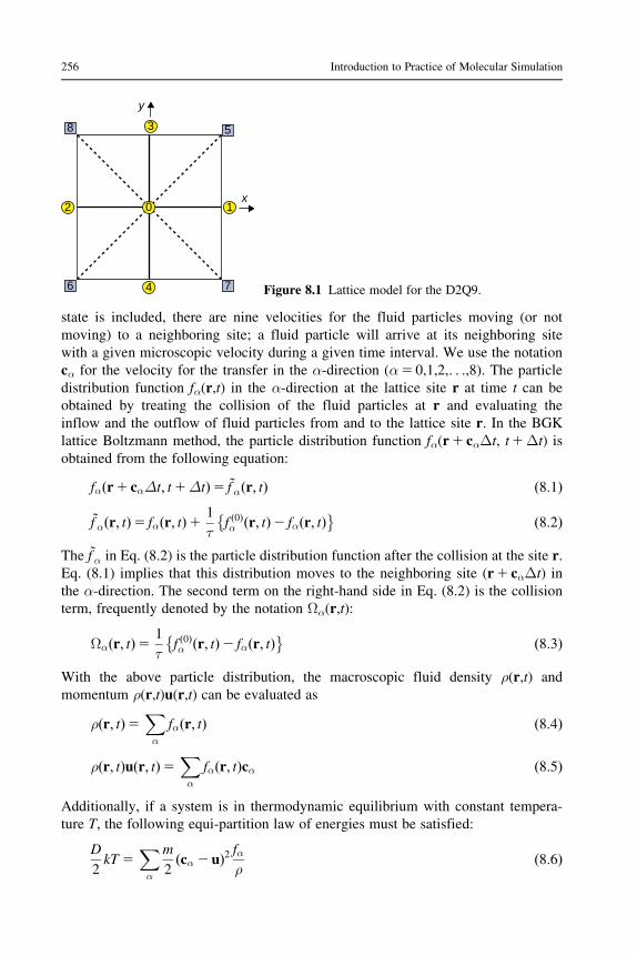
state is included, there are nine velocities for the fluid particles moving (or not
moving) to a neighboring site; a fluid particle will arrive at its neighboring site
with a given microscopic velocity during a given time interval. We use the notation
cα for the velocity for the transfer in the α-direction (α5 0,1,2,. . .,8). The particle
distribution function fα(r,t) in the α-direction at the lattice site r at time t can be
obtained by treating the collision of the fluid particles at r and evaluating the
inflow and the outflow of fluid particles from and to the lattice site r. In the BGK
lattice Boltzmann method, the particle distribution function fα(r1 cαΔt, t1Δt) is
obtained from the following equation:
fαðr1 cαΔt; t1ΔtÞ5 ~f αðr; tÞ ð8:1Þ
~f αðr; tÞ5 fαðr; tÞ11
τf ð0Þα ðr; tÞ2 fαðr; tÞ� � ð8:2Þ
The ~f α in Eq. (8.2) is the particle distribution function after the collision at the site r.
Eq. (8.1) implies that this distribution moves to the neighboring site (r1 cαΔt) in
the α-direction. The second term on the right-hand side in Eq. (8.2) is the collision
term, frequently denoted by the notation Ωα(r,t):
Ωαðr; tÞ51
τf ð0Þα ðr; tÞ2 fαðr; tÞ� � ð8:3Þ
With the above particle distribution, the macroscopic fluid density ρ(r,t) and
momentum ρ(r,t)u(r,t) can be evaluated as
ρðr; tÞ5Xα
fαðr; tÞ ð8:4Þ
ρðr; tÞuðr; tÞ5Xα
fαðr; tÞcα ð8:5Þ
Additionally, if a system is in thermodynamic equilibrium with constant tempera-
ture T, the following equi-partition law of energies must be satisfied:
D
2kT 5
Xα
m
2ðcα 2 uÞ2 fα
ρð8:6Þ
3
y
x12 0
4
8
6 7
5
Figure 8.1 Lattice model for the D2Q9.
256 Introduction to Practice of Molecular Simulation

in which D is a constant for describing the dimension with the value 2 or 3 for a
two- or three-dimensional space, respectively, and m is the mass of a fluid particle.
The thermodynamic equilibrium velocity distribution in the lattice Boltzmann
method differs from that in the MD method. This is because virtual fluid particles
in the lattice Boltzmann method are not allowed to move freely in a simula-
tion region, but are restricted to move only from site to site. The velocity c of a
molecule (a fluid particle), which moves freely in a three-dimensional space with
a uniform flow velocity u of the system, is specified by the Maxwellian distribu-
tion f (eq)(c) [25]:
f ðeqÞðcÞ5 ρm
2πkT
� �3=2
exp 2m
2kTðc2 uÞ2
n oð8:7Þ
Note that this definition includes the density ρ, whereas the usual Maxwellian dis-
tribution does not include the density in its expression. The equilibrium distribution
in the lattice Boltzmann method fα(0) may be expressed by expanding the exponen-
tial function in Eq. (8.7) in a Taylor series expansion as
f ð0Þα 5 ρwα 11 bcαUuc2
1 eu2
c21 h
ðcαUuÞ2c4
� �ð8:8Þ
in which wα, b, e, and h are unknown constants to be determined later, wα is a
weighting constant, and c is the lattice speed for fluid particles moving from site to
site, expressed as c5Δx/Δt.
In the lattice Boltzmann method, the whole system space is divided into a fine
mesh that acts as the lattice system, and the fluid particles are only able to move
from lattice site to lattice site. However, any physical phenomenon should not
depend on the setting of the lattice system, and Eqs. (8.4)�(8.6) are required to
remain valid for an arbitrary rotation of the lattice. This requirement will determine
the above-mentioned unknown constants and, because the values of these unknown
constants depend on the model used, we discuss the derivation for determining the
unknown constants for the D2Q9 and D3Q19 models separately.
8.1.1 D2Q9 Model
The xy-coordinate system and the α-direction are specified as shown in Figure 8.1.
As already pointed out, the equilibrium distribution can be obtained explicitly by
determining the unknown constants wα, b, e, and h such that the terms on the right-
hand side in Eqs. (8.4)�(8.6) remain unchanged by a rotation of the whole lattice
system by an angle φ: Before we start the procedure of determining the unknown
constants, we show preliminary expressions that are useful in the following discus-
sion. Note that the relationship of the momentum flux is necessary for determining
these constants.
257Theoretical Background of Lattice Boltzmann Method

As shown in Figure 8.2, the four unit vectors, which are along the plus and
minus x- and y-axes of the orthogonal coordinate system, are rotated about the z-
axis, and the new unit vectors are denoted by d1, d2, d3, and d4. These vectors are
written in component expressions as
d1 5 ðd1x; d1yÞ5 ðcos φ; sin φÞ
d2 5 ðd2x; d2yÞ5 cos φ1π2
0@
1A; sin φ1
π2
0@
1A
0@
1A
d3 5 ðd3x; d3yÞ5 ðcosðφ1πÞ; sinðφ1πÞÞ
d4 5 ðd4x; d4yÞ5 cos φ13π2
0@
1A; sin φ1
3π2
0@
1A
0@
1A
9>>>>>>>>>>>=>>>>>>>>>>>;
ð8:9Þ
Using these expressions, we derive several useful equations for the successive deri-
vation. Although these equations can be derived from a simple transformation, as
will be shown in the next subsection for the D3Q19 model, we here show a more
sophisticated derivation based on the concept of imaginary numbers.
With the Euler formula eiθ5 cos θ1 i sin θ for imaginary numbers, the follow-
ing relationships can be obtained:
X4k51
ðdkx1idkyÞ45X3k50
ei kπ21φð Þn o4
5X3k50
eið2πk14φÞ5ei4φX3k50
ei2πk54ei4φ ð8:10Þ
Similarly,
X4k51
ðdkx 1 idkyÞ3ðdkx 2 idkyÞ5 0
X4k51
ðdkx 1 idkyÞ2ðdkx 2 idkyÞ2 5 4
9>>>>=>>>>;
ð8:11Þ
y
d2 d1
d3 d4
xφ
Figure 8.2 Rotation of the unit vectors.
258 Introduction to Practice of Molecular Simulation

The corresponding real and imaginary parts on the left- and right-hand sides in
Eq. (8.10) are equal, which leads to the following equation:
X4k51
ðd4kx 1 d4ky 2 6d2kxd2kyÞ5 4 cos 4φ
X4k51
4ðd3kxdky 2 dkxd3kyÞ5 4 sin 4φ
9>>>>>=>>>>>;
ð8:12Þ
These relationships have been derived by expanding the left-hand side in
Eq. (8.10). Similarly, from Eq. (8.11),
X4k51
ðd4kx 2 d4kyÞ5 0
X4k51
ðd3kxdky 1 dkxd3kyÞ5 0
X4k51
ðd4kx 1 d4ky 1 2d2kxd2kyÞ5 4
9>>>>>>>>>>>=>>>>>>>>>>>;
ð8:13Þ
Further preliminary relationships can be derived from Eqs. (8.12) and (8.13).
From the first equation in Eq. (8.12) and the third equation in Eq. (8.13),
X4k51
d2kxd2ky 5
1
2ð12 cos 4φÞ ð8:14Þ
From the second equation in Eqs. (8.12) and (8.13),
X4k51
d3kxdky 51
2sin 4φ
X4k51
dkxd3ky 5 2
1
2sin 4φ
9>>>>>>=>>>>>>;
ð8:15Þ
From the first and third equations in Eq. (8.13),
X4k51
d4kx 5X4k51
d4ky 5 22X4k51
d2kxd2ky 5
3
21
1
2cos 4φ ð8:16Þ
259Theoretical Background of Lattice Boltzmann Method

From a similar derivation procedure, the terms concerning dkx or dky to the first,
second, and third powers are obtained as
X4k51
dkx 5X4k51
dky 5 0
X4k51
d2kx 5X4k51
d2ky 5 2;X4k51
dkxdky 5 0
X4k51
d3kx 5X4k51
d3ky 5X4k51
d2kxdky 5X4k51
dkxd2ky 5 0
9>>>>>>>>>=>>>>>>>>>;
ð8:17Þ
We have now obtained all the preliminary equations and will proceed to the deter-
mination procedures for the unknown constants wα, b, e, and h.
As shown in Figure 8.1, we consider the rotation of the D2Q9 lattice system
about the z-axis by the angle φ: We first evaluate the following quantity:
X8α50
wαc2αxc
2αy 5w1
X4α51
c2αxc2αy 1w5
X8α55
c2αxc2αy 5w1c
4 1
2ð12 cos 4φÞ
1w5
ffiffiffi2
pc
4 12
12 cos 4 φ1π4
n o ð8:18Þ
With the assumption of
w1 5 4w5 ð8:19Þ
Eq. (8.18) comes to be independent of φ: That is,
X8α50
wαc2αxc
2αy 5w1c
4 ð8:20Þ
Similar manipulation gives rise to
X8α50
wαc3αxcαy 5
X8α50
wαcαxc3αy 5 0
X8α50
wαc4αx 5
X8α50
wαc4αy 5 3w1c
4
9>>>>=>>>>;
ð8:21Þ
The above results can be written in one expression by using the Kronecker delta δij:X8α50
wαcαicαjcαkcαl 5w1c4ðδijδkl 1 δikδjl 1 δilδjkÞ ð8:22Þ
260 Introduction to Practice of Molecular Simulation

Similarly,
X8α50
wαcαx 5X8α50
wαcαy 5 0;X8α50
wαcαicαj 5 3w1c2δij
X8α50
wαc2αx 5
X8α50
wαc2αy 5 3w1c
2;X8α50
wαcαxcαy 5 0
X8α50
wαc3αx 5
X8α50
wαc3αy 5
X8α50
wαc2αxcαy 5
X8α50
wαcαxc2αy 5 0
9>>>>>>>>>>=>>>>>>>>>>;
ð8:23Þ
We now determine the appropriate values of the constants b, e, h, and wα for an
equilibrium distribution in Eq. (8.8). The relationships that must be satisfied for an
equilibrium state are the equation of mass in Eq. (8.4), the equation of momentum
in Eq. (8.5), and the equi-partition law of energies in Eq. (8.6). In these equations,
f ð0Þα must be used as fα. Substitution of Eq. (8.8) into the right-hand side of
Eq. (8.4) leads to
X8α50
f ð0Þα 5X8α50
ρwα 11bcαUuc2
1eu2
c21h
ðcαUuÞ2c4
� �5ρ wsum1wsum
u2
c2e13w1
u2
c2h
� �
ð8:24Þ
In deriving this equation, the following relationships have been used:
X8α50
wαðcαUuÞ5X8α50
wαðcαxux1cαyuyÞ50
X8α50
wαðcαUuÞ25X8α50
wαðc2αxu2x1c2αyu2y12uxuycαxcαyÞ53w1c
2u2
9>>>>>=>>>>>;
ð8:25Þ
Equation (8.4) says that the quantity in Eq. (8.24) must equal the density ρ, so that
the following relationships are obtained:
wsum 5 1; wsume1 3w1h5 0 ð8:26Þ
in which wsum5w01 4w11 4w55w01 5w1.
Similarly, we obtain the following equation:
X8α50
cαifð0Þα 5
X8α50
ρwαcαi 11 bcαUuc2
1 eu2
c21 h
ðcαUuÞ2c4
� �5 3ρw1uib ð8:27Þ
in which the following relationships have been used for the derivation.
261Theoretical Background of Lattice Boltzmann Method

X8α50
wαcαxðcαUuÞ5X8α50
wαðc2αxux 1 cαxcαyuyÞ5 3w1c2ux
X8α50
wαcαxðcαUuÞ2 5X8α50
wαðc3αxu2x 1 2c2αxcαyuxuy 1 cαxc2αyu
2yÞ5 0
9>>>>=>>>>;
ð8:28Þ
Since the momentum equation in Eq. (8.5) must be satisfied, b is obtained as
b51
3w1
ð8:29Þ
Then, we evaluate the momentum flux Πð0Þij by substituting the equilibrium dis-
tribution f ð0Þα in Eq. (8.8) into this momentum flux expression:
Πð0Þij 5
X8α50
cαicαj fð0Þα 5
X8α50
ρwαcαicαj 11 bcαUuc2
1 eu2
c21 h
ðcαUuÞ2c4
8<:
9=;
5 ρw1 3c2 11u2
c2e
0@
1Aδij 1 u2hδij
8<:
9=;1 2ρw1uiujh
ð8:30Þ
in which the following relationships have been used for deriving this equation:
X8α50
wαcαxcαyðcαUuÞ5X8α50
wαc2αxðcαUuÞ5
X8α50
wαc2αyðcαUuÞ5 0
X8α50
wαcαxcαyðcαUuÞ2 5 2w1c4uxuy
X8α50
wαc2αxðcαUuÞ2 5 2w1c
4u2x 1w1c4u2
9>>>>>>>>>=>>>>>>>>>;
ð8:31Þ
For the case of an equilibrium state, Πð0Þij can be related to the pressure p as
Πð0Þij 5 pδij 1 ρuiuj ð8:32Þ
Hence, the comparison of Eq. (8.30) with Eq. (8.32) yields the following
relationships:
h51
2w1
; p5 3ρw1c2 ð8:33Þ
3e1 h5 0 ð8:34Þ
262 Introduction to Practice of Molecular Simulation

The pressure p is related to the speed of sound cs as p5 ρc2s ; so that cs can be
written as
cs 5ffiffiffiffiffiffiffiffi3w1
pc ð8:35Þ
Finally, we evaluate the kinetic energy. Preliminary relationships can be derived
from Eq. (8.23) as
X8α50
wαc2α 5 6w1c
2
X8α50
wαc2αxðcαUuÞ5
X8α50
wαc2αyðcαUuÞ5
X8α50
wαc2αðcαUuÞ5 0
X8α50
wαc2αðcαUuÞ2 5 4w1c
4u2;X8α50
wαðcαUuÞ3 5 0
9>>>>>>>>>=>>>>>>>>>;
ð8:36Þ
Using these relationships, the right-hand side in Eq. (8.6) may be calculated as
X8α50
m
2ðcα 2 uÞ2 fα
ð0Þ
ρ5
m
2
X8α50
wαðcα2 1 u2 2 2cαUuÞ
3 11 bcαUuc2
1 eu2
c21 h
ðcαUuÞ2c4
� �
5m
26w1 11 e
u2
c2
� �c2 1 4w1hu
2 1wsum 11 eu2
c2
� �u2 1 3w1h
u4
c22 6w1bu
2
� �ð8:37Þ
By taking into account Eqs. (8.26), (8.29), and (8.33), the above equation is simpli-
fied as
X8α50
m
2ðcα 2 uÞ2 fα
ð0Þ
ρ5
m
2ð6w1c
2 1 6w1u2e1wsumu
2Þ ð8:38Þ
Hence, Eq. (8.6) reduces to
2
2kT 5
m
2ð6w1c
2 1 6w1u2e1wsumu
2Þ ð8:39Þ
Since the temperature T is independent of the macroscopic velocity u, this equation
yields the final relationships:
6w1e1wsum 5 0 ð8:40Þ
3mw1c2 5 kT ð8:41Þ
263Theoretical Background of Lattice Boltzmann Method

We now have the same number of equations as the unknown constants, so that the
solutions required can be obtained in a straightforward way as
b5 3; e5 23
2; h5
9
2ð8:42Þ
wsum 5 1; w0 54
9; w1 5
1
9; w5 5
1
36ð8:43Þ
We summarize the final results as
f ð0Þα 5 ρwα 11 3cαUuc2
23
2Uu2
c21
9
2UðcαUuÞ2
c4
� �ð8:44Þ
wα 5
4=9 for α5 0
1=9 for α5 1; 2; 3; 4
1=36 for α5 5; 6; 7; 8
; cαj j50 for α5 0
c for α5 1; 2; 3; 4ffiffiffi2
pc for α5 5; 6; 7; 8
8><>:
8><>:
ð8:45Þ
The speed of sound cs is expressed as
cs 5 c=ffiffiffi3
pð8:46Þ
8.1.2 D3Q19 Model
In the case of the D3Q19 lattice model, the thermodynamic equilibrium distribution
can be assumed to have the form of Eq. (8.8), and therefore the unknown constants
can be derived through similar procedures to the previous D2Q9 model. Only in
this present subsection, we use the notation ~cð5Δx=ΔtÞ for the lattice speed
instead of c, since the notation c will be used for the abbreviated symbol of the
cosine function.
In order to satisfy the isotropy condition, the lattice system has to be adopted
such that it is independent of an arbitrary rotation of the lattice. In Figure 8.3, for a
rotation of the lattice system about the z-axis by an angle φ and a rotation about
the y-axis by an angle θ, the rotation matrix R is written as
R5cos θ 0 sin θ0 1 0
2sin θ 0 cos θ
0@
1A cos φ 2sin φ 0
sin φ cos φ 0
0 0 1
0@
1A5
Cc 2Cs S
s c 0
2Sc Ss C
0@
1Að8:47Þ
264 Introduction to Practice of Molecular Simulation

in which the abbreviations C5 cos θ, S5 sin θ, c5 cos φ, and s5 sin φ are used
for simplification of the equations. An arbitrary component X is related to the
corresponding rotated component X0 by the expression X0 5R �X. The transferred
component dk (k5 1,2,. . .,18) of each lattice point in Figure 8.3 is obtained as
d1 5R
1
0
0
0B@
1CA5
Cc
s
2Sc
0B@
1CA; d3 5R
0
1
0
0B@
1CA5
2Cs
c
Ss
0B@
1CA; d5 5
2S
0
2C
0B@
1CA
d7 5
C c2 sð Þs1 c
2S c2 sð Þ
0B@
1CA; d9 5
C c1 sð Þs2 c
2S c1 sð Þ
0B@
1CA; d11 5
2Cs1 S
c
Ss1C
0B@
1CA
d13 5
Cs1 S
2c
2Ss1C
0B@
1CA; d15 5
Cc1 S
s
2Sc1C
0B@
1CA; d17 5
Cc2 S
s
2Sc2C
0B@
1CA
9>>>>>>>>>>>>>>>>>=>>>>>>>>>>>>>>>>>;
ð8:48Þ
From symmetric considerations, the following relationship must be satisfied:
d2k 5 2d2k2 1 ðk51; 2; . . . ; 9Þ ð8:49Þ
The final expressions are summarized in Table 8.1.
The results in Table 8.1 give rise to those concerning cαx, cαy, and cαz, such asP18α50
5wαcαicαjcαkcαl in Table 8.2. As seen from the result ofP18α50
wαc4αi; the
z
x
y
6
2
4
5
1
3 7
9
10
8
18
1716
1511
13
14
12
0
Figure 8.3 Lattice model for the
D3Q19.
265Theoretical Background of Lattice Boltzmann Method

Table 8.1 Results of Quantities for the Successive Derivation
X6k51
d4kx 5 24ðC2S2 1C4c2s2Þ1 2
X6k51
d4ky 5 4ðc4 2 c2Þ1 2
X6k51
d4kz 5 24ðC2S2 1 S4c2s2Þ1 2
X18k57
d4kx 5 8ðC2S2 1C4c2s2Þ1 8
X18k57
d4ky 5 2 8ðc4 2 c2Þ1 8
X18k57
d4kz 5 8ðC2S2 1 S4c2s2Þ1 8
X6k51
d2kxd2ky 5 4C2c2s2
X6k51
d2kxd2kz 5 4C2S2ð12 c2s2Þ
X6k51
d2kyd2kz 5 4S2c2s2
X18k57
d2kxd2ky 5 28C2c2s2 1 4
X18k57
d2kxd2kz 5 28C2S2ð12 c2s2Þ1 4
X18k57
d2kyd2kz 5 28S2c2s2 1 4
X6k51
d2kxdkydkz 5 2C2Scsð2c2 1 s2ÞX6k51
dkxd2kydkz 5 24CSc2s2
X6k51
dkxdkyd2kz 5 2CS2csðc2 2 s2Þ
X18k57
d2kxdkydkz 5 4C2Sðc2 2 s2ÞcsX18k57
dkxd2kydkz 5 8CSc2s2
X18k57
dkxdkyd2kz 5 24CS2ðc2 2 s2Þcs
X6k51
d3kxdky 5 2C3csðc2 2 s2ÞX6k51
d3kxdkz 5 22C3Sð12 2c2s2Þ1 2CS3
X6k51
d3kydkx 5 2Ccsð2c2 1 s2ÞX6k51
d3kydkz 5 2Scsðc2 2 s2ÞX6k51
d3kzdkx 5 22CS3ð12 2c2s2Þ1 2C3S
X6k51
d3kzdky 5 22S3csðc2 2 s2Þ
X18k57
d3kxdky 5 24C3ðc2 2 s2ÞcsX18k57
d3kxdkz 5 4C3Sð12 2c2s2Þ2 4CS3
X18k57
d3kydkx 5 4Cðc2 2 s2ÞcsX18k57
d3kydkz 5 24Sðc2 2 s2ÞcsX18k57
d3kzdkx 5 4CS3ð12 2c2s2Þ2 4C3S
X18k57
d3kzdky 5 4S3ðc2 2 s2ÞcsX6k51
d2kx 5X6k51
d2ky 5X6k51
d2kz 5 2
X6k51
dkxdky 5X6k51
dkxdkz 5X6k51
dkydkz 5 0
X18k57
d2kx 5X18k57
d2ky 5X18k57
d2kz 5 8
X18k57
dkxdky 5X18k57
dkxdkz 5X18k57
dkydkz 5 0
266 Introduction to Practice of Molecular Simulation

Table 8.2 Final Results of Quantities for the Successive Derivation
X18α50
wαc4αx 5 ~c4ð2 4w1 1 8w7ÞðC2S2 1C4c2s2Þ1 ~c4ð2w1 1 8w7Þ
X18α50
wαc4αy 5 ~c4ð4w1 2 8w7Þðc4 2 c2Þ1 ~c4ð2w1 1 8w7Þ
X18α50
wαc4αz 5 ~c4ð2 4w1 1 8w7ÞðC2S2 1 S4c2s2Þ1 ~c4ð2w1 1 8w7Þ
+ w1 5 2w7
X18α50
wαc4αx 5
X18α50
wαc4αy 5
X18α50
wαc4αz 5 6w1 ~c
4
X18α50
wαc2αxc
2αy5
X18α50
wαc2αxc
2αz5
X18α50
wαc2αyc
2αz52w1 ~c
4
X18α50
wαc3αxcαy5
X18α50
wαc3αxcαz5
X18α50
wαc3αycαx5
X18α50
wαc3αycαz5
X18α50
wαc3αzcαx5
X18α50
wαc3αzcαy50
X18α50
wαc2αxcαycαz5
X18α50
wαcαxc2αycαz5
X18α50
wαcαxcαyc2αz50
X18α50
wαc3αx5
X18α50
wαc3αy5
X18α50
wαc3αz50
X18α50
wαc2αxcαy5
X18α50
wαc2αxcαz5
X18α50
wαc2αycαx5
X18α50
wαc2αycαz5
X18α50
wαc2αzcαx5
X18α50
wαc2αzcαy50
X18α50
wαcαxcαycαz50
X18α50
wαc2αx 5
X18α50
wαc2αy 5
X18α50
wαc2αz 5 6w1 ~c
2
X18α50
wαcαxcαy 5X18α50
wαcαxcαz 5X18α50
wαcαycαz 5 0
X18α50
wαcαx 5X18α50
wαcαy 5X18α50
wαcαz 5 0
267Theoretical Background of Lattice Boltzmann Method

relationship of w15 2w7 has to be satisfied in order for this result to be independent
of the rotational angle. Hence, the results after the arrow in Table 8.2 have taken
into account this relationship. The expressions in Table 8.2 are written in simply
unified equations as
X18α50
wαcαicαjcαkcαl 5 2w1 ~c4ðδijδkl 1 δikδjl 1 δilδjkÞ
X18α50
wαcαicαjcαk 5 0
X18α50
wαcαicαj 5 6w1 ~c2δij;
X18α50
wαci 5 0
9>>>>>>>>>=>>>>>>>>>;
ð8:50Þ
We are now ready to derive the equilibrium distribution for the D3Q19 lattice
model.
As mentioned before, the relationships that the equilibrium distribution f ð0Þαshown in Eq. (8.8) must satisfy are the mass, momentum, kinetic energy, and
momentum flux equations. The former three equations are written as
X18α50
f ð0Þα 5 ρ ð8:51Þ
X18α50
cαfð0Þα 5 ρu ð8:52Þ
X18α50
m
2ðcα 2 uÞ2 f ð0Þα
ρ5
3
2kT ð8:53Þ
With the results shown in Table 8.2, the following equation is obtained:
X18α50
f ð0Þα 5X18α50
wαρ 11 bcαUu
~c21 e
u2
~c21 h
ðcαUuÞ2~c4
� �
5 ρ wsum 1u2
~c2ðwsume1 6w1hÞ
� �ð8:54Þ
The comparison of this equation with Eq. (8.51) leads to
wsum 5 1; wsume1 6w1h5 0 ð8:55Þ
in which wsum5w01 6w11 12w75w01 12w1.
268 Introduction to Practice of Molecular Simulation

In order to compare this result with the right-hand side of Eq. (8.52), the left-
hand side is evaluated using the equilibrium distribution as
X18α50
cαifð0Þα 5
X18α50
ρwαcαi 11 bcαUu
~c21 e
u2
~c21 h
ðcαUuÞ2~c4
� �5 6bw1ρui ð8:56Þ
Hence, the comparison of the right-hand sides in Eqs. (8.56) and (8.52) gives rise
to
6w1b5 1 ð8:57Þ
Similar to the D2Q9 model, the momentum flux Πð0Þij is calculated as
Πð0Þij 5
X18α50
cαicαj fð0Þα 5 6ρw1 ~c
2 11 eu2
~c2
� �1 2ρw1u
2h
� �δij 1 4ρw1uiujh
ð8:58Þ
In deriving this equation, the following relationships are used:
X18α50
wαcαxcαy 11 bcαUu
~c21 e
u2
~c21 h
ðcαUuÞ2~c4
8<:
9=;5 4w1uxuyh
X18α50
wαc2αx 11 b
cαUu
~c21 e
u2
~c21 h
ðcαUuÞ2~c4
8<:
9=;
5 6w1 ~c2 11 e
u2
~c2
0@
1A1 2w1u
2h1 4w1u2xh
9>>>>>>>>>>>>>>>=>>>>>>>>>>>>>>>;
ð8:59Þ
The expression for Πð0Þij as defined by Eq. (8.32) is also valid for a three-dimen-
sional system. The following relationships can therefore be obtained by comparison
with Eq. (8.58) as
p5 6ρw1 ~c2 ð8:60Þ
4w1h5 1; 3e1 h5 0 ð8:61Þ
Hence, the speed of sound cs is expressed from p5 ρc2s as
cs 5ffiffiffiffiffiffiffiffi6w1
pU ~c ð8:62Þ
269Theoretical Background of Lattice Boltzmann Method

Finally, in order to compare with Eq. (8.53), the following reformation is
performed:
X18α50
ðcα2uÞ2 fð0Þα
ρ5X18α50
wαðcα2uÞ2 11bcαUu
~c21e
u2
~c21h
ðcαUuÞ2~c4
8<:
9=;
5X18α50
wαðc2α22cαUu1u2Þ 11bcαUu
~c21e
u2
~c21h
ðcαUuÞ2~c4
8<:
9=;
5X18α50
wαðc2α22cαUu1u2Þ 11eu2
~c2
0@
1A
1X18α50
wαðc2α22cαUu1u2ÞðcαUuÞ b~c2
1X18α50
wαðc2α22cαUu1u2ÞðcαUuÞ2 h~c4
5 11eu2
~c2
0@
1Að18w1 ~c
21wsumu2Þ2 2b
~c2X18α50
wαðcαUuÞ2
1h
~c4X18α50
wα
(c2αðcαUuÞ21u2ðcαUuÞ2
)
518w1 ~c21 ðwsum212w1b118w1e110w1hÞu2 ð8:63Þ
in which Eq. (8.55) and the following relationship have been used for the
derivation:
X18α50
wαðcαUuÞ2 5 6w1 ~c2u2
X18α50
wαc2αðcαUuÞ2 5 10w1 ~c
4u2
9>>>>=>>>>;
ð8:64Þ
Since the temperature is independent of the macroscopic velocity u, the second
term on the right-hand side in Eq. (8.63) must vanish:
wsum 2 12w1b1 18w1e1 10w1h5 0 ð8:65Þ
The comparison of Eq. (8.63) with Eq. (8.6) yields the following equation:
m
218w1 ~c
2 53
2kT ð8:66Þ
270 Introduction to Practice of Molecular Simulation

We now have the same number of equations as the unknown constants. The final
results for the unknown constants can be obtained from Eqs. (8.55), (8.57), (8.61),
and (8.65) and the relationships of w15 2w7 and wsum5w01 12w1, as
w0 51
3; w1 5
1
18; w7 5
1
36; wsum 5 1
b5 3; e5 23
2; h5
9
2
9>>>=>>>;
ð8:67Þ
With the original notation c for the lattice velocity, the equilibrium distribution for
the D3Q19 model is finally written as
f ð0Þa 5 ρwα 11 3cαUuc2
23
2Uu2
c21
9
2UðcαUuÞ2
c4
� �ð8:68Þ
wα 51=3 for α50
1=18 for α5 1; 2; . . . ; 61=36 for α5 7; 8; . . . ; 18
; cαj j50 for α5 0
c for α5 1; 2; . . . ; 6ffiffiffi2
pc for α5 7; 8; . . . ; 18
8<:
8<:
ð8:69Þ
8.2 Navier�Stokes Equation
In this section, we derive the Navier�Stokes equation from the preliminary equa-
tions derived in Appendix A1, which is the basic macroscopic equation for flow
problems. The following derivation procedure is valid for both D2Q9 and D3Q19
models, with the exception that α is taken as α5 0,1,. . .,8, the axis index i is x or y
for the former model, α is taken as α5 0,1,. . .,18, and i is x, y, or z for the latter
model.
The starting equation for the derivation procedure is Eq. (A1.27), rewritten as
@
@tðρuiÞ1
Xj
@
@rjΠij1
Δt
2εXj
@
@rj
@
@t1Πð0Þ
ij
� �1
Δt
2
Xj
Xk
@
@rj
@
@rkSð0Þijk
� �50
ð8:70Þ
Another starting equation is Eq. (A1.31), rewritten as
21
τΔtf ð1Þα 52
@f ð0Þα
@ρU
@
@r1UðρuÞ2
Xi
Xj
@f ð0Þα
@ðρuiÞU
@
@r1jΠð0Þ
ij 1Xi
@
@r1iðcαif ð0Þα Þ
ð8:71Þ
271Theoretical Background of Lattice Boltzmann Method

in which
fα 5 f ð0Þα 1 εf ð1Þα 1 ε2f ð2Þα 1? ð8:72Þ
Πð0Þij 5
Xα
cαicαj fð0Þα 5 pδij 1 ρuiuj 5
ρ3c2δij 1 ρuiuj ð8:73Þ
Sð0Þijk 5
Xα
cαicαjcαkfð0Þα ð8:74Þ
@
@t5 ε
@
@t11 ε2
@
@t2;
@
@ri5 ε
@
@r1ið8:75Þ
We now begin the derivation procedure for the Navier�Stokes equation by
deriving the solution for f ð1Þα from the basic equation in Eq. (8.71). If the terms
higher than the order of (u/c)2 are neglected, the following relationships are
obtained:
f ð0Þα 5 ρwα 11 3cαUuc2
n oð8:76Þ
Πð0Þij 5
ρ3c2δij 1 ρuiuj ð8:77Þ
@f ð0Þα
@ρ5wα ð8:78Þ
@f ð0Þα
@ðρuiÞ5wα
@
@ðρuiÞ3
c2
Xj
cαjðρujÞ( )
5wα3
c2cαi ð8:79Þ
@
@r1jΠð0Þ
ij 5c2
3U@ρ@r1j
δij 1@
@r1jðρuiujÞ ð8:80Þ
@
@r1iðcαif ð0Þα Þ5wα
@
@r1iðρcαiÞ1 3wα
1
c2U
@
@r1i
Xj
ρcαicαjuj
( )ð8:81Þ
By substituting these relationships into Eq. (8.71), the solution of f ð1Þα can finally be
obtained as
f ð1Þα 523wαΔtτ1
c2
Xk
Xl
cαkcαl21
3c2δkl
� �@
@r1lðρukÞ ð8:82Þ
272 Introduction to Practice of Molecular Simulation

With this solution, the next quantity can be evaluated:
εΠð1Þij 5 ε
Xα
cαicαj fð1Þα
523Δtτ1
c2
Xk
Xl
Xα
wαcαicαjcαkcαl
!@
@rlðρukÞ
1ΔtτPαwαcαicαj
@
@rUðρuÞ
52Δtτc2
3
@
@rjðρuiÞ1
@
@riðρujÞ
8<:
9=;
ð8:83Þ
In deriving this equation, Eqs. (8.50), (8.22), and (8.23) are used. This equation
leads to
Xj
@
@rjðεΠð1Þ
ij Þ52Δtτc2
3
@2
@r2ðρuiÞ1
@
@ri
@
@rUðρuÞ
� �� �ð8:84Þ
On the other hand, Πð0Þij is written as
Xj
@
@rjðΠð0Þ
ij Þ5Xj
@
@rjðpδij 1 ρuiujÞ ð8:85Þ
With the approximation of Πij � Πð0Þij 1 εΠð1Þ
ij ; the following equation is obtained
from Eqs. (8.84) and (8.85):
Xj
@
@rjΠij5
Xj
@
@rjðpδij1ρuiujÞ2
Δtτc2
3
@2
@r2ðρuiÞ1
@
@ri
@
@rUðρuÞ
� �� �ð8:86Þ
Moreover, Eqs. (A1.11) and (A1.17) give rise to
Δt
2ε@
@t1Πð0Þ
ij 51
6Δtc2δijε
@ρ@t1
521
6Δtc2δij
@
@rUðρuÞ ð8:87Þ
From this equation, the following equation can be obtained:
Δt
2εXj
@
@rj
@
@t1Πð0Þ
ij
� �5 2
1
6Δtc2
@
@ri
@
@rUðρuÞ
� �ð8:88Þ
We next evaluate the quantity Sð0Þijk : First,
Sð0Þijk 5
Xα
cαicαjcαk fð0Þα 5
Xα
wαcαicαjcαkρ 11 3cαUuc2
ð8:89Þ
273Theoretical Background of Lattice Boltzmann Method

With this equation, the partial derivative in Eq. (8.70) is obtained as
Xj
Xk
@
@rjU
@
@rkSð0Þijk
5
1
3c2Xj
Xk
@
@rjU
@
@rkðρukδij 1 ρujδik 1 ρuiδjkÞ
52
3c2
@
@ri
@
@rUðρuÞ
� �1
1
2U@2
@r2ðρuiÞ
� �ð8:90Þ
We have now finished the preparation for deriving the Navier�Stokes equation.
If the summation of the first and second terms, and the summation of the third and
fourth terms on the left-hand side in Eq. (8.70), are denoted by A and B, respec-
tively, these quantities are evaluated as
A5@
@tðρuiÞ1
Xj
@
@rjðpδij 1 ρuiujÞ2
Δtτc2
3
@2
@r2ðρuiÞ1
@
@ri
@
@rUðρuÞ
0@
1A
8<:
9=;
5@
@tðρuiÞ1
Xj
@
@rjðρuiujÞ1
@p
@ri2
Δtτc2
3
@2
@r2ðρuiÞ1
@
@ri
@
@rUðρuÞ
0@
1A
8<:
9=;
ð8:91Þ
B5Δt
2εXj
@
@rj
@
@t1Πð0Þ
ij
0@
1A1
Δt
2
Xj
Xk
@
@rj
@
@rkSð0Þijk
0@
1A
51
6Δtc2
@2
@r2ðρuiÞ1
@
@ri
@
@rUðρuÞ
0@
1A
8<:
9=;
ð8:92Þ
By substituting Eqs. (8.91) and (8.92) into Eq. (8.70), together with the relationship
of @@r UðρuÞ5 0 for noncompressible fluids, the Navier�Stokes equation is finally
obtained as
ρ@u
@t1 ðuUrÞu
� �5 2rp1μLBr2u ð8:93Þ
in which μLB is the viscosity, expressed as
μLB 5ρΔtc2
3τ2
1
2
� �; νLB 5
μLB
ρ5
Δtc2
3τ2
1
2
� �ð8:94Þ
In this equation vLB is the kinematic viscosity.
274 Introduction to Practice of Molecular Simulation

8.3 Body Force
If a body force, such as the gravitational force, acts on a fluid, how do we incorpo-
rate it into the lattice Boltzmann equation? The method can be seen in the
following:
fαðr1 cαΔt; t1ΔtÞ5 ~f αðr; tÞ~f αðr; tÞ5 fαðr; tÞ1Ωα 1 gα
9=; ð8:95Þ
in which
Ωα 51
τf ð0Þα ðr; tÞ2 fαðr; tÞ� � ð8:96Þ
gα 5
0 for α5 0
3Δt
c2wαcαUF for α 6¼ 0
8><>:
9>=>; ð8:97Þ
gα is a quantity that is due to the body force F per unit volume and has the follow-
ing characteristics:
Xα
gα 5 0
Xα
cαgα 5Xα
3Δt
c2wαðcαcαÞUF5ΔtF
9>>>=>>>;
ð8:98Þ
In this reformation, the following relationship has been used:
Xα
wαcαcα 5 ðc2=3ÞI ð8:99Þ
in which I is the unit tensor, and Eq. (8.99) is valid for both D2Q9 and D3Q19
models. It is quite clear that the quantity gα can be expressed in the form of
Eq. (8.97), because the particle distribution tends to move in the direction of the
body force F acting. Therefore, the relationship of the form gα~cα �F can be
expected.
We will now confirm that the gα, expressed in Eq. (8.97), appears in a reason-
able form in the Navier�Stokes equation by deriving these equations starting from
Eq. (8.95), as conducted in Section 8.2. There is no new concept applied here
except for the inclusion of the new term gα into the derivation procedure shown in
Section 8.2; therefore we show only the important expressions.
275Theoretical Background of Lattice Boltzmann Method

From Appendix A1, the relationships of the orders ε and ε2 are written as
@ρ@t1
1r1UðρuÞ5 0
@
@t1ðρuiÞ1
Xj
@
@r1jΠð0Þ
ij 51
εFi
@ρ@t2
1Δt
2U@2ρ@t21
1Δt
2
Xi
Xj
@
@r1iU
@
@r1jΠð0Þ
ij 1ΔtXi
@
@t1U
@
@r1iðρuiÞ5 0
9>>>>>>>>>>=>>>>>>>>>>;ð8:100Þ
@
@t2ðρuiÞ1
Δt
2U@2
@t21ðρuiÞ1
Xj
@
@r1jΠð1Þ
ij 1Δt
2
Xj
Xk
@
@r1jU
@
@r1kSð0Þijk
1ΔtXj
@
@t1U
@
@r1jΠð0Þ
ij 5 0
ð8:101Þ
These expressions lead to the following basic equations:
@ρ@t
1rUðρuÞ5 0 ð8:102Þ
@
@tðρuiÞ1
Xj
@
@rjΠij 1
Xj
Δt
2U@
@rjε@
@t1Πð0Þ
ij 1Xk
@
@rkSð0Þijk
( )5Fi ð8:103Þ
Also, f ð1Þα is written as
f ð1Þα 52 tτΔt@f ð0Þα
@t11Xi
@
@r1icαif
ð0Þα
� �8<:
9=;1
τεgα
523wαΔtτ1
c2
Xk
Xl
cαkcαl 21
3c2δkl
0@
1A @
@r1lðρukÞ
ð8:104Þ
Finally, using these expressions in a derivation procedure similar to that used previ-
ously, the Navier�Stokes equation is obtained as
ρ@u
@t1 ðuUrÞu
� �52rp1μLBr2u1F ð8:105Þ
in which μLB has already been shown in Eq. (8.94). Eq. (8.105) clearly shows that
gα defined in Eq. (8.97) gives rise to the body force F appearing in the appropriate
form in the Navier�Stokes equation.
276 Introduction to Practice of Molecular Simulation

8.4 Boundary Conditions
In simulations by the lattice Boltzmann method, it is very important to treat the
boundary conditions in an appropriate manner at all the simulation boundary sur-
faces. Hence, there is a lot of current interest in developing more accurate boundary
conditions, and papers addressing this problem have been appearing in academic
journals. For example, if we consider a flow inside a tube or around an obstacle, or
a suspension composed of solid particles, the treatment of the boundary condition
at the wall or particle surface is very important for obtaining reliable solutions of
the flow field. In this section, we first explain the historical bounce-back boundary
condition, and then focus on several alternative boundary conditions that have a
clearer physical and mathematical background.
8.4.1 Bounce-back Rule
We explain the historical bounce-back rule [35,36] using Figure 8.4. The lattice
position of interest in a fluid is denoted by rl, its neighboring site inside the mate-
rial by rp, and the point at the material surface on a straight line between these two
points by rw, as shown in Figure 8.4. According to the BGK lattice Boltzmann
method, the particle distribution ~f α after the collision at time t becomes that at the
neighboring site in the α-direction at time (t1Δt). The bounce-back rule employs
the following treatment of the collision at the material surface:
fαðrl; t1ΔtÞ5 ~f αðrl; tÞ2 2ρwαuwUcαc2s
ð8:106Þ
fαðrp; t1ΔtÞ5 ~f αðrp; tÞ1 2ρwαuwUcαc2s
ð8:107Þ
r l
rw
rp
Figure 8.4 Bounce-back rule for the treatment at
the material surface.
277Theoretical Background of Lattice Boltzmann Method

in which α implies the opposite direction of α; α is the direction toward the object.
Eq. (8.106) means that the fluid particles at r5 rl move in the α-direction, collidewith the obstacle at the middle point of the two lattice points, and return to the
original lattice point during t and t1Δt. In this movement, if the solid surface
moves in the α-direction, the number of the particles returning after the collision
decreases, so that the second term on the right-hand side in Eq. (8.106) is necessary
to make this modification. The following consideration makes clear that the
bounce-back rule does not offer sufficient accuracy. That is, in the treatment of
Eq. (8.106), the fluid particles starting from the point rl do not collide with the
actual solid surface rw, but at the exact middle point between rl and rp, beforereturning to the original site. In other words, the collision procedure is conducted
under the assumption that the surface of the obstacle is at the middle point between
two neighboring lattice sites. In order to improve this approach, various boundary
conditions have been developed. Research in this area is still a topic of interest.
Here we consider the validity of the second term on the right-hand side in
Eq. (8.106). The consideration of Eqs. (8.82), (8.72), and (A1.11) leads to
~f αðrl; tÞ5 fαðrl; tÞ11
τf ð0Þα ðrl; tÞ2 fαðrl; tÞ� �
5 fαðrl; tÞ1ρwα
c2scαU
@uðrlÞ@r
� �UcαΔt
ð8:108Þ
in which a fluid has been assumed to be noncompressive. Substituting this equation
into Eq. (8.106) yields
fαðrl; t1ΔtÞ5 fαðrl; tÞ1 ρwα
c2scαU
@uðrlÞ@r
� �UcαΔt2 2ρwα
uwUcαc2s
ð8:109Þ
If fα(rl,t) in Eq. (8.109) is assumed to be not far from an equilibrium state, it is
approximated from Eq. (8.68) as
fαðrl; tÞ � fαðrl; tÞ1 2ρwαuðrlÞUcα
c2sð8:110Þ
Substituting this equation into Eq. (8.109) gives rise to
fαðrl;t1ΔtÞ5fαðrl; tÞ12ρwα
c2suðrlÞ1 @uðrlÞ
@rUΔt
2cα
� �2uw
�Ucα
� fαðrl; tÞ12ρwα
c2suðrl1cαΔt=2Þ2uw� �
Ucα
ð8:111Þ
It is seen from Eq. (8.111) that u(rl1 (1/2)cαΔt) is equal to uw, if the medium point
(rl1 (1/2)cαΔt) is sufficiently near to the solid surface. Hence, we obtain the result
fαðrl; t1ΔtÞ5 fαðrl; tÞ: That is, the particle distribution in the direction away from
278 Introduction to Practice of Molecular Simulation

the solid surface approximates to the equilibrium distribution and is independent
of time.
8.4.2 BFL Method
In this subsection we explain the BFL method [37]. In the bounce-back rule, the
solid surface is regarded as being at the middle point of two lattice sites, and virtual
fluid particles are reflected at this point. Hence, the exact position of the solid sur-
face is not employed in the bounce-back method. The BFL method attempts to
improve this drawback by taking into account the exact position of the solid surface
in the procedure of the collision process between virtual fluid particles and the
material. As shown in Figure 8.5, rl is the point of interest in a fluid, rp is the neigh-
boring point inside the particle, rw is the point at the solid surface on a line between
these two points, and rl0 is the next neighboring point in the direction away from the
solid surface. The exact position of the solid surface can be expressed using the
quantity Δw5 jrl2 rwj/jrl2 rpj; although the lattice separation is defined to be Δx,
we regarded Δx as unity in Sections 8.4.2 and 8.4.3 for simplicity’s sake, because
the final results derived here are unaffected even if Δx is not unity. The solid sur-
face is at the position which is away from rl in the direction toward rp determined
by Δw, as shown in Figure 8.5. The BFL method is based on an interpolation but,
so as not to lose the accuracy of the interpolation, two different procedures are
adopted for Δw# 1/2 and Δw. 1/2, although the concept of the treatment is the
same for both cases. The fundamental concept is that fluid particles move, collide
with the solid material, and return to a certain point during the time interval Δt.
Since the unit lattice length is assumed in this analysis, the transportation distance is
unity. In this collision process, the exact position of the solid surface is necessary.
In the following text, the treatment for Δw# 1/2 is discussed first.
As shown in Figure 8.5A, in the case of Δw# 1/2, the particle distribution func-
tion ~f αðrm; tÞ at rm becomes that at rl, fαðrl; t1ΔtÞ; in which the point rm is evalu-
ated such that fluid particles move in the α-direction, collide with the solid surface,
and arrive at the lattice point rl; the distance of travel for a fluid particle is just
unity. The point rm can be obtained straightforwardly as the position away from rl
r l″(A) (B)
r l ′ r l rp
rwrm
1–2Δw Δw
r l″ r l ′ r l rp
rw
rm
2Δw –1 1–Δw
Figure 8.5 BFL method for the treatment at the material surface.
279Theoretical Background of Lattice Boltzmann Method

at the distance of (12 2Δw), shown in Figure 8.5A. Hence, the particle distribution
function ~f αðrm; tÞ is easily obtained from the quadratic extrapolation procedure as
~f αðrm; tÞ5Δwð11 2ΔwÞ ~f αðrl; tÞ1 ð12 4Δ2wÞ ~f αðrl0 ; tÞ2Δwð12 2ΔwÞ ~f αðrlv; tÞ
ð8:112Þ
Since fluid particles collide with the solid surface, fαðrl; t1ΔtÞ can finally be
obtained as
fαðrl; t1ΔtÞ5 ~f αðrm; tÞ2 2ρwαuwUcαc2s
ð8:113Þ
Equation (8.112) has been obtained from the following formula of the quadratic
interpolation method. If an arbitrary function h(x) has values h(x1), h(x2), and h(x3)
for x5 x1, x2, and x3, respectively, h(x) at an arbitrary position x between x1 and x3can be given from the quadratic interpolation as
hðxÞ5 ðx2x2Þðx2x3Þðx12x2Þðx12x3Þ
hðx1Þ1ðx2x1Þðx2x3Þðx22x1Þðx22x3Þ
hðx2Þ1ðx2x1Þðx2x2Þðx32x1Þðx32x2Þ
hðx3Þ
ð8:114Þ
We now consider the treatment for Δw. 1/2. As shown in Figure 8.5B, fluid
particles leaving the lattice point rl collide with the object, and return to the posi-
tion rm between rl and rw. Hence, the following relationship is satisfied:
fαðrm; t1ΔtÞ5 ~f αðrl; tÞ2 2ρwαuwUcαc2s
ð8:115Þ
With this expression, the particle distribution function fαðrl; t1ΔtÞ can be evalu-
ated from the interpolation procedure based on a quadratic curve using values at
rm, rl0, and rlv:
fαðrl; t1ΔtÞ5 1
Δwð2Δw 1 1Þ~f αðrl; tÞ1
2Δw 2 1
Δw
~f αðrl; tÞ
112 2Δw
11 2Δw
~f αðrl0 ; tÞ21
Δwð2Δw 1 1Þ 2ρwαuwUcαc2s
ð8:116Þ
We call the method using Eqs. (8.112), (8.113), (8.115), and (8.116) the “quadratic
BFL method.”
Instead of the quadratic interpolation procedure, the linear interpolation method
is also applicable, and in this case each procedure for Δw# 1/2 and Δw. 1/2 can
be expressed as
Δw# 1/2:
fαðrl; t1ΔtÞ5 ð12 2ΔwÞ ~f αðrl0 ; tÞ1 2Δw~f αðrl; tÞ2 2ρwα
uwUcαc2s
ð8:117Þ
280 Introduction to Practice of Molecular Simulation

Δw. 1/2:
fαðrl; t1ΔtÞ5 2Δw 2 1
2Δw
~f αðrl; tÞ11
2Δw
~f αðrl; tÞ21
2Δw
2ρwαuwUcαc2s
ð8:118Þ
We call this scheme the “linear BFL method.”
8.4.3 YMLS Method
In this subsection, we explain the YMLS method [34] using Figure 8.6. This
method is also based on an interpolation scheme. The distribution function ~f αðrm; tÞat the position rm, from which fluid particles start and arrive at rw after the time
interval Δt, is used for the interpolation procedure. The particle distribution
fαðrl; t1ΔtÞ in the α-direction away from the material surface can be obtained
from the interpolation using the distribution ~f αðrm; tÞ: As shown in Figure 8.6, with
the notation of the point rp inside the material, and the points rl, rl0, and rlv on the
fluid side away from the solid surface, the particle distribution functions at the
solid surface in the α- and α-directions are written, respectively, as
fαðrw; t1ΔtÞ5 ð12ΔwÞ ~f αðrl0 ; tÞ1Δw~f αðrl; tÞ ð8:119Þ
fαðrw; t1ΔtÞ5 fαðrw; t1ΔtÞ2 2ρwαuwUcαc2s
ð8:120Þ
in which Δw5 jrl2 rwj/jrl2 rpj, as previously defined. Eq. (8.119) implies that
fα(rw,t1Δt) is obtained from the interpolation procedure using ~f αðrl0 ; tÞ and~f αðrl; tÞ; and Eq. (8.120) means that fluid particles are reflected at the solid surface.
If fαðrw; t1ΔtÞ; fαðrl0 ; t1ΔtÞ; and fαðrlv; t1ΔtÞ are used, then fαðrl; t1ΔtÞ canbe obtained from the quadratic interpolation procedure as
fαðrl; t1ΔtÞ5 2
ð11ΔwÞð21ΔwÞfαðrw; t1ΔtÞ1 2Δw
11Δw
fαðrl0 ; t1ΔtÞ
2Δw
21Δw
fαðrlv; t1ΔtÞð8:121Þ
This is known as the quadratic YMLS method.
r l″ r l ′ r l rw rp
Figure 8.6 YMLS method.
281Theoretical Background of Lattice Boltzmann Method

The linear interpolation procedure yields the following linear YMLS method
instead of Eq. (8.121):
fαðrl; t1ΔtÞ5 Δw
11Δw
fαðrl0 ; t1ΔtÞ1 1
11Δw
fαðrw; t1ΔtÞ ð8:122Þ
in which fαðrw; t1ΔtÞ is evaluated from Eq. (8.120). In this method, fαðrl; t1ΔtÞcan be obtained from the interpolation scheme using fαðrl0 ; t1ΔtÞ in the fluid
region and fαðrw; t1ΔtÞ at the solid surface. In the linear YMLS method, only two
lattice points are used for the interpolation procedure, so that it may be suitable for
particle dispersions in which a near-contact situation of dispersed particles
frequently arises.
8.4.4 Other Methods
As in the MD or the MC simulations, the periodic boundary condition is applicable
for the thermodynamic equilibrium case. For this case, the particle distribution
function at the point rout of the fluid particles outgoing from the simulation box,
fα(rout,t1Δt), is made to equal to that at the point rin of the incoming fluid parti-
cles, fα(rin,t1Δt).
Finally, we explain the extrapolation boundary condition, which is usually used
for numerical simulations based on the finite difference or finite element method
for a flow past an obstacle. The extrapolation boundary condition is also applicable
to lattice Boltzmann simulations, for which the distribution functions at the points
rN, rN21, rN22, which are taken from the boundary surface into the simulation
region, are assumed to be in the linear relationship
fαðrN ; t1ΔtÞ5 2fαðrN2 1; t1ΔtÞ2 fαðrN2 2; t1ΔtÞ ð8:123Þ
in which α is in the direction leaving the outer boundary toward the simulation
region. If the zero-gradient condition is applicable, then the differential away from
the boundary is regarded as zero: that is, fαðrN ; t1ΔtÞ5 fαðrN2 1; t1ΔtÞ: Thisboundary condition can be used for lattice points that are physically symmetric. If
a simulation region is taken to be sufficiently large, the zero-gradient condition
may be expected to give rise to results that are reasonably accurate.
8.5 Force and Torque Acting on Particles
In the case of a suspension composed of spherical or rod-like particles, the forces
and torques acting on the suspended particles need to be evaluated in order to solve
the particle motion and the flow field around the suspended particles simulta-
neously. The momentum change of the fluid particles that collide with the particle
surface and are reflected during the time interval Δt is equal to the impulse acting
282 Introduction to Practice of Molecular Simulation

on the particle. Hence, the force Fα acting on the particle in the α-direction is
obtained as
Fαðt1Δt=2Þ5 cα fαðrðintÞl ; t1ΔtÞ1 ~f αðrðintÞl ; tÞn oΔV
Δtð8:124Þ
in which ΔV is the volume occupied by one lattice site. Hence, the force Fp and
torque Tp acting on the mass center of the particle are obtained from summing the
contributions from the neighboring lattice sites of the particle as
Fpðt1Δt=2Þ5X
all rðintÞl
Xα
ΔV
ΔtfαðrðintÞl ; t1ΔtÞ1 ~f αðrðintÞl ; tÞn o
cα ð8:125Þ
Tpðt1Δt=2Þ5X
all rðintÞl
Xαðrw 2 rcÞ3 ΔV
ΔtfαðrðintÞl ; t1ΔtÞ1 ~f αðrðintÞl ; tÞn o
cα
ð8:126Þ
in which rc is the position vector of the particle mass center, and rw is the position
vector at the particle surface on a line drawn in the α-direction from the lattice
point rðintÞl in the liquid region. The summation concerning α is only performed for
the directions along which the above-mentioned line crosses the particle surface.
Given the force and the torque from Eqs. (8.125) and (8.126), the translational and
angular velocities up and Ωp of an arbitrary particle p with mass Mp and inertia
moment Ip can be evaluated as
upðt1ΔtÞ5 upðtÞ1Δt
Mp
Fpðt1Δt=2Þ
Ωpðt1ΔtÞ5ΩpðtÞ1Δt
IpTpðt1Δt=2Þ
9>>>=>>>;
ð8:127Þ
Note that here we have treated the case of the axisymmetric particle; therefore,
only the inertia moment appears in the equation and not the inertia tensor.
8.6 Nondimensionalization
Finally, we show the usual nondimensionalization method used in lattice
Boltzmann simulations. The following representative quantities are used in nondi-
mensionalizing each quantity: Δx for distances, Δt for time, c (5Δx/Δt) for
velocities, ρ0 for the particle distribution, ρ0(Δx)2Δx/(Δt)2 for forces, (Δx)2/Δt for
kinematic viscosity, and ρ0(Δx/Δt)2 for pressures in the case of a two-dimensional
system. Nondimensional equations are obtained by expressing a dimensional quan-
tity as the product of the corresponding representative and nondimensional quantity
283Theoretical Background of Lattice Boltzmann Method

—for example, fα 5 ρ0 3 f �α—and substituting such quantities into the dimensional
equations. Since the derivation procedure is quite straightforward, only the final
results are shown in the following equations:
f �α ðr� 1 c�α; t� 1 1Þ5 ~f
�αðr�; t�Þ ð8:128Þ
~f�αðr�; t�Þ5 f �α ðr�; t�Þ1
1
τf ð0Þ�α ðr�; t�Þ2 f �α ðr�; t�Þ� � ð8:129Þ
in which
f ð0Þ�α ðr�; t�Þ5wαρ� 11 3c�αUu� 1
9
2ðc�αUu�Þ2 2
3
2u�2
� �ð8:130Þ
c� 5 1; c�s 5 1=ffiffiffi3
p; ν� 5 ð2τ2 1Þ=6; p� 5 ρ�c�2s ð8:131Þ
In these equations, the superscript * indicates the nondimensional quantities.
284 Introduction to Practice of Molecular Simulation

Appendix 1: Chapman�EnskogExpansion
In this appendix, we derive the important equations which are the starting expres-
sions for deriving the Navier�Stokes equation, by means of the Chapman�Enskog
expansion [38].
The basic equations required in the derivation are as follows:
ρðr; tÞ5Xα
fαðr; tÞ ðA1:1Þ
ρðr; tÞuðr;tÞ5Xα
cαfαðr; tÞ ðA1:2Þ
Πij 5Xα
cαicαjfαðr; tÞ ðA1:3Þ
fαðr1 cαΔt; t1ΔtÞ5 fαðr; tÞ1Ωαðr; tÞ ðA1:4Þ
Ωαðr; tÞ51
τf ð0Þα ðr; tÞ2 fαðr; tÞ
� � ðA1:5Þ
Note that the following derivation is valid for both D2Q9 and D3Q19 models,
except that α has to be taken as α5 0, 1, . . ., 8 and α5 0, 1, . . ., 16, respectively.A Taylor series expansion of the left-hand side of Eq. (A1.4) gives rise to
Δt@fα@t
1ðΔtÞ22
U@2fα@t2
1ΔtðcαUrÞfα 1ðΔtÞ22
ðcαUrÞðcαUrÞfα
1 ðΔtÞ2ðcαUrÞ@fα@t
51
τðf ð0Þα 2 fαÞ
ðA1:6Þ
The particle distribution function is expanded using the infinitesimal small quantity
ε as
fα 5 f ð0Þα 1 εf ð1Þα 1 ε2f ð2Þα 1? ðA1:7Þ

By substituting Eq. (A1.7) into Eqs. (A1.1) and (A1.2), the following relation-
ships are obtained:
Xα
f ð0Þα 5 ρ;Xα
cαfð0Þα 5 ρu ðA1:8Þ
Xα
f ðnÞα 5 0;Xα
cαfðnÞα 5 0 for n5 1; 2; . . . ðA1:9Þ
Next, we consider the Chapman�Enskog expansion. There are two characteris-
tic times employed in characterizing fluid problems: T1 relating to the fluid veloc-
ity, and T2 relating to the viscous dissipation. It is generally satisfied that T2 is
much longer than T1 (i.e., T2cT1). Hence, if the infinitesimal quantities ε and Δt
are taken as Δt/T15O(ε), T2 satisfies the relationship of Δt/T25O(ε2). On the
other hand, if the representative distance is denoted by L1, the distance Δx is gener-
ally taken such that Δx/L15O(ε). With these assumptions, the time derivative is
regarded as the summation of the time derivations due to the characteristics of
T1 and T2. That is,
@
@t5 ε
@
@t11 ε2
@
@t2ðA1:10Þ
Similarly, the position derivative @/@r is expressed, for the three-dimensional posi-
tion r5 (rx,ry,rz), as
@
@ri5 ε
@
@r1iði5 x; y; zÞ ðA1:11Þ
The expressions in Eqs. (A1.10) and (A1.11) imply that the original variables
(t,r) can be transformed into the new ones (t1,t2,r1). In the usual approach, the dif-
ferentiated quantities are used for comparing the magnitudes of all the terms in an
equation. That is, the magnitudes of, for example, @g1/@t and @g2/@t are evaluated
in such a way that @g1/@t5O(ε) and @g2/@t5O(ε2), and they are compared with
each other to neglect the smaller terms such as @g2/@t5O(ε2). In contrast, accord-
ing to the Chapman�Enskog expansion, @g1/@t and @g2/@t are of the same order of
magnitude but are moderated by the infinitesimal parameter ε and written as ε @g1/@t and ε2 @g2/@t in an equation.
We are now ready to proceed to the important equations in the derivation of the
Navier�Stokes equation by means of the Chapman�Enskog expansion. The colli-
sion term in Eq. (A1.5) has the following characteristics:
Xα
Ωα 5 0;Xα
cαΩα 5 0 ðA1:12Þ
From Eqs. (A1.6), (A1.10) and (A1.11),
286 Introduction to Practice of Molecular Simulation

Δt ε@fα@t1
1 ε2@fα@t2
� �1 ðΔtÞ2 ε
2
2U@2fα@t21
1ΔtεðcαUr1Þfα
1 ðΔtÞ2 ε2
2ðcαUr1ÞðcαUr1Þfα1 ðΔtÞ2ε2ðcαUr1Þ
@fα@t1
1Oðε3Þ5Ωα
ðA1:13Þ
By multiplying cα on both sides of this equation,
Δt εcα@fα@t1
1ε2cα@fα@t2
� �1ðΔtÞ2ε
2
2cα@2fα@t21
1ΔtεcαðcαUr1Þfα
1ðΔtÞ2ε2
2cαðcαUr1ÞðcαUr1Þfα1ðΔtÞ2ε2cαðcαUr1Þ
@fα@t1
1Oðε3Þ5cαΩα
ðA1:14Þ
Equation (A1.7) is substituted into Eq. (A1.13), the summation of α is con-
ducted on the both sides, and the terms of the order ε are collected. Then, taking
these collected terms equal to zero finally yields
Xα
Δt@f ð0Þα
@t11ΔtðcαUr1Þf ð0Þα
� �5 0 ðA1:15Þ
Similarly, from Eq. (A1.14),
Xα
Δt@
@t1ðcαif ð0Þα Þ1Δt
Xj
cαicαj@
@r1jf ð0Þα
( )5 0 ðA1:16Þ
With Eqs. (A1.8) and (A1.3), Eqs. (A1.15) and (A1.16) become
@
@t1ρ1r1UðρuÞ5 0 ðA1:17Þ
@
@t1ðρuiÞ1
Xj
@
@r1jðΠð0Þ
ij Þ5 0 ðA1:18Þ
in which Πð0Þij 5
Xα
cαicαjfð0Þα :
Returning to the substitution of Eq. (A1.7) into Eq. (A1.13), but now taking the
collected terms of the order ε2 equal to zero, the following expression is derived:
@ρ@t2
1Δt
2U@2ρ@t21
1Δt
2
Xi
Xj
@
@r1iU
@
@r1jΠð0Þ
ij 1ΔtXi
@
@t1U
@
@r1iðρuiÞ5 0
ðA1:19Þ
Similarly, returning to the derivation of Eq. (A1.16) and taking the collected terms
of the order ε2 equal to zero yields
287Appendix 1
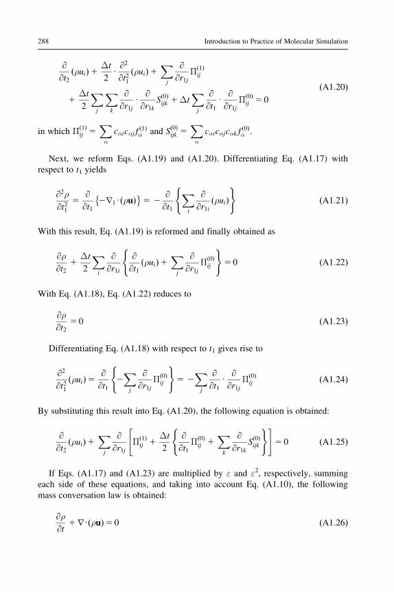
@
@t2ðρuiÞ1
Δt
2U@2
@t21ðρuiÞ1
Xj
@
@r1jΠð1Þ
ij
1Δt
2
Xj
Xk
@
@r1jU
@
@r1kSð0Þijk 1Δt
Xj
@
@t1U
@
@r1jΠð0Þ
ij 5 0
ðA1:20Þ
in which Πð1Þij 5
Xα
cαicαj fð1Þα and S
ð0Þijk 5
Xα
cαicαjcαk fð0Þα :
Next, we reform Eqs. (A1.19) and (A1.20). Differentiating Eq. (A1.17) with
respect to t1 yields
@2ρ@t21
5@
@t12r1UðρuÞ� �
5 2@
@t1
Xi
@
@r1iðρuiÞ
( )ðA1:21Þ
With this result, Eq. (A1.19) is reformed and finally obtained as
@ρ@t2
1Δt
2
Xi
@
@r1i
@
@t1ðρuiÞ1
Xj
@
@r1jΠð0Þ
ij
( )5 0 ðA1:22Þ
With Eq. (A1.18), Eq. (A1.22) reduces to
@ρ@t2
5 0 ðA1:23Þ
Differentiating Eq. (A1.18) with respect to t1 gives rise to
@2
@t21ðρuiÞ5 @
@t12Xj
@
@r1jΠð0Þ
ij
)5 2
Xj
@
@t1U
@
@r1jΠð0Þ
ij
(ðA1:24Þ
By substituting this result into Eq. (A1.20), the following equation is obtained:
@
@t2ðρuiÞ1
Xj
@
@r1jΠð1Þ
ij 1Δt
2
@
@t1Πð0Þ
ij 1Xk
@
@r1kSð0Þijk
( )" #5 0 ðA1:25Þ
If Eqs. (A1.17) and (A1.23) are multiplied by ε and ε2, respectively, summing
each side of these equations, and taking into account Eq. (A1.10), the following
mass conversation law is obtained:
@ρ@t
1rUðρuÞ5 0 ðA1:26Þ
288 Introduction to Practice of Molecular Simulation

From a similar manipulation of Eqs. (A1.18) and (A1.25), the momentum conversa-
tion law is obtained as
@
@tðρuiÞ1
Xj
@
@rjΠij 1
Xj
Δt
2U@
@rjε@
@t1Πð0Þ
ij 1Xk
@
@rkSð0Þijk
( )5 0 ðA1:27Þ
in which Πij � Πð0Þij 1 εΠð1Þ
ij :Finally, we derive another important equation. The variable transformation of
Eqs. (A1.10) and (A1.11) is conducted for Eq. (A1.6) to give
Δt ε@fα@t1
1 ε2@fα@t2
� �1
ðΔtÞ22
ε2@2fα@t21
1ΔtεðcαUr1Þfα
1ðΔtÞ22
ε2ðcαUr1ÞðcαUr1Þfα 1 ðΔtÞ2ε2ðcαUr1Þ@fα@t1
51
τð f ð0Þα 2 fαÞ
ðA1:28Þ
Substituting Eq. (A1.7) into this equation, collecting the terms of the order ε, andtaking these collected terms equal to zero then yields
21
τΔtf ð1Þα 5
@f ð0Þα
@t11
Xi
@
@r1iðcαif ð0Þα Þ ðA1:29Þ
Since f ð0Þα can be regarded as a function of the macroscopic quantities ρ and ρui,@f ð0Þα =@t can be reformed using Eqs. (A1.17) and (A1.18) as
@f ð0Þα
@t15
@f ð0Þα
@ρU@ρ@t1
1Xi
@f ð0Þα
@ðρuiÞU@ðρuiÞ@t1
5 2@f ð0Þα
@ρU
@
@r1UðρuÞ2
Xi
Xj
@f ð0Þα
@ðρuiÞU
@
@r1jΠð0Þ
ij
ðA1:30Þ
Substituting this equation into Eq. (A1.29) yields the required equation:
21
τΔtf ð1Þα 5 2
@f ð0Þα
@ρU
@
@r1UðρuÞ2
Xi
Xj
@f ð0Þα
@ðρuiÞU
@
@r1jΠð0Þ
ij 1Xi
@
@r1iðcαif ð0Þα Þ
ðA1:31Þ
Equations (A1.27) and (A1.31) are the basic equations for deriving the important
relationships in Chapter 8.
289Appendix 1

This page intentionally left blank

Appendix 2: Generation of RandomNumbers According to GaussianDistribution
In order to set the initial velocities of particles in MD simulations, or to generate
random displacements in BD and DPD simulations, it is necessary to generate ran-
dom numbers according to a particular probability distribution. The probability dis-
tributions of interest here are the Gaussian distribution (also known as the normal
distribution), and the Maxwell�Boltzmann distribution (or Maxwellian distribu-
tion). For example, since the velocity of particles theoretically has the Maxwellian
velocity distribution for thermodynamic equilibrium, as explained in Section 2.2,
the initial velocity of particles in simulations must have such a velocity distribu-
tion. We show the method of setting the initial velocity of particles according to
the Maxwellian distribution in the following paragraphs.
We assume that the stochastic variable x, such as the particle velocity or a ran-
dom displacement, obeys the following normal distribution ρ(x):
ρðxÞ5 1
ð2πÞ1=2σexp 2
ðx2 xÞ22σ2
� �ðA2:1Þ
in which σ2 is the variance and x is the average of the stochastic variable x.
In order to generate the stochastic variable x according to this normal distribution,
the following equations are used together with a uniform random number sequence
ranging from zero to unity:
x5 x1 ð22σ2 ln R1Þ1=2 cosð2πR2Þ or x5 x1 ð22σ2 ln R1Þ1=2 sinð2πR2ÞðA2:2Þ
According to either equation of Eq. (A2.2), the required number of values of the
stochastic variable are generated using a series of random numbers, such as R1 and
R2, taken from a uniform random number sequence. In this way, the initial veloci-
ties of particles and random displacements can be assigned. The technique in
Eq. (A2.2) is called the Box�Muller method [26].
For generating a uniform random number sequence, there is an arithmetic
method and a machine-generated method; the former is shown in the last subrou-
tine of the sample simulation program in Section 3.1.6. The arithmetic method is

reproducible, and the same random number sequence can be obtained at any time
in the simulations. In contrast, the machine-generated method is generally not a
reproducible sequence, and a different sequence of random numbers is generated
each time a simulation is run.
For the case of the Maxwellian velocity distribution, the velocity components of
particle i can be assigned using the random numbers R1, R2, . . ., R6 taken from a
uniform random number sequence as
vix 5 f22ðkT=mÞln R1g1=2 cosð2πR2Þviy 5 f22ðkT=mÞln R3g1=2 cosð2πR4Þviz 5 f22ðkT=mÞln R5g1=2 cosð2πR6Þ
9>=>; ðA2:3Þ
In this way, all the initial velocity components can be assigned using random
numbers.
292 Introduction to Practice of Molecular Simulation

Appendix 3: Outline of Basic Grammarsof FORTRAN and C Languages
We here do not aim to explain the entire grammar of the programming languages;
indeed, there is not sufficient space to do so. In each section of programming lan-
guage, the main structure of a program is first explained in order to understand the
logical framework of a program. Then, such important grammar as control state-
ments is explained. Finally, several points of interest that may be outside of the
main body of a program will be addressed. This will be followed by a short sample
program that demonstrates the essence of a research simulation program and
explains the grammar used in the program in detail. This approach is most effec-
tive, because the grammar is explained in relation to the logical flow of a simula-
tion program. The skill to develop a simulation program has a strong relationship
with the ability for embodying a logical flow using a programming language.
A3.1 FORTRAN Language
The general structure of a program written in the FORTRAN language is composed
of a main program together with subroutine subprograms or function subprograms,
as shown below.
123456789… …72
IMPLICIT REAL*8 (A-H, O-Z), INTEGER (I-N)PARAMETER( NN=8) REAL*8 RX(NN), RY(NN)REAK*8 VX(NN), VY(NN) INTEGER N
STOPEND
Main program
Description of calculation procedures

SUBROUTINE INIPOSIT(N,H)
RETURNEND
SUBROUTINE INIVEL(N)
RETURNEND
REAL*8 FUNCTION PRESSURE(H)
RETURNEND
Subroutine subprogram
Function subprogram
Subroutine subprogram
Description of calculation procedures
Description of calculation procedures
Description of calculation procedures
A main program first needs to be constructed, and then subroutine or/and func-
tion subprograms necessarily follow the main program. The main program begins
with the definition of the variables and finishes with the STOP and END statements
that are placed at the end to halt the execution of the program. A subroutine or
function subprogram begins with a SUBROUTINE (name of a subroutine) or (pre-
cision) FUNCTION (name of a function) statement, respectively, and finishes with
the RETURN and END statements that signal the return to the task of the main
program. A main program must be written in such a way that the logical flow is
clear, and calculations that disturb this logical flow should be treated in subroutine
or function subprograms. In other words, when a program is constructed in such a
way that a reader is able to grasp the logical flow in a straightforward manner, it
becomes more than a hobby program—it becomes a common useful tool. This is
an important consideration for developing a simulation program with contributions
from and used by different persons in a successive research project.
In a subroutine subprogram, routine calculations are carried out. The calculation
task moves from a main program to a subroutine subprogram by calling the name of
the subroutine (the CALL statement) and returns to the main program on meeting
the RETURN statement in the subroutine. A function subprogram is quite similar to
a subroutine subprogram in that routine calculations are carried out in an area (the
subprogram) aside from the main program. The difference between the two is that in
a function subprogram the name of the function subprogram itself assumes a calcu-
lated value, and this value is passed to the main program by simply referring to the
name of the function subprogram in the main program. In other words, the name of
a function subprogram is treated as a variable in a main program: the calculation
294 Introduction to Practice of Molecular Simulation

task moves to a function subprogram at the time of meeting its name, and returns to
the main program with a value calculated there on meeting the RETURN statement.
Hence, a CALL statement is unnecessary in order to move to a subprogram area.
These are the main points of the program structure and flow of the calculation proce-
dures. There is an important point concerning the data transfer between a main pro-
gram and a subprogram. In the FORTRAN language, information regarding the
value of variables cannot be transferred between a main program and a subprogram
unless definite descriptions are written for that purpose. There is a significant differ-
ence between the FORTRAN and the C language in this respect. We explain the
method of transferring data between a main program and a subprogram in detail
later.
As shown in the preceding example, main sentences generally have to be written
between the 7th and 72nd columns in a FORTRAN77 program. The first column is
used for defining whether or not that line is a comment line (that does not influence
calculations) by employing a C character or a blank; the sixth column is for defin-
ing whether or not the line is regarded as a continuation line from the previous line
by the “&” character or blank; and the area between the 2nd and 5th columns is
used for writing figures (or labels) of the end statements, such as the CONTINUE
statement or of an indication of the destination of the GOTO statement. Various
examples of this type of use can be seen in the sample simulation programs, and
therefore we omit such explanations here.
• This is the simplest IF statement, andTHEN is unnecessary in this case.
IF(X.GT.0.D0)A=B+10.D0
IF(X.GT.0.D0)THEN …END IF
IF(X.GT.0.D0)THEN …ELSE …END IF
IF(X.GT.0.D0)THEN …ELSE IF(X.LE.-10.D0) THEN …ELSE…END IF
IF(X.GT.0.D0)THEN …ELSE IF(X.LE.-10.D0) THEN …ELSE IF(X.EQ.-5.D0) THEN…END IF
• Execution only for X>0.
• One of separate procedures is chosenfor X>0 or X≤0.
• One of three separate procedures ischosen for X>0 or X≤–10 or the othercases.
• One of three separate procedures ischosen for X>0 or X≤-10 or X=–5.
295Appendix 3

We now explain the IF and DO statements, which are perhaps the most impor-
tant control statements for developing a calculation program. The IF statement is a
control statement to select a calculation procedure by assessing the condition. The
DO statement is a control statement to repeat a certain procedure a prescribed num-
ber of times. Typical examples of the IF statement are shown above. The IF state-
ment implies the execution of a certain procedure if a condition is satisfied;
another procedure is carried out if it is not satisfied. In the above examples, the first
IF statement is the simplest and the following examples become more complex.
Several IF statements can be combined to make a complex assessment, and such
examples may be found in the sample simulation programs. In the IF statement, LT
and LE imply , and # , respectively; GT and GE imply . and $ , respectively;
and EQ and NE imply 5 and 6¼, respectively. The statement for repeating proce-
dures is the DO statement. Several representative examples of the DO statement
are shown in the following.
DO 30 I=N,1,-2 … 30 CONTINUE
DO 90 I=-N,N+1,5 … 90 CONTINUE
DO 20 I=1,N … 20 CONTINUE
• The procedure starts at I=1, then is conducted at I=2 and continued until I=N.• The procedure starts at I=N, then is conducted at I=N-2 and continued at I=N-4, N-6, ….
• The procedure starts at I=-N, then is conducted at I=-N+5, I=-N+10, …, until I becomes over N+1.
The DO statement implies that the procedure written between DO and
CONTINUE is executed until the index arrives at the required end value. In the
above example, I is the index and N is the end value of the loop. In the first exam-
ple, the index I changes in the sequence I5 1, 2,. . ., N. In the second example, the
index I changes in the sequence I5N, N2 2, N2 4,. . .; if N is even, the proce-
dures are repeated until N5 2, and if N is odd, they are repeated until N5 1. The
last example shows that a negative value, 2N, is possible as a starting value of the
index I. Either specific numbers or variables are possible for the starting and ending
values and the increment interval value of the DO loop statement. Be aware that
although REAL variables can be used as an index of the DO loop, INTEGER vari-
ables are desirable in order to remove any ambiguity in relation to the assessment
concerning the termination of the DO loop. In order to move out of the DO loop at
any time before the designed end, the GOTO statement employed with the previous
IF statement may be used. A final point to be noted relating to the DO loop is that
in the first above example, the index I does not have the figure N but (N1 1) for
the end of the procedure; thus, care should be taken in using the variable I in the
next task. Using variables in this way should be avoided in order to prevent causing
an unexpected error.
296 Introduction to Practice of Molecular Simulation

Next, we explain several types of grammar that are relatively difficult to
understand when learning the FORTRAN language. First, we explain how to
transfer the values of variables between the main program and a subprogram. In
FORTRAN, there are two methods for the data transfer: (1) the values of vari-
ables are transferred to a subprogram through the arguments of the subprogram,
and (2) the variables to be transferred between a main program and a subpro-
gram are declared with the COMMON statements so that they can be accessed
from both the main program and the subprograms. An example of the former
method is as follows:
CALL INIVEL(N,H,T). . .SUBROUTINE INIVEL(N,H,T). . .
In this case, the values of the variables N and H are transferred from a main
program to a subprogram, and the procedure returns to the main program with a
value of T, which was calculated in the subprogram. A big difference between
FORTRAN and the C language is that in the former language new values of N
and H, which were changed in the subprogram, are reflected in the main pro-
gram, but in the latter language this never arises unless a specific direction is
given to do so. This will be explained in detail later in the grammar of the C
language.
The second method for the data transfer is to use the COMMON statement: the
variables declared in the COMMON statements can be accessed from both the
main program and all the subprograms without any need for specific statements for
the data transfer. An example is as follows:
PARAMETER (NN5100)COMMON /BLOCK1/ N, RX, RYREAL*8 RX(NN), RY(NN), HINTEGER N. . .CALL INIVEL(H). . .STOPEND. . .SUBROUTINE INIVEL(H)PARAMETER (NN5100)COMMON /BLOCK1/ N, RX, RYREAL*8 RX(NN), RY(NN), HINTEGER N
297Appendix 3

. . .RETURNEND
In a main program, the variables, which are used in subprograms, can be defined
in the COMMON statements before the definition of other standard variables.
By defining the same variables in the COMMON statements in a subprogram,
the values saved on the variables can be referred to; also, new values may be
saved on these variables. In the above example, the values of N, RX(*), and
RY(*) are transferred using the COMMON statement, and a value of H is trans-
ferred as an argument. Note that the names of the variables in the COMMON
statements are not necessarily the same, but we recommend that the beginner
use the same names until they obtain a more complete understanding of the
language.
Another feature that the beginner may find difficult is the WRITE and
FORMAT statements. These statements are used for outputting results to a data file
and have no relation to the execution of the calculations. The following example is
for outputting the data for the purpose of confirming either the final or intervening
results of the calculation:
I53XI55.D0YI52.D0PRESS5XI*YIWRITE(NP,20) I, XI, YI,PRESS
20 FORMAT(’I5’,I3,3X,’XI5’,F7.3,2X,’YI5’,F7.3,2X,& ’PRESSURE AT (XI,YI)5’, F10.3)
The result of the output from this FORMAT statement is as follows:
I5 3 XI5 5.000 YI5 2.000 PRESSURE AT (XI,YI)5 10.000
The above example is a part of the program for outputting the data of the vari-
able PRESS, which is obtained by multiplying XI by YI. For the case of
NP5 6, the results are output to the display of the computer, and if the OPEN
statement relates the device number (or device unit number) NP with a data
file, the result is output to the data file. For example, if “OPEN (11,
FILE5 ‘faa1.data’, STATUS5 ‘UNKNOWN’)” is declared and NP is set as
NP5 11, the data is output to the file faa1.data. Since the results shown on a
display can be seen only once, data is usually output to a data file. Inside the
298 Introduction to Practice of Molecular Simulation

parentheses of the FORMAT statement, I3 means that the output is an integer
and is output up to three spaces (columns) to the right of the space, F7.3 means
that the output is a real number and is output using 7 spaces (columns), in
which the number is rounded to three decimal places and is written to the right
of the space; 3X means that three blank spaces are to be inserted. The reader
can see many examples of FORMAT statements in the sample simulation pro-
grams in Chapters 3�7.
A long run of the execution of a simulation program is sometimes divided into
several short runs. For this case, the intervening results are output to a data file,
and the following run is carried out to continue from the previous run using the
data saved in the file. This data may also be used for visualizing a particle configu-
ration in a form such as a snapshot. To do so, only numerical data is suitable for
the output to a data file—that is, without the specification of the names of the vari-
ables. A typical example is as follows:
. . .WRITE(NP,50) N
50 FORMAT( I8 )WRITE(NP,55) (RX(I),I51,N), (RY(I),I51,N)
55 FORMAT( (5E16.8) )
In the above example, the data saved in the array-type variables RX(*) and RY(*)
are output using a simple specification without using the DO statement. The speci-
fication of (5E16.8) in the FORMAT statement means that five data are output in
one line. The outer bracket ( ) is used for the repetition of the output specification
5E16.8, which means that the output data is real and is output using 16 spaces (col-
umns) in which the data is written to the right of the space with 8 decimal places.
In order to continue a separate successive run using the data which is output in the
above example, we need to use the following READ statement for reading the nec-
essary data:
READ(NP1,60) N60 FORMAT( I8 )
READ(NP1,65) (RX(I),I51,N), (RY(I),I51,N)65 FORMAT( (5E16.8) )
An important point is that the same FORMAT statement must be used for the
WRITE and READ statements; otherwise, the exact numerical values cannot be
read by the READ statement.
Finally, to assist the reader in understanding the grammar in more detail, we
have added explanatory remarks to the following sample program, which was made
by compressing a full simulation program.
299Appendix 3

0001 C**************************************************************** 0002 C* diffuse_sample.f (not complete version) * 0003 C* * 0004 C* MOLECULAR DYNAMICS METHOD FOR MOLECULAR DIFFUSION PROBLEM * 0005 C* --- TWO-DIMENSIONAL CASE --- * 0006 C* * 0016 C**************************************************************** 0033 IMPLICIT REAL*8 (A-H,O-Z), INTEGER (I-N) 0034 C 0035 COMMON /BLOCK1/ RX0 , RY0 , RX , RY 0036 COMMON /BLOCK2/ FX , FY 0040 C 0041 PARAMETER( NN=80, NRANMX=50000 ) 0042 PARAMETER( PI=3.141592653589793D0 ) 0043 C 0044 REAL*8 RX0(NN), RY0(NN), RX(NN) , RY(NN) 0045 REAL*8 FX(NN) , FY(NN) , VELX(NN), VELY(NN) 0046 REAL*8 H , RC , L , T , K , NDENS 0047 C 0048 REAL RAN(NRANMX) 0049 INTEGER NRAN , IX 0050 C 0051 REAL*8 RXI, RYI, TIME, HSQ, CC0, CC1 0052 INTEGER N, NA, NB 0055 C 0056 OPEN( 9,FILE= '@aaa1.data',STATUS='UNKNOWN') 0057 OPEN(21,FILE='aaa001.data',STATUS='UNKNOWN') 0058 OPEN(22,FILE='aaa011.data',STATUS='UNKNOWN') 0062 NP=9 0063 C ----- PARAMETER (1) ----- 0064 T = 5.0D0 0065 K = 10.D0 0066 NA = 20 0072 L = DSQRT( DBLE(N)/NDENS ) 0073 HSQ = H*H 0079 C ----- PARAMETER (3) ----- 0080 IX = 0 0081 CALL RANCAL( NRANMX, IX, RAN ) 0082 NRAN = 1 0083 C 0084 C --------------------------------------------------------- 0085 C --------------- INITIAL CONFIGURATION --------------- 0086 C --------------------------------------------------------- 0087 C 0100 C --- CAL PREVIOUS POSITION --- 0101 CALL POSITR1( N, NA, H, K ) 0102 C 0103 C --- PRINT OUT CONSTANTS --- 0104 WRITE(NP,5) T , K , NDENS , NA , NB , L , H , RC 0105 C --- PRINT OUT INITIAL CONFIGURATION --- 0109 C --------------------------------------------------------- 0110 C --------------- START OF MAIN LOOP
• IMPLICIT is the implicit data type declaration. In this case, the variables with their name starting with one of A~H and O~Z are regarded to be a double-precision real, and similarly those with one of I~N are regarded to be an integer.
• The variable defined in the COMMON
statement can be accessed from everywhere without transferring them into subprograms as arguments. In the case of array variables, the dimension must be defined in the data type statement.
• The PARAMETER statement is frequently used for defining the variables used for specifying the dimensions of array variables; the change of these values in PARAMETER enables us to change the dimensions of the related array variables.
• REAL*8, REAL, and INTEGER are the data type declaration statements for double-precision reals, single-precision reals, and integers, respectively. Although a computer can usually treat integers only between ± several ten billions, the INTEGER*8 statement enables one to use a much wider range of integers. Double-precision reals may be sufficient in scientific computations, but quad-precision reals are appropriate in some cases.
• OPEN statements can relate data files to the input/output devices; CLOSE statements must be used together. The number 5 is the keyboard, 6 is the display, and other numbers are used for data files (numbers larger than 8 may be desirable). OLD in the STATUS statement implies an already-existed file.
• Double-precision reals are expressed for example 5.2D0 or 0.052D2; single-precision reals are expressed such as 5.2 or 0.052E2. DSQRT means the square root, and * means the multiplication.
• The line number is added for convenience and the first column starts from the position of C character. The C in the first column implies that the line is just a comment.
• The subroutine POSITR1 is called by the CALL statement.
The variables necessary in the subroutine are passed as
arguments (N, NA, H, K); the description of these variables
has to be described in this order in the subroutine subprogram.
• The data are written out in the format expressed in the 5
FORMAT statement; these statements should be placed before
the STOP statement.
300 Introduction to Practice of Molecular Simulation

0111 C --------------------------------------------------------- 0114 C 0115 DO 100 NTIME=1, NTIMEMX 0116 C 0121 DO 50 I=1,N 0122 C 0123 IF ( I .EQ. NA+1 ) CC1 = CC0 0124 RXI = 2.D0*RX(I) - RX0(I) + FX(I)*HSQ*CC1 0126 RX0(I) = RX(I) 0128 RX(I) = RXI 0130 C 0131 50 CONTINUE 0132 C --- PRINT OUT DATA --- 0133 IF ( MOD(NTIME,NPRINT) .EQ. 0 ) THEN 0134 TIME = H*DBLE(NTIME) 0135 CALL PRINTOUT( N, NA, TIME, NP ) 0136 END IF 0141 C 0142 DO 60 I =1,N 0143 IF( I .LE. NA ) THEN 0144 R = 1.D0 0145 ELSE 0146 R = 1.5D0 0147 END IF 0148 WRITE(NOPT,58) I, R, RX(I), RY(I) 0149 60 CONTINUE 0153 C 0154 100 CONTINUE 0155 C 0156 C ------------------------------------------------------- 0157 C ------------------ END OF MAIN LOOP ---------------- 0158 C ------------------------------------------------------- 0159 CLOSE(NP, STATUS='KEEP') 0160 C 0161 C ---------------------- FORMAT -------------------------- 0162 5 FORMAT(/1H ,'------------------------------------------' 0163 & /1H ,' MOLECULAR DYNAMICS SIMULATION ' 0164 & /1H ,'FOR TWO-DIMENSIONAL MOLECULAR DIFFUSION PROBLEM' 0165 & /1H ,'-------------------------------------------' 0166 & /1H ,'TEMPERATURE=',F6.2 ,2X, 'MASS RATIO=',F6.2 ,2X, 0167 & 'NDENS=',F6.3 0168 & /1H ,'NUMBER OF MOLECULES OF SPECIES A=',I4 0169 & /1H ,'NUMBER OF MOLECULES OF SPECIES B=',I4 0170 & /1H ,'MAGNITUDE OF CAGE=',F7.2 ,2X, 'TIME DIFF.=', 0171 & F8.5 ,2X, 'CUTOFF RADIUS=',F6.2/) 0172 56 FORMAT( 3I6, 2E13.8 ) 0173 58 FORMAT( I5, F8.3 , 2E26.18 ) 0174 C 0175 STOP 0176 END 0177 C************************************************************ 0178 C********************* SUBROUTINE ********************* 0179 C************************************************************ 0180 C 0380 C**** SUB POSITR1 **** 0381 SUBROUTINE POSITR1( N, NA, H, K ) 0382 C 0383 IMPLICIT REAL*8 (A-H,O-Z), INTEGER (I-N) 0384 C 0385 COMMON /BLOCK1/ RX0 , RY0, RX, RY 0386 COMMON /BLOCK2/ FX , FY 0387 COMMON /BLOCK3/ VELX, VELY 0388 C 0389 PARAMETER( NN=80 ) 0390 C 0391 REAL*8 RX0(NN), RY0(NN), RX(NN) , RY(NN) 0392 REAL*8 FX(NN) , FY(NN) , VELX(NN), VELY(NN) 0393 REAL*8 H , K 0394 REAL*8 HSQ2, CC0, CC1
• The DO loop implies the iteration calculation; the statements between DO and CONTINUE are repeatedly carried out. The procedure starts at NTIME=1, and then is conducted at NTIME=2, 3,···, until I=NTIMEMX. DO loops are possible inside the DO loop.
• MOD(NTIME, NPRINT)returns the remainder after NTIME is divided by NPRINT. DMOD is used for such an operator of double-precision reals. As in this example, operators have a slightly different name depending on the data type of variables.
• DBLE(*) is used for transforming an integer into a double- precision real. For developing a universal program, it is desirable that the data types be the same between the left and right-hand sides in the equation. INT(*) is used for transform-ing a double-precision real into an integer.
•One of the procedures is chosen after assessing the IF statement. In this example, R=1.D0 if I≤NA, and R=1.5D0 if I>NA.
• The data file opened by the OPEN statement must be closed using the CLOSE statement. NP is the device number (name) of the I/O device, which is used to open the data file. KEEP is used in the STATUS statement in almost all cases.
• The variables are described in the same order in which they have been written in CALL POSITR1.
• IMPLICIT, PARAMETER, and REAL*8
statements are described in the same way as in
the main program. The subroutine can access
the variables in the COMMON statements, as well
as the arguments of N, NA, H, and K; note
that the change in these variables in the
subroutine is reflected in the main program.
The other variables are valid only in this
subroutine, and never affect the main program.
• The collection of FORMAT statements before the STOP statement makes the logical structure of calculations clearer. • / on the first line means the insertion of one blank line; / in the later lines mean starting a new line. “1H ,” means one blank space indent in each line. “56 FORMAT” and “58 FORMAT” are for writing out only numerical data (or figures).
301Appendix 3
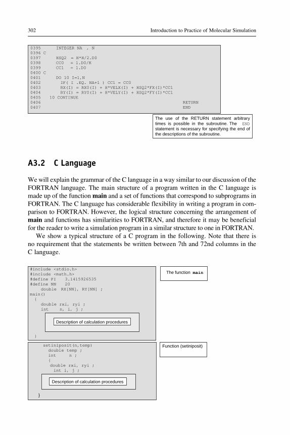
0395 INTEGER NA , N 0396 C 0397 HSQ2 = H*H/2.D0 0398 CC0 = 1.D0/K 0399 CC1 = 1.D0 0400 C 0401 DO 10 I=1,N 0402 IF( I .EQ. NA+1 ) CC1 = CC0 0403 RX(I) = RX0(I) + H*VELX(I) + HSQ2*FX(I)*CC1 0404 RY(I) = RY0(I) + H*VELY(I) + HSQ2*FY(I)*CC1 0405 10 CONTINUE 0406 RETURN 0407 END
The use of the RETURN statement arbitrary times is possible in the subroutine. The END statement is necessary for specifying the end of the descriptions of the subroutine.
A3.2 C Language
Wewill explain the grammar of the C language in a way similar to our discussion of the
FORTRAN language. The main structure of a program written in the C language is
made up of the functionmain and a set of functions that correspond to subprograms in
FORTRAN. The C language has considerable flexibility in writing a program in com-
parison to FORTRAN. However, the logical structure concerning the arrangement of
main and functions has similarities to FORTRAN, and therefore it may be beneficial
for the reader to write a simulation program in a similar structure to one in FORTRAN.
We show a typical structure of a C program in the following. Note that there is
no requirement that the statements be written between 7th and 72nd columns in the
C language.
setiniposit(n,temp) double temp ; int n ; {
double rxi, ryi ; int i, j ;
}
Description of calculation procedures
Function (setiniposit)
#include <stdio.h> #include <math.h> #define PI 3.1415926535 #define NN 20 double RX[NN], RY[NN] ; main() {
}
double rxi, ryi ; int n, i, j ;
The function main
Description of calculation procedures
302 Introduction to Practice of Molecular Simulation

setinivel(n,press) double press ; int n ; {
double vxi, vyi ; int i, j ;
}
Function (setinivel)
Description of calculation procedures
The function main is placed first, and other functions, corresponding to
subprograms in FORTRAN, follow main. The main body of the statements in
each function begins with the notation { and ends with the notation }. Since
there is no limit on the number of characters in one line, the notation ; is
used for terminating a line of statement—that is, it means the end of the line.
Except for special statements, every line must end with such a notation ;.
Because mathematical functions such as sin and sqrt are necessarily used in
scientific calculations, the statement of #include ,math.h. needs to be
declared in the first description area. Also, the statement of #include , stdio.h.is indispensable to any program to facilitate the input or output of data to a
display or data file, and for reading data from a keyboard or data file. The
statements of #define PI 3.14. . . and #define NN 20 correspond to the
PARAMETER statement in FORTRAN. A statement beginning with the nota-
tion # is a preprocessor directive, which is a command to the compiler’s pre-
processor that treats instructions before the compilation procedure starts. The
preprocessor directive of #define NN 20 implies that the value of 20 is
assigned to the variable NN. The next statement, corresponding to the
COMMON statement in FORTRAN, is the declaration of the array-type vari-
ables RX[NN] and RY[NN] being used as global variables (which can be used
in the other function programs with no further definitions). The C language
typically uses lower-case characters, but it may be best that the names of
global variables are declared using upper case, so a programmer can be more
aware of treating the global variables. In a way similar to FORTRAN, the exe-
cution of a program starts with the function main; the procedures move to a
function when the function name is met and return to the main program
(main) after completion of the procedures in the function. As seen in this
explanation, the C language does not need the CALL statement used in the
FORTRAN language for transferring the task to another function. It employs
only the name of the function. The function main is written in a way to clar-
ify the flow of calculations, whilst any complex calculation procedure is
recommended as a separate function.
Next, we explain the most important statements for developing a program: the
if, for, do while, and switch statements. We first explain the if statement, which is
303Appendix 3

used for choosing tasks according to certain conditions specified by the instruc-
tions. Some typical examples are as follows:
if(i= =3) x=a ;
if( x>=0.) z=b ; else if( x<-10. ) z=c ; else z=d ;
if( x>=5. ) { z=a1 ; }
if( x>5. ) { z=a1 ; }else if( x<=-10. ) { z=b1 ; }else { z=c1 ; }
if( (x>=-10.) && (X<=10.) ) { z=a1 ; } else if( (x>=50.)||(x<=-50.) ){ z=b1 ; }
• This is the simplest if statement. “i=3” is expressed as “i==3” in the Clanguage.
• If x≥0, z=b is set, if x<-10, z=c, and z=d for the other cases.
• This is a block-type if statement.
• This is also a block-type if statement. One procedure is chosen depending on the condition; there are three cases x>5, x≤-10, and the other cases.
• This is also a block-type if statement. “&&” means that if both the conditions are satisfied, z=a1 is assigned and “| |” means that if one ofthe conditions at least is satisfied, z=b1 is assigned.
The if statement implies that the procedure is carried out if a certain condition
specified in the if statement is satisfied; otherwise, another assessment or another
procedure (including the end of the execution of the if directive) is conducted. The
specification “, 5 ” in the condition statements represents the mathematical
meaning # , “. 5 ” means $ , “5 5 ” means 5 , and “!5 ” means 6¼. We next
explain the statements of for, while, and do while, which are used for specifying
the repeating procedures. Several typical examples follow.
for(i=1; i<=n; i++) { … ;
}
for(i=100; i>=0; i-=2) { … ;
}
i=3 ; do { xnew = xold + xdef ; i++ ; } while( i<=n ) ;
i=3 ; while( i<=n ) { xnew = xold + xdef ; i++ ; }
• The procedure starts at i=1, then is conducted at i=2 and continued until i=n.
• The procedure starts at i=100, and is conducted at i=98, 96,…, while i≥0. “i–=2” means“i=i–2.”
• The procedure starts at i=3 and is conducted at i=4,5, …, while i≤n. “i++” means “i=i+1” and “i––” means “ i=i–1.”
• The procedure is the same as in the previous case, but terminating the procedure is assessed in a different position.
304 Introduction to Practice of Molecular Simulation

The above statements correspond to the DO statement in FORTRAN. The proce-
dures specified between { and } are repeated, with the value of the index variable i
increasing or decreasing after the execution of each cycle step. The way of chang-
ing the index value is specified by the statement between ( and ) in the for state-
ment, such as “i11 ” or “i25 2”. In the case of the do while and while
statements, the way of changing the index value is specified by “i11 .” If the
statement of “i15 3” is used, the index i will change so that “i5i13.” A differ-
ence between the do while and the while statements is the position for assessing
the termination of the procedures. The procedure specified between { and } is
repeatedly carried out, whilst the condition indicated in the while statement
is satisfied.
A statement with characteristics similar to if is the switch statement. This state-
ment is quite simple to use; an example follows:
switch (itree ) { case 2 ; x = a1 ; y = b1 ; break ; case 3 ; x = a2 ; y = b2 ; break ; default ; x = a4 ; y = b4 ; break ;}
• When itree=2, a series of
statements defined in “case 2” are
executed, and break means the exit
from the switch statement. A similar
procedure is carried out for “case 3.”
In the other cases, a series of
statements defined in default are
executed; the break statement is
possibly unnecessary in the default
area.
As already pointed out, the function main and other functions correspond to a
main program and subprograms in the FORTRAN language, respectively. There
are two types of functions in the C language. That is, the first type of function cor-
responds to a function subprogram in the FORTRAN language, and therefore a
value calculated in the function is transferred through the variable (i.e., the name of
the function) in the function main. The second type of function corresponds to a
subroutine subprogram, and a value calculated there is not transferred through the
name of the function. Several examples that explain these two types of functions
are shown here:
setinivel(n,press) double press ; int n ; { double vxi, vyi ; int i, j ; … }
• This is a function that returns no calculated values to the main function. It corresponds to the subroutine subprogram in FORTRAN.
305Appendix 3

double press(x, y) double x, y; { double c1, c2, cans ; c1=1. ; c2=2. ; cans = c1*x + c2*y ; return( cans ) ; }
int press(x,y) double x, y ; { int ic, jc, ians ; ians = ic*(int)x + jc*(int)y ; return( ians ) ; }
• This corresponds to the function subprogram in FORTRAN; the calculated value “cans” is substituted into the double-precision variable “press,” and the value of “press” is returnedto main.
• This also corresponds to the integer function subprogram in FORTRAN; the calculated value “ians” is substituted into the integer variable “press,” and the value of “press” is returned to main.
In the second and third examples, a value calculated in the function is transferred
to the main program main through the function name. The descriptor of the func-
tion type, such as double and integer, is, therefore, attached before the function
name. In the first example, the function does not return a calculated value to the
main program, but certain procedures are carried out in this function, so that
the declaration of the function type is unnecessary and not attached to the function
name. Note that int, float, and double imply that a variable (or data) is integer-
type, single-precision-real-type, and double-precision-real-type, respectively.
Next, we explain several important points that seem to be relatively difficult or
may be misunderstood by the beginner who is learning the grammar of the C lan-
guage. Array-type variables are defined in the declaration statements of the data
type in such a way as double a[100] or rx[20][20]. For example, in the case of a
one-dimensional array such as double a[100], it is noted that a[0], a[1], . . ., a[99]storage spaces are prepared, but a[100] is not available. The second example of
double rx[20][20] means the declaration of a two-dimensional array variable, and
rx[0]][0], rx[0][1], rx[0][2], . . ., rx[19][19] storage spaces are prepared.A significant difference between FORTRAN and the C language concerns the data
transfer between the function main (main program) and other functions (subpro-
grams). In FORTRAN, when one transfers data to a subprogram as arguments, one
does not take the values themselves saved in the variables but rather takes the positions
or addresses of the variables in which the data are saved. This means that the values
saved in the variables can freely be accessed from the subprogram, and also that new
data can be assigned to such variables; these new values are reflected in the main pro-
gram. This data transfer type is the “call by reference.” In the case of the C language,
the specification of variables as arguments, as in the FORTRAN language, does not
mean the transfer of the address of the variables; rather, the values themselves saved in
the variables are transferred to the function; therefore the assignment of new values to
the variables in the function is never reflected in the main program. This type of data
transfer is the “call by value.” This means that in respect to data transfer, the C lan-
guage is much safer than FORTRAN. If the data transfer is carried out by “call by ref-
erence” in a similar way to FORTRAN, then the variables of the “pointer” class must
be used in the C language. A pointer variable saves the position or address of a stan-
dard variable, and therefore it is important to declare what type of data is saved at the
306 Introduction to Practice of Molecular Simulation

position. For example, if an integer value is to be saved in a variable, the address of
which a pointer variable “pa” saves, then the asterisk * must be attached to the pointer
variable like “*pa,” and the data type must be declared like “int *pa.” In the body of
the program, the variable “*pa” is treated as a standard integer variable. If “int *pb,
ix” is declared in the definition statement of the data types, the statement “pb5&ix” is
used in order to save the address of the integer variable “ix” in the pointer variable
“pb.” If “&” is attached to a standard variable, for example, “&ix,” it will return the
value of the address of the variable ix. Therefore, since a pointer variable—for exam-
ple, “pa”—has the information about the address of a standard variable, a value (data)
saved at the address of the standard variable can be extracted using the notation “*pa.”
We are now ready to begin the explanation of “call by reference.”
In order to return from a function with the calculated values, the information of
the addresses of the variables, in which the calculated values are saved, need to be
transferred to the function by using arguments of the pointer type. For example,
consider a sample program in which a calculation is carried out using a value saved
in the variable “h” in the function “anscal,” and the calculated data is returned to
the main program through the variable “ans.” One has to call the function using the
statement “anscal (h, &ans),” in which a value (i.e., not the pointer information)
saved in the variable “h” is transferred to the function “anscal,” and the address of
the variable “ans” can be transferred to the function using the pointer information
“&ans.” It is important that the data type of the variable “*ans” is declared in the
function “anscal,” so that the variable “*ans” can be treated as a standard variable
in the function. Several typical examples (including a bad example) follow.
• The address of “ans” is transferred to the function; “&ans” is the address of the variable “ans.” In the function, the pointer variable “pans” is used for receiving the value of “ans” in the main function. Since “ans” is a double-precision real, “*pans” has to be defined as a double-precision-real variable.
double h, ans ;
x = anscal(h, &ans) ;
anscal(h, pans) double h, *pans ; { *pans = h*h ; }
double h, ans ;
x = anscal(h, ans) ;
anscal(h, ans) double h, ans ; { ans = h*h ; }
double h, ans[100] ;
x = anscal(h, ans) ;
anscal(h, ans) double h, ans[100] ; { for( i=0, i<=99; i++) { ans[i] = h*(dble)i ; } }
• This is a bad example. In this case the values saved in “h” and “ans” are transferred to the function “anscal,”but the values calculated in the function can never be returned (reflected) to the main function.
• For array variables, the data transfer to the function is quite similar to FORTRAN; the pointer variables are unnecessary for the data transfer for the case of array variables. The variable name itself is used as an argument in calling the function and also in the definition of the function name.
307Appendix 3

In the first example, the address of the variable “ans” in the main program is trans-
ferred as an argument “&ans.” This value is saved in the pointer variable “pans” in
the function; the data type of the variable “ans” is recognized in the function by
declaring “double *pans” there. Through these statements, the original value saved
in the variable “ans” in the main program is changed into a new value after this
new value is substituted into the variable “*pans” in the function. Clearly identify-
ing pointer variables from standard variables by attaching the asterisk * may signif-
icantly assist the programmer by removing the danger of mistakes arising from
substituting new values to those variables in other functions.
The second example demonstrates a bad example of programming, where new
values calculated in the function “anscal” are not transferred to the variables “h”
and “ans” in the main program, since the connection of the variables between the
main function and the function “anscal” can never be made using a statement of
the type “anscal (h, ans).” If the arguments are defined without pointer variables,
then a function that returns a calculated value to the main program may be used, as
already explained; in this case, “anscal (h, ans)” has to be changed into “double
anscal (h, ans),” and “return (ans);” is added to the line after “ans5 h*h;,” which
corresponds to a function subprogram in the FORTRAN language.
The third example demonstrates how to transfer values saved in array-type vari-
ables such as “ans.” The data transfer of array-type variables can be conducted in the
same way as for the FORTRAN language, and therefore pointer variables are unneces-
sary. That is, calling a function with the arguments that are array-type variables will
have a direct type of connection, so that new values assigned to the array-type vari-
ables in the function are reflected inmain without the need for pointer variables.
We have shown the three methods of returning calculated values from a function
back to the main function. The first method is to use pointer variables; the second is
to use array-type variables; and the third is to use a function that returns a calculated
value through the name of the function itself. In addition to these three methods is
another method that uses global variables that correspond to variables declared in
the COMMON statements in FORTRAN. The global variables have to be declared
before the “main( )” statement, and for these variables we recommend the use of
capital characters in their names, to help the programmer recognize them. An exam-
ple of using global variables is in the sample simulation program shown in
Section 5.6 as the array-type variables such as RX[NN], RY[NN], and RZ[NN].
Next, we explain the statements for inputting data, scanf and fscanf statements,
and for outputting data, printf and fprintf statements. The scanf and printf state-
ments correspond to READ(5,*) and WRITE(6,*) statements in FORTRAN; in these
statements, data are input from a keyboard and results shown on a display. In the
case of the fscanf and fprintf statements, data files are used for reading and writing
the data. If the reader understands the latter reading and writing statements, the for-
mer statements are quite straightforward to understand, so we only focus on the
explanation of the fscanf and fprintf statements. In order to use data files, pointer
variables must be connected to the data files used in a program. To do so, the fopen
statement is used, and fclose must be used to disconnect the data file used before the
end of the main program; this means that a data file connected by the fopen state-
ment should always be disconnected in a program. Some examples follow.
308 Introduction to Practice of Molecular Simulation

main(){
double a, b, c;int i;FILE *fopen(),*np1,*np2,*np[4];
np15fopen(”aaa0.data”,”r”);np25fopen(”aaa1.data”,”w”);np[1]5fopen(”bbb1.data”,”w”);np[2]5fopen(”bbb2.data”,”w”);np[3]5fopen(”bbb3.data”,”w”);
. . .fscanf(np1,”%lf”, &c );fprintf(np2,”a5%10.3f b5%10.3f\n”, a, b);i52;fprintf(np[i],”a5%10.3f b5%10.3f c5%10.3f\n”,a,b,c);
. . .fclose(np[1]);fclose(np[2]);fclose(np[3]);fclose(np1);fclose(np2);
As shown in the above example, a data file must be connected to the file pointer vari-
able, which is declared in the FILE statement, by using the fopen statement. After a
data file is opened (connected), data can be input from the data file by using the
fscanf (np1,. . .) statement, and also can be output by the fprintf (np2,. . .) or fprintf(np[2],. . .). The latter example for fprintf is quite useful for outputting the particle
positions at given time step intervals, which may be used for making an animation of
the particle motion. In this case, the index “i” in “np[i]” is made to change in such a
way as i51,2,3,. . ., with advancing time for the output. The arguments “r” and “w”
in the fopen statement indicate the reading and the writing mode, respectively. A
data file opened by the fopen statement must be closed (disconnected) using the
fclose statement before the end of the program. If a data is read and saved in a stan-
dard variable “c,” the pointer information (address) of “c” is necessary as an argu-
ment in the fscanf statement. In contrast, when a data saved in the variable “a” is
output to a data file, only a value is necessary, so that the name itself is used as an
argument in the fprintf statement; the pointer information is unnecessary in this case.
Next, we explain how to describe the format to output data, using the following
example:
i53;xi55.;
309Appendix 3

yi52.;press5xi*yi;fprintf(np2,”i5%3d xi5%7.3f yi5%7.3f pressure5%10.3f\n”, i, xi, yi, press);
The output result of the above fprintf statement is as follows:
i5 3 xi5 5.000 yi5 2.000 pressure5 10.000
The C language does not have a statement corresponding to the FORMAT state-
ment in FORTRAN. Instead, the output format for the data is specified in the
fprintf statement. In the above example, “%3d” is used for integer-type data and is
written using 3 columns (spaces) from the right. Similarly, “%7.3f” is for real-type
data and is written using 7 columns from the right with three decimal places, and
“\n” means the start of a new paragraph. If a data is output in exponential form, for
example, using “%10.2e,” this implies that a value is written using 10 columns
with 2 decimals. The reader sees many examples in the sample simulation program
shown in Section 5.6.
In order to make a visualization, such as an animation or snapshot, using the
data of the particle positions, it is necessary to write out only data (figures) in a
data file without any characters for explaining the data such as the names of vari-
ables. An example for this output is as follows:
. . .for (i51; i,100; i11) {
fprintf(np2,”%10.4f%10.4f%10.4f\n”, rx[i], ry[i],rz[i]);
}. . .
In this example, the components of the particle position vector, rx[*], ry[*], and
rz[*] are output at each time step using the for loop statement; the position data of
particle 1, particle 2, and particle i are written in the first, second, and ith lines,
respectively, of the data file. In order to conduct another run using the data saved
in the above-mentioned manner, one needs to read such data from the data file in
the following way:
. . .for (i51; i,100; i11) {
fscanf(np1,”%lf%lf%lf\n”, &rx[i], &ry[i], &rz[i]);}
. . .
310 Introduction to Practice of Molecular Simulation

In the above example, “rx[*], ry[*], and rz[*]” are assumed to be defined as
double-precision-real-type variables. As this example demonstrates, in the C language,
data does not need to be read using the same format description that was used in the
fprintf statement, but only described as “%lf%lf%lf/n” in the fscanf statement; this is
in contrast to FORTRAN. As already pointed out, the address of the variables—not
the name itself—is necessary in reading the data by the fscanf statement.
The C language has several characteristic concepts for using variables, such as
structure variables, which are not contained in the FORTRAN77 language. We do
not explain them in this book, because these characteristic statements are not used
in the sample simulation programs. Since imaginary variables may be useful in cer-
tain cases, the reader may find them in a textbook on the C language, if necessary.
Finally, we show some additional features of the grammar using a short sample
simulation program.
0001 /*-------------------------------------------------------------------*/0002 /* alder1.c */0003 /* */0004 /* ----- Hard Sphere Molecular Dynamics ----- */0005 /* Simulation of phase transition for a two */0006 /* dimensional system. */0021 /*-------------------------------------------------------------------*/0042 #include <stdio.h> 0043 #include <math.h> 0044 #define PI 3.141592653589793 0045 #define NN 201 0046 #define NNCOLMX 2001 0047 #define NRANMX 100001 0048 double RX[NN] , RY[NN] ; 0049 double VX[NN] , VY[NN] ; 0050 double XL, YL ; 0051 float RAN[NRANMX] ; 0052 int NRAN, IX ; 0053 0054 /*------------------------------------------------- main function ---*/ 0055 main() 0056 { 0057 int n, partnr[NN] ; 0057 int n, partnr[NN] ; 0059 double coltim[NN] , tstep, tij , tim, timbig ; 0061 float rx0[NN][NNCOLMX], ry0[NN][NNCOLMX] ; 0062 int i, j, k, ii, ncol , ncolmx , nbump ; 0064 FILE *fopen(), *np[10], *np1, *np2 ; 0065 0066 np1 = fopen("@baa1.data", "w"); 0068 np[1] = fopen("baa011.data", "w"); 0069 np[2] = fopen("baa021.data", "w"); 0076 0077 /*--- parameter (1) ---*/ 0081 n = 36 ; 0082 vdens = 0.1 ; 0085 ndens = vdens*(4./PI) ; 0086 dsq = d*d ; 0087 timbig = 1.e10 ; 0091 /*--- parameter (3) ---*/ 0092 IX = 0 ;
• The statements enclosed by “/*” and “*/” are regarded as comment lines and therefore have no influence on the calculation. Comment lines are placed at any positions, which is dissimilar to FORTRAN.
• “#include <stdio.h>” is necessary for the input/output of data, and “#include <math.h>” is necessary for the use of mathematical calculations.• The “define” statement corresponds to the PARAMETER statement in FORTAN, which is useful for defining the size of the array-type variables.• The variables defined using “double,” “float,” and “int” are regarded as global variables that can be accessed from any functions without any definition in each function.
• In order to output the calculated data on a data file, the file has to be related to the pointer variable (device number) using the “fopen” statement; the opened file has to be closed using the “fclose” statement before the end of the main function. “w” and “r” are used for writing and reading the data, respectively.
• This is calling the function rancal(*), in which arguments are unnecessary because of the use of the global variables. This is a void function of returning no calculated results, which corresponds to a subroutine subprogram in FORTRAN.
311Appendix 3

0123 /*---------------------- equilibration ----------------------*/ 0124 /*----------------------------------------------------------------*/ 0125 0126 for ( ncol=1 ; ncol<=ncolmx ; ncol++ ) { 0127 0137 /*--- coll. for i and j ---*/ 0140 tim += tstep ; 0141 nbump += 1 ; 0142 /*--- advance particle position ---*/ 0143 for ( k=1 ; k<=n ; k++ ) { 0144 coltim[k] += - tstep ; 0145 RX[k] += VX[k]*tstep ; 0146 RY[k] += VY[k]*tstep ; 0147 RX[k] += - rint( RX[k]/XL - 0.5 )*XL ; 0148 RY[k] += - rint( RY[k]/YL - 0.5 )*YL ; 0149 } 0156 for( k=1 ; k<=n ; k++ ) { 0157 if( (partnr[k] == i) || (partnr[k] == j) ) 0158 collist( n, dsq, k, coltim, partnr ) ; 0159 } 0160 /*--- for data output ---*/ 0161 for( k=1 ; k<=n ; k++ ) { 0162 rx0[k][ncol] = (float)RX[k] ; 0163 ry0[k][ncol] = (float)RY[k] ; 0164 } 0165 } 0166 0167 /*---------------------------------------------------------------*/ 0168 /*--------------------- end of main loop --------------------*/ 0169 /*---------------------------------------------------------------*/ 0170 0171 /*--- print out ---*/
0172 fprintf(np1,"time=%11.3e num.of coll.=%7d nbump/ncolmx=%6.3f¥n", 0173 tim, nbump, (float)nbump / (float)ncolmx ) ; 0174 /*--- data output ---*/ 0175 fprintf(np2,"%4d%8.4f%8.4f%8.3f%9.3f%9.3f%8d¥n", 0176 n, ndens, vdens, temp, XL, YL , ncolmx ) ; 0179 /*--- data output ---*/
0180 for ( ii=1 ; ii<=7 ; ii++ ) { 0181 op = 5*(ii-1) ; inp += 1 ; 0182 for( k=1 ; k<=ncolmx ; k++ ) { 0183 fprintf(np[inp],
• This is not for the postprocessing analysis, just for reconfirming the validityof results.
• This “fprintf” statement is for the postprocessing analysis, such as makingsnapshots and analyzing data; thus, only numerical values are written out.
• The “(float)” is added just before the variable in order to change a double-precision to a single-precision data.
• The “tim+=tstep” implies “tim=tim+tstep.”“rint” is a round-up function.
• In the “if” statement, “==” means “=,” “<=” means “≤,” and “>=” means “≥.” Also, “||” means “OR,” and “&&” means “AND.”
0093 rancal() ; 0094 NRAN = 1 ; 0095 0096 /*----------------------------------------------------------------*/ 0097 /*----------------- initial configuration ------------------*/ 0098 /*----------------------------------------------------------------*/ 0099 /*--- set initial positions ---*/ 0100 iniposit( n, ndens ) ; 0101 /*--- set initial velocities ---*/ 0102 inivel( n, temp ) ; 0109 /*--- print out constants ---*/ 0110 fprintf(np1,"-------------------------------------------------¥n"); 0111 fprintf(np1," Molecular dynamics of hard spheres ¥n"); 0112 fprintf(np1," ¥n"); 0113 fprintf(np1," n=%4d ndens=%8.3f vdens=%6.3f temp=%7.3f¥n", 0114 n, ndens, vdens, temp) ; 0115 fprintf(np1," XL=%6.3f YL=%6.3f¥n", XL, YL) ; 0116 fprintf(np1," ncolmx=%8d¥n", ncolmx) ; 0117 fprintf(np1,"-------------------------------------------------¥n"); 0118 0122 /*----------------------------------------------------------------*/
• The given parameters are written out in the data file @baa1.data. • There is no statement that corresponds to the FORMAT statement in FORTRAN.
• The “for” loop implies the iteration calculation. The procedure starts at ncol=1 and then is conducted at ncol=2,3,···, until ncol=ncolmx. Another “for” loop is possible inside the “for” loop.
312 Introduction to Practice of Molecular Simulation

0211 0212 /*--- set mol. at close-packed lattice points ---*/ 0213 a = sqrt( (2./sqrt(3.))/ndens ) ; 0214 p = rint( sqrt( (double)(n/4) ) ) ; 0215 XL = sqrt(3.)*a*(double)p ; 0217 0218 ax = sqrt(3.)*a ; ay = 2.*a ; 0219 kx = p ; ky = p ; 0223 0224 for ( iface=1 ; iface<=4 ; iface++ ) { 0225 if( iface == 1 ) { 0226 rx0 = c1 ; ry0 = c1 ; 0227 } else if( iface == 2 ) { 0228 rx0 = c1 ; ry0 = a + c1 ; 0229 } else if( iface == 3 ) { 0230 rx0 = ax/2. + c1 ; 0231 ry0 = a/2. + c1 ; 0232 } else { 0233 rx0 = ax/2. + c1 ; 0234 ry0 = a*3./2. + c1 ; 0235 } 0236 for( j=0 ; j<=ky-1 ; j++ ) { 0237 ryi = (double)j*ay + ry0 ; 0238 if ( ryi >= YL ) break ; 0239 for ( i=0 ; i<=kx-1 ; i++ ) { 0240 rxi = (double)i*ax + rx0 ; 0241 if ( rxi >= XL ) break ; 0242 0243 k += 1 ; 0244 RX[k] = rxi ; 0246 } 0247 } 0248 } 0249 } 0250 /*+++ fun inivel +++*/ 0251 inivel( n, temp ) 0252 0253 int n ; 0254 double temp ; 0255 { 0256 int i ; 0257 double c0 , c1 , c2 , c3 , t , vxi , vyi ; 0258 0259 c0 = 2.*PI ; 0263 for ( i=1 ; i<=n ; i++ ) { 0264 0265 L5: NRAN += 1 ;
• “sqrt” means a mathematical function that calculates the square root of a value.
• The “break” statement enables the procedure to be terminated and to leave the calculation in the “for” or the “if” statement unit.
• “log(x)” means a natural logarithm, “cos(x)” and “sin(x)” mean a cosine and a sine function, “fabs(x)” returns the absolute value of x, “pow(x,y)” means xy, and “m%n” returns the reminder. Also, “floor(x)” means truncation, “rint(x)” means rounding-up, and “exp(x)” is an exponential function. In the above functions, x is regarded to be a double-precision real, and m and n are integer variables.
0184 "%6.2f%6.2f%6.2f%6.2f%6.2f%6.2f%6.2f%6.2f%6.2f%6.2f¥n", 0185 rx0[op+1][k],ry0[op+1][k], rx0[op+2][k],ry0[op+2][k], 0186 rx0[op+3][k],ry0[op+3][k], rx0[op+4][k],ry0[op+4][k], 0187 rx0[op+5][k],ry0[op+5][k] ) ; 0188 } 0189 fclose(np[inp]) ; 0190 } 0196 fclose (np1) ; 0198 } 0199 0200 /*--------------------------------------------------------------------*/ 0201 /*-------------------------- functions -------------------------------*/ 0202 /*--------------------------------------------------------------------*/ 0203 /*+++ fun iniposit +++*/ 0204 iniposit( n, ndens ) 0205 0206 double ndens ; 0207 int n ; 0208 { 0209 double rxi, ryi, rx0, ry0, a , ax , ay , c1 ; 0210 int i , j , kx , ky , k , p , iface ;
• The file opened by the “fopen” statement is necessarilyclosed by the “fclose” statement.
• The variables defined are valid only in this function, and these values have no influence on the main function. • The results calculated here are returned to the main program through the global variables.
• The arguments have to be described in the same order as being called in the main function.• Even if any values are saved in “n” and “ndens,” these values are not reflected in the main function.
313Appendix 3

0266 c1 = sqrt( -t*log( (double)(RAN[NRAN]) ) ) ; 0267 NRAN += 1 ; 0268 c2 = c0*(double)( RAN[NRAN] ) ; 0269 vxi = c1*cos(c2) ; 0271 0272 if( (vxi*vxi+vyi*vyi) >= c3 ) goto L5 ; 0273 VX[i] = vxi ; 0275 } 0276 }
• The “goto” statement tends to make the logical flow complex, so this statement should be used limitedly.
In this example, the line numbers are attached for the sake of convenience—they
are not necessary in writing a program. In the C language, all variables used in a
program must be defined using the data type statement such as int, float, and
double.
A3.3 Execution Procedures of FORTRAN and C Programs
The execution of a program in the FORTRAN or the C language involves two pro-
cedures: one to make an executive-type program by compiling the program, and
another to conduct a command for running the executive-type program. When error
messages appear in compiling a program, one has to modify the program so as to
completely remove those errors. Error messages are quite useful for the beginner in
the process to learn how to develop a program, so that the reader is recommended
to spend sufficient time on tackling such problems. Note that if there are no error
messages, it does not mean that there are no bugs in the simulation program, but
just implies there are no grammatical errors. Hence, after error messages disappear
in compiling, one should check a program another 5 times. Since this kind of care-
ful verification procedure is necessary to remove fatal bugs, programmers have to
avoid employing complex logical structures in writing a program.
The sample simulation programs shown in each chapter of this book are almost
directly portable to free FORTRAN and C compilers, for example, in a free Linux
system. However, if the reader intends to conduct a large-scale simulation, it is
desirable to introduce a commercial compiler, which may offer higher performance
for the computer.
If a Linux system is installed with GNU family compilers in the FORTRAN and
C languages, typical execution procedures are as follows:
> f77 sample1.f> ./a.out
> cc sample1.c -lm> ./a.out
> f77 -o sample1.out sample1.f> ./sample1.out
> cc -o sample1.out sample1.c -lm> ./sample1.out
The “a.out” is a default name of an executive-type program, but in the second
example, the name of an executive-type program is assigned to a chosen name and
314 Introduction to Practice of Molecular Simulation

the execution is carried out using this name. Since mathematical functions are usu-
ally used in a program, the compile option “-lm” is necessary for a C program.
If you use a commercial compiler, offered by Intel or other companies, installed
on a Linux system, a typical example for the execution is as follows:
. ifort �o sample1.out sample1.f
../sample1.out
in which “ifort” is the command for starting the FORTRAN compiler. If the reader
is using a freeware, the required command may be “g77,” “f90,” “f95,” “gfortran,”
“ifc,” or “fort.”
If the reader wants more information on the compile options, “man ifort” or
“man ifc” can be used to access to the manual of the compiler. Note that since the
grammar is slightly different among different compilers, one compiler may output
error messages in compiling, but another does not. Hence, we recommend that the
reader devise a program in a general form, otherwise, a large amount of tuning
tasks may be necessary to apply it to a compiler on another computer.
If error messages are output in compiling the same programs in this book, the
following data type statement may be a reason; in this case, the reader is advised to
replace “REAL*8” with “DOUBLE PRECISION.” Also, error messages may be
resolved by reducing the size of array-type variables.
315Appendix 3

This page intentionally left blank

Appendix 4: Unit Systems of MagneticMaterials
The CGS unit system and the SI unit system, which was developed from the
MKSA unit system, are generally used in the field of magnetic materials. Although
the CGS unit system is commonly used in the commercial world, the SI unit system
is invariably used in textbooks on magnetic materials. Using quantities expressed
in different unit systems at the same time will lead to wrong expressions for physi-
cal quantities, so one must adhere to the same unit system for handling equations
or physical values of magnetic materials. Many textbooks on magnetic materials
provide tables to transform values from one unit system to another. We here sum-
marize the two unit systems based on the MKSA system. In the first unit system,
the magnetization M corresponds to the magnetic field H in units. In the second
unit system, M corresponds to the magnetic flux density B. Some typical quantities
used for magnetic materials are tabulated below.
Note that in this book we use the first unit system of M corresponding to H in
units.
B5µ0(H1M) B5µ0H1M
Magnetic field strength, H [A/m] [A/m]
Magnetization strength, M [A/m] [Wb/m2]
Magnetic flux density, B [T] (5[Wb/m2]) [T] (5[Wb/m2])
Permeability of free
space, μ0
μ05 4π3 1027 [H/m]
(5[Wb/(A �m)]
μ05 4π3 1027 [H/m]
(5[Wb/(A �m)]
Magnetic charge, q [A �m] [Wb] (5[N �m/A])
Magnetic moment, m [A �m2] [Wb �m] (5[N �m2/A])
Potential energy, U U5 2μ0m �H [J]
(5[Wb �A])U5 2m �H [J] (5[Wb �A])
Torque, T T5μ0m3H [N �m]
(5[Wb �A])T5m3H [N �m]
(5[Wb �A])Magnetic field induced by
magnetic charge, H
H5 q4πr2 U
rr[A/m] H5 q
4πμ0r2 U r
r[A/m]
Magnetic force acting between
two magnetic charges, FF5
μ0qq0
4πr2 Urr[N]
(5[Wb �A/m])
F5 qq0
4πμ0r2 U r
r[N]
(5[Wb �A/m])
Magnetic interaction between
two magnetic moments, UU5
μ0
4πr3 m1Um2 23r2
�3 ðm1UrÞðm2UrÞg[J](5[Wb �A])
U5 14πμ0r
3 m1Um2 23r2
�3 ðm1UrÞðm2UrÞg[J] (5[Wb �A])
Combined units: [H]5 [Wb/A], [T]5 [Wb/m2], [J]5 [N �m]
Equivalent units: [N]5 [Wb �A/m]

This page intentionally left blank
How to Acquire Simulation Programs
A copy of the sample simulation programs that are shown in this book can be
requested directly from the author via e-mail:
Please note that the following information is required:
1. the purchase date,
2. the number of purchased copies,
3. the profession of the purchaser.
The sample simulation programs in this book can be used free of charge for edu-
cational purposes in an academic environment such as a university, but are not per-
mitted to be used for commercial purposes. In addition, the user takes
responsibility for all results obtained from using the sample simulation programs.
The author would deeply appreciate the report of any bugs in the programs, but
regrets that he is unable to accept any inquiries concerning the content of the simu-
lation programs.

This page intentionally left blank

References
[1] M.P. Allen, D.J. Tildesley, Computer Simulation of Liquids, Clarendon Press, Oxford,
1987.
[2] D.C. Rapaport, The Art of Molecular Dynamics Simulation, Cambridge University
Press, Cambridge, 1995.
[3] J.M. Haile, Molecular Dynamics Simulation, Elementary Methods, John Wiley & Sons,
New York, 1992.
[4] A. Satoh, Introduction to Molecular-Microsimulation of Colloidal Dispersions, Elsevier
Science, Amsterdam, 2003.
[5] P.J. Hoogerbrugge, J.M.V.A. Koelman, Simulating microscopic hydrodynamic phe-
nomena with dissipative particle dynamics, Europhys. Lett. 19 (1992) 155�160.
[6] J.M.V.A. Koelman, P.J. Hoogerbrugge, Dynamic simulations of hard-sphere suspen-
sions under steady shear, Europhys. Lett. 21 (1993) 363�368.
[7] P. Espanol, Hydrodynamics from dissipative particle dynamics, Phys. Rev. E 52 (1995)
1734�1742.
[8] C.A. Marsh, G. Backx, M.H. Ernst, Static and dynamic properties of dissipative particle
dynamics, Phys. Rev. E 56 (1997) 1676�1691.
[9] S. Succi, The Lattice Boltzmann Equation for Fluid Dynamics and Beyond, Clarendon
Press, Oxford, 2001.
[10] D.H. Rothman, S. Zaleski, Lattice-Gas Cellular Automata, Simple Models of Complex
Hydrodynamics, Cambridge University Press, Cambridge, 1997.
[11] J.-P. Rivet, J.P. Boon, Lattice Gas Hydrodynamics, Cambridge University Press,
Cambridge, 2001.
[12] B. Chopard, M. Droz, Cellular Automata Modeling of Physical Systems, Cambridge
University Press, Cambridge, 1998.
[13] L. Verlet, Computer experiments on classical fluids. I. Thermodynamical properties of
Lennard-Jones molecules, Phys. Rev. 159 (1967) 98�103.
[14] W.C. Swope, H.C. Andersen, P.H. Berens, K.R. Wilson, A computer simulation method
for the calculation of equilibrium constants for the formation of physical clusters of
molecules: application to small water clusters, J. Chem. Phys. 76 (1982) 637�649.
[15] R.W. Hockney, The potential calculation and some applications, Methods Comput.
Phys. 9 (1970) 136�211.
[16] S. Kim, S.J. Karrila, Microhydrodynamics: Principles and Selected Applications,
Butterworth-Heinemann, Stoneham, 1991.
[17] H. Brenner, Rheology of a dilute suspension of axisymmetric Brownian particles, Int.
J. Multiphase Flow 1 (1974) 195�341.
[18] S. Kim, R.T. Mifflin, The resistance and mobility functions of two equal spheres in
low-Reynolds-number flow, Phys. Fluids 28 (1985) 2033�2045.
[19] D.A. McQuarrie, Statistical Mechanics, Harper & Row, New York, 1976.
[20] J.P. Hansen, I.R. McDonald, Theory of Simple Liquids, second ed., Academic Press,
London, 1986.

[21] N. Metropolis, A.W. Rosenbluth, M.N. Rosenbluth, A.H. Teller, E. Teller, Equation of
state calculations by fast computing machines, J. Chem. Phys. 21 (1953) 1087�1092.
[22] H.C. Tuckwekk, Elementary Applications of Probability Theory, second ed., Chapman &
Hall, London, 1995.
[23] A. Jeffrey, Mathematics for Engineers and Scientists, fifth ed., Chapman & Hall,
London, 1996.
[24] D.L. Ermak, J.A. McCammon, Brownian dynamics with hydrodynamic interactions,
J. Chem. Phys. 69 (1978) 1352�1360.
[25] G.A. Bird, Molecular Gas Dynamics and the Direct Simulation of Gas Flows, second ed.,
Oxford University Press, Oxford, 1994.
[26] G.E.P Box, M.E. Muller, A note on the generation of random normal deviates, Ann.
Math. Stat. 29 (1958) 610�611.
[27] B. Quentrec, C. Brot, New method for searching for neighbors in molecular dynamics
computations, J. Comput. Phys. 13 (1975) 430�432.
[28] R.W. Hockney, J.W. Eastwood, Computer Simulation Using Particles, McGraw-Hill,
New York, 1981.
[29] S.M. Thompson, Use of neighbor lists in molecular dynamics, CCP5 Quarterly
8 (1983) 20�28.
[30] A.W. Lees, S.F. Edwards, The computer study of transport processes under extreme
conditions, J. Phys. C 5 (1972) 1921�1929.
[31] R.E. Rosensweig, Ferrohydrodynamics, Cambridge University Press, Cambridge, 1985.
[32] R.E. Rosensweig, J.W. Nestor, R.S. Timminins, Ferrohydrodynamics fluids for direct
conversion of heat energy, Symp. AIChE-I Chem. Eng. 5 (1965) 104�118.
[33] C. Pozrikidis, Introduction to Theoretical and Computational Fluid Dynamics, Oxford
University Press, Oxford, 1997.
[34] D. Yu, R. Mei, L.-S. Luo, W. Shyy, Viscous flow computations with the method of
lattice Boltzmann equation, Prog. Aerospace Sci. 39 (2003) 329�367.
[35] A.J.C. Ladd, Numerical simulations of particulate suspensions via a discreti-
zed Boltzmann equation. Part 1. Theoretical foundation, J. Fluid Mech. 271 (1994)
285�309.
[36] A.J.C. Ladd, Short-time motion of colloidal particles: numerical simulation via a fluctu-
ating lattice-Boltzmann equation, Phys. Rev. Lett. 70 (1993) 1339�1342.
[37] M. Bouzidi, M. Firdaouss, P. Lallemand, Momentum transfer of a Boltzmann-lattice
fluid with boundaries, Phys. Fluids 13 (2001) 3452�3459.
[38] S. Chapman, T.G. Cowling, The Mathematical Theory of Non-Uniform Gases,
Cambridge University Press, Cambridge, 1960.
322 Introduction to Practice of Molecular Simulation