Introduction to PHOTON CORRELATION SPECTROSCOPY. Outline Introduction to PCS –What do we study?...

Introduction toPHOTON CORRELATION SPECTROSCOPY

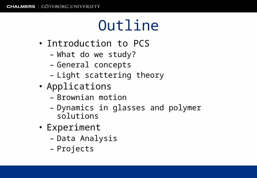
Outline• Introduction to PCS

– What do we study?– General concepts– Light scattering theory

• Applications– Brownian motion– Dynamics in glasses and polymer solutions

• Experiment– Data Analysis– Projects

General Concepts of PCS

• A dynamic light scattering technique.• Probes time variation of density and/or concentration

fluctuations.

What can we study with PCS?• Physics, chemistry, bio-physics, …

- nano-particle/colloidal solutions- liquids/liquid-glass transition- polymers/polymer solutions- gels- DNA

• Issues- particle size, radius of gyration, size of globule- diffusion of species- relaxational dynamics

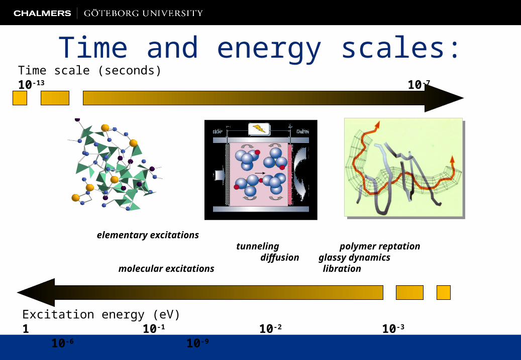
Time and energy scales:

Excitation energy (eV)1 10-1 10-2 10-3 10-6 10-9

Time scale (seconds)10-13 10-7

elementary excitationstunneling polymer reptation diffusion glassy dynamics

molecular excitations libration

Length scales:

atomic structures

organic molecules

pharmaceuticals

supermolecules

surfaces and multilayers micelles critical phenomena

proteins polymers

Length scale in nm0.01 0.1 0.3 1.0 3.0 10 30 100

50 0.5 0.05 0.005Momentum transfer (Å-1)

Spectroscopic techniques

LOG(TIME (s))-14 -10 -6 -2 2

Neutrons

Raman

Brillouin

Photon CorrelationPhoton Correlation

Dielectric

NMR

Time range of PCS

PCS covers a very large time range!

Typically: 10-8 - 103 s! => 11 decades in time!

Q-range of PCS

Q-range: ~ 10-3 Å-1

Length scales: ~ m

PCS is suitable for diffusional studies of macromolecules, such as polymers and large bio-molecules!


– What do we study?– General concepts

– Light scattering theory• Applications

– Brownian motion– Dynamics in glasses and polymer solutions


Light Scattering

Interference!

Light Scattering

Time-dependent interference!

Siegert´s relation

2

12 1)( tgtg

Einsteins theory describes the electric field correlation function,

g1(t).

PCS experiments probes the intensity correlation function

g2(t).

I(t)=E(t) E*(t)+

Gaussian approximation

Correlation function


– What do we study?– General concepts– Light scattering theory

• Applications– Brownian motion– Dynamics in glasses and polymer solutions


Brownian Motion• First observed in 1827 by the botanist Robert Brown. But Brown did not understand

what was happening. He only observed pollen grains under a microscope.

• Desaulx in 1877: "In my way of thinking the phenomenon is a result of thermal molecular motion in the liquid environment (of the particles)."

• But it was not until 1905 that the mathematical theory of Brownian motion was developed by Einstein. (It was partly for this work he received the Nobel prize 1921.)

Brownian Motion

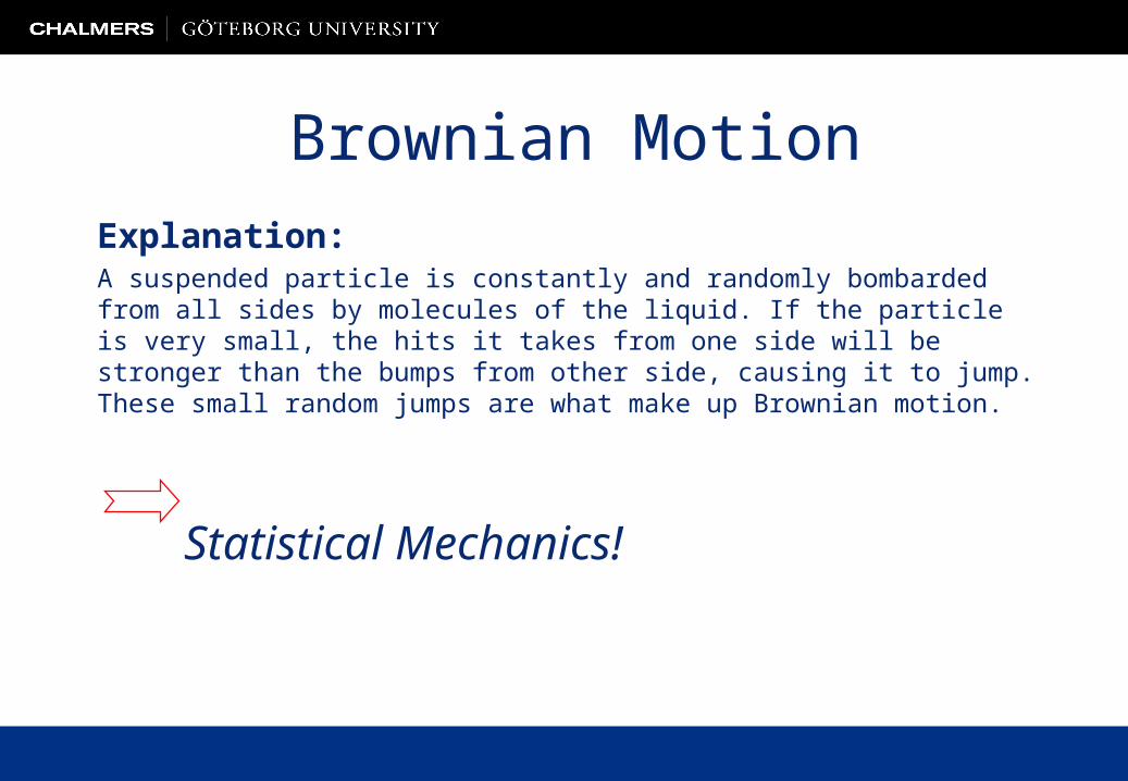
Explanation:A suspended particle is constantly and randomly bombarded from all sides by molecules of the liquid. If the particle is very small, the hits it takes from one side will be stronger than the bumps from other side, causing it to jump. These small random jumps are what make up Brownian motion.

Statistical Mechanics!

Stoke-Einsteins relation

• D diffusion constant

• T temperature

• viscosity of solvent

• r radius of particles

r

TkD B

6

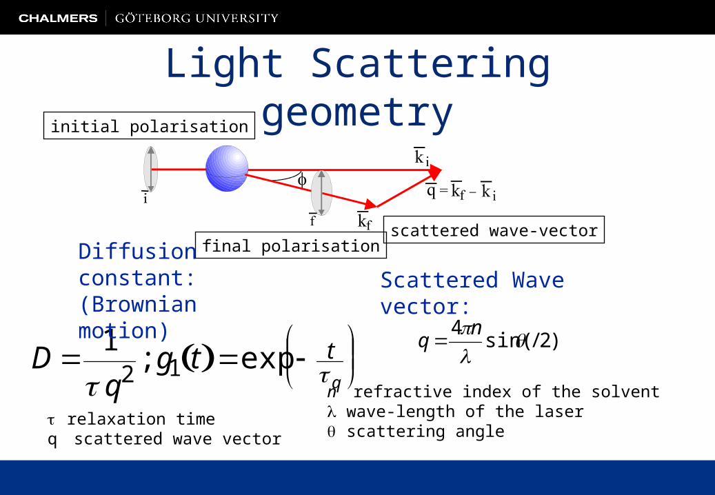
Light Scattering geometryinitial polarisation

final polarisationscattered wave-vector

)2/sin(4 n

q

Scattered Wave vector:

n refractive index of the solvent wave-length of the laser scattering angle

D 1

q2; g1 t exp t

q

Diffusion constant:(Brownian motion)

relaxation timeq scattered wave vector

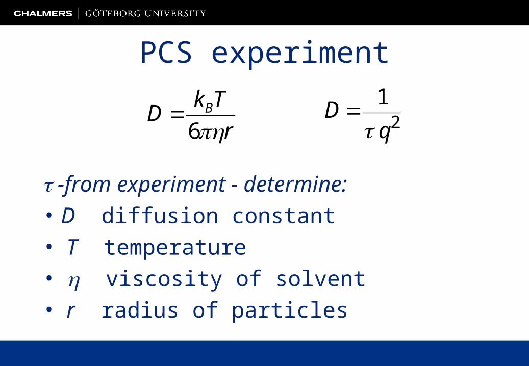
PCS experiment

-from experiment - determine:

• D diffusion constant

• T temperature

• viscosity of solvent

• r radius of particles

r

TkD B

6

D 1

q2

Research performed at Chalmers

• Glass transition dynamics

• Thin free-standing polymer films

• Dynamics in gels and polymer solutions

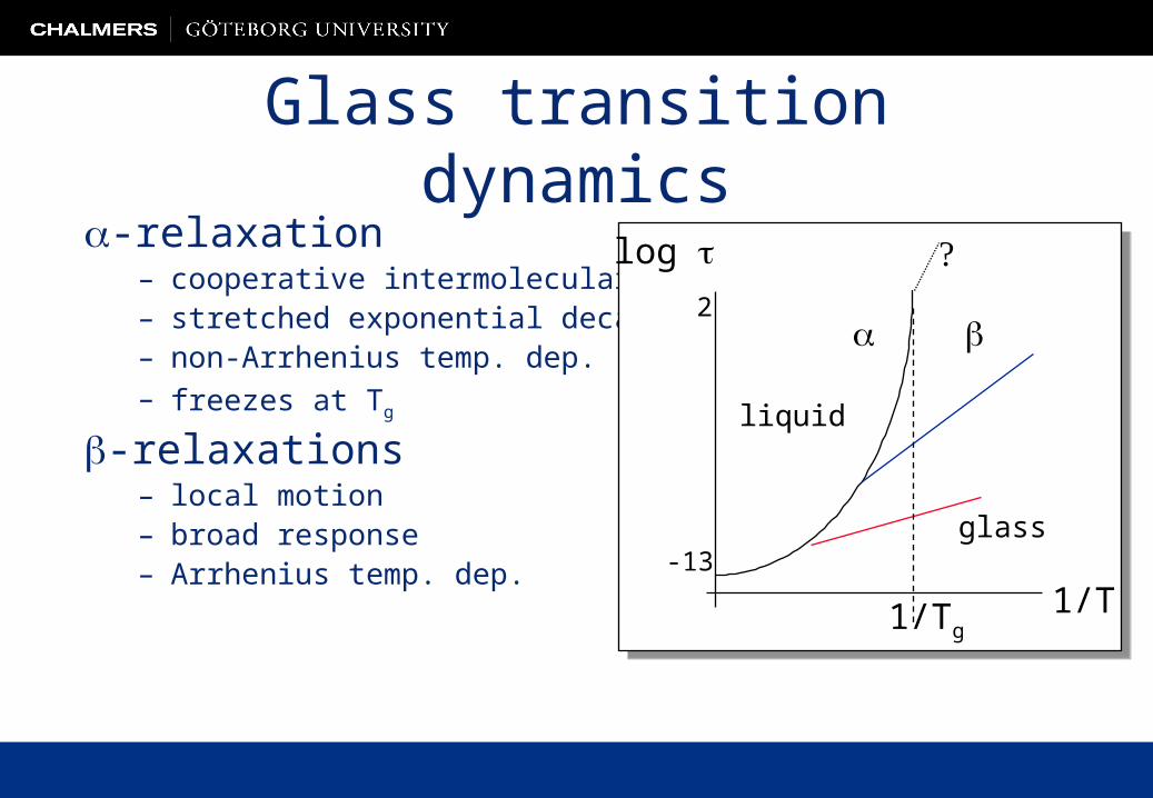
-relaxation – cooperative intermolecular motion– stretched exponential decay– non-Arrhenius temp. dep. – freezes at Tg

-relaxations– local motion– broad response – Arrhenius temp. dep.

log

1/T1/Tg

2

-13

liquid

glass

Glass transition dynamics

-relaxation – cooperative intermolecular motion– stretched exponential decay– non-Arrhenius temp. dep. – freezes at Tg

-relaxations– local motion– broad response – Arrhenius temp. dep.

log

1/T1/Tg

2

-13

liquid glass

Glass transition dynamics

PCS

fast

Poly(propylene glycol)

0

0,2

0,4

0,6

0,8

1

10-6 10-4 10-2 100 102 104

Time (s)

221 K

192 K

Temp.

Dynamics in Free-standing Polymer Films

Polystyrene200 - 500 Å

10-2 10-1 100 101 102

1,000

1,002

1,004

1,006

1,008

1,010

1200 ÅT=292 K

230 Å

g(t

)

Time (s)

10-2 10-1 100 101 102

1,000

1,002

1,004

1,006

1,008

1,010

1200 ÅT=292 K

230 Å

g(t

)

Time (s)

Dynamics of thin free-standing and supported polymer films

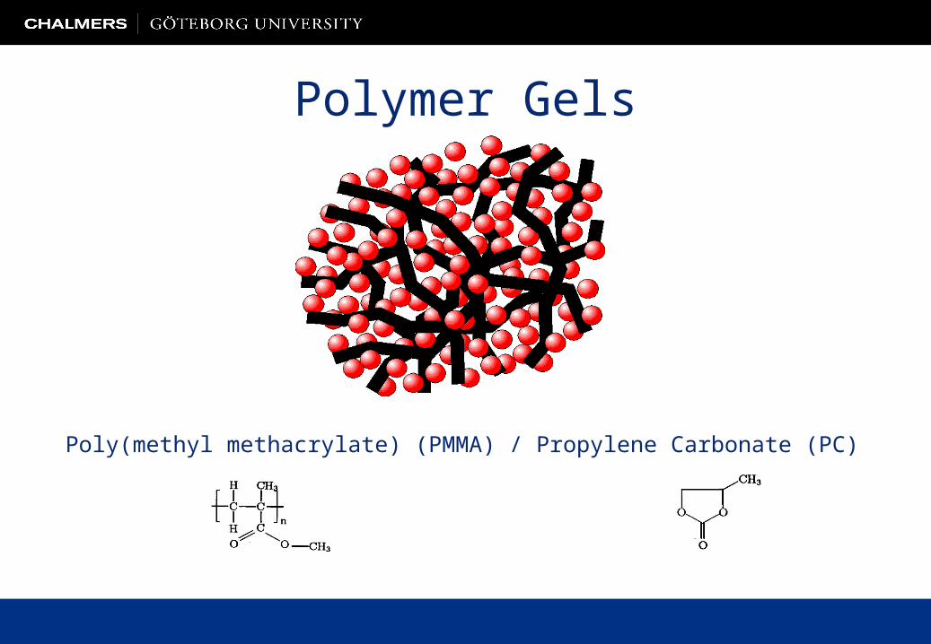
Polymer Gels

Poly(methyl methacrylate) (PMMA) / Propylene Carbonate (PC)

Dynamics in aPolymer Gel Electrolyte

Experimental Set-Up

Experimental Set-Up

Sample HolderOptics

Detector

Laser

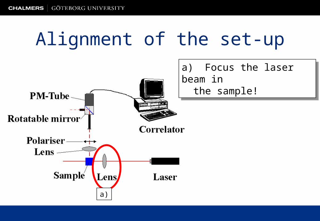
Alignment of the set-up


a) Focus the laser beam in the sample!


a)



b) Maximize the scattered light in the detector tube!


b) Maximize the scattered light in the detector tube!

b)

For your own safety:

USE THE SAFETY GOGGLES!

Experimental Data Filename.alv (binary file)

Filename.dat (ascii file)Correlator

Experimental Data Filename.alv (binary file)

Filename.dat (ascii file)

FILE Latex Spheres in Water DATE 180598 MODE REAL CORR AUTO 0 MULTIPLE TAU OFL0 NO OVERFLOW CONC .001 TEMP 293.000 PRES 1.000 ANGL 90.000 R.I. 1.330 WAVE 488.000 STC .800 NPNT 191 SAMP 343707. MONB 465494000. GENERAL 1.00, .8480350000, 137.33 2.00, .6785989000, 151.19 3.00, .5840300000, 160.21 4.00, .7849890000, 142.18 5.00, .8165120000, 139.71 6.00, .7692275000, 143.44 7.00, .8007505000, 140.93 8.00, .6510164000, 153.71 9.00, .6155530000, 157.09 10.00, .5722089000, 161.42


Correlator

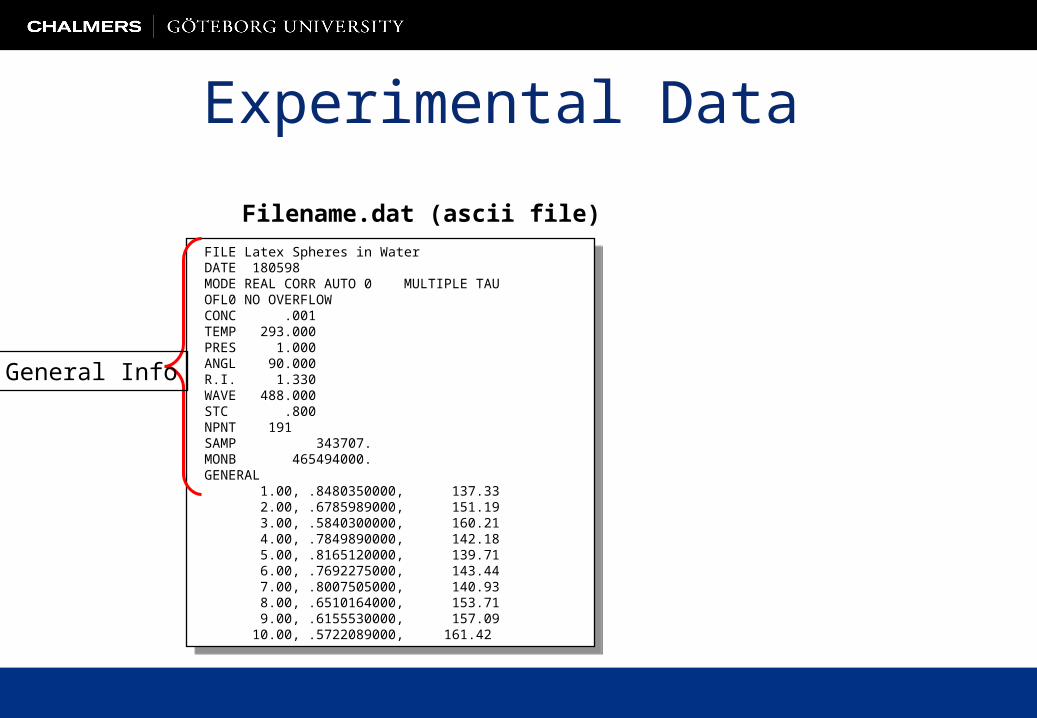
Experimental Data




General Info

Experimental Data




General Info

t = STC · X

g2(t)-1

Experimental Data




Curve-fitting: exponential function

t

Atg exp)(1

A : relaxation strength

: relaxation time

2.0

1.8

1.6

1.4

1.2

1.0

g 2(t

)

10-7

10-6

10-5

10-4

10-3

10-2

10-1

100

time (s)

Exp data Fit_Exponetial

Curve-fitting: KWW function

1.0

0.8

0.6

0.4

0.2

0.0

cor

rela

tion

-2 -1 0 1 2log ( t/ (s))

t

Atg exp)(1

A : relaxation strength

: relaxation time

: stretch parameter

Kohlrausch-Williams-Watts

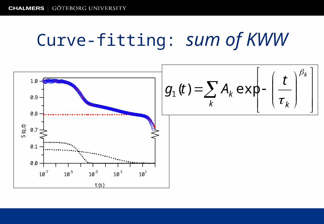
Curve-fitting: sum of KWW

0.1

0.0

S(q

,t)

10-7 10

-5 10-3 10

-1 101

t (s)

1.0

0.9

0.8

0.7

k kk

k

tAtg

exp)(1

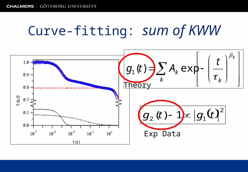
Curve-fitting: sum of KWW

0.1

0.0

S(q

,t)

10-7 10

-5 10-3 10

-1 101

t (s)

1.0

0.9

0.8

0.7

k kk

k

tAtg

exp)(1

2

12 1)( tgtg

Exp Data

Theory

Task 1: Spheres in water• Determine the size of spheres dissolved in water.

– Use PCS to determine relaxation time.

– Calculate the diffusion constant.

– Use Stoke-Einsteins relation to calculate the radius.

• Error estimation in the report!

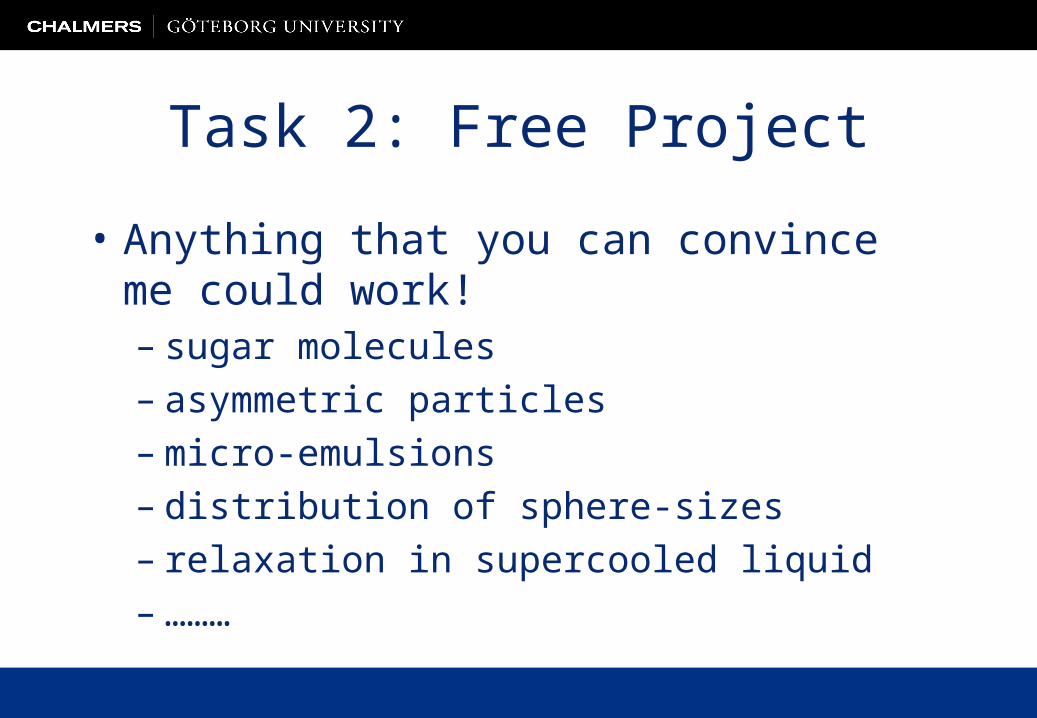
Task 2: Free Project

• Anything that you can convince me could work!– sugar molecules– asymmetric particles– micro-emulsions– distribution of sphere-sizes– relaxation in supercooled liquid– ………

What are you supposed to do? (I)Before the lab:

– Brownian motion– Stoke-Einstein relation– Correlation function– Curve-fit procedures – Project preparations

What are you supposed to do? (II)During the lab:

– Align the set-up– Determine size of spheres diluted in water– Free project

What are you supposed to do? (III)After the lab:

– Analyze data– Write report

Safety Goggles!

USE THEM!

Introduction to PHOTON CORRELATION SPECTROSCOPY. Outline Introduction to PCS –What do we study?...

Documents

Transcript of Introduction to PHOTON CORRELATION SPECTROSCOPY. Outline Introduction to PCS –What do we study?...