Introduction to Parallel Computing This document consists of two parts. The first part introduces basic concepts and issues that apply generally in discussions of parallel computing. The second part consists of several sections on various topics in parallel computing that may be read in any order. These topic sections depend on material in the first part, but do not depend on each other (unless explicitly noted otherwise).

Table  of  Contents  

Part  I:    Introduction .......................................................................................................................... 2  1   Motivation.......................................................................................................................................................................................... 2  2   Some  pairs  of  terms ....................................................................................................................................................................... 2  Part  II:    Topics................................................................................................................................... 4  A   Parallel  Speedup ............................................................................................................................................................................. 4  A.1  Introduction ........................................................................................................................................................................................4  A.2   Amdahl's  Law .................................................................................................................................................................................4  

B   Some  options  for  communication ........................................................................................................................................... 7  C   Some  issues  in  concurrency ....................................................................................................................................................... 8  D      Models  of  Parallel  Computation................................................................................................................................................. 9  

Part I: Introduction

1 Motivation Moore's "Law": an empirical observation by Intel co-founder Gordon Moore in 1965. The number of components in computer circuits had doubled each year since 1958, and Moore predicted that this doubling trend would continue for another decade. Incredibly, over four decades later, that number has continued to double each two years or less.

However, since about 2005, it has been impossible to achieve such performance improvements by making larger and faster single CPU circuits. Instead, the industry has created multi-core CPUs – single chips that contain multiple circuits for carrying out instructions (cores) per chip.

The number of cores per CPU chip is growing exponentially, in order to maintain the exponential growth curve of Moore's Law. But most software has been designed for single cores.

Therefore, CS students must learn principles of parallel computing to be prepared for careers that will require increasing understanding of how to take advantage of multi-core systems.

2 Some pairs of terms parallelism - multiple (computer) actions physically taking place at the same time concurrency - programming in order to take advantage of parallelism (or virtual parallelism)

Comments: Thus, parallelism takes place in hardware, whereas concurrency takes place in software.

Operating systems must use concurrency, since they must manage multiple processes that are abstractly executing at the same time--and can physically execute at the same time, given parallel hardware (and a capable OS).

process - the execution of a program thread - a sequence of execution within a program

Comments: Every process has at least one thread of execution, defined by that process's program counter. If there are multiple threads within a process, they share resources such as the process's memory allocation. This reduces the computational overhead for switching among threads (also called lightweight processes), and enables efficient sharing of resources (e.g., communication through shared memory locations).

sequential programming - programming for a single core concurrent programming - programming for multiple cores or multiple computers

Comments: CS students have primarily learned sequential programming in the past. These skills are still relevant, because concurrent programs ordinarily consist of sets of sequential programs intended for various cores or computers.

multi-core computing - computing with systems that provide multiple computational circuits per CPU package distributed computing - computing with systems consisting of multiple computers connected by computer network(s)

Comments: Both of these types of computing may be present in the same system (as in our MistRider and Helios clusters).

Related terms: • shared memory multiprocessing -- e.g., multi-core system, and/or multiple CPU packages in a

single computer, all sharing the same main memory • cluster -- multiple networked computers managed as a single resource and designed for working

as a unit on large computational problems • grid computing -- distributed systems at multiple locations, typically with separate

management, coordinated for working on large-scale problems • cloud computing -- computing services are accessed via networking on large, centrally managed

clusters at data centers, typically at unknown remote locations • SETI@home is another example of distributed computing.

Comments: Although multi-core processors are driving the movement to introduce more parallelism in CS courses, distributed computing concepts also merit study. For example, Intel's recently announced 48-core chip for research behaves like a distributed system with regards to interactions between its cache memories.

data parallelism - the same processing is applied to multiple subsets of a large data set in parallel task parallelism - different tasks or stages of a computation are performed in parallel

Comments: A telephone call center illustrates data parallelism: each incoming customer call (or outgoing telemarketer call) represents the services processing on different data. An assembly line (or computational pipeline) illustrates task parallelism: each stage is carried out by a different person (or processor), and all persons are working in parallel (but on different stages of different entities.)

Part II: Topics

A Parallel Speedup

A.1 Introduction The speedup of a parallel algorithm over a corresponding sequential algorithm is the ratio of the compute time for the sequential algorithm to the time for the parallel algorithm. If the speedup factor is n, then we say we have n-fold speedup. For example, if a sequential algorithm requires 10 min of compute time and a corresponding parallel algorithm requires 2 min, we say that there is 5-fold speedup.

The observed speedup depends on all implementation factors. For example, more processors often leads to more speedup; also, if other programs are running on the processors at the same time as a program implementing a parallel algorithm, those other programs may reduce the speedup. Even if a problem is embarrassingly parallel, one seldom actually obtains n-fold speedup when using n-fold processors. There are a couple of explanations for this occurrence:

• There is often overhead involved in a computation. For example, in the solar system computation, results need to be copied across the network upon every iteration. This communication is essential to the algorithm, yet the time spend on this communication does not directly compute more solutions to the n-body problem.

In general, communication costs are frequent contributors to overhead. The processing time to schedule and dispatch processes also leads to overhead.

• trues occur when a process must wait for another process to deliver computing resources. For example, after each computer in the solar system computation delivers the results of its iteration, it must wait to receive the updated values for other planets before beginning its next iteration.

• Some parts of a computation may be inherently sequential. In the polar ice example, only the matrix computation was parallelized, and other parts gained in performance only because they were performed on faster hardware and software (on a single computer)

On rare occasions, using n processors may lead to more than an n-fold speedup. For example, if a computation involves a large data set that does not fit into the main memory of a single computer, but does fit into the collective main memories of n computers, and if an embarrassingly parallel implementation requires only proportional portions of the data, then the parallel computation involving n computers may run more than n times as fast because disk accesses can be replaced by main-memory accesses.

Replacing main-memory accesses by cache accesses could have a similar effect. Also, parallel pruning in a backtracking algorithm could make it possible for one process to avoid an unnecessary computation because of the prior work of another process.

A.2 Amdahl's Law Amdahl's Law is a formula for estimating the maximum speedup from an algorithm that is part sequential and part parallel. The search for 2k-digit primes illustrates this kind of problem: First, we

create a list of all k-digit primes, using a sequential sieve strategy; then we check 2k-digit random numbers in parallel until we find a prime.

The Amdahl's Law formula is

• P is the time proportion of the algorithm that can be parallelized.

• S is the speedup factor for that portion of the algorithm due to parallelization.

For example, suppose that we use our strategy to search for primes using 4 processors, and that 90% of the running time is spent checking 2k-digit random numbers for primality (after an initial 10% of the running time computing a list of k-digit primes). Then P = .90 and S = 4 (for 4-fold speedup). According to Amdahl's Law,

This estimates that we will obtain about 3-fold speedup by using 4-fold parallelism.

Note: • Amdahl's Law computes the overall speedup, taking into account that the sequential portion of

the algorithm has no speedup, but the parallel portion of the algorithm has speedup S.

• It may seem surprising that we obtain only 3-fold overall speedup when 90% of the algorithm achieves 4-fold speedup. This is a lesson of Amdahl's Law: the non-parallelizable portion of the algorithm has a disproportionate effect on the overall speedup.

• A non-computational example may help explain this effect. Suppose that a team of four students is producing a report, together with an executive summary, where the main body of the report requires 8 hours to write, and the executive summary requires one hour to write and must have a single author (representing a sequential task). If only one person wrote the entire report, it would require 9 hours. But if the four students each write 1/4 of the body of the report (2 hours, in 4-fold parallelism), then one student writes the summary, then the elapsed time would be 3 hours---for a 3-fold overall speedup. The sequential portion of the task has a disproportionate effect because the other three students have nothing to do during that portion of the task.

A short computation shows why Amdahl's Law is true.

• Let Ts be the compute time without parallelism, and Tp the compute time with parallelism. Then, the speedup due to parallelism is

• The value P in Amdahl's Law is the proportion of Ts that can be parallelized, a number between 0 and 1. Then, the proportion of Ts that cannot be parallelized is 1-P.

• This means that

• We conclude that

B Some options for communication In simple data parallelism, it may not be necessary for parallel computations to share data with each other during the executions of their programs. However, most other forms of concurrency require communication between parallel computations. Here are three options for communicating between various processes/threads running in parallel.

1. message passing - communicating with basic operations send and receive to transmit information from one computation to another.

2. shared memory - communicating by reading and writing from local memory locations that are accessible by multiple computations

3. distributed memory - some parallel computing systems provide a service for sharing memory locations on a remote computer system, enabling non-local reads and writes to a memory location for communication.

Comments: For distributed systems, message passing and distributed memory (if available) may be used. All three approaches may be used in concurrent programming in multi-core parallelism. However, shared (local) memory access typically offers an attractive speed advantage over message passing and remote distributed memory access

When multiple processes or threads have both read and write access to a memory location, there is potential for a race condition, in which the correct behavior of the system depends on timing. (Example: filling a shared array, with algorithms for accessing and updating a variable nextindex.)

• resource - a hardware or software entity that can be allocated to a process by an operating system Comments: A memory location is an example of a (OS) resource; other examples are: files; open files; network connections; disks; GPUs; print queue entries. Race conditions may occur around the handling of any OS resource, not just memory locations.

• In the study of Operating Systems, inter-process communication (IPC) strategies are used to avoid problems such as race conditions. Message passing is an example of an IPC strategy. (Example: solving the array access problem with message passing.)

• Message passing can be used to solve IPC problems in a distributed system. Other common IPC strategies (semaphores, monitors, etc.) are designed for a single (possibly multi-core) computer.

C Some issues in concurrency We will use the Hadoop implementation of map-reduce for clusters as a running example.

Fault tolerance is the capacity of a computing system to continue to satisfy its spec in the presence of faults (causes of error)

Comments: With more parallel computing components and more interactions between them, more faults become possible. Also, in large computations, the cost of restarting a computation may become greater. Thus, fault tolerance becomes more important and more challenging as one increases the use of parallelism. Systems (such as map-reduce) that automatically provide for fault tolerance help programmers of parallel systems become more productive.

Mutually exclusive access to shared resources means that at most one computation (process or thread) can access a resource (such as a shared memory location) at a time. This is one of the requirements for correct IPC. One approach to mutually exclusive access is locking, in which a mechanism is provided for one computation to acquire a "lock" that only one computation may hold at any given time. A computation possessing the lock may then use that lock's resource without fear of interference by another process, then release the lock when done.

Comments: Designing computationally correct locking systems and using them correctly for IPC can often be quite tricky.

Scheduling means assigning computations (processes or threads) to processors (cores, distributed computers, etc.) according to time. For example, in map-reduce computing, we mapper processes are scheduled to particular cluster nodes having the necessary local data; they are rescheduled in the case of faults; reducers are scheduled at a later time.

D Models of Parallel Computation

Types of parallel computers, or platforms Until 2004, when the first dual core processors for entry-level computer systems were sold, all computers that most individuals used on a regular basis contained one central processing unit (CPU). These computers were classic von Neuman machines, where single instructions executed sequentially. Some of these instructions can read or write values to random access memory (RAM) connected to the CPU. These machines are said to follow the traditional RAM model of computation, where a single processor has read and write (RW) access to memory. Today, even the next generation of netbooks and mobile phones, along with our current laptops and desktop machines, have dual core processors, containing two ‘cores’ capable of executing instructions on one CPU chip. High-end desktop workstations and servers now have chips with more cores (typicaly 4 or 8), which leads to the general term multicore to refer to these types of CPUs. This trend of increasing cores will continue for the foreseeable future- the era of single processors is gone. In addition to the trend of individual machines containing multiple processing units, there is a growing trend towards harnessing the power of multiple machines together to solve ever larger computational and data processing problems. Since the early to mid 1980’s, many expensive computers containing multiple processors were built to solve the world’s most challenging computational problems. Since the mid-1990’s, people have built clusters of commodity PCs that are networked together and act as a single computer with multiple processors (which could be multicore themselves). This type of cluster of computers is often referred to as a beowulf cluster, for the first of these that was built and published. Major Internet software companies such as Google, Yahoo, and Microsoft now employ massive data centers containing thousands of computers to handle very large data processing tasks and search requests from millions of users. Portions of these data centers can now be rented out at reasonable prices from Amazon Web Services, making it possible for those of us who can write parallel programs to harness the power of computers in ‘the cloud’- out on the Internet away from our own physical location. Thus, in fairly common use today we have these major classes of parallel computing platforms:

• multicore with shared memory, • clusters of computers that can be used together, and • large data centers in the cloud.

In addition, in the past there were many types of multiprocessor computers built for parallel processing. We draw on the research work conducted using these computers during the 1980’s and 1990’s to explain the following theoretical framework to describe models of parallel computing.

Theoretical Parallel Computing Models The advent of these various types of computing platforms adds complexity to how we consider the operation of these machines. For simplicity, we will loosely use the term ‘processor’ in the following discussion to refer to each possible processing unit that can execute instructions in the three major types of platforms described above (you will likely see this term being used differently in future hardware design or operating systems courses). The memory might be shared by all processors, some of the processors, or none (each has its own assigned memory). Each processor may be

capable of sending data to every other processor, but it may not. We need to define a framework to describe these various possibilities as different types of computing models. The type of computing model will dictate whether certain algorithms will be effective at speeding up an equivalent task on a single sequential RAM computer.

The PRAM model The sequential RAM computer with one processor differs from parallel computing platforms not only because there are multiple processing units, but also because they can vary in how available memory is accessed. When considering algorithms for parallel platforms, it is useful to consider an abstract, theoretically ideal computing model called a Parallel Random Access Machine, or PRAM. In such a machine, a single program runs on all processors, each of which has access to a main memory that is shared among them, as in Figure 1.

Figure 1. The PRAM model. (Image taken from http://www.mesham.com/article/Communication) A PRAM machine with large numbers of processors has not been built in practice, but the model is useful when designing algorithms because we can reason about the complexity of those algorithms. The common multicore machines available today can be considered to be PRAM, but have a low number of processors (n in Figure 1). Note that the hardware involved to enable all processors to have access to memory is difficult to build so that it is fast, which is why we don’t yet have PRAM machines with many processors and large amounts of memory (This will be clearer when you’ve take a hardware design or computer organization course.) Having many processing units, each running a program simultaneously, increases the complexity about how they coordinate to access memory. In this case, more than one processor may want to read from or write to the same memory location at the same time. In the theoretical PRAM model, it is useful for us to consider the following three possible strategies for handling these simultaneous attempts to access a data element in memory:

4. Exclusive Read, Exclusive Write (EREW). Only one processor at a time can read a memory value and only one processor at a time can write a memory value.

5. Concurrent Read, Exclusive Write (CREW). Many processors can read a data value at one time, but only one processor at a time can write a memory value.

6. Concurrent Read, Concurrent Write (CRCW). Many processors can read a data value at one time, and many processors can write a data value at one time.

You may be wondering what we mean by a memory value. We could consider various granularities: it might be a whole array of data, such as integers, or it might be the individual integers themselves. In practice, this can vary for various types of hardware. For simplicity, we will assume that one memory value is one data value, such as an integer, a floating point number, or a character- these are what each processor can access. With each of these memory access models, we also need to consider what order the reads and writes will occur in. As you consider parallel algorithms for various tasks, it may become necessary to reason about which process of the more than one that require access to a data item will be chosen to go first. You want avoid solutions where the order of reads and writes will make a difference in the final result, but it may become important to specify ordering.

For concurrent reads (CR) between processors, all will get the same result and memory is not changed, so there is not a conflict at that single step that would cause your solution to be incorrect, unless you’ve devised an incorrect solution. Exclusive write (EW) typically means that your code should be designed so that only one processor is writing a data value to one memory location at one execution step. Likewise, exclusive read (ER) usually means that your code should be written such that only one processor reads a data value at one step. For EW and ER, a runtime error in your code would result if more than one processor attempted to read or write to the same data value at a certain step. Concurrent writes could be handled in a variety of ways; one of the more common approaches is to state that a higher (or lower) processor number goes first, thus giving it priority. This concurrent write case is the hardest to design algorithms for. Luckily, it is not yet achieved in practice, so we won’t spend time considering it..

All of this discussion about the PRAM model of a parallel machine leads us to one more important point that you may be wondering about: when we have a program running on multiple processors, just which step is running on each processor at any point in time? As you might guess, the answer once again in practice depends on the type of machine. In the PRAM model we have two main types of program step execution on data:

• Multiple Instruction, Multiple Data (MIMD): each processor is stepping through the program instructions independently of the other processors, and each could be working on different data values.

• Single Instruction, Multiple Data (SIMD): each processor is on the same instruction at any time, but but each is working on a separate data value.

For the rest of this discussion, we will assume that our PRAM machine is a MIMD machine,

Stop and Consider this: If we are assuming a SIMD PRAM machine, do we need to worry about which data access pattern (EREW, CREW, or CRCW) we have?

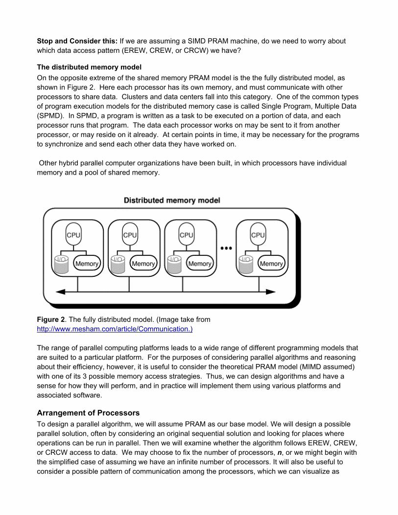
The distributed memory model On the opposite extreme of the shared memory PRAM model is the the fully distributed model, as shown in Figure 2. Here each processor has its own memory, and must communicate with other processors to share data. Clusters and data centers fall into this category. One of the common types of program execution models for the distributed memory case is called Single Program, Multiple Data (SPMD). In SPMD, a program is written as a task to be executed on a portion of data, and each processor runs that program. The data each processor works on may be sent to it from another processor, or may reside on it already. At certain points in time, it may be necessary for the programs to synchronize and send each other data they have worked on. Other hybrid parallel computer organizations have been built, in which processors have individual memory and a pool of shared memory.

Figure 2. The fully distributed model. (Image take from http://www.mesham.com/article/Communication.) The range of parallel computing platforms leads to a wide range of different programming models that are suited to a particular platform. For the purposes of considering parallel algorithms and reasoning about their efficiency, however, it is useful to consider the theoretical PRAM model (MIMD assumed) with one of its 3 possible memory access strategies. Thus, we can design algorithms and have a sense for how they will perform, and in practice will implement them using various platforms and associated software.

Arrangement of Processors To design a parallel algorithm, we will assume PRAM as our base model. We will design a possible parallel solution, often by considering an original sequential solution and looking for places where operations can be run in parallel. Then we will examine whether the algorithm follows EREW, CREW, or CRCW access to data. We may choose to fix the number of processors, n, or we might begin with the simplified case of assuming we have an infinite number of processors. It will also be useful to consider a possible pattern of communication among the processors, which we can visualize as

placing them in a particular arrangement. The simplest arrangements are shown in Figure 3: a linear array (which can be extended to a ring by connecting P1 to Pn), a mesh, or a binary tree.

Figure 3. Simple, yet useful arrangements of processors to consider when designing parallel algorithms.