Introduction to Parallel Computing - par.tuwien.ac.at · WS17/18 ©Jesper Larsson Träff...

©Jesper Larsson TräffWS17/18

Introduction to Parallel ComputingHigh-Performance Computing. Prefix sums

Jesper Larsson Trä[email protected]

TU WienParallel Computing

mailto:[email protected]


Applied parallel computing: High-Performance Computing (HPC)

• Solving the problems faster• Solving larger problems• Solving problems more cheaply (less energy)

HPC:Solving given (scientific, computationally and memory intensive) problems on real (parallel) machines

• Which problems? (not this lecture)• Which real parallel machines (not really this lecture)?• How, which parallel computing techniques (some)?

See HPC Master lecture


High-Performance Computing/Scientific Computing

Focus on problems:Important, computation-intensive problems needing to be solved

• Anything goes attitude… (parallel computing to the rescue, not per se)

• Significant investments (politics) in new machines suited to solving these problems

90ties, early 2000: HPC (only) niche for parallel computing

Focus on machines:FLOPS (Floating Point OPerations per Second)


Scientific Computing/High-Performance Computing Problems

• “Grand challenge problems”: Climate, global warming• Engineering: CAD, simulations (fluid dynamics)• Physics: Cosmology, particle physics, quantum physics, string

theory, …• Biology, chemistry: Protein folding, genetics

• Data mining („Big Data“)

• Drug design, screening• Security, military??? Who knows? NSA-decryption?

Both politically/societally/commercially and scientifically motivated problems

Not this lecture


Intel iPSC

IBM SP

INMOS Transputer

MasPar

Thinking Machines CM2

Thinking Machines CM-5

1985 1992 20061979

PRAM: Parallel RAM

SB-PRAM

Big surge in general purpose parallel systems ca. 1987-1992

Big surge in theory: parallel algorithmicsca. 1980-1993

Some recent history: Parallel systems and parallel theory

High-Performance Computing

“Practice”

“Theory”activity

acti

vity


MasPar (1987-1996) MP2

Thinking Machines (1982-94) CM2, CM5

MasPar, CM2:SIMD machinesCM5: MIMD machine


“Top” HPC systems 1993-2000 (from www.top500.org)

http://www.top500.org/


• Politically motivated; answer to Japan’s 5th generation project (massively parallel computing based on logic programming)

• “Grand challenge problems” (CFD, Quantum, Fusion, Weather/climate, Symbolic computation)

• Abundant military funding (R. Reagan, 1911-2004: Star Wars, …)

• Some belief that sequential computing was approaching its limits

• A good model for theory: The PRAM (circuits, etc.)

• …

Surge in parallel computing late 80ties, early 90ties

Still holds, NSA, …

Exponential improvement stopped ca. 2005

Is lacking, PRAM not embraced

Now (2016)

Still grand challenges


Intel iPSC

IBM SP

INMOS Transputer

MasPar

Thinking Machines CM2

Thinking Machines CM-5

1985 1992 20061979

PRAM: Parallel RAM

SB-PRAM

Parallel computing/algorithmicsdisappeared from mainstream CS

90ties: Companies went out of business, systems disappeared

No parallel algorithmics

Still commerciallytough

The lost decade: A lost generation

activity

acti

vity


Recent history (2010) :

SiCortex (2003-09): distributed memory MIMD, Kautz-network

2010: Difficult to build (and survive commercially) “best”, real parallel computers with

• Custom processors• Custom memory• Custom communication

network


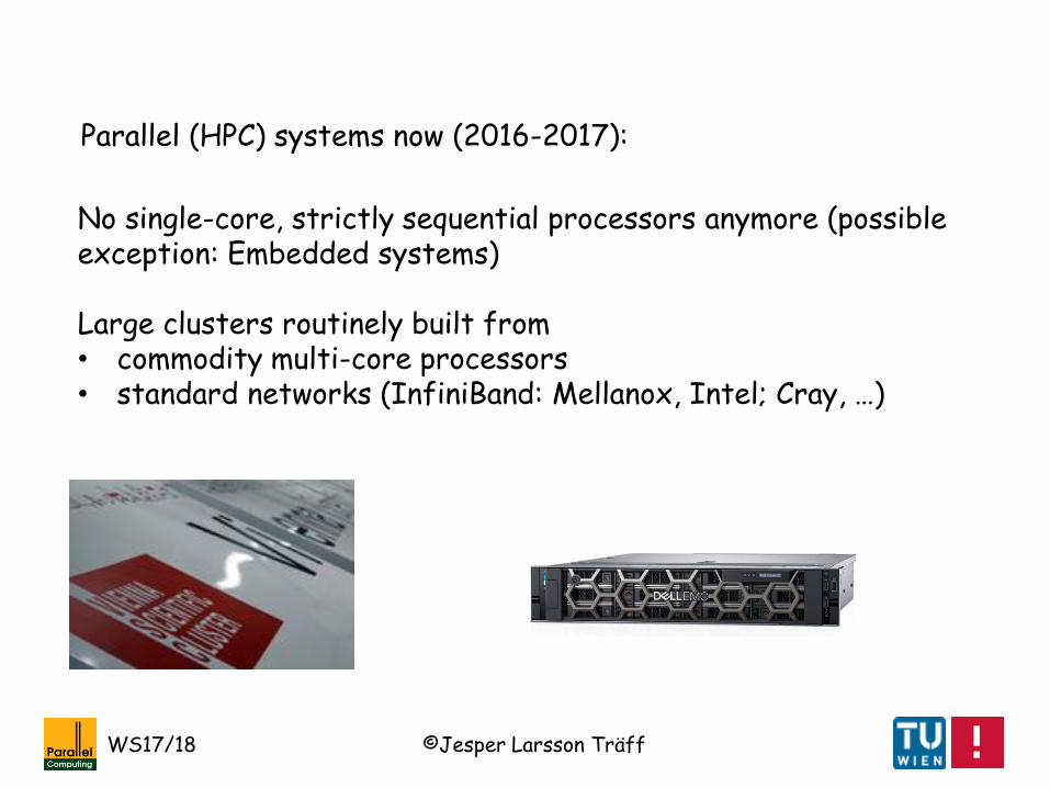
Parallel (HPC) systems now (2016-2017):

No single-core, strictly sequential processors anymore (possible exception: Embedded systems)

Large clusters routinely built from• commodity multi-core processors• standard networks (InfiniBand: Mellanox, Intel; Cray, …)


Recap: Processor developments 1970-2010

Raw clockspeedleveledout

Perf/clockleveled out

Limits to power consumption

Number oftransistors still (exponentially) growing

Kunle Olukotun (Stanford), ca. 2010


Moore‘s „Law“ (popular version):Sequential processor performance doubles every 18 months

Gordon Moore: Cramming more components onto integratedcircuits. Electronics, 38(8), 114-117, 1965

Exponential growth in performance often referred to as

Moore’s “Law” is (only) an empirical observation/extrapolation.

Not to be confused with physical “law of nature” or “mathematical law” (e.g. Amdahl)


Moore‘s „law“ (≈ „free lunch“) effectively killed parallel computing in the 90ties:

Parallel computers, typically relying on processor technologies a few generations old, and taking years to develop and market, could not keep up

To increase performance by an order of magnitude (factor 10 orso), just wait 3 processor generations = 4.5 to 6 years („freelunch“) Steep increase in performance/€

Performance/€ ??

Parallel computers were not commercially viable in the 90ties

This has changed


Moore‘s „Law“ (what Moore originally observed):Transistor counts double roughly every 12 months (1965 version); every 24 months (1974 version)

What are all thesetransistors used for?

Gordon Moore: Cramming more components onto integratedcircuits. Electronics, 38(8), 114-117, 1965

So few transistors (in the thousands) needed for full microprocessor

Computer Architecture: What’s the best way to use transistors


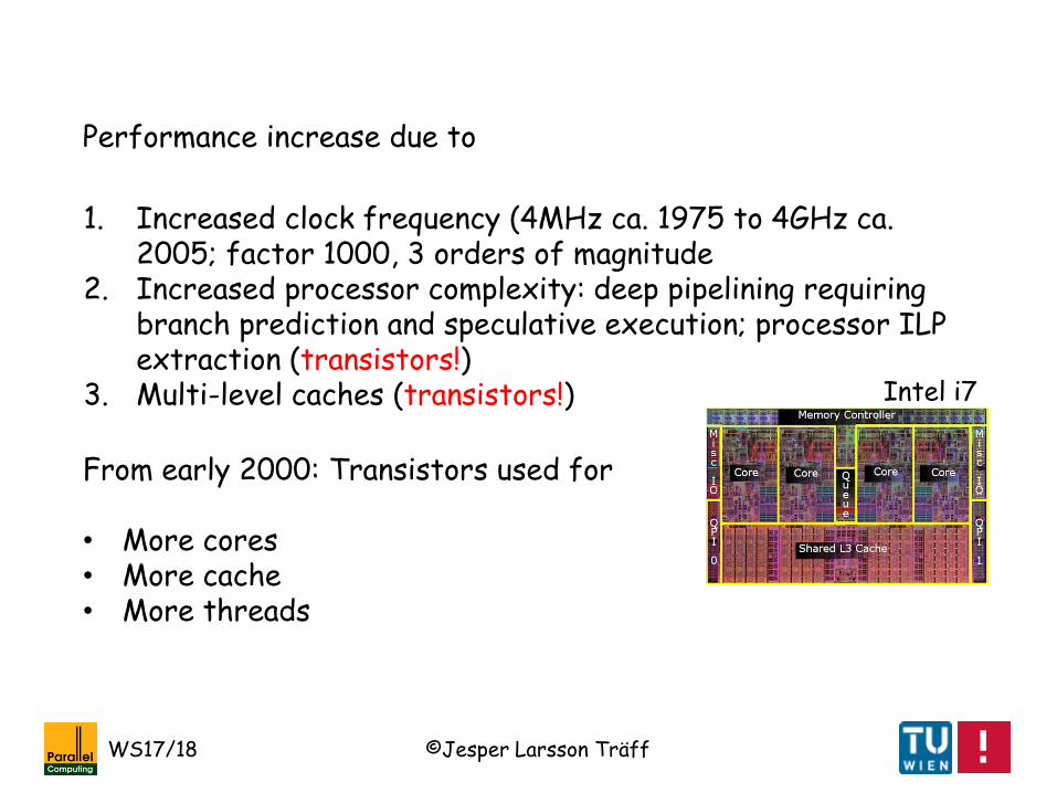
Performance increase due to

1. Increased clock frequency (4MHz ca. 1975 to 4GHz ca. 2005; factor 1000, 3 orders of magnitude

2. Increased processor complexity: deep pipelining requiring branch prediction and speculative execution; processor ILP extraction (transistors!)

3. Multi-level caches (transistors!) Intel i7

From early 2000: Transistors used for

• More cores• More cache• More threads


HPC systems: Top500 list

Ranking of the 500 “most powerful” HPC systems in the world:

• System “peak performance” reported by running H(igh)P(erformance)LINPACK benchmark

• List updated twice yearly, June (ISC Conference, Germany), and November (Supercomputing Conference, USA), since 1993

• Rules for how to submit an entry (accuracy, algorithms)

Criticism:• Is performance ranking based on a single benchmark

indicative?• Is the benchmark capturing most relevant system or problem

characteristics?• Is the benchmarking transparent enough?• Has turned into decision making criterion


Nevertheless…

The Top500 list: Interesting and sometimes valuable source of information about HPC system design since 1993: Trends in HPC/parallel computer architecture

HPLINPACK benchmark (evolved from early linear algebra packages): Solve dense system of n linear equations with n unknowns: Given nxn matrix A, n-element vector b, solve

Ax = b

Solution by LU- factorization, can use BLAS etc., but operation count must be 2/3n3+O(n2) (“Strassen” etc. excluded); all kinds of optimizations (algorithm engineering) allowed

For each new system: Significant amount of work goes into optimizing and running HPLINPACK


Top system performance well over 5 PFLOPS (1015

FLOPS)

From www.top500.org, June 2011, peak LINPACK performance

Metric is FLOPS: Floating Point Operations per Second

Smooth, Moore-like exponential performance increase



June 2016: Peak LINPACK performance over 93PFLOPS

• Cumulated performance, all 500 systems

• #1 system• #500 system


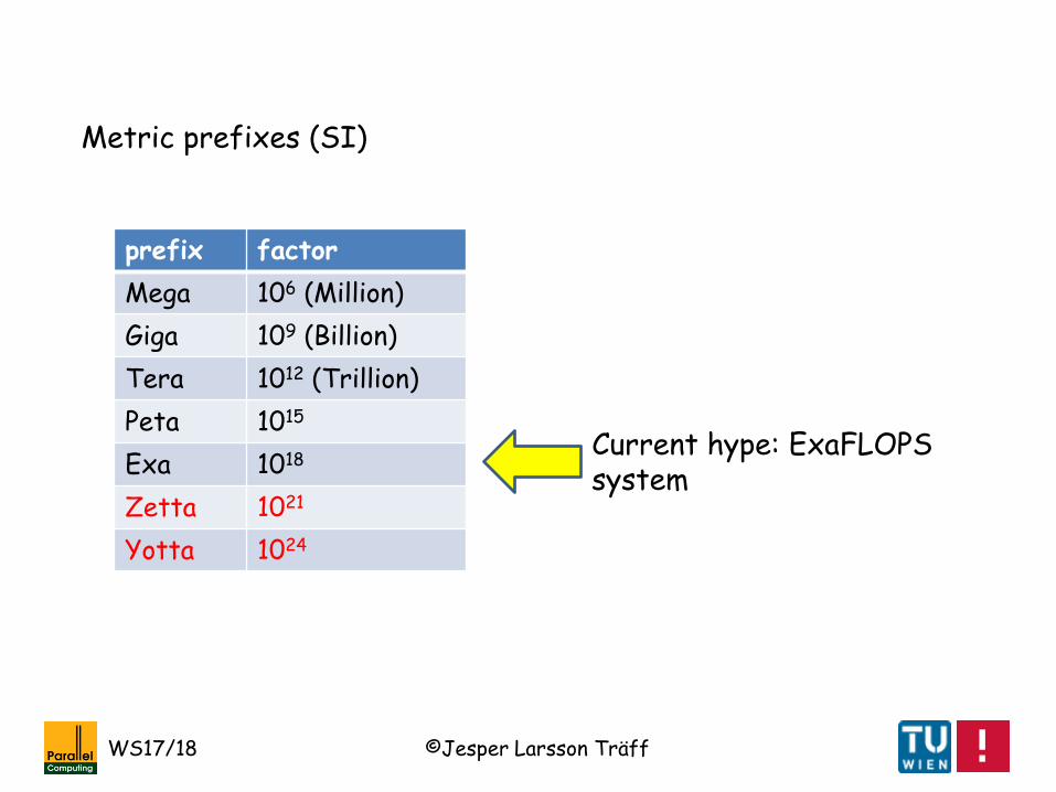
prefix factor

Mega 106 (Million)

Giga 109 (Billion)

Tera 1012 (Trillion)

Peta 1015

Exa 1018

Zetta 1021

Yotta 1024

Metric prefixes (SI)

Current hype: ExaFLOPSsystem


# Organization System Manufac Country Cores Rmax Rpeak

1

RIKEN Advanced

Institute for

Computational Science

K computer,

SPARC64 VIIIfx

Tofu interconnect Fujitsu Japan 548352 8162000 8773630

2

National

Supercomputing Center

Tianjin

Intel X5670,

NVIDIA GPU, NUDT China 186368 2566000 4701000

3

DOE/SC/Oak Ridge

National Laboratory

Cray XT5-HE

Opteron 6-core Cray Inc. USA 224162 1759000 2331000

4

National

Supercomputing Centre

Shenzhen

Intel X5650,

NVidia Tesla GPUDawning China 120640 1271000 2984300

5

GSIC Center, Tokyo

Institute of Technology

Xeon X5670,

Nvidia GPU NEC/HP Japan 73278 1192000 2287630

6DOE/NNSA/LANL/SNL Cray XE6 Cray Inc. USA 142272 1110000 1365810

7

NASA/Ames Research

Center/NAS

SGI Altix Xeon

Infiniband SGI USA 111104 1088000 1315330

8DOE/SC/LBNL/NERSC Cray XE6 Cray Inc. USA 153408 1054000 1288630

9

Commissariat a l'Energie

Atomique Bull Bull SA France 138368 1050000 1254550

10DOE/NNSA/LANL

PowerX Cell 8i

Opteron

Infiniband IBM USA 122400 1042000 1375780

June 2011


# Organization System Manufac Country Cores Rmax Rpeak

…

56

TU Wien, Uni Wien,

BOKU

Opteron,

Infiniband Megware Austria 20700135600 185010

…

Rmax (=LINPACK), Rpeak (=Hardware): Measured in GFLOPS

VSC-2: Vienna Scientific Cluster

June 2016: VSC-3

# cores Rmax Rpeak Power

169VSCAustria

Intel Xeon E5-2650v2 8C 2.6GHz, Intel TrueScaleInfiniband

32,768 596.0 681.6 450

In TFLOPS


June 2011

NEC Earth Simulator: 2002-2004

NEC Earth Simulator2, 2009


Some trends from www.top500.org

• Since ca. 1995 no single-processor system on list

• 2013: Most powerful systems have well over 1,000,000 cores

• 2013: Highest end dominated by torus network (Cray, IBM, Fujitsu): large diameter and low bisection

• Since early 2000: Clusters of shared-memory nodes

• Few specific HPC processor architectures (no vector computers)

• Hybrid/heterogeneous computing: accelerators (Nvidia GPU, Radeon GPU, Cell, Intel Xeon Phi/MIC…)



Supercomputer performance development obeys Moore‘s law: Use Top500 data for prediction

2013:ProjectedExascale(1018 FLOPS) ca. 2018


2016 prediction

2016:ProjectedExascale (1018

FLOPS) ca. 2020?


Is Top500 evidence/support for Moore‘s „law“?

What is an empirical “law”?• Observation• Extrapolation• Forecast• Prediction• Self-fulfilling prophecy• (Political) dictate

“Law’s” that (just) summarize empirical observations can sometimes be externally influenced.

“Moore’s law”: Not at all a law of nature, what it projects can (and is) very well be influenced externally

Contrast: “Amdahl’s Law”, a simple mathematical fact

Contrast: Law of nature, some notion of necessity, explanatory power (why?), empirically falsifiable/supportable


Peter Hofstee, IBM Cell co-designer

„…a self-fulfilling prophecy… nobody can afford to put a processor or machine on the market that does not followit“, HPPC 2009

Decommisioned 31.3.2013

The “Moore’s law” like behavior and projection of the Top500 list has inflicted HPC: Sponsors want to see their system high on the list (#1).

This explains dubious utility of some recent systems

Not harmless:HPC systems cost time and money


HPC: Hardware-oriented notion of efficiency

HPC Efficiency:Ratio of FLOPS achieved by the application to “theoretical peak-rate”

Caution:• Not always well-defined what “theoretical peak-rate” is• Measuring FLOPS: Inferior algorithm may be more “efficient”

than otherwise preferable algorithm• Top500 and elsewhere in HPC

Measures how well hardware/system capabilities are actually used by the given application

Contrast: Our algorithm-oriented notion of efficiency (TSeq(n)/p)/Tpar(p,n)


FLOPS: Number of Floating Point OPerations per Second

• In early microprocessor history, floating point operations were expensive (sometimes done by separate FPU)

• In many scientific problems, floating point operations is where the work is

Optimistic upper bound on application performance:Total number of floating point operations that a (multi-core/parallel) processor might be capable of carrying out in the best case where all floating point units operate at the same time and suffer no memory or other delays

HPC system FLOPS ≈nodes*cores/node*clock/core*FPinstructions/clock


Refined hardware performance model

Samuel Williams, Andrew Waterman, David A. Patterson: Roofline: an insightful visual performance model for multicorearchitectures. Commun. ACM (CACM) 52(4):65-76 (2009)

Georg Ofenbeck, Ruedi Steinmann, Victoria Caparros, Daniele G. Spampinato, Markus Püschel: Applying the roofline model. ISPASS 2014:76-85JeeWhan Choi, Daniel Bedard, Robert J. Fowler, Richard W. Vuduc: A Roofline Model of Energy. IPDPS 2013:661-672

Roofline:Judging application performance relative to specific, measured hardware capabilities, including memory bandwidth. Goal: How close is application performance to hardware upper bound?

More in HPC Master lecture


Other HPC benchmarks

HPC Challenge (HPCC) benchmarks: Suite of more versatile benchmarks in the vein of HPLINPACK. HPCC suite consists of• HPLINPACK• DGEMM (level 3 BLAS matrix-matrix multiply)• STREAM memory bandwidth and arithmetic core

performance• PTRANS matrix transpose (all-to-all)• Random access benchmark• FFT• Communication latency and bandwidth for certain patterns

www.green500.org: Measures energy efficiency, FLOPS/Wattwww.graph500.org: Performance measure based on BFS-like graph search; irregular, non-numerical application kernel

http://www.green500.org/

http://www.graph500.org/


Speedup in HPC

Speedup as theoretical measure:Ratio of (analyzed) performance (time, memory) of parallel algorithm to (analyzed) performance of best possible sequential algorithm in chosen computational model

Sp(n) = Tseq(n)/Tpar(p,n)

Assumptions:Same computational model for sequential and parallel algorithm; constants often ignored, asymptotic performance (large n and large p)

Superlinear speedup not possible, speedup at most p (perfect), under stated assumption


Speedup as empirical measure:Ratio of measured performance (time, memory, energy) of parallel implementation to measured performance of best known available, sequential implementation in given system

Sequential and parallel system may simply differ.What is speedup when using accelerators (GPU, MIC, …)?

Factors:• System (architecture, hardware, software)• Implementation (language, libraries, model)• Algorithm• Measurement, reproducibility (Top500 HPC systems

sometimes “once-in-a-lifetime”)


Can Tseq(n) be known?

As p grows (HPC systems in the order of 100,000 to 1,000,000 cores) it may not be possible to measure Tseq(n): For problems where input of size n is split evenly across p processors, n might be too large to fit into the memory of a single processor, so no Tseq(n) for such n

Possible way out: Exploit weak-scaling properties

Observation:Strongly scaling implementation is also weakly scaling (with constant iso-efficiency function)


Approach 1:

• Measure Sp(n) = Tseq(p,n)/Tpar(p,n) for 1≤p<p0, and some fixed n, n≤n0

• Measure Sp(n) = Tseq(p,n)/Tpar(p,n) for p0≤p<p1, and some other, larger fixed n, n0≤n<p0n0

• …

Examples: p0=1000, p1=10,000, … or p0 = number of cores per compute node (see later), p1 = number of nodes per rack (see later), or, …

Approach 2:

Choose n (fitting on one processor), compare Tpar(1,n) to Tpar(p,pn)


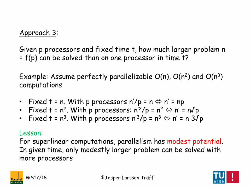
Approach 3:

Given p processors and fixed time t, how much larger problem n = f(p) can be solved than on one processor in time t?

Example: Assume perfectly parallelizable O(n), O(n2) and O(n3) computations

• Fixed t = n. With p processors n’/p = n n’ = np• Fixed t = n2. With p processors: n’2/p = n2

n’ = n√p• Fixed t = n3. With p processors n’3/p = n3

n’ = n 3√p

Lesson: For superlinear computations, parallelism has modest potential. In given time, only modestly larger problem can be solved with more processors


Definition (1st lecture): A parallel algorithm/implementation is weakly scaling if there is a slow-growing function f(p), such that for n = Ω(f(p)) E(p,n) remains constant. The function f is the iso-efficiency function

An algorithm/implementation with constant efficiency has linear speedup (even if it cannot be measured)

Example: O(n3) computation with Tpar(p,n) = n3/p+p. For maintaining constant efficiency e = Tseq(n)/(p*Tpar(p,n)) = n3/(n3+p2), then n = 3√[(e/(1-e))p2]

Apparent conflict:• to stay within time limit t, n can grow at most as p1/3. • to maintain constant efficiency, n must grow at least as p2/3

But no contradiction, why?

To maintain efficiency, more time is needed


HPC fact: HPC systems may have constant or slowly declining memory per processor/core as p grows. It is not reasonable to expect that memory per processor grows linearly (or more) with p as in Ω(p). It is therefore not possible to maintain constant efficiency for algorithms/implementations where the iso-efficiency function is more than linear

Non-scalable programming models/interfaces:A programming model or interface that requires each processor to keep state information for all other processors will be in trouble as p grows: Space requirement grows as Ω(p).

Balaji et al.: MPI on millions of cores. Parallel Proc. Letters, 21(1),45-60,2011


Aside: Experimental (parallel) computer science

Establish genuine relationships between input (problem of size n on p processors) and output (measured time, computed speedup) by observation

A scientific observation (experiment) must be reproducible: When repeated under the same circumstances, same output must be observed

An experiment serves to support (not: prove) or falsify a hypothesis (“Speedup is so-and-so”, implementation A is better than implementation B)

Modern (parallel) computer systems are complex objects, and extremely difficult to model. Experiments indispensable for understanding behavior and performance


Same circumstances (“experimental setup”, “context”, “environment”): That which must be kept fixed (the weather?), and therefore stated precisely.

• Machine: Processor architecture, number of processors/cores, interconnect, memory, clock frequency, special features

• Assignment of processes/threads to cores (pinning)• Compiler (version, options)• Operating system, runtime (options, special settings,

modifications)• …

The object under study: Implementation(s) of some algorithm(s), programs; benchmarks. Must be available (or reimplementation possible) Compromised by much (commercial)

research: not scientific

HPC: Machines may not be easily available

This lecture: Be brief, the systems are known


Experimental design: Informative information on behavior

• Which inputs (worst-case, best case, average case, typical case, …?)

• Which n (not only powers of 2, powers of 10, …)• Which p (not only powers of 2, …)

must be described precisely

Look out for bad experimental design: too friendly to hypothesis

Caution:Powers of 2 are often special in computer science: Particularly good or bad performance for such inputs; biased experiment


Same output: It is (tacitly) assumed that machines and programs behave regularly, deterministically, … Compensate for uncontrollable factors by statistical assumptions

Factors: Operating system (“noise”), communication network; non-exclusive use, the processor, …

Compensate by repeating the experiment, report either• Average (mean) running time• Median running time• Best running time (argument: this measure is reproducible?)

Challenge to experimental computer science: Processors may learn and adapt to memory access patterns, branch patterns; may regulate frequency and power, software may adapt, …

Statistical testing: A better than B with high confidence

This lecture: 25-100 repetitions, report mean (and best) times


Superlinear speedup

Sp(n) = Tseq(n)/Tpar(p,n) > p Superlinear speedup

• Not possible in theory (same model for sequential and parallel algorithm; simulation argument)

• Nevertheless, sometimes observed in practice

Reasons:• Baseline Tseq(n) might not be best known/possible

implementation• Sequential and parallel system or system utilization may

differ


•Superlinear?

procesors

Sp(n)perfect, p

Linear, cp, c<1

Amdahl, seq. fraction

common…

„superlinear“

• Measured speedup for fixed n• Measured speedup declines after some p* corresponding to

T∞(n) = Tpar(p*,n): Problem gets too small, overheaddominates

T∞(n)

Example: Empirical, observed speedup


Concrete sources of superlinear speedup

1. Differences between sequential and parallel memory systemand utilization (even with same CPU): The memory hierarchy

2. Algorithmic differences between sequential and parallel execution (after all)

M

PP

M

cache

RAM modelHierarchical cache model


ProcessorRegister

bank

L1 cache

L2 cache

L3 cache

System DRAM

Bus/memory network

The memory hierarchy

1. Several levels of caches (registers, L1, L2, …)

3. Banked memories

2. Memory network


L3 cache

System DRAM

Bus/memory network

ProcessorRegister

bank

L1 cache

L2 cache

ProcessorRegister

bank

L1 cache

L2 cache

…


ProcessorRegister

bank

L1 cache

L2 cache

L3 cache

System DRAM Disk

tape

Bus/memory network

Disk

Disk

Disk

tapetape

tape


Typical latency values for memory hierarchy:

Registers: 0 cyclesL1 cache: 1 cyclesL2 cache 10 cyclesL3 cache 30 cyclesMain memory: 100 cyclesDisk: 100,000 cyclesTape: 10,000,000 cycles

Bryant, O’Halloran: Computer Systems, Prentice-Hall, 2011 (and later)


Example:

• Single processor implementation on huge input of size n thatneeds to use full memory hierarchy

vs.

• Parallel algorithm on distributed data of size n/p where eachprocessor may work on data in main memory, or even cache (p is large, too)

1. Superlinear speedup by memory hierarchy effects


• Let ref(n) be the number of memory references• Mseq(n) average time per reference for the single-processor

system (deep hierarchy)• Mpar(p,n) average time per reference per processor for

parallel system (flat hierarchy)

Then (assuming performance determined by cost of memoryreferences) for perfectly parallelizable memory references

Sp(n) = ref(n)*Mseq/((ref(n)/p)*Mpar) = p*Mseq/Mpar

Example: With Mseq = 1000, Mpar = 100, this gives superlinear

Sp(n) = 10p


2. Superlinear speedup by non-obvious algorithmic differences

Examples:

• searching• randomization


T1 T2

solution

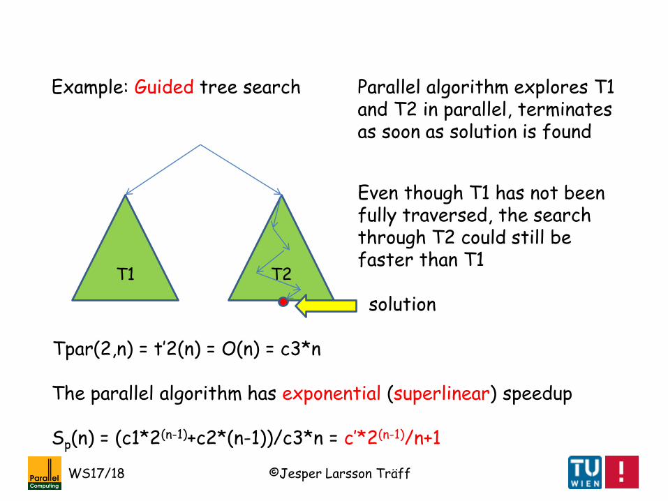
Tseq(n) = T1(n)+t2(n) = O(2(n-1))+O(n-1) = c1*2(n-1) + c2*(n-1)

Sequential algorithm explores all of T1 and one path in T2

Example: Guided tree search

Input size n, solution space/tree of size 2n to be explored

In this algorithm, the fast path in T2 is guided by information gathered when traversing T1


T1 T2

solution

Tpar(2,n) = t’2(n) = O(n) = c3*n

Parallel algorithm explores T1 and T2 in parallel, terminates as soon as solution is found

Example: Guided tree search

The parallel algorithm has exponential (superlinear) speedup

Sp(n) = (c1*2(n-1)+c2*(n-1))/c3*n = c’*2(n-1)/n+1

Even though T1 has not been fully traversed, the search through T2 could still be faster than T1


General case: p subtrees explored in parallel (e.g., master-worker), termination as soon as solution is found in one

Superlinear speedup often found in parallel branch-and-bound search algorithms (solution of hard problems)

Parallel execution exposes better traversal order, not followed by (not “best”) sequential execution: No contradiction to simulation theorem


Sources of superlinear speedup:

a) The memory hierarchyb) Algorithmic reasons (typical case: search trees)c) Non-determinismd) Randomization

a): Different sequential and parallel architecture model

b)-d): Sequential and parallel algorithms are not doing the same things.

A strict, sequential simulation of the parallel algorithm would not exhibit superlinear speedup


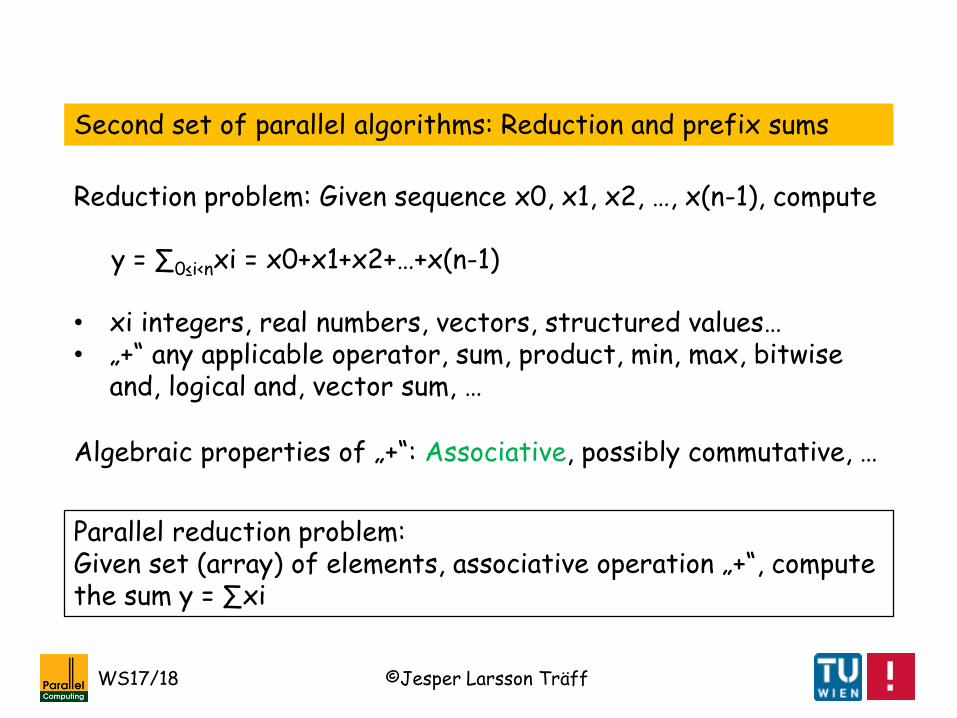
Second set of parallel algorithms: Reduction and prefix sums

Reduction problem: Given sequence x0, x1, x2, …, x(n-1), compute

y = ∑0≤i<nxi = x0+x1+x2+…+x(n-1)

• xi integers, real numbers, vectors, structured values…• „+“ any applicable operator, sum, product, min, max, bitwise

and, logical and, vector sum, …

Algebraic properties of „+“: Associative, possibly commutative, …

Parallel reduction problem:Given set (array) of elements, associative operation „+“, compute the sum y = ∑xi


Collective operation pattern:Set of processors (threads, processes, …) “collectively” invoke some operation, each contribute a subset of the n elements, process order determine element order

• Reduction-to-one: All processors participate in the operations, resulting “sum” stored with one specific processor (“root”)

• Reduction-to-all: All processors participate, results available to all processes

• Reduction-with-scatter: Reduction of vectors, result vector stored in blocks over the processors according to some rule

Reduction is a fundamental, primitive operation, used in many, many applications. Available in some form in most parallel programming models/interfaces as “collective operation”


yi = ∑0≤j<ixj = x0+x1+x2+…+x(i-1)

Definitions:i‘th prefix sum: sum of the first i elements of xi sequence

a) Exclusive prefix (i>0): xi not included in sum (special definitionfor i=0)

yi = ∑0≤j≤ixj = x0+x1+x2+…+xi

b) Inclusive prefix: xi included in sum.Note: Inclusive prefix trivially computable from exclusive prefix(add xi), not vice versa unless „+“ has inverse

Parallel prefix sums problem: Given sequence xi, compute all n prefix sums y0, y1, …, y(n-1)


• Scan: All inclusive prefix sums for process‘s segmentcomputed at process

• Exscan: All exclusive prefix sums for process‘s segmentcomputed at process

Prefix sums fundamental, primitive operation, used for bookkeeping and load balancing purposes (and others) in many, many applications. Available in some form in most parallel programming models/interfaces.

The collective prefix-sums operation often referred to as Scan:

Reduction, Scan:Input sequence x0, x1, x2, …, x(n-1) in array, distributed array, … in form suitable to programming model


Parallel reduction problem:Given set (array) of elements, associative operation „+“, computethe sum y = ∑xi

Parallel prefix-sums problem:Compute all n prefix sums y0, y1, …, y(n-1)

Sequentially, both problems can be solved in O(n) operations, and n-1 applications of “+”.

This is optimal (best possible), since the output depends on each input xi


How to solve prefix sums problem efficiently in parallel?

• Total number of operations (work) proportional to Tseq(n) = O(n)

• Total number of actual „+“ applications close to n-1• Parallel time Tpar(n) = O(n/p+T∞) for large range of p• As fast as possible, T∞(n) = O(log n)

Remark:In most reasonable architecture models, Ω(log n) would be a lower bound on the parallel running time for a work-optimal solution


Sequential solution (both reduction and scan): Simple scanthrough array with running sum

register int sum = x[0];

for (i=1; i<n; i++)

sum += x[i]; x[i] = sum;

Tseq(n) = n-1 summations, O(n), 1 read, 1 write per iteration

for (i=1; i<n; i++)

x[i] = x[i-1]+x[i];

Direct solution, not “best sequential implementation”:2n memory reads

Register solution possibly better, but far from best

Questions: What can the compiler do? How much dependence on basetype (int, long, float, double)? On content?


Some results (the two solutions and the compiler):

Implementation with OpenMP:

traff 60> gcc –o pref –fopenmp <optimization> …

traff 61> gcc --version

gcc (Debian 4.7.2-5) 4.7.2

Copyright (C) 2012 Free Software Foundation, Inc.

This is free software; see the source for copying

conditions. There is NO warranty; not even for

MERCHANTABILITY or FITNESS FOR A PARTICULAR PURPOSE.

Execution on small Intel system

traff 62> more /proc/cpuinfo

…

Model name: Intel (R) Core (TM) i7-2600 CPU @ 3.40 GHz


traff 98> ./pref -n 100000 -t 1

n is 100000 (0 MBytes), threads 1(1)

Basetype 4, block 1 MBytes, block iterations 0

Algorithm Seq straight Time spent 502.37 microseconds

(min 484.67 max 566.68)

Algorithm Seq Time spent 379.09 microseconds (min 296.97

max 397.58)

Algorithm Reduce Time spent 249.39 microseconds (min

210.75 max 309.59)

traff 99> ./pref -n 1000000 -t 1

n is 1000000 (3 MBytes), threads 1(1)

Basetype 4, block 1 MBytes, block iterations 3

Algorithm Seq straight Time spent 3532.19 microseconds

(min 2875.97 max 4552.18)

Algorithm Seq Time spent 2304.72 microseconds (min

2256.46 max 2652.57)

Algorithm Reduce Time spent 1625.14 microseconds (min

1613.68 max 1645.12)


int

No opt -O3

Direct Register Direct Register

100,000 502 379 73 72

1,000,000 3532 2304 615 552

10,000,000 28152 23404 5563 5499

Small custom benchmark, omp_get_wtime() to measure time, 25 repetitions, average running times of prefix-sums function (including function invocation)

Direct, textbook sequential implementation seems slower than register, running-sum implementation. Optimizer can do a lot!

Time in microseconds


double

No opt -O3

Direct Register Direct Register

100,000 451 653 145 144

1,000,000 3926 4454 1466 1162

10,000,000 30411 44344 10231 10001

Surprisingly (?), non-optimized, direct solution faster than register running sum. Optimization a must: Look into other optimization possibilities (flags)

Time in microseconds

Lessons:For “Best sequential implementation”, explore what compiler can do (a lot). Document used compiler options (reproducibility)


Reduction application: Cutoff computation

// Parallelizable partdo

for (i=0; i<n; i++) x[i] = f(i);

// check for convergencedone = …;

while (!done)

done: if x[i]<ε for all i

Each process locally computes

localdone = (x[i]<ε) for all local i

done = allreduce(localdone,AND);

Collective operation: perform reduction overset of involvedprocesses, distributeresult to all processesLocal input

Associative reduction operation


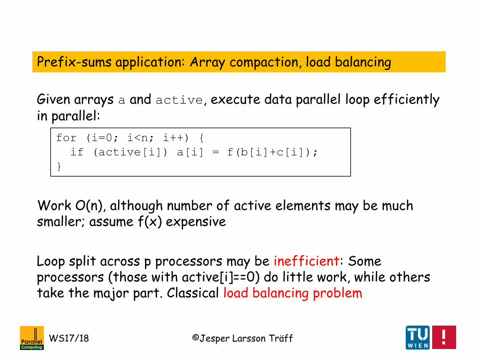
Prefix-sums application: Array compaction, load balancing

for (i=0; i<n; i++)

if (active[i]) a[i] = f(b[i]+c[i]);

Given arrays a and active, execute data parallel loop efficiently in parallel:

Work O(n), although number of active elements may be much smaller; assume f(x) expensive

Loop split across p processors may be inefficient: Some processors (those with active[i]==0) do little work, while others take the major part. Classical load balancing problem


for (i=0; i<n; i++)

if (active[i]) a[i] = f(b[i]+c[i]);

Work O(n), although number of active elements may be muchsmaller; assume f(x) expensive

Solution:Reduce work to O(|active|) by compacting into consecutivepositions of new arrays

Data parallel computation

Given arrays a and active, execute data parallel loop efficientlyin parallel:


a:

Iteration space:for (i=0; i<n; i++) if (active[i]) a[i] = f(b[i]+c[i]);

Dividing into evenly sized blocks inefficient:Work to be balanced is the f(i) computations

Smaller array of active indices:block into evenly sized blocks

…

…


a:


Appoach: Count and index active elements

1. Mark active elements with index 12. Mark non-active element with index 03. Exclusive prefix-sums operation over new index array4. Store original indices in smaller array

…


a:


for (i=0; i<n; i++) index[i] = active[i] ? 1 : 0;

Exscan(index,n); // exclusive prefix computation

m = index[n-1]+(active[n-1) ? 1 : 0);

for (i=0; i<n; i++)

if (active[i]) oldindex[index[i]] = i;

index: 0 0 0 0 0 1 1 1 0 0 0 1 0 0 … 0 0 0 0 0 1 0 … 0 … 1 0 0 … 0 0 1

Exscan 0 0 0 0 0 0 1 2 3 3 3 3 4 4 4 … 4 4 4 4 4 4 5 5 … 5 … 5 6 6

…


a:


for (j=0; j<m; j++)

i = oldindex[j];

a[i] = f(b[i]+c[i]);

1. First load balance (prefix-sums)

2. Then execute (data parallel computation)

…

for (i=0; i<n; i++) index[i] = active[i] ? 1 : 0;


m = index[n-1]+(active[n-1) ? 1 : 0);

for (i=0; i<n; i++)

if (active[i]) oldindex[index[i]] = i;


Prefix-sums application: Partitioning for Quicksort

Quicksort(a,n):1. Select pivot a[k]2. Partition a into a[0,…,n1-1], a[n1,…,n2-1], a[n2,…,n-1] of

elements smaller, equal, and larger than pivot3. In parallel: Quicksort(a,n1), Quicksort(a+n2,n-n2)

Task parallel Quicksort algorithm

Running time (assuming good choice of pivot, at most n/2 elements in either segment):

T(n) ≤ T(n/2)+O(n) with solution T(n) = O(n)

Maximum speedup over sequential O(n log n) Quicksort is therefore O(log n). Need to parallelize partition step


Partition:1. Mark elements smaller than a[k], compact into a[0,…,n1-1]2. Mark elements equal to a[k], compact into a[n1,…,n2-1]3. Mark elements greater than a[k], compact into a[n2,…,n-1]

for (i=0; <n; i++) index[i] = (a[i]<a[k]) ? 1 : 0;


n1 = index[n-1]+(active[n-1] ? 1 : 0);

for (i=0; i<n; i++)

if (a[i]<a[k]) aa[index[i]] = a[i];

// same for equal to and larger than pivot elements

…

// copy back

for (i=0; i<n; i++) a[i] = aa[i];

Another load balancing problem: Assign processors proportionally to smaller and larger segments, Quicksort-recurse (Cilk-lecture)


Quicksort(a,n):1. Select pivot a[k]2. Parallel Partition of a into a[0,…,n1-1], a[n1,…,n2-1],

a[n2,…,n-1] of elements smaller, equal, and larger thanpivot

3. In parallel: Quicksort(a,n1), Quicksort(a+n2,n-n2)

Task parallel Quicksort algorithm with parallel partition

T(n) ≤ T(n/2) + O(log n) with solution T(n) = O(log2 n)

Maximum possible speed-up is now O(n/log n)


Prefix-sums application: load balancing for merge algorithm

<B:

Bad segments: rank[i+1]-rank[i]>m/p

Possible solution:1. Compute total size of bad segments (parallel reduction)2. Assign a proportional number of processors to each bad

segment3. Compute array of size O(p), each entry corresponding to a

processor assigned to a bad segment: start index of segment, size of segment, relative index in segment


b0 b1 b2

p Processors corresponding to bad indices

b = ∑bi Prefix-sums compaction, Reduction, bad segment size bi

a0 0 0 0 … 0 a1 0 0 a2 …

Processors allocated to bi

Number of processors for bi is ai ≈ p*bi/b

A0 A0 … A0 A1...A1 A2 …

0 1 … 2 3 4 … 7 8 …

ix0 ix0 … ix1 ix1 ix2…

1. Ai = ∑0≤j<i: aj (exclusive prefix-sums)

2. Running index by prefix-sums (relative index: running ix-A(i-1))

3. Start index by prefix-sums with max-operation

4. Bad segment start and size, prefix-sums

1.

2.

3.

4.

<p

Start, size


Prefix-sums in gnu C++ STL extensions

#include <parallel/numeric>

#include <vector>

#include <functional>

std::vector<double> v;

__gnu_parallel::

__parallel_partial_sum(v.begin(), v.end(),

v.begin(), std::plus<double>());

Fundamental, parallel operations are being added to STL


1. Recursive: fast, work-optimal2. Non-recursive (iterative): fast, work-optimal3. Doubling: fast(er), not work-optimal (but still useful)

Key to solution: Associativity of „+“:

x0+x1+x2+…+x(n-2)+x(n-1) = ((x0+x1)+(x2+…))+…+(x(n-2)+(xn-1))

All three solutions quite different from sequential solution

Three theoretical solutions to the parallel prefix-sums problem

Questions:• How fast can these algorithms really solve the prefix-sums

problem?• How many operations do they require (work)?


Instead of W(n) = O(n), T(n) = O(n)

++ +++ ++

++ +

+

+

+

+

a[0]

a[1] a[5]a[2] a[4]a[3] a[7]a[6]

a[0] a[1] a[5]a[2] a[4]a[3] a[7]a[6]

something tree-likeW(n) = O(n)T∞(n) = O(log n)


Scan(x,n)

if (n==1) return;

for (i=0; i<n/2; i++) y[i] = x[2*i]+x[2*i+1];

Scan(y,n/2);

x[1] = y[0];

for (i=1; i<n/2; i++)

x[2*i] = y[i-1]+x[2*i];

x[2*i+1] = y[i];

if (odd(n)) x[n-1] = y[n/2-1]+x[n-1];

1. Recursive solution: Sum pairwise, recurse on smaller problem

Reduce problem

Solve recursively

Take back


Scan(x,n)

if (n==1) return;

for (i=0; i<n/2; i++) y[i] = x[2*i]+x[2*i+1];

Scan(y,n/2);

x[1] = y[0];

for (i=1; i<n/2; i++)

x[2*i] = y[i-1]+x[2*i];

x[2*i+1] = y[i];

if (odd(n)) x[n-1] = y[n/2-1]+x[n-1];

1. Recursive solution: Parallelization

Data parallel loop

All processors must havecompleted loop before call

Data parallel loop

Implicit or explicit „barrier“

All processors must havecompleted call before loop


Scan

Pair Pair Pair PairPair …

Return

Scan

Pair Pair Pair PairPair …

Fork-join parallelism, parallel recursive calls

Implied Barrier


1. Recursive solution: Complexity and correctness

Scan(x,n)

if (n==1) return;

for (i=0; i<n/2; i++) y[i] = x[2*i]+x[2*i+1];

Scan(y,n/2);

…

O(n) operations, perfectly parallelizable: O(n/p)

Solve same type of problem, now of size n/2

Total number of „+“ operations W(n) satisfies:• W(1) = O(1)• W(n) ≤ n+W(n/2)


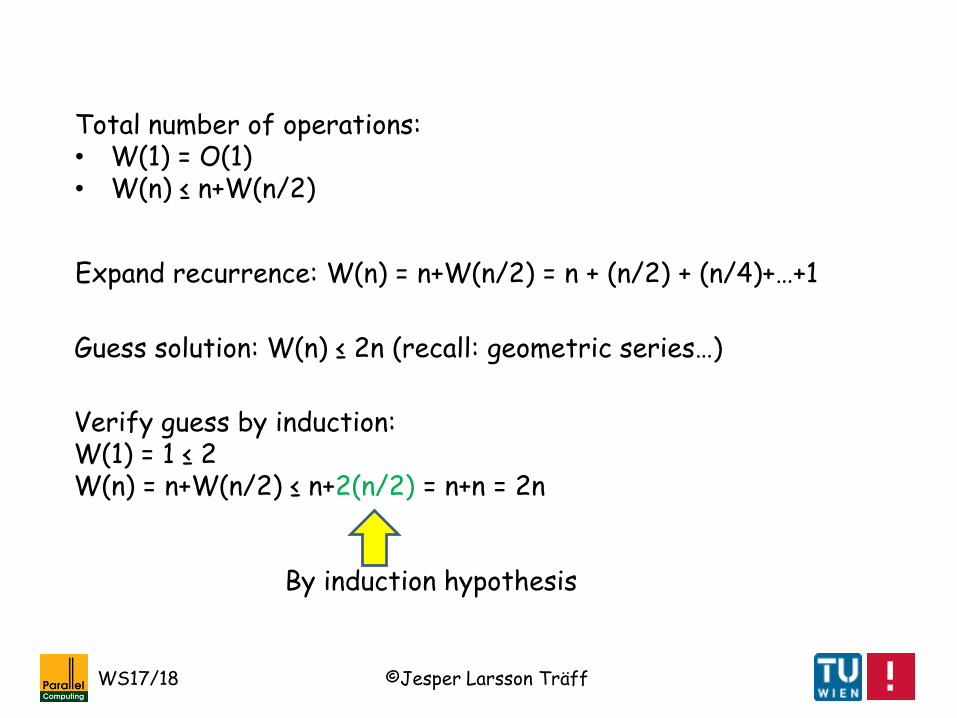
Total number of operations:• W(1) = O(1)• W(n) ≤ n+W(n/2)

Expand recurrence: W(n) = n+W(n/2) = n + (n/2) + (n/4)+…+1

Guess solution: W(n) ≤ 2n (recall: geometric series…)

Verify guess by induction:W(1) = 1 ≤ 2W(n) = n+W(n/2) ≤ n+2(n/2) = n+n = 2n

By induction hypothesis


1. Recursive solution: Complexity and correctness

Scan(x,n)

if (n==1) return;

for (i=0; i<n/2; i++) y[i] = x[2*i]+x[2*i+1];

Scan(y,n/2);

…

O(1) time steps, if n/2 processors available

Solve same problem of size n/2

Number of recursive calls T(n) satisfies• T(1) = O(1)• T(n) ≤ 1+T(n/2)


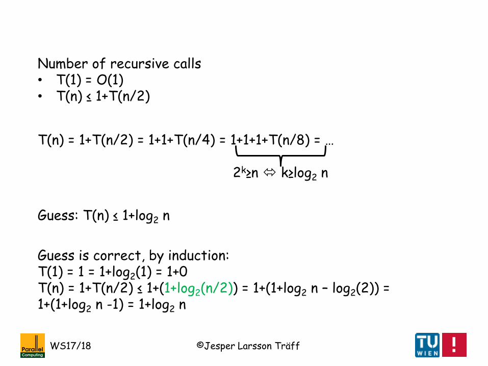
Number of recursive calls• T(1) = O(1)• T(n) ≤ 1+T(n/2)

T(n) = 1+T(n/2) = 1+1+T(n/4) = 1+1+1+T(n/8) = …

2k≥n k≥log2 n

Guess: T(n) ≤ 1+log2 n

Guess is correct, by induction:T(1) = 1 = 1+log2(1) = 1+0T(n) = 1+T(n/2) ≤ 1+(1+log2(n/2)) = 1+(1+log2 n – log2(2)) =1+(1+log2 n -1) = 1+log2 n


Scan(x,n)

if (n==1) return; // base

for (i=0; i<n/2; i++) y[i] = x[2*i]+x[2*i+1];

Scan(y,n/2);

x[1] = y[0];

for (i=1; i<n/2; i++)

x[2*i] = y[i-1]+x[2*i];

x[2*i+1] = y[i];

if (odd(n)) x[n-1] = y[n/2-1]+x[n-1];

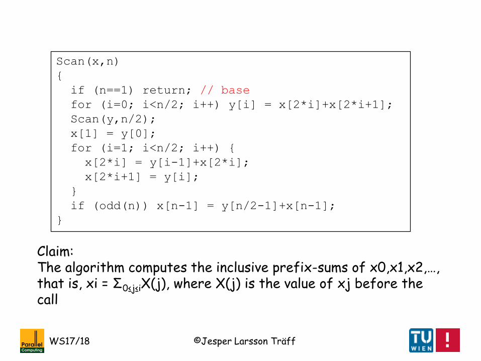
Claim:The algorithm computes the inclusive prefix-sums of x0,x1,x2,…, that is, xi = Σ0≤j≤iX(j), where X(j) is the value of xj before the call


Scan(x,n)


for (i=0; i<n/2; i++) y[i] = x[2*i]+x[2*i+1];

Scan(y,n/2);

x[1] = y[0];

for (i=1; i<n/2; i++)

x[2*i] = y[i-1]+x[2*i];

x[2*i+1] = y[i];

if (odd(n)) x[n-1] = y[n/2-1]+x[n-1];

Proof by induction: Base n=1 is correct, algorithm does nothing


Scan(x,n)


for (i=0; i<n/2; i++) y[i] = x[2*i]+x[2*i+1];

Scan(y,n/2); // by induction hypothesis

x[1] = y[0];

for (i=1; i<n/2; i++)

x[2*i] = y[i-1]+x[2*i];

x[2*i+1] = y[i];

if (odd(n)) x[n-1] = y[n/2-1]+x[n-1];

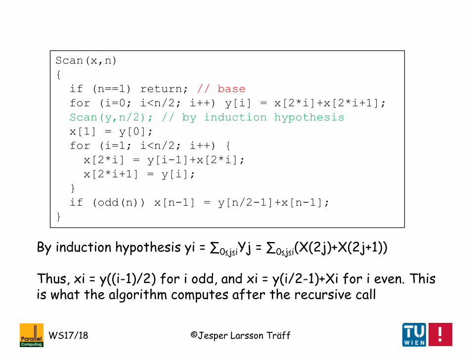
Proof by induction: By induction hypothesis, yi = ∑0≤j≤iYj, where Yj is the value of yjbefore the recursive Scan call, so yi = ∑0≤j≤iYj = ∑0≤j≤i(X(2j)+X(2j+1))


Scan(x,n)


for (i=0; i<n/2; i++) y[i] = x[2*i]+x[2*i+1];

Scan(y,n/2); // by induction hypothesis

x[1] = y[0];

for (i=1; i<n/2; i++)

x[2*i] = y[i-1]+x[2*i];

x[2*i+1] = y[i];

if (odd(n)) x[n-1] = y[n/2-1]+x[n-1];

By induction hypothesis yi = ∑0≤j≤iYj = ∑0≤j≤i(X(2j)+X(2j+1))

Thus, xi = y((i-1)/2) for i odd, and xi = y(i/2-1)+Xi for i even. Thisis what the algorithm computes after the recursive call


1. Recursive solution: Summary

• With enough processors, T∞(n) = 2 log n parallel steps (recursive calls) needed, two barrier synchronizations per recursive call

• Number of operations, W(n) = O(n), all perfectly parallelizable (data parallel)

• Tpar(p,n) = W(n)/p + T∞(n) = O(n/p+log n)

• Linear speed-up up to Tseq(n)/T∞(n) = n/log n processors


1. Recursive solution: Summary (practical considerations)

Drawbacks:• Space: extra n/2 sized array in each recusive call, n in total• About 2n + operations (compared to sequential scan: n-1)• 2(log2n) parallel steps

Advantages:• Smaller y array may fit in cache, pair-wise summing has good

spatial locality (see later)


2. Non-recursive solution: Eliminate recursion and extra space

0 1 2 3 4 5 6 7 8 9 10 11 12 13 14 15 16

x:

round 0

round 3round 2round 1

And almost done, now x[2k-1] = ∑0≤i<2k xi

Perform log2n rounds, in round i, i≥0, a “+” operation is done for every 2i+1’th element

A synchronization operation (barrier) is needed after each round


Lemma:Reduction can be performed out in r = log2 n synchronizedrounds, for n a power of 2. Total number of + operations aren/2+n/4+n/8+…<n (=n-1)

• Shared memory (programming) model: synchronization after each round

• Distributed memory programming model: representcommunication

Recall, geometric series: ∑0≤i≤nari = a(1-rn+1)/1-r)


0 1 2 3 4 5 6 7 8 9 10 11 12 13 14 15 16

x:

round 0


for (k=1; k<n; k=kk)

kk = k<<1; // double

for (i=kk-1; i<n, i+=kk)

x[i] = x[i-k]+x[i];

barrier;

Data parallel computation, n/2(k+1)

operations for round r, r=0, 1, …

Explicit synchronization


0 1 2 3 4 5 6 7 8 9 10 11 12 13 14 15 16

x:

round 0





x[i] = x[i-k]+x[i];

barrier;

Beware ofdependencies




0 1 2 3 4 5 6 7 8 9 10 11 12 13 14 15 16

x:

round 0





x[i] = x[i-k]+x[i];

barrier;

But here are none. Why?

k is kk/2, so noupdate to x[i-k]




x:

Distributed memory programming model

0 1 2 3 4 5 6 7 8 14 15 16…

Prefix-sums problem solved with explicit communication: Message passing programming model

Beware: Too costly for large n relative to p


15

0

Communication pattern: Binomial tree


15

round 0

round 3

round 2

round 1



15

round 0

round 3

round 2

round 1

Property 1:Root active in all rounds



15

Property 2:For l-level tree, number ofnodes at level k, 0≤k<l ischoose(k,l-1), the binomialcoefficient



So far, algorithm can compute the sum for arrays with n=2k

elements for k≥0

• Repair for n not a power of 2?• Extend to parallel prefix-sums?

Observation/invariant: let X be original content of array xBefore round k, k=0,…,floor(log2n)

x[i] = X[i-2k-1]+…+X[i]

for i=j*2k-1, j=1, 2, 3, …

Idea:Prefix sums computed for certain elements, use anther log2n rounds to extend partial prefix sums


Proof by invariant




x[i] = x[i-k]+x[i];

barrier;

Invariant true before0‘th iteration

If I true before k‘thiteration, must be true

before (k+1)‘th

Invariant must implyconclusion/intended result

Home-work: provecorrectness of thisalgorithm


Invariant: X be original content of x. Before round k, k=0,…,floor(log2n), it holds that

x[i] = ∑i-2k+1≤j‘≤iX[j‘] for i=j*2k-1




x[i] = x[i-k]+x[i];

barrier;

Before round k=0, x[i] = ∑i-2k+1≤j‘≤iX[j‘] = ∑i≤j‘≤iX[j‘] = X[i]

True by definition, invariant holds before iterations start

Homework solution

In program, k doubles, round number is log(k); not to confuse with k in invariant


Invariant: X be original content of x. Before round k, k=0,…,floor(log2n), it holds that

x[i] = ∑i-2k+1≤j‘≤iX[j‘] for i=j*2k-1




x[i] = x[i-k]+x[i];

barrier;

In round k, x[i] is updated by x[i-2k]+x[i]. By the invariant this is(∑i-2

k-2

k+1≤j‘≤i-2

kX[j‘]) + (∑i-2k+1≤j‘≤iX[j‘]) = (∑i-2

k-2

k+1≤j‘≤iX[j‘]) = ∑i-

2(k+1)

+1≤j‘≤iX[j‘]. The invariant therefore holds before the k+1‘st iteration

In program, k doubles, round is log(k); not to confuse with k in invariant


0 1 2 3 4 5 6 7 8 9 10 11 12 13 14 15 16

x:

round 0


“Good indices: have correct ∑0≤j≤ix[i]

Extend to prefix-sums

Idea: Use another log n rounds to make remaining indices “good”


0 1 2 3 4 5 6 7 8 9 10 11 12 13 14 15 16

x:

round 0


round 0

round 2round 1

Up phase

Down phase

Extending to prefix-sums





x[i] = x[i-k]+x[i];

barrier;

for (k=k>>1; k>1; k=kk)

kk = k>>1; // halve

for (i=k-1; i<n-kk; i+=k)

x[i+kk] = x[i]+x[i+kk];

barrier;

„up-phase“: log2 n rounds, n/2+n/4+n/8+… < n summations

„down phase“:log2 n rounds, n/2+n/4+n/8+… < n summations

Total work ≈ 2n = O(Tseq(n))

But: factor 2 off from sequential n-1 work

Non-recursive, data parallel implementation

These could be data dependencies, but are not


for (k=k>>1; k>1; k=kk)

kk = k>>1; // halve

for (i=k-1; i<n-kk; i+=k)

x[i+kk] = x[i]+x[i+kk];

barrier;

Correctness: Need to prove that down-phase makes all indices good.

Prove invariant: x[i] = ∑0≤j≤iX[i], for i=j*2k-1, j=1,2,3,…, k=floor(log n), floor(log2n)-1, …

Check at home


0 1 2 3 4 5 6 7 8 9 10 11 12 13 14 15 16

x:

round 0


round 0

round 2round 1

phase 0

phase 1

Sp(n) at most p/2: Half the processors are „lost“


0 1 2 3 4 5 6 7 8 9 10 11 12 13 14 15 16

x:

round 0


round 0

round 2round 1

phase 0

phase 1

For p=n: Work optimal, but not cost optimal. The p processorsare occupied in 2log p rounds = O(p log p)


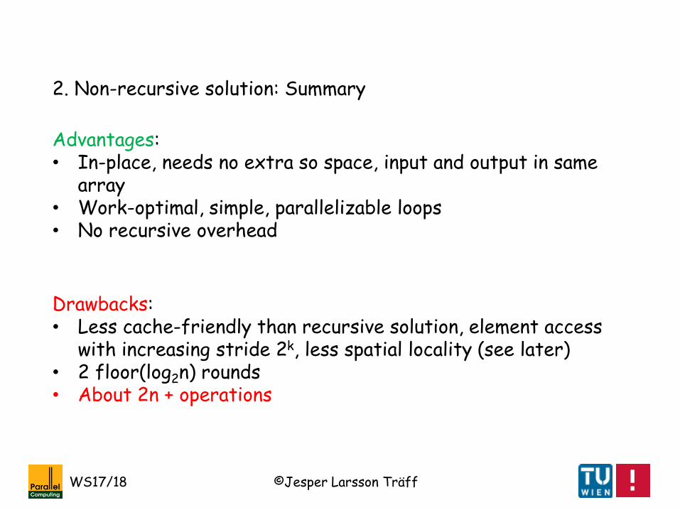
2. Non-recursive solution: Summary

Advantages:• In-place, needs no extra so space, input and output in same

array• Work-optimal, simple, parallelizable loops• No recursive overhead

Drawbacks:• Less cache-friendly than recursive solution, element access

with increasing stride 2k, less spatial locality (see later)• 2 floor(log2n) rounds• About 2n + operations


Aside: A lower bound/tradeoff for prefix-sums

Marc Snir: Depth-Size Trade-Offs for Parallel Prefix Computation. J. Algorithms 7(2): 185-201 (1986)Haikun Zhu, Chung-Kuan Cheng, Ronald L. Graham: On theconstruction of zero-deficiency parallel prefix circuits withminimum depth. ACM Trans. Design Autom. Electr. Syst. 11(2): 387-409 (2006)

Theorem (paraphrase): For computing the prefix sums for an n input sequence, the following tradeoff between “size” s (number of + operations) and “depth” t (T∞) holds: s+t≥2n-2

Proof by examining “circuits” (model of parallel computation) that compute prefix sums

Roughly, this means: For fast parallel prefix sums algorithms, speedup (in terms of + operations) is at most p/2


Prefix-sums for distributed memory models

Distributed memory programming model: represents communication

Algorithm takes 2log2n communication rounds, each with n/2k

concurrent communication operations, total of 2n communication operations. Since often n>>p, too expensive

Blocking technique:

Reduce number of communication/synchronization steps by dividing problem into p similar, smaller problems (of size n/p) that can be solved sequentially (in parallel)


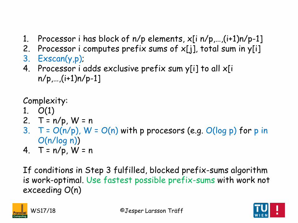
1. Processor i has block of n/p elements, x[i n/p,…,(i+1)n/p-1] 2. Processor i computes prefix sums of x[j], total sum in y[i]3. Exscan(y,p);4. Processor i adds exclusive prefix sum y[i] to all x[i

n/p,…,(i+1)n/p-1]

Observation:Total work (+ operations) is 2n+p log p; at least twice Tseq(n)

Blocking technique for prefix-sums algorithms

Processors locally, without synchronization, computes prefix sums on local (part of) array of size n/p (block). Exscan(exclusive prefix-sums) operation takes O(log p) communication rounds/synchronization steps, and O(p) work. Processors complete by local postprocessing (block).


Prefix-∑ Prefix-∑ Prefix-∑ Prefix-∑x:

y: y[i] = ∑x[j]

Exscan(y,z) z[i] = y[0]+…+y[i-1]

Add z[i] Add z[i] Add z[i]



y: y[i] = ∑x[j]



After solving local problems on block: p elements, p processors.Algorithm that is as fast as possible (small number of rounds) needed, does not need to be work optimal!

Note: This is not the best possible application of the blocking technique (hint: Better to divide into p+1 parts)



y: y[i] = ∑x[i][j]



Sequential computation per processor


∑ ∑ ∑ ∑x:

y: y[i] = ∑x[i][j]


+ Prefix- ∑ + Prefix- ∑ + Prefix- ∑

Observation: Possibly better by reduction first, then prefix-sums

Naïve (per block) analysis:• Prefix first: 2n read, 2n write operations (per block)• Reduction first: 2n read operations, n write operations• Both: ≥2n-1 “+” operations

Why?


Blocking technique summary

Technique:1. Divide problem into p roughly equal sized parts

(subproblems)2. Assign subproblem to each processor3. Solve subproblems using sequential algorithm4. Use parallel algorithm to combine subproblem results5. Apply combined result to subproblem solutions

Analysis:1-2: Should be fast, O(1), O(log n), …3: perfectly parallelizable, e.g. O(n/p)4: Should be fast, e.g. O(log p), total cost must be less than O(n/p)5: Perfectly parallelizable


Blocking technique summary

Technique:1. Divide problem into p roughly equal sized parts

(subproblems)2. Assign subproblem to each processor3. Solve subproblems using sequential algorithm4. Use parallel algorithm to combine subproblem results5. Apply combined result to subproblem solutions

Use when applicable BUT blocking is not always applicable!

Examples:•Prefix-sums – data independent•Cost-optimal merge – data dependent Step 1 quite non-trivial


Blocking technique: Another view

Technique:1. Use work-optimal algorithm to shrink problem enough2. Use fast, possibly non-workoptimal algorithm on shrunk

problem3. Unshrink, compute final solution with work-optimal algorithm

Remark:1. Typically from O(n) to O(n/log n) using O(n/log n) processors2. Use O(n/log n) processors on O(n/log n) sized problem in

O(log n) time steps


Complexity:1. O(1)2. T = n/p, W = n3. T = O(n/p), W = O(n) with p procesors (e.g. O(log p) for p in

O(n/log n))4. T = n/p, W = n

If conditions in Step 3 fulfilled, blocked prefix-sums algorithm is work-optimal. Use fastest possible prefix-sums with work notexceeding O(n)

1. Processor i has block of n/p elements, x[i n/p,…,(i+1)n/p-1] 2. Processor i computes prefix sums of x[j], total sum in y[i]3. Exscan(y,p);4. Processor i adds exclusive prefix sum y[i] to all x[i

n/p,…,(i+1)n/p-1]


3. Yet another data parallel prefix-sums algorithm: Doubling

0 1 32 4 5 76 8

Round k‘, k=2k‘

Idea: In each round, let each processor compute sum x[i] = x[i-k]+x[i] (not only every k’th processor, as in solution 2)

Only ceil(log2n) rounds needed, almost all processors active in each round; correctness by similar argument as solution 2

W. Daniel Hillis, Guy L. Steele Jr.: Data Parallel Algorithms. Commun. ACM 29(12): 1170-1183 (1986)


for (k=1; k<n; k<<=1)

for (i=k; i<n; i++) x[i] = x[i-k]+x[i];

barrier;

3. Yet another data parallel prefix-sums algorithm: doubling

Data parallel?

Why might it not be correct? There are dependencies

• How could this implementation be correct? Why? Invariant?

• All indices i≥1 active in each rounds, total work O(n log n)• But only log n rounds


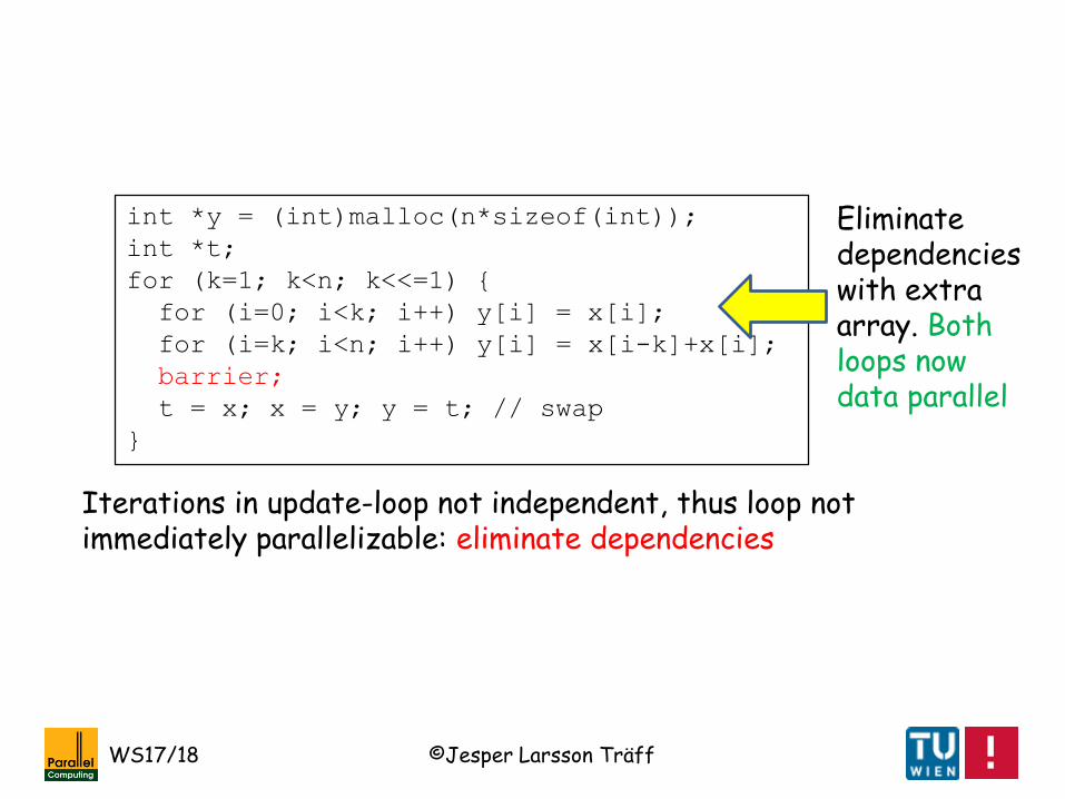
int *y = (int)malloc(n*sizeof(int));

int *t;

for (k=1; k<n; k<<=1)

for (i=0; i<k; i++) y[i] = x[i];

for (i=k; i<n; i++) y[i] = x[i-k]+x[i];

barrier;

t = x; x = y; y = t; // swap

Iterations in update-loop not independent, thus loop not immediately parallelizable: eliminate dependencies

Eliminatedependencieswith extra array. Bothloops nowdata parallel


int *y = (int)malloc(n*sizeof(int));

int *t;

for (k=1; k<n; k<<=1)

for (i=0; i<k; i++) y[i] = x[i];

for (i=k; i<n; i++) y[i] = x[i-k]+x[i];

barrier;

t = x; x = y; y = t; // swap

invariant

Invariant:before iteration step k‘, x[i] = ∑max(0,j-2

k‘+1)≤j≤ix‘[j] for all i

It follows that the algorithm solves the inclusive prefix-sums problem


3. Doubling prefix-sums algorithm: Summary

Advantages:• Only ceil(log2p) rounds (synchronization/communication steps)• Simple, parallelizable loops• No recursive overhead

Drawbacks:• NOT work-optimal• Less cache-friendly than recursive solution, element access

with increasing stride k, less spatial locality (see later)• Extra array of size n needed to eliminate dependencies


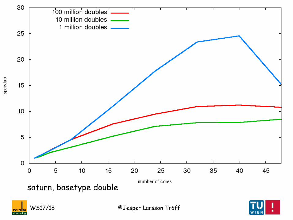
Some results:

We implemented prefix-sums algorithms (with some extra optimizations, and not exactly as just described), and executed on

• saturn: 48-core AMD system, 4*2*6 NUMA-cores, 3-level cache

• mars: 80-core Intel system, 8*10 NUMA-cores, 3-level cache

and computed speedup relative to a good (but probably not “best known/possible”) sequential implementation (25 repetitions of measurement)


mars, basetype double


mars, basetype int


saturn, basetype int


saturn, basetype double


A generalization of the prefix-sums problem: List-ranking

Given list x0 -> x1 -> x2 -> … -> x(n-1), compute all n list-prefix sums

yi = xi+x(i+1)+x(i+2)+…+x(n-1)

by following -> from xi to end of list, “+” some associative operation on type of list elements

Sequentially, looks like an easy problem (similar to prefix sums problem): Follow the pointers and sum up, O(n)

Sometimes called “data-dependent prefix sums problem”


Standard assumption: List stored in array

x0

Head: first element

Tail: last element

x3 x2 x1 x5xn’ x4x6… … …

• Input compactly in array, index of first element may or may not be known

• Index of element in array has no relation to position in list

x:



x0

Head: first element

Tail: last element

x3 x2 x1 x5xn’ x4x6… … …

A difficult problem for parallel computing: What are the subproblems that can be solved independently?

Major, theoretical result (PRAM model): The list ranking problem can be solved in O(n/p+log n) parallel time steps.

Parallel list ranking in practice can work for very large n

x:



x0

Head: first element

Tail: last element

x3 x2 x1 x5xn’ x4x6… … …

Richard J. Anderson, Gary L. Miller: Deterministic Parallel List Ranking. Algorithmica 6(6): 859-868 (1991)

x:

Major, theoretical result (PRAM model): The list ranking problem can be solved in O(n/p+log n) parallel time steps.


Usefulness of list ranking: Tree computations

Example (sketch): Finding levels in rooted tree, tree given as array of parent pointers

Level 0

Level 3

Level 2

Level 1

Level 4

Level 5

Task: Assign each node in tree a level, which is the length of the unique path to the root


Usefulness of list ranking: Tree computations

Make a list that traverses the tree (often possible: Euler tour), assign labels to list pointers, and rank

Label: +1 Label: -1

Level 2

Level 1

Level 3


Technique for problem partitioning: Blocking

Linear time problem with input in n-element array, p processors. Divide array into p independent, consecutive blocks of size Θ(n/p) using O(f(p,n)) time steps per processor. Solve p subproblems in parallel, combine into final solution usingO(g(p,n)) time steps per processor

The resulting parallel algorithm is cost-optimal if both f(p,n) andg(p,n) are O(n/p)

Examples:• Prefix-sums, partition in O(1) time• Merging, partition in O(log n) time

List-ranking problem is not easily solvable by blocking


Other problems for parallel algorithmics

Versatile operations with simple, practical, sequential algorithms and implementations; that are (extremely)difficult to parallelize well, in theory and practice:

Graph search, G=(V,E) (un)directed graph with vertex set V, n=|V| and edge set E, m=|E|, some given source vertex v in V:

• Breadth-first search (BFS)• Depth-first search (DFS)• Single-source shortest path (SSSP)• Transitive closure• …

Hard, graph structure dependentReally Hard; perhaps impossible

Lesson: Building blocks from sequential algorithmics are highly useful for parallel computing algorithms; but not always


Other collective operations

• Broadcast: One processor has data, after operation all processors have data

• Scatter: Data of one processor distributed in blocks to other processors

• Gather: Blocks from all processors collected at one processor• Allgather: Blocks from all processors collected at all

processors (aka Broadcast-to-all)• Alltoall: Each processor has blocks of data, one block for each

other processor, each processor collects blocks from other processor

A set of processors collectively carry out an operation in cooperation on sets of data:


Lecture summary, checklist

• Parallel computing in HPC• FLOPS based efficiency measures (Roofline)• Top500, HPLINPACK

• Moore’s “Law”

• Superlinear speedup

• Prefix sums problem, 4 algorithms• Blocking technique• Prefix sums for load balancing and processor allocation

• List ranking, BFS, DFS, SSSP: Difficult to parallelize problems

Introduction to Parallel Computing - par.tuwien.ac.at · WS17/18 ©Jesper Larsson Träff...

Documents

Transcript of Introduction to Parallel Computing - par.tuwien.ac.at · WS17/18 ©Jesper Larsson Träff...