High-Dimensional Nonlinear Data Assimilation with the Nonlinear ...
3/6/2013 Meto 630; V.Krasnopolsky, "Nonlinear Statistics and NNs" 1
Introduction to Nonlinear Statistics and Neural Networks
Vladimir Krasnopolsky NCEP/NOAA & ESSIC/UMD
http://polar.ncep.noaa.gov/mmab/people/kvladimir.html
3/6/2013 Meto 630; V.Krasnopolsky, "Nonlinear Statistics and NNs" 2
Outline
• Introduction: Regression Analysis • Regression Models (Linear & Nonlinear) • NN Tutorial • Some Atmospheric & Oceanic Applications
– Accurate and fast emulations of model physics – NN Multi-Model Ensemble
• How to Apply NNs • Conclusions

3/6/2013 Meto 630; V.Krasnopolsky, "Nonlinear Statistics and NNs" 3
Evolution in Statistics
• Problems for Classical Paradigm: – Nonlinearity & Complexity – High Dimensionality -
Curse of Dimensionality
• New Paradigm under Construction: – Is still quite fragmentary – Has many different names and
gurus – NNs are one of the tools
developed inside this paradigm
T (years) 1900 – 1949 1950 – 1999 2000 – …
Simple, linear or quasi-linear, single disciplinary, low-dimensional systems
Complex, nonlinear, multi-disciplinary, high-dimensional systems
Simple, linear or quasi-linear, low-dimensional framework of classical
statistics (Fischer, about 1930) Complex, nonlinear, high-dimensional
framework… (NNs) Under Construction!
Objects Studied:
Tools Used:
Teach at the University!

3/6/2013 Meto 630; V.Krasnopolsky, "Nonlinear Statistics and NNs" 4
Problem: Information exists in the form of finite sets of values of
several related variables (sample or training set) – a part of the population:
= {(x1, x2, ..., xn)p, zp}p=1,2,...,N
– x1, x2, ..., xn - independent variables (accurate), – z - response variable (may contain observation
errors ε) We want to find responses z’q for another set of
independent variables = {(x’1, x’2, ..., x’n)q}q=1,..,M
Statistical Inference: A Generic Problem
ℵ′
ℵ
ℵ∉ℵ′

3/6/2013 Meto 630; V.Krasnopolsky, "Nonlinear Statistics and NNs" 5
Regression Analysis (1): General Solution and Its Limitations
Find mathematical function f which describes this relationship: 1. Identify the unknown function f 2. Imitate or emulate the unknown function f
DATA: Training Set {(x1, x2, ..., xn)p, zp}p=1,2,...,N
DATA: Another Set (x’1, x’2, ..., x’n)q=1,2,...,M
zq = f(Xq)
REGRESSION FUNCTION
z = f(X), for all X INDUCTION
Ill-posed problem DEDUCTION Well-posed problem
TRANSDUCTION SVM
Sir Ronald A. Fisher ~ 1930
3/6/2013 Meto 630; V.Krasnopolsky, "Nonlinear Statistics and NNs" 6
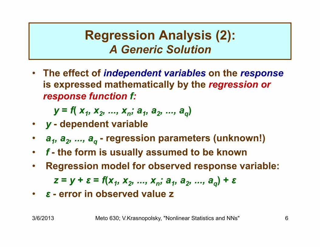
Regression Analysis (2): A Generic Solution
• The effect of independent variables on the response is expressed mathematically by the regression or response function f:
y = f( x1, x2, ..., xn; a1, a2, ..., aq) • y - dependent variable • a1, a2, ..., aq - regression parameters (unknown!) • f - the form is usually assumed to be known • Regression model for observed response variable: z = y + ε = f(x1, x2, ..., xn; a1, a2, ..., aq) + ε • ε - error in observed value z
3/6/2013 Meto 630; V.Krasnopolsky, "Nonlinear Statistics and NNs" 7
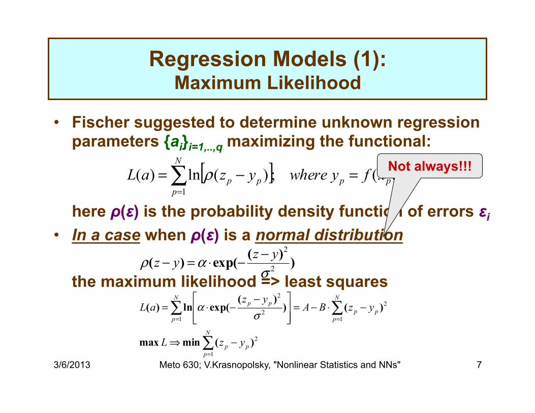
Regression Models (1): Maximum Likelihood
• Fischer suggested to determine unknown regression parameters {ai}i=1,..,q maximizing the functional:
here ρ(ε) is the probability density function of errors εi
• In a case when ρ(ε) is a normal distribution
the maximum likelihood => least squares ))(exp()( 2
2
σαρ yzyz −−⋅=−
[ ] ),(;)(ln)(1
axfywhereyzaL pp
N
ppp =−=∑
=
ρ Not always!!!
∑
∑∑
=
==
−⇒
−⋅−=⎥⎥⎦
⎤
⎢⎢⎣
⎡ −−⋅=
N
ppp
N
ppp
N
p
pp
yzL
yzBAyz
aL
1
2
1
2
12
2
)(minmax
)())(
exp(ln)(σ
α

3/6/2013 Meto 630; V.Krasnopolsky, "Nonlinear Statistics and NNs" 8
Regression Models (2): Method of Least Squares
• To find unknown regression parameters {ai}i=1,2,...,q , the method of least squares can be applied:
• E(a1,...,aq) - error function = the sum of squared
deviations. • To estimate {ai}i=1,2,...,q => minimize E => solve the
system of equations: • Linear and nonlinear cases.
E a a a z y z f x x a a aq p pp
N
p n p qp
N
( , ,..., ) ( ) [ (( ,..., ) ; , ,..., )]1 22
11 1 2
2
1= − = −
= =∑ ∑
∂∂Ea
i qi= =0 12; , ,...,

3/6/2013 Meto 630; V.Krasnopolsky, "Nonlinear Statistics and NNs" 9
Regression Models (3): Examples of Linear Regressions
• Simple Linear Regression: z = a0 + a1 x1 + ε
• Multiple Linear Regression: z = a0 + a1 x1 + a2 x2 + ... + ε =
• Generalized Linear Regression: z = a0 + a1 f1(x1)+ a2 f2(x2) + ... + ε =
– Polynomial regression, fi(x) = xi, z = a0 + a1 x+ a2 x2 + a3 x3 + ... + ε
– Trigonometric regression, fi(x) = cos(ix) z = a0 + a1 cos(x) + a1 cos(2 x) + ... + ε
a a xi ii
n
01
+ +=∑ ε
a a f xi i ii
n
01
+ +=∑ ( ) ε
No free parameters
3/6/2013 Meto 630; V.Krasnopolsky, "Nonlinear Statistics and NNs" 10
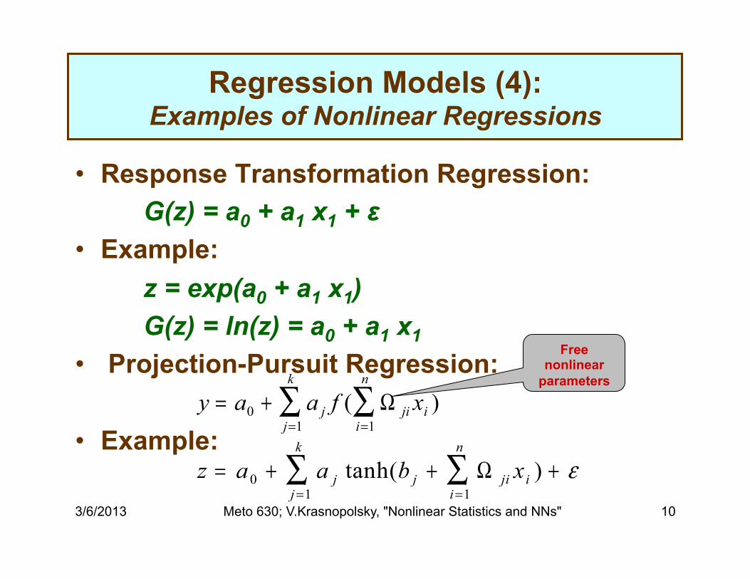
• Response Transformation Regression: G(z) = a0 + a1 x1 + ε
• Example: z = exp(a0 + a1 x1) G(z) = ln(z) = a0 + a1 x1
• Projection-Pursuit Regression: • Example:
Regression Models (4): Examples of Nonlinear Regressions
y a a f xj ji ii
n
j
k
= +==∑∑011
( )Ω
z a a b xj j ji ii
n
j
k
= + + +==∑∑011
tanh( )Ω ε
Free nonlinear
parameters

3/6/2013 Meto 630; V.Krasnopolsky, "Nonlinear Statistics and NNs" 11
NN Tutorial: Introduction to Artificial NNs
• NNs as Continuous Input/Output Mappings – Continuous Mappings: definition and some
examples – NN Building Blocks: neurons, activation
functions, layers – Some Important Theorems
• NN Training • Major Advantages of NNs • Some Problems of Nonlinear Approaches

3/6/2013 Meto 630; V.Krasnopolsky, "Nonlinear Statistics and NNs" 12
• Mapping: A rule of correspondence established between vectors in vector spaces and that associates each vector X of a vector space with a vector Y in another vector space .
Mapping Generalization of Function
mℜnℜ
⎥⎥⎥⎥
⎦
⎤
⎢⎢⎢⎢
⎣
⎡
=
==
≠⎪⎭
⎪⎬
⎫
ℜ∈=
ℜ∈==
),...,,(
),...,,(),...,,(
},,...,,{
},,...,,{)(
nmm
n
n
mm
nn
xxxfy
xxxfyxxxfy
yyyY
xxxXXFY
21
2122
2111
21
21
nℜmℜ
3/6/2013 Meto 630; V.Krasnopolsky, "Nonlinear Statistics and NNs" 13
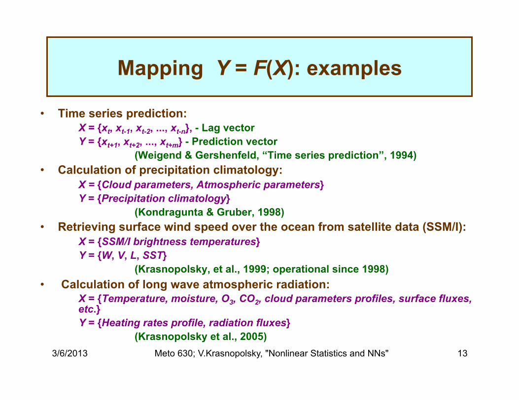
Mapping Y = F(X): examples
• Time series prediction: X = {xt, xt-1, xt-2, ..., xt-n}, - Lag vector
Y = {xt+1, xt+2, ..., xt+m} - Prediction vector (Weigend & Gershenfeld, “Time series prediction”, 1994)
• Calculation of precipitation climatology: X = {Cloud parameters, Atmospheric parameters} Y = {Precipitation climatology}
(Kondragunta & Gruber, 1998) • Retrieving surface wind speed over the ocean from satellite data (SSM/I):
X = {SSM/I brightness temperatures} Y = {W, V, L, SST} (Krasnopolsky, et al., 1999; operational since 1998)
• Calculation of long wave atmospheric radiation: X = {Temperature, moisture, O3, CO2, cloud parameters profiles, surface fluxes, etc.} Y = {Heating rates profile, radiation fluxes} (Krasnopolsky et al., 2005)
3/6/2013 Meto 630; V.Krasnopolsky, "Nonlinear Statistics and NNs" 14
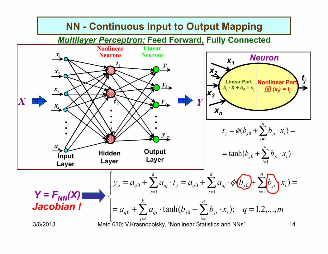
NN - Continuous Input to Output Mapping Multilayer Perceptron: Feed Forward, Fully Connected
1x
2x
3x
4x
nx
1y
2y
3y
my
1t
2t
kt
NonlinearNeurons
LinearNeurons
X Y
Input Layer
Output Layer
Hidden Layer
Y = FNN(X) Jacobian !
x1 x2
x3
xn
tj Linear Part bj · X + b0 = sj
Nonlinear Part (sj) = tj
Neuron
)tanh(
)(
10
10
∑
∑
=
=
⋅+=
=⋅+=
n
iijij
n
iijijj
xbb
xbbt φ
⎪⎪⎩
⎪⎪⎨
⎧
=⋅+⋅+=
=⋅+⋅+=⋅+=
∑ ∑
∑ ∑∑
= =
= ==
mqxbbaa
xbbaataay
k
j
n
iijijqjq
k
j
n
iijijqjq
k
jjqjqq
,...,2,1);tanh(
)(
1 100
1 100
10 φ

3/6/2013 Meto 630; V.Krasnopolsky, "Nonlinear Statistics and NNs" 15
Some Popular Activation Functions tanh(x) Sigmoid, (1 + exp(-x))-1
Hard Limiter Ramp Function
X X
X X

3/6/2013 Meto 630; V.Krasnopolsky, "Nonlinear Statistics and NNs" 16
NN as a Universal Tool for Approximation of Continuous & Almost Continuous Mappings
Some Basic Theorems: " Any function or mapping Z = F (X), continuous on
a compact subset, can be approximately represented by a p (p 3) layer NN in the sense of uniform convergence (e.g., Chen & Chen, 1995; Blum and Li, 1991, Hornik, 1991; Funahashi, 1989, etc.)
" The error bounds for the uniform approximation on compact sets (Attali & Pagès, 1997):
||Z -Y|| = ||F (X) - FNN (X)|| ~ C/k k -number of neurons in the hidden layer C – does not depend on n (avoiding Curse of Dimensionality!)

3/6/2013 Meto 630; V.Krasnopolsky, "Nonlinear Statistics and NNs" 17
NN training (1)
• For the mapping Z = F (X) create a training set - set of matchups {Xi, Zi}i=1,...,N, where Xi is input vector and Zi - desired output vector
• Introduce an error or cost function E:
E(a,b) = ||Z - Y|| = ,
where Y = FNN(X) is neural network
• Minimize the cost function: min{E(a,b)} and find optimal weights (a0, b0)
• Notation: W = {a, b} - all weights.
2
1)(∑
=
−N
iiNNi XFZ

3/6/2013 Meto 630; V.Krasnopolsky, "Nonlinear Statistics and NNs" 18
NN Training (2) One Training Iteration
W
E ≤

3/6/2013 Meto 630; V.Krasnopolsky, "Nonlinear Statistics and NNs" 19
Backpropagation (BP) Training Algorithm
• BP is a simplified steepest descent:
where W - any weight, E - error function, η - learning rate, and ΔW - weight increment • Derivative can be calculated analytically:
• Weight adjustment after r-th iteration: Wr+1 = Wr + ΔW • BP training algorithm is robust but slow
E
WW r+1 W r
W
.0>∂∂WE
WEW
∂∂−=Δ η
∑= ∂
∂⋅−−=∂∂ N
i
iNNiNNi W
XFXFZWE
1
)()]([2
3/6/2013 Meto 630; V.Krasnopolsky, "Nonlinear Statistics and NNs" 20
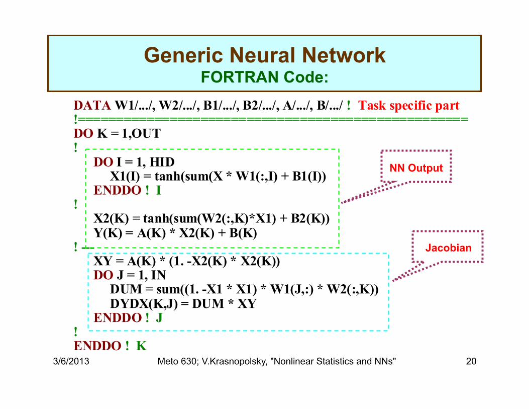
Generic Neural Network FORTRAN Code:
DATA W1/.../, W2/.../, B1/.../, B2/.../, A/.../, B/.../ ! Task specific part!===================================================DO K = 1,OUT! DO I = 1, HID X1(I) = tanh(sum(X * W1(:,I) + B1(I)) ENDDO ! I! X2(K) = tanh(sum(W2(:,K)*X1) + B2(K)) Y(K) = A(K) * X2(K) + B(K) ! --- XY = A(K) * (1. -X2(K) * X2(K)) DO J = 1, IN DUM = sum((1. -X1 * X1) * W1(J,:) * W2(:,K)) DYDX(K,J) = DUM * XY ENDDO ! J ! ENDDO ! K
NN Output
Jacobian

3/6/2013 Meto 630; V.Krasnopolsky, "Nonlinear Statistics and NNs" 21
Major Advantages of NNs :
" NNs are very generic, accurate and convenient mathematical (statistical) models which are able to emulate numerical model components, which are complicated nonlinear input/output relationships (continuous or almost continuous mappings ).
" NNs avoid Curse of Dimensionality " NNs are robust with respect to random noise and fault-
tolerant. " NNs are analytically differentiable (training, error and
sensitivity analyses): almost free Jacobian! " NNs emulations are accurate and fast but NO FREE LUNCH! " Training is complicated and time consuming nonlinear
optimization task; however, training should be done only once for a particular application!
" Possibility of online adjustment " NNs are well-suited for parallel and vector processing

3/6/2013 Meto 630; V.Krasnopolsky, "Nonlinear Statistics and NNs" 22
NNs & Nonlinear Regressions: Limitations (1)
• Flexibility and Interpolation:
• Overfitting, Extrapolation:

3/6/2013 Meto 630; V.Krasnopolsky, "Nonlinear Statistics and NNs" 23
NNs & Nonlinear Regressions: Limitations (2)
• Consistency of estimators: α is a consistent estimator of parameter A, if α → A as the size of the sample n → N, where N is the size of the population.
• For NNs and Nonlinear Regressions consistency can be usually “proven” only numerically.
• Additional independent data sets are required for test (demonstrating consistency of estimates).

3/6/2013 Meto 630; V.Krasnopolsky, "Nonlinear Statistics and NNs" 24
ARTIFICIAL NEURAL NETWORKS: BRIEF HISTORY
• 1943 - McCulloch and Pitts introduced a model of the neuron
• 1962 - Rosenblat introduced the one layer "perceptrons", the model neurons, connected up in a simple fashion.
• 1969 - Minsky and Papert published the book which practically “closed the field”

3/6/2013 Meto 630; V.Krasnopolsky, "Nonlinear Statistics and NNs" 25
ARTIFICIAL NEURAL NETWORKS: BRIEF HISTORY
• 1986 - Rumelhart and McClelland proposed the "multilayer perceptron" (MLP) and showed that it is a perfect application for parallel distributed processing.
• From the end of the 80's there has been explosive growth in applying NNs to various problems in different fields of science and technology

3/6/2013 Meto 630; V.Krasnopolsky, "Nonlinear Statistics and NNs" 26
Atmospheric and Oceanic NN Applications
• Satellite Meteorology and Oceanography – Classification Algorithms – Pattern Recognition, Feature Extraction Algorithms – Change Detection & Feature Tracking Algorithms – Fast Forward Models for Direct Assimilation – Accurate Transfer Functions (Retrieval Algorithms)
• Predictions – Geophysical time series – Regional climate – Time dependent processes
• NN Ensembles – Fast NN ensemble – Multi-model NN ensemble – NN Stochastic Physics
• Fast NN Model Physics • Data Fusion & Data Mining • Interpolation, Extrapolation & Downscaling • Nonlinear Multivariate Statistical Analysis • Hydrological Applications
3/6/2013 Meto 630; V.Krasnopolsky, "Nonlinear Statistics and NNs" 27
Developing Fast NN Emulations for Parameterizations of Model Physics
Atmospheric Long & Short Wave Radiations
3/6/2013 Meto 630; V.Krasnopolsky, "Nonlinear Statistics and NNs" 28
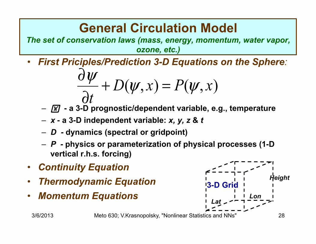
General Circulation Model The set of conservation laws (mass, energy, momentum, water vapor,
ozone, etc.) • First Priciples/Prediction 3-D Equations on the Sphere:
– - a 3-D prognostic/dependent variable, e.g., temperature – x - a 3-D independent variable: x, y, z & t – D - dynamics (spectral or gridpoint) – P - physics or parameterization of physical processes (1-D
vertical r.h.s. forcing)
• Continuity Equation • Thermodynamic Equation • Momentum Equations
( , ) ( , )D x P xtψ ψ ψ∂ + =∂
Lon Lat
Height 3-D Grid
3/6/2013 Meto 630; V.Krasnopolsky, "Nonlinear Statistics and NNs" 29
General Circulation Model Physics – P, represented by 1-D (vertical) parameterizations
• Major components of P = {R, W, C, T, S}: – R - radiation (long & short wave processes) – W – convection, and large scale precipitation processes – C - clouds – T – turbulence – S – surface model (land, ocean, ice – air interaction)
• Each component of P is a 1-D parameterization of complicated set of multi-scale theoretical and empirical physical process models simplified for computational reasons
• P is the most time consuming part of GCMs!

3/6/2013 Meto 630; V.Krasnopolsky, "Nonlinear Statistics and NNs" 30
Distribution of Total Climate Model Calculation Time 12%
66%
22%
DynamicsPhysicsOther
Current NCAR Climate Model (T42 x L26): 3 x 3.5
6%
89%
5%
Near-Term Upcoming Climate Models (estimated) : 1 x
1
3/6/2013 Meto 630; V.Krasnopolsky, "Nonlinear Statistics and NNs" 31
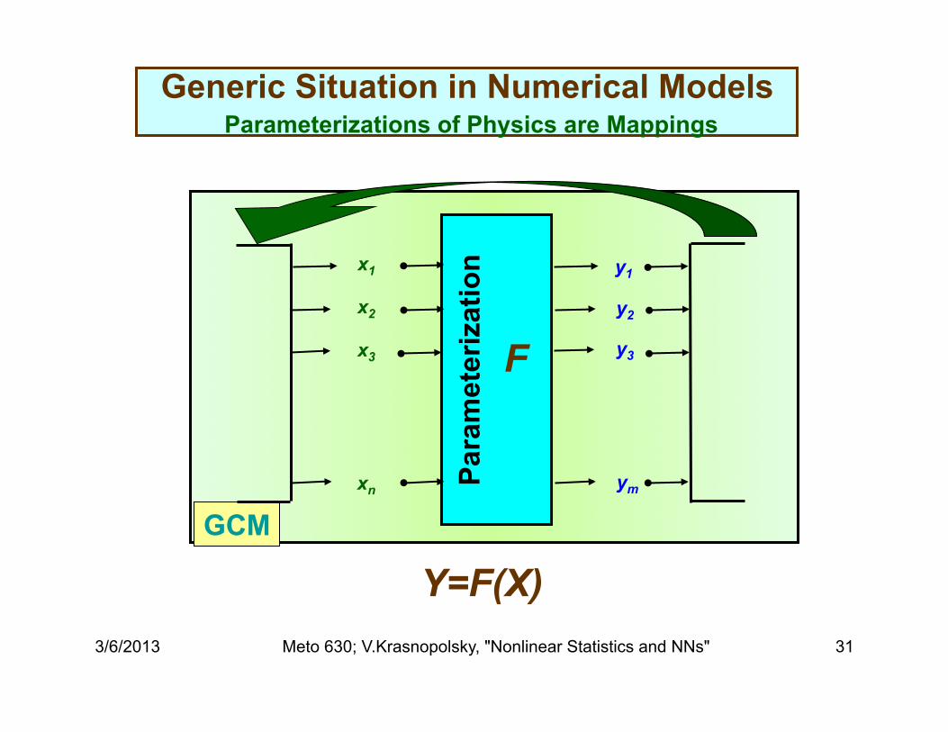
Generic Situation in Numerical Models Parameterizations of Physics are Mappings
GCM
x1
x2
x3
xn
y1
y2
y3
ym Para
met
eriz
atio
n
Y=F(X)
F

3/6/2013 Meto 630; V.Krasnopolsky, "Nonlinear Statistics and NNs" 32
Generic Solution – “NeuroPhysics” Accurate and Fast NN Emulation for Physics Parameterizations
Learning from Data
GCM
X Y
Original Parameterization
F
X Y
NN Emulation
FNN
Training Set …, {Xi, Yi}, … Xi
Dphys
NN Emulation
FNN

3/6/2013 Meto 630; V.Krasnopolsky, "Nonlinear Statistics and NNs" 33
NN for NCAR CAM Physics CAM Long Wave Radiation
• Long Wave Radiative Transfer:
• Absorptivity & Emissivity (optical properties):
4
( ) ( ) ( , ) ( , ) ( )
( ) ( ) ( , ) ( )
( ) ( )
t
s
p
t t tp
p
sp
F p B p p p p p dB p
F p B p p p dB p
B p T p the Stefan Boltzman relation
ε α
α
σ
↓
↑
′= ⋅ + ⋅
′ ′= − ⋅
= ⋅ − −
∫
∫
0
0
{ ( ) / ( )} (1 ( , ))( , )
( ) / ( )
( ) (1 ( , ))( , )
( )( )
t t
tt
dB p dT p p p dp p
dB p dT p
B p p p dp p
B pB p the Plank function
ν ν
ν ν
ν
τ να
τ νε
∞
∞
′ ′ ′⋅ − ⋅′ =
⋅ − ⋅=
−
∫
∫
3/6/2013 Meto 630; V.Krasnopolsky, "Nonlinear Statistics and NNs" 34
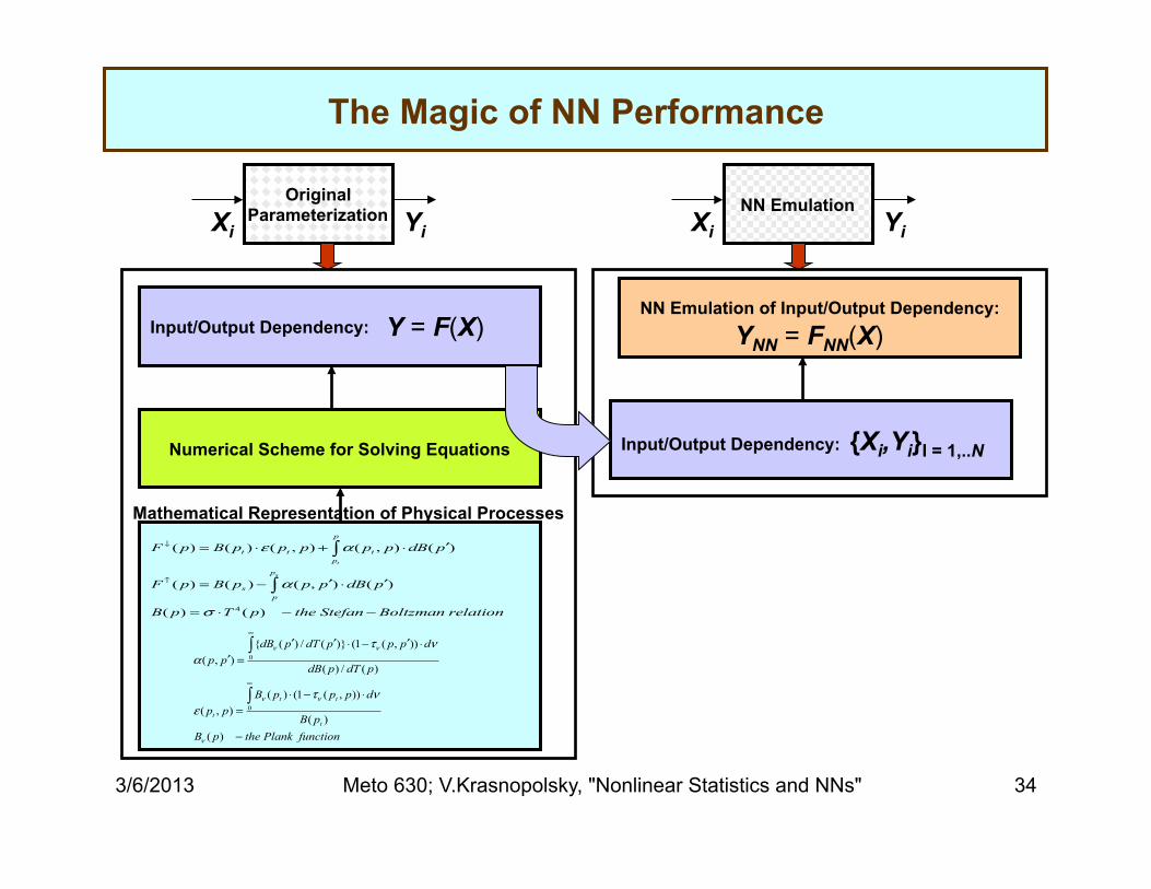
NN Emulation of Input/Output Dependency: Input/Output Dependency:
The Magic of NN Performance
Xi Original
Parameterization Yi
Y = F(X)
Xi NN Emulation
Yi
YNN = FNN(X)
Mathematical Representation of Physical Processes
4
( ) ( ) ( , ) ( , ) ( )
( ) ( ) ( , ) ( )
( ) ( )
t
s
p
t t tp
p
sp
F p B p p p p p dB p
F p B p p p dB p
B p T p the Stefan Boltzman relation
ε α
α
σ
↓
↑
′= ⋅ + ⋅
′ ′= − ⋅
= ⋅ − −
∫
∫
0
0
{ ( ) / ( )} (1 ( , ))( , )
( ) / ( )
( ) (1 ( , ))( , )
( )( )
t t
tt
dB p dT p p p dp p
dB p dT p
B p p p dp p
B pB p the Plank function
ν ν
ν ν
ν
τ να
τ νε
∞
∞
′ ′ ′⋅ − ⋅′ =
⋅ − ⋅=
−
∫
∫
Numerical Scheme for Solving Equations Input/Output Dependency: {Xi,Yi}I = 1,..N

3/6/2013 Meto 630; V.Krasnopolsky, "Nonlinear Statistics and NNs" 35
Neural Networks for NCAR (NCEP) LW Radiation NN characteristics
• 220 (612 for NCEP) Inputs: – 10 Profiles: temperature; humidity; ozone, methane, cfc11, cfc12, & N2O mixing
ratios, pressure, cloudiness, emissivity – Relevant surface characteristics: surface pressure, upward LW flux on a
surface - flwupcgs • 33 (69 for NCEP) Outputs:
– Profile of heating rates (26)
– 7 LW radiation fluxes: flns, flnt, flut, flnsc, flntc, flutc, flwds • Hidden Layer: One layer with 50 to 300 neurons • Training: nonlinear optimization in the space with
dimensionality of 15,000 to 100,000 – Training Data Set: Subset of about 200,000 instantaneous profiles simulated by
CAM for the 1-st year – Training time: about 1 to several days (SGI workstation) – Training iterations: 1,500 to 8,000
• Validation on Independent Data: – Validation Data Set (independent data): about 200,000 instantaneous profiles
simulated by CAM for the 2-nd year

3/6/2013 Meto 630; V.Krasnopolsky, "Nonlinear Statistics and NNs" 36
Neural Networks for NCAR (NCEP) SW Radiation NN characteristics
• 451 (650 NCEP) Inputs: – 21 Profiles: specific humidity, ozone concentration, pressure, cloudiness,
aerosol mass mixing ratios, etc – 7 Relevant surface characteristics
• 33 (73 NCEP) Outputs: – Profile of heating rates (26) – 7 LW radiation fluxes: fsns, fsnt, fsdc, sols, soll, solsd, solld
• Hidden Layer: One layer with 50 to 200 neurons • Training: nonlinear optimization in the space with
dimensionality of 25,000 to 130,000 – Training Data Set: Subset of about 200,000 instantaneous profiles simulated by
CAM for the 1-st year – Training time: about 1 to several days (SGI workstation) – Training iterations: 1,500 to 8,000
• Validation on Independent Data: – Validation Data Set (independent data): about 100,000 instantaneous profiles
simulated by CAM for the 2-nd year
3/6/2013 Meto 630; V.Krasnopolsky, "Nonlinear Statistics and NNs" 37
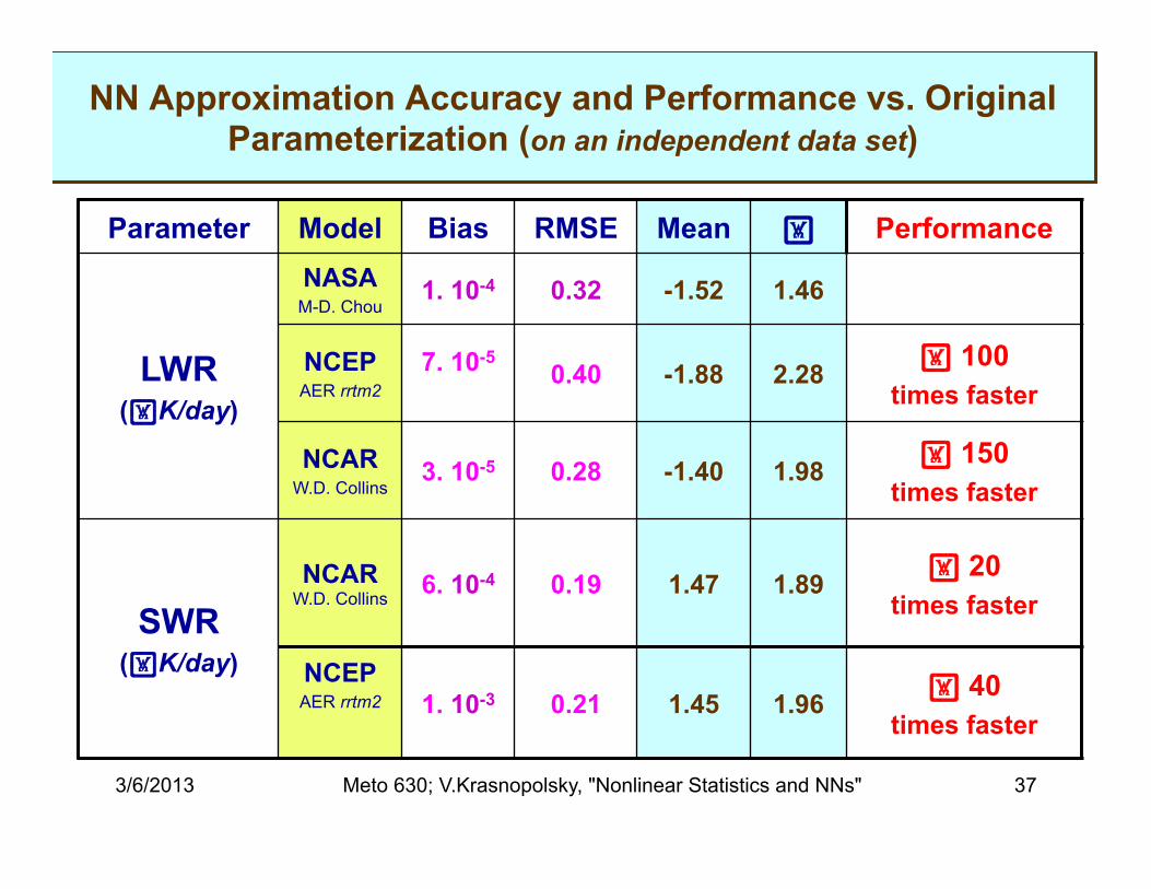
NN Approximation Accuracy and Performance vs. Original Parameterization (on an independent data set)
Parameter Model Bias RMSE Mean Performance
LWR (K/day)
NASA M-D. Chou
1. 10-4 0.32 -1.52 1.46
NCEP AER rrtm2
7. 10-5 0.40 -1.88 2.28 100
times faster
NCAR W.D. Collins
3. 10-5 0.28 -1.40 1.98 150 times faster
SWR (K/day)
NCAR W.D. Collins
6. 10-4 0.19 1.47 1.89 20 times faster
NCEP AER rrtm2
1. 10-3 0.21 1.45 1.96 40
times faster

3/6/2013 Meto 630; V.Krasnopolsky, "Nonlinear Statistics and NNs" 38
Individual Profiles
PRMSE = 0.11 & 0.06 K/day PRMSE = 0.05 & 0.04 K/day
Black – Original Parameterization Red – NN with 100 neurons Blue – NN with 150 neurons
PRMSE = 0.18 & 0.10 K/day

3/6/2013 Meto 630; V.Krasnopolsky, "Nonlinear Statistics and NNs" 39
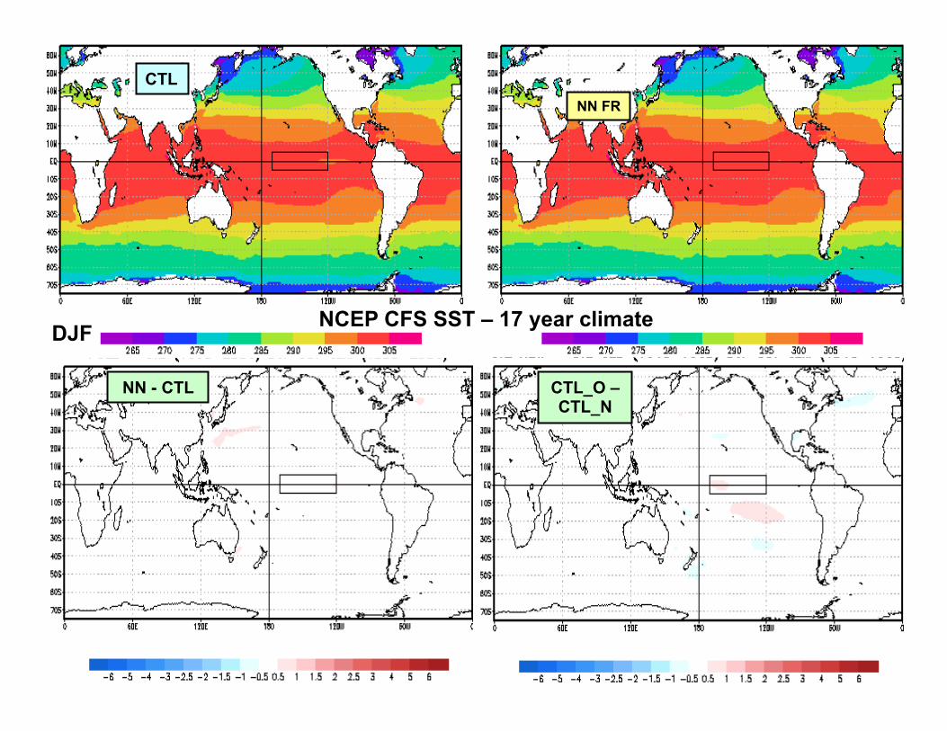
NCAR CAM-2: 50 YEAR EXPERIMENTS NCEP CFS: 17 YEAR EXPERIMENTS
• CONTROL RUN: the standard NCAR CAM or NCEP CFS versions with the original Radiation (LWR and SWR)
• NN RUN: the hybrid version of NCAR CAM or NCEP CFS with NN emulation of the LWR & SWR

3/6/2013 Meto 630; V.Krasnopolsky, "Nonlinear Statistics and NNs" 40
NCAR CAM-2 Zonal Mean U 50 Year Average
(a) – Original LWR Parameterization
(b) - NN Approximation (c) - Difference (a) – (b),
contour 0.2 m/sec
all in m/sec
3/6/2013 Meto 630; V.Krasnopolsky, "Nonlinear Statistics and NNs" 41
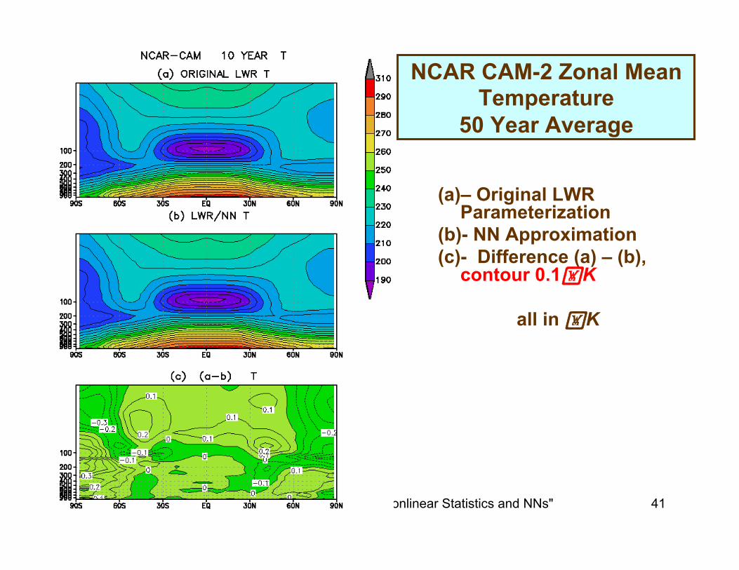
NCAR CAM-2 Zonal Mean Temperature
50 Year Average
(a) – Original LWR Parameterization
(b) - NN Approximation (c) - Difference (a) – (b),
contour 0.1K
all in K
3/6/2013 Meto 630; V.Krasnopolsky, "Nonlinear Statistics and NNs" 42
CTL NN FR
NN - CTL CTL_O – CTL_N
DJF NCEP CFS SST – 17 year climate
3/6/2013 Meto 630; V.Krasnopolsky, "Nonlinear Statistics and NNs" 43
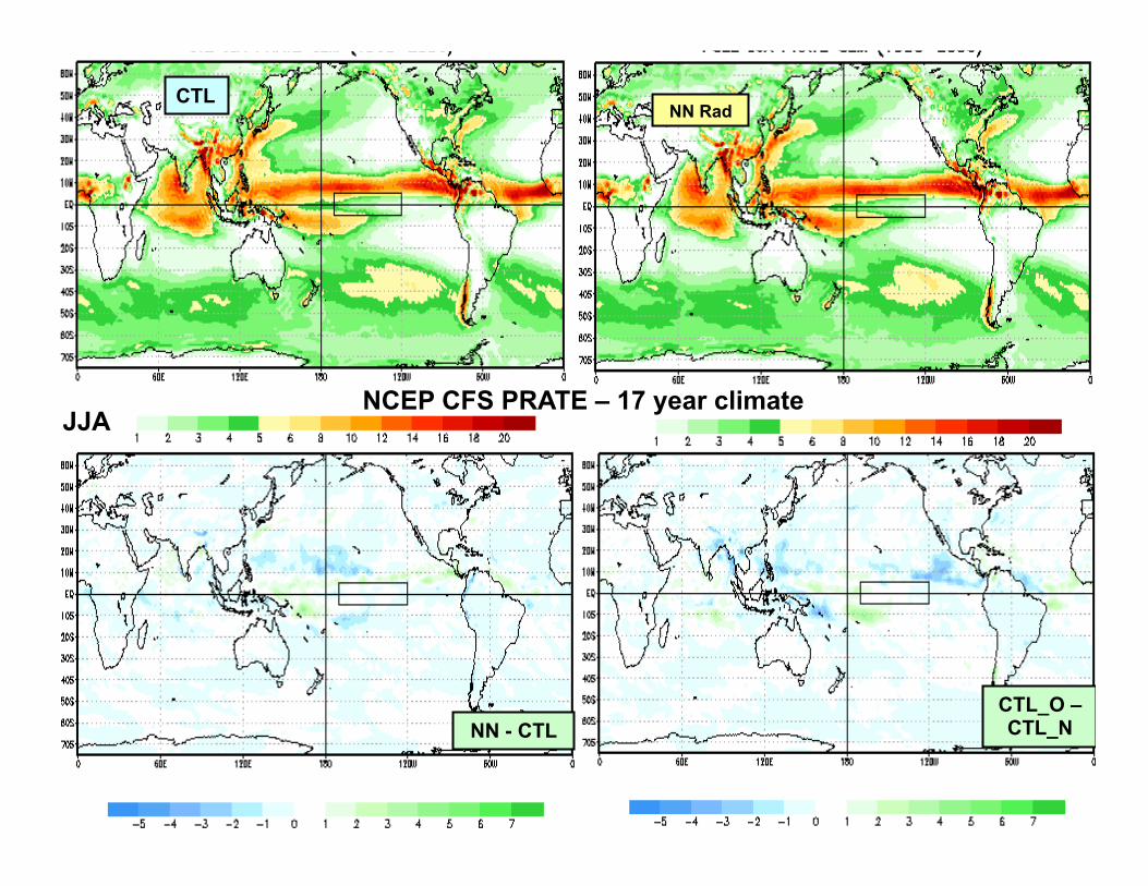
CTL NN Rad
NN - CTL CTL_O – CTL_N
JJA NCEP CFS PRATE – 17 year climate
3/6/2013 Meto 630; V.Krasnopolsky, "Nonlinear Statistics and NNs" 44
Application of the Neural Network Technique to Develop a Nonlinear Multi-Model
Ensemble for Precipitations over ConUS
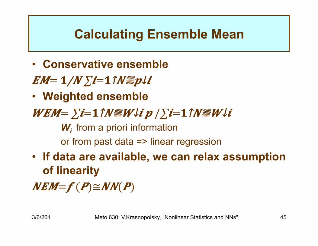
Calculating Ensemble Mean
• Conservative ensemble 𝑬𝑴= 𝟏/𝑵 ∑𝒊=𝟏↑𝑵▒𝒑↓𝒊 • Weighted ensemble 𝑾𝑬𝑴= ∑𝒊=𝟏↑𝑵▒𝑾↓𝒊 𝒑 /∑𝒊=𝟏↑𝑵▒𝑾↓𝒊
Wi from a priori information or from past data => linear regression
• If data are available, we can relax assumption of linearity
𝑵𝑬𝑴=𝒇 (𝑷)≅𝑵𝑵(𝑷)
3/6/201 Meto 630; V.Krasnopolsky, "Nonlinear Statistics and NNs" 45
3/6/2013 Meto 630; V.Krasnopolsky, "Nonlinear Statistics and NNs" 46
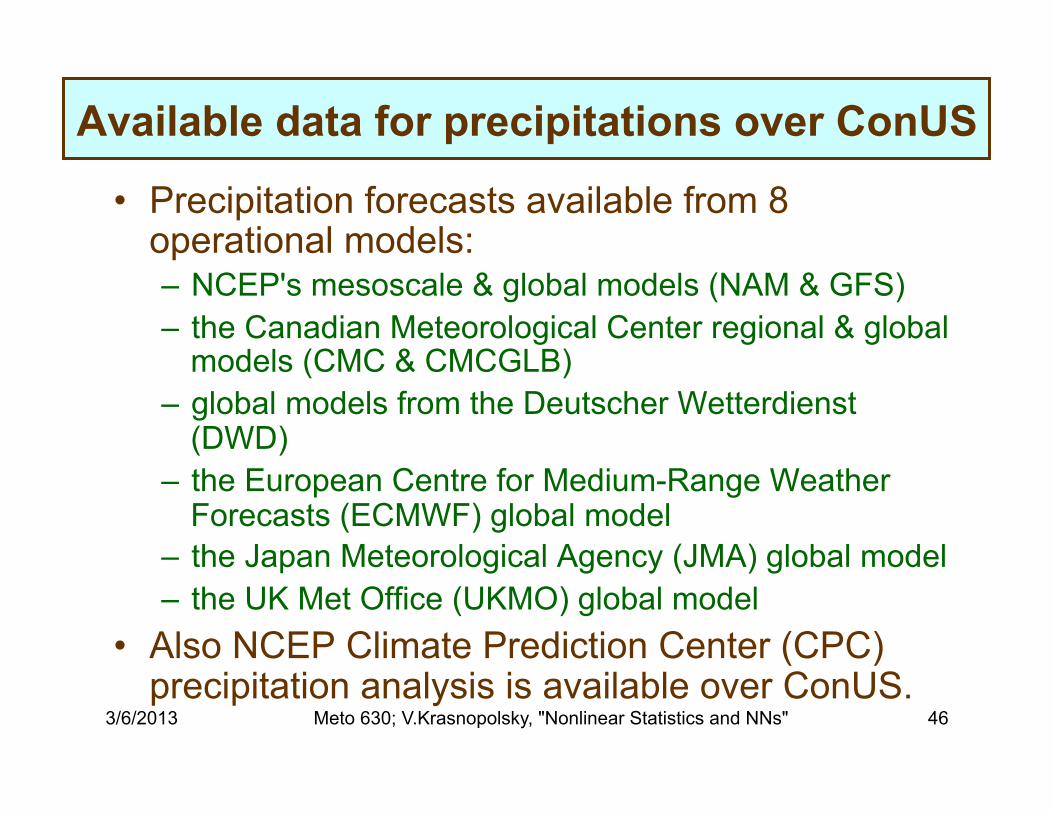
Available data for precipitations over ConUS
• Precipitation forecasts available from 8 operational models: – NCEP's mesoscale & global models (NAM & GFS) – the Canadian Meteorological Center regional & global
models (CMC & CMCGLB) – global models from the Deutscher Wetterdienst
(DWD) – the European Centre for Medium-Range Weather
Forecasts (ECMWF) global model – the Japan Meteorological Agency (JMA) global model – the UK Met Office (UKMO) global model
• Also NCEP Climate Prediction Center (CPC) precipitation analysis is available over ConUS.
3/6/2013 Meto 630; V.Krasnopolsky, "Nonlinear Statistics and NNs" 47
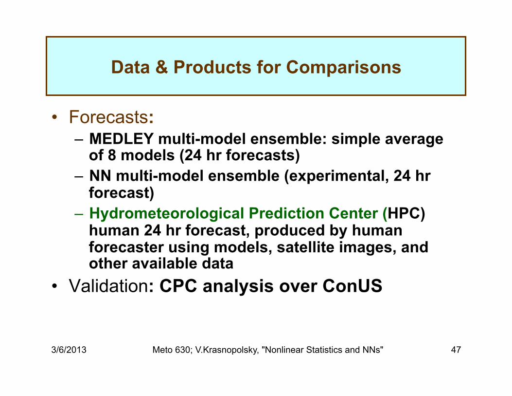
Data & Products for Comparisons
• Forecasts: – MEDLEY multi-model ensemble: simple average
of 8 models (24 hr forecasts) – NN multi-model ensemble (experimental, 24 hr
forecast) – Hydrometeorological Prediction Center (HPC)
human 24 hr forecast, produced by human forecaster using models, satellite images, and other available data
• Validation: CPC analysis over ConUS
3/6/2013 Meto 630; V.Krasnopolsky, "Nonlinear Statistics and NNs" 48
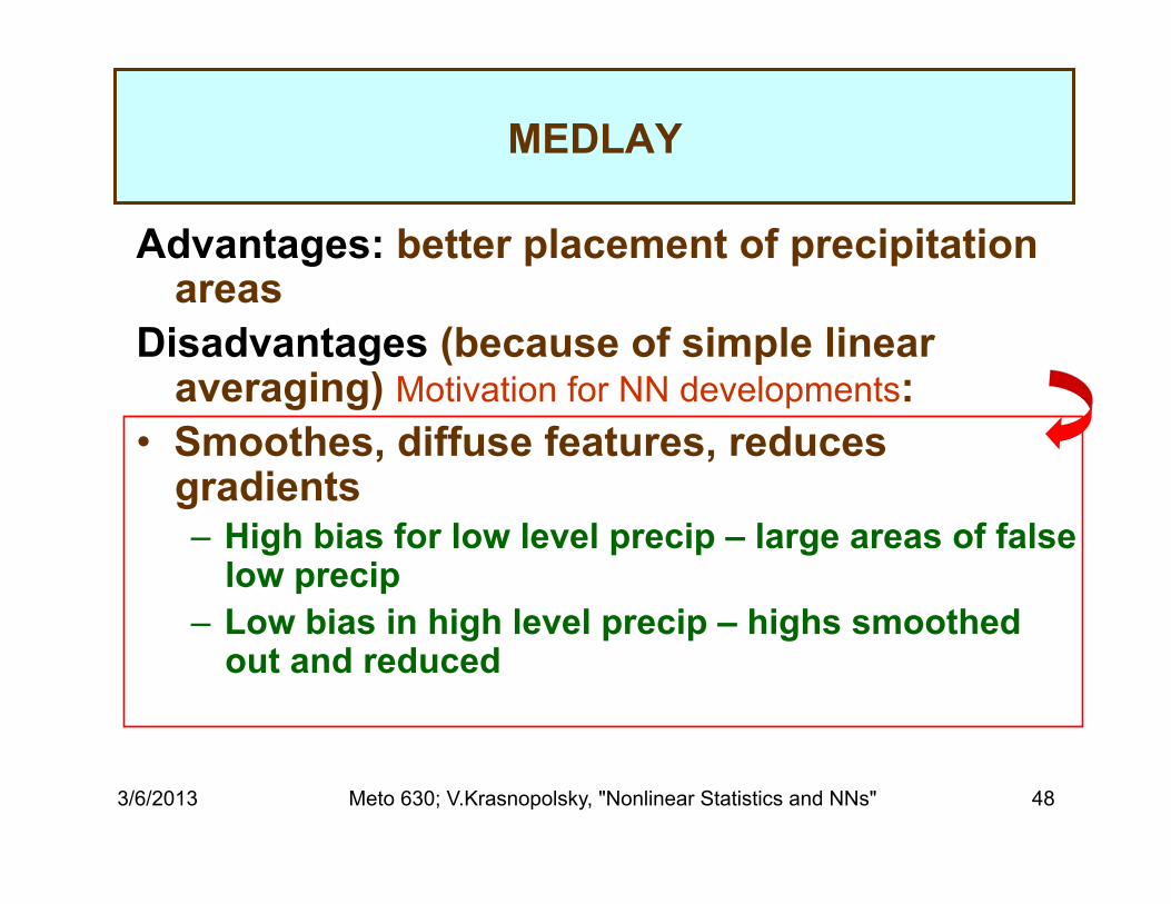
Advantages: better placement of precipitation areas
Disadvantages (because of simple linear averaging) Motivation for NN developments:
• Smoothes, diffuse features, reduces gradients – High bias for low level precip – large areas of false
low precip – Low bias in high level precip – highs smoothed
out and reduced
MEDLAY

3/6/2013 Meto 630; V.Krasnopolsky, "Nonlinear Statistics and NNs" 49
Verifying CPC analysis
MEDLEY
NAM
GFS
24h Forecast Ending 07/24/2010 at 12Z

3/6/2013 Meto 630; V.Krasnopolsky, "Nonlinear Statistics and NNs" 50
A NN Multi-Model Ensemble
• Use past data (model forecasts and verifying analysis data) to train NN – For NN Inputs: precip amounts (8 model 24 hr
forecasts), lat, lon, and day of the year – For NN output: CPC verification analysis for the
corresponding time • Data for 2009 have been used for training
; n = 12; k = 7 ∑ ∑
= =
⋅+⋅+=k
j
n
iijijjens xbbaaNN
1 100 )(φ

3/6/2013 Meto 630; V.Krasnopolsky, "Nonlinear Statistics and NNs" 51
Verifying CPC analysis GFS
NAM ECMWF
Sample NN forecast: example 1 (1)
3/6/2013 Meto 630; V.Krasnopolsky, "Nonlinear Statistics and NNs" 52
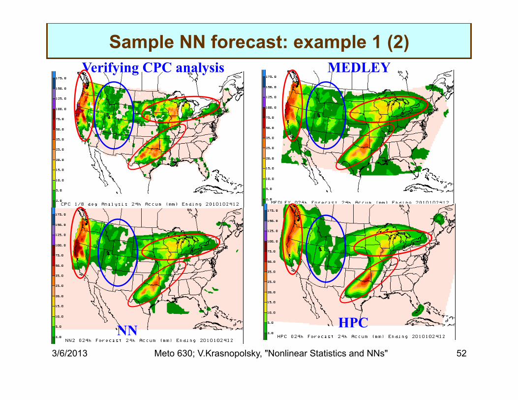
Verifying CPC analysis MEDLEY
NN HPC
Sample NN forecast: example 1 (2)

3/6/2013 Meto 630; V.Krasnopolsky, "Nonlinear Statistics and NNs" 53
Verifying CPC analysis MEDLEY
NN HPC
Sample NN forecast: example 2
3/6/2013 Meto 630; V.Krasnopolsky, "Nonlinear Statistics and NNs" 54
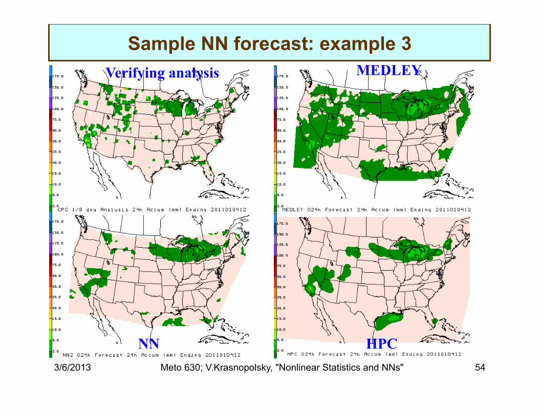
Verifying analysis
HPC NN
MEDLEY
Sample NN forecast: example 3
3/6/2013 Meto 630; V.Krasnopolsky, "Nonlinear Statistics and NNs" 55
Application of the Neural Network Technique to Develop New NN Convection
Parameterization
3/6/2013 Meto 630; V.Krasnopolsky, "Nonlinear Statistics and NNs" 56
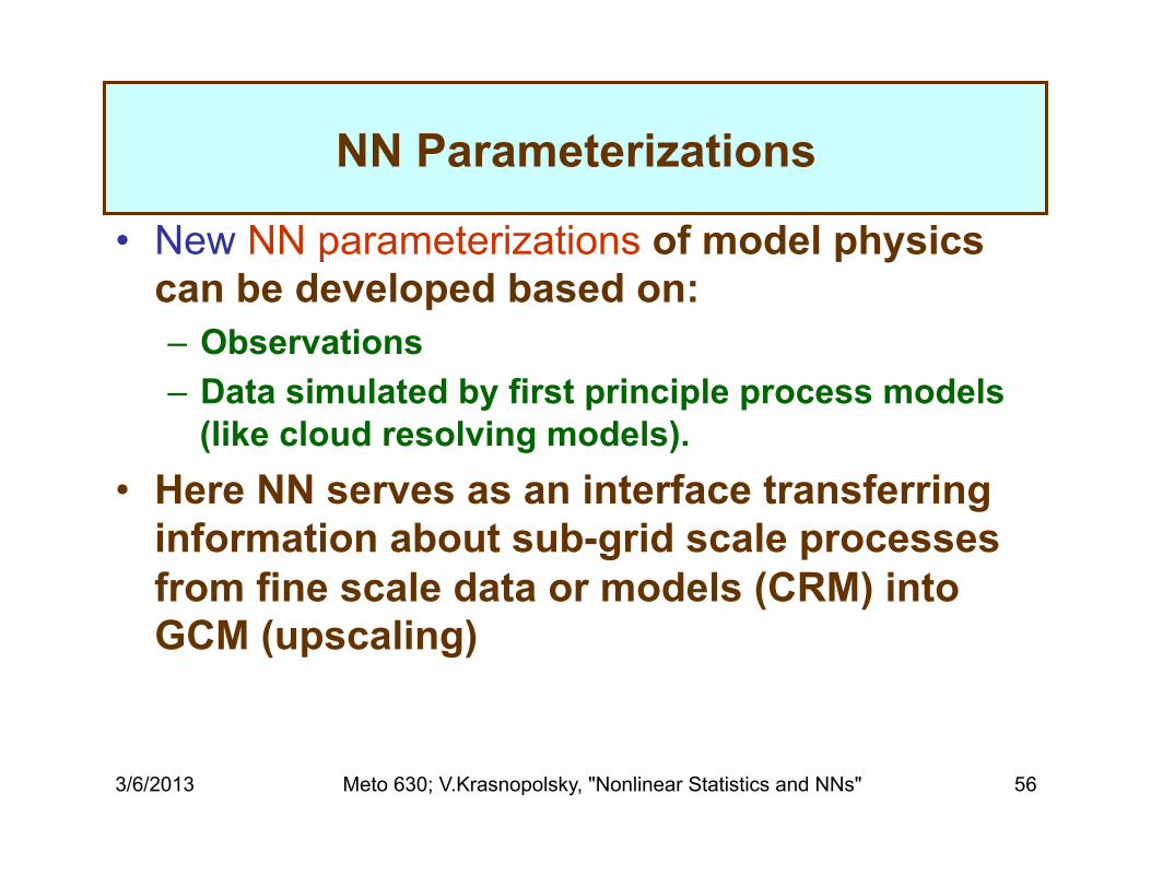
NN Parameterizations
• New NN parameterizations of model physics can be developed based on: – Observations – Data simulated by first principle process models
(like cloud resolving models). • Here NN serves as an interface transferring
information about sub-grid scale processes from fine scale data or models (CRM) into GCM (upscaling)

3/6/2013 Meto 630; V.Krasnopolsky, "Nonlinear Statistics and NNs" 57
NN convection parameterizations for climate models based on learning from data.
Proof of Concept (POC) -1.
Data
CRM 1 x 1 km 96 levels
T & Q Reduce Resolution to ~250 x 250 km
26 levels
Prec., Tendencies, etc. Reduce Resolution to ~250 x 250 km
26 levels
NN
Training Set
Initialization Forcing
“Pseudo- Observations”
3/6/2013 Meto 630; V.Krasnopolsky, "Nonlinear Statistics and NNs" 58
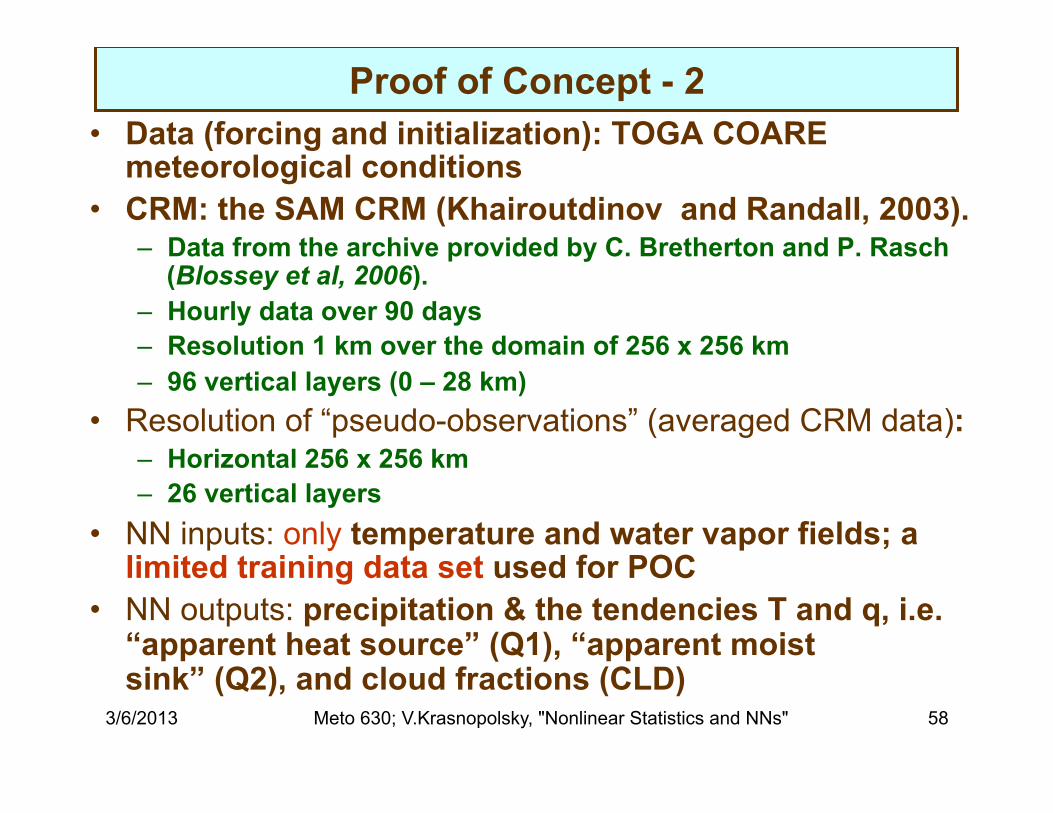
Proof of Concept - 2 • Data (forcing and initialization): TOGA COARE
meteorological conditions • CRM: the SAM CRM (Khairoutdinov and Randall, 2003).
– Data from the archive provided by C. Bretherton and P. Rasch (Blossey et al, 2006).
– Hourly data over 90 days – Resolution 1 km over the domain of 256 x 256 km – 96 vertical layers (0 – 28 km)
• Resolution of “pseudo-observations” (averaged CRM data): – Horizontal 256 x 256 km – 26 vertical layers
• NN inputs: only temperature and water vapor fields; a limited training data set used for POC
• NN outputs: precipitation & the tendencies T and q, i.e. “apparent heat source” (Q1), “apparent moist sink” (Q2), and cloud fractions (CLD)

3/6/2013 Meto 630; V.Krasnopolsky, "Nonlinear Statistics and NNs" 59
Time averaged water vapor tendency (expressed as the equivalent heating) for the validation dataset.
Q2 profiles (red) with the corresponding NN generated profiles (blue). The profile rmse increases from the left to the right.
Proof of Concept - 4

3/6/2013 Meto 630; V.Krasnopolsky, "Nonlinear Statistics and NNs" 60
Proof of Concept - 3
Precipitation rates for the validation dataset. Red – data, blue - NN

3/6/2013 Meto 630; V.Krasnopolsky, "Nonlinear Statistics and NNs" 61
How to Develop NNs: An Outline of the Approach (1)
• Problem Analysis: – Are traditional approaches unable to solve your problem?
• At all • With desired accuracy • With desired speed, etc.
– Are NNs well-suited for solving your problem? • Nonlinear mapping • Classification • Clusterization, etc.
– Do you have a first guess for NN architecture? • Number of inputs and outputs • Number of hidden neurons
3/6/2013 Meto 630; V.Krasnopolsky, "Nonlinear Statistics and NNs" 62
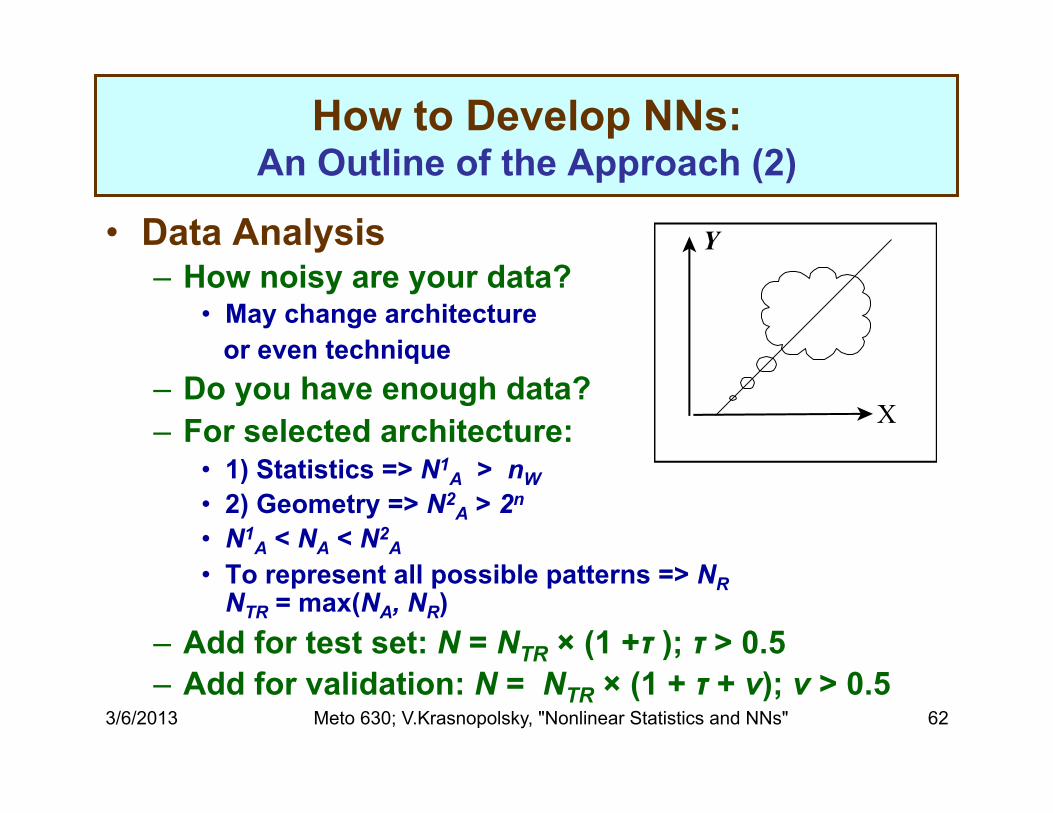
How to Develop NNs: An Outline of the Approach (2)
• Data Analysis – How noisy are your data?
• May change architecture or even technique
– Do you have enough data? – For selected architecture:
• 1) Statistics => N1A > nW
• 2) Geometry => N2A > 2n
• N1A < NA < N2
A • To represent all possible patterns => NR
NTR = max(NA, NR) – Add for test set: N = NTR × (1 +τ ); τ > 0.5 – Add for validation: N = NTR × (1 + τ + ν); ν > 0.5
Y
X

3/6/2013 Meto 630; V.Krasnopolsky, "Nonlinear Statistics and NNs" 63
How to Develop NNs: An Outline of the Approach (3)
• Training – Try different initializations – If results are not satisfactory, then goto Data
Analysis or Problem Analysis • Validation (must for any nonlinear tool!)
– Apply trained NN to independent validation data – If statistics are not consistent with those for
training and test sets, go back to Training or Data Analysis

3/6/2013 Meto 630; V.Krasnopolsky, "Nonlinear Statistics and NNs" 64
Conclusions • There is an obvious trend in scientific studies:
– From simple, linear, single-disciplinary, low dimensional systems
– To complex, nonlinear, multi-disciplinary, high dimensional systems
• There is a corresponding trend in math & statistical tools: – From simple, linear, single-disciplinary, low dimensional
tools and models – To complex, nonlinear, multi-disciplinary, high dimensional
tools and models • Complex, nonlinear tools have advantages &
limitations: learn how to use advantages & avoid limitations!
• Check your toolbox and follow the trend, otherwise you may miss the train!
3/6/2013 Meto 630; V.Krasnopolsky, "Nonlinear Statistics and NNs" 65
Recommended Reading • Regression Models:
– B. Ostle and L.C. Malone, “Statistics in Research”, 1988 • NNs, Introduction:
– R. Beale and T. Jackson, “Neural Computing: An Introduction”, 240 pp., Adam Hilger, Bristol, Philadelphia and New York., 1990
• NNs, Advanced: – Bishop Ch. M., 2006: Pattern Recognition and Machine Learning, Springer. – V. Cherkassky and F. Muller, 2007: Learning from Data: Concepts, Theory,
and Methods, J. Wiley and Sons, Inc – Haykin, S. (1994), Neural Networks: A Comprehensive Foundation, 696 pp.,
Macmillan College Publishing Company, New York, U.S.A. – Ripley, B.D. (1996), Pattern Recognition and Neural Networks, 403 pp.,
Cambridge University Press, Cambridge, U.K. – Vapnik, V.N., and S. Kotz (2006), Estimation of Dependences Based on
Empirical Data (Information Science and Statistics), 495 pp., Springer, New York.
• NNs in Environmental Sciences: – Krasnopolsky, V., 2007: “Neural Network Emulations for Complex
Multidimensional Geophysical Mappings: Applications of Neural Network Techniques to Atmospheric and Oceanic Satellite Retrievals and Numerical Modeling”, Reviews of Geophysics, 45, RG3009, doi:10.1029/2006RG000200.
– Hsieh, W., 2009: “Machine Learning Methods in the Environmental Sciences”, Cambridge University Press, 349 pp.