Introduction to Neutrino (Oscillation) Physics€¦ · Introduction to Neutrino (Oscillation)...

Introduction to Neutrino (Oscillation)Physics

Standard Model

of Particle Physics

Rodejohann/Schoening

17/07/13

1

Literature

• ArXiv:

– Bilenky, Giunti, Grimus: Phenomenology of Neutrino Oscillations,

hep-ph/9812360

– Akhmedov: Neutrino Physics, hep-ph/0001264

– Grimus: Neutrino Physics – Theory, hep-ph/0307149

• Textbooks:

– Fukugita, Yanagida: Physics of Neutrinos and Applications to

Astrophysics

– Kayser: The Physics of Massive Neutrinos

– Giunti, Kim: Fundamentals of Neutrino Physics and Astrophysics

– Schmitz: Neutrinophysik

2

Contents

I Basics

I1) Introduction

I2) History of the neutrino

I3) Fermion mixing, neutrinos and the Standard Model

3

Contents

II Neutrino Oscillations

II1) The PMNS matrix

II2) Neutrino oscillations in vacuum

II3) Results and their interpretation – what have we learned?

II4) Prospects – what do we want to know?

4

Contents

I Basics

I1) Introduction



5

I1) IntroductionStandard Model of Elementary Particle Physics: SU(3)C × SU(2)L × U(1)Y

uR

dR

cR

sR

tR

bR

eR

R

R

uL

dL

cL

sL

tL

bL

eL

L

Le

Species #∑

Quarks 10 10

Leptons 3 13

Charge 3 16

Higgs 2 18

18 free parameters. . .

+ Dark Matter

+ Gravitation

+ Dark Energy

+ Baryon Asymmetry

6

Standard Model of Elementary Particle Physics: SU(3)C × SU(2)L × U(1)Y

uR

dR

cR

sR

tR

bR

eR

R

R

uL

dL

cL

sL

tL

bL

eL

L

Le

Species #∑

Quarks 10 10

Leptons 3 13

Charge 3 16

Higgs 2 18

+ Neutrino Mass mν

7

Standard Model∗ of Particle Physics

add neutrino mass matrix mν (and a new energy scale?)

Species #∑

Quarks 10 10

Leptons 3 13

Charge 3 16

Higgs 2 18

8

Standard Model∗ of Particle Physics

add neutrino mass matrix mν (and a new energy scale?)

Species #∑

Quarks 10 10

Leptons 3 13

Charge 3 16

Higgs 2 18

−→

Species #∑

Quarks 10 10

Leptons 12 (10) 22 (20)

Charge 3 25 (23)

Higgs 2 27 (25)

Two roads towards more understanding: Higgs and Flavor

9

NEUTRINOS

LHCILC...

Baryon

...

GUT

SO(10) ...

BBN...

...

Supersymmetry

Astrophysics

cosmic rayssupernovae

Cosmology

Dark Matter

quark mixing

Flavor physics

proton decaysee−saw

Asymmetry

10

NEUTRINOS

LHCILC...

Baryon

...

GUT

SO(10) ...

BBN...

...

Astrophysics

cosmic rays

Supersymmetry

Cosmologie

Dark Matter

Asymmetry

Flavor physics

see−sawproton decay

quark mixing

supernovae

11

General Remarks

• Neutrinos interact weakly: can probe things not testable by other means

– solar interior

– geo-neutrinos

– cosmic rays

• Neutrinos have no mass in SM

– probe scales mν ∝ 1/Λ

– happens in GUTs

– connected to new concepts, e.g. Lepton Number Violation

⇒ particle and source physics

12

Contents

I Basics

I1) Introduction



13

I2) History

1926 problem in spectrum of β-decay

1930 Pauli postulates “neutron”

14

1932 Fermi theory of β-decay

1956 discovery of νe by Cowan and Reines (NP 1985)

1957 Pontecorvo suggests neutrino oscillations

1958 helicity h(νe) = −1 by Goldhaber ⇒ V −A

1962 discovery of νµ by Lederman, Steinberger, Schwartz (NP 1988)

1970 first discovery of solar neutrinos by Ray Davis (NP 2002); solar neutrino

problem

1987 discovery of neutrinos from SN 1987A (Koshiba, NP 2002)

1991 Nν = 3 from invisible Z width

1998 SuperKamiokande shows that atmospheric neutrinos oscillate

2000 discovery of ντ

2002 SNO solves solar neutrino problem

2010 the third mixing angle

15

Contents

I Basics

I1) Introduction



16

I3) Neutrinos and the Standard ModelSU(3)c × SU(2)L × U(1)Y → SU(3)c × U(1)em with Q = I3 +

12 Y

Le =

νe

e

L

∼ (1, 2,−1)

eR ∼ (1, 1,−2)

νR ∼ (1, 1, 0) total SINGLET!!

uR

dR

cR

sR

tR

bR

eR

R

R

uL

dL

cL

sL

tL

bL

eL

L

Le

17

Mass Matrices

3 generations of quarks

L′1 =

u′

d′

L

, L′2 =

c′

s′

L

, L′3 =

t′

b′

L

u′R , c′R , t

′R ≡ u′i,R and d′R , s

′R , b

′R ≡ d′i,R

gives mass term

−LY =∑

i,j

L′i

[

g(d)ij Φ d′j,R + g

(u)ij Φu′j,R

]

EWSB−→ ∑

i,j

v√2g(d)ij d′i,L d

′j,R + v√

2g(u)ij u′i,L u

′j,R

= d′LM(d) d′R + u′LM

(u) u′R

arbitrary complex 3× 3 matrices in “flavor (interaction, weak) basis”

18

Diagonalization

U †d M

(d) Vd = D(d) = diag(md,ms,mb)

U †uM

(u) Vu = D(u) = diag(mu,mc,mt)

with unitary matrices Uu,dU†u,d = U †

u,dUu,d = Vu,dV†u,d = V †

u,dVu,d = 1

in Lagrangian:

−LY = d′LM(d) d′R + u′LM

(u) u′R

d′L Ud︸︷︷︸

U †d M

(d) Vd︸︷︷︸

V †d d

′R

︸︷︷︸+ u′L Uu

︸︷︷︸U †uM

(u) Vu︸︷︷︸

V †u u

′R

︸︷︷︸

dL D(d) dR uL D(u) uR

physical (mass, propagation) states uL =

u

c

t

L

19

in interaction terms:

−LCC = g√2W+

µ u′L γµ d′L

g√2W+

µ u′L Uu︸︷︷︸

γµ U †u Ud︸︷︷︸

U †d d

′L

︸︷︷︸

uL V dL

Cabibbo-Kobayashi-Maskawa (CKM) matrix survives:

V = U †u Ud

Structure in Wolfenstein-parametrization:

V =

Vud Vus Vub

Vcd Vcs Vcb

Vtd Vts Vtb

=

1− λ2

2 λ Aλ3 (ρ− i η)

−λ 1− λ2

2 Aλ2

Aλ3 (1− ρ− i η) −Aλ2 1

with λ = sin θC = 0.22535± 0.00065, A = 0.811+0.022−0.012,

ρ = (1− λ2

2 ) ρ = 0.131+0.026−0.013, η = 0.345+0.013

−0.014

20

Lesson to learn:

|V | =

0.97427± 0.00015 0.22534± 0.000065 0.00351+0.00015−0.00014

0.22520± 0.000065 0.97344± 0.00016 0.0412+0.0011−0.0005

0.00867+0.00029−0.00031 0.0404+0.0011

−0.0005 0.999146+0.000021−0.000046

small mixing in the quark sector

related to hierarchy of masses?

M =

0 a

a b

= U DUT with U =

cos θ sin θ

− sin θ cos θ

where D = diag(m1,m2)

from 11-entry one gets

tan θ =

√m1

m2

compare with√

md/ms ≃ 0.22 and tan θC ≃ 0.23

21

Number of parameters in V for N families:

complex N ×N 2N2 2N2

unitarity −N2 N2

rephase ui, di −(2N − 1) (N − 1)2

a real matrix would have 12 N (N − 1) rotations around ij-axes

in total:

families angles phases

2 1 0

3 3 1

4 6 3

N 12 N (N − 1) 1

2 (N − 2) (N − 1)

22

Masses in the SM:

−LY = ge LΦ eR + gν L Φ νR + h.c.

with

L =

νe

e

L

and Φ = iτ2 Φ∗ = iτ2

φ+

φ0

∗

=

φ0

−φ+

∗

after EWSB: 〈Φ〉 → (0, v/√2)T and 〈Φ〉 → (v/

√2, 0)T

−LY = gev√2eL eR + gν

v√2νL νR + h.c. ≡ me eL eR +mν νL νR + h.c.

⇔ in a renormalizable, lepton number conserving model with Higgs doublets the

absence of νR means absence of mν

23

Lepton Masses

−LY = e′LM(ℓ) e′R

=e′L Uℓ︸︷︷︸

U †ℓ M

(ℓ) Vℓ︸︷︷︸

V †ℓ e

′R

︸︷︷︸

eL D(ℓ) eR

and in charged current term:

−LCC = g√2W+

µ e′L γµ ν′L

g√2W+

µ e′L Uℓ︸︷︷︸

γµ U †ℓ Uν︸︷︷︸

U †ν ν

′L

︸︷︷︸

eL U νL

Rotation of νL is arbitrary in absence of mν : choose Uν = Uℓ

⇒ Pontecorvo-Maki-Nakagawa-Saki (PMNS) matrix

U = 1 for massless neutrinos!!

⇒ individual lepton numbers Le, Lµ, Lτ are conserved

24

Contents






25


Neutrinos have mass, so:

−LCC =g√2ℓL γ

µ U νLW−µ with U = U †

ℓ Uν

Pontecorvo-Maki-Nakagawa-Sakata (PMNS) matrix

να = U∗αi νi

connects flavor states να (α = e, µ, τ) to mass states νi (i = 1, 2, 3)

26

Number of parameters in U for N families:


unitarity −N2 N2

rephase νi, ℓi −(2N − 1) (N − 1)2


in total:

families angles phases

2 1 0

3 3 1

4 6 3

N 12 N (N − 1) 1

2 (N − 2) (N − 1)

this assumes νν mass term, what if νT ν ?

27

Number of parameters in U for N families:


unitarity −N2 N2

rephase ℓα −N N(N − 1)


in total:

families angles phases extra phases

2 1 1 1

3 3 3 2

4 6 6 3

N 12 N (N − 1) 1

2 N (N − 1) N − 1

Extra N − 1 “Majorana phases” because of mass term νT ν

(absent for Dirac neutrinos)

28

Majorana Phases

• connected to Majorana nature, hence to Lepton Number Violation

• I can always write: U = U P , where all Majorana phases are in

P = diag(1, eiφ1 , eiφ2 , eiφ3 , . . .):

• 2 families:

U =

cos θ sin θ

− sin θ cos θ

1 0

0 eiα

29

• 3 families: U = R23 R13R12 P

=

1 0 0

0 c23 s23

0 −s23 c23

c13 0 s13 e−iδ

0 1 0

−s13 eiδ 0 c13

c12 s12 0

−s12 c12 0

0 0 1

P

=

c12 c13 s12 c13 s13 eiδ

−s12 c23 − c12 s23 s13 e−iδ c12 c23 − s12 s23 s13 e

−iδ s23 c13

s12 s23 − c12 c23 s13 e−iδ −c12 s23 − s12 c23 s13 e

−iδ c23 c13

P

with P = diag(1, eiα, eiβ)

30

Dirac vs. Majorana neutrinos

why are neutrinos (probably) Majorana, why is their mass so small, how do I

show that neutrinos are Majorana, what does this mean for physics beyond the

Standard Model,. . .

See next term:-)

• MVSpec Standard Model II (Rodejohann + Lindner)

• MVSem Astroparticle Physics: Theory and Experiment (Rodejohann et al.)

31

Contents






32

Probability:

P (να → νβ , t) ≡ Pαβ = |A(να → νβ , t)|2

=∑

ij

U∗αi Uβi U

∗βj Uαj

︸︷︷︸e−i (Ei−Ej) t︸︷︷︸

J αβij e−i∆ij

= . . . =

Pαβ = δαβ − 4∑

j>i

Re{J αβij } sin2

∆ij

2+ 2

∑

j>i

Im{J αβij } sin∆ij

with phase

12∆ij =

12 (Ei − Ej) t ≃ 1

2

(√

p2i +m2i −

√

p2j +m2j

)

L

≃ 12

(

pi (1 +m2

i

2p2

i

)− pj (1 +m2

j

2p2

j

))

L ≃ m2

i−m2

j

4E L

1

2∆ij =

m2i −m2

j

4EL ≃ 1.27

(

∆m2ij

eV2

)(L

km

)(GeV

E

)

34

Pαβ = δαβ − 4∑

j>i

Re{J αβij } sin2

∆ij

2+ 2

∑

j>i


• α = β: survival probability

• α 6= β: transition probability

• requires U 6= 1 and ∆m2ij 6= 0

•∑

α

Pαβ = 1 ↔ conservation of probability

• J αβij invariant under Uαj → eiφα Uαj e

iφj

⇒ Majorana phases drop out!

35

CP Violation

In oscillation probabilities: U → U∗ for anti-neutrinos

Define asymmetries:

∆αβ = P (να → νβ)− P (να → νβ) = P (να → νβ)− P (νβ → να)

= 4∑

j>i


• 2 families: U is real and Im{J αβij } = 0 ∀α, β, i, j

• 3 families:

∆eµ = −∆eτ = ∆µτ =

(

sin∆m2

21

2EL+ sin

∆m232

2EL+ sin

∆m213

2EL

)

JCP

where JCP = Im{Ue1 Uµ2 U

∗e2 U

∗µ1

}

= 18 sin 2θ12 sin 2θ23 sin 2θ13 cos θ13 sin δ

vanishes for one ∆m2ij = 0 or one θij = 0 or δ = 0, π

36

• CP violation in survival probabilities vanishes:

P (να → να)− P (να → να) ∝∑

j>i

Im{J ααij } =

∑

j>i

Im{U∗αi Uαi U

∗αj Uαj} = 0

• Recall that U = U †ℓ Uν

If charged lepton masses diagonal, then mν is diagonalized by PMNS matrix:

mν = U diag(m1,m2,m3)UT

Define h = mν m†ν and find that

Im {h12 h23 h31} = ∆m221 ∆m

231 ∆m

232 JCP

37

Two Flavor Case

U =

Uα1 Uα2

Uβ1 Uβ2

=

cos θ sin θ

− sin θ cos θ

⇒ J αα12 = |Uα1|2|Uα2|2 =

1

4sin2 2θ

and transition probability is Pαβ = sin2 2θ sin2∆m2

21

4EL

38

• amplitude sin2 2θ

• maximal mixing for θ = π/4 ⇒ να =√

12 (ν1 + ν2)

• oscillation length Losc = 4π E/∆m221 = 2.48 E

GeVeV2

∆m221

km

⇒ Pαβ = sin2 2θ sin2 πL

Losc

is distance between two maxima (minima)

e.g.: E = GeV and ∆m2 = 10−3 eV2: Losc ≃ 103 km

40

(km/MeV)eν/E0L

20 30 40 50 60 70 80 90 100

Surv

ival

Pro

babi

lity

0

0.2

0.4

0.6

0.8

1

eνData - BG - Geo Expectation based on osci. parameters

determined by KamLAND

41

L≫ Losc: fast oscillations 〈sin2 πL/Losc〉 = 12

and Pαα = 1− 2 |Uα1|2 |Uα2|2 = |Uα1|4 + |Uα2|4

sensitivity to mixing

42

L≫ Losc: fast oscillations 〈sin2 πL/Losc〉 = 12

and Pαβ = 2 |Uα1|2 |Uα2|2 = |Uα1|2 |Uβ1|2 + |Uα2|2 |Uβ2|2 = 12 sin

2 2θ

sensitivity to mixing

43

L≪ Losc: hardly oscillations and Pαβ = sin2 2θ (∆m2L/(4E))2

sensitivity to product sin2 2θ∆m2

44

large ∆m2: sensitivity to mixing

small ∆m2: sensitivity to sin2 2θ∆m2

maximal sensitivity when ∆m2L/E ≃ 2π

45

Characteristics of typical oscillation experiments

Source Flavor E [GeV] L [km] (∆m2)min [eV2]

Atmosphere(−)νe ,

(−)νµ 10−1 . . . 102 10 . . . 104 10−6

Sun νe 10−3 . . . 10−2 108 10−11

Reactor SBL νe 10−4 . . . 10−2 10−1 10−3

Reactor LBL νe 10−4 . . . 10−2 102 10−5

Accelerator LBL(−)νe ,

(−)νµ 10−1 . . . 1 102 10−1

Accelerator SBL(−)νe ,

(−)νµ 10−1 . . . 1 1 1

46

Quantum Mechanics

Can’t distinguish the individual mi: coherent sum of amplitudes and interference

47

Quantum Mechanics

Textbook calculation is completely wrong!!

• Ei − Ej is not Lorentz invariant

• massive particles with different pi and same E violates energy and/or

momentum conservation

• definite p: in space this is eipx, thus no localization

48

Quantum Mechanics

consider Ej and pj =√

E2j −m2

j :

pj ≃ E +m2j

∂pj∂m2

j

∣∣∣∣∣mj=0

≡ E − ξm2

j

2E, with ξ = −2E

∂pj∂m2

j

∣∣∣∣∣mj=0

Ej ≃ pj +m2j

∂Ej

∂m2j

∣∣∣∣∣mj=0

= pj +m2

j

2pj= E +

m2j

2E(1− ξ)

in pion decay π → µν:

Ej =m2

π

2

(

1−m2

µ

m2π

)

+m2

j

2m2π

thus,

ξ =1

2

(

1 +m2

µ

m2π

)

≃ 0.8 in Ei − Ej ≃ (1− ξ)∆m2

ij

2E

49

wave packet with size σx(>∼ 1/σp) and group velocity vi = ∂Ei/∂pi = pi/Ei:

ψi ∝ exp

{

−i(Ei t− pi x)−(x− vi t)

2

4σ2x

}

1) wave packet separation should be smaller than σx!

L∆v < σx ⇒ L

Losc<

p

σp

(loss of coherence: interference impossible)

2) m2ν should NOT be known too precisely!

if known too well: ∆m2 ≫ δm2ν =

∂m2ν

∂pνδpν ⇒ δxν ≫ 2 pν

∆m2=Losc

2π

(I know which state νi is exchanged, localization)

In both cases: Pαα = |Uα1|4 + |Uα2|4 (same as for L≫ Losc)

50

Quantum Mechanics

total amplitude for α→ β should be given by

A ∝∑

j

∫d3p

2Ej

A∗βj Aαj exp {−i(Ejt− px)}

with production and detection amplitudes

Aαj A∗βj ∝ exp

{

− (p− pj)2

4σ2p

}

we expand around pj :

Ej(p) ≃ Ej(pj) +∂Ej(p)

∂p

∣∣∣∣p=pj

(p− pj) = Ej + vj (p− pj)

and perform the integral over p:

A ∝∑

j

exp

{

−i(Ejt− pjx)−(x− vjt)

2

4σ2x

}

51

the probability is the integral of |A|2 over t:

P =

∫

dt |A|2 ∝ exp

{

−i[

(Ej − Ek)vj + vkv2j + v2k

− (pj − pk)

]

x

}

× exp

{

− (vj − vk)2x2

4σ2x(v

2j + v2k)

− (Ej − Ek)2

4σ2p(v

2j + v2k)

}

now express average momenta, energy and velocity as

pj ≃ E − ξm2

j

2E

Ej ≃ E + (1− ξ)m2

j

2E, vj =

pj

Ej

≃ 1−m2

j

2E2

this we insert in first exponential of P :[

(Ej − Ek)vj + vkv2j + v2k

− (pj − pk)

]

=∆m2

jkL

2E

52

the second exponential (damping term) can also be rewritten and the final

probability is

P ∝ exp

−i

∆m2ij

2EL−

(

L

Lcohjk

)2

− 2π2(1− ξ)2

(

σxLoscjk

)2

with

Lcohjk =

4√2E2

|∆m2jk|σx and Losc

jk =4πE

|∆m2jk|

expressing the two conditions (coherence and localization) for oscillation

discussed before

53

Contents






54

II3) Results and their interpretation – what have welearned?

• Main results as by-products:

– check solar fusion in Sun → solar neutrino problem

– look for nucleon decay → atmospheric neutrino oscillations

• almost all current data described by 2-flavor formalism

• sophisticated: confirm genuine 3-flavor effects:

– third mixing angle

– mass ordering

– CP violation

• have entered precision era

55

Interpretation in 3 Neutrino Framework

assume ∆m221 ≪ ∆m2

31 ≃ ∆m232 and small θ13:

• atmospheric and accelerator neutrinos: ∆m221L/E ≪ 1

P (νµ → ντ ) ≃ sin2 2θ23 sin2∆m2

31

4EL

• solar and KamLAND neutrinos: ∆m231L/E ≫ 1

P (νe → νe) ≃ 1− sin2 2θ12 sin2∆m2

21

4EL

• short baseline reactor neutrinos: ∆m221L/E ≪ 1

P (νe → νe) ≃ 1− sin2 2θ13 sin2∆m2

31

4EL

56

Solar Neutrinos

98% of energy production in fusion of net reaction

4 p+ 2 e− →4He++ + 2 νe + 26.73 MeV

26 MeV of the energy go in photons, i.e., 13 MeV per νe;

get neutrino flux from solar constant

S = 8.5× 1011 MeVcm−2 s−1 ⇒ Φν =S

13 MeV= 6.5× 1010 cm−2 s−1

57

Solar Standard Model (SSM) predicts 5 sources of neutrinos from pp-chain

Bahcall et al.

58

Different experiments sensitive to different energy, hence different neutrinos

• Homestake: νe +37Cl → 37Ar + e−

• Gallex, GNO, SAGE: νe +71Ga → 71Ge + e−

• (Super)Kamiokande: νe + e− → νe + e−

All find less neutrinos than predicted by SSM, deficit is energy dependent:

“solar neutrino problem”

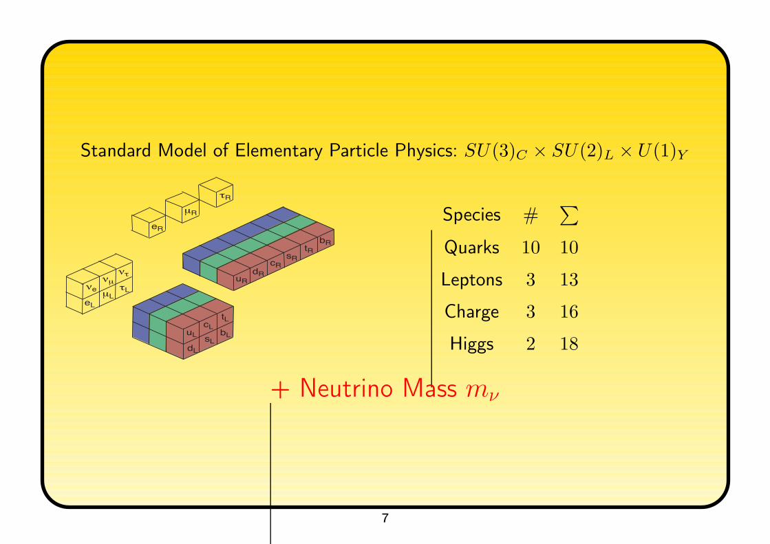
Breakthrough came with SNO experiment, using heavy water

59

charged current: Φ(νe)

neutral current: Φ(νe) + Φ(νµτ )

elastic scattering: Φ(νe) + 0.15Φ(νµτ )

61

0 1 2 3 4 5 60

1

2

3

4

5

6

7

8

)-1 s-2 cm6

(10eφ

)-1

s-2

cm

6 (

10

τµ

φ SNONCφ

SSMφ

SNOCCφSNO

ESφ

62

Results of fits give

sin2 θ12 ≃ 0.30

∆m221 ≡ ∆m2

⊙ ≃ 8× 10−5 eV2

only works with matter effects and resonance in Sun

⇒ ∆m2⊙ cos 2θ12 = (m2

2 −m21) (cos

2 θ12 − sin2 θ12) > 0

choosing cos 2θ12 > 0 fixes ∆m2⊙ > 0

63

low E: Pee = 1− 12 sin

2 2θ12 ≃ 59

large E: Pee = sin2 θ12 = 13

64

∆m

2 in e

V2 x10-4

0

1

sin2(Θ)

0.2 0.3 0.4

∆m

2 in e

V2

x10-5

6

7

8

9

sin2(Θ)

0.2 0.3 0.4

KamLAND: reactor neutrinos

n→ p+ e− + νe with E ≃ few MeV

If L ≃ 100 km:

∆m2⊙

EL ∼ 1 ⇒ solar ν parameters!!

65

νe + p→ n+ e+ with Eν ≃ Eprompt + Erecoiln + 0.8 MeV

200 µs later: n+ p→ d+ γ

66

Neutrinos do oscillate

(km/MeV)eν/E0L

20 30 40 50 60 70 80 90 100

Surv

ival

Pro

babi

lity

0

0.2

0.4

0.6

0.8

1

eνData - BG - Geo Expectation based on osci. parameters

determined by KamLAND

KamLAND

67

Atmospheric Neutrinos

zenith angle cos θ = 1 L ≃ 500 km

zenith angle cos θ = 0 L ≃ 10 km down-going

zenith angle cos θ = −1 L ≃ 104 km up-going

68

SuperKamiokande

69

Atmospheric Neutrinos

Dip at L/E ≃ 500 km/GeV ⇒ Oscillatory Behavior!!

(3.8 σ evidence for ντ appearence)

72

Testing Atmospheric Neutrinos with Accelerators: K2K, MINOS,

T2K, OPERA, NoνA

Proton beam

p+X → π± , K± → π± →(−)νµ with E ≃ GeV

If L ≃ 100 km:

∆m2A

EL ∼ 1 ⇒ atmospheric ν parameters!!

P (νµ → νµ) = 1− sin2 2θ23 sin2∆m2

31

4EL

73

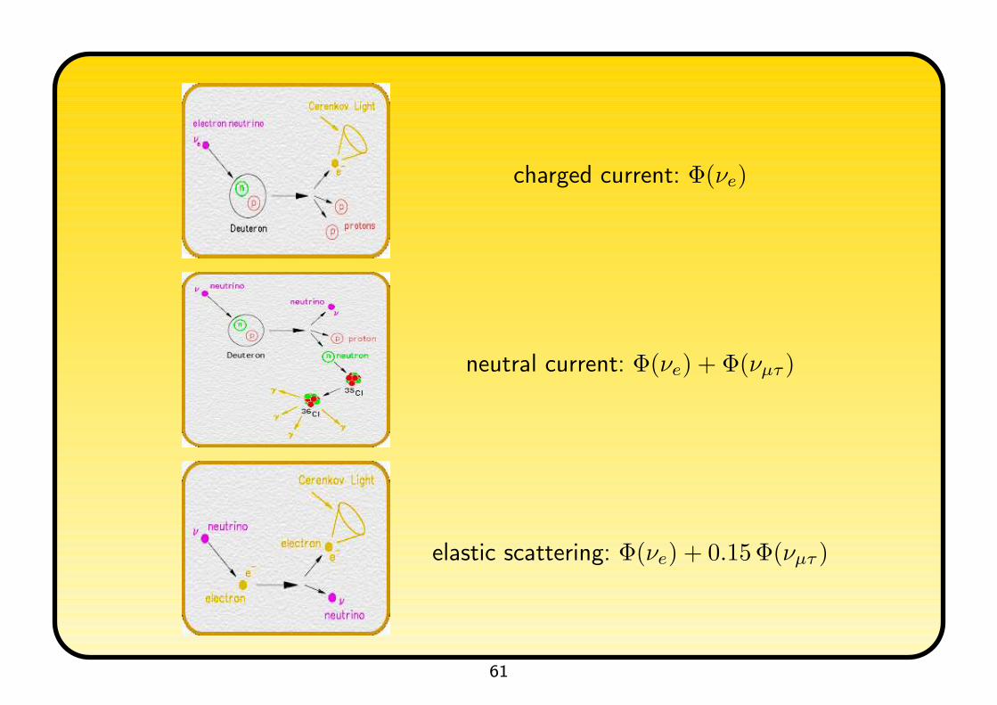
)θ(22) or sinθ(22sin0.6 0.7 0.8 0.9 1

)2 e

V-3

| (1

02

m∆| o

r |

2m∆|

1

2

3

4

5

1

2

3

4

5

MINOS 90% C.L. 2009-2011µν 2009-2010µν 2010-2011µν 2005-2010µν

90% C.L.µνSuper-K

Results of fits give

sin2 θ23 ≃ 0.50 maximal mixing?!

|∆m231| ≡ ∆m2

A ≃ 2.5× 10−3 eV2 ≃ 30∆m2⊙

NEW TREND (2012): less-than-maximal θ23?

74

Non-maximal θ23?

LBL accelerator experiments have octant-asymmetric amplitude (plus higher

order terms with sensitivity to δ and sgn(∆m2A))

P (νµ → νµ) ∝ cos2 θ13 sin2 θ23 (1− cos2 θ13 sin

2 θ23)

P (νµ → νe) ∝ cos2 θ13 sin2 θ13 sin

2 θ23

MINOS and T2K disappearence data most important, preference for θ23 6= π/4

atmospheric data:

Ne −N0e ∝ (R sin2 θ23 − 1) f(∆m2

A, θ13) + (R cos2 θ23 − 1) g(∆m2⊙, θ12)

−C sin θ13 sin θ23 cos θ23 cos δ

slight electron excess in sub-GeV atmospheric data sets easier explained by

cos δ = −1 and θ23 < π/4

75

The third mixing: Short-Baseline Reactor Neutrinos

Eν ≃ MeV and L ≃ 0.1 km:

∆m2A

E L ∼ 1 ⇒ atmospheric ν parameters!!

Pee = 1− sin2 2θ13 sin2∆m2

A

4E L

76

3 families: U = R23 R13R12 P

=

1 0 0

0 c23 s23

0 −s23 c23

c13 0 s13 e−iδ

0 1 0

−s13 eiδ 0 c13

c12 s12 0

−s12 c12 0

0 0 1

P

=

c12 c13 s12 c13 s13 eiδ

−s12 c23 − c12 s23 s13 e−iδ c12 c23 − s12 s23 s13 e

−iδ s23 c13

s12 s23 − c12 c23 s13 e−iδ −c12 s23 − s12 c23 s13 e

−iδ c23 c13

P

with P = diag(1, eiα, eiβ)

77

U =

c12 c13 s12 c13 s13 eiδ

−s12 c23 − c12 s23 s13 e−iδ c12 c23 − s12 s23 s13 e

−iδ s23 c13

s12 s23 − c12 c23 s13 e−iδ

−c12 s23 − s12 c23 s13 e−iδ c23 c13

=

1 0 0

0 c23 s23

0 −s23 c23

︸︷︷︸

c13 0 s13 e−iδ

0 1 0

−s13 eiδ 0 c13

︸︷︷︸

c12 s12 0

−s12 c12 0

0 0 1

︸︷︷︸

atmospheric and SBL reactor solar and

LBL accelerator LBL reactor

78

U =

c12 c13 s12 c13 s13 eiδ

−s12 c23 − c12 s23 s13 e−iδ c12 c23 − s12 s23 s13 e

−iδ s23 c13

s12 s23 − c12 c23 s13 e−iδ

−c12 s23 − s12 c23 s13 e−iδ c23 c13

=

1 0 0

0 c23 s23

0 −s23 c23

︸︷︷︸

c13 0 s13 e−iδ

0 1 0

−s13 eiδ 0 c13

︸︷︷︸

c12 s12 0

−s12 c12 0

0 0 1

︸︷︷︸

atmospheric and SBL reactor solar and

LBL accelerator LBL reactor

1 0 0

0√

1

2−

√1

2

0√

1

2

√1

2

1 0 0

0 1 0

0 0 1

√2

3

√1

30

−

√1

3

√2

30

0 0 1

(sin2 θ23 = 1

2) (sin2 θ13 = 0) (sin2 θ12 = 1

3)

∆m2

A∆m

2

A∆m2

⊙

79

Tri-bimaximal Mixing

approximation to PMNS matrix:

UTBM =

√23

√13 0

−√

16

√13 −

√12

−√

16

√13

√12

Harrison, Perkins, Scott (2002)

with mass matrix

(mν)TBM = U∗TBMmdiag

ν U †TBM =

A B B

· 12 (A+B +D) 1

2 (A+B −D)

· · 12 (A+B +D)

A =1

3

(2m1 +m2 e

−2iα), B =

1

3

(m2 e

−2iα −m1

), D = m3 e

−2iβ

⇒ Flavor symmetries. . .

80

Tri-bimaximal Mixing

UTBM =

√23

√13 0

−√

16

√13 −

√12

−√

16

√13

√12

Harrison, Perkins, Scott (2002)

This was still okay till end of 2010. . .

81

T2K: 2.5σ

p !"!

140m 0m 280m

off-axis

120m 295km280m0m

off-axis

110m

target

station decay

pipe

beam

dump

muon

monitors

280m

detectors

Super-Kamiokande

2.5o

P (νµ → νe) ≃ sin2 θ23 sin2 2θ13 sin

2 ∆m2A

4EL

normal inverted

82

More data

• MINOS: 1.7σ

• Double Chooz: 0.017 < sin2 2θ13 < 0.16 at 90 % C.L.

Pee = 1− sin2 2θ13 sin2∆m2

A

4EL

83

θ13: status

dominated by reactor experiments:

Double Chooz: sin2 2θ13 = 0.109± 0.030± 0.025 6= 0 at 2.9σ

Daya Bay: sin2 2θ13 = 0.089± 0.010± 0.005 6= 0 at 7.7σ

RENO: sin2 2θ13 = 0.113± 0.013± 0.019 6= 0 at 4.9σ

84

at least, Double Chooz are the only ones who made it to Big Bang Theory. . .

85

12θ 2sin0.25 0.30 0.35

0

1

2

3

4

23θ 2sin0.3 0.4 0.5 0.6 0.7

13θ 2sin0.01 0.02 0.03 0.04

2 eV-5/102mδ6.5 7.0 7.5 8.0 8.50

1

2

3

4

2 eV-3/102m∆2.0 2.2 2.4 2.6 2.8

π/δ0.0 0.5 1.0 1.5 2.0

oscillation analysisνSynopsis of global 3

σNσN

NHIH

86

What’s that good for?

1e-05 0.0001 0.001 0.01 0.1

sin2θ13

0

1

2

3

4

5

6

7

8

9

10

11

12N

umbe

r of M

odel

sanarchytexture zero SO(3)A

4

S3, S

4

Le-Lµ-Lτ

SRNDSO(10) lopsidedSO(10) symmetric/asym

Predictions of All 63 Models

↑

2025↑

2020↑

17/7/13

Albright, Chen

87

CKM vs. PMNS

|VCKM| ≃

0.974 0.225 0.004

0.225 0.973 0.041

0.009 0.040 0.999

|UPMNS| ≃

0.82 0.55 0.16

0.38 0.57 0.69

0.38 0.57 0.68

88

|U |2 ≃

0.795 . . . 0.846 0.513 . . . 0.585 0.126 . . . 0.178

0.205 . . . 0.543 0.416 . . . 0.730 0.579 . . . 0.808

0.215 . . . 0.548 0.409 . . . 0.725 0.567 . . . 0.800

• normal ordering: ∆m231 > 0

• inverted ordering: ∆m231 < 0

89

Contents



II2) Neutrino oscillations in vacuum and matter



90


9 physical parameters in mν

• θ12 and m22 −m2

1 (or θ⊙ and ∆m2⊙)

• θ23 and |m23 −m2

2| (or θA and ∆m2A)

• θ13 (or |Ue3|)

• m1, m2, m3

• sgn(m23 −m2

2)

• Dirac phase δ

• Majorana phases α and β (or α1 and α2, or φ1 and φ2, or. . .)

91

The future: open issues for neutrinos oscillations

Look for three flavor effects:

• precision measurements

– how maximal is θ23 ? how small/large is Ue3 ?

• sign of ∆m232 ?

tan 2θm = f(sgn(∆m2))

• is there CP violation?

• Problems:

– two small parameters: ∆m2⊙/∆m

2A ≃ 1/30 and |Ue3| <∼ 0.2

– 8-fold degeneracy for fixed L/E and νe → νµ channels

92

DegeneraciesExpand 3 flavor oscillation probabilities in terms of R = ∆m2

⊙/∆m2A and |Ue3|:

P (νe → νµ) ≃ sin2 2θ13 sin2 θ23sin2 (1−A)∆

(1−A)2+ R2 sin2 2θ12 cos2 θ23

sin2 A∆

A2

+sin δ sin 2θ13 R sin 2θ12 cos θ13 sin 2θ23 sin∆sin A∆ sin (1−A)∆

A(1−A)

+ cos δ sin 2θ13 R sin 2θ12 cos θ13 sin 2θ23 cos∆sin A∆ sin (1−A)∆

A(1−A)

with A = 2√2GF neE/∆m

2A and ∆ =

∆m2A

4E L

• θ23 ↔ π/2− θ23 degeneracy

• θ13-δ degeneracy

• δ-sgn(∆m2A) degeneracy

Solutions: more channels, different L/E, high precision,. . .

93

DegeneraciesExpand 3 flavor oscillation probabilities in terms of R = ∆m2

⊙/∆m2A and |Ue3|:


(1−A)2+ R2 sin2 2θ12 cos2 θ23

sin2 A∆

A2

+sin δ sin 2θ13 R sin 2θ12 cos θ13 sin 2θ23 sin∆sin A∆ sin (1−A)∆

A(1−A)

+ cos δ sin 2θ13 R sin 2θ12 cos θ13 sin 2θ23 cos∆sin A∆ sin (1−A)∆

A(1−A)

with A = 2√2GF neE/∆m

2A and ∆ =

∆m2A

4E L

If A∆ = π:


(1−A)2

This is the “magic baseline” of L =√2π

GF ne≃ 7500 km

94

Typical time scale

2005 2010 2015 2020 2025 2030Year

10-5

10-4

10-3

10-2

10-1

100

sin2 2Θ

13dis

cove

ryre

achH3ΣL

CHOOZ+Solar excluded

Branching pointConv. beams

Superbeams+Reactor exps

Superbeam upgrades

Ν-factories

MINOSCNGSD-CHOOZT2KNOîAReactor-IINOîA+FPD2ndGenPDExpNuFact

95

Future experiments

• what detector?

– Water Cerenkov?

– liquid scintillator?

– liquid argon?

• Neutrino Physics

– oscillations (hierarchy, CP, precision)

– non-standard physics (NSIs, unitarity violation, steriles, extra forces,. . .)

• other physics

– SN (burst and relic)

– geo-neutrinos

– p-decay

96

Example LBNE

FNAL → Homestake, L = 1300 km

97

Example ICAL at INO

7300 km from CERN, 6600 km from JHF at Tokai

99

Precision era!

∆m

2 in

eV

2

x10-5

6

7

8

9

sin2(Θ)

0.2 0.3 0.4

1998 today

100

Summary

101

Introduction to Neutrino (Oscillation) Physics€¦ · Introduction to Neutrino (Oscillation)...

Documents

Transcript of Introduction to Neutrino (Oscillation) Physics€¦ · Introduction to Neutrino (Oscillation)...