Introduction ToNeural Networks

• Development of Neural Networks date back to the early 1940s. It experienced an upsurge in popularity in the late 1980s. This was a result of the discovery of new techniques and developments and general advances in computer hardware technology.

• Some NNs are models of biological neural networks and some are not, but historically, much of the inspiration for the field of NNs came from the desire to produce artificial systems capable of sophisticated, perhaps ``intelligent", computations similar to those that the human brain routinely performs, and thereby possibly to enhance our understanding of the human brain.

• Most NNs have some sort of “training" rule. In other words, NNs “learn" from examples (as children learn to recognize dogs from examples of dogs) and exhibit some capability for generalization beyond the training data.

Neural Network Techniques

• Computers have to be explicitly programmed– Analyze the problem to be solved.– Write the code in a programming language.

• Neural networks learn from examples– No requirement of an explicit description of the problem.– No need a programmer.– The neural computer to adapt itself during a training period, based on

examples of similar problems even without a desired solution to each problem. After sufficient training the neural computer is able to relate the problem data to the solutions, inputs to outputs, and it is then able to offer a viable solution to a brand new problem.

– Able to generalize or to handle incomplete data.

NNs vs ComputersDigital Computers• Deductive Reasoning. We apply known

rules to input data to produce output.• Computation is centralized, synchronous,

and serial.• Memory is packetted, literally stored, and

location addressable.• Not fault tolerant. One transistor goes and

it no longer works.• Exact.• Static connectivity.

• Applicable if well defined rules with precise input data.

Neural Networks• Inductive Reasoning. Given input and

output data (training examples), we construct the rules.

• Computation is collective, asynchronous, and parallel.

• Memory is distributed, internalized, and content addressable.

• Fault tolerant, redundancy, and sharing of responsibilities.

• Inexact.• Dynamic connectivity.

• Applicable if rules are unknown or complicated, or if data is noisy or partial.

Evolution of Neural Networks• Realized that the brain could solve many

problems much easier than even the best computer– image recognition– speech recognition– pattern recognition

Very easy for the brain but very difficult for a computer

Evolution of Neural Networks• Studied the brain

– Each neuron in the brain has a relatively simple function

– But - 10 billion of them (60 trillion connections)

– Act together to create an incredible processing unit

– The brain is trained by its environment

– Learns by experience

Compensates for problems by massive parallelism

The Biological Inspiration

• The brain has been extensively studied by scientists.

• Vast complexity prevents all but rudimentary understanding.

• Even the behaviour of an individual neuron is extremely complex

• Engineers modified the neural models to make them more useful• less like biology• kept much of the terminology

The Structure of Neurons

axon

cell body

synapse

nucleus

dendrites

A neuron has a cell body, a branching input structure (the dendrite) and a branching output structure (the axon)• Axons connect to dendrites via synapses.• Electro-chemical signals are propagated from the dendritic input,

through the cell body, and down the axon to other neurons

• A neuron only fires if its input signal exceeds a certain amount (threshold) in a short time period.

• Synapses vary in strength– Good connections allowing a large signal– Slight connections allow only a weak signal.– Synapses either:

– Excitatory (stimulate)– Inhibitory (restrictive)

The Structure of Neurons

Biological Analogy

• Brain Neuron

• Artificial neuron(processing element)

• Set of processing elements (PEs) and connections (weights) with adjustable strengths

f(net)

Inpu

ts

w1

w2

wn

X4

X3

X5

X1

X2

OutputLayer

InputLayer

Hidden Layer

Benefits of Neural Networks

• Pattern recognition, learning, classification, generalization and abstraction, and interpretation of incomplete and noisy inputs

• Provide some human problem-solving characteristics

• Robust

• Fast, flexible and easy to maintain

• Powerful hybrid systems

(Artificial) Neural networks (ANN)

• ANN architecture

(Artificial) Neural networks (ANN)

• ‘Neurons’ – have 1 output but many inputs– Output is weighted sum of inputs– Threshold can be set

• Gives non-linear response

The Key Elements of Neural Networks

• Neural computing requires a number of neurons, to be connected together into a "neural network". Neurons are arranged in layers.

• Each neuron within the network is usually a simple processing unit which takes one or more inputs and produces an output. At each neuron, every input has an associated "weight" which modifies the strength of each input. The neuron simply adds together all the inputs and calculates an output to be passed on.

What is a Artificial Neural Network

• The neural network is:– model– nonlinear (output is a nonlinear combination of

inputs)– input is numeric– output is numeric – pre- and post-processing completed separate from

modelModel:

mathematical transformationof input to outputnu

mer

ical

inpu

ts numericaloutputs

Transfer functions• The threshold, or transfer function, is generally non-linear. Linear (straight-line)

functions are limited because the output is simply proportional to the input. Linear functions are not very useful. That was the problem in the earliest network models as noted in Minsky and Papert's book Perceptrons.

What can you do with an NN and what not?

• In principle, NNs can compute any computable function, i.e., they can do everything a normal digital computer can do. Almost any mapping between vector spaces can be approximated to arbitrary precision by feedforward NNs

• In practice, NNs are especially useful for classification and function approximation problems usually when rules such as those that might be used in an expert system cannot easily be applied.

• NNs are, at least today, difficult to apply successfully to problems that concern manipulation of symbols and memory.

(Artificial) Neural networks (ANN)

• Training– Initialize weights for all neurons– Present input layer with e.g. spectral reflectance– Calculate outputs– Compare outputs with e.g. biophysical parameters– Update weights to attempt a match– Repeat until all examples presented

Training methods• Supervised learning

In supervised training, both the inputs and the outputs are provided. The network then processes the inputs and compares its resulting outputs against the desired outputs. Errors are then propagated back through the system, causing the system to adjust the weights which control the network. This process occurs over and over as the weights are continually tweaked. The set of data which enables the training is called the "training set." During the training of a network the same set of data is processed many times as the connection weights are ever refined.Example architectures : Multilayer perceptrons

• Unsupervised learningIn unsupervised training, the network is provided with inputs but not with desired outputs. The system itself must then decide what features it will use to group the input data. This is often referred to as self-organization or adaption. At the present time, unsupervised learning is not well understood. Example architectures : Kohonen, ART

Feedforword NNs• The basic structure off a feedforward Neural Network

• The 'learning rule” modifies the weights according to the input patterns that it is presented with. In a sense, ANNs learn by example as do their biological counterparts.

• When the desired output are known we have supervised learning or learning with a teacher.

An overview of the backpropagation

1. A set of examples for training the network is assembled. Each case consists of a problem statement (which represents the input into the network) and the corresponding solution (which represents the desired output from the network).

2. The input data is entered into the network via the input layer. 3. Each neuron in the network processes the input data with the resultant values steadily

"percolating" through the network, layer by layer, until a result is generated by the output layer.

4. The actual output of the network is compared to expected output for that particular input. This results in an error value which represents the discrepancy between given input and expected output. On the basis of this error value an of the connection weights in the network are gradually adjusted, working backwards from the output layer, through the hidden layer, and to the input layer, until the correct output is produced. Fine tuning the weights in this way has the effect of teaching the network how to produce the correct output for a particular input, i.e. the network learns.

Backpropagation Network

The Learning Rule• The delta rule is often utilized by the most common class of ANNs called

“backpropagational neural networks”.

• When a neural network is initially presented with a pattern it makes a random 'guess' as to what it might be. It then sees how far its answer was from the actual one and makes an appropriate adjustment to its connection weights.

The Insides offDelta Rule

• Backpropagation performs a gradient descent within the solution's vector space towards a “global minimum”. The error surface itself is a hyperparaboloid but is seldom 'smooth' as is depicted in the graphic below. Indeed, in most problems, the solution space is quite irregular with numerous 'pits' and 'hills' which may cause the network to settle down in a “local minimum” which is not the best overall solution.

Recurrent Neural Networks

A recurrent neural network is one in which the outputs from the output layer are fed back to a set of input units (see figure below). This is in contrast to feed-forward networks, where the outputs are connected only to the inputs of units in subsequent layers.

Neural networks of this kind are able to store information about time, and therefore they are particularly suitable for forecasting applications: they have been used with considerable success for predicting several types of time series.

Auto-associative NNsThe auto-associative neural network is a special kind of MLP - in fact, it normally consists of two MLP networks connected "back to back" (see figure below). The other distinguishing feature of auto-associative networks is that they are trained with a target data set that is identical to the input data set.

In training, the network weights are adjusted until the outputs match the inputs, and the values assigned to the weights reflect the relationships between the various input data elements. This property is useful in, for example, data validation: when invalid data is presented to the trained neural network, the learned relationships no longer hold and it is unable to reproduce the correct output. Ideally, the match between the actual and correct outputs would reflect the closeness of the invalid data to valid values. Auto-associative neural networks are also used in data compression applications.

Self Organising Maps (Kohonen)• The Self Organising Map or Kohonen network uses unsupervised learning. • Kohonen networks have a single layer of units and, during training, clusters of units become

associated with different classes (with statistically similar properties) that are present in the training data. The Kohonen network is useful in clustering applications.

Neural Network Terminology

• ANN - artificial neural network

• PE - processing element (neuron)

• Exemplar - one individual set of input/output data

• Epoch - complete set of input/output data

• Weight - the adjustable parameter on each connection that scales the data passing through it

ANN Topologies/ Architectures

5, 3, 2, 5, 3

1, 0, 0, 1, 0

5, 3, 2, 2, 1

Inputs WeightsPEs

Outputs

5, 3, 2, 5, 3

Exemplar

Epoch

5, 3, 2, 5, 3

5, 3, 2, 2, 1

Inputs

5, 3, 2, 5, 3

Perceptron Multiple Layer Feedforward

Recurrent/Feedback

5, 3, 2, 5, 3

1, 0, 0, 1, 0

5, 3, 2, 2, 1

InputsWeights

5, 3, 2, 5, 3

WeightsWeights

PEs PEs PEs

HiddenLayer

HiddenLayer

OutputLayer

Output

Time Lag Feedforward

5, 3, 2, 5, 3

Inputs5, 3, 2, 5, 3 Mem

Mem

Mem

Mem

Mem

Mem

Memory Structure

Types of Layers

• The input layer– Introduces input values into the network– No activation function or other processing

• The hidden layer(s)– Perform classification of features– Two hidden layers are sufficient to solve any problem– Features imply more layers may be better

• The output layer.– Functionally just like the hidden layers– Outputs are passed on to the world outside the neural network.

What Makes NNs “Unique”• Neural networks are nonlinear models

– Many other nonlinear models exist• mathematics required is usually involved or nonexistent.

– simplified nonlinear system– combinations of simple nonlinear functions

• Neural networks are trained from the data– No expert knowledge is required beforehand– They can learn and adapt to changing conditions online

• They are universal approximators– learn any model given enough data and processing elements

• They have very few formal assumptions about the data– (e.g. no Gaussian requirements, etc.)

How do neural nets work?TRAIN THE NETWORK:

1. Introduce data 2. Computes an output3. Output compared to desired output4. Weights are modified to reduce error

USE THE NETWORK:1. Introduce new data to the network2. Network computes an output based on its training

input output

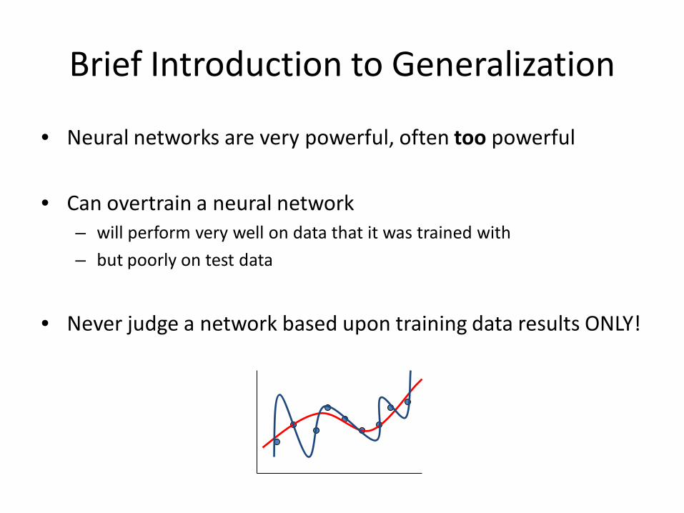
Brief Introduction to Generalization

• Neural networks are very powerful, often too powerful

• Can overtrain a neural network– will perform very well on data that it was trained with– but poorly on test data

• Never judge a network based upon training data results ONLY!

The Learning Curve• We use the Mean Squared Error for training the network

• A plot of Mean Squared Error versus training time (epoch number) is called the learning curve

• Rising learning curve is bad• Oscillating learning curve is usually bad• Decreasing learning curve is good

• MSE is not always the best way to analyze the performance of the network (e.g. classification)

Multiple Datasets

• The most common solution to the “generalization” problem is to divide your data into 3 sets:

– Training data: used to train network

– Cross Validation data: used to actively test the network during training - used to stop training

– Testing data: used to test the network after training

– Production data: desired output is not known (implementation)

•The multi-layer neural network (MNN) is the most commonly used network model for image classification in remote sensing. MNN is usually implemented using the Backpropagation (BP) learning algorithm. The learning process requires a training data set, i.e., a set of training patterns with inputs and corresponding desired outputs. •The essence of learning in MNNs is to find a suitable set of parameters that approximate an unknown input-output relation. Learning in the network is achieved by minimizing the least square differences between the desired and the computed outputs to create an optimal network to best approximate the input-output relation on the restricted domain covered by the training set.

•A typical MNN consists of one input layer, one or more hidden layers and one output layer•MNNs are known to be sensitive to many factors, such as the size and quality of training data set, network architecture, learning rate, overfitting problems

X1

X2

X3

X4

O1

O2

O3

O4

O5

Input Layer

Hidden Layer

Output Layer

•In practical implementations of MNNs, it often happens that a well-trained network with a very low training error fails to classify unseen patterns or produces a low generalization accuracy when applied to a new data set.

•This phenomenon is called overfitting. This is partly because the over-training process makes the network learning focus on specifics of this particular training data which are not the typical characteristics of the whole data set. Thus, it is important to use a cross-validation approach to stop the training at an appropriate time

•Basically, we collect two data sets: training data set and testing data set. During training only the training data set is used to train the network. However, the classification performances with both testing and training data are computed and checked. The training will stop while the training error keeps decreasing and the testing performance starts to deteriorate. This parallel cross-validation approach can ensure that the trained network be an effective classifier to generalize well to new/unseen data and can avoid wasting time to apply an ineffective network to classify other data.

5/23/06 37

NASA Intelligent Systems (IS) ProgramIntelligent Data Understanding (IDU)

Automated Wildfire Detection and Prediction Through

Artificial Neural NetworksJerry Miller (P.I.), NASA, GSFC

Kirk Borne (Co-I), GMUBrian Thomas, University of Maryland

Zhenping Huang, University of Maryland Yuechen Chi, GMU

Donna McNamara, NOAA-NESDIS, Camp Springs, MD George Serafino , NOAA-NESDIS, Camp Springs, MD

38

Short Description of Wildfire Project

• Automated Wildfire Detection (and Prediction)through Artificial Neural Networks (ANN)

– Identify all wildfires in Earth-observing satellite images – Train ANN to mimic human analysts’ classifications– Apply ANN to new data (from 3 remote-sensing

satellites: GOES, AVHRR, MODIS)– Extend NOAA fire product from USA to the whole Earth

39

NOAA’S HAZARD MAPPING SYSTEM

NOAA’s Hazard Mapping System (HMS) is an interactive processing system that allowstrained satellite analysts to manually integrate data from 3 automated fire detectionalgorithms corresponding to the GOES, AVHRR and MODIS sensors. The result is aquality controlled fire product in graphic (Fig 1), ASCII (Table 1) and GIS formats for thecontinental US.

Figure – Hazard Mapping System (HMS) Graphic Fire Product for day 5/19/2003

40

OVERALL TASK OBJECTIVESTo mimic the NOAA-NESDIS Fire Analysts’ subjectivedecision-making and fire detection algorithms with a Neural Network in order to: remove subjectivity in results improve automation & consistency allow NESDIS to expand coverage globally

Sources of subjectivity in Fire Analysts’ decision-making: Fire is not burning very hot, small in areal extent Fire is not burning much hotter than surrounding scene Dependency on Analysts’ “aggressiveness” in finding fires Determination of false detects

41

OLD FORMAT NEW FORMAT (as of May 16, 2003)Lon, Lat Lon, Lat, Time, Satellite, Method of Detection-80.531, 25.351 -80.597, 22.932, 1830, MODIS AQUA, MODIS-81.461, 29.072 -79.648, 34.913, 1829, MODIS, ANALYSIS-83.388, 30.360 -81.048, 33.195, 1829, MODIS, ANALYSIS-95.004, 30.949 -83.037, 36.219, 1829, MODIS, ANALYSIS-93.579, 30.459 -83.037, 36.219, 1829, MODIS, ANALYSIS-108.264, 27.116 -85.767, 49.517, 1805, AVHRR NOAA-16, FIMMA-108.195, 28.151 -84.465, 48.926, 2130, GOES-WEST, ABBA-108.551, 28.413 -84.481, 48.888, 2230, GOES-WEST, ABBA-108.574, 28.441 -84.521, 48.864, 2030, GOES-WEST, ABBA-105.987, 26.549 -84.557, 48.891, 1835, MODIS AQUA, MODIS-106.328, 26.291 -84.561, 48.881, 1655, MODIS TERRA, MODIS-106.762, 26.152 -84.561, 48.881, 1835, MODIS AQUA, MODIS-106.488, 26.006 -89.433, 36.827, 1700, MODIS TERRA, MODIS-106.516, 25.828 -89.750, 36.198, 1845, GOES, ANALYSIS

Hazard Mapping System (HMS) ASCII Fire Product

42

SIMPLIFIED DATA EXTRACTION PROCEDURE

Daily

HMS ASCII

Fire Product

Geographic Coords (lat/lon)

ENVI Function Call

Conversion to Image

Coords (row/col)

Image Ref’s

DATA:

GOES (96 Files/day)

AVHRR (25 Files/day)

MODIS (14 Files/day)

Filter Out

Bad data points

Image

Coords

SpectralData

Neural Network

Training Set

43

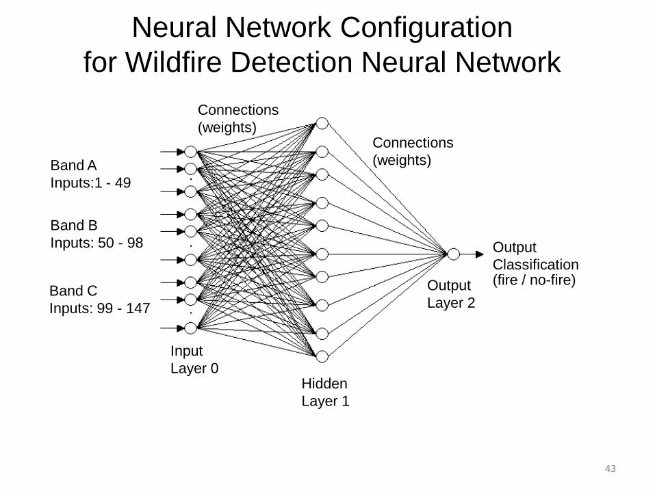
Neural Network Configurationfor Wildfire Detection Neural Network

Connections(weights)

Connections(weights)

InputLayer 0

HiddenLayer 1

OutputLayer 2

OutputClassification

Band AInputs:1 - 49

Band BInputs: 50 - 98

Band CInputs: 99 - 147

(fire / no-fire)

44

Typical Error Matrix(for MODIS instrument)

Fire NonFire Totals

Fire

NonFire

Totals

TRAINING DATA

3007

318(FN)

34213103(TN)

32763152 6428

173(FP)

2834(TP)

True Positive False PositiveFalse Negative True Negative

RESULTS

45

Typical Measures of Accuracy• Overall Accuracy = (TP+TN)/(TP+TN+FP+FN)• Producer’s Accuracy (fire) = TP/(TP+FN)• Producer’s Accuracy (nonfire) = TN/(FP+TN)• User’s Accuracy (fire) = TP/(TP+FP)• User’s Acuracy (nonfire) = TN/(TN+FN)

Accuracy of our NN Classification• Overall Accuracy = 92.4%• Producer’s Accuracy (fire) = 89.9%• Producer’s Accuracy (nonfire) = 94.7%• User’s Accuracy (fire) = 94.2%• User’s Acuracy (nonfire) = 90.7%