Introduction to Multivariate General Linear Models...Types of Multivariate Dependency • Dependency...

Introduction to Multivariate General Linear Models

PSQF 7375 Generalized: Lecture 4 1

• Topics: Taxonomy of multivariate dependency: balanced or unbalanced Multivariate models for balanced outcomes in univariate software 𝑹 matrix choices for residual variance and covariance Fixed effects parameterization choices

3 Parts of Generalized Linear Models

A. Link Function: Transformation of conditional mean to keep predicted outcomes within the bounds of the outcome

B. Same Linear Predictor: How the model linearly predicts the link-transformed conditional mean of the outcome

Btw, I call this as the “model for the means” more generally

C. Conditional Distribution: How the outcome residuals could be distributed given the possible values of the outcome

• Now we need to consider how the model needs to adapt

when residuals are correlated capture “dependency” Btw, I call this as the “model for the variance” more generally

2

B. Same Linear Predictive Model = A. Link

Function C. Actual

Data

PSQF 7375 Generalized: Lecture 4

Types of Multivariate Dependency • Dependency arises whenever multiple outcomes are collected from

the same sampling unit, for example: A single outcome across repeated occasions or under multiple conditions,

or multiple outcomes from the same person (“repeated measures” data) Multiple persons from the same pair (“dyadic” data) Multiple persons from the same group (“clustered” data)

• A key distinction in guiding modeling options is whether the sampling

design is “balanced”—is structured the same for every sampling unit Balanced: all persons have the same potential occasions, conditions,

or outcomes (where potential allows missingness) from a common set Unbalanced: no common set (e.g., observed occasions differ across

persons, number of persons within a group differs across groups)

• We will not cover unbalanced outcomes in this class—they will be covered instead in classes focused on multilevel models (aka, mixed-effects models, hierarchical linear models) involving random intercepts and slopes

3 PSQF 7375 Generalized: Lecture 4

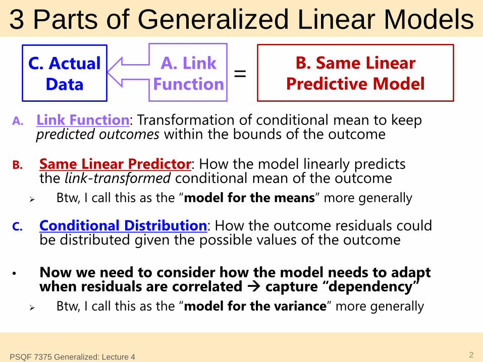
Estimating (Balanced) Multivariate Models • Multivariate models can be estimated by “tricking” univariate software

for general(ized) linear models (e.g., SAS MIXED, STATA MIXED) if each variable is either a predictor OR an outcome, not both, such as when: You want to examine mean differences across the outcomes (e.g., over

time or across conditions, as in traditional Repeated Measures ANOVA) You want to test differences in the effects of predictors

across outcomes (i.e., as in traditional MANOVA) In this case we can build correlations (directly or indirectly)

into the model between outcomes from the same person

• Multivariate models will need to be estimated in “truly” multivariate software (i.e., as path analysis models or structural equation models) if some variables are both predictors and outcomes, such as in mediation e.g., X M Y, in which M is both an outcome of X and a predictor of Y This involves regressions instead of correlations between outcomes

• For both types of analyses we will use likelihood estimation instead of least squares, so that cases with missing outcomes are not removed from the model (for what happens with missing predictors, stay tuned)


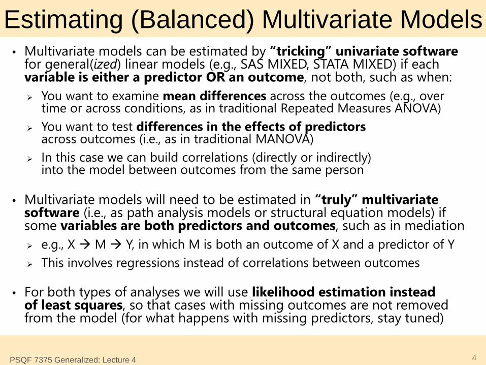
Back to General Linear Models… • Regardless of software, multivariate relations among outcomes

from the same sampling unit can be specified in one of two ways: Directly is only possible for models with normal residuals (GLM)

Linear predictor will only include fixed effects, like usual, because residual dependency is captured directly via residual covariances

Indirectly is the only option using true likelihood estimation for non-normal outcomes (i.e., generalized linear models) Add random intercepts to the linear predictor that capture residual

dependency (so the usual conditional distributions can still be used)

• To understand the difference, we first need to describe models for independent observations using new vocabulary—fun with matrices! Let’s start with this general linear model: 𝒚𝒊 = 𝜷𝟎 + 𝜷𝟏 𝒙𝒊 + 𝒆𝒊

In this “scalar” notation, the assumed independence is hidden… What follows is the “direct” way of including relations among outcomes

(we will see the “indirect” way at work in generalized linear models)


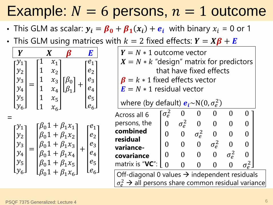
Example: 𝑁 = 6 persons, 𝑛 = 1 outcome • This GLM as scalar: 𝒚𝒊 = 𝜷𝟎 + 𝜷𝟏 𝒙𝒊 + 𝒆𝒊 with binary 𝑥𝑖 = 0 or 1 • This GLM using matrices with 𝑘 = 2 fixed effects: 𝒀 = 𝑿𝜷 + 𝑬

𝑦1𝑦2𝑦3𝑦4𝑦5𝑦6

=

1 𝑥11 𝑥21 𝑥31 𝑥41 𝑥51 𝑥6

𝛽0𝛽1

+

𝑒1𝑒2𝑒3𝑒4𝑒5𝑒6

=

𝑦1𝑦2𝑦3𝑦4𝑦5𝑦6

=

𝛽01 + 𝛽1𝑥1𝛽01 + 𝛽1𝑥2𝛽01 + 𝛽1𝑥3𝛽01 + 𝛽1𝑥4𝛽01 + 𝛽1𝑥5𝛽01 + 𝛽1𝑥6

+

𝑒1𝑒2𝑒3𝑒4𝑒5𝑒6


𝒀 = 𝑁 ∗ 1 outcome vector 𝑿 = 𝑁 ∗ 𝑘 “design” matrix for predictors that have fixed effects 𝜷 = 𝑘 ∗ 1 fixed effects vector 𝑬 = 𝑁 ∗ 1 residual vector

where (by default) 𝒆𝒊~N 0,𝜎𝑒2 Across all 6 persons, the combined residual variance-covariance matrix is “VC”:

𝜎𝑒2 0 0 0 0 00 𝜎𝑒2 0 0 0 00 0 𝜎𝑒2 0 0 00 0 0 𝜎𝑒2 0 00 0 0 0 𝜎𝑒2 00 0 0 0 0 𝜎𝑒2

𝒀 𝑿 𝜷 𝑬

Off-diagonal 0 values independent residuals 𝜎𝑒2 all persons share common residual variance

Review: Univariate Normal PDF

7

( )2

i ii 22

ee

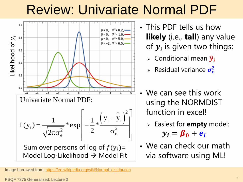
Univariate Normal PDF:

y y1 1f (y ) *exp *22

− = − σπσ

Like

lihoo

d of

• This PDF tells us how likely (i.e., tall) any value of 𝒚𝒊 is given two things: Conditional mean 𝒚�𝒊 Residual variance 𝝈𝒆𝟐

• We can see this work using the NORMDIST function in excel! Easiest for empty model:

𝒚𝒊 = 𝜷𝟎 + 𝒆𝒊 • We can check our math

via software using ML! Sum over persons of log of 𝑓(y𝑖)= Model Log-Likelihood Model Fit

Image borrowed from: https://en.wikipedia.org/wiki/Normal_distribution PSQF 7375 Generalized: Lecture 0

https://en.wikipedia.org/wiki/Normal_distribution

Univariate ML via Excel “NORMDIST”

8

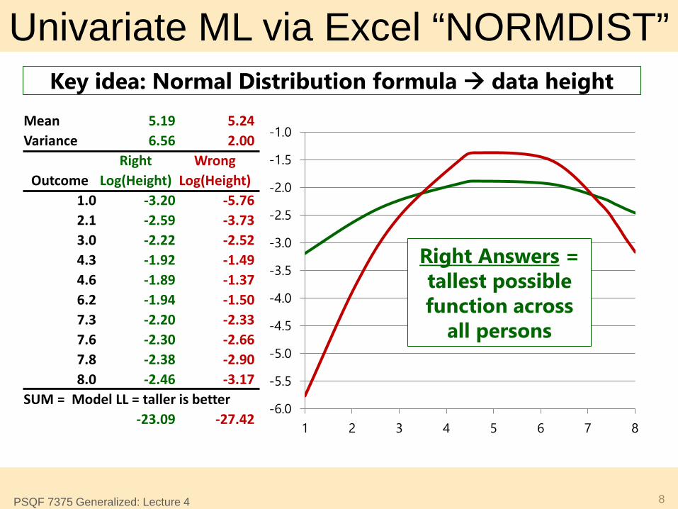
Mean 5.19 5.24 Variance 6.56 2.00

Right Wrong Outcome Log(Height) Log(Height)

1.0 -3.20 -5.76 2.1 -2.59 -3.73 3.0 -2.22 -2.52 4.3 -1.92 -1.49 4.6 -1.89 -1.37 6.2 -1.94 -1.50 7.3 -2.20 -2.33 7.6 -2.30 -2.66 7.8 -2.38 -2.90 8.0 -2.46 -3.17

SUM = Model LL = taller is better -23.09 -27.42

-6.0

-5.5

-5.0

-4.5

-4.0

-3.5

-3.0

-2.5

-2.0

-1.5

-1.0

1 2 3 4 5 6 7 8

Right Answers = tallest possible function across

all persons

Key idea: Normal Distribution formula data height


Review: Conditional Univariate Normal

9

( )2

i ii 22

ee

Univariate Normal PDF:

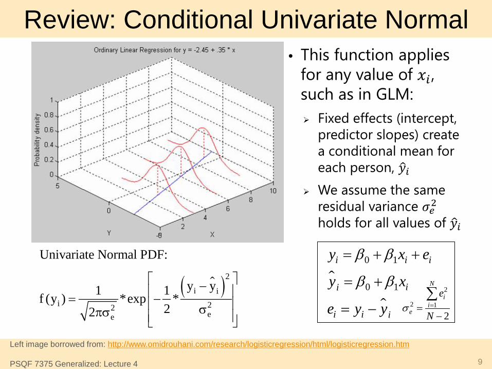
y y1 1f (y ) *exp *22

− = − σπσ

• This function applies for any value of 𝑥𝑖 , such as in GLM: Fixed effects (intercept,

predictor slopes) create a conditional mean for each person, 𝑦�𝑖

We assume the same residual variance 𝜎𝑒2 holds for all values of 𝑦�𝑖

0 1

0 1

= + +

= +

= −

i i i

ii

i i i

y x e

y x

e y y

β β

β β2

2 1

2==−

∑N

ii

e

e

Nσ

Left image borrowed from: http://www.omidrouhani.com/research/logisticregression/html/logisticregression.htm PSQF 7375 Generalized: Lecture 4

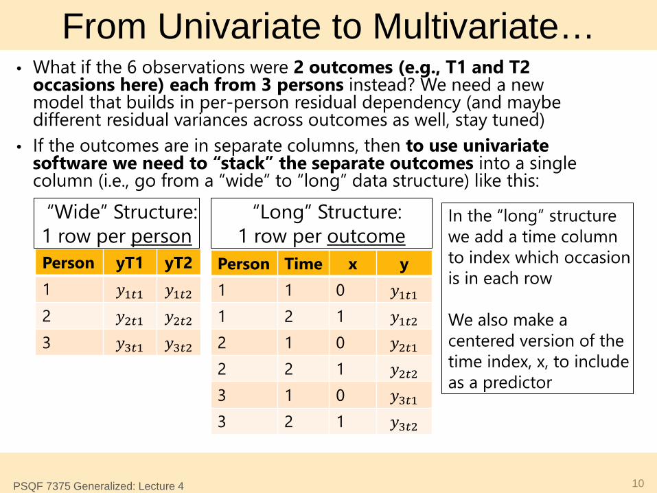
http://www.omidrouhani.com/research/logisticregression/html/logisticregression.htm

From Univariate to Multivariate… • What if the 6 observations were 2 outcomes (e.g., T1 and T2

occasions here) each from 3 persons instead? We need a new model that builds in per-person residual dependency (and maybe different residual variances across outcomes as well, stay tuned)

• If the outcomes are in separate columns, then to use univariate software we need to “stack” the separate outcomes into a single column (i.e., go from a “wide” to “long” data structure) like this:


Person yT1 yT2 1 𝑦1𝑡1 𝑦1𝑡2 2 𝑦2𝑡1 𝑦2𝑡2 3 𝑦3𝑡1 𝑦3𝑡2

Person Time x y 1 1 0 𝑦1𝑡1 1 2 1 𝑦1𝑡2 2 1 0 𝑦2𝑡1 2 2 1 𝑦2𝑡2 3 1 0 𝑦3𝑡1 3 2 1 𝑦3𝑡2

“Wide” Structure: 1 row per person

“Long” Structure: 1 row per outcome

In the “long” structure we add a time column to index which occasion is in each row We also make a centered version of the time index, x, to include as a predictor

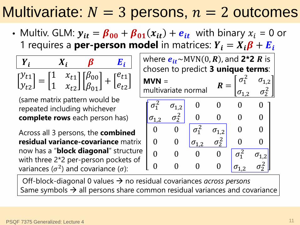
Multivariate: 𝑁 = 3 persons, 𝑛 = 2 outcomes • Multiv. GLM: 𝒚𝒊𝒕 = 𝜷𝟎𝟎 + 𝜷𝟎𝟏 𝒙𝒊𝒕 + 𝒆𝒊𝒕 with binary 𝑥𝑖 = 0 or

1 requires a per-person model in matrices: 𝒀𝒊 = 𝑿𝒊𝜷 + 𝑬𝒊

𝑦𝑡1𝑦𝑡2 = 1 𝑥𝑡1

1 𝑥𝑡2𝛽00𝛽01

+𝑒𝑡1𝑒𝑡2


where 𝒆𝒊𝒕~MVN 0,𝑹 , and 2*2 𝑹 is chosen to predict 3 unique terms:

𝑹 =𝜎12 𝜎1,2

𝜎1,2 𝜎22

(same matrix pattern would be repeated including whichever complete rows each person has) Across all 3 persons, the combined residual variance-covariance matrix now has a “block diagonal” structure with three 2*2 per-person pockets of variances (𝜎2) and covariance (𝜎):

𝒀𝒊 𝑿𝒊 𝜷 𝑬𝒊

Off-block-diagonal 0 values no residual covariances across persons Same symbols all persons share common residual variances and covariance

𝜎12 𝜎1,2 0 0 0 0𝜎1,2 𝜎22 0 0 0 0

0 0 𝜎12 𝜎1,2 0 00 0 𝜎1,2 𝜎22 0 00 0 0 0 𝜎12 𝜎1,2

0 0 0 0 𝜎1,2 𝜎22

MVN = multivariate normal

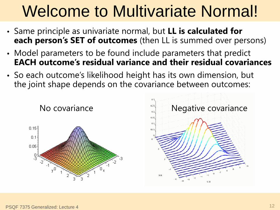
Welcome to Multivariate Normal! • Same principle as univariate normal, but LL is calculated for

each person’s SET of outcomes (then LL is summed over persons) • Model parameters to be found include parameters that predict

EACH outcome’s residual variance and their residual covariances • So each outcome’s likelihood height has its own dimension, but

the joint shape depends on the covariance between outcomes:

12

No covariance Negative covariance


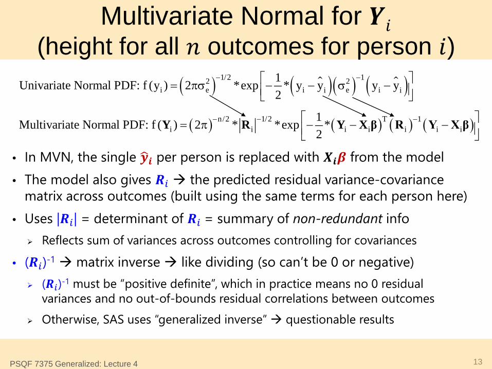
Multivariate Normal for 𝒀𝑖 (height for all 𝑛 outcomes for person 𝑖)

• In MVN, the single 𝒚�𝒊 per person is replaced with 𝑿𝒊𝜷 from the model • The model also gives 𝑹𝑖 the predicted residual variance-covariance

matrix across outcomes (built using the same terms for each person here) • Uses |𝑹𝑖| = determinant of 𝑹𝑖 = summary of non-redundant info

Reflects sum of variances across outcomes controlling for covariances

• (𝑹𝑖)-1 matrix inverse like dividing (so can’t be 0 or negative) (𝑹𝑖)-1 must be “positive definite”, which in practice means no 0 residual

variances and no out-of-bounds residual correlations between outcomes Otherwise, SAS uses “generalized inverse” questionable results

13

( ) ( )( ) ( )

( ) ( ) ( ) ( )

1/2 12 2i e i e ii i

1/2n/2 T 1i i i i i i i

1Univariate Normal PDF: f (y ) 2 *exp * y y y y2

1Multivariate Normal PDF: f ( ) 2 * *exp *2

− −

−− −

= πσ − − σ −

= π − − − Y R Y X β R Y X β


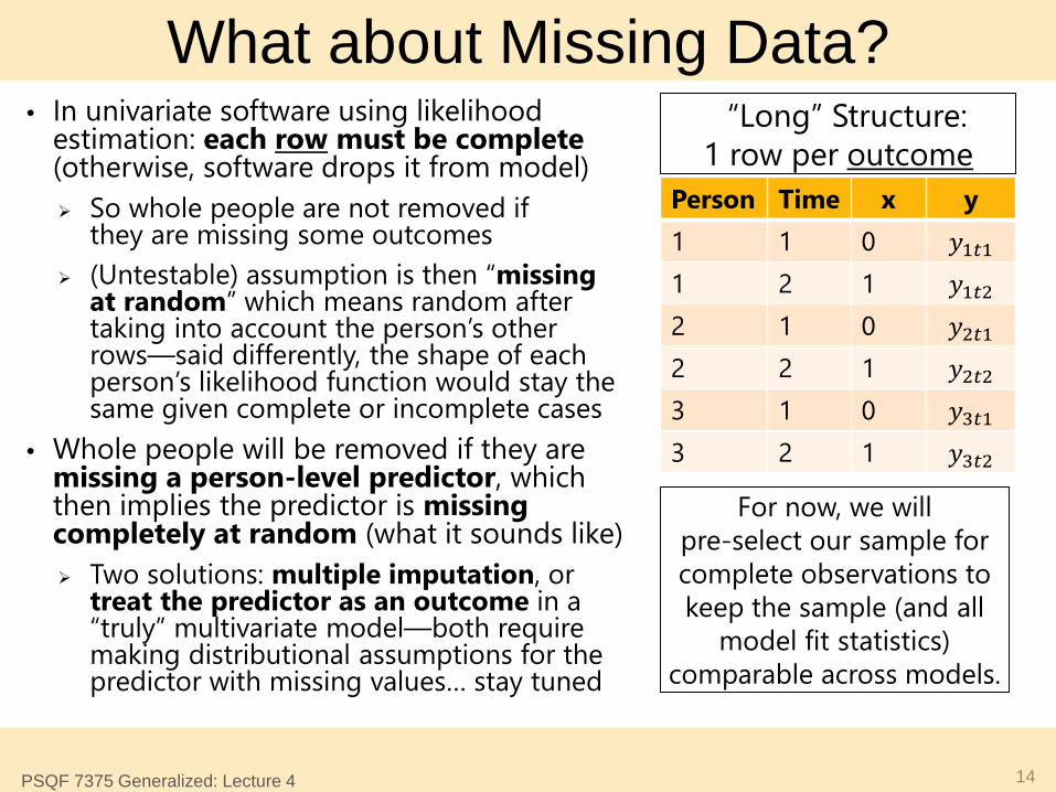
What about Missing Data? • In univariate software using likelihood

estimation: each row must be complete (otherwise, software drops it from model) So whole people are not removed if

they are missing some outcomes (Untestable) assumption is then “missing

at random” which means random after taking into account the person’s other rows—said differently, the shape of each person’s likelihood function would stay the same given complete or incomplete cases

• Whole people will be removed if they are missing a person-level predictor, which then implies the predictor is missing completely at random (what it sounds like) Two solutions: multiple imputation, or

treat the predictor as an outcome in a “truly” multivariate model—both require making distributional assumptions for the predictor with missing values… stay tuned


Person Time x y 1 1 0 𝑦1𝑡1 1 2 1 𝑦1𝑡2 2 1 0 𝑦2𝑡1 2 2 1 𝑦2𝑡2 3 1 0 𝑦3𝑡1 3 2 1 𝑦3𝑡2

“Long” Structure: 1 row per outcome

For now, we will pre-select our sample for complete observations to keep the sample (and all

model fit statistics) comparable across models.

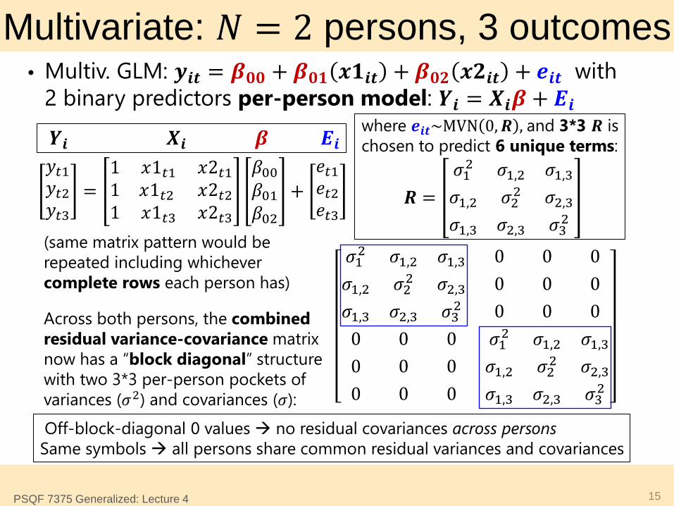
Multivariate: 𝑁 = 2 persons, 3 outcomes • Multiv. GLM: 𝒚𝒊𝒕 = 𝜷𝟎𝟎 + 𝜷𝟎𝟏 𝒙𝟏𝒊𝒕 + 𝜷𝟎𝟐 𝒙𝟐𝒊𝒕 + 𝒆𝒊𝒕 with

2 binary predictors per-person model: 𝒀𝒊 = 𝑿𝒊𝜷 + 𝑬𝒊

𝑦𝑡1𝑦𝑡2𝑦𝑡3

=1 𝑥1𝑡1 𝑥2𝑡11 𝑥1𝑡2 𝑥2𝑡21 𝑥1𝑡3 𝑥2𝑡3

𝛽00𝛽01𝛽02

+𝑒𝑡1𝑒𝑡2𝑒𝑡3


where 𝒆𝒊𝒕~MVN 0,𝑹 , and 3*3 𝑹 is chosen to predict 6 unique terms:

𝑹 =𝜎12 𝜎1,2 𝜎1,3

𝜎1,2 𝜎22 𝜎2,3

𝜎1,3 𝜎2,3 𝜎32

(same matrix pattern would be repeated including whichever complete rows each person has) Across both persons, the combined residual variance-covariance matrix now has a “block diagonal” structure with two 3*3 per-person pockets of variances (𝜎2) and covariances (𝜎):

𝒀𝒊 𝑿𝒊 𝜷 𝑬𝒊

Off-block-diagonal 0 values no residual covariances across persons Same symbols all persons share common residual variances and covariances

𝜎12 𝜎1,2 𝜎1,3 0 0 0𝜎1,2 𝜎22 𝜎2,3 0 0 0𝜎1,3 𝜎2,3 𝜎32 0 0 0

0 0 0 𝜎12 𝜎1,2 𝜎1,3

0 0 0 𝜎1,2 𝜎22 𝜎2,3

0 0 0 𝜎1,3 𝜎2,3 𝜎32

What should the 𝑹 Matrix Look Like? • Goal: predict all unique variances and covariances in 𝑹

The “direct” way of doing so uses only different 𝑹 patterns (“R-side” models, as opposed to “G-side” models, stay tuned)

• Next are 3 “direct” choices for unordered multiple outcomes

(btw, there are more choices for outcomes ordered in time or space) SAS MIXED: REPEATED DVindex /TYPE=?? SUBJECT=PersonID R RCORR; SAS GLIMMIX: RANDOM DVindex /TYPE=?? SUBJECT=PersonID RESIDUAL; Stata MIXED: Goes into option residuals(??, t(DVindex))

Not possible in STATA GLM or MEGLM (as far as I know)

• The 3 choices for 𝑹 patterns we will use differ in 2 respects: Is residual variance (𝜎2) the same across outcomes?

If so, then are residual covariances (𝜎) are also the same across outcome pairs (remember: covariance is unstandardized correlation)

If not, might residual correlations (𝑟) still be the same across outcome pairs (because covariances will differ if variances differ)


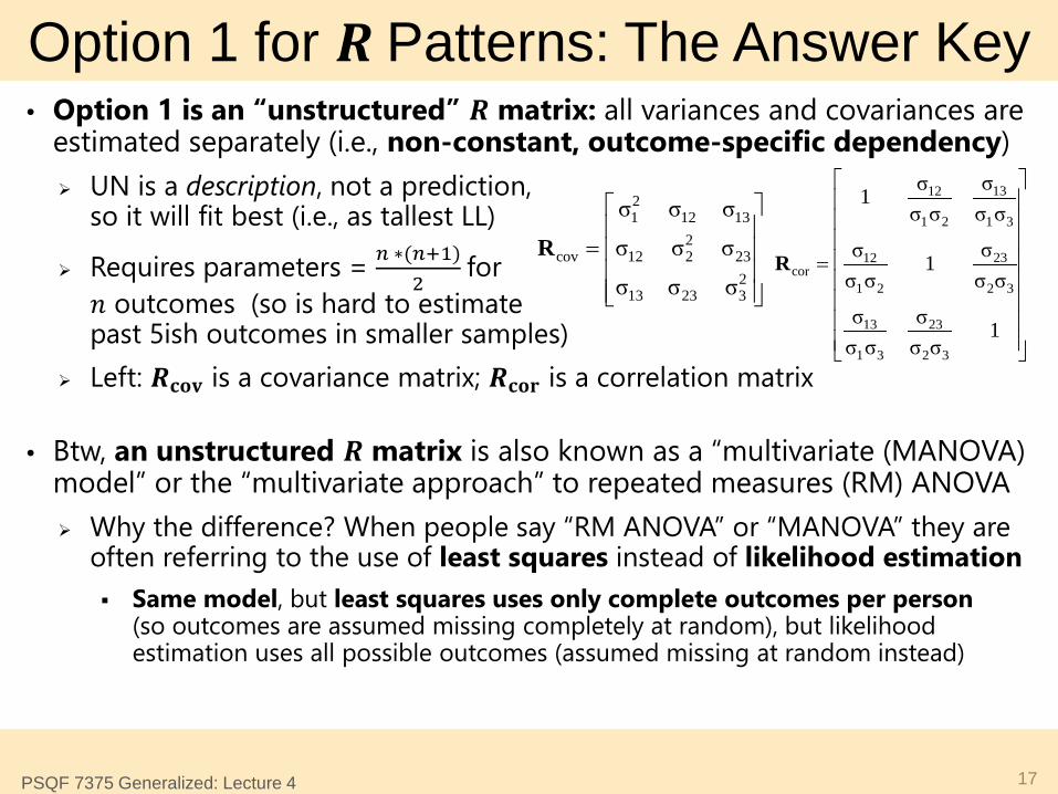
Option 1 for 𝑹 Patterns: The Answer Key • Option 1 is an “unstructured” 𝑹 matrix: all variances and covariances are

estimated separately (i.e., non-constant, outcome-specific dependency) UN is a description, not a prediction,

so it will fit best (i.e., as tallest LL)

Requires parameters = 𝑛 ∗(𝑛+1)2

for 𝑛 outcomes (so is hard to estimate past 5ish outcomes in smaller samples)

Left: 𝑹𝐜𝐜𝐜 is a covariance matrix; 𝑹𝐜𝐜𝐜 is a correlation matrix

• Btw, an unstructured 𝑹 matrix is also known as a “multivariate (MANOVA) model” or the “multivariate approach” to repeated measures (RM) ANOVA Why the difference? When people say “RM ANOVA” or “MANOVA” they are

often referring to the use of least squares instead of likelihood estimation Same model, but least squares uses only complete outcomes per person

(so outcomes are assumed missing completely at random), but likelihood estimation uses all possible outcomes (assumed missing at random instead)


21 12 13

2cov 12 2 23

213 23 3

σ σ σ

σ σ σ

σ σ σ

=

R

1312

1 2 1 3

2312cor

1 2 2 3

13 23

1 3 2 3

σσ1σ σ σ σ

σσ 1σ σ σ σ

σ σ 1σ σ σ σ

=

R

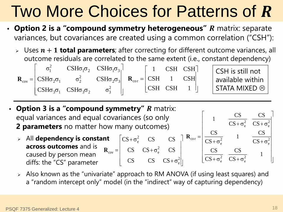
Two More Choices for Patterns of 𝑹 • Option 2 is a “compound symmetry heterogeneous” 𝑹 matrix: separate

variances, but covariances are created using a common correlation (“CSH”): Uses 𝒏 + 𝟏 total parameters; after correcting for different outcome variances, all

outcome residuals are correlated to the same extent (i.e., constant dependency)


21 1 2 1 3

2cov 2 1 2 2 3

23 1 3 2 3

σ CSH CSH

CSH σ CSH

CSH CSH σ

σ σ σ σ

= σ σ σ σ σ σ σ σ

R co r

1 CSH CSHCSH 1 CSHCSH CSH 1

=

R

• Option 3 is a “compound symmetry” 𝑹 matrix: equal variances and equal covariances (so only 2 parameters no matter how many outcomes) All dependency is constant

across outcomes and is caused by person mean diffs: the “CS” parameter

Also known as the “univariate” approach to RM ANOVA (if using least squares) and a “random intercept only” model (in the “indirect” way of capturing dependency)

2 2e e

co r 2 2e e

2 2e e

CS CS1CS CS

CS CS1CS CS

CS CS 1CS CS

+ σ +σ

= + σ +σ

+ σ +σ

R2e

2cov e

2e

CS CS CS

CS CS CS

CS CS CS

+ σ

= + σ + σ

R

CSH is still not available within STATA MIXED

How to Choose among 𝑹 Matrices • Use likelihood ratio tests (LRT): treat difference in −2LL as regular 𝜒2

with DF = # parameters different (also, smallest AIC and BIC win) VC (equal variances, no covariances) is the default and is nested in all others

CS fit better than VC? There’s covariance (dependency) across outcomes CS is nested in CSH, which are both nested in UN (= the data)

CSH fit better than CS? Then variances need to differ by outcome UN fit better than CSH? Then correlations need to differ across outcome pairs

• Goal: find a simpler model that fits not worse than UN UN will always fit best by −2LL because it is trying to recreate

the complete data results (assuming missing at random) Why not just use UN always? If may not always be estimable,

and using a simpler model that fits not worse can lead to greater power (because more unnecessary parameters less power)

• Btw, 𝑹 matrix residual variances and covariances can also be allowed to differ across groups (see example 4a); test if that helps with LRTs

• And in univariate models, residual variance can differ by predictors, too!


Assessing Relative Model Fit, In General • Model for the Means (linear predictor of fixed effects)

which fixed effects of predictors are included in the model Because fixed effects of predictors are unbounded, you can always use

univariate or multivariate Wald tests to see if they contribute to the model (with denominator DF depending on software availability)

Could use LRTs, but only for models estimated with maximum likelihood (not residual maximum likelihood, a better choice for normal residuals)

• Model for the Variance what the pattern of variance and covariance of residuals from the same sampling unit should be DOES require assessment of relative model fit using LRTs: Because

variances cannot be negative, you cannot use Wald test p-values (i.e., that show up in MIXED output next to the variance estimate)

Conditional distributions can only be compared using LRTs (usually with a mixture 𝜒2) or information criteria (AIC, BIC) if they are nested e.g., Poisson and Negative Binomial differ by “stretchy 𝑘”; binomial and

beta-binomial differ by “stretchy 𝜙”; zero-inflation models add an intercept in another submodel that predicts the logit of being an extra 0


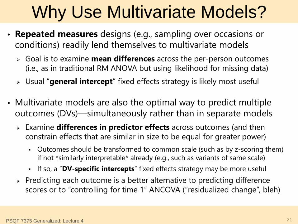
Why Use Multivariate Models? • Repeated measures designs (e.g., sampling over occasions or

conditions) readily lend themselves to multivariate models Goal is to examine mean differences across the per-person outcomes

(i.e., as in traditional RM ANOVA but using likelihood for missing data) Usual “general intercept” fixed effects strategy is likely most useful

• Multivariate models are also the optimal way to predict multiple outcomes (DVs)—simultaneously rather than in separate models Examine differences in predictor effects across outcomes (and then

constrain effects that are similar in size to be equal for greater power) Outcomes should be transformed to common scale (such as by z-scoring them)

if not *similarly interpretable* already (e.g., such as variants of same scale) If so, a “DV-specific intercepts” fixed effects strategy may be more useful

Predicting each outcome is a better alternative to predicting difference scores or to “controlling for time 1” ANCOVA (“residualized change”, bleh)


Differences in Effect Size across DVs

Absolute Value of Effect Size

0

p = .05

Significant for DV A? Yes

Significant for DV B? Yes

Difference in effect size between DV A and DV B?

Scenario 1: Fixed effect is significant for both DVs:

Just because a predictor is significant for both DVs does not mean it has the same magnitude of relationship across DVs!


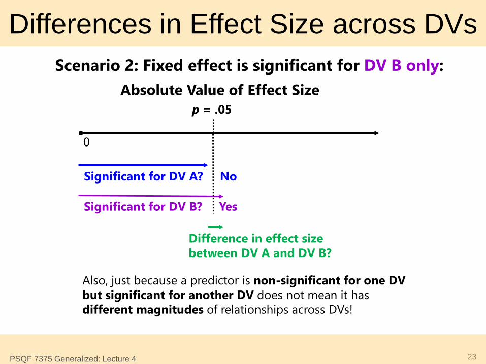
Differences in Effect Size across DVs

Absolute Value of Effect Size

0

Significant for DV A? No

Significant for DV B? Yes

Difference in effect size between DV A and DV B?

Scenario 2: Fixed effect is significant for DV B only:

p = .05

Also, just because a predictor is non-significant for one DV but significant for another DV does not mean it has different magnitudes of relationships across DVs!


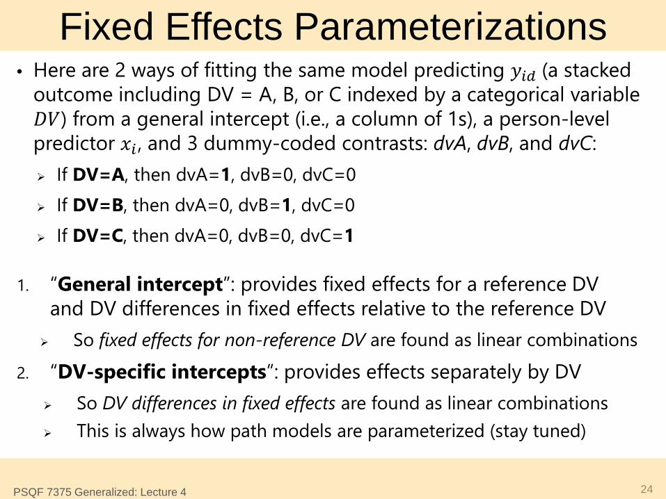
Fixed Effects Parameterizations • Here are 2 ways of fitting the same model predicting 𝑦𝑖𝑖 (a stacked

outcome including DV = A, B, or C indexed by a categorical variable 𝐷𝐷) from a general intercept (i.e., a column of 1s), a person-level predictor 𝑥𝑖 , and 3 dummy-coded contrasts: dvA, dvB, and dvC: If DV=A, then dvA=1, dvB=0, dvC=0 If DV=B, then dvA=0, dvB=1, dvC=0 If DV=C, then dvA=0, dvB=0, dvC=1

1. “General intercept”: provides fixed effects for a reference DV and DV differences in fixed effects relative to the reference DV

So fixed effects for non-reference DV are found as linear combinations 2. “DV-specific intercepts”: provides effects separately by DV

So DV differences in fixed effects are found as linear combinations This is always how path models are parameterized (stay tuned)


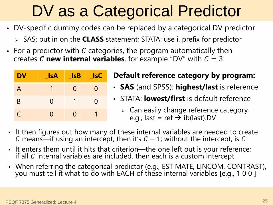
DV as a Categorical Predictor • DV-specific dummy codes can be replaced by a categorical DV predictor

SAS: put in on the CLASS statement; STATA: use i. prefix for predictor • For a predictor with 𝐶 categories, the program automatically then

creates 𝑪 new internal variables, for example “DV” with 𝐶 = 3:


DV _IsA _IsB _IsC

A 1 0 0

B 0 1 0

C 0 0 1

• It then figures out how many of these internal variables are needed to create 𝐶 means—if using an intercept, then it’s 𝐶 − 1; without the intercept, is 𝐶

• It enters them until it hits that criterion—the one left out is your reference; if all 𝐶 internal variables are included, then each is a custom intercept

• When referring the categorical predictor (e.g., ESTIMATE, LINCOM, CONTRAST), you must tell it what to do with EACH of these internal variables [e.g., 1 0 0 ]

Default reference category by program: • SAS (and SPSS): highest/last is reference • STATA: lowest/first is default reference

Can easily change reference category, e.g., last = ref ib(last).DV

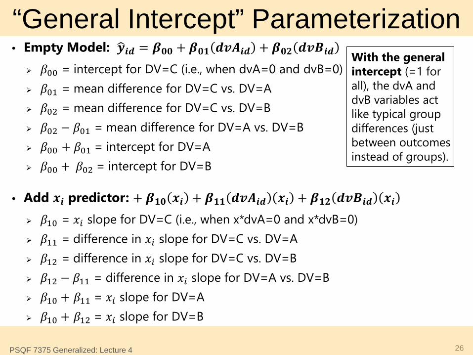
“General Intercept” Parameterization • Empty Model: 𝒚�𝒊𝒅 = 𝜷𝟎𝟎 + 𝜷𝟎𝟏 𝒅𝒅𝑨𝒊𝒅 + 𝜷𝟎𝟐 𝒅𝒅𝑩𝒊𝒅

𝛽00 = intercept for DV=C (i.e., when dvA=0 and dvB=0) 𝛽01 = mean difference for DV=C vs. DV=A 𝛽02 = mean difference for DV=C vs. DV=B 𝛽02 − 𝛽01 = mean difference for DV=A vs. DV=B 𝛽00 + 𝛽01 = intercept for DV=A 𝛽00 + 𝛽02 = intercept for DV=B

• Add 𝒙𝒊 predictor: + 𝜷𝟏𝟎 𝒙𝒊 + 𝜷𝟏𝟏 𝒅𝒅𝑨𝒊𝒅 𝒙𝒊 + 𝜷𝟏𝟐 𝒅𝒅𝑩𝒊𝒅 𝒙𝒊 𝛽10 = 𝑥𝑖 slope for DV=C (i.e., when x*dvA=0 and x*dvB=0) 𝛽11 = difference in 𝑥𝑖 slope for DV=C vs. DV=A 𝛽12 = difference in 𝑥𝑖 slope for DV=C vs. DV=B 𝛽12 − 𝛽11 = difference in 𝑥𝑖 slope for DV=A vs. DV=B 𝛽10 + 𝛽11 = 𝑥𝑖 slope for DV=A 𝛽10 + 𝛽12 = 𝑥𝑖 slope for DV=B


With the general intercept (=1 for all), the dvA and dvB variables act like typical group differences (just between outcomes instead of groups).

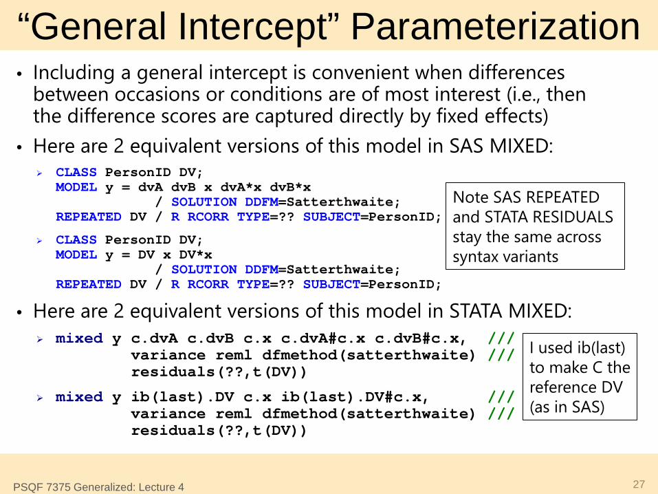
“General Intercept” Parameterization • Including a general intercept is convenient when differences

between occasions or conditions are of most interest (i.e., then the difference scores are captured directly by fixed effects)

• Here are 2 equivalent versions of this model in SAS MIXED: CLASS PersonID DV;

MODEL y = dvA dvB x dvA*x dvB*x / SOLUTION DDFM=Satterthwaite; REPEATED DV / R RCORR TYPE=?? SUBJECT=PersonID;

CLASS PersonID DV; MODEL y = DV x DV*x / SOLUTION DDFM=Satterthwaite; REPEATED DV / R RCORR TYPE=?? SUBJECT=PersonID;

• Here are 2 equivalent versions of this model in STATA MIXED: mixed y c.dvA c.dvB c.x c.dvA#c.x c.dvB#c.x, ///

variance reml dfmethod(satterthwaite) /// residuals(??,t(DV))

mixed y ib(last).DV c.x ib(last).DV#c.x, /// variance reml dfmethod(satterthwaite) /// residuals(??,t(DV))


Note SAS REPEATED and STATA RESIDUALS stay the same across syntax variants

I used ib(last) to make C the reference DV (as in SAS)

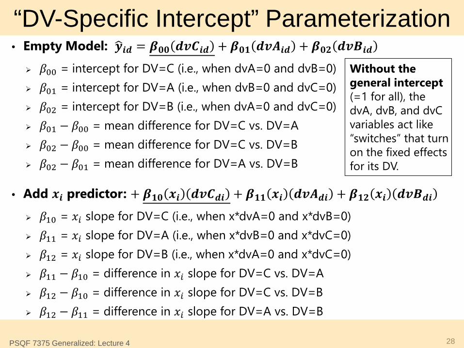
“DV-Specific Intercept” Parameterization • Empty Model: 𝒚�𝒊𝒅 = 𝜷𝟎𝟎 𝒅𝒅𝑪𝒊𝒅 + 𝜷𝟎𝟏 𝒅𝒅𝑨𝒊𝒅 + 𝜷𝟎𝟐 𝒅𝒅𝑩𝒊𝒅

𝛽00 = intercept for DV=C (i.e., when dvA=0 and dvB=0) 𝛽01 = intercept for DV=A (i.e., when dvB=0 and dvC=0) 𝛽02 = intercept for DV=B (i.e., when dvA=0 and dvC=0) 𝛽01 − 𝛽00 = mean difference for DV=C vs. DV=A 𝛽02 − 𝛽00 = mean difference for DV=C vs. DV=B 𝛽02 − 𝛽01 = mean difference for DV=A vs. DV=B

• Add 𝒙𝒊 predictor: + 𝜷𝟏𝟎 𝒙𝒊 𝒅𝒅𝑪𝒅𝒊 + 𝜷𝟏𝟏 𝒙𝒊 𝒅𝒅𝑨𝒅𝒊 + 𝜷𝟏𝟐 𝒙𝒊 𝒅𝒅𝑩𝒅𝒊 𝛽10 = 𝑥𝑖 slope for DV=C (i.e., when x*dvA=0 and x*dvB=0) 𝛽11 = 𝑥𝑖 slope for DV=A (i.e., when x*dvB=0 and x*dvC=0) 𝛽12 = 𝑥𝑖 slope for DV=B (i.e., when x*dvA=0 and x*dvC=0) 𝛽11 − 𝛽10 = difference in 𝑥𝑖 slope for DV=C vs. DV=A 𝛽12 − 𝛽10 = difference in 𝑥𝑖 slope for DV=C vs. DV=B 𝛽12 − 𝛽11 = difference in 𝑥𝑖 slope for DV=A vs. DV=B


Without the general intercept (=1 for all), the dvA, dvB, and dvC variables act like “switches” that turn on the fixed effects for its DV.

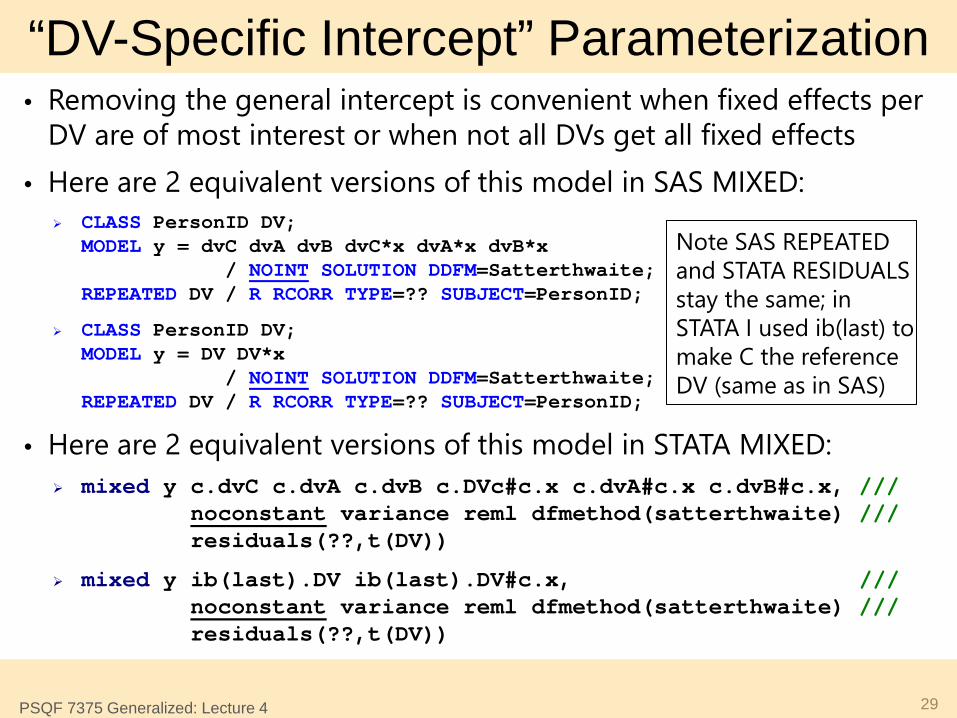
“DV-Specific Intercept” Parameterization • Removing the general intercept is convenient when fixed effects per

DV are of most interest or when not all DVs get all fixed effects • Here are 2 equivalent versions of this model in SAS MIXED:

CLASS PersonID DV; MODEL y = dvC dvA dvB dvC*x dvA*x dvB*x / NOINT SOLUTION DDFM=Satterthwaite; REPEATED DV / R RCORR TYPE=?? SUBJECT=PersonID;

CLASS PersonID DV; MODEL y = DV DV*x / NOINT SOLUTION DDFM=Satterthwaite; REPEATED DV / R RCORR TYPE=?? SUBJECT=PersonID;

• Here are 2 equivalent versions of this model in STATA MIXED: mixed y c.dvC c.dvA c.dvB c.DVc#c.x c.dvA#c.x c.dvB#c.x, ///

noconstant variance reml dfmethod(satterthwaite) /// residuals(??,t(DV))

mixed y ib(last).DV ib(last).DV#c.x, /// noconstant variance reml dfmethod(satterthwaite) /// residuals(??,t(DV))


Note SAS REPEATED and STATA RESIDUALS stay the same; in STATA I used ib(last) to make C the reference DV (same as in SAS)

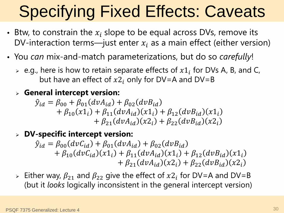
Specifying Fixed Effects: Caveats • Btw, to constrain the 𝑥𝑖 slope to be equal across DVs, remove its

DV-interaction terms—just enter 𝑥𝑖 as a main effect (either version) • You can mix-and-match parameterizations, but do so carefully!

e.g., here is how to retain separate effects of 𝑥1𝑖 for DVs A, B, and C, but have an effect of 𝑥2𝑖 only for DV=A and DV=B

General intercept version: 𝑦�𝑖𝑖 = 𝛽00 + 𝛽01 𝑑𝑑𝐴𝑖𝑖 + 𝛽02 𝑑𝑑𝐵𝑖𝑖 + 𝛽10 𝑥1𝑖 + 𝛽11 𝑑𝑑𝐴𝑖𝑖 𝑥1𝑖 + 𝛽12 𝑑𝑑𝐵𝑖𝑖 𝑥1𝑖 + 𝛽21 𝑑𝑑𝐴𝑖𝑖 𝑥2𝑖 + 𝛽22 𝑑𝑑𝐵𝑖𝑖 𝑥2𝑖

DV-specific intercept version: 𝑦�𝑖𝑖 = 𝛽00 𝑑𝑑𝐶𝑖𝑖 + 𝛽01 𝑑𝑑𝐴𝑖𝑖 + 𝛽02 𝑑𝑑𝐵𝑖𝑖 + 𝛽10 𝑑𝑑𝐶𝑖𝑖 𝑥1𝑖 + 𝛽11 𝑑𝑑𝐴𝑖𝑖 𝑥1𝑖 + 𝛽12 𝑑𝑑𝐵𝑖𝑖 𝑥1𝑖 + 𝛽21 𝑑𝑑𝐴𝑖𝑖 𝑥2𝑖 + 𝛽22 𝑑𝑑𝐵𝑖𝑖 𝑥2𝑖

Either way, 𝛽21 and 𝛽22 give the effect of 𝑥2𝑖 for DV=A and DV=B (but it looks logically inconsistent in the general intercept version)


Wrapping Up… • So far the generalized linear models we have examined have been

univariate models—their LLs assume persons are independent

• But analyzing data in which each sampling unit has more than one outcome requires multivariate models instead We need to add model terms that capture dependency, this semester

for balanced designs (i.e., all persons have the same potential outcomes) For plausibly normal outcomes, dependency can be modeled directly:

we can allow same or different residual variances and covariances across outcomes (in a person-specific R matrix of type UN, CSH, or CS)

We have to use likelihood ratio tests (−2ΔLL as 𝜒2) to compare nested models to decide which fits least worse to protect our fixed effect SEs

• For convenience, fixed effects can be specified in 2 different ways Single general intercept DV terms reflect DV differences Multiple DV-specific intercepts DV terms are switches for own effects


Introduction to Multivariate General Linear Models...Types of Multivariate Dependency • Dependency...

Documents

Transcript of Introduction to Multivariate General Linear Models...Types of Multivariate Dependency • Dependency...