Image Processing and Data Visualization with MATLAB

Hansrudi Noser

June 28-29, 2010

UZH, Multimedia and Robotics Summer School

Introduction to MATLAB(based on MATLAB Help)

Contents

• Overview of MATLAB System

• Matrices and Arrays

• Programming

• Report Generation

Overview: What is MATLAB?

• MATLAB® is a high-performance language for technical computing

• It integrates computation, visualization, and programming in an easy-to-use environment

• Problems and solutions are expressed in familiar mathematical notation.

Overview: Use of MATLAB

• Math and computation• Algorithm development• Data acquisition• Modeling, simulation, and prototyping• Data analysis, exploration, and visualization• Scientific and engineering graphics• Application development, including graphical

user interface building

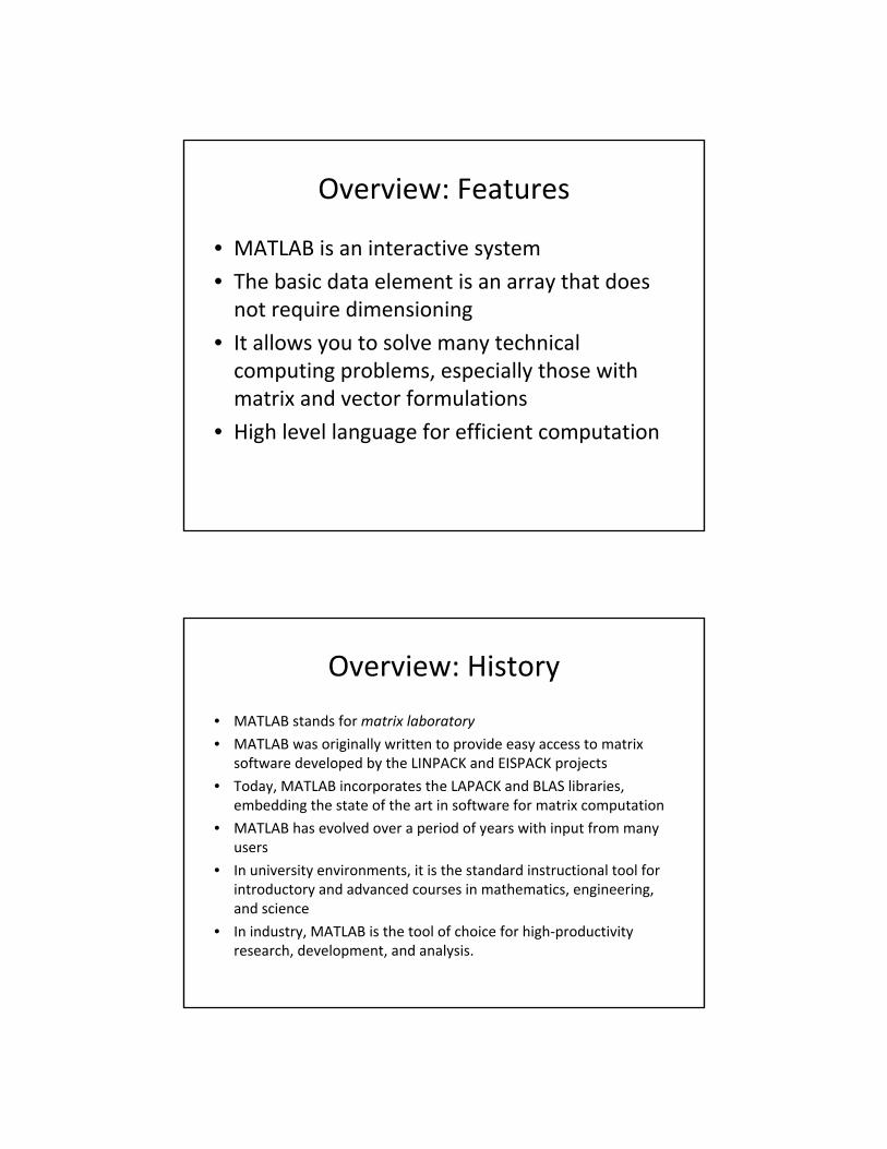
Overview: Features

• MATLAB is an interactive system

• The basic data element is an array that does not require dimensioning

• It allows you to solve many technical computing problems, especially those with matrix and vector formulations

• High level language for efficient computation

Overview: History

• MATLAB stands for matrix laboratory

• MATLAB was originally written to provide easy access to matrix software developed by the LINPACK and EISPACK projects

• Today, MATLAB incorporates the LAPACK and BLAS libraries, embedding the state of the art in software for matrix computation

• MATLAB has evolved over a period of years with input from many users

• In university environments, it is the standard instructional tool for introductory and advanced courses in mathematics, engineering, and science

• In industry, MATLAB is the tool of choice for high-productivity research, development, and analysis.

Overview: Toolboxes

• MATLAB features a family of add-on application-specific solutions called toolboxes.

• Toolboxes allow you to learn and applyspecialized technology.

• Toolboxes are comprehensive collections of MATLAB functions that extend the MATLAB environment to solve particular classes of problems.

• You can add on toolboxes for signal processing, control systems, neural networks, fuzzy logic, wavelets, simulation, and many other areas.

Toolboxes 1

• Math and Optimization– Optimization – Symbolic Math– Partial Differential Equation– Global Optimization

• Statistics and Data Analysis– Statistics– Neural Network– Curve Fitting– Spline– Model-Based Calibration

Toolboxes 2

• Control System Design and Analysis– Control System– System Identification– Fuzzy Logic– Robust Control– Model Predictive Control– Aerospace

• Signal Processing and Communications– Signal Processing– Communications– Filter Design– Wavelet– Fixed-Point– RF

Toolboxes 3

• Image and Video Processing– Image Processing– Video and Image Processing Blockset– Image Acquisition– Mapping

• Test and Measurement– Data Acquisition– Instrument Control– Image Acquisition– System Test– OPC– Vehicle Network

Toolboxes 4

• Computational Biology– Bioinformatics– SimBiology

• Computational Finance– Financial– Financial Derivatives– Datafeed– Fixed-Income– Econometrics

Toolboxes 5

• Application Deployment– MATLAB Compiler– Spreadsheet Link Ex (MS Excel)

• Application Deployment Targets– MATLAB Builder EX (MS Excel)– MATLAB Builder NE (MS .NET Framework)– MATLAB Builder JA (Java)

• Database Connectivity and Reporting– Database Toolbox– MATLAB Report Generator

Simulink Product Family

• Simulink® is an environment for multidomain simulation and Model-Based Design for dynamic and embedded systems

• It provides an interactive graphical environment and a customizable set of block libraries that let you design, simulate, implement, and test a variety of time-varying systems

• It includes communications, controls, signal processing, video processing, and image processing.

• Is not treated in this course• http://www.mathworks.com/products/simulink/

The MATLAB System consists of

• Desktop Tools and Development Environment– Set of tools and facilities that help you use and become more

productive with MATLAB functions and files– Graphical user interfaces for

• MATLAB desktop and Command Window• an editor and debugger• a code analyzer• browsers for viewing help, the workspace, and folders

• Mathematical Function Library– vast collection of computational algorithms ranging from

elementary functions, like sum, sine, cosine, and complex arithmetic, to more sophisticated functions like matrix inverse,matrix eigenvalues, Bessel functions, and fast Fourier transforms.

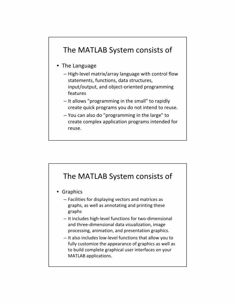
The MATLAB System consists of

• The Language– High-level matrix/array language with control flow

statements, functions, data structures, input/output, and object-oriented programming features

– It allows "programming in the small" to rapidly create quick programs you do not intend to reuse.

– You can also do "programming in the large" to create complex application programs intended for reuse.

The MATLAB System consists of

• Graphics– Facilities for displaying vectors and matrices as

graphs, as well as annotating and printing these graphs

– It includes high-level functions for two-dimensional and three-dimensional data visualization, image processing, animation, and presentation graphics.

– It also includes low-level functions that allow you to fully customize the appearance of graphics as well as to build complete graphical user interfaces on your MATLAB applications.

The MATLAB System consists of

• External Interfaces– The external interfaces library allows you to write

C and Fortran programs that interact with MATLAB.

– It includes facilities for calling routines from MATLAB (dynamic linking), for calling MATLAB as a computational engine, and for reading and writing MAT-files.

Documentation

• The MATLAB program provides extensive documentation, in both printable and HTML format, to help you learn about and use all of its features

• Help menu for– Getting Started– User guides– Function references– Online (web) documentation– Printable documentation (pdf)– Examples / Demos / Movies

• Excellent Training Services

The Desktop of MATLAB

Contents

• Overview of MATLAB System

• Matrices and Arrays

• Programming

• Report Generation

Matrices

• MATLAB = Matrix laboratory• A matrix is a rectangular array of numbers –

the basic data structure in MATLAB• 1-by-1 matrices are scalars• Matrices with only one row or column are

vectors• The operations in MATLAB are designed to be

as natural as possible• MATLAB allows you to work with entire

matrices quickly and easily• Example of matrix in the Renaissance engraving

Melencolia I by the German artist and amateur mathematician Albrecht Dürer.

Entering Matrices

• Enter an explicit list of elements– A = [16 3 2 13; 5 10 11 8; 9 6 7 12; 4 15 14 1]

• Load matrices from external data files– load magik.dat– Data text file

• lines with numbers, separated by blanks, correspond to rows of matrix

– The file name corresponds to variable name (without .dat extension

• Generate matrices using built-in functions– zeros : all zeros– ones : all ones– rand : Uniformly distributed random elements– randn: Normaly distributed random elements

• Create matrices with your own functions in M-files– Text files containing MATLAB code

Z = zeros(2,4) Z =

0 0 0 00 0 0 0

Z = zeros(2,4) Z =

0 0 0 00 0 0 0

A = 16 3 2 13 5 10 11 8 9 6 7 124 15 14 1

A = 16 3 2 13 5 10 11 8 9 6 7 124 15 14 1

R = randn(4,4) R =0.6353 0.0860 -0.3210 -1.2316 -0.6014 -2.0046 1.2366 1.0556 0.5512 -0.4931 -0.6313 -0.1132-1.0998 0.4620 -2.3252 0.3792

R = randn(4,4) R =0.6353 0.0860 -0.3210 -1.2316 -0.6014 -2.0046 1.2366 1.0556 0.5512 -0.4931 -0.6313 -0.1132-1.0998 0.4620 -2.3252 0.3792

Matrix Operation: sum

• sum(A)– Summation along first index : Result

is row vector

• sum(A,2)– Summation along the second index:

Result is column vector

sum(A)

ans = 34 34 34 34

sum(A)

ans = 34 34 34 34

sum(A,2)

ans =34343434

sum(A,2)

ans =34343434

A =16 3 2 135 10 11 89 6 7 124 15 14 1

A =16 3 2 135 10 11 89 6 7 124 15 14 1

Matrix Operation: transpose

• Two transpose operators: ‘ and .’• ‘ operator (A’)

– complex conjugate transposition. It flips a matrix about its main diagonal, and also changes the sign of the imaginary component of any complex elements of the matrix

• .’ operator (A.’)– transposition without affecting the sign

of complex elements. For matrices containing all real elements, the two operators return the same result

A'ans =

16 5 9 43 10 6 152 11 7 14

13 8 12 1

A'ans =

16 5 9 43 10 6 152 11 7 14

13 8 12 1

B = [1 2 3+3i];

B'ans =

1.0000 2.0000 3.0000 - 3.0000i

B.'ans =

1.0000 2.0000 3.0000 + 3.0000i

B = [1 2 3+3i];

B'ans =

1.0000 2.0000 3.0000 - 3.0000i

B.'ans =

1.0000 2.0000 3.0000 + 3.0000i

A =16 3 2 135 10 11 89 6 7 124 15 14 1

A =16 3 2 135 10 11 89 6 7 124 15 14 1

Matrix Operations: diag, fliplr

• diag(A) returns the main diagonal vector of A

• sum(diag(A)) returns the sum of the diagonal elements of A: the trace of A

• fliplr(A) flips the matrix from left to right

• sum(diag(fliplr(A))) returns the sum of the antidiagonal of A)

• diag(diag(A)) returns a diagonal matrix

diag(A)ans =

161071

diag(A)ans =

161071

sum(diag(A))ans =

34

sum(diag(A))ans =

34

diag(diag(A))ans =

16 0 0 00 10 0 00 0 7 00 0 0 1

diag(diag(A))ans =

16 0 0 00 10 0 00 0 7 00 0 0 1

fliplr(A)ans =

13 2 3 168 11 10 5

12 7 6 91 14 15 4

fliplr(A)ans =

13 2 3 168 11 10 5

12 7 6 91 14 15 4

sum(diag(fliplr(A)))ans =

34

sum(diag(fliplr(A)))ans =

34

A =16 3 2 135 10 11 89 6 7 124 15 14 1

A =16 3 2 135 10 11 89 6 7 124 15 14 1

Subscripts

• The element in row i and column j of A is denoted by A(i,j)

• Numbering starts from 1 not 0!• A single subscript is the usual way

of referencing row and column vectors – However, it can also apply to a fully

two-dimensional matrix, in which case the array is regarded as one long column vector formed from the columns of the original matrix

– So, for the magic square, A(8) is another way of referring to the value 15 stored in A(4,2)

A(1,4) + A(2,4) + A(3,4) + A(4,4)

ans =34

A =16 3 2 135 10 11 89 6 7 124 15 14 1

A =16 3 2 135 10 11 89 6 7 124 15 14 1

1

2

3

84

5

16

A(8)

Subscripts

• The access of an element outside of the matrix produces an error

• Conversely, if you store a value in an element outside of the matrix, its size increases to accommodate the newcomer

t = A(4,5) Index exceeds matrix dimensions.t = A(4,5) Index exceeds matrix dimensions.

A =16 3 2 135 10 11 89 6 7 124 15 14 1

A =16 3 2 135 10 11 89 6 7 124 15 14 1

X = A;X(4,5) = 17

X =16 3 2 13 05 10 11 8 09 6 7 12 04 15 14 1 17

X = A;X(4,5) = 17

X =16 3 2 13 05 10 11 8 09 6 7 12 04 15 14 1 17

The Colon Operator :

• The colon, :, is one of the most important MATLAB operators. It occurs in several different forms

• 1:5– is a row vector containing the

integers from 1 to 5

• 100:-11:50– To obtain nonunit spacing, specify

an increment

• 0:pi/4:pi

c1 = 1:5c1 =

1 2 3 4 5

c1 = 1:5c1 =

1 2 3 4 5

c2 = 100:-11:50c2 =

100 89 78 67 56

c2 = 100:-11:50c2 =

100 89 78 67 56

0:pi/4:pians =

0 0.7854 1.5708 2.3562 3.1416

0:pi/4:pians =

0 0.7854 1.5708 2.3562 3.1416

The Colon Operator

• A(1:k,j)– the first k elements of the jth column of A– For example: sum(A(1:4,4)) computes the sum of

the fourth column

• The colon by itself refers to all the elements in a row or column of a matrix and the keyword end refers to the last row or column– sum(A(:,end)) computes the sum of the elements

in the last column of A

Magic

• Magic is a built-in function that creates magic squares of almost any size

• swap the two middle columns– This subscript indicates that—

for each of the rows of matrix B—reorder the elements in the order 1, 3, 2, 4

B = magic(4)B =

16 2 3 135 11 10 89 7 6 124 14 15 1

B = magic(4)B =

16 2 3 135 11 10 89 7 6 124 14 15 1

A = B(:,[1 3 2 4])

A =

16 3 2 135 10 11 89 6 7 124 15 14 1

A = B(:,[1 3 2 4])

A =

16 3 2 135 10 11 89 6 7 124 15 14 1

Variables in MATLAB

• MATLAB does not require any type declarations or dimension statements

• When MATLAB encounters a new variable name, it automatically creates the variable and allocates the appropriate amount of storage

• If the variable already exists, MATLAB changes its contents and, if necessary, allocates new storage.

Numbers in MATLAB

• MATLAB uses conventional decimal notation, with an optional decimal point and leading plus or minus sign, for numbers

• Scientific notation uses the letter e to specify a power-of-ten scale factor

• Imaginary numbers use either i or j as a suffix– Attention: i or j can be redefined

(i=2)

• Examples 3 -99 0.0001 9.6397238 1.60210e-206.02252e23 1i -3.14159j 3e5i3 -99 0.0001 9.6397238 1.60210e-206.02252e23 1i -3.14159j 3e5i

ians =

0 + 1.0000i

i=2i =

2

ians =

0 + 1.0000i

i=2i =

2

Operators

• Expressions use familiar arithmetic operators and precedence rules.

+ Addition- Subtraction* Multiplication/ Division\ Left division^ Power‘ Complex conjugate transpose( ) Specify evaluation order

+ Addition- Subtraction* Multiplication/ Division\ Left division^ Power‘ Complex conjugate transpose( ) Specify evaluation order

Functions

• MATLAB provides a large number of standard elementary mathematical functions, including abs, sin, cos, sqrt, …

• Several special functions provide values of useful constants

pi 3.14159265...i Imaginary unit, j Same as ieps Floating-point relative precisionrealmin Smallest floating-point numberRealmax Largest floating-point numberInf InfinityNaN Not-a-number

pi 3.14159265...i Imaginary unit, j Same as ieps Floating-point relative precisionrealmin Smallest floating-point numberRealmax Largest floating-point numberInf InfinityNaN Not-a-number

Generating Matrices

• Four functions that generate basic matrices

Z = zeros(2,4)Z =

0 0 0 00 0 0 0

Z = zeros(2,4)Z =

0 0 0 00 0 0 0

F = 5*ones(3,3)F =

5 5 55 5 55 5 5

F = 5*ones(3,3)F =

5 5 55 5 55 5 5

N = fix(10*rand(1,10))N =

8 9 1 9 6 0 2 5 9 9

N = fix(10*rand(1,10))N =

8 9 1 9 6 0 2 5 9 9

R = randn(4,4)R =

-1.3499 0.7147 1.4090 0.71723.0349 -0.2050 1.4172 1.63020.7254 -0.1241 0.6715 0.4889

-0.0631 1.4897 -1.2075 1.0347

R = randn(4,4)R =

-1.3499 0.7147 1.4090 0.71723.0349 -0.2050 1.4172 1.63020.7254 -0.1241 0.6715 0.4889

-0.0631 1.4897 -1.2075 1.0347

Concatenation

• the process of joining small matrices to make bigger ones

A = [16.0 3.0 2.0 13.05.0 10.0 11.0 8.09.0 6.0 7.0 12.04.0 15.0 14.0 1.0 ];

A = [16.0 3.0 2.0 13.05.0 10.0 11.0 8.09.0 6.0 7.0 12.04.0 15.0 14.0 1.0 ];

B = [A A+32; A+48 A+16]B =

16 3 2 13 48 35 34 455 10 11 8 37 42 43 409 6 7 12 41 38 39 444 15 14 1 36 47 46 33

64 51 50 61 32 19 18 2953 58 59 56 21 26 27 2457 54 55 60 25 22 23 2852 63 62 49 20 31 30 17

B = [A A+32; A+48 A+16]B =

16 3 2 13 48 35 34 455 10 11 8 37 42 43 409 6 7 12 41 38 39 444 15 14 1 36 47 46 33

64 51 50 61 32 19 18 2953 58 59 56 21 26 27 2457 54 55 60 25 22 23 2852 63 62 49 20 31 30 17

sum(B)ans =

260 260 260 260 260 260 260 260

sum(B)ans =

260 260 260 260 260 260 260 260

Deleting Row and Columns

• You can delete rows and columns from a matrix using just a pair of square brackets

X = AX =

16 3 2 135 10 11 89 6 7 124 15 14 1

X = AX =

16 3 2 135 10 11 89 6 7 124 15 14 1

X(:,2) = []X =

16 2 135 11 89 7 124 14 1

X(:,2) = []X =

16 2 135 11 89 7 124 14 1

X(1,2) = []??? Subscripted assignment dimension mismatch.X(1,2) = []??? Subscripted assignment dimension mismatch.

X(2:2:10) = []X =

16 9 2 7 13 12 1

X(2:2:10) = []X =

16 9 2 7 13 12 1

Deletes sequence of elements, and reshapes the remaining elements into a row vector.

Deletes second column

Linear Algebra

• Informally, the terms matrix and array are often used interchangeably

• A matrix is a two-dimensional numeric array that represents a linear transformation

• The mathematical operations defined on matrices are the subject of linear algebra

• Addition of two matrices: +

–

– Both matrices must have the same dimensions– Element by element addition– Ex: The addition of a matrix to its transpose

produces a symmetric matrix

A =16 3 2 135 10 11 89 6 7 124 15 14 1

A =16 3 2 135 10 11 89 6 7 124 15 14 1

A + A'ans =

32 8 11 178 20 17 23

11 17 14 2617 23 26 2

A + A'ans =

32 8 11 178 20 17 23

11 17 14 2617 23 26 2

, 1,.., , 1,..ij ij ij

C A Bc a b i m j n

= += + = =

Matrix Multiplication

• The multiplication symbol, *, denotes the matrix multiplication involving inner products between rows and columns

1

, , ,

*

* , 1,..., ; 1,...,p

ij ik kjk

A m pB p nC m nC A B

c a b i m j n=

×××

=

= = =

. . . . . . . . . . . . . . .

. . . . . . . . . . . . * . . . . . . . . . . . . . . .

. . . . . . . . . . . . . . .

. . . . . . . . . . . . . . .

ij ij ijc a b

=

i

j

i

j

Matrix Multiplication: Examples

• Multiplying the transpose of a matrix by the original matrix produces a symmetric matrix

• Matrix multiplication is not commutativ

• Some more examples with vectors

A'*Aans =

378 212 206 360212 370 368 206206 368 370 212360 206 212 378

A'*Aans =

378 212 206 360212 370 368 206206 368 370 212360 206 212 378

A =16 3 2 135 10 11 89 6 7 124 15 14 1

A =16 3 2 135 10 11 89 6 7 124 15 14 1

A*A'ans =

438 236 332 150236 310 278 332332 278 310 236150 332 236 438

A*A'ans =

438 236 332 150236 310 278 332332 278 310 236150 332 236 438

a=[1 2 3]a =

1 2 3

b=[4; 5; 6]b =

456

a=[1 2 3]a =

1 2 3

b=[4; 5; 6]b =

456

a*bans =

32

a*bans =

32

b*aans =

4 8 125 10 156 12 18

b*aans =

4 8 125 10 156 12 18

a'*b??? Error using ==> mtimesInner matrix dimensions must agree.

a'*b??? Error using ==> mtimesInner matrix dimensions must agree.

Arrays

• When they are taken away from the world of linear algebra, matrices become two-dimensional numeric arrays

• Arithmetic operations on arrays are done element by element

• This means that addition and subtraction are the same for arrays and matrices

• However multiplicative operations are different. MATLAB uses a dot, or decimal point, as part of the notation for multiplicative array operations

+ Addition- Subtraction.* Element-by-element mult../ Element-by-element div.\ Element-by-element left div..^ Element-by-element power.’ Unconjugated array transpose

+ Addition- Subtraction.* Element-by-element mult../ Element-by-element div.\ Element-by-element left div..^ Element-by-element power.’ Unconjugated array transpose

A =16 3 2 135 10 11 89 6 7 124 15 14 1

A =16 3 2 135 10 11 89 6 7 124 15 14 1

A.*Aans =

256 9 4 16925 100 121 6481 36 49 14416 225 196 1

A.*Aans =

256 9 4 16925 100 121 6481 36 49 14416 225 196 1

Building Tables

• Array operations are useful for building tables

• The elementary math functions operate on arrays element by element

>> n = (0:9)'n =

0123456789

>> n = (0:9)'n =

0123456789

>> pows = [n n.^2 2.^n]pows =

0 0 11 1 22 4 43 9 84 16 165 25 326 36 647 49 1288 64 2569 81 512

>> pows = [n n.^2 2.^n]pows =

0 0 11 1 22 4 43 9 84 16 165 25 326 36 647 49 1288 64 2569 81 512

format short gx = (1:0.1:2)'x =

11.11.21.31.41.51.61.71.81.9

2

format short gx = (1:0.1:2)'x =

11.11.21.31.41.51.61.71.81.9

2

logs = [x log10(x)]logs =

1 01.1 0.0413931.2 0.0791811.3 0.113941.4 0.146131.5 0.176091.6 0.204121.7 0.230451.8 0.255271.9 0.27875

2 0.30103

logs = [x log10(x)]logs =

1 01.1 0.0413931.2 0.0791811.3 0.113941.4 0.146131.5 0.176091.6 0.204121.7 0.230451.8 0.255271.9 0.27875

2 0.30103

Multivariate Data

• MATLAB uses column-oriented analysis for multivariate statistical data

• Each column in a data set represents a variable and each row an observation

• The (i,j)th element is the ith observation of the jthvariable

>> D = [ 72 134 3.281 201 3.569 156 7.182 148 2.475 170 1.2 ];

>> D = [ 72 134 3.281 201 3.569 156 7.182 148 2.475 170 1.2 ];

>> mu = mean(D), sigma = std(D)mu =

75.8 161.8 3.48sigma =

5.6303 25.499 2.2107

>> mu = mean(D), sigma = std(D)mu =

75.8 161.8 3.48sigma =

5.6303 25.499 2.2107

heart rate / weight / hours of exercise

Mean and standard deviation

Scalar Expansion

• Matrices and scalars can be combined in several different ways. For example, a scalar is subtracted from a matrix by subtracting it from each element

• With scalar expansion, MATLAB assigns a specified scalar to all indices in a range

>> B = A - 8.5B =

7.5 -5.5 -6.5 4.5-3.5 1.5 2.5 -0.50.5 -2.5 -1.5 3.5

-4.5 6.5 5.5 -7.5

>> B = A - 8.5B =

7.5 -5.5 -6.5 4.5-3.5 1.5 2.5 -0.50.5 -2.5 -1.5 3.5

-4.5 6.5 5.5 -7.5

A =16 3 2 135 10 11 89 6 7 124 15 14 1

A =16 3 2 135 10 11 89 6 7 124 15 14 1

>>B(1:2,2:3) = 0B =

7.5 0 0 4.5-3.5 0 0 -0.50.5 -2.5 -1.5 3.5

-4.5 6.5 5.5 -7.5

>>B(1:2,2:3) = 0B =

7.5 0 0 4.5-3.5 0 0 -0.50.5 -2.5 -1.5 3.5

-4.5 6.5 5.5 -7.5

Logical Subscripting

• The logical vectors created from logical and relational operations can be used to reference subarrays

• Suppose X is an ordinary matrix and L is a matrix of the same size that is the result of some logical operation– Then X(L) specifies the elements of X where the elements of L

are nonzero.• Example: Remove the missing observation (marked with

NaN) in a data vector

>> x = [2.1 1.7 1.6 1.5 NaN 1.9 1.8 1.5 5.1 1.8 1.4 2.2 1.6 1.8];

>> L=isfinite(x)L =

1 1 1 1 0 1 1 1 1 1 1 1 1 1

>> x=x(L)x = 2.1 1.7 1.6 1.5 1.9 1.8 1.5 5.1 1.8 1.4 2.2 1.6 1.8

>> x = [2.1 1.7 1.6 1.5 NaN 1.9 1.8 1.5 5.1 1.8 1.4 2.2 1.6 1.8];

>> L=isfinite(x)L =

1 1 1 1 0 1 1 1 1 1 1 1 1 1

>> x=x(L)x = 2.1 1.7 1.6 1.5 1.9 1.8 1.5 5.1 1.8 1.4 2.2 1.6 1.8

Logical Subscripting: Example

• For another example, highlight the location of the prime numbers in Dürer's magic square by using logical indexing and scalar expansion to set the nonprimes to 0

>> A(~isprime(A)) = 0

A =

0 3 2 135 0 11 00 0 7 00 0 0 0

>> A(~isprime(A)) = 0

A =

0 3 2 135 0 11 00 0 7 00 0 0 0

>> isprime(A)

ans =

0 1 1 11 0 1 00 0 1 00 0 0 0

>> isprime(A)

ans =

0 1 1 11 0 1 00 0 1 00 0 0 0

>> ~isprime(A)

ans =

1 0 0 00 1 0 11 1 0 11 1 1 1

>> ~isprime(A)

ans =

1 0 0 00 1 0 11 1 0 11 1 1 1

A =16 3 2 135 10 11 89 6 7 124 15 14 1

A =16 3 2 135 10 11 89 6 7 124 15 14 1

Logical Subscripting: Example 2

• Remove outliers from data vector

>> data = 10*rand(10,1)

data =

1.57619.70599.57174.85388.00281.41894.21769.15747.92219.5949

>> data = 10*rand(10,1)

data =

1.57619.70599.57174.85388.00281.41894.21769.15747.92219.5949

>> L = (data > 1) & (data < 9)

L =

1001111010

>> L = (data > 1) & (data < 9)

L =

1001111010

>> data(L)

ans =

1.57614.85388.00281.41894.21767.9221

>> data(L)

ans =

1.57614.85388.00281.41894.21767.9221

data((data > 1) & (data < 9));data((data > 1) & (data < 9));

The find function

• The find function determines the indices of array elements that meet a given logical condition

• In its simplest form, find returns a column vector of indices– Transpose that vector to obtain a row vector of indices

A =16 3 2 135 10 11 89 6 7 124 15 14 1

A =16 3 2 135 10 11 89 6 7 124 15 14 1

>> k = find(isprime(A))‘

k =

2 5 9 10 11 13

>> k = find(isprime(A))‘

k =

2 5 9 10 11 13

>> A(k)

ans =

5 3 2 11 7 13

>> A(k)

ans =

5 3 2 11 7 13

>> A(k) = NaN

A =

16 NaN NaN NaNNaN 10 NaN 89 6 NaN 124 15 14 1

>> A(k) = NaN

A =

16 NaN NaN NaNNaN 10 NaN 89 6 NaN 124 15 14 1

When you use k as a left-hand-side Index in an assignment statement, the matrix structure is preserved

Application: Circle Fit• Given

– A set of 2D data points lying more or less on a circle

• Problem– Find center and radius of circle which best fits to the

data points (least squares method)

• Solution– Get data

– Develop method for best circle fit of data

– Compute and visualize result

Application: Get Data• Normally, data come

from acquisition, but in our case they are computed

% Generation of data pointst=(0:0.3:pi)'r = rand(size(t,1),1)+10x = r.*cos(t)y = r.*sin(t)plot(x,y,'*')title('Data points','FontSize',16)

% Generation of data pointst=(0:0.3:pi)'r = rand(size(t,1),1)+10x = r.*cos(t)y = r.*sin(t)plot(x,y,'*')title('Data points','FontSize',16)

t =0

0.30000.60000.90001.20001.50001.80002.10002.40002.70003.0000

r =10.296310.744710.189010.686810.183510.368510.625610.780210.081110.929410.7757

x =10.296310.26488.40936.64303.69010.7334

-2.4142-5.4424-7.4338-9.8810

-10.6679

y =0

3.17535.75318.37129.4914

10.342510.34779.30566.80944.67101.5207

( )Parametric circle

cossin( )

0,...,2

tcircle r

tt π

= ⋅

=

Application: Method

( ) ( )22 2

2 2

2 2 2

022

x y

x

x

x x

x c y c r

x y ax by ca cb cc c c r

− + − =

+ + + + == −= −

= + −

2 2

2 2

/ 2/ 2

x

y

x x

ax by c x yc ac b

r c c c

+ + = − −= −= −

= + −

Basic equation of a circleBasic equation of a circle Can be rewritten asCan be rewritten as

( )( )

, 2D data point

, center of circle

radius of circle, , unknown variables

x y

x y

c c

ra b c

( )

2 21 1 1 1

2 22 2 2 2

2 23 3 3 3

2 2

data point i

111

... ... ... ...1

i i

n n n n

x y

Ax bx y x yx y a x yx y b x y

cx y x y

=

− − − − = − − − −

System of equationsSystem of equations

Solve the overdetermined system of equationsin the least squares sense!

\x A b=

Application: Computation of the solutionMATLAB code

% Compute the solutionabc = [x y ones(length(x),1)] \ -(x.^2 + y.^2);a = abc(1); b = abc(2); c = abc(3);cx = -a/2;cy = -b/2;radius = sqrt((cx^2 + cy^2) - c);

% Compute the solutionabc = [x y ones(length(x),1)] \ -(x.^2 + y.^2);a = abc(1); b = abc(2); c = abc(3);cx = -a/2;cy = -b/2;radius = sqrt((cx^2 + cy^2) - c);

>> cxcx =

0.0281

>> cycy =

-0.1915

>> radiusradius =

10.7021

>> cxcx =

0.0281

>> cycy =

-0.1915

>> radiusradius =

10.7021

Result

>>[x y ones(length(x),1)]ans =

10.81 0 1.0010.42 3.22 1.008.36 5.72 1.006.78 8.55 1.003.85 9.91 1.000.71 10.07 1.00

-2.34 10.01 1.00-5.32 9.10 1.00-8.08 7.40 1.00-9.91 4.69 1.00

-10.06 1.43 1.00

>>[x y ones(length(x),1)]ans =

10.81 0 1.0010.42 3.22 1.008.36 5.72 1.006.78 8.55 1.003.85 9.91 1.000.71 10.07 1.00

-2.34 10.01 1.00-5.32 9.10 1.00-8.08 7.40 1.00-9.91 4.69 1.00

-10.06 1.43 1.00

>> -(x.^2 + y.^2)ans =

-116.96-118.94-102.56-119.10-113.05-101.96-105.65-111.24-120.07-120.23-103.18

>> -(x.^2 + y.^2)ans =

-116.96-118.94-102.56-119.10-113.05-101.96-105.65-111.24-120.07-120.23-103.18

>>abc =-0.05620.3830

-114.4976

>>abc =-0.05620.3830

-114.4976

Intermediate results

Application: Visualization of the result

% visualization of the result

tt = (0:0.01:2*pi);xx = radius*cos(tt);yy = radius*sin(tt);figure,plot(x,y,'*',cx,cy,'ro',xx,yy,'LineWidth',2)axis squaretitle('Data points with circle fit','FontSize',16)

% visualization of the result

tt = (0:0.01:2*pi);xx = radius*cos(tt);yy = radius*sin(tt);figure,plot(x,y,'*',cx,cy,'ro',xx,yy,'LineWidth',2)axis squaretitle('Data points with circle fit','FontSize',16)

Contents

• Overview of MATLAB System

• Matrices and Arrays

• Programming

• Report Generation

Programming (1)

• Flow control– Conditional control– Loop control– Error control– Program termination

• Other data structures– Multidimensional arrays– Cell arrays– Characters and text– Structures

Programming (2)

• Scripts and functions– Scripts– Functions– Types of functions– Global variables– Passing string arguments– The eval function– Function handles– Function function– Vectorization– Preallocation

• Object-oriented programming– Not treated in this course

Flow Control: if, else, elseif, end

• The if statement evaluates a logical expression and executes a group of statements when the expression is true (or not false (0))

• The optional elseif and else keywords provide for the execution of alternate groups of statements

• An end keyword, which matches the if, terminates the last group of statements

• It is important to understand how relational operators and if statements work with matrices. Use the functions– isequal, isempty, all, any

Relational Operators

• The relational operators are <, >, <=, >=, ==, and ~=

• Relational operators perform element-by-element comparisons between two arrays

• They return a logical array of the same size, with elements set to logical 1 (true) where the relation is true, and elements set to logical 0 (false) where it is not

>> A=[1 2 3];>> B=A;>> A==Bans =

1 1 1

>> isequal(A,B)ans =

1

>> falseans =

0

>> trueans =

1

>> A=[1 2 3];>> B=A;>> A==Bans =

1 1 1

>> isequal(A,B)ans =

1

>> falseans =

0

>> trueans =

1

>> if A==Bres = 1;

elseres = 0;

End

>>resres =

1

>> if A==Bres = 1;

elseres = 0;

End

>>resres =

1

Logical Operators

• MATLAB offers three types of logical operators and functions:– Element-wise — operate on corresponding

elements of logical arrays (& | ~ xor)

– Bit-wise — operate on corresponding bits of integer values or arrays (bitand bitor …)

– Short-circuit — operate on scalar, logical expressions (&& ||)

• See user guide for detailed information

Flow Control: switch

• The switch statement executes groups of statements based on the value of a variable or expression

• The keywords case and otherwise delineate the groups

• Only the first matching case is executed. There must always be an end to match the switch– No fall through, break not

necessary

>> a=0;

>> switch acase 0

disp('zero')case a>0

disp('positive')case a<0

disp('negative')otherwise

disp('otherwise')End

zero

>> a=0;

>> switch acase 0

disp('zero')case a>0

disp('positive')case a<0

disp('negative')otherwise

disp('otherwise')End

zero

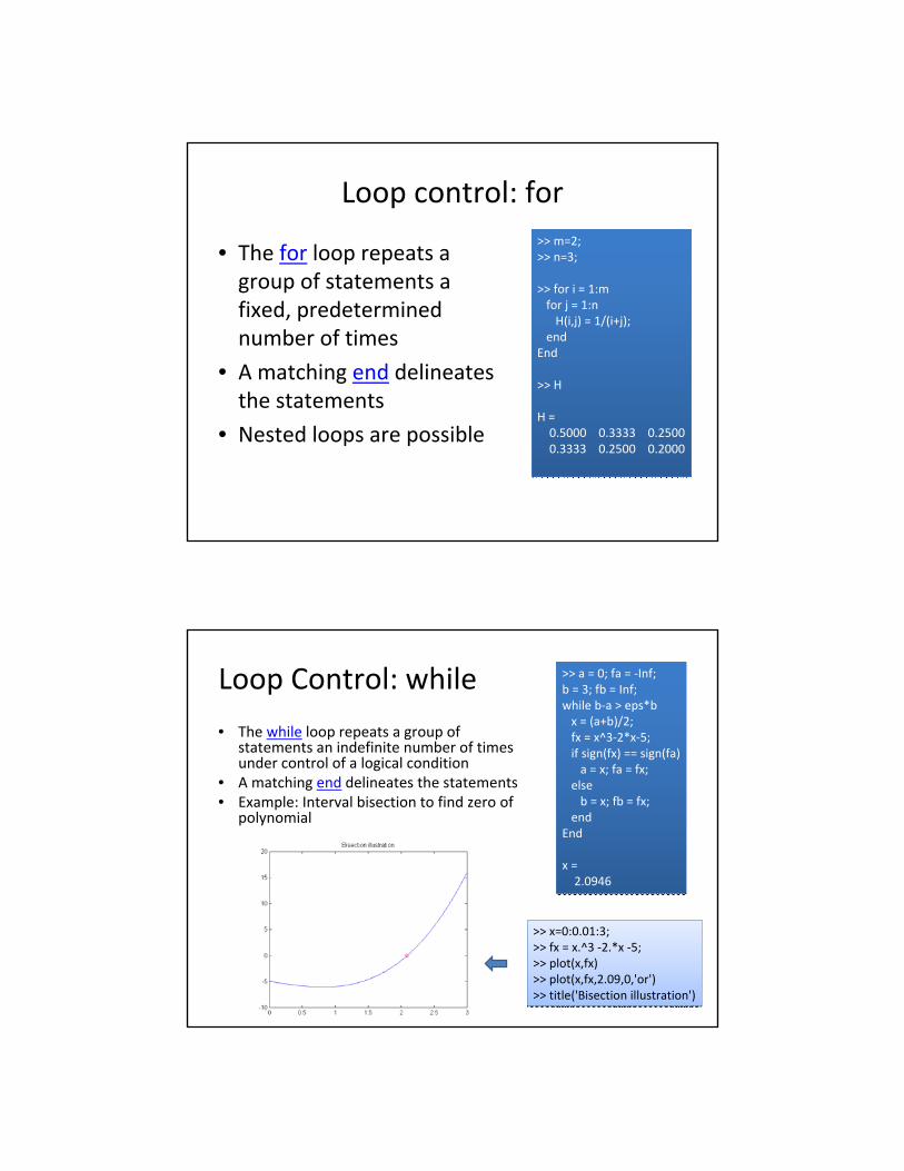
Loop control: for

• The for loop repeats a group of statements a fixed, predetermined number of times

• A matching end delineates the statements

• Nested loops are possible

>> m=2;>> n=3;

>> for i = 1:mfor j = 1:n

H(i,j) = 1/(i+j);end

End

>> H

H =0.5000 0.3333 0.25000.3333 0.2500 0.2000

>> m=2;>> n=3;

>> for i = 1:mfor j = 1:n

H(i,j) = 1/(i+j);end

End

>> H

H =0.5000 0.3333 0.25000.3333 0.2500 0.2000

Loop Control: while

• The while loop repeats a group of statements an indefinite number of times under control of a logical condition

• A matching end delineates the statements• Example: Interval bisection to find zero of

polynomial

>> a = 0; fa = -Inf;b = 3; fb = Inf;while b-a > eps*b

x = (a+b)/2;fx = x^3-2*x-5;if sign(fx) == sign(fa)

a = x; fa = fx;else

b = x; fb = fx;end

End

x =2.0946

>> a = 0; fa = -Inf;b = 3; fb = Inf;while b-a > eps*b

x = (a+b)/2;fx = x^3-2*x-5;if sign(fx) == sign(fa)

a = x; fa = fx;else

b = x; fb = fx;end

End

x =2.0946

>> x=0:0.01:3;>> fx = x.^3 -2.*x -5;>> plot(x,fx)>> plot(x,fx,2.09,0,'or')>> title('Bisection illustration')

>> x=0:0.01:3;>> fx = x.^3 -2.*x -5;>> plot(x,fx)>> plot(x,fx,2.09,0,'or')>> title('Bisection illustration')

Loop Control: continue• The continue statement passes

control to the next iteration of the for loop or while loop in which it appears, skipping any remaining statements in the body of the loop

• The same holds true for continue statements in nested loops

• That is, execution continues at the beginning of the loop in which the continue statement was encountered

• Example: counts the lines of code in the file magic.m, skipping all blank lines and comments

fid = fopen('magic.m','r');count = 0;

while ~feof(fid)line = fgetl(fid);if isempty(line) ||...

strncmp(line,'%',1)...|| ~ischar(line)

continueendcount = count + 1;

End

fprintf('%d lines\n',count);fclose(fid);

fid = fopen('magic.m','r');count = 0;

while ~feof(fid)line = fgetl(fid);if isempty(line) ||...

strncmp(line,'%',1)...|| ~ischar(line)

continueendcount = count + 1;

End

fprintf('%d lines\n',count);fclose(fid);

Loop Control: break

• The break statement lets you exit early from a for loop or while loop. In nested loops, break exits from the innermost loop only

• Example: Improved bisection algorithm

>> a = 0; fa = -Inf;b = 3; fb = Inf;while b-a > eps*b

x = (a+b)/2;fx = x^3-2*x-5;if fx == 0

breakelseif sign(fx) == sign(fa)

a = x; fa = fx;else

b = x; fb = fx;end

End

xx =

2.0946

>> a = 0; fa = -Inf;b = 3; fb = Inf;while b-a > eps*b

x = (a+b)/2;fx = x^3-2*x-5;if fx == 0

breakelseif sign(fx) == sign(fa)

a = x; fa = fx;else

b = x; fb = fx;end

End

xx =

2.0946

Flow Control: Try and return

• try is used for error handling control• return terminates the current sequence of commands

and returns control to the invoking function or to the keyboard– return is also used to terminate keyboard mode (useful for

debugging of M-files)– A called function normally transfers control to the function

that invoked it when it reaches the end of the function.– You can insert a return statement within the called

function to force an early termination and to transfer control to the invoking function

– Return is also useful for debugging

Data Structures

• Multidimensional arrays– More than 2 subscripts– Uniform data

• Cell arrays– Cell arrays in MATLAB

are multidimensional arrays whose elements are copies of other arrays (curly braces{})

>> ones(2,3,2)ans(:,:,1) =

1 1 11 1 1

ans(:,:,2) =1 1 11 1 1

>> ones(2,3,2)ans(:,:,1) =

1 1 11 1 1

ans(:,:,2) =1 1 11 1 1

>> A = magic(4);>> C = {A sum(A) prod(prod(A))}C =

[4x4 double] [1x4 double] [2.0923e+013]

>> C{1}ans =

16 2 3 135 11 10 89 7 6 124 14 15 1

>> C{2}ans =

34 34 34 34

>> A = magic(4);>> C = {A sum(A) prod(prod(A))}C =

[4x4 double] [1x4 double] [2.0923e+013]

>> C{1}ans =

16 2 3 135 11 10 89 7 6 124 14 15 1

>> C{2}ans =

34 34 34 34

Data Structures

• Characters and text– Single quotes for text– Character – Ascii code conversations: char,

double– Example: show printable characters

>> F = reshape(32:127,16,6)'F =

32 33 34 35 36 37 38 39 40 41 42 43 44 45 46 4748 49 50 51 52 53 54 55 56 57 58 59 60 61 62 6364 65 66 67 68 69 70 71 72 73 74 75 76 77 78 7980 81 82 83 84 85 86 87 88 89 90 91 92 93 94 9596 97 98 99 100 101 102 103 104 105 106 107 108 109 110 111

112 113 114 115 116 117 118 119 120 121 122 123 124 125 126 127

>> F = reshape(32:127,16,6)'F =

32 33 34 35 36 37 38 39 40 41 42 43 44 45 46 4748 49 50 51 52 53 54 55 56 57 58 59 60 61 62 6364 65 66 67 68 69 70 71 72 73 74 75 76 77 78 7980 81 82 83 84 85 86 87 88 89 90 91 92 93 94 9596 97 98 99 100 101 102 103 104 105 106 107 108 109 110 111

112 113 114 115 116 117 118 119 120 121 122 123 124 125 126 127

>> char(F)ans =!"#$%&'()*+,-./

0123456789:;<=>?@ABCDEFGHIJKLMNOPQRSTUVWXYZ[\]^_`abcdefghijklmnopqrstuvwxyz{|}~�

>> char(F+128)ans =¡¢£¤¥¦§¨©ª«¬-®¯

°±²³´µ¶·¸¹º»¼½¾¿ÀÁÂÃÄÅÆÇÈÉÊËÌÍÎÏÐÑÒÓÔÕÖ×ØÙÚÛÜÝÞßàáâãäåæçèéêëìíîïðñòóôõö÷øùúûüýþÿ

>> char(F)ans =!"#$%&'()*+,-./

0123456789:;<=>?@ABCDEFGHIJKLMNOPQRSTUVWXYZ[\]^_`abcdefghijklmnopqrstuvwxyz{|}~�

>> char(F+128)ans =¡¢£¤¥¦§¨©ª«¬-®¯

°±²³´µ¶·¸¹º»¼½¾¿ÀÁÂÃÄÅÆÇÈÉÊËÌÍÎÏÐÑÒÓÔÕÖ×ØÙÚÛÜÝÞßàáâãäåæçèéêëìíîïðñòóôõö÷øùúûüýþÿ

>> s = 'Hello's =Hello

>> a = double(s)a =

72 101 108 108 111

>> s = 'Hello's =Hello

>> a = double(s)a =

72 101 108 108 111

Data Structures

• Structures are multidimensional MATLAB arrays with elements accessed by textual field designators, such as

>> S.name = 'Ed Plum';S.score = 83;S.grade = 'B+'

S =

name: 'Ed Plum'score: 83grade: 'B+'

>> S.name = 'Ed Plum';S.score = 83;S.grade = 'B+'

S =

name: 'Ed Plum'score: 83grade: 'B+'

>> S(2).name = 'Miller';S(2).score = 91;S(2).grade = 'A-';

>> S(2).name = 'Miller';S(2).score = 91;S(2).grade = 'A-';

>> S(3) = struct('name','Garcia',... 'score',70,'grade','C')

S =

1x3 struct array with fields:namescoregrade

>> S(3) = struct('name','Garcia',... 'score',70,'grade','C')

S =

1x3 struct array with fields:namescoregrade

Data Structure: Dynamic Field Names

• Normally, access the data in a structure by specifying the name of the field that you want to reference.

• Another means of accessing structure data is to use dynamic field names.

• These names express the field as a variable expression that MATLAB evaluates at run-time. The dot-parentheses syntax shown here makes expression a dynamic field name:– structName.(expression)

Example of Dynamic Field Namesfunction avg = avgscore(testscores, student, first, last) for k = first:last

scores(k) = testscores.(student).week(k); end avg = sum(scores)/(last - first + 1);

function avg = avgscore(testscores, student, first, last) for k = first:last

scores(k) = testscores.(student).week(k); end avg = sum(scores)/(last - first + 1);

>> testscores.Ann_Lane.week(1:25) = ...[95 89 76 82 79 92 94 92 89 81 75 93 ...85 84 83 86 85 90 82 82 84 79 96 88 98];

>> testscores.William_King.week(1:25) = ...[87 80 91 84 99 87 93 87 97 87 82 89 ...86 82 90 98 75 79 92 84 90 93 84 78 81];

>> testscores.Ann_Lane.week(1:25) = ...[95 89 76 82 79 92 94 92 89 81 75 93 ...85 84 83 86 85 90 82 82 84 79 96 88 98];

>> testscores.William_King.week(1:25) = ...[87 80 91 84 99 87 93 87 97 87 82 89 ...86 82 90 98 75 79 92 84 90 93 84 78 81];

Define M-fileavgscore.m with adynamic field name

Create data with corresponding field names

Evaluate function

>> avgscore(testscores, 'Ann_Lane', 7, 22)ans =

85.2500

>> avgscore(testscores, 'William_King', 7, 22)ans =

87.7500

>> avgscore(testscores, 'Ann_Lane', 7, 22)ans =

85.2500

>> avgscore(testscores, 'William_King', 7, 22)ans =

87.7500

Scripts and Functions

• Powerful programming language

• and interactive computational environment

• Files with MATLAB code are called M-files (x.m)

• M-files can be created with text editors

• Two kinds of M-files– Scripts without input or output arguments. They

operate on data in the workspace

– Functions with input arguments and returning output arguments. Internal variables are local to the function

Scripts: Example

• In the current directory write an M-file called cosPlot.m

• In the Command Window type cosPlot

• MATLAB executes the commands

• Variables used remain in the Workspace

• Existing variables in the Workspace can be used

Scripts: Example

Functions

• Functions are M-files that can accept input arguments and return output arguments

• The names of the M-file and of the function should be the same

• Functions operate on variables within their own workspace, separate from the workspace at the MATLAB command prompt.

Example: rank functionfunction r = rank(A,tol)%RANK Matrix rank.% RANK(A) provides an estimate of the number of linearly% independent rows or columns of a matrix A.% RANK(A,tol) is the number of singular values of A% that are larger than tol.% RANK(A) uses the default tol = max(size(A)) * eps(norm(A)).%% Class support for input A:% float: double, single

% Copyright 1984-2007 The MathWorks, Inc.% $Revision: 5.11.4.5 $ $Date: 2007/08/03 21:26:23 $

s = svd(A);if nargin==1

tol = max(size(A)) * eps(max(s));endr = sum(s > tol);

function r = rank(A,tol)%RANK Matrix rank.% RANK(A) provides an estimate of the number of linearly% independent rows or columns of a matrix A.% RANK(A,tol) is the number of singular values of A% that are larger than tol.% RANK(A) uses the default tol = max(size(A)) * eps(norm(A)).%% Class support for input A:% float: double, single

% Copyright 1984-2007 The MathWorks, Inc.% $Revision: 5.11.4.5 $ $Date: 2007/08/03 21:26:23 $

s = svd(A);if nargin==1

tol = max(size(A)) * eps(max(s));endr = sum(s > tol);

>> type rank>> type rank

First line:- keyword ‘function’- output argument r- name of function- input arguments

Followed by commentsthat provide Help text

Function code- variable number of input

and output argumentsgiven by variablesnargin and nargout

Types of Functions

• Anonymous functions– Can be defined without M-files

• Primary and subfunctions– Primary: first function in the M-file– Subfunctions: further functions in M-file but only

visible to functions in M-file• Private functions (see Help)• Nested functions

– Function in function• Function overloading (see Help)

>> sqr = @(x) x.^2;>> a = sqr(5)a =

25

>> b = sqr(1:3)b =

1 4 9

>> sqr = @(x) x.^2;>> a = sqr(5)a =

25

>> b = sqr(1:3)b =

1 4 9

Global Variables

• More than one function and the workspace can share a single copy of a variable

• The global variable has to be declared by the keyword global and must be set before used

function h = falling(t) global GRAVITY h = 1/2*GRAVITY*t.^2;

function h = falling(t) global GRAVITY h = 1/2*GRAVITY*t.^2;

M-file: falling.m

>> global GRAVITY>> GRAVITY = 32;>> y = falling((0:1:5))

y =

0 16 64 144 256 400

>> global GRAVITY>> GRAVITY = 32;>> y = falling((0:1:5))

y =

0 16 64 144 256 400

The eval function

• Powerful text macro facility that can execute MATLAB code in text variables

• Example: Construction of text variables with MATLAB code in a for loop and executing it– loading of files August1.dat August2.dat …

for d = 1:31 s = ['load August' int2str(d) '.dat']; eval(s) % Process the contents of the d-th file

end

for d = 1:31 s = ['load August' int2str(d) '.dat']; eval(s) % Process the contents of the d-th file

end

Function Handles

• Handles can be created to any MATLAB function with the at sign @

• Example: Handle to sin function

• Function handles can also be passed to functions by input arguments

• Example: general plot functions

>> fhandle = @sin;>> fhandle(pi/2)ans =

1

>> fhandle = @sin;>> fhandle(pi/2)ans =

1

function x = plotFunctionHandle(fhandle, data)plot(data, fhandle(data))end

function x = plotFunctionHandle(fhandle, data)plot(data, fhandle(data))end

>> plotFunctionHandle(@sin, -pi:0.01:pi)>> plotFunctionHandle(@cos, -pi:0.01:pi)>> plotFunctionHandle(@sin, -pi:0.01:pi)>> plotFunctionHandle(@cos, -pi:0.01:pi)

M-file: plotFunctionHandle.m

Function Functions

• A class of functions called "function functions" works with nonlinear functions of a scalar variable

• One function works on another function• The function functions include

– Zero finding– Optimization – Quadrature– Ordinary differential equations

Example: Zero Finding

• Demo function: – humps

• Problem: Find zero of function humps

function y = humps(x) y = 1./((x-.3).^2 + .01) + 1./((x-.9).^2 + .04) - 6;function y = humps(x) y = 1./((x-.3).^2 + .01) + 1./((x-.9).^2 + .04) - 6;

M-file: humps.m

>> x = 0:.002:1;y = humps(x);>> plot(x,y)

>> x = 0:.002:1;y = humps(x);>> plot(x,y)

>> p = fminsearch(@humps,.5)p =

0.6370

>> y = humps(p)y =

11.2528>> hold on>> plot(p,y,'or')

>> p = fminsearch(@humps,.5)p =

0.6370

>> y = humps(p)y =

11.2528>> hold on>> plot(p,y,'or')

Vectorization

• One way to make your MATLAB programs run faster is to vectorize the algorithms you use in constructing the programs

x = .01; for k = 1:1001

y(k) = log10(x); x = x + .01;

end

x = .01; for k = 1:1001

y(k) = log10(x); x = x + .01;

end

Bad, slow

x = .01:.01:10; y = log10(x);x = .01:.01:10; y = log10(x);

Good, vectorized, fast

Preallocation

• You can make your for loops go faster by preallocating any vectors or arrays in which output results are stored

for n = 1:32 r(n) = rank(magic(n));

end

for n = 1:32 r(n) = rank(magic(n));

end

Bad, slow, space for r dynamically allocated

Good, fast, space for r preallocated

r = zeros(32,1); for n = 1:32

r(n) = rank(magic(n)); end

r = zeros(32,1); for n = 1:32

r(n) = rank(magic(n)); end

Contents

• Overview of MATLAB System

• Matrices and Arrays

• Programming

• Report Generation

Report Generation with MATLAB

• Two possibilities to generate reports with MATLAB– Publishing M-files to various output formats

• Html, xml, latex, pdf• Doc and ppt on PC only

– Publishing to MS Word with Notebook• On Windows with MS Word installed only• Notebook has to be configured• Notebook creates M-books

– MS Word documents containing text, MATLAB commands and MATLAB output

Applications of Report Generation

• Repeated evaluation of many different input data sets

• Repeated application of complex procedures on input data set by changing parameters and comparing results

• Advantages• Can dramatically increase productivity of people• Uniform representation of results• Less errors• Less resistance to re-evaluate data with slightly changed

conditions

Publishing M-files

• Share your MATLAB code and its results with others

• Published M-files include– Formatted text, numbered lists, Tex equations …– MATLAB code– Results of code evaluation such as figures and output

of command window

• Structure an existing M-file with cells and comments using text markup and publish it in your preferred format

Elements of Publishing M-files

• Cell: Section of code to be presented as titled subsection in the published document– The double percent signs (%%) indicate the

start of a new cell. The text behind is the title

– A single percent sign indicates the beginning of a comment line

%% Square Waves from Sine Waves % The Fourier series expansion for a square-wave is % made up of a sum of odd harmonics, as shown here % using MATLAB(R).

%% Square Waves from Sine Waves % The Fourier series expansion for a square-wave is % made up of a sum of odd harmonics, as shown here % using MATLAB(R).

% % $$ y = y + \frac{sin(k*t)}{k} $$%

% % $$ y = y + \frac{sin(k*t)}{k} $$%

Comment with TeX equation

Examples of Report Generation

• With Notebook: Demo– Computation of sacroiliac corridors in CT-data of

the pelvis– MS Word document with Principal Components

Analysis

• With M-files: Exercise– MATLAB / User Guide / Desktop Tools and

Development Environment / Publishing M-Files / Overview of Publishing M-Files / Example of a Published M-File