Introduction to Mathematical Methods in Neurobiology:

Dynamical Systems

Oren Shriki

2009

Modeling Conductance-Based Networks by Rate Models 1

References:

• Shriki, Hansel, Sompolinsky, Neural Computation 15, 1809–1841 (2003)

• Tuckwell, HC. Introduction to Theoretical Neurobiology, I&II, Cambridge UP, 1988.

2

Conductance-Based Models vs. Simplified Models

• There are two main classes of theoretical approaches to the behavior of neural systems:

– Simulations of detailed biophysical models.

– Analytical (and numerical) solutions of simplified models (e.g. Hopfield models, rate models).

• Simplified models are extremely useful for studying the collective behavior of large neuronal networks. However, it is not always clear when they provide a relevant description of the biological system, and what meaning can be assigned to the quantities and parameters used in them.

3

Conductance-Based Models vs. Simplified Models

• Using mean-field theory we can describe the dynamics of a conductance-based network in terms of firing-rates rather than voltages.

• The analysis will lead to a biophysical interpretation of the parameters that appear in classical rate models.

• The analysis will be divided into two parts:

– A. Steady-state analysis (constant firing rates)

– B. Firing-rate dynamics

4

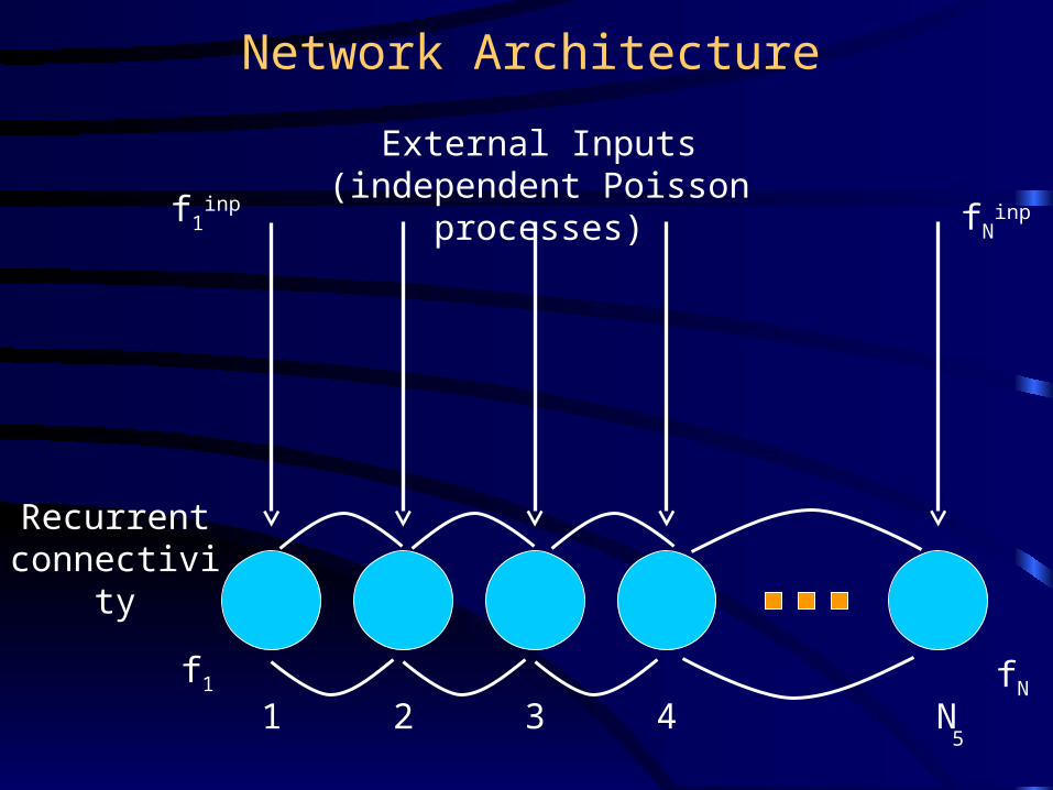
Network Architecture

External Inputs (independent Poisson processes)

Recurrent connectivity

1 2 3 4 N

f1inp

f1

fNinp

fN

5

Voltage Dynamics for A Network of Conductance-Based Point Neurons

We assume that the neurons are point neurons obeying Hodgkin-Huxley type dynamics:

• Iactive – Ionic current involved in the action potential• Iext – External synaptic inputs• Inet – Synaptic inputs from within the network• Iapp – External current applied by the experimentalist

),,1( )( NiIIIIEtVgdt

dVC app

ineti

exti

activeiLiL

im

6

tt_spike

sg t

G

s

A spike at time tspike of the presynaptic cell contributes to the postsynaptic cell a time-depndent conductance , gs(t):

Synaptic Conductances

Peak conductance

7

Synaptic Dynamics: An Example• Synaptic dynamics are usually characterized by

fast rise and slow decay.

• The simplest model assumes instantaneous rise and exponential decay:

)(tGRg

dt

dg ss

spiket

spiketttR )( (Presynaptic rate)

8

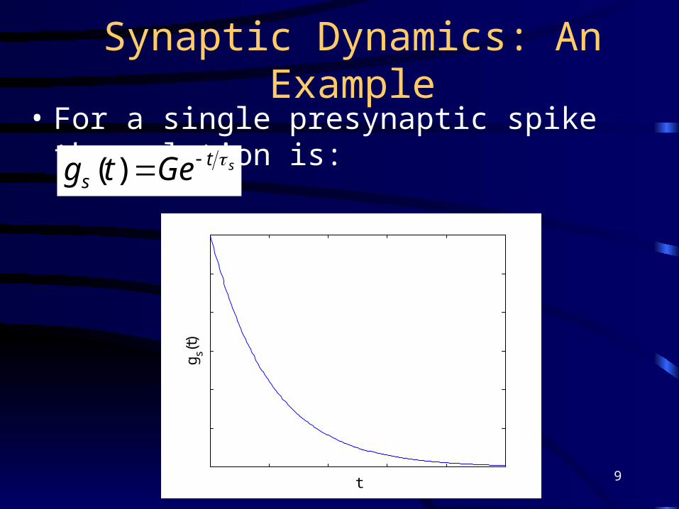
Synaptic Dynamics: An Example• For a single presynaptic spike the solution is:

sts Getg )(

t

g s(t)

9

Synaptic Dynamics: An Example• Implementation in numerical simulations:

• Given the time step dt define the attenuation factor:

• A dimensionless parameter, f, is increased by 1 after each presynaptic spike and multiplied by the attenuation factor in each time step.

• The conductance is the product of f and the peak conductance, G.

sdtdt ee

10

Synaptic Dynamics• For simplicity, we shall write in general:

• K(t) is the time course (dimensionless) function.

• We define:

• For example:

)()( tGKtgs

0

)( dttKs

st

st ss edte

0

0 11

External Synaptic Current

• The explicit expression for the external synaptic current is:

• The peak synaptic conductance is:

• The time constant is:

inpiG

inpi

)()()( tVEtgtI iinpinp

iexti

12

Internal Synaptic Current

• The explicit expression for the internal synaptic current is:

• The peak synaptic conductance is:

• The time constant is:

ijG

ij

N

jijij

neti tVEtgtI

1

)()()(

13

Part A: Steady-State Analysis

The main assumptions are:

• Firing rates of external inputs are constant in time

• Firing rates within the network are constant in time

• The network state is asynchronous

• The network contains many neurons

14

Asynchronous States in Large Networks

• In large asynchronous networks each neuron is bombarded by many synaptic inputs at any moment.

• The fluctuations in the total input synaptic conductance around the mean are relatively small.

• Thus, the total synaptic conductance in the input to each neuron is (approximately) constant.

15

Asynchronous States in Large Networks

• The figure below shows the synaptic conductance of a certain postsynaptic neuron in a simulation of two interacting populations (excitatory and inhibitory):

16

Mean-Field Approximation

• We can substitute the total synaptic conductance by its mean value.

• This approximation is called the “Mean-Field” (MF) Approximation.

• The justification for the MF approximation is the central limit theorem.

17

The Central Limit Theorem

• A random variable ,which is the sum of many independent random variables, has a Gaussian distribution with mean value equal to the sum of the mean values of the individual random variables.

• The ratio between the standard deviation and the mean of the sum satisfies:

where N is the number of individual random variables.

Nmean

std 1

18

Mean-Field Analysis of the Synaptic Inputs

• The total contribution to the i’th neuron from within the network is:

• The contribution to this sum from the j’th neuron is:

N

j tjijij

N

jij

neti

j

ttKGtgtg11

)()(

jt

jijijij ttKGtg )(

19

Mean-Field Analysis of the Synaptic Inputs

• Consider a time window T>>1/fj, where fj is the firing rate of the presynaptic neuron j.

• Schematically, the contribution of the j’th neuron in this time window looks like this:

)(tgij

Tt

ijg

spikes

Tt

20

Mean-Field Analysis of the Synaptic Inputs

• The mean conductance due to the j’th neuron over a long time window is:

• The mean conductance resulting from all neurons in the network is:

jijij

ijijspike

T

ijij

fG

dttKGT

TNdttg

Tg

00

)()(

)(1

N

jjijij

N

jij

neti fGgg

11

21

Mean-Field Analysis of the Synaptic Inputs

• The mean-field approximation is:

• Effectively, we replace a spatial averaging by a temporal averaging .

• Using a similar analysis, the contribution of the external inputs can be replaced by:

N

jjijij

neti

neti fGgtg

1

)(

inpi

inpi

inpi

exti

exti fGgtg )(

22

Mean-Field Analysis of the Synaptic Inputs

• The synaptic currents are not constant in time since the voltage of the neuron varies significantly over time:

• We can decompose the last expression in the following way:

N

jijij

neti tVEtgtI

1

)()()(

N

jijLi

N

jLjij

N

jiLLjij

neti

tgEtVEEtg

tVEEEtgtI

11

1

)()()(

)()()(

23

Mean-Field Analysis of the Synaptic Inputs

• We now use the MF approximation :

• This gives: Lj

N

jjijij

N

jLjij

N

jjijij

neti

N

jij

EEfGEEtg

fGtgtg

11

11

)(

)()(

N

jjijijLijLj

N

jijij

neti fGEtVfEEGtI

11

)()(

A constant applied current

A constant increase in the leak conductance 24

Mean-Field Analysis of the Synaptic Inputs

• Similarly:

• We obtained the following mapping:

inpi

inpi

inpiLi

inpiL

inpi

inpi

inpi

exti fGEtVfEEGtI )()(

inpi

inpi

inpi

N

jjijijLL

inpiL

inpi

inpi

inpijLj

N

jijij

appi

appi

fGfGgg

fEEGfEEGII

1

1

25

Mean-Field Analysis of the Synaptic Inputs

• To sum up:• Asynchronous Synaptic Inputs Produce a Stationary Shift in

the Voltage-Independent Currentand in the Input Passive Conductanceof the Postsynaptic Cell.

• To complete the loop and determine the network’s firing rates we need to know how the firing rate of a single cell is affected by these shifts.

26

Current-Frequency Response Curves of Cortical Neurons are Semi-Linear

Excitatory Neuron (After: Ahmed et. al., Cerebral Cortex 8, 462-476, 1998):

Inhibitory Neurons (After: Azouz et. al., Cerebral Cortex 7, 534-545, 1997) :

27

The Effect of Changing the Input Conductance is Subtractive

Experiment:

f-I curves of a cortical neuron before and after iontophoresis

of baclofen, which opens synaptic conductances.

(Connors B. et. al., Progress in Brain Research, Vol. 90, 1992).

28

A Hodgkin-Huxley Neuron with an A-current

b

n

h

/τ(V)-mbdb/dt

/τ(V)-nndn/dt

/τ(V)-hhdh/dt

)(, tIwVIdt

dVC ion

)()()()(

,,,

LL3

K4

KNa3

Na EVgEVbagEVngEVhmg

nhmVI

KA

ion

29

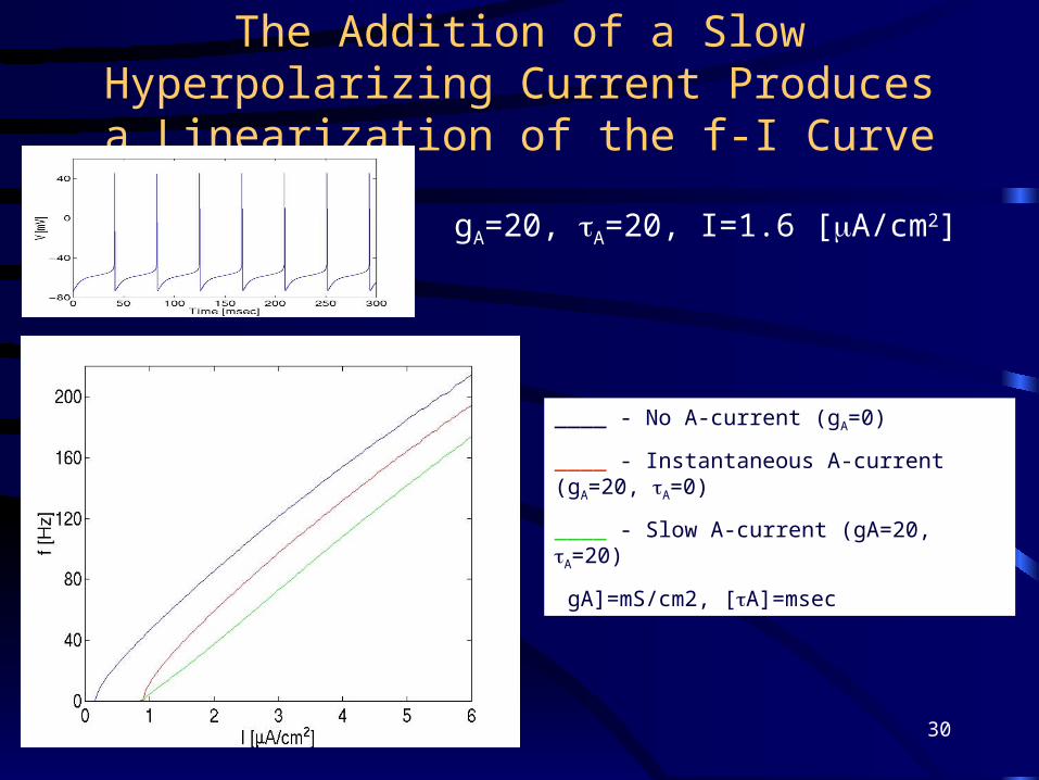
The Addition of a Slow Hyperpolarizing Current Produces a Linearization of the f-I Curve

____ - No A-current (gA=0)

____ - Instantaneous A-current (gA=20, A=0)

____ - Slow A-current (gA=20, A=20)

[gA]=mS/cm2, [A]=msec

gA=20, A=20, I=1.6 [A/cm2]

30

The Effect of Increasing gL is Subtractive

31

Model Equations with Parameters:

Shriki et al., Neural Computation 15, 1809–1841 (2003)

32

The Dependence of the Firing Rate on I and on gL Can Be Described by a Simple Phenomenological Model

LcC

C

gVII

IIf0

[x]+=x if x>0 and 0 otherwise.

We find for the model neuron :

=35.4 [Hz/(A/cm2)]Vc=5.6 [mV]IC

0=0.65 [A/cm2] 33

The Effect of the Synaptic Input On the Firing Rate

Combining the previous results, we find that the steady-state firing rates obey the following equations:

LccjcLj

N

jijij

inpicL

inpi

inpi

inpi

appii

gVIfVEEG

fVEEGIf

0

1

34

The Effect of the Synaptic Input On the Firing Rate

c

N

jjij

inpi

inpi

appii IfJfJIf

1

This can be written us:

Where:

cL

inpi

inpi

inpi

inpi

cLjijijij

VEEGJ

VEEGJ

35

The Units of the Interactions

• The units of J are units of electric charge:

• The quantity Jijfj reflects the mean current due to the j’th synaptic source.

• The strength of the interaction Jij reflects the amount of charge that is transferred with each presynaptic action potential.

CQtIVtgJ

36

E Eij ij ij s L cJ G E E V

s L cE E V

s L cE E V

‘‘excitatoryexcitatory’’

‘‘inhibitoryinhibitory’’

The Sign of the Interaction

• The interaction strength in the rate model has the form:

• The rule for excitation / inhibition is:

• This does not necessarily coincide with the biological definition of excitation/inhibition.

37

The Sign of the Interaction

• The biological definition is:

• A positive J implies that this synaptic source increases the firing rate.

• In general, it may be that a certain synaptic source tends to elicit a spike but increases the conductance in a way that reduces the overall firing rate.

sE

sE

excitatoryexcitatory

inhibitoryinhibitory

38

The Model Parameters

• Neuron:

• β – Slope of frequency-current response

• Vc, Ic0 – Dependence of current threshold on leak

conductance

• EL – Reversal potential of leak conductance

• Synapse:

• Gij – Peak synaptic conductance

• Ej – Synaptic reversal potential

• τij – Synaptic time constant 39

ccinpinp IJfNfJf

cinpinp

c

IfJJN

f

1

Rate Model for a Homogeneous, Highly Connected Excitatory Network:

40

Simulations of the Excitatory Network and Rate Model Prediction

41