Introduction to Machine Learning - CmpE WEB
20
ETHEM ALPAYDIN © The MIT Press, 2010 [email protected] http://www.cmpe.boun.edu.tr/~ethem/i2ml2e Lecture Slides for
Transcript of Introduction to Machine Learning - CmpE WEB
ETHEM ALPAYDIN© The MIT Press, 2010
[email protected]://www.cmpe.boun.edu.tr/~ethem/i2ml2e
Lecture Slides for


Introduction Modeling dependencies in input; no longer iid
Sequences:
Temporal: In speech; phonemes in a word (dictionary), words in a sentence (syntax, semantics of the language).
In handwriting, pen movements
Spatial: In a DNA sequence; base pairs
3Lecture Notes for E Alpaydın 2010 Introduction to Machine Learning 2e © The MIT Press (V1.0)
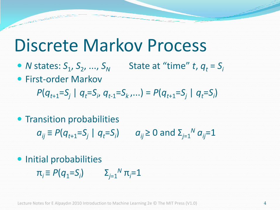
Discrete Markov Process N states: S1, S2, ..., SN State at “time” t, qt = Si
First-order Markov
P(qt+1=Sj | qt=Si, qt-1=Sk ,...) = P(qt+1=Sj | qt=Si)
Transition probabilities
aij ≡ P(qt+1=Sj | qt=Si) aij ≥ 0 and Σj=1N aij=1
Initial probabilities
πi ≡ P(q1=Si) Σj=1N πi=1
4Lecture Notes for E Alpaydın 2010 Introduction to Machine Learning 2e © The MIT Press (V1.0)
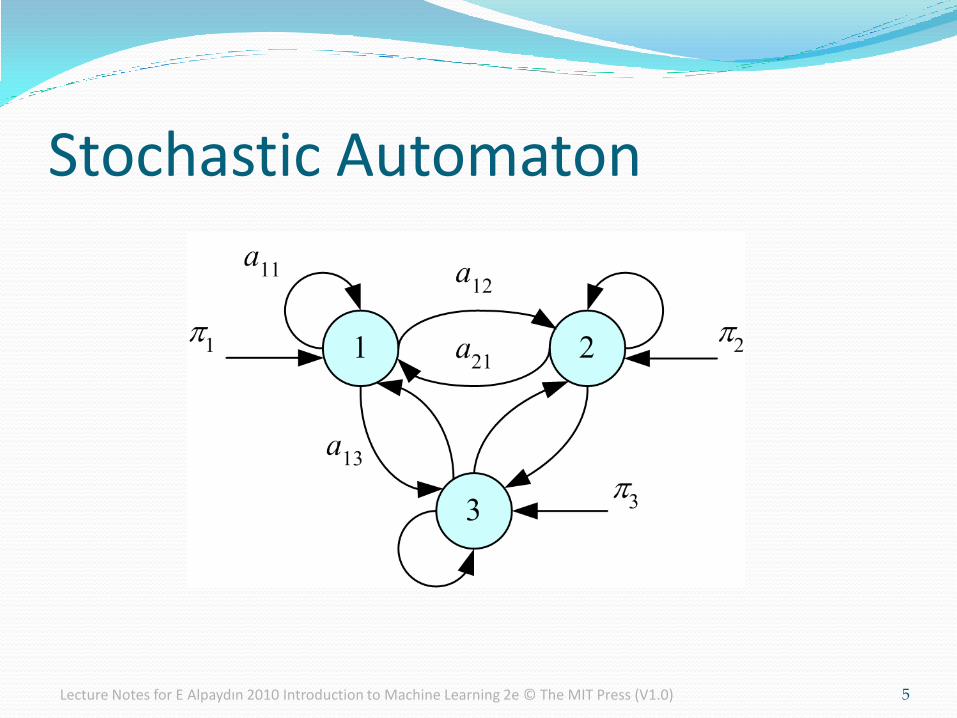
Stochastic Automaton
TT qqqqq
T
t
tt aaqqPqP,QOP1211
2
11 ||
A
5Lecture Notes for E Alpaydın 2010 Introduction to Machine Learning 2e © The MIT Press (V1.0)
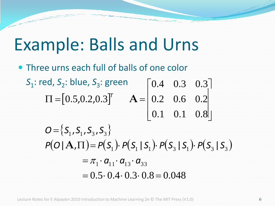
Three urns each full of balls of one color
S1: red, S2: blue, S3: green
Example: Balls and Urns
048080304050
801010
206020
303040
302050
3313111
3313111
3311
.....
|||,|
,,,
...
...
...
.,.,.
aaa
SSPSSPSSPSPOP
SSSSO
T
A
A
6Lecture Notes for E Alpaydın 2010 Introduction to Machine Learning 2e © The MIT Press (V1.0)
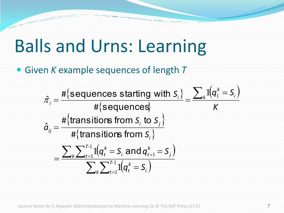
Given K example sequences of length T
Balls and Urns: Learning
k
T-
t ikt
k
T-
t jkti
kt
i
ji
ij
k ik
ii
Sq
SqSq
S
SSa
K
SqS
1
1
1
1 1
1
1
1
1
and
from stransition
to from stransition
sequences
withstarting sequences
#
#ˆ
#
#
7Lecture Notes for E Alpaydın 2010 Introduction to Machine Learning 2e © The MIT Press (V1.0)
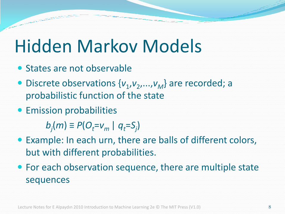
Hidden Markov Models States are not observable
Discrete observations {v1,v2,...,vM} are recorded; a probabilistic function of the state
Emission probabilities
bj(m) ≡ P(Ot=vm | qt=Sj)
Example: In each urn, there are balls of different colors, but with different probabilities.
For each observation sequence, there are multiple state sequences
8Lecture Notes for E Alpaydın 2010 Introduction to Machine Learning 2e © The MIT Press (V1.0)
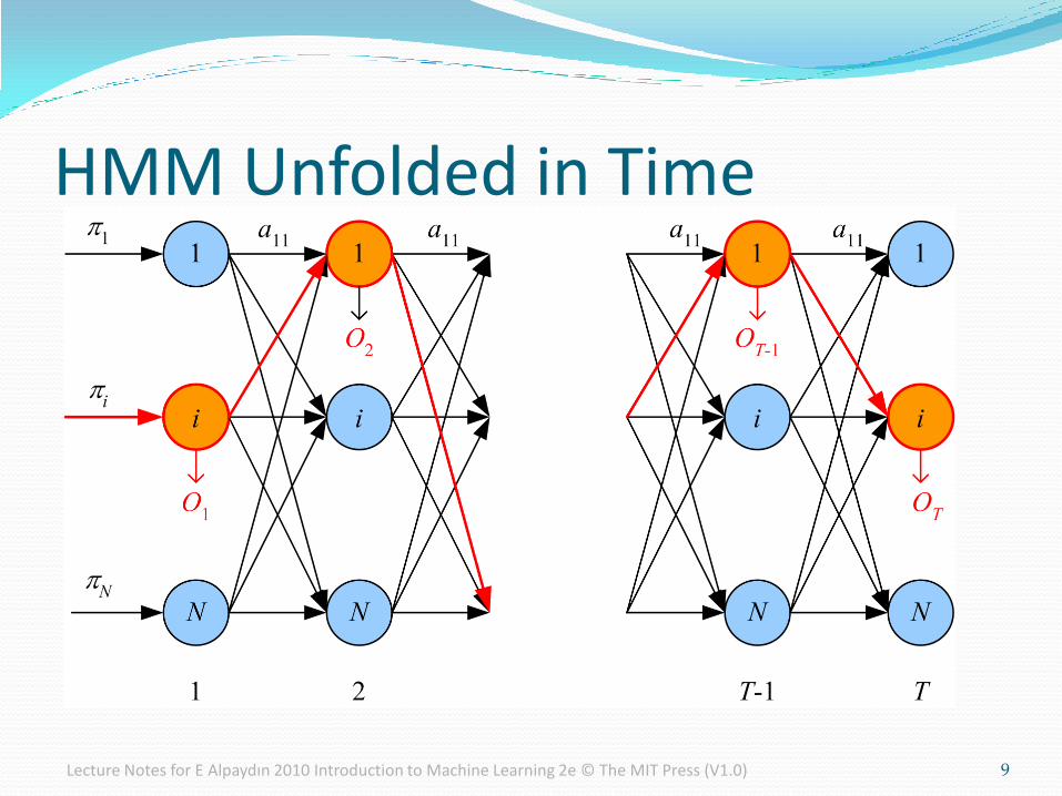
HMM Unfolded in Time
9Lecture Notes for E Alpaydın 2010 Introduction to Machine Learning 2e © The MIT Press (V1.0)

Elements of an HMM N: Number of states
M: Number of observation symbols
A = [aij]: N by N state transition probability matrix
B = bj(m): N by M observation probability matrix
Π = [πi]: N by 1 initial state probability vector
λ = (A, B, Π), parameter set of HMM
10Lecture Notes for E Alpaydın 2010 Introduction to Machine Learning 2e © The MIT Press (V1.0)

Three Basic Problems of HMMs1. Evaluation: Given λ, and O, calculate P (O | λ)
2. State sequence: Given λ, and O, find Q* such that
P (Q* | O, λ ) = maxQ P (Q | O , λ )
3. Learning: Given X={Ok}k, find λ* such that
P ( X | λ* )=maxλ P ( X | λ )
11
(Rabiner, 1989)
Lecture Notes for E Alpaydın 2010 Introduction to Machine Learning 2e © The MIT Press (V1.0)

Forward variable:
Evaluation
N
iT
tj
N
iijtt
ii
ittt
iOP
Obaij
Obi
SqOOPi
1
1
1
1
11
1
|
:Recursion
:tionInitializa
|,
12Lecture Notes for E Alpaydın 2010 Introduction to Machine Learning 2e © The MIT Press (V1.0)
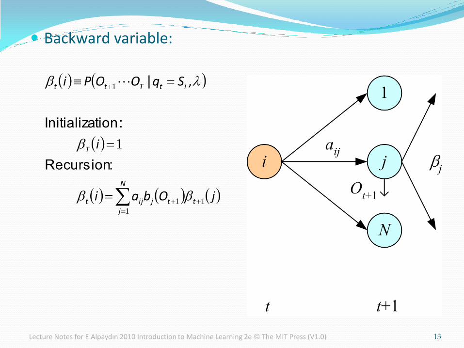
Backward variable:
N
jttjijt
T
itTtt
jObai
i
SqOOPi
1
11
1
1
:Recursion
:tionInitializa
| ,
13Lecture Notes for E Alpaydın 2010 Introduction to Machine Learning 2e © The MIT Press (V1.0)

Finding the State Sequence
14
N
j tt
tt
itt
jj
ii
OSqPi
1
,
No!
Choose the state that has the highest probability, for each time step:
qt*= arg maxi γt(i)
Lecture Notes for E Alpaydın 2010 Introduction to Machine Learning 2e © The MIT Press (V1.0)

Viterbi’s Algorithm
δt(i) ≡ maxq1q2∙∙∙ qt-1
p(q1q2∙∙∙qt-1,qt =Si,O1∙∙∙Ot | λ)
Initialization: δ1(i) = πibi(O1), ψ1(i) = 0
Recursion:δt(j) = maxi δt-1(i)aijbj(Ot), ψt(j) = argmaxi δt-1(i)aij
Termination:p* = maxi δT(i), qT
*= argmaxi δT (i) Path backtracking:
qt* = ψt+1(qt+1
* ), t=T-1, T-2, ..., 1
15Lecture Notes for E Alpaydın 2010 Introduction to Machine Learning 2e © The MIT Press (V1.0)
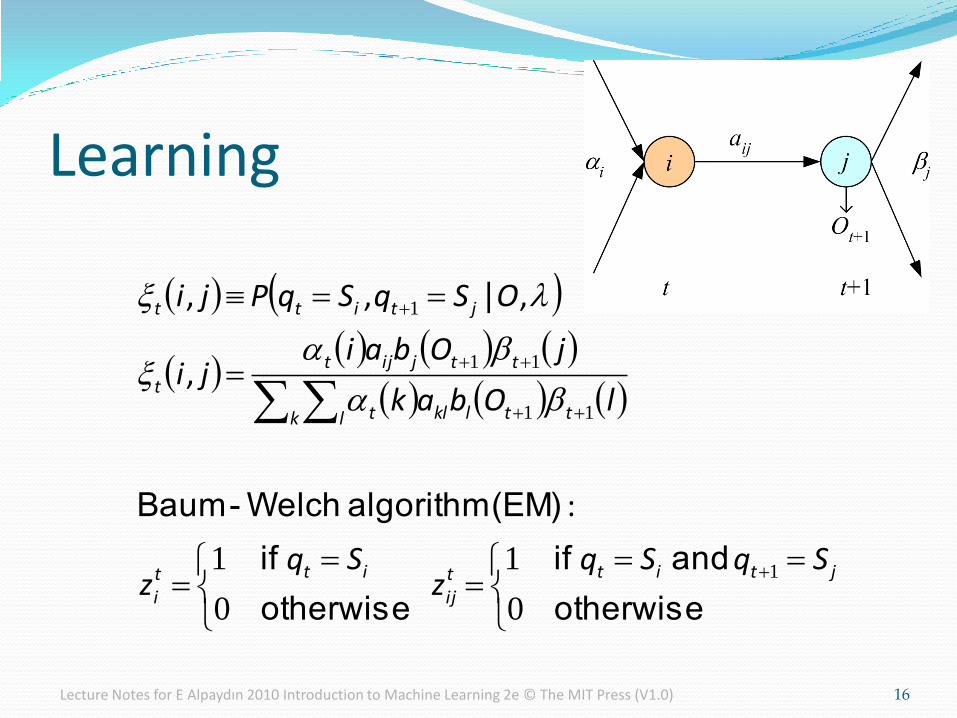
Learning
16
otherwise
and if
otherwise
if
(EM) algorithm Welch-Baum
|
0
1
0
1 1
11
11
1
jtittij
itti
k l ttlklt
ttjijt
t
jtitt
SqSqz
Sqz
lObak
jObaiji
OSqSqPji
:
,
,,,
Lecture Notes for E Alpaydın 2010 Introduction to Machine Learning 2e © The MIT Press (V1.0)

Baum-Welch (EM)
ˆ
,ˆ ˆ
:s tepM
, :s tepE
K
k
T
t
kt
K
k
T
t mkt
kt
j
K
k
T
t
kt
K
k
T
t
kt
ij
K
k
k
i
ttijt
ti
k
k
k
k
i
vOjmb
i
jia
K
i
jizEizE
1
1
1
1
1
1
1
1
1
1
1
11
1
1
17Lecture Notes for E Alpaydın 2010 Introduction to Machine Learning 2e © The MIT Press (V1.0)
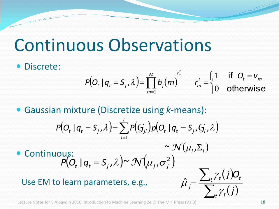
Continuous Observations
2
jjjtt SqOP ,~,| N
18
Discrete:
Gaussian mixture (Discretize using k-means):
Continuous:
otherwise
if |
0
1
1
mttm
rM
mjjtt
vOrmbSqOP
tm
,
ll
ljtt
L
ljljtt SqOpPSqOP
,~
,,| ,|
N
GG1
Use EM to learn parameters, e.g.,
t t
t tt
jj
Oj
Lecture Notes for E Alpaydın 2010 Introduction to Machine Learning 2e © The MIT Press (V1.0)
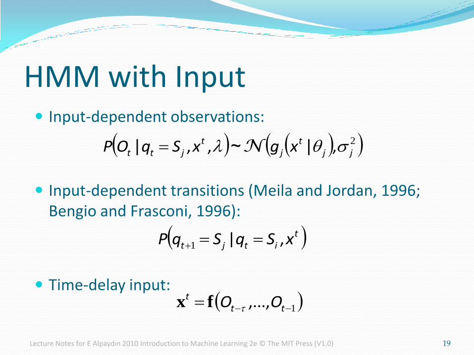
Input-dependent observations:
Input-dependent transitions (Meila and Jordan, 1996; Bengio and Frasconi, 1996):
Time-delay input:
HMM with Input
titjt xSqSqP ,| 1
19
2
jjt
jt
jtt xgxSqOP ,,, |~| N
1 ttt OO ,...,fx
Lecture Notes for E Alpaydın 2010 Introduction to Machine Learning 2e © The MIT Press (V1.0)
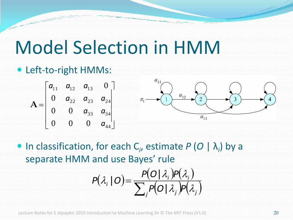
Left-to-right HMMs:
In classification, for each Ci, estimate P (O | λi) by a separate HMM and use Bayes’ rule
Model Selection in HMM
44
3433
242322
131211
000
00
0
0
a
aa
aaa
aaa
A
20
j jj
iii
POP
POPOP
|
||
Lecture Notes for E Alpaydın 2010 Introduction to Machine Learning 2e © The MIT Press (V1.0)