Introduction to Lattice Gauge Theories...

Introduction to Lattice Gauge Theories I

M. Muller-Preussker

Humboldt-University Berlin, Department of Physics

Dubna International Advanced School of Theoretical Physics -

Helmholtz International Summer School

”Lattice QCD, Hadron Structure and Hadronic Matter”

August 25 - September 5, 2014

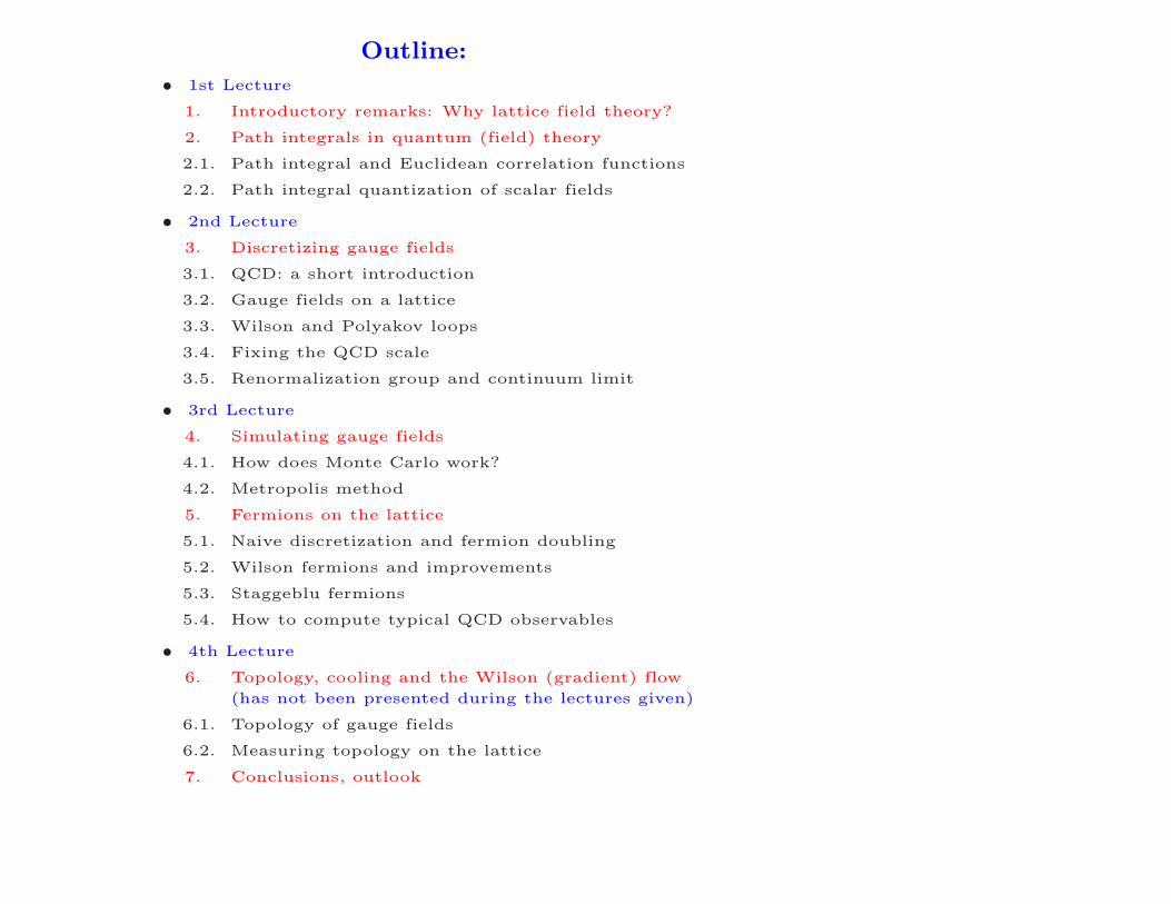
Outline:

• 1st Lecture

1. Introductory remarks: Why lattice field theory?

2. Path integrals in quantum (field) theory

2.1. Path integral and Euclidean correlation functions

2.2. Path integral quantization of scalar fields

• 2nd Lecture

3. Discretizing gauge fields

3.1. QCD: a short introduction

3.2. Gauge fields on a lattice

3.3. Wilson and Polyakov loops

3.4. Fixing the QCD scale

3.5. Renormalization group and continuum limit

• 3rd Lecture

4. Simulating gauge fields

4.1. How does Monte Carlo work?

4.2. Metropolis method

5. Fermions on the lattice

5.1. Naive discretization and fermion doubling

5.2. Wilson fermions and improvements

5.3. Staggeblu fermions

5.4. How to compute typical QCD observables

• 4th Lecture

6. Topology, cooling and the Wilson (gradient) flow

(has not been presented during the lectures given)

6.1. Topology of gauge fields

6.2. Measuring topology on the lattice

7. Conclusions, outlook

Literature, text books:Path integrals:

• R.P. Feynman, A.R. Hibbs, Quantum mechanics and path integrals, Mc Graw Hill, 1965

• L.D. Faddeev, in Methods in field theory, Les Houches School, 1975

• V. Popov, Kontinualniye integraly v kvantovoi teorii polya i statisticheskoi fizikye, Moskva Atomizdat,

1976

• H. Kleinert, Path integrals in quantum mechanics, statistics, polymer physics, World Scientific

• G. Roepstorf, Path integral approach to quantum physics, Springer

• J. Zinn-Justin, Path integrals in quantum mechanics, Oxford University Press (2005), translated

into russian

Lattice field theory:

• K. G. Wilson, Confinement of Quarks, Phys. Rev. D10 (1974) 2445

• J. Kogut, L. Susskind, Hamiltonian Formulation of Wilson’s Lattice Gauge Theories., Phys. Rev.

D11 (1975) 395

• M. Creutz, Quarks, gluons and lattices, Cambrigde Univ. Press (1983), translated into russian

• H. Rothe, Lattice gauge theories - An introduction, World Scientific (4th ed. 2012)

• I. Montvay, G. Munster, Quantum fields on a lattice, Cambrigde Univ. Press

• J. Smit, Introduction to quantum fields on a lattice: A robust mate, Cambridge Lect. Notes Phys. 15

(2002) 1-271

• C. Davies, Lattice QCD, Lecture notes, hep-ph/0205181 (2002)

• A. Kronfeld, Progress in lattice QCD, Lecture notes, hep-ph/0209231 (2002)

• T. DeGrand, C. E. DeTar, Lattice methods for quantum chromodynamics, World Scientific (2006)

• C. Gattringer, C.B. Lang, Quantum Chromodynamics on the Lattice - An introductory presentation,

Springer (2010)

More general on non-perturbative methods:

• Yu. Makeenko, Methods of contemporary gauge theory, Cambrigde Univ. Press (2002)

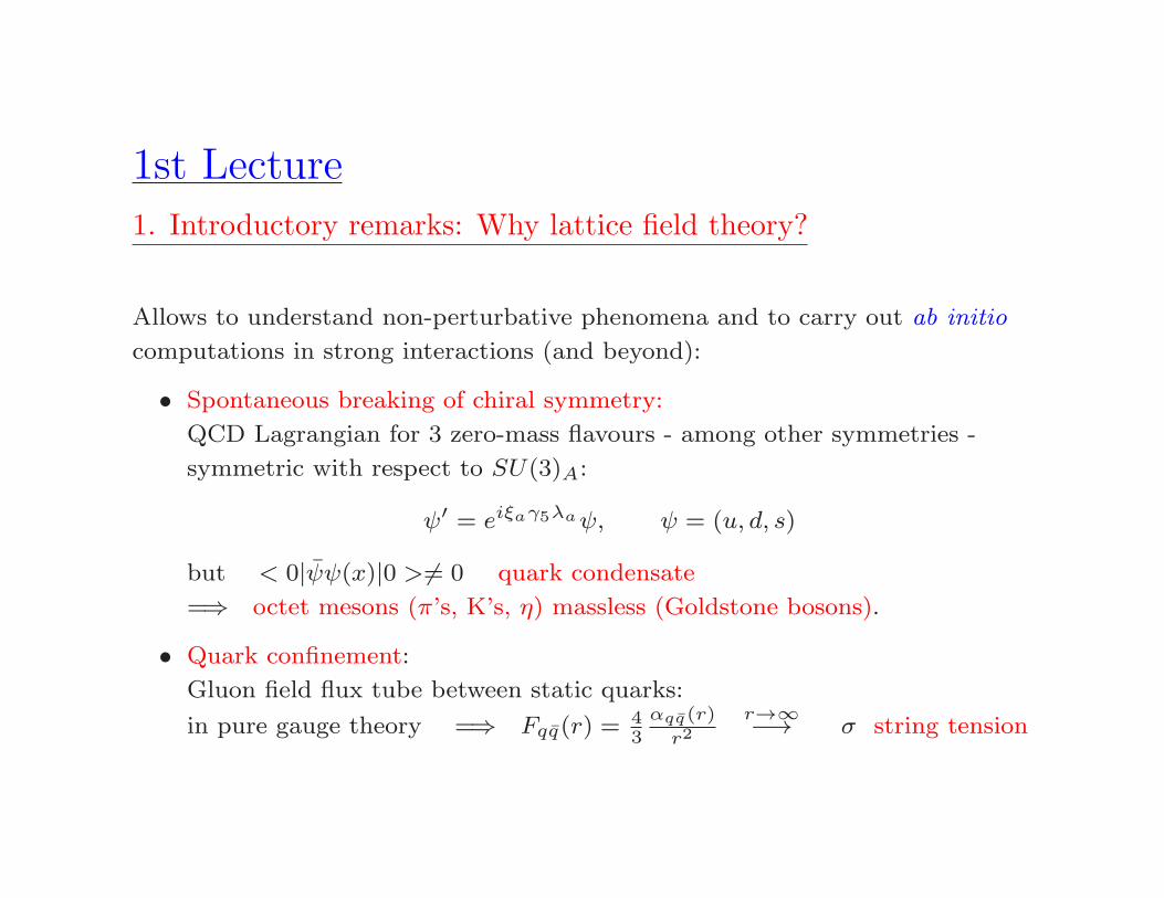
1st Lecture

1. Introductory remarks: Why lattice field theory?

Allows to understand non-perturbative phenomena and to carry out ab initio

computations in strong interactions (and beyond):

• Spontaneous breaking of chiral symmetry:

QCD Lagrangian for 3 zero-mass flavours - among other symmetries -

symmetric with respect to SU(3)A:

ψ′ = eiξaγ5λaψ, ψ = (u, d, s)

but < 0|ψψ(x)|0 > 6= 0 quark condensate

=⇒ octet mesons (π’s, K’s, η) massless (Goldstone bosons).

• Quark confinement:

Gluon field flux tube between static quarks:

in pure gauge theory =⇒ Fqq(r) =43

αqq(r)

r2r→∞−→ σ string tension

Scenarios for confinement made ‘visible’ in lattice QCD:

- flux tube structure visualized

From Abelian projection of SU(2) LGT [Bali, Schilling, Schlichter, ’97]

- condensation of U(1) monopoles: dual superconductor

’t Hooft; Mandelstam; Schierholz,. . ..; Bali, Bornyakov, M.-P., Schilling;

Di Giacomo,. . .; . . .

- center vortices

’t Hooft; Mack; Greensite, Faber, Olejnik; Reinhardt,. . .; Polikarpov,. . .; . . .

- semiclassical approach via instantons, calorons, dyons · · ·solving e.g. the problem of large η′-mass (“UA(1)-problem”)

better understood on the lattice, but responsibility for confinement ???

but cf. lecture by V. Bornyakov

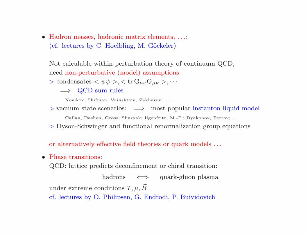
• Hadron masses, hadronic matrix elements, . . .:

(cf. lectures by C. Hoelbling, M. Gockeler)

Not calculable within perturbation theory of continuum QCD,

need non-perturbative (model) assumptions

⊲ condensates < ψψ >,< trGµνGµν >, · · ·=⇒ QCD sum rules

Novikov, Shifman, Vainshtein, Zakharov; . . .

⊲ vacuum state scenarios: =⇒ most popular instanton liquid model

Callan, Dashen, Gross; Shuryak; Ilgenfritz, M.-P.; Dyakonov, Petrov; . . .

⊲ Dyson-Schwinger and functional renormalization group equations

or alternatively effective field theories or quark models . . .

• Phase transitions:

QCD: lattice predicts deconfinement or chiral transition:

hadrons ⇐⇒ quark-gluon plasma

under extreme conditions T, µ, ~B

cf. lectures by O. Philipsen, G. Endrodi, P. Buividovich

• Standard model and beyond:

Non-perturbative lattice approach very useful also for

– strongly coupled QED Kogut,. . .; Schierholz,. . .; Mitrjushkin, M.-P.,. . .; . . .

– Higgs-Yukawa model =⇒ e.g. bounds for Higgs mass

K. Jansen,. . .; J. Kuti,. . .; . . . ,

– (broken) SUSY

cf. lecture notes HISS school 2011 by D. Kazakov, S. Catteral

– lattice studies (large Nc, Nf ) motivated by string theory and AdS/CFT

correspondence M. Teper,. . .; J. Kuti,. . .; V. Zakharov,. . .; . . .

– . . .

2. Path integrals in quantum (field) theory

2.1. Path integral and Euclidean correlation functions

Quantum physics mostly starts from hermitean, time-independent Hamiltonian

H|n〉 = En|n〉, n = 0, 1, 2, . . . with 〈m|n〉 = δm,n,∑

n

|n〉〈n| = 1 .

Schrodinger Equation for time evolution:

i~d

dt|ψ(t)〉 = H|ψ(t)〉 , |ψ(t)〉 = e−

i~H(t−t0)|ψ(t0)〉 .

or

ψ(x, t) ≡ 〈x|ψ(t)〉 =∫

dx0 〈x|e− i~H(t−t0)|x0〉〈x0|ψ(t0)〉 .

Standard task: find En, in particular ground state energy E0.

Useful quantity for this: quantum statistical partition function:

Z = tr(

e−βH)

=

∫

dx 〈x|e−βH |x〉 =⇒ free energy F (V, T ) = −kT logZ, β ≡ 1

kBT

Note formal replacement: real time i~t ↔ imaginary time β ≡ 1

kBT.

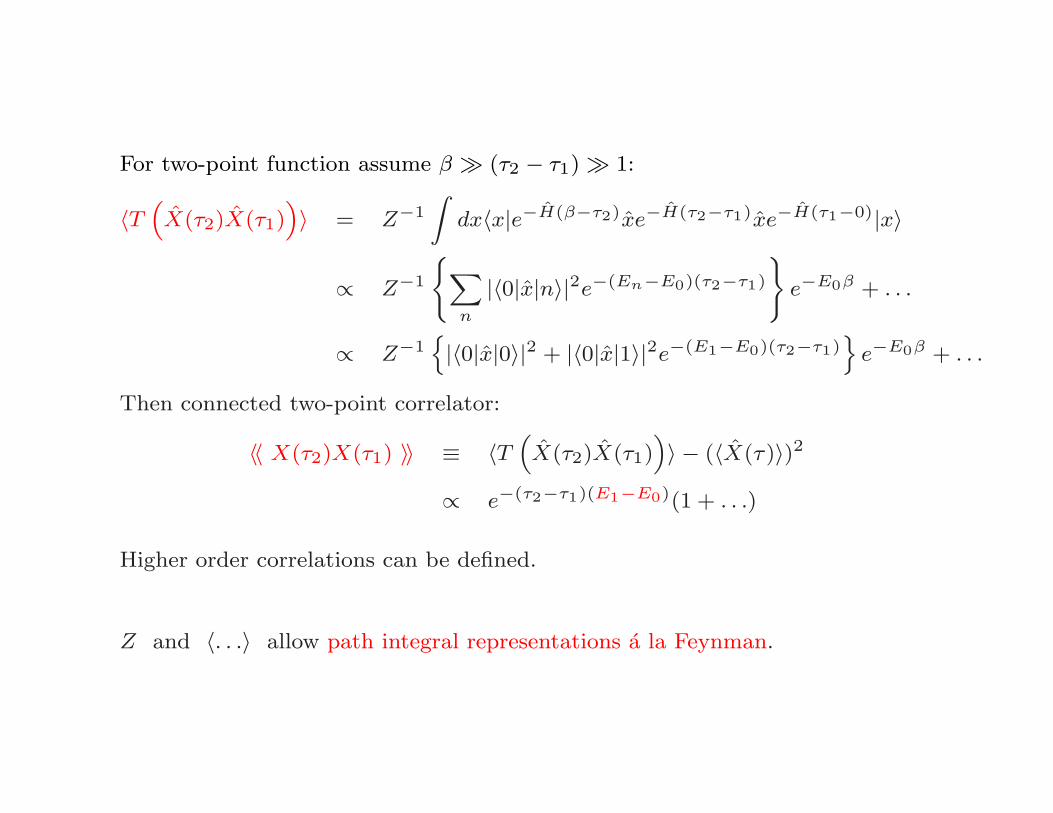
For two-point function assume β ≫ (τ2 − τ1) ≫ 1:

〈T(

X(τ2)X(τ1))

〉 = Z−1

∫

dx〈x|e−H(β−τ2)xe−H(τ2−τ1)xe−H(τ1−0)|x〉

∝ Z−1

∑

n

|〈0|x|n〉|2e−(En−E0)(τ2−τ1)

e−E0β + . . .

∝ Z−1

|〈0|x|0〉|2 + |〈0|x|1〉|2e−(E1−E0)(τ2−τ1)

e−E0β + . . .

Then connected two-point correlator:

〈〈 X(τ2)X(τ1) 〉〉 ≡ 〈T(

X(τ2)X(τ1))

〉 − (〈X(τ)〉)2

∝ e−(τ2−τ1)(E1−E0)(1 + . . .)

Higher order correlations can be defined.

Z and 〈. . .〉 allow path integral representations a la Feynman.

Path integral representation

Subdivide β = Nǫ = fix with N → ∞ , ǫ→ 0 .

Use (N − 1) times completeness relation∫

dx |x〉〈x| = 1.

Z =

∫ N∏

i=1

dxi 〈xN |e−Hǫ|xN−1〉 · 〈xN−1|e−Hǫ|xN−2〉 · · · 〈x1|e−Hǫ|x0〉

with x0 ≡ xN , i.e. “periodic boundary condition”.

For one degree of freedom: H = T + V = p2/2m+ V (x) , [x, p] = i

Transfer matrix : 〈x′|e−Hǫ|x〉 =√

ǫ

2πe−

12ǫ

(x′−x)2− ǫ2[V (x)+V (x′)] +O(ǫ3) ,

=⇒ Z ∼∫

Dx(τ) e−SE [x(τ)]

Proof applies Trotter product formula:

exp(−βH) ≡ exp(−(T + V )ǫ)N = limN→∞

(

exp(−ǫT ) · exp(−ǫV ))N

Dx(τ) ≡ limN→∞

( ǫ

2π

)N/2N∏

i=1

dxi, SE [x(τ)] ∼∫

dτ

[

m

2

(

dx(τ)

dτ

)2

+ V (x(τ))

]

.

Result: summation over fictitious paths in imaginary time

n

x

1

xn

n−1

3

2

1τ

τ

τ

τ

τ

Our main interest: correlation functions in Heisenberg picture:

〈 Ω(τ ′, τ ′′, ...) 〉 = Z−1

∫

Dx(τ) Ω(τ ′, τ ′′, ...) e−SE [x(τ)] .

(Proof as for partition function Z.)

=⇒ no operators, but trajectories x(τ) and Euclidean action SE [x(τ)],

=⇒ correlators resemble classical statistical averages,

=⇒ we use β = Nǫ with N finite, but large, i.e. “lattice approximation”.

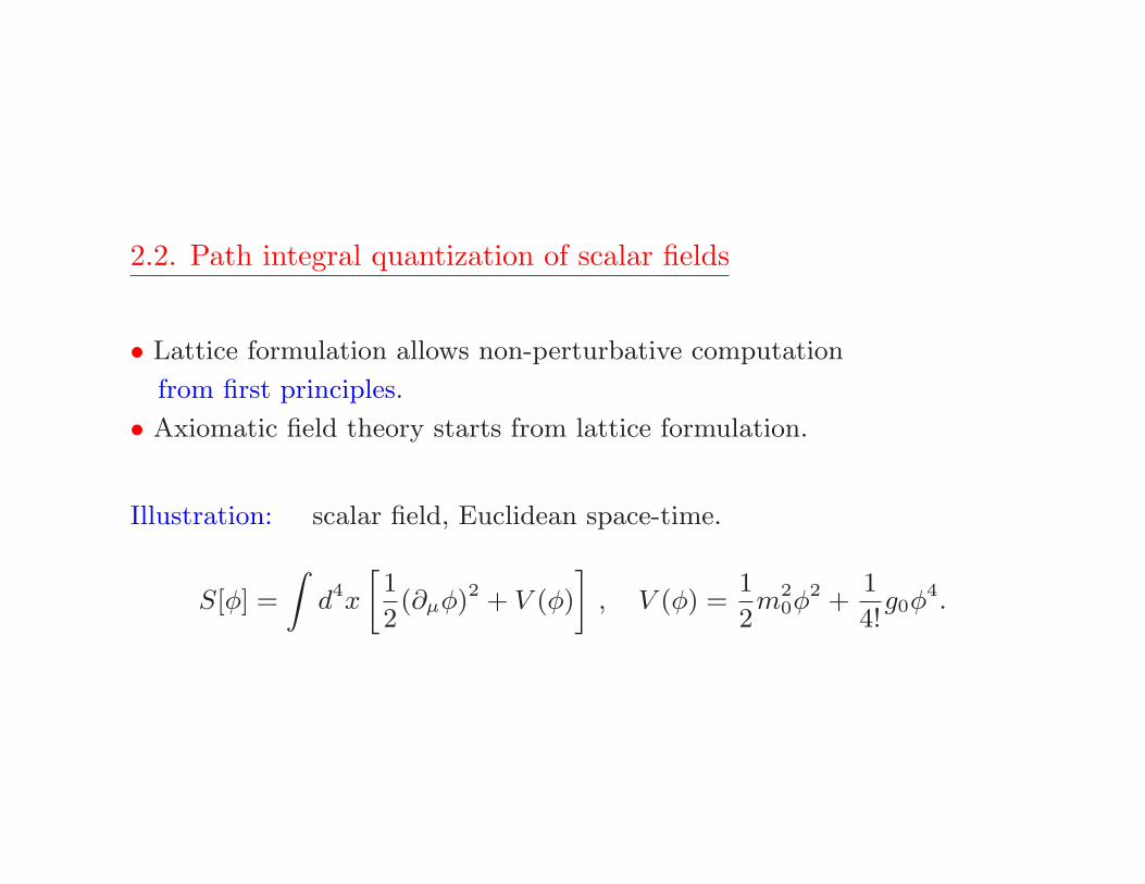
2.2. Path integral quantization of scalar fields

• Lattice formulation allows non-perturbative computation

from first principles.

• Axiomatic field theory starts from lattice formulation.

Illustration: scalar field, Euclidean space-time.

S[φ] =

∫

d4x

[

1

2(∂µφ)

2 + V (φ)

]

, V (φ) =1

2m2

0φ2 +

1

4!g0φ

4.

a

L = NSa

L 4 = N

4ax −→ xn

φ(x) −→ φn ≡ φ(xn)

∂µφ(x) −→ 1a(φn+µ − φn)

[“Lattice” taken from A. Kronfeld, hep-ph/0209231]

SLatt = a4∑

n

1

2

4∑

µ=1

(φn+µ − φn)2 1

a2+ V (φn)

=⇒ no unique discretization,

=⇒ even more - systematic improvement scheme exists (Symanzik).

Boundary condition: φ(x+ Lµ · µ) = φ(x)

Spectrum: −πa≤ kµ = 2π

Lµnµ ≤ π

a

Quantization:

Path integral for time ordered correlation functions and vacuum

transition amplitude

< φ(x1 · · ·φ(xN ) > = Z−1

∫

∏

x

dφ(x)φ(x1) · · ·φ(xN )e−S[φ] (1)

Z =

∫

∏

x

dφ(x) e−S[φ] (2)

m lattice approximation and rescaling φ −→ φ · √g0 .

< φn1 · · ·φnN > = Z−1Latt

∫

∏

n

dφnφn1 · · ·φnN e−1g0SLatt (3)

ZLatt =

∫

∏

n

dφn e− 1

g0SLatt (4)

Compare with: Z(T, V ) =∫∏fi=1 dqi dpi e

− 1kT

H(qi,pi)

Scalar Higgs model in some detail:

φ =√2κ

ϕ

a, g0 =

6λ

κ2, m2

0 =1− 2λ− 8κ

a2κ.

SLatt = −2κ∑

n,µ

ϕnϕn+µ + λ∑

n

(ϕ2n − 1)2 +

∑

n

ϕ2n

(κ ‘Hopping parameter’)

No lattice spacing visible. How does the continuum limit occur?

In practice need for determining correlation lengths

L4 = N4a ≫ ζ ≡ m−1 ≫ a

Continuum limit corresponds to 2nd order phase transition:

ζ/a → ∞ whereas m1/m2 → const.

λ → ∞ : κ = fixed =⇒ ϕn = ±1 .

ZLatt → const. ·∑

ϕn=±1

exp

(

−2κ∑

n,µ

ϕnϕn+µ

)

=⇒ Ising model in 4D,

=⇒ 2nd order phase transition at κc = 0.0748.

λ < ∞ : find critical line κ = κc(λ).

Comment:

renormalized coupling λren → 0 for κ → κc

=⇒ non-interacting theory in the continuum limit or

=⇒ effective theory at finite cutoff.

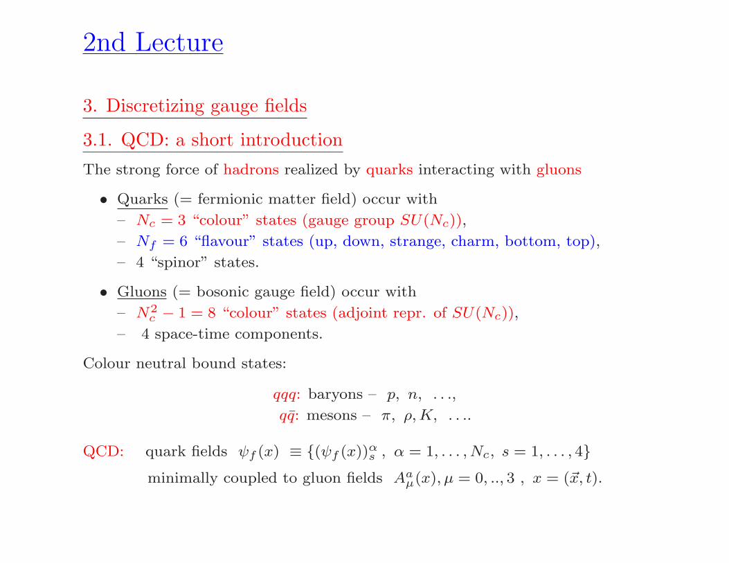
2nd Lecture

3. Discretizing gauge fields

3.1. QCD: a short introduction

The strong force of hadrons realized by quarks interacting with gluons

• Quarks (= fermionic matter field) occur with

– Nc = 3 “colour” states (gauge group SU(Nc)),

– Nf = 6 “flavour” states (up, down, strange, charm, bottom, top),

– 4 “spinor” states.

• Gluons (= bosonic gauge field) occur with

– N2c − 1 = 8 “colour” states (adjoint repr. of SU(Nc)),

– 4 space-time components.

Colour neutral bound states:

qqq: baryons – p, n, . . .,

qq: mesons – π, ρ,K, . . ..

QCD: quark fields ψf (x) ≡ (ψf (x))αs , α = 1, . . . , Nc, s = 1, . . . , 4minimally coupled to gluon fields Aaµ(x), µ = 0, .., 3 , x = (~x, t).

S[ψ, ψ,A] =

∫

d4x

−1

2tr GµνGµν +

Nf∑

f=1

ψf (iγµDµ −mf )ψf

Gµν = ∂µAν − ∂νAµ + ig0[Aµ, Aν ] , Dµ = ∂µ1+ ig0Aµ , Aµ = AaµTa ,

Ta (a = 1, . . . , N2c − 1) – generators of SU(Nc),

with [Ta, T b] = ifabcT c, 2tr(TaT b) = δab, trTa = 0.

• local gauge invariance – the main principle of the standard model

ψ′(x) = g(x)ψ(x), A′µ(x) = g(x)Aµg

†(x)− i

g0(∂µg(x))g

†(x), g(x) ∈ SU(Nc)

leaves action S[ψ, ψ,A] invariant for any g(x).

• quantization with Euclidean path integral analogously to QM:

〈 Ω(ψ, ψ,A) 〉 = Z−1

∫

DAµDψDψ Ω(ψ, ψ,A) e−SE [ψ,ψ,A]

DAµ =∏

x

dAµ(x) ; Dψ =∏

x

dψ(x) − Grassmannian measure

=⇒ weak coupling (αs ≪ O(1)): perturbation theory, requires gauge fixing;

=⇒ stronger coupling (αs ≃ O(1)): lattice theory, Dyson-Schwinger eqs., ...

3.2. Gauge fields on a lattice

K. Wilson ’74:

Local SU(Nc) gauge symmetry kept exact by non-local prescription

on a 4d Euclidean lattice =⇒ link variables

Aµ(xn) =⇒ Un,µ ≡ P exp ig0

∫ xn+µa

xn

Aµ(x)dxµ ∈ SU(Nc)

≃ eiag0Aµ(xn) ≃ 1+ iag0Aµ(xn) +O(a2)

Gauge transformation gn ≡ g(xn) ∈ SU(Nc) for a→ 0:

A′µ(xn) ≃ gnAµg

†n − i

ag0(gn+µ − gn)g

†n

U ′n,µ = 1+ iag0A

′µ(xn) +O(a2)

= iag0 gnAµg†n + gn+µg

†n +O(a2), gn = gn+µ +O(a)

= gn+µ(1+ iag0Aµ(xn) +O(a2))g†n

= gn+µ Un,µ g†n

Transformation of a product of variables of connected links

U ′(n+ µ+ ν, n) ≡ U ′n+µ,νU

′n,µ = gn+µ+νUn+µ,νUn,µg

†n = gn+µ+νU(n+ µ+ ν, n)g†n

can be generalized to arbitrary continuum path:

“Schwinger line” (parallel transporter)

U(x2, x1) = P exp

ig0

∫ x2

x1

Aµdxµ

,

=⇒ U ′(x2, x1) = g(x2)U(x2, x1)g†(x1).

=⇒ tr

(

P exp

ig0

∮

Aµdxµ

)

= invariant.

Combination with matter field: ψ′(x) = g(x)ψ(x), ψ′†(x) = ψ†(x)g†(x)

=⇒ ψ†(x2)U(x2, x1)ψ(x1) = invariant.

Lattice gauge action: from elementary closed (Wilson) loops (“plaquettes”)

Un,µν ≡ Un Un+µ,ν U†n+ν,µ U

†n,ν ,

SWG = β∑

n,µ<ν

(

1 − 1

NcRe tr Un,µν

)

, β =2Nc

g20

=1

2

∑

n

a4 tr GµνGµν +O(a2),

→ 1

2

∫

d4x tr GµνGµν .

Homework I:

Prove the continuum limit in the (non-) Abelian case: −→ tutorial.

Comments:

- Improvement of SWG : suppression of O(a)-corrections

by adding contributions from larger loops (e.g. various 6-link loops)

or contributions of loops in higher group representations (e.g. adjoint

representation)

- Useful test for programmers: non-trivial vacuum field = pure gauge

U(vac)nµ ≡ gn+µ g

†n, for arbitrary gn ∈ SU(Nc)

Re tr Un,µν = Nc =⇒ SWG = 0.

Path integral quantization:

replacement∫ ∏

x,µ dAµ(x) −→∫ ∏

n,µ[dU ]n,µ, [dU ] “Haar measure”.

Properties: U, V ∈ G = SU(Nc) in fundamental representation, then

•∫

G[dU ] = 1 normalization,

•∫

Gf(U)[dU ] =

∫

Gf(V U)[dU ] =

∫

Gf(UV )[dU ], [d(UV )] = [d(V U)] = [dU ],

•∫

Gf(U)[dU ] =

∫

Gf(U−1)[dU ] .

Examples:

U(1) : U = eiϕ =⇒ [dU ] = 12π dϕ,

∫

f(U)[dU ] ≡ 12π

∫ 2π0

dϕ f(U(ϕ));

SU(2) : U = B0 + i~σ · ~B,∑

i(Bi)2 = 1 =⇒ [dU ] = 1

π2 δ(B2 − 1) d4B,

~σ – Pauli matrices.

Expectation values, correlation functions in pure gauge theory:

〈W 〉 = 1

Z

∫

(∏

n,µ

[dUnµ]) W [U ] e−SG[U ], Z =

∫

(∏

n,µ

[dUnµ]) e−SG[U ] .

Gauge invariance:

U ′nµ = gn+µ Unµg

†n =⇒ dU ′

nµ = dUnµ, SG[U′] = SG[U ]

Then immediately

〈W ′〉 =1

Z′

∫

(∏

n,µ

[dU ′nµ]) W [U ′] e−SG[U′]

=1

Z

∫

(∏

n,µ

[dUnµ]) W [U ′] e−SG[U ]

=⇒ invariant, if W [U ] itself is gauge invariant.

Fortunately, holds in most of the applications of lattice gauge theory !

Exceptions:

Quark, gluon, ghost propagators or various vertex functions.

Gauge fixing is required, e.g. Landau/Lorenz gauge, as in perturbation theory.

However, gauge condition not uniquely solvable - “Gribov problem”.

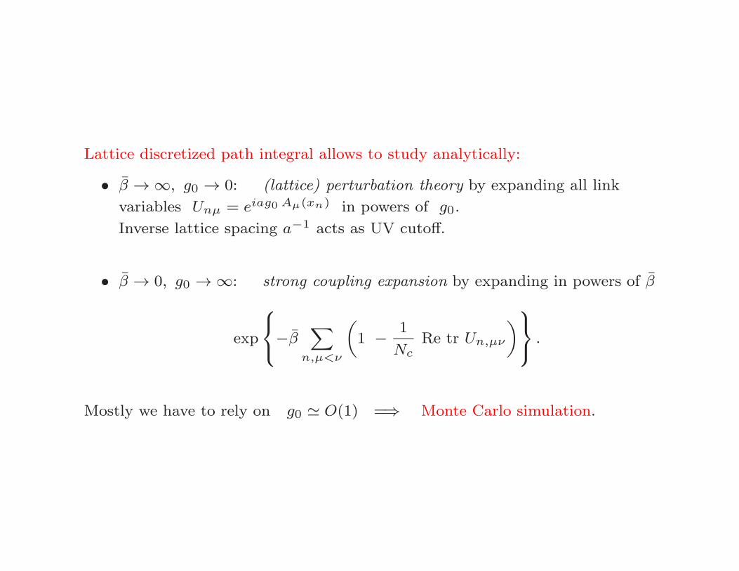
Lattice discretized path integral allows to study analytically:

• β → ∞, g0 → 0: (lattice) perturbation theory by expanding all link

variables Unµ = eiag0 Aµ(xn) in powers of g0.

Inverse lattice spacing a−1 acts as UV cutoff.

• β → 0, g0 → ∞: strong coupling expansion by expanding in powers of β

exp

−β∑

n,µ<ν

(

1 − 1

NcRe tr Un,µν

)

.

Mostly we have to rely on g0 ≃ O(1) =⇒ Monte Carlo simulation.

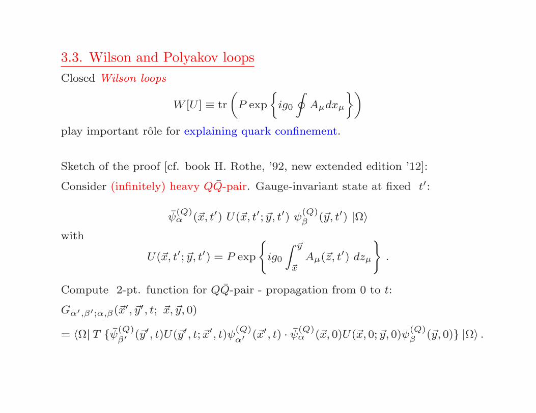
3.3. Wilson and Polyakov loops

Closed Wilson loops

W [U ] ≡ tr

(

P exp

ig0

∮

Aµdxµ

)

play important role for explaining quark confinement.

Sketch of the proof [cf. book H. Rothe, ’92, new extended edition ’12]:

Consider (infinitely) heavy QQ-pair. Gauge-invariant state at fixed t′:

ψ(Q)α (~x, t′) U(~x, t′; ~y, t′) ψ

(Q)β (~y, t′) |Ω〉

with

U(~x, t′; ~y, t′) = P exp

ig0

∫ ~y

~xAµ(~z, t

′) dzµ

.

Compute 2-pt. function for QQ-pair - propagation from 0 to t:

Gα′,β′;α,β(~x′, ~y′, t; ~x, ~y, 0)

= 〈Ω| T ψ(Q)β′ (~y′, t)U(~y′, t; ~x′, t)ψ

(Q)α′ (~x′, t) · ψ(Q)

α (~x, 0)U(~x, 0; ~y, 0)ψ(Q)β (~y, 0) |Ω〉 .

Euclidean time t = −iτ ; for τ → ∞, MQ → ∞ expect

Gα′,β′;α,β ∝ δ(3)(~x− ~x′) δ(3)(~y − ~y′) Cα′,β′;α,β(~x, ~y) exp(−E(R)τ)

E(R) = energy of the lowest state (above vacuum), i.e. QQ-potential.

Path integral representation:

Gα′,β′;α,β =1

Z

∫

DA

∫

Dψ(Q)

Dψ(Q)

(

ψ(Q)

β′ (~y′, τ) . . . ψ

(Q)β (~y, 0)

)

exp(−S[ψ(Q)

, ψ(Q)

, A])

Carry out (Grassmanian) fermion integration

−→ product of Green’s functions for Q, Q and Det → const for MQ → ∞.

Static limit – neglect spatial derivatives (iγµDµ) → (iγ4D4)

−→ Green’s function:

[iγ4D4(A)−MQ] K(z, z′;A) = δ(4)(z − z′).

Solution:

K(z, z′;A) ∼ P exp

ig0

∫ τ

0A0(~z, t

′) dt′

δ(3)(~z − ~z′) ·K

with K containing projectors P± = 12(1± γ4).

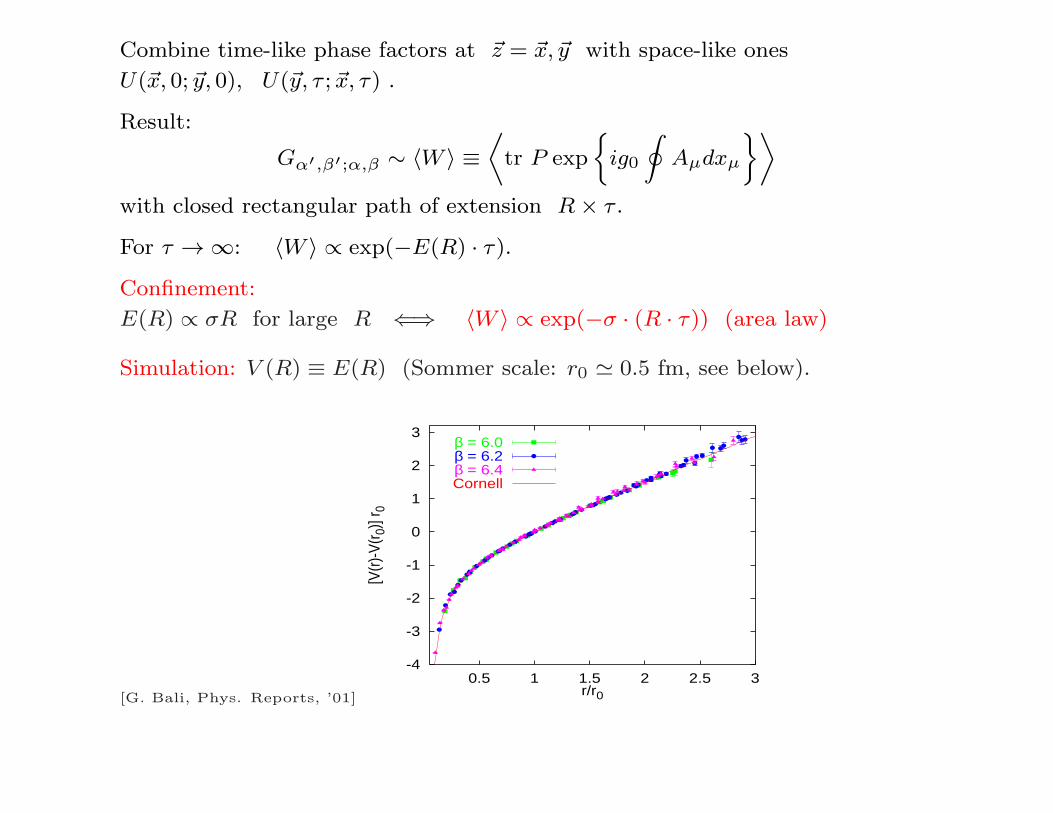
Combine time-like phase factors at ~z = ~x, ~y with space-like ones

U(~x, 0; ~y, 0), U(~y, τ ; ~x, τ) .

Result:

Gα′,β′;α,β ∼ 〈W 〉 ≡⟨

tr P exp

ig0

∮

Aµdxµ

⟩

with closed rectangular path of extension R× τ .

For τ → ∞: 〈W 〉 ∝ exp(−E(R) · τ).

Confinement:

E(R) ∝ σR for large R ⇐⇒ 〈W 〉 ∝ exp(−σ · (R · τ)) (area law)

Simulation: V (R) ≡ E(R) (Sommer scale: r0 ≃ 0.5 fm, see below).

[G. Bali, Phys. Reports, ’01]

-4

-3

-2

-1

0

1

2

3

0.5 1 1.5 2 2.5 3

[V(r

)-V

(r0)

] r0

r/r0

β = 6.0β = 6.2β = 6.4Cornell

Polyakov loops and non-zero temperature QCD [cf. lecture by O. Philipsen]

[Gross, Pisarski, Yaffe, Rev.Mod.Phys. 53 (1981) 43;

Svetitsky, Yaffe, Nucl.Phys. B210 (1982) 423; Svetitsky, Phys.Rept. 132 (1986) 1]

Partition function:

Z = Tr exp(−βH), β = 1/kBT,

=∑

x

〈x|(exp(−ǫH))N |x〉, Nǫ = β,

= C

∫

Dx exp(−SE [x(t)]), SE =

∫ β

0dt [

m

2x(t)2 + V (x(t))]

with x(0) = x(β), i.e. periodicity.

For Yang-Mills theory analogous proof of path integral representation is

non-trivial:

– Hamiltonian approach within gauge Aa0 = 0,

– trace integration produces integration over auxiliary field Aa4 ,

=⇒ full Euclidean Yang-Mills action recovered.

Result:

ZG = C

∫

DAe−SG[A], SG[A] =

∫ β

0dt

∫

d3x1

2tr(GµνGµν)

with Aaµ(~x, 0) = Aaµ(~x, β), and Gµν = GaµνTa Euclidean.

Applied to lattice pure gauge theory:

ZG ≡∫

[dU ]e−SG[U ], with Uµ(~x, 0) = Uµ(~x, β), β = aN4 =1

kBT.

We are interested in the thermodynamic limit: V (3) → ∞.

In practice, “aspect ratio” Ns/N4 ≫ 1 and periodic b.c.’s in spatial directions.

Extension to full QCD: time-antiperiodic boundary conditions for fermionic

fields from trace of statist. operator: ψ(~x, 0) = −ψ(~x, β), ψ(~x, 0) = −ψ(~x, β).Polyakov loop:

L(~x) ≡ 1

Nctr

N4∏

x4=1

U4(~x, x4), (a = 1),

invariant w.r. to time-periodic gauge transformations g(~x, 1) = g(~x,N4 + 1).

Physical interpretation:

〈L(~x)〉 = exp(−βFQ),

with FQ free energy of an isolated infinitely heavy quark.

Proof goes analogously as for Wilson loop expectation value.

=⇒ FQ → ∞, i.e. 〈L(~x)〉 → 0 within the confinement phase.

=⇒ 〈L(~x)〉 order parameter for the deconfinement transition.

Spontaneous breaking of ZN center symmetry:

zν = e2πiνN 1 ∈ ZN ⊂ SU(N), ν = 0, 1, . . . , N − 1

commute with all elements of SU(N). For SU(2): zν = ±1.

Global ZN -transformation:

U4(~x, x4) → z · U4(~x, x4) for all ~x and fixed x4

=⇒ L(~x) → zL(~x) not invariant.

=⇒ Plaquette values Un,i4 → zz⋆Un,i4 = Un,i4 , i.e. SG invariant.

SU(2)-case:

L(~x) → −L(~x) . Both states have same statistical weight.

=⇒ 〈L(~x)〉 = 0 .

=⇒ Order parameter for the deconfinement transition:

〈|L|〉 ≡⟨

| 1

V (3)

∑

~x

L(~x)|⟩

∼

0 confinement

1 deconfinement

analogously to spin magnetization for 3d Ising model.

SU(3)-case: L complex-valued.

Confinement → L ≃ 0,

Deconfinement → L ≃ zν , ν = 0, 1, 2.

Notice: fermions break center symmetry. Then

⇒ Polyakov loop – order parameter for (de)confinement only if mq → ∞,

⇒ quark condensate 〈ψψ〉 – strict order parameter

for chiral symmetry breaking / restoration only if mq → 0.

3.4. Fixing the QCD scale

Expectation values 〈W 〉 (of Wilson loops etc.) in pure gauge theory only

depend on parameter β ≡ 2Nc/g20 (and linear lattice extensions Nµ).

View some Monte Carlo results in gluodynamics.

0 0.2 0.4 0.6 0.8 r [fm]

−0.5

0

0.5

V(r) [GeV]

perturbation theory

Static QQ potential V (r) (≡ E(R)) at small distances from Wilson loops.

Necco, Sommer, ’02

Alternative method: Polyakov loop correlator

〈L( ~x1L( ~x2†)〉 ∝ exp(−βV (r))(1 + . . .), r ≡ | ~x1 − ~x2|

0 2 4 6 (r [fm])-21

1.1

1.2

1.3

1.4

1.5

V //(r) [GeV/fm]

1.0 fm 0.5 fm

σ

Static QQ force F (r) ≡ dV/dr from Polyakov loop correlators at T = 0.

=⇒ in perfect agreement with string model prediction

V (r) ∼ σr + µ− π

12 r+O(r−2).

Luscher, Weisz, ’02

F (r) allows to fix the scale by comparing with phenomenologically known cc-

or bb-potential [R. Sommer, ’94]:

F (r0) r20 = 1.65 ↔ r0 ≃ 0.5 fm

If Sommer scale r0 is determined in lattice units a for certain β, spacing

a(β) can be fixed in physical units.

3.5. Renormalization group and continuum limit

Assume for a physical observable Ω (e.g. string tension σ, critical temperature

Tc, glueball mass Mg , . . .) in the continuum limit

lima→0

Ω (g0(a), a) = Ωc

Then renormalization group Eq.

d Ω

d(ln a)= 0 =⇒

(

∂

∂(ln a)− β(g0)

∂

∂g0

)

Ω (g0, a) = 0

with β(g0) ≡ − ∂ g0∂(ln a)

known from perturbation theory

β(g)/g3 = −β0 − β1g2 +O(g4).

For SU(Nc) and Nf massless fermions, independent on renormalization scheme:

β0 =1

(4π)2

(

11

3Nc −

2

3Nf

)

,

β1 =1

(4π)4

(

34

3N2c − 10

3NcNf − N2

c − 1

NcNf

)

.

For pure gluodynamics: Nc = 3, Nf = 0 ⇒ β0 > 0.

Solution yields continuum limit

a(g0) =1

ΛLatt(β0g

20)

−β12β2

0 exp

(

− 1

2β0g20

)

(1 +O(g20)).

=⇒ 1/a→ ∞ for g0 → 0 (or β → ∞), asymptotic freedom.

Corresponds to second order phase transition.

In practice, tune g0, N4 for getting correlation lengths ξ, such that:

N4 ≫ ξ/a(g0) ≫ 1 .

At non-zero T = 1/L4 = 1/(N4a(β)) :

T can be varied by changing β at fixed N4 or N4 at fixed β.

3rd Lecture

4. Simulating gauge fields

4.1. How does Monte Carlo work?

Realization in quantum mechanics:

M. Creutz, B. Freedman, A stat. approach to quantum mechanics, Annals Phys. 132(1981)427

Here consider n-dim. integral:

〈f〉 =∫

Ω dnx f(x)w(x) with 0 ≤ w(x) ≤ 1,

∫

Ω w(x) dnx = 1.

〈f〉 =∫

Ωdnx f(x)

∫ w(x)

0dη =

∫

Ωdnx

∫ 1

0dη f(x)Θ(w(x)− η)

Importance sampling by selecting x in acc. with w(x):

(a) choose randomly: x ∈ Ω and η ∈ [0, 1],

(b) acceptance check: accept x, if η satisfies η < w(x), otherwise reject.

=⇒ From accepted x(i)’s estimate 〈f〉 ≃ (1/N)∑Ni=1 f(x

(i)).

=⇒ However, efficiency small, if acceptance rate in large areas of Ω is low.

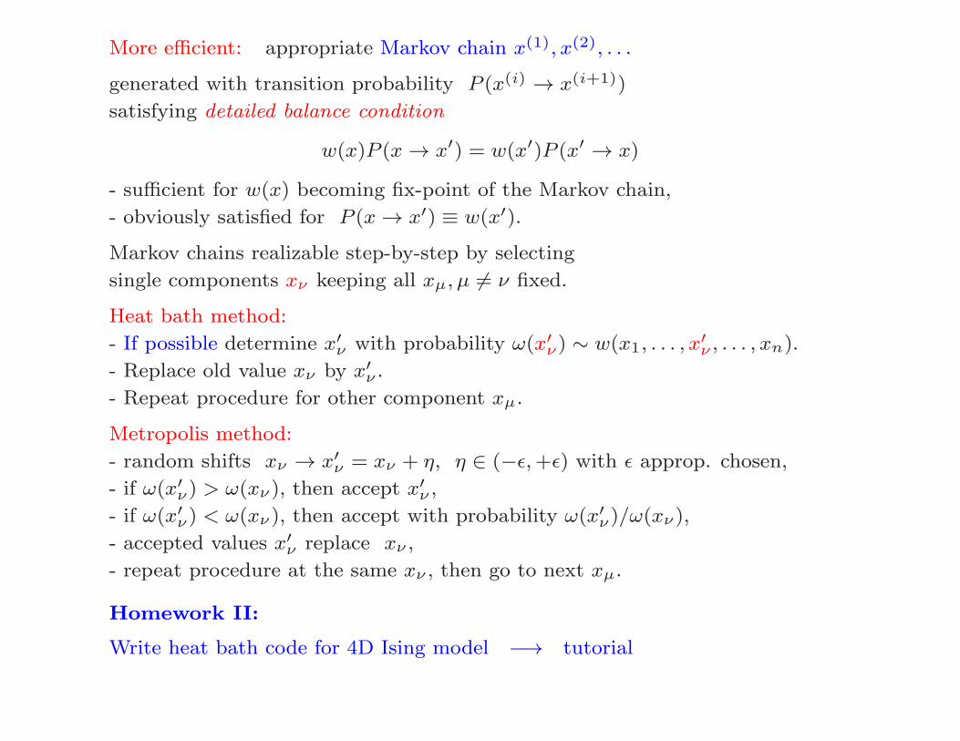
More efficient: appropriate Markov chain x(1), x(2), . . .

generated with transition probability P (x(i) → x(i+1))

satisfying detailed balance condition

w(x)P (x→ x′) = w(x′)P (x′ → x)

- sufficient for w(x) becoming fix-point of the Markov chain,

- obviously satisfied for P (x→ x′) ≡ w(x′).

Markov chains realizable step-by-step by selecting

single components xν keeping all xµ, µ 6= ν fixed.

Heat bath method:

- If possible determine x′ν with probability ω(x′ν) ∼ w(x1, . . . , x′ν , . . . , xn).

- Replace old value xν by x′ν .

- Repeat procedure for other component xµ.

Metropolis method:

- random shifts xν → x′ν = xν + η, η ∈ (−ǫ,+ǫ) with ǫ approp. chosen,

- if ω(x′ν) > ω(xν), then accept x′ν ,

- if ω(x′ν) < ω(xν), then accept with probability ω(x′ν)/ω(xν),

- accepted values x′ν replace xν ,

- repeat procedure at the same xν , then go to next xµ.

Homework II:

Write heat bath code for 4D Ising model −→ tutorial

4.2. Creutz’ heat bath method

Assume statistical weight w[U ] ∼ e−SG[U ] with plaquette action

SG[U ] = β∑

n,µ<ν

(

1 − 1

NcRe tr Un,µν

)

.

Select a single link variable: Un0,µ0 ≡ U0. There are 6 plaquettes containing

this link and contributing to SG:

SG[U0; U \ U0] = C[U \ U0]−β

Nc

6∑

S=1

Re tr (U0US)

= C − β

NcRe tr (U0A), A =

6∑

S=1

US

Call open plaquette US = “staple”.

Assume A be fixed (“heat bath”) =⇒ link variable U0 to be determined with

probability

w(U0) [dU0] ∼ exp

(

β

NcRe tr (U0A)

)

[dU0]

.

Metropolis:

- apply random shifts U0 → U ′0 = GU0, with G ∈ Uǫ(1) ⊂ SU(Nc),

- carry out Metropolis acceptance steps.

Heat bath for SU(2):

Normalize V = A/√detA ∈ SU(2), put V U0 ≡ U and use invariance of Haar

measure

w(U)[dU ] ∼ exp (ρ tr U) [dU ], ρ =β√detA

2

U ≡ B01+ i~σ ~B, [dU ] =1

π2δ(B2 − 1) d4B, tr U = 2B0

=⇒ w(U)[dU ] ∼ exp(

2ρB0)

δ(B2 − 1) d4B

=⇒ determine U and U0 = V †U .

Heat bath for SU(Nc) [Cabibbo, Marinari, ’82]

Use SU(2) heat bath algorithm for various subgroup embeddings into SU(Nc).

5. Fermions on the lattice

5.1. Naive discretization and fermion doubling

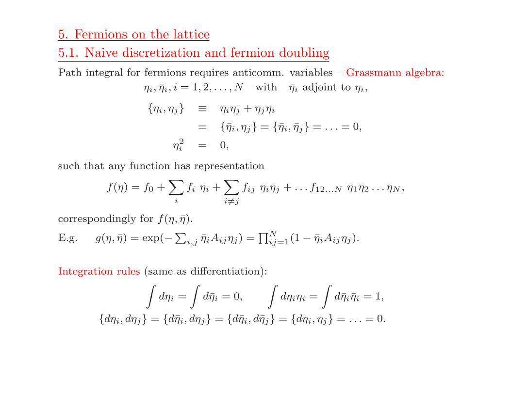
Path integral for fermions requires anticomm. variables – Grassmann algebra:

ηi, ηi, i = 1, 2, . . . , N with ηi adjoint to ηi,

ηi, ηj ≡ ηiηj + ηjηi

= ηi, ηj = ηi, ηj = . . . = 0,

η2i = 0,

such that any function has representation

f(η) = f0 +∑

i

fi ηi +∑

i 6=j

fij ηiηj + . . . f12...N η1η2 . . . ηN ,

correspondingly for f(η, η).

E.g. g(η, η) = exp(−∑i,j ηiAijηj) =∏Nij=1(1− ηiAijηj).

Integration rules (same as differentiation):∫

dηi =

∫

dηi = 0,

∫

dηiηi =

∫

dηiηi = 1,

dηi, dηj = dηi, dηj = dηi, dηj = dηi, ηj = . . . = 0.

Most important for us:

I[A] =

∫ N∏

l=1

dηldηl exp

−N∑

ij=1

ηiAijηj

= detA,

Z[A; ρ, ρ] =

∫ N∏

l=1

dηldηl exp

−N∑

ij=1

ηiAijηj +∑

i

(ηiρi + ρiηi)

,

= detA · exp

N∑

ij=1

ρiA−1ij ρj

,

〈ηiηj〉 =

∫

DηDη ηiηj exp(−ηAη)∫

DηDη exp(−ηAη) = A−1ij .

Dirac Propagator (with Euclidean: γµ, γν = 2δµν , γ4 ≡ γ0M , γi ≡ −iγiM )

〈ψα(x)ψβ(y)〉 =

∫

DψDψ ψα(x)ψβ(y) exp(

−SF [ψψ]

)∫

DψDψ exp(

−SF [ψψ]) ,

SF [ψψ] =

∫

d4x ψ(x)(γµ∂µ +m)ψ(x).

Naive lattice discretization:

rescale m→M/a, ψα(xn) → 1a3/2

ψα(n), ∂µψα(xn) → 1a5/2

∂µψα(n)

∂µψα(n) =1

2[ψα(n+ µ)− ψα(n− µ)]

SF [ψψ] ≃∑

n,m;α,β

ψα(n)Kαβ(n,m)ψβ(m)

with Kαβ(n,m) = 12

∑

µ(γµ)αβ [δm,n+µ − δm,n−µ] +M δmnδαβ

Free lattice Dirac propagator:

〈ψα(x)ψβ(y)〉 = lima→0

∫ π/a

−π/a

d4p

(2π)4

[−i∑

µ γµpµ +m]αβ∑

µ p2µ +m2

eip(x−y)

with pµ = 1asin(pµa) to be compared with scalar case kµ = 2

asin(kµa/2).

For M = 0 in momentum space we get poles at all 2d corners of the Brillouin

zone [(0000), (π/a 000), . . .]. =⇒ “Doubling of fermion degrees of freedom”.

Homework III:

Determine lattice propagator for free scalar field −→ tutorial

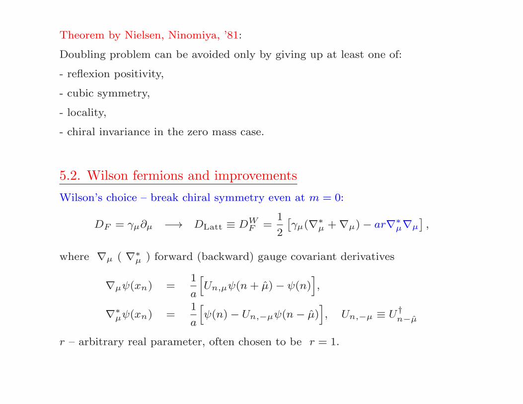
Theorem by Nielsen, Ninomiya, ’81:

Doubling problem can be avoided only by giving up at least one of:

- reflexion positivity,

- cubic symmetry,

- locality,

- chiral invariance in the zero mass case.

5.2. Wilson fermions and improvements

Wilson’s choice – break chiral symmetry even at m = 0:

DF = γµ∂µ −→ DLatt ≡ DWF =1

2

[

γµ(∇∗µ +∇µ)− ar∇∗

µ∇µ]

,

where ∇µ ( ∇∗µ ) forward (backward) gauge covariant derivatives

∇µψ(xn) =1

a

[

Un,µψ(n+ µ)− ψ(n)]

,

∇∗µψ(xn) =

1

a

[

ψ(n)− Un,−µψ(n− µ)]

, Un,−µ ≡ U†n−µ

r – arbitrary real parameter, often chosen to be r = 1.

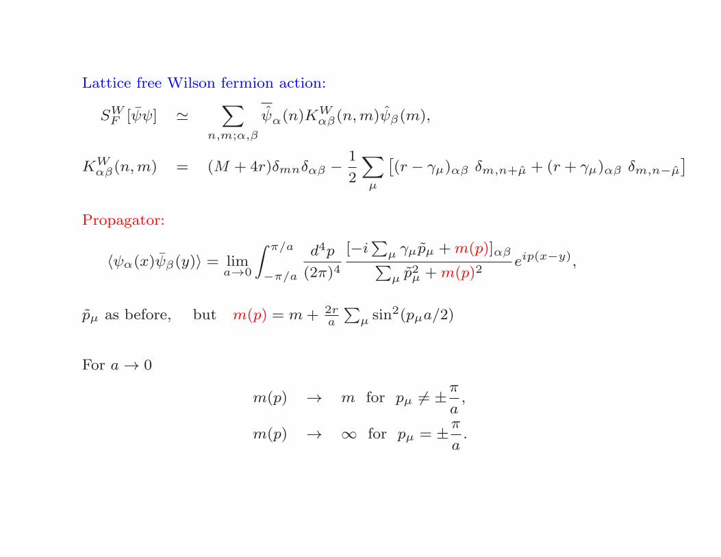
Lattice free Wilson fermion action:

SWF [ψψ] ≃∑

n,m;α,β

ψα(n)KWαβ(n,m)ψβ(m),

KWαβ(n,m) = (M + 4r)δmnδαβ − 1

2

∑

µ

[

(r − γµ)αβ δm,n+µ + (r + γµ)αβ δm,n−µ]

Propagator:

〈ψα(x)ψβ(y)〉 = lima→0

∫ π/a

−π/a

d4p

(2π)4

[−i∑

µ γµpµ +m(p)]αβ∑

µ p2µ +m(p)2

eip(x−y),

pµ as before, but m(p) = m+ 2ra

∑

µ sin2(pµa/2)

For a→ 0

m(p) → m for pµ 6= ±πa,

m(p) → ∞ for pµ = ±πa.

Problems:

• Chiral SU(3)A flavor symmetry explicitly broken.

• Eigenvalue value spectrum of DWF strongly differs from continuum

spectrum.

• Discretization error δSWF ∼ O(a) compared with δSWG ∼ O(a2)

=⇒ improvement possible with clover term

ScloverF = SWF + a5∑

n

cswψ(xn)i

4σµν Fµνψ(xn) .

Sheikholeslami, Wohlert ’85

=⇒ alternative: twisted-mass fermions at maximal twist (cf. K. Jansen).

Chiral improvement: Ginsparg-Wilson fermions

Any lattice Dirac operator satisfying the Ginsparg-Wilson relation (GWR)

Ginsparg, Wilson ’82

γ5DLatt +DLattγ5 = aDLattγ5DLatt

guaranties approximately local ( ∼ O(a)), but exact chiral symmetry.

Luscher ’98

Strategies to solve GWR:

• Neuberger’s operator: exact solution of GWR

D +m → DN =

1 +m

2(1 + A (A†A)−

12 )

, A = 1 + s−DWF

Neuberger ’98

Properties:

– (√A†A)−1 numerically involved:

approximation by polynomials (Chebyshev approx.).

– Det DN hard to compute, but required for full fermionic simulation.

– Discretization error still O(a2).

• Equivalent alternative domain wall fermions: extension to 5 dimensions

DLatt =1

2[γ5(∂

∗s + ∂s)− as∂

∗s∂s] +DWF − ρ

a, 0 < ρ < 2

with boundary condition

P+ψ( o, x) = P−ψ( (Ns + 1) as, x) = 0 , P± = (1± γ5)/2

and limit Ns → ∞ and as → 0

Kaplan ’92; Shamir ’93

• Approximative methods:

– Renormalization group based perfect action approach

P. Hasenfratz, Niedermayer ’94; DeGrand, ... ’94

– generalized (less local) ansatzes for DLatt with parameters fixed from

GWR

Gattringer ’01

5.3. Staggered fermions

Kogut, Susskind, ’75

• Use naive discretization and diagonalize action w.r. to spinor degrees of

freedom.

• Neglect three of four degenerate Dirac components.

• Attribute the 16 fermionic degrees of freedom localized around one

elementary hypercube to four tastes with four Dirac indices each.

Chiral symmetry restored ⇐⇒ flavor symmetry broken.

Naturally the mass-degenerated four-flavor case is described.

Rooting prescription:

for Nf = 2 + 1(+1) 4th-root of the fermionic determinant is taken.

=⇒ Locality violated (??)

Improvement possible by ’smearing’ link variables.

5.4. How to compute typical QCD observables

Path integral quantization for Euclidean time =⇒ ’statistical averages’.

Fermions as anticommuting Grassmann variables

=⇒ analytically integrated ⇒ non-local effective action Seff (U).

’Partition function’ for f = 1, · · · , Nf light quark flavors:

Z =

∫

[dU ]∏

f

[dψf ] [dψf ] e−SG(U)+

∑

f ψfMf (U)ψf

=

∫

[dU ] e−SG(U)

∏

f

DetMf (U)

=

∫

[dU ] e−Seff (U), Seff (U) = SG(U)−

∑

f

log(DetMf (U))

with Mf (U) ≡ DLatt(U) +mf .

To be simulated on a finite lattice Nt ×N3s , mostly with periodic boundary

conditions for gluons (anti-periodic for quarks).

Observables: mostly gauge invariant.

x1

x2

ψu(x1) U(x1, x2) Γ ψd(x2) Ω(U) = tr∏

l Ul

Non-local fermionic current Wilson loop

[Taken from C. Davies, hep-ph/0205181]

Pure gauge observables:

〈Ω〉 =1

Z

∫

[dU ]∏

f

[dψf ] [dψf ] Ω(U) e−SG(U)+

∑

f ψfM(U)ψf

=1

Z

∫

[dU ] Ω(U) e−Seff (U)

Fermionic observables through correlators,

e.g. for local (u, d)-meson current H(x) = ψau(x) Γψad(x)

〈H†(x)H(y) 〉 = 1

Z

∫

[dU ]∏

f

[dψf ][dψf ] H†(x)H(y) e−S

G+∑

f ψfM(U)ψf

=1

Z

∫

[dU ] (M(U)−1(x, y))abu Γ (M(U)−1(y, x))bad Γ e−Seff (U)

propagator (M(U)−1(x, y))f , f = u, d computed with conj. gradient method.

Quenched approximation: put Det M(U) ≡ 1 , i.e. pure gauge field simulation.

Det M(U) 6= 1 can be taken into account, but time consuming

=⇒ Hybrid Monte Carlo, multibosonic algorithms,...

=⇒ massively parallel supercomputers required.

Typical lattice size for correlation functions in d=4 dimensions:

Ns = 32, Nt = 64

Gauge field to be simulated:

N2c × d×N3

s ×Nt = 9× 4× 323 × 64 ≃ 7.5 · 107 degrees of freedom.

Sparse Wilson-Dirac matrix to be inverted:

(4NcN3sNt)× (4NcN3

sNt) ≃ 2.5 · 107 × 2.5 · 107

Three critical limites:

- Continuum limit: correlation lengths in lattice units a diverge,

- Box size L3s × Lt (Ls ≡ Nsa, Lt ≡ Nta ) be sufficiently large,

- Realistically small u-, d-quark masses ⇒ ≈ zero modes of Dirac matrix,

CPU ≃ C

(

20 MeV

mquark

)zm(

Ls

3 fm

)zL(

0.1 fm

a

)za

2007: empirical values for HMC algorithm for improved Wilson fermions (ETM

collaboration)

C ≃ 0.3 Tflops× years, zm ≃ 1, zL ≃ 5, za ≃ 6

Tflops · years

Urbach et al.

Ukawa

0.00

mPS/mV

10.50

1

0

“Berlin Wall” = CPU time versus fixed ratio mπ/mρ

A. Ukawa, Lattice ’01, HU Berlin;

updated C. Urbach, Lattice ’07, U. Regensburg

At present: Simulations at the physical point even with improved

Wilson fermions are becoming realistic !!

Our aim:Computation of hadronic masses and matrix elements from various 2-point or

3-point functions

2-point functions:

〈Of (T )Oi(0)〉 − 〈Of 〉〈Oi〉 =∑

n

〈vac|Of |n〉〈n|Oi|vac〉2Mn

e−MnT T→∞∼ e−M0T

• Of ≡ H†, Oi ≡ H =⇒ extract masses of hadrons with quantum

numbers related to non-local current H.

• Of ≡ J, Oi ≡ H =⇒ extract vacuum-to-hadron matrix elements

(decay constants) with local current J .

0 T

J=A0

0 T

2pt function for spectrum 2pt function for decay constant

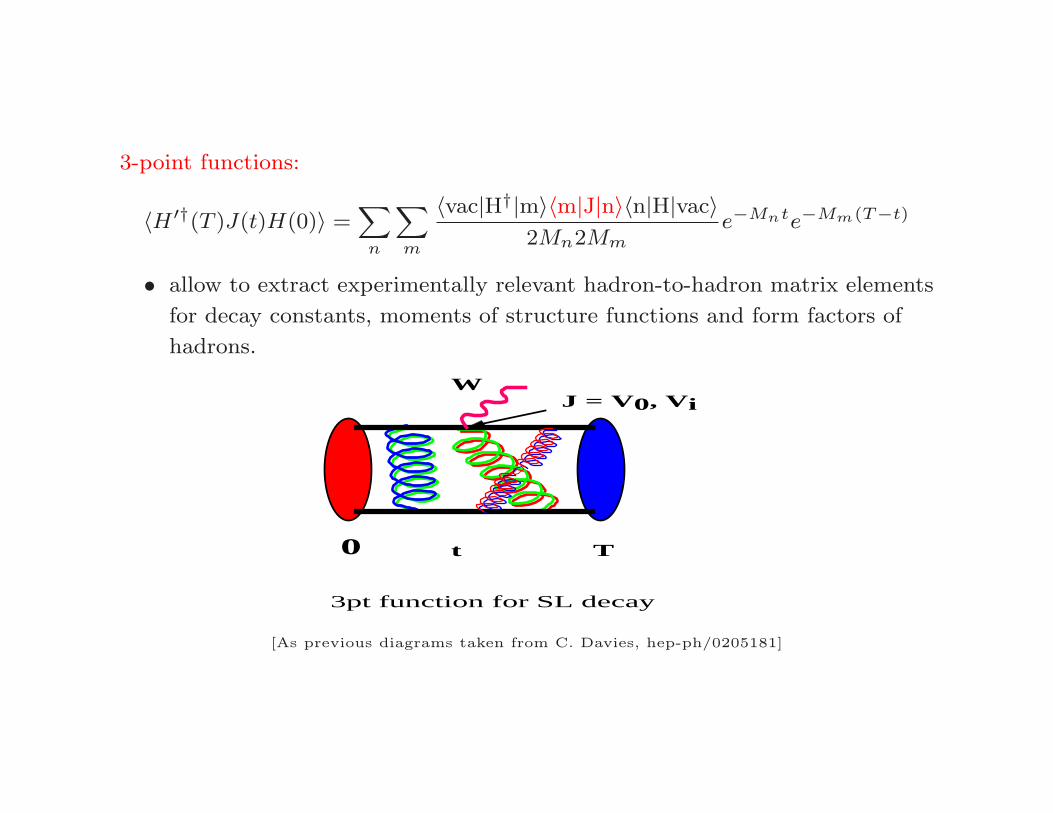
3-point functions:

〈H′†(T )J(t)H(0)〉 =∑

n

∑

m

〈vac|H†|m〉〈m|J|n〉〈n|H|vac〉2Mn2Mm

e−Mnte−Mm(T−t)

• allow to extract experimentally relevant hadron-to-hadron matrix elements

for decay constants, moments of structure functions and form factors of

hadrons.

WJ = V0, Vi

0 Tt

3pt function for SL decay

[As previous diagrams taken from C. Davies, hep-ph/0205181]

4th Lecture

6. Topology, Cooling and the Wilson (gradient) flow

6.1. Topology of gauge fields [Belavin, Polyakov, Schwarz, Tyupkin, ’75; ’t Hooft,

’76; Callan, Dashen, Gross, ’78 -’79]

Euclidean Yang-Mills action: S[A] = − 12g2

∫

d4x tr (GµνGµν)

Topological charge:

Qt[A] ≡∫

d4x ρt(x), ρt(x) = − 116π2 tr (GµνGµν(x)), Gµν ≡ 1

2ǫµνρσGρσ .

Qt[A] ≡q∑

i=1

wi ∈ Z ,

wi “windings” of continuous mappings S(3) → SU(2) (homotopy classes),

invariant w.r. to continuous deformations (but not on the lattice !!)

Example for topologically non-trivial field - “instanton”:

[Belavin, Polyakov, Schwarz, Tyupkin, ’75]

−∫

d4x tr [(Gµν ± Gµν)2] ≥ 0 =⇒ S[A] ≥ 8π2

g2|Qt[A]|

iff S[A] =8π2

g2|Qt[A]|, then Gµν = ±Gµν (anti) selfduality .

|Qt| = 1: BPST one-(anti)instanton solution (singular gauge) for SU(2):

A(±)a,µ (x− z, ρ, R) = Raαη

(±)αµν

2 ρ2 (x− z)ν

(x− z)2 ((x− z)2 + ρ2),

For SU(Nc) embedding of SU(2) solutions required.

Dilute instanton gas (DIG) −→ instanton liquid (IL):

path integral “approximated” by superpositions of (anti-) instantons and

represented as partition function in the modular space of instanton parameters.

[Callan, Dashen, Gross, ’78 -’79; Ilgenfritz, M.-P., ’81; Shuryak, ’81 - ’82; Diakonov, Petrov, ’84]

=⇒ may explain chiral symmetry breaking, but fails to explain confinement.

Case T > 0: x4-periodic instantons - “calorons”

Semiclassical treatment of the partition function [Gross, Pisarski, Yaffe, ’81]

with “caloron” solution ≡ x4-periodic instanton chain ( 1/T = b)

[Harrington, Shepard, ’77]

AaHSµ (x) = η

(±)aµν ∂ν log(Φ(x))

Φ(x)−1 =∑

k∈Z

ρ2

(~x− ~z)2 + (x4 − z4 − kb)2=

πρ2

b|~x− ~z|

sinh(

2πb |~x− ~z|

)

cosh(

2πb |~x− ~z|

)

− cos(

2πb (x4 − z4)

)

- Qt = − 116π2

∫ b0 dx4

∫

d3x ρt(x) = ±1 .

- (as for instantons) it exhibits trivial holonomy, i.e. Polyakov loop behaves as:

1

2trP exp

(

i

∫ b

0A4(~x, t) dt

)

|~x|→∞=⇒ ± 1

Kraan - van Baal solutions= (anti-) selfdual caloron solutions with non-trivial holonomy

[K. Lee, Lu, ’98, Kraan, van Baal, ’98 - ’99, Garcia-Perez et al. ’99]

P (~x) = P exp

(

i

∫ b=1/T

0A4(~x, t) dt

)

|~x|→∞=⇒ P∞ /∈ Z(Nc)

Action density of a single (but dissolved) SU(3) caloron with Qt = 1 (van Baal, ’99)

=⇒ not a simple SU(2) embedding into SU(3) !!

Dissociation into caloron constituents (BPS monopoles or “dyons”) gives hope

for modelling confinement for T < Tc as well as the deconfinement transition.

[Gerhold, Ilgenfritz, M.-P., ’07; Diakonov, Petrov, et al., ’07 - ’12; Bruckmann, Dinter, Ilgenfritz,

Maier, M.-P., Wagner, ’12; Shuryak, Sulejmanpasic, ’12-’13; Faccioli, Shuryak, ’13]

Systematic development of the semiclassical approach + perturbation theory

“resurgent trans-series expansions” ...

[Dunne, Unsal and collaborators, ’12-’14]

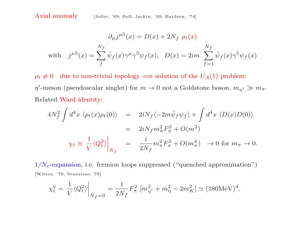
Axial anomaly [Adler, ’69; Bell, Jackiw, ’69; Bardeen, ’74]

∂µjµ5(x) = D(x) + 2Nf ρt(x)

with jµ5(x) =

Nf∑

f

ψf (x)γµγ5ψf (x), D(x) = 2im

Nf∑

f=1

ψf (x)γ5ψf (x)

ρt 6= 0 due to non-trivial topology =⇒ solution of the UA(1) problem:

η′-meson (pseudoscalar singlet) for m→ 0 not a Goldstone boson, mη′ ≫ mπ .

Related Ward identity:

4N2f

∫

d4x 〈ρt(x)ρt(0)〉 = 2iNf 〈−2mψfψf 〉+∫

d4x 〈D(x)D(0)〉

= 2iNfm2πF

2π +O(m2)

χt ≡1

V〈Q2

t 〉∣

∣

∣

∣

Nf

=i

2Nfm2πF

2π +O(m4

π) → 0 for mπ → 0.

1/Nc-expansion, i.e. fermion loops suppressed (“quenched approximation”)

[Witten, ’79, Veneziano ’79]

χqt =1

V〈Q2

t 〉∣

∣

∣

∣

Nf=0

=1

2NfF 2π [m2

η′ +m2η − 2m2

K ] ≃ (180MeV)4.

Integrating axial anomaly we get Atiyah-Singer index theorem

Qt[A] = n+ − n− ∈ Z

n± number of zero modes fr(x) of Dirac operator iγµDµ[A]with chirality γ5fr = ±fr.

=⇒ For lattice computations employ a chiral operator iγµDµ.=⇒ Not free of lattice artifacts, use improved gauge action.

Topology becomes unique only for lattice fields smooth enough.

Sufficient (!) bound to plaquette values can be given. [Luscher, ’82].

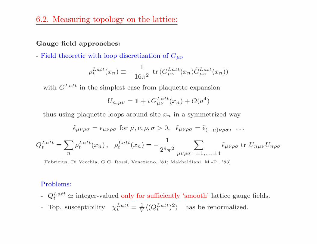
6.2. Measuring topology on the lattice:

Gauge field approaches:

- Field theoretic with loop discretization of Gµν

ρLattt (xn) ≡ − 1

16π2tr (GLattµν (xn)G

Lattµν (xn))

with GLatt in the simplest case from plaquette expansion

Un,µν = 1+ iGLattµν (xn) +O(a4)

thus using plaquette loops around site xn in a symmetrized way

ǫµνρσ = ǫµνρσ for µ, ν, ρ, σ > 0, ǫµνρσ = ǫ(−µ)νρσ , . . .

QLattt =∑

n

ρLattt (xn) , ρLattt (xn) = − 1

29π2

∑

µνρσ=±1,...,±4

ǫµνρσ tr UnµνUnρσ

[Fabricius, Di Vecchia, G.C. Rossi, Veneziano, ’81; Makhaldiani, M.-P., ’83]

Problems:

- QLattt ≃ integer-valued only for sufficiently ‘smooth’ lattice gauge fields.

- Top. susceptibility χLattt = 1V〈(QLattt )2〉 has be renormalized.

- Geometric definitions providing always integer Qt have been invented

[Luscher, ’82; Woit, ’83; Phillips, Stone, ’86],

(used with and without smoothing).

Fermionic approaches:

- Index of Ginsparg-Wilson fermion operators: Qt = n+ − n−

[Hasenfratz, Laliena, Niedermayer, ’98; Neuberger, ’01;... ]

- From corresponding spectral representation of ρt

ρt(x) = tr γ5(1

2Dx,x − 1) =

N∑

n=1

(λn

2− 1)ψ†

n(x)γ5ψn(x)

- Fermionic representation: [Smit, Vink, ’87]

NfQt = κ Trm γ5

D +m, κ renorm. factor

- Topological susceptibility from higher moments and spectral projectors

[Luscher, ’04; Giusti, Luscher, ’08; Luscher, Palombi, ’10; Cichy, Garcia Ramos, Jansen, ’13-’14

- .....

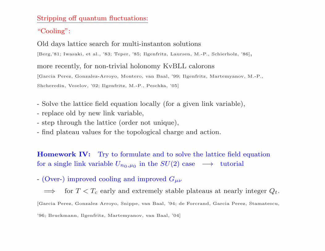
Stripping off quantum fluctuations:

“Cooling”:

Old days lattice search for multi-instanton solutions

[Berg,’81; Iwasaki, et al., ’83; Teper, ’85; Ilgenfritz, Laursen, M.-P., Schierholz, ’86],

more recently, for non-trivial holonomy KvBLL calorons

[Garcia Perez, Gonzalez-Arroyo, Montero, van Baal, ’99; Ilgenfritz, Martemyanov, M.-P.,

Shcheredin, Veselov, ’02; Ilgenfritz, M.-P., Peschka, ’05]

- Solve the lattice field equation locally (for a given link variable),

- replace old by new link variable,

- step through the lattice (order not unique),

- find plateau values for the topological charge and action.

Homework IV: Try to formulate and to solve the lattice field equation

for a single link variable Un0,µ0 in the SU(2) case −→ tutorial

- (Over-) improved cooling and improved Gµν

=⇒ for T < Tc early and extremely stable plateaus at nearly integer Qt.

[Garcia Perez, Gonzalez Arroyo, Snippe, van Baal, ’94; de Forcrand, Garcia Perez, Stamatescu,

’96; Bruckmann, Ilgenfritz, Martemyanov, van Baal, ’04]

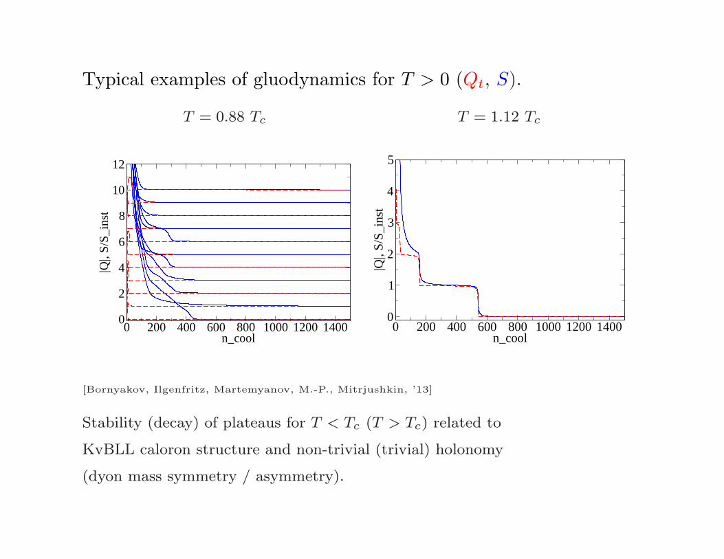
Typical examples of gluodynamics for T > 0 (Qt, S).

T = 0.88 Tc T = 1.12 Tc

0 200 400 600 800 1000 1200 1400n_cool

0

2

4

6

8

10

12

|Q|,

S/S_

inst

0 200 400 600 800 1000 1200 1400n_cool

0

1

2

3

4

5

|Q|,

S/S_

inst

[Bornyakov, Ilgenfritz, Martemyanov, M.-P., Mitrjushkin, ’13]

Stability (decay) of plateaus for T < Tc (T > Tc) related to

KvBLL caloron structure and non-trivial (trivial) holonomy

(dyon mass symmetry / asymmetry).

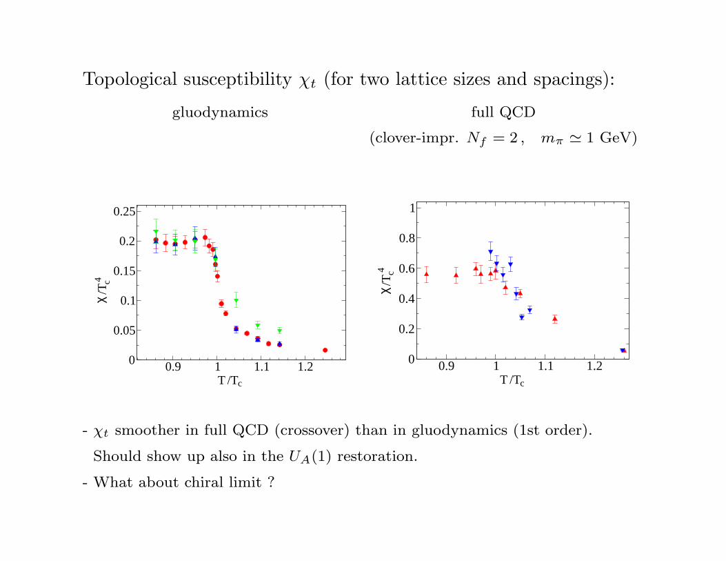
Topological susceptibility χt (for two lattice sizes and spacings):

gluodynamics full QCD

(clover-impr. Nf = 2 , mπ ≃ 1 GeV)

0.9 1 1.1 1.20

0.05

0.1

0.15

0.2

0.25

χ/T

c4

/TT c

0.9 1 1.1 1.20

0.2

0.4

0.6

0.8

1

χ/T

/TT c

c4

- χt smoother in full QCD (crossover) than in gluodynamics (1st order).

Should show up also in the UA(1) restoration.

- What about chiral limit ?

Wilson or gradient flow:

Proposed and thoroughly investigated by M. Luscher

(perturbatively with P. Weisz) since 2009 (cf. talks at LATTICE 2010 and 2013).

Flow time evolution uniquely defined for arbitrary lattice field Uµ(x) by

Vµ(x, τ) = −g20[

∂x,µS(V (τ))]

Vµ(x, τ), Vµ(x, 0) = Uµ(x) .

- Diffusion process continuously minimizing action, scale λs ≃√8t, t = a2τ .

- Allows efficient scale-setting (t0, t1)

by demanding e.g. t2〈− 12tr GµνGµν〉|t=t0,t1 = 0.3, 2

3.

- Emergence of topological sectors at sufficient large length scale becomes clear.

- Renormalization becomes simple (in particular in the fermionic sector).

=⇒ Easy to handle, theoretically sound prescription !!

How does it work? [Bonati, D’Elia, arXiv:1401.2441 [hep-lat]]

Wilson plaquette action:

S =2Nc

g20

∑

x,µ<ν

(

1− 1

2Nctr (Uµν(x) + U†

µν(x))

)

,

“Staples” = (in general non unitary) matrices Wµ(x), defined by

Wµ(x) =∑

ν 6=µ

[

Uν(x)Uµ(x+ ν)U†ν (x+ µ) + U†

ν (x− ν)Uµ(x− ν)Uµ(x− ν + µ)

]

Part of action involving a given link variable Uµ(x):

−(2/g20) Re tr [Uµ(x)W†µ(x)] ≡ −(2/g20) Re tr [Ωµ(x)] = −(1/g20) tr [Ωµ(x)+Ω†

µ(x)]

Link derivatives (with Hermitean generators Ta):

∂(a)x,µ f(Uµ(x)) =

d

dsf(eisT

aUµ(x))

∣

∣

∣

∣

s=0

∂(a)x,µ S(U) =

2

g20Im tr

[

TaΩµ]

g20 ∂x,µS(U) ≡ 2i∑

a

Ta Im tr[

TaΩµ]

=1

2

(

Ωµ − Ω†µ

)

− 1

2Nctr(

Ωµ − Ω†µ

)

.

Comparison gradient flow with cooling: [C. Bonati, M. D’Elia, 1401.2441]

Pure gluodynamics:

- For given number of cooling sweeps nc find gradient flow time τ

yielding same Wilson plaquette action value.

- Perturbation theory: τ = nc/3

τ/nc scaling χ14t vs. λs

0 5 10 15 20 25 30nc

0

2

4

6

8

10

τ(n c

)

β=5.95β=6.07β=6.2

0 0.2 0.4 0.6 0.8 1 1.2 1.4 1.6

λS [fm]

192

194

196

198

200

χ1/4 [

MeV

]

gradient flow β=5.95gradient flow β=6.07gradient flow β=6.2cooling β=5.95cooling β=6.07cooling β=6.2

- Lattice spacing dependence at fixed λs clearly visible.

- Moreover: cooling and gradient flow show same spatial topological structure.

Holds also for ρt(x) filtered with adjusted # ferm. (overlap) modes

[Solbrig et al., ’07; Ilgenfritz et al., ’08].

7. Conclusions, outlook

• Have discussed the basics of lattice gauge theories.

• Main aim was the introduction of lattice QCD.

• As main features were discussed:

– the path integral method, in particular for fermion matter fields;

– Wilson’s representation of gauge fields on the lattice, such that gauge

invariance is maintained;

– the continuum limit on the basis of the renormalization group and

‘asymptotic freedom’.

• Basic Monte Carlo methods for the pure gauge case were introduced.

• The basic approach to compute hadron correlation functions was

presented.

• QCD at non-zero temperature was introduced.

• Methods to reveal the topological structure of QCD were presented.

Introduction to Lattice Gauge Theories...

Documents

Transcript of Introduction to Lattice Gauge Theories...