Introduction to Kohn-Sham Density Functional Theory ... · Introduction to Kohn-Sham Density...

Introduction to Kohn-Sham Density FunctionalTheory: Analysis and Algorithms

Weinan E 1 and Jianfeng Lu 2

1Princeton University

2Courant Institute of Mathematical SciencesNew York University

Collaborators: Roberto Car, Carlos Garcıa-Cervera, Weiguo Gao,Lin Lin, Juan Meza, Chao Yang, Xu Yang, Lexing Ying.

Fundamentals

Macroscopic limit of density functional theoryDerivation of nonlinear elasticity and macroscopic electrostaticequation from Kohn-Sham DFTDerivation of macroscopic Maxwell equation from TDDFT

AlgorithmsIntroductionDiscretization of the Kohn-Sham HamiltonianRepresentation of the Fermi OperatorDensity evaluation

Quantum many-body problem

The (non-relativistic) ground state electronic structure of a systemis determined by the lowest eigenvalue and eigenfunction of themany-body time independent Schrodinger operator (omitting spin):

HΨ =(∑

i

−12 ∆xi +

∑i<j

1

|xi − xj |−∑i ,α

Zα|xi − Xα|

)Ψ = E Ψ,

within the Born-Oppenheimer approximation.

E (Xα) = inf‖Ψ‖=1

〈Ψ|H|Ψ〉.

Here the many-body wave function Ψ(x1, x2, . . . , xN) is anantisymmetric function of N variables, according to Pauli’sexclusion principle.

Reduction of the quantum many-body problem

Due to curse of dimensionality, the many-body problem ispractically impossible to solve, except for tiny systems.Reductions based on various approximations:

I Discrete lattice approximation: Tight-binding models.

I Low-rank approximation: Hartree-Fock; ConfigurationalInteraction; Multi-configurational self-consistent field(MCSCF);

I Mean-field approximation: Density functional theory (DFT);

I Coupled clusters;

I Others ...

Most are not systematic approximations to the many-bodyproblem.

Tight-binding model

Consider one-body effective Hamiltonian, and assume one-bodywave functions take the form

ψ(x) =∑α,i

ci ,αϕi (x − Xα),

where ϕi are atomic orbitals. Similar to a generalized finiteelement discretization.

Hence, the Hamiltonian becomes a matrix acting on ci ,α.

Nonlinear tight-binding model is also used sometimes. Theeffective Hamiltonian depends on the density (like a discreteversion of density functional theory)

Hartree-Fock theory

Assumes the many-body wave function is a single Slaterdeterminant

Ψ =1√N!

det

∣∣∣∣∣∣∣∣∣ψ1(x1) ψ2(x1) · · · ψN(x1)ψ1(x2) ψ2(x2) · · · ψN(x2)

......

. . ....

ψ1(xN) ψ2(xN) · · · ψN(xN)

∣∣∣∣∣∣∣∣∣with ψi a set of orthonormal functions.

For example, in this approximation, the kinetic energy reduces to∫R3N

Ψ∗(−∑

i

12 ∆xi )Ψ =

∑i

1

2

∫R3

|∇ψi (x)|2.

Hartree-Fock theory (cont’d)

Hartree-Fock equation(−1

2∆ + Vext +

∫R3

ρ(y)

|x − y |dy −K

)ψi = λiψi .

K is the exchange operator:

Kψi =

∫ψ∗j (y)ψi (y)

|x − y |dyψj(x).

As the energy is minimized over a smaller space,

E ≤ EHF = E + Ec .

The error made Ec is called correlation energy, as a result ofignoring many-body interactions (besides Coulomb and exchange).

Density functional theory

Brief history:

I Thomas-Fermi: Concepts of using solely the density todescribe quantum mechanics (simple empirical models).

I Hohenberg-Kohn: Proves that for ground state in quantummechanics is indeed only a function of the electron density.

I Kohn-Sham: Mean field theory for non-interacting electrons inan effective potential.

I Levy-Lieb variational principle: Mathematical rigorousfoundation.

I Development of exchange-correlation functional (Becke,Burke, Ernzerhof, Parr, Perdew, Yang, ...)

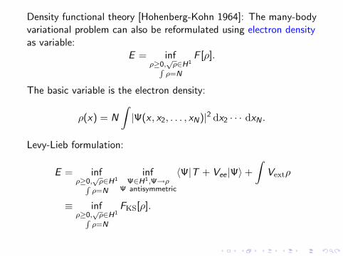
Density functional theory [Hohenberg-Kohn 1964]: The many-bodyvariational problem can also be reformulated using electron densityas variable:

E = infρ≥0,

√ρ∈H1R

ρ=N

F [ρ].

The basic variable is the electron density:

ρ(x) = N

∫|Ψ(x , x2, . . . , xN)|2 dx2 · · · dxN .

Levy-Lieb formulation:

E = infρ≥0,

√ρ∈H1R

ρ=N

infΨ∈H1,Ψ→ρ

Ψ antisymmetric

〈Ψ|T + Vee |Ψ〉+

∫Vextρ

≡ infρ≥0,

√ρ∈H1R

ρ=N

FKS[ρ].

Kohn-Sham density functional theory

The energy functional depends on N electron orbitals ψi:

FKS(ψi) =∑

i

1

2

∫|∇ψi |2

+1

2

∫∫(ρ−m)(x)(ρ−m)(y)

|x − y |+ Exc[ρ].

The orbitals are orthonormal, ρ is the electron density given byρ(x) =

∑i |ψi (x)|2. m is the background charge distribution.

Formally exact. All errors are encoded in the last term, theexchange-correlation energy, which contains chemistry, as itmodels the quantum correlation of electrons. However, the explicitform is unknown and needs approximation.

Input to the model

Background charge: m(y) =∑

yj∈Ω maj (y − yj)

I yj = positions of the nuclei (ions).I ma

j = ionic potential describing the atoms in the system.I All electron model: ma

j = delta functionI Valence electron model (view core electrons as part of the

nuclei): maj is (local) pseudopotential.

I Chemistry: yj ,maj describes a set of molecules.

I Materials: yj ,maj describes a deformed lattice with defects.

Local density approximation

In principle Exc[ρ] is a nonlocal functional depending on ρ. In thelocal density approximation, it is assumed that Exc[ρ] is a localfunctional:

Exc[ρ] =

∫εxc(ρ(x)) dx .

Taking LDA, the energy functional becomes

FKS(ψi) =∑

i

1

2

∫|∇ψi |2

+1

2

∫∫(ρ−m)(x)(ρ−m)(y)

|x − y |+

∫εxc(ρ(x)).

The function εxc is obtained from calculations of Jellium system.

εxc(ρ) = −ρ4/3 + ...

.

Developments about exchange-correlation functional

I Theoretically, it is a universal functional of the density field.

I In practice, it is obtained by physics intuition and argument,plus fitting from quantum Monte Carlo calculations.

I Examples of functional forms: Becke88, LYP, PBE, so on;

I Jacob’s ladder of exchange-correlation energy: meta-GGA(TPSS), hybrid functionals (B3LYP), etc.

Question: Mathematical derivations? Which asymptotic regime?(Burke, Friesecke, Solovej, ...)

Alternative formulations

Several alternative formulations for the Kohn-Sham densityfunctional theory:

I orbitals or wavefunctions

I density matrix or projection operator, or subspace formulation

I density (in terms of the Kohn-Sham map)

Subspace problem

The energy functional FKS(ψj) is invariant under rotations ofthe wave functions. More generally, define the non-orthogonalenergy functional as

FKS(ψi) =∑ij

1

2

∫∇ψ∗i S−1

ij ∇ψ∗j

+1

2

∫∫(ρ−m)(x)(ρ−m)(y)

|x − y |+

∫εxc(ρ(x)).

with Sij = 〈ψi , ψj〉 and ρ(x) =∑

ij S−1ij ψ∗i (x)ψj(x). The energy

functional is invariant under general non-degenerate lineartransformation.

The Kohn-Sham density functional theory is a minimization overoccupied subspace. The particular basis ψj is not relevant.

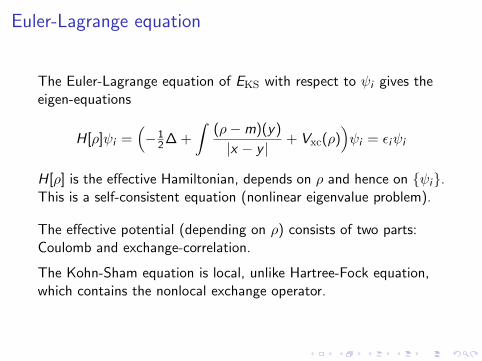
Euler-Lagrange equation

The Euler-Lagrange equation of EKS with respect to ψi gives theeigen-equations

H[ρ]ψi =(−1

2 ∆ +

∫(ρ−m)(y)

|x − y |+ Vxc(ρ)

)ψi = εiψi

H[ρ] is the effective Hamiltonian, depends on ρ and hence on ψi.This is a self-consistent equation (nonlinear eigenvalue problem).

The effective potential (depending on ρ) consists of two parts:Coulomb and exchange-correlation.

The Kohn-Sham equation is local, unlike Hartree-Fock equation,which contains the nonlocal exchange operator.

Kohn-Sham map

Given an effective Hamiltonian H[ρ], the density corresponding tothe occupied states can be written as

ρ(x) = φ0FD(H[ρ]− µ)(x , x)

where φ0FD(x) = χx≤0 is the Heaviside function, Fermi-Dirac

distribution at zero temperature. µ is the chemical potential,suitably chosen so that

∫ρ = N.

The map from ρ to ρ is called Kohn-Sham map F .

This is extended to the finite temperature case by takingFermi-Dirac distribution function instead of the Heaviside functionin the above (corresponds to Mermin functional).

Orbital free density functional theory

The orbital-free density functional theory is a further simplificationof the Kohn-Sham DFT so that the functional only involves thedensity.

In particular, the kinetic energy functional is replaced by afunctional depends on ρ only, approximates

T [ρ] = infψj7→ρ

∑j

∫R3

|∇ψj |2 dx .

I Thomas-Fermi approximation:∫

R3 ρ5/3 dx .

I Thomas-Fermi-von Weiszacker approximation:∫

R3 ρ5/3 dx +∫

R3 |∇√ρ|2 dx based on gradient expansion.

I Wang-Teter and Wang-Govind-Carter functionals based onlinear response.

On the mathematical level, the nature of orbital-based andorbital-free DFTs are quite different.

The orbital-free DFT is more of a conventional variational problemin applied mathematics, like Landau-Lifschitz, Ginzburg-Landau,liquid crystals, nonlinear elasticity and so on.

We will focus mainly on orbital-based Kohn-Sham densityfunctional theory from now on.

Issues of Kohn-Sham density functional theory

On the analysis side:

I Existence is not trivial due to possible loss of compactness;

I Uniqueness is not always expected as the functionals arenon-convex;

I The property and structure of the solutions are not easy toinvestigate.

On the numerics side:

I Conventional cubic scaling algorithms is too expensive.Calls for fast algorithms and efficient parallelization to addresslarge systems.

I Choices of discretization to achieve the balance betweenaccuracy and efficiency;

I Issue of numerical analysis: accuracy, convergence, so on.

Existence and uniqueness results

Existence of minimizer of the energy functional:

I Existence of DFT with LDA approximation [Le Bris 1993]

I Existence of DFT with GGA approximation (one orbital case)[Anantharaman-Cances 2009]

Existence and uniqueness of finite temperature Kohn-Shamequation: [Prodan-Nordlander 2003]

Fundamentals



Motivation

Physical systems (solids, materials) can be modeled at differentscales:

I Quantum mechanics: Many-body Schrodinger equation,electronic structure models, lattice models, ...

I Atomistic models: Molecular statics and dynamics withempirical potentials;

I Continuum theories: Elasticity, dielectricity, micromagnetism,phase field models, ...

Multiscale modeling and analysis: Understanding the connectionsand coupling between models on different scales.

Continuum theories

We will focus on in this talk two representatives of continuummodels:

I Nonlinear elasticity:

infu

∫W (∇u(x))− f (x)u(x) dx .

I Macroscopic Maxwell equation:

∇ · D = ρf ,

∇ · B = 0,

∇× E = −∂tB,

∇× H = Jf + ∂tD;

The continuum theories are obtained by physical principle(minimum action principle, conservation laws, ...) plus empiricalconstitutive relations.

Macroscopic limit

Want to understand the following questions for the connectionsbetween micro and macro models:

I How can we obtain the constitutive relations of themacroscopic models from the microscopic ones?

I When are the macroscopic models valid characterizations ofthe system?

I How does the failure of the macroscopic models happen?What is the onset of breaking down?

For example, elasticity theory → plasticity, fracture.

These questions can be addressed by studying macroscopic limit ofmicroscopic models.

Fundamentals



Related works

For perfect crystal, the thermodynamic limit was studied

I for KSDFT model without exchange-correlation[Catto-Le Bris-Lions 2001].

For perfect crystal with local defects, the macroscopic limit wasstudied

I for KSDFT model without exchange-correlation[Cances-Deleurence-Lewin 2009, Cances-Lewin 2010].

For elastically deformed crystal, the macroscopic limit was studied

I for KSDFT model [E-Lu preprint].

Derivation of nonlinear elasticity and macroscopicelectrostatic equation from DFT

For Kohn-Sham DFT, under sharp stability conditions

I The equilibrium system is insulating;

I The equilibrium system is stable with respect to plasmons;

I The effective dielectric constant for the equilibrium system ispositive definite,

the electronic structure for the elastically deformed system ischaracterized by the Cauchy-Born rule (the electron density andlocal energy density is determined by the local deformationgradient).

The dielectric response of the system couples with the elasticdeformation (sort of piezoelectric effects), and is characterized byan effective Poisson equation.

Cauchy-Born rule for electronic structureCauchy-Born rule is a recipe links together micro- and macro-scalemodels.

Main idea: On the microscopic scale, the smooth macroscopicelastic displacement is effectively linear. Hence, at each point x ,the energy density and also other physical quantities should begiven by those of a system with homogeneous deformation withdeformation gradient ∇u(x) (Independent of u(x) due tosymmetry invariance).

Smoothly deformed crystal

Assumption: Atoms follow the prescribed smooth displacementfield u.

At equilibrium, the atoms form a crystal εL, with underlyingBravais lattice εL and unit cell εΓ. Take a smooth Γ-periodicdisplacement field u(x), so that under deformation the atoms arelocated at Y ε

i = X εi + u(X ε

i ), where X εi ∈ εL.

Remarks about periodicity of u:

I The period gives the characteristic length of u: O(1);

I With the PBC assumption, only the bulk behavior is present.The interesting surface phenomenon (e.g., surface plasmon) isruled out.

Continuum limit

The small parameter ε is understood as the ratio between thelattice constant (atomic length scale) and the characteristic lengthscale of the elastic deformation.

The continuum limit ε→ 0 will be considered. Physically, theatomic spacing is tiny compared to the macroscopic deformation.

Questions:

I Derivation of nonlinear elasticity from KSDFT;

I Characterization of the electronic structure for deformedcrystals;

I Identification of the onset of failure of nonlinear elasticitymodel (sharp stability conditions).

Electronic structure for perfect crystalAt equilibrium, we assume there exists a Γ-periodic electron densityρe , such that

ρe(x) = F (ρe)(x) =1

2πi

∫C

1

λ− He [ρe ]dλ(x , x).

The effective potential Ve is also Γ-periodic and one can apply theBloch-Floquet theory

He =

∫Γ∗

Hξ dξ, Hξ =∑n

En(ξ)|ψn,ξ〉〈ψn,ξ|.

We assume that the system under consideration is an insulator:

dist(σZ , σ(He)\σZ ) = Eg > 0

where σZ =⋃

n≤Z En(Γ∗). Therefore, the Kohn-Sham map is welldefined (through Bloch-Floquet theory) for a compact contour Cencloses the occupied spectrum.

Change of coordinates

Electrons live in the Eulerian coordinates, while atoms live in theLagrangian coordinates. For our problem (elasticity for solids), it ismore convenient to put the electronic structure problem in theLagrangian coordinates.

The deformation is given by τ(x) = x + u(x), and hence thepullback and pushforward operators between Eulerian andLagrangian coordinates are

(τ∗f )(x) = f (τ(x)), (τ∗g)(y) = g(τ−1(y)).

Effective Hamiltonian operatorHamiltonian (in the Lagrangian coordinates):

Hετ = −ε2J1/2∆τJ−1/2 + V ε

τ (x)

with ∆τ = τ∗∆τ∗ and J(x) = det(∇τ(x)).

Potential (Coulomb + exchange-correlation):

V ετ [ρ](x) = φετ [ρ](x) + η(J(x)−1ε3ρ(x));

−∆τφετ [ρ] = 4πεJ−1(ρ−mετ );∫

Γφετ [ρ] dx = 0.

The deformation u enters through the background chargedistribution:

mετ (x) = J(x)

∑X εα∈εL

1

ε3ma((τ(x)− τ(X ε

α))/ε)

Kohn-Sham equation

Look for fixed point of the Kohn-Sham map for the deformedsystem:

ρ(x) = F ετ (ρ)(x) =

1

2πi

∫C

1

λ− Hετ [ρ]

dλ(x , x).

Here C is a fixed contour in the resolvent set of the Hamiltonianenclosing the occupied spectrum.

The right hand side is the diagonal of kernel of a operator (not intrace class), which is not a priori well defined. Nevertheless, it canbe proved to be well defined for the cases we will consider byelliptic regularity results.

Cauchy-Born rule for electron density

For the system deformed homogeneously with deformation gradientA = ∇u(x0), we still have a periodic problem.

By implicit function theorem + stability condition, when |A| issufficiently small, there exists a solution to the Kohn-Shamequation, denoted as ρCB(x ; A). Also, ρCB(·; A) is Γ-periodic (asdefined in Lagrangian coordinates).

According the Cauchy-Born philosophy, one expects

ρε(x) ∼ ε−3ρCB(x/ε;∇u(x)).

In other words, electron density is given locally by that of thehomogeneous deformed system.

Locality of quantum system

Recall that the quantum mechanical model is a rather nonlocalfrom the first sight.

I Coulomb interaction is nonlocal;

I The Pauli exclusion principle (orthogonal constraint) isnonlocal;

I The Schrodinger eigenvalue problem is nonlocal.

Nevertheless, the Cauchy-Born rule states that the electronicstructure at a point only depends on the local surroundingenvironment. This is related with the property of“near-sightedness” in the physics literature: for insulators, thephysics is essentially local [Kohn 1996, Prodan-Kohn 2005].

Stability conditions

The Cauchy-Born rule is valid under sharp stability conditions. Inother words, the electron density is well approximated by theCauchy-Born guess, provided that the equilibrium system is stable:

I Stability of band gap: The equilibrium system is a bandinsulator.

I Stability wrt charge density wave: The linearized Kohn-Shamoperator is invertible in suitable spaces.

I Stability of dielectric response: The permittivity tensor ispositive definite (The effective Poisson equation is elliptic).

Stability conditions

We will assume that the electronic structure is stable, in the senseof the following two assumptions.

Assumption (Stability of charge density wave)

For every n ∈ N, I − Le as an operator on H−1n ∩ H2

n is invertible,and the norm of its inverse is bounded independent of n:

‖(I − Le)−1‖L (H−1n ∩H2

n ) . 1.

Assumption (Stability of dielectric response)

The effective permittivity tensor E is positive definite.

Stability of dielectric response

Recall E = 12 (Ae + A∗e) + 1

4π I is the macroscopic permittivitytensor for the undeformed crystal.

The matrix Ae = (Ae,αβ) for α, β = 1, 2, 3 is given by

Ae,αβ =− 2<∑n≤Z

∑m>Z

∫Γ∗

dξEn(ξ)− Em(ξ)

×⟨um,ξ, ∂ξβun,ξ

⟩⟨um,ξ, ∂ξαun,ξ

⟩− 〈ge,α, δρe Ve(I − Le)−1ge,β〉,

and

ge,α(z) = 2<∑n≤Z

∑m>Z

∫Γ∗

dξEn(ξ)− Em(ξ)

× u∗n,ξ(z)um,ξ(z)⟨um,ξ, i∂ξαun,ξ

⟩;

Linearized Kohn-Sham map

Consider the linearization of the Kohn-Sham map Fe at theequilibrium density ρe . Formally, Lew → Le(w), where

Le(w) =1

2πi

∫C

1

λ−He(ρe)δρe Ve(w)

1

λ−He(ρe)dλ(x , x).

Here δρe Ve is the linearized operator of Ve(ρ) at ρe , given by (fornΓ-periodic function w)

δρe Ve(w)(x) = δφe(w)(x) + η′(ρe)w(x);

−∆δφe(w)(x) = 4πw ,

with periodic boundary condition on nΓ and∫nΓ δφe = 0 to fix the

arbitrary constant.

Spaces of periodic functionsFor a given n, define the periodic Sobolev space

W m,pn (R3) = f ∈ S ′(R3) | τR f = f , ∀R ∈ nL; f ∈W m,p(nΓ)

with its natural norm ‖f ‖W m,pn (R3) = ‖f ‖W m,p(nΓ). We will also

write Hmn for W m,2

n . Here, (τR f )(x) = f (x − R).

Moreover, define the periodic Coulomb space (homogeneousSobolev space with index −1) H−1

n (R3) as

H−1n (R3) = f ∈ S ′(R3) | τR f = f , ∀R ∈ nL;∑

k∈L∗/n

1

|k|2|f (k)|2 <∞.

Here, f (k) denotes the Fourier coefficients of the nΓ-periodicfunction f . Also the higher order spaces Hm+1

n , defined by thenorm

‖f ‖Hm+1n (R3) = ‖∇f ‖Hm

n (R3)3 .

Analysis of the linearized Kohn-Sham map

Theorem (Uniform boundedness of Le)

The operator Le is bounded on spaces H−1n ∩ H2

n uniformly in n.

Write Lew = χeδρe Vew with the polarizability operator

(χeV )(x) =1

2πi

∫C

1

λ−HV

1

λ−Hdλ(x , x).

The proof consists of showing

I δρe Ve : H−1n ∩ H2

n → H2n + H4

n is uniformly bounded;

I χe : H2n + H4

n → H−1n ∩ H2

n is uniformly bounded.

Polarizability operator

One may represent χe in more explicit terms:

χeV = 2<∑n≤Z

∑m>Z

∫(Γ∗)2

dξ dζ 〈ψn,ξ,Vψm,ζ〉En(ξ)− Em(ζ)

ψn,ξψ∗m,ζ .

For example, for Jellium model (H = −∆), we have

χeV (k) = m(k)V (k),

where

m(k) =1

8βπ2k

∫ ∞0

d``

ln

(1 + e−β((`− k/2)2 − µ)

1 + e−β((`+ k/2)2 − µ)

).

We remark that the behavior the linearized Kohn-Sham map israther different for metal and insulator. In particular, theboundedness results only hold for insulators (due to a finite bandgap).

Ingredients of the estimate for χe :I L1

n → L1n: Show the operator is in trace class, using

‖f (x)g(−i∇ξ)‖Sp(L2n) . ‖f ‖Lp

n‖g‖lp(L∗/n),

I L∞n → L∞n : Based on Agmon type’s argument of regularity ofkernel of elliptic operators.

I H2n → H2

n : Estimates of commutators.I H1

n → H−1n : Based on the generalized trace class technique

[Hainzl-Lewin-Sere 2005, Cances-Deleurence-Lewin 2008].I H3

n → H2n : Uses the “trick of projection”

QV =1

2πi

∫C

1

λ−HV

1

λ−Hdλ

=1

2πi

∫CP 1

λ−HV

1

λ−HP⊥ dλ

+1

2πi

∫CP⊥ 1

λ−HV

1

λ−HP dλ,

where P is the projection operator on the occupied space.

What happens when the stability condition is violated?

Instability of charge density wave (plasmon instabilities):

I Wigner crystal: Crystal formation of Fermi gas at low density

I Change of lattice structure: The electrons and nuclei mayhave different (and possibly incommensurate) crystalstructures

I Defects formation: Possibility to have electronic defects (inanalogy to crystal defects).

More on stability

There are three scales of instability in the system (electronic,atomic and continuum). Due to our assumption that the atomsfollow the smooth displacement, we are only looking at thestability of electronic structure.

Without the assumption, the situation becomes more complicated.Then the system could present instability in electronic structureand also instability in atom positions (phonon analysis).

It is of interest to identify the boundary of these instabilities.Questions like whether the atomistic stability still holds while theelectronic structure become unstable.

Main results

Theorem (E-Lu, preprint)

Under stability assumptions, there exist constants a, ε0 and M,such that if ε ≤ ε0 and if MA = supj‖∇ju‖L∞ ≤ a, then thereexists ρε ∈ L∞ε with the property:

I ρε is a solution to the Kohn-Sham equation:

ρε(x) = Fετ (ρε)(x).

I ‖ρε − ε−3ρCB(x/ε;∇u(x))‖L∞ε ≤ Mε1/2, i.e.,

‖ρε − ρCB(x ;∇u(εx))‖L∞ ≤ Mε1/2, where ρε(x) = ε3ρ(εx),and ρε satisfies the normalization constraint:∫

Γρε(x) dx = Zε−3.

Theorem (E-Lu, preprint)

I Moreover, The macroscopic potential satisfies a second-orderelliptic equation of the form:

Aαβ∂xα∂xβU0(x) + 14πL2U0(x) + Bα∂xαU0(x)

+ D− 〈m2(x , ·)〉 = 0

This is a piezo-electric effect: Mechanical deformationintroduces an electric potential.

Sketch of the proof

General strategy:

I Build a higher order approximated solution to the Kohn-Shamequation ρ0 using asymptotic expansion:

ρ0 = ε−3ρCB(x/ε;∇u(x)) + ε−2ρ1(x , x/ε) + · · ·

I Start from the approximated solution ρ0, use Newton iterationto find the unique fixed point nearby. The stability conditionguarantees the convergence and uniformality with ε.

The overall strategy is standard, but technically both steps arenon-conventional and require careful analysis.

Some remarks

I The Cauchy-Born rule for the energy and also the expressionfor the stored energy density follow.

I To simplify the presentation, the result is not written in itsoptimal form. In particular, the norm can be sharpened intoH−1ε ∩ H2

ε and higher order approximation can be constructed.

I The effective permittivity at macroscopic level has beenstudied for undeformed crystal in reduced Hartree-Fock modelin [Cances-Lewin 2010], in the cases that the amplitude of theexternal potential is small (linear perturbation regime).

Characterization of the occupied space

We know that for the perfect crystal, the electronic structure canbe understood by Bloch-Floquet theory, which gives a clearpicture. In particular, the occupied space can be represented by theBloch wave functions ψn,ξ(x).

Hξψn,ξ = En,ξψn,ξ.

Another useful set of basis functions for the occupied space isWannier functions

Wn,R(x + R ′) =

∫Γ∗

e iξ·(R′−R)ψn,ξ(x) dξ,

The Wannier functions decays exponentially for band insulators[Kohn 1959, Nenciu 1983, Panati 2007].

Wannier functions for deformed crystals

How about deformed crystals that translational symmetry isbroken? The Bloch-Floquet theory no long applies. What is thegeneralization of Wannier functions?

Project Wannier functions for the equilibrium state onto theoccupied space of the deformed system.

Let W εe,k be the set of (rescaled) Wannier functions for the

equilibrium configuration. The projected Wannier functions

W ετ,k = Pε

τW εe,k

form a basis for the occupied space for Hετ provided that the

displacement is small. The functions W ετ,k are still exponentially

localized.

Cauchy-Born rule for the projected Wannier functions

Denote the center of the Wannier function for the equilibriumconfiguration W ε

e,k as centered at cεk = εck .Take the Wannier function associated with the homogeneouslydeformed system: W ε

A(cεk ),k with A(cεk) = ∇u(cεk).

Theorem (E-Lu, 2010)

Under the same assumption as the previous theorem, we have

‖(I + ε2∆)(W ετ,k −W ε

A(cεk ),k)‖L2 ≤ Cε.

In other words, the Cauchy-Born construction gives a goodapproximation to the Wannier functions of the deformed system.The Wannier functions are stable under deformation.

Example of Cauchy-Born rule for Wannier functions

Figure: Example of Cauchy-Born rule construction of Wannier functions:Parameter ε = 1/32

Fundamentals



Time dependent density functional theory

Time dependent (current) density functional theory:

i~∂ψj

∂t=

1

2me

(−i~∇− e

c(A + Aext)

)2ψj + e(V + Vext)ψj ,

−∆φ =e

ε0(ρ−m),

1

c

∂

∂t

(1

c

∂

∂tA +∇φ

)−∆A =

e

cε0J,

∇ · A = 0,

V (t, x) = φ(t, x) + η(ρ(t, x)),

Model assumptions:

I ALDA approximation for exchange-correlation scalar potential;

I No exchange-correlation vector potential;

I Spin degeneracy is ignored.

Time dependent density functional theory (cont’d)

The electron density and current are given by

ρ(t, x) =N∑

j=1

|ψj(t, x)|2,

J(t, x) =~

me

N∑j=1

=(ψ∗j (t, x)∇ψj(t, x))− e

mecρ(t, x)A(t, x).

The system describes the quantum dynamics of electrons under theeffect of external potentials Aext and Vext.

The system consists of nonlinear Schrodinger equations (manyelectrons) coupled with microscopic (vacuum) Maxwell equations.

Nondimensionalization and macroscopic scalingWe consider the physical situation that the external fields Vext andAext are slowly varying in space. Denotes ε as the small parametercharacterizing the ratio between the lattice parameter and theexternal fields.

i∂ψj

∂t=

1

2(−iε∇− ε(A + Aext))2 ψj + (V + Vext)ψj ,

−∆φ = ε(ρ−m),

∂2

∂t2A−∆A +

∂

∂t∇φ = ε2J,

∇ · A = 0,

V (t, x) = φ(t, x) + η(ε3ρ(t, x)).

ρ(t, x) =∑|ψj(t, x)|2,

J(t, x) = ε∑=(ψ∗j (t, x)∇ψj(t, x)

)− ερ(t, x)A(t, x).

Macroscopic limit

Assume that without external fields, the ground state of thesystem forms a perfect lattice and is an insulator (finite gap in thespectrum).

Questions:

I Derivation of macroscopic Maxwell equation, in particular, theconstitutive relations;

I Identification of sharp stability conditions (future work);

I Dynamic coupling of elastic deformation and electromagneticfields (future work).

[E, Lu and Yang, in press]

Macroscopic Maxwell equation

By asymptotic analysis, the following macroscopic Maxwellequation is obtained in the macroscopic limit:

∇ ·(E(ω)E (ω, x)

)= ρext(ω, x),

∇ · B(ω, x) = 0,

∇× E (ω, x) = iωB(ω, x),

∇× B(ω, x) = −iωE(ω)E (ω, x) + Jext(ω, x),

with ρext, Jext given by Vext and Aext.

Here the effective dynamic permittivity E is given by the electronicstructure (at equilibrium). Note that the permeability tensor is thesame as in the vacuum (comments ...)

Note that the above system is written in Fourier space and isdispersive.

Dynamic permittivity tensor

We have Eαβ(ω) = δαβ + Ae,αβ(ω).

Ae,αβ(ω) =∑n≤Z

∑m>Z

∫Γ∗

dξω + ωmn(ξ)

〈un,ξ, ∂ξαum,ξ〉〈un,ξ, ∂ξβum,ξ〉

−∑n≤Z

∑m>Z

∫Γ∗

dξω − ωmn(ξ)

〈un,ξ, ∂ξαum,ξ〉〈un,ξ, ∂ξβum,ξ〉

− 2i

ω=∑n≤Z

∑m>Z

∫Γ∗〈un,ξ, ∂ξαum,ξ〉〈un,ξ, ∂ξβum,ξ〉 dξ

−⟨

ge,ω,α, δρe Ve(I − χe,ωδρe Ve)−1ge,ω,β

⟩,

where we have used the shorthand ωmn(ξ) = Em(ξ)− En(ξ).Recall that δρe Ve is the linearized effective potential operator atequilibrium.

Dynamic permittivity tensor (cont’d)

The dynamic polarizability operator χe,ω and the vector valuedfunctions ge,ω are given by

χe,ωV =−∑n≤Z

∑m>Z

∫Γ∗

dξω + ωmn(ξ)

un,ξu∗m,ξ〈un,ξ,Vum,ξ〉

+∑n≤Z

∑m>Z

∫Γ∗

dξω − ωmn(ξ)

u∗n,ξum,ξ〈um,ξ,Vun,ξ〉,

ge,ω =−∑n≤Z

∑m>Z

∫Γ∗

dξω + ωmn(ξ)

un,ξu∗m,ξ〈un,ξ, i∇ξum,ξ〉

+∑n≤Z

∑m>Z

∫Γ∗

dξω − ωmn(ξ)

u∗n,ξum,ξ〈i∇ξum,ξ, un,ξ〉.

Fundamentals



Self consistent iteration and direct minimization

Self consistent iterationLook for a fixed point of the Kohn-Sham map

ρ = FKS(ρ).

Direct minimizationMinimize the Kohn-Sham energy functional directly

EKS(ψi) =1

2

N∑i=1

∫|∇ψi (x)|2 dx +

∫Vext(x)ρ(x) dx + Exc[ρ]

+∑`

γ`

N∑i=1

|〈b`, ψi 〉|2 +1

2

∫∫ρ(x)ρ(y)

|x − y |dx dy .

Flowchart in a general scope

Kohn-Sham map at finite temperature

ρ = FKS(ρ) = diag f (H[ρ]− µ) = diag2

1 + eβ(H[ρ]−µ).

Mixing scheme for self consistent iteration

Mixing schemes can be understood in the context of solving thenonlinear equation ρ = FKS(ρ):

I Simple mixing (linear mixing);

I Pulay mixing [Pulay 1980];

I Quasi-Newton method: Anderson mixing [Anderson 1965],Broyden mixing [Johnson 1988] and multisecant versions;

I Newton method [Gao, Yang and Meza preprint];

I Preconditioners: ...

Our focus in the rest of the talk will be the evaluation ofKohn-Sham map: To obtain FKS(ρ).

General behavior of metallic and insulating system

Insulator Metal

Insulator Metal

Band gap finite 0Density matrixdecay

exponential algebraic

I General scheme for both metallic and insulating systems;

I Special O(N) techniques for insulating systems.

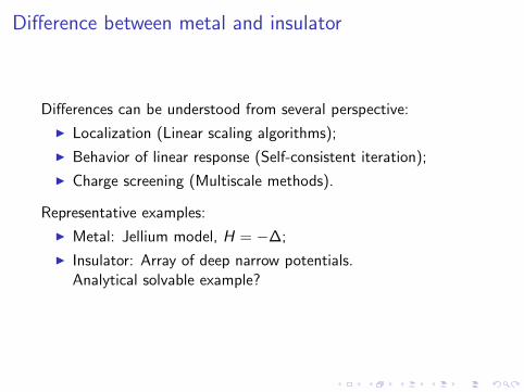
Difference between metal and insulator

Differences can be understood from several perspective:

I Localization (Linear scaling algorithms);

I Behavior of linear response (Self-consistent iteration);

I Charge screening (Multiscale methods).

Representative examples:

I Metal: Jellium model, H = −∆;

I Insulator: Array of deep narrow potentials.Analytical solvable example?

Discretization

Conventional basis sets:

I Fourier space (Plane-wave);

I Real space (Finite difference, finite element);

I Wavelet basis (multiscale).

Atomic orbital as basis functions:

I Tight binding (parametrized atomic orbital);

I Gaussian type orbitals (GTO);

I Numerical atomic orbital (NAO) [Blum et al 2009].

Mixed basis functions with atomic orbital:

I Augmented plane-wave (APW) [Slater 1937];

I Linear augmented-plane-wave (LAPW) [Andersen 1975];

I Projector augmented-wave (PAW) [Blochl 1994];

I Enriched finite element [Sukumar and Pask 2009].

Discontinuous basis functions

Representation

I Spectral decomposition:

(diag f (H[ρ]))(x) =∑n

f (En)|Ψn(x)|2.

I Fermi Operator expansion:

diag f (H[ρ]) ≈P∑

i=1

diag fi (H[ρ]),

where fi (H[ρ]) are simple (polynomials, rational functions)that the matrix function can be evaluated directly.

Evaluation

Diagonalization:

I Jacobi-Davidson Diagonalization.

I Chebyshev filtering [Zhou, Saad, Tiago et al 2006]

Fermi operator expansion:

I Polynomial expansion [Goedecker and Colombo 1994]

I Rational expansion [Baroni and Giannozzi 1992] [Lin, Lu, Yinget al 2009]

Special techniques for insulators

I Divide and Conquer [Yang 1991]

I Orbital minimization [Mauri, Galli and Car 1993]

I Density matrix minimization [Li, Nunes and Vanderbilt 1993]

I Localized subspace iteration [Garcıa-Cervera, Lu and E 2007]

I Orbital minimization with localization [E and Gao 2010]

Summary of our work

I Discretization: Discontinuous basis functions with smallnumber of basis functions per atom for chemical accuracy.

I Representation: Pole expansion for Fermi-Dirac function withoptimal representation cost.

I Evaluation: Selected inversion technique achieving O(N) forquasi-1D system, O(N1.5) for quasi-2D system, and O(N2)for 3D bulk system.

I Linear scaling algorithms for insulators:I Localized subspace iteration;I Orbital minimization with localization.

I Multiscale sublinear scaling algorithms for insulating materialswith local defects.

Fundamentals



Existing discretization methods

Uniform grid (Fourier, real space)

I Large number of basis functions per atom (500 ∼ 5000).

Atomic orbitals and mixed basis functions:

I Fine tunning of parameters.

I Different parameters for different exchange-correlationfunctional.

I Overcomplete and incomplete basis sets.

I Interstitial region.

I Basis function with large support: metallic system.

Discontinuous Galerkin framework with locally adaptivebasis

Goal: Construct local basis functions on the fly by solving a smallpart of the system.

I Local solve in a buffer to obtain basis functions adapted tothe environment;

I Discontinuous Galerkin framework to discretize the systemusing these (discontinuous) basis functions.

See Lin Lin’s talk (Thursday) for more details

DG Formulation

Minimize the DG discrete effective energy functional to get thedensity (for given effective potential):

EDG(ψi) =1

2

N∑i=1

〈∇ψi ,∇ψi 〉T +〈Veff , ρ〉T +∑`

γ`

N∑i=1

|〈b`, ψi 〉T |2

−N∑

i=1

⟨∇ψi

,[[ψi

]]⟩S +

α

h

N∑i=1

⟨[[ψi

]],[[ψi

]]⟩S .

[[u]]

= u1n1 + u2n2 on S .q

= 12 (q1 + q2) on S .

Constructing adaptive local basis function

I Buffer region associated with Ek : Qk ⊃ Ek .

I Restrict the effective Hamiltonian on Qk by assuming theperiodic boundary condition on ∂Qk and obtain Heff,Qk

.

I Take the first several eigenfunctions of Heff,Qkcalled ϕk,j,

j = 1, · · · , Jk and restrict them on Ek .

Red: Ek ; Red+Blue: Qk

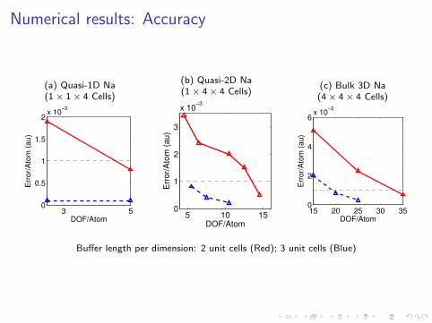
Numerical results: Accuracy

(a) Quasi-1D Na(1× 1× 4 Cells)

3 50

0.5

1

1.5

2x 10

−3

DOF/Atom

Err

or/

Ato

m (

au

)

(b) Quasi-2D Na(1× 4× 4 Cells)

5 10 150

1

2

3

x 10−3

DOF/Atom

Err

or/

Ato

m (

au)

(c) Bulk 3D Na(4× 4× 4 Cells)

15 20 25 30 350

2

4

6x 10

−3

DOF/Atom

Err

or/

Ato

m (

au)

Buffer length per dimension: 2 unit cells (Red); 3 unit cells (Blue)

Numerical results: Efficiency

128 432 1024 2000 345610

0

101

102

103

104

x2

Atom #

Wa

ll C

lock T

ime

(se

c)

Buffer Solve

DG Eigensolver

DG OverheadComputational time perprocessor comparison:

Atom# Proc# Global DGtime time

128 64 35 s 4 s432 216 248 s 35 s

Fundamentals



Fermi Operator Expansion

2

1 + eβ(H−µI )

≈

P∑

i=1

ci

(H − µI

∆E

)i

+Q∑

i=1

ωi

(zi I − (H − µI )/∆E )qi

I β inverse temperature; ∆E width of the spectrum of thediscretized Hamiltonian;

I Want P,Q, qi be as small as possible given β and ∆E .

Past work

P: Number of polynomials. Q: Number of rational functions. qi :the order of each rational function.

I P ∼ O(β∆E ),Q = 0 [Goedecker and Colombo 1994];

I P = 0, Q ∼ O(β∆E ), qi ≡ 1 [Baroni and Giannozzi 1992];

I P = 0, Q ∼ O(β∆E )1/2, qi ≡ 1 [Ozaki 2007];

I P ∼ C , Q ∼ O(β∆E )1/2, qi ≡ 1[Ceriotti, Kuhne and Parrinello 2008];

I Multipole expansion: P ∼ C , Q ∼ O(log(β∆E )), qi ∼ C[Lin, Lu, Car and E 2009];

I Pole expansion: P = 0, Q ∼ O(log(β∆E )), qi ≡ 1[Lin, Lu, Ying and E 2009].

Pole expansion

f (x) =2

1 + eβ∆Ex=

1

2πi

∮Γ

f (z)

z − xdz ≈ 1

2πi

P∑i=1

f (zi )wi

zi − x.

Optimal choice of the contour Γ, integration points zi ∈ C andintegration weights wi ∈ C → Number of discretization points∼ O(log(β∆E )).

non-analyticspectrum

1-1

Geometric convergence with small pre-constant

2D discretized Laplacian with small perturbation: energy gaparound 10−6au.

10 20 30 40 50 60 70

10−8

10−6

10−4

10−2

NPole

L1

erro

rpe

rel

ectr

on

104

105

106

60

65

70

75

80

85

90

β∆E

NPole

Fundamentals



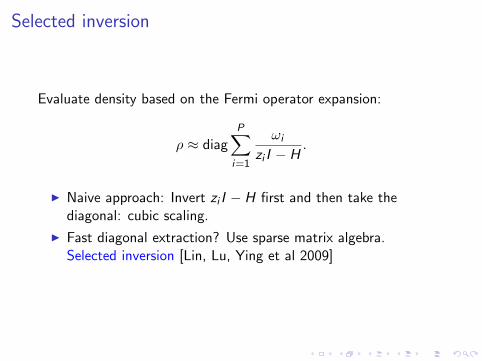
Selected inversion

Evaluate density based on the Fermi operator expansion:

ρ ≈ diagP∑

i=1

ωi

zi I − H.

I Naive approach: Invert zi I − H first and then take thediagonal: cubic scaling.

I Fast diagonal extraction? Use sparse matrix algebra.Selected inversion [Lin, Lu, Ying et al 2009]

Selected inversion: Basic idea

Gauss elimination:

A =

„α aT

a bA«

=

„1` I

«„α bA− a`T

«„1 `T

I

«,

A−1 =

„α−1 + `T S−1` −`T S−1

−S−1` S−1

«, ` = aα−1, S = bA− a`T .

If ` is sparse, computing the(1, 1) element of A−1 does notrequire all elements of S−1.

SelInv: Selected Inversion for Sparse Symmetric Matrix

SelInv is a selected inversion algorithm for general sparsesymmetric matrix written in Fortran[Lin, Yang, Meza, et al, in press]

I Symbolic Analysis: matrix reordering

I LDLT factorization

I Selected inversion

Numerical results: SelInv

Problems from Harwell-Boeing Test Collection and the Universityof Florida Matrix Collection.

problem n selected inversion direct inversion speeduptime time

bcsstk14 1,806 0.01 sec 0.13 sec 13bcsstk24 3,562 0.02 sec 0.58 sec 29bcsstk28 4,410 0.02 sec 0.88 sec 44bcsstk18 11,948 0.24 sec 5.73 sec 24bodyy6 19,366 0.09 sec 5.37 sec 60

crystm03 24,696 0.78 sec 26.89 sec 34wathen120 36,441 0.34 sec 48.34 sec 142thermal1 82,654 0.44 sec 95.06 sec 216shipsec1 140,874 17.66 sec 3346 sec 192

pwtk 217,918 14.55 sec 5135 sec 353parabolic fem 525,825 20.06 sec 7054 sec 352

tmt sym 726,713 13.98 sec > 3 hours > 772ecology2 999,999 16.04 sec > 3 hours > 673

G3 circuit 1,585,478 218.7 sec > 3 hours > 49

Parallel implementation5-pt discretization of 2D Laplacian operator:

100

101

102

103

102

103

number of processors

wal

l clo

ck ti

me

(sec

)

PSelInvideal

100

101

102

103

101

102

103

104

number of processorsG

flops

PSelInvideal

Figure: Log-log plot of total wall clock time and total Gflops with respectto number of processors, compared with ideal scaling. The largest matrixsolved has (4.3 billion)2 degrees of freedom.[Lin, Yang, Lu, et al, preprint]

Conclusion and Outlook

SummaryI Understanding the macroscopic limit of the Kohn-Sham

density functional theory, based on sharp stability conditions:I Nonlinear elasticity;I Macroscopic Maxwell equations;

I Algorithmic development for metallic systemsI Discontinuous Galerkin framework with locally adapted basis;I Fermi operator expansion with optimal scaling;I Selected inversion for sparse discrete Hamiltonian matrix;

I (not mentioned) Linear and sublinear scaling algorithms fordensity functional theory.

Density functional theory is a challenge and opportunity for appliedmathematicians. Many open questions remain on both analyticaland numerical sides.

Introduction to Kohn-Sham Density Functional Theory ... · Introduction to Kohn-Sham Density...

Documents

Transcript of Introduction to Kohn-Sham Density Functional Theory ... · Introduction to Kohn-Sham Density...