Introduction to Integrable Models - reffert.itp.unibe.ch

Introduction to Integrable Models

Lectures given at

ITP University of BernFall Term 2014

SUSANNE REFFERT

SEP./OCT. 2014

Chapter 1

Introduction and Motivation

Integrable models are exactly solvable models of many-body systems inspired from statisti-cal mechanics or solid state physics. They are usually the result of some simplifications andapproximations of a real-world physical system. As these models describe things made upof atoms, they are inherently discrete (lattice models). With some exceptions, most knownintegrable models are however one-dimensional, which means that we have quite someway to go before we can solve realistic systems. The models we can solve fully are a bit likevery simple table-top experiments. By studying these systems, we hope to gain valuabletools for tackling more complicated systems.

The concept of integrability shows up in the context of classical mechanics, classicalfield theory (e.g. classical sine–Gordon model), but also in conjunction with combinatorialobjects, such as for example triangulations, trees, tilings, alternating sign matrices, andplane partitions. Integrable models are also relevant for the high energy physicist, as theyare intimately connected to supersymmetric quantum field theories and string theory.

In these lectures, we will focus largely on one class of quantum integrable models,namely spin chains.

In 1931, Hans Bethe solved the XXX1/2 or Heisenberg spin chain. His ansatz canbe generalized to many more systems and is the basis of the field of integrable systems.Colloquially, people often equate “Bethe-solvable” with “integrable”, but the set of integrablemodels is marginally bigger.

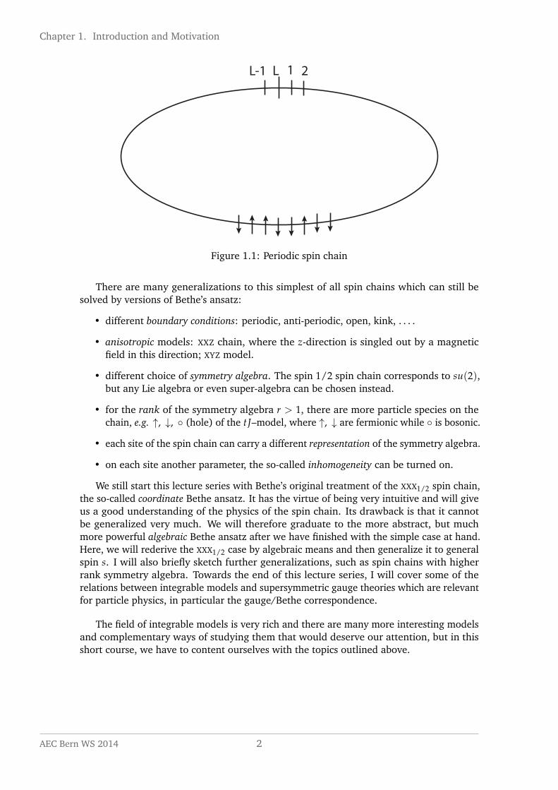
The example with which we will start our journey is the one of a 1d ferromagnet. Here,one studies a linear chain of L identical atoms with only next-neighbor interactions. Eachatom has one electron in an outer shell (all other shells being complete). These electronscan either be in the state of spin up (↑) or down (↓). At first order, the Coulomb- andmagnetic interactions result in the exchange interaction in which the states of neighboringspins are interchanged:

↑↓ ↔ ↓↑ (1.1)

In a given spin configuration of a spin chain, interactions can happen at all the anti-parallelpairs. Take for example the configuration

↑↑↓↑↓↓↓↑↑↓↓ . (1.2)

It contains five anti-parallel pairs on which the exchange interaction can act, giving rise tofive new configurations.

For simplicity, we will be studying the periodic chain. Bethe posed himself the questionof finding the spectrum and energy eigenfunctions of this spin chain. We will study his ansatzin detail in the next chapter. His method is a little gem and studying it is bound to lift themorale of any theoretical physicist!

1 AEC Bern WS 2014

Chapter 1. Introduction and Motivation

L-1 1L 2

Figure 1.1: Periodic spin chain

There are many generalizations to this simplest of all spin chains which can still besolved by versions of Bethe’s ansatz:

• different boundary conditions: periodic, anti-periodic, open, kink, . . . .

• anisotropic models: XXZ chain, where the z-direction is singled out by a magneticfield in this direction; XYZ model.

• different choice of symmetry algebra. The spin 1/2 spin chain corresponds to su(2),but any Lie algebra or even super-algebra can be chosen instead.

• for the rank of the symmetry algebra r > 1, there are more particle species on thechain, e.g. ↑, ↓, (hole) of the tJ–model, where ↑, ↓ are fermionic while is bosonic.

• each site of the spin chain can carry a different representation of the symmetry algebra.

• on each site another parameter, the so-called inhomogeneity can be turned on.

We still start this lecture series with Bethe’s original treatment of the XXX1/2 spin chain,the so-called coordinate Bethe ansatz. It has the virtue of being very intuitive and will giveus a good understanding of the physics of the spin chain. Its drawback is that it cannotbe generalized very much. We will therefore graduate to the more abstract, but muchmore powerful algebraic Bethe ansatz after we have finished with the simple case at hand.Here, we will rederive the XXX1/2 case by algebraic means and then generalize it to generalspin s. I will also briefly sketch further generalizations, such as spin chains with higherrank symmetry algebra. Towards the end of this lecture series, I will cover some of therelations between integrable models and supersymmetric gauge theories which are relevantfor particle physics, in particular the gauge/Bethe correspondence.

The field of integrable models is very rich and there are many more interesting modelsand complementary ways of studying them that would deserve our attention, but in thisshort course, we have to content ourselves with the topics outlined above.

AEC Bern WS 2014 2

Chapter 2

The coordinate Bethe ansatz

As discussed in the introduction, we want to find the energy eigenfunctions and eigenvaluesof a 1d magnet. Consider a closed chain of identical atoms with each one external electronwhich can be in the state of spin up or down and only next-neighbor interactions — theXXX1/2 spin chain. Its Hamiltonian (Heisenberg 1926) is given by

H = −JL

∑n=1

Πn,n+1, (2.1)

where J is the exchange integral1 and Πn,n+1 is the permutation operator of states atpositions n, n + 1. Let us write down the spin operator at position n on the spin chain:

~Sn = (Sxn, Sy

n, Szn) =

12~σn, (2.2)

where σn are the Pauli matrices for spin 1/2:

σ1 =

(0 11 0

), σ2 =

(0 −ii 0

), σ3 =

(1 00 −1

). (2.3)

In terms of the spin operators, the permutation operator is given by

Πn,n+1 = − 12 (1 +~σn~σn+1). (2.4)

In terms of the spin operators, the Hamiltonian (2.1) becomes

H = −JL

∑n=1

~Sn~Sn+1

= −JL

∑n=1

12

(S+

n S−n+1 + S−n S+n+1

)+ Sz

nSzn+1,

(2.5)

where S± = Sxn ± iSy

n are the spin flip operators. The term in parentheses corresponds tothe exchange interaction which exchanges neighboring spin states.

The spin flip operators act as follows on the spins:

S+k | . . . ↑ . . . 〉 = 0, S+

k | . . . ↓ . . . 〉 = | . . . ↑ . . . 〉,S−k | . . . ↑ . . . 〉 = | . . . ↓ . . . 〉, S−k | . . . ↓ . . . 〉 = 0,

Szk| . . . ↑ . . . 〉 = 1

2 | . . . ↑ . . . 〉, Szk| . . . ↓ . . . 〉 = − 1

2 | . . . ↓ . . . 〉.(2.6)

1−J > 0: ferromagnet, spins tend to align, −J < 0: anti-ferromagnet, spins tend to be anti-parallel.

3 AEC Bern WS 2014

Chapter 2. The coordinate Bethe ansatz

The spin operators have the following commutation relations:

[Szn, S±n′ ] = ±S±n δnn′ , [S+

n , S−n′ ] = 2Sznδnn′ . (2.7)

For the closed chain, the sites n and n + L are identified:

~SL+1 = ~S1. (2.8)

So far, we have discussed the isotropic spin chain. In the anisotropic case, a magnetic fieldis turned on in the z-direction:

H∆ = −JL

∑n=1

SxnSx

n+1 + SynSy

n+1 + ∆(SznSz

n+1 − 14 ). (2.9)

This is the XXZ spin chain. ∆ is the anisotropy parameter, where ∆ = 1 is the isotropic case.The most general model in this respect is the XYZ spin chain:

H∆, Γ = −L

∑n=1

JxSxnSx

n+1 + JySynSy

n+1 + JzSznSz

n+1. (2.10)

It has two anisotropy parameters ∆, Γ which fulfill the ratios

Jx : Jy : Jz = 1− Γ : 1 + Γ : ∆. (2.11)

In the following, we will however concentrate on the isotropic case.Let us define the ferromagnetic reference state

| ↑↑ . . . ↑↑〉 = |Ω〉. (2.12)

H acts on a Hilbert space of dimension 2L, given that each site on the chain can be in oneof two states, which is spanned by the orthogonal basis vectors

|Ω(n1, . . . , nN)〉 = S−n1. . . S−nN

|Ω〉, (2.13)

which are vectors with N down spins (0 ≤ N ≤ L) in the positions n1, . . . , nN, where wealways take 1 ≤ n1 < n2 < · · · < nN ≤ L.

In order to diagonalize the Heisenberg model, two symmetries will be of essentialimportance:

• the conservation of the z–component of the total spin,

[H, Sz] = 0, Sz =L

∑n=1

Szn. (2.14)

This remains also true for the XXZ spin chain Hamiltonian H∆.

• the translational symmetry, i.e. the invariance of H with respect to discrete trans-lations by any number of lattice spacings. This symmetry results from the periodicboundary conditions we have imposed.

As the exchange interaction only moves down spins around, the number of down spins ina basis vector is not changed by the action of H. Acting with H on |Ω(n1, . . . , nN)〉 thusyields a linear combination of basis vectors with N down spins. It is therefore possible toblock-diagonalize H by sorting the basis vectors by the quantum number Sz = L/2− N.

AEC Bern WS 2014 4


Let us start by considering the subsector with N = 0. It contains only one single basisvector, namely |Ω〉, which is an eigenvector of H as there are no antiparallel spins for theexchange interaction to act on:

H|Ω〉 = E0|Ω〉, E0 = −J L4 . (2.15)

Next we consider the sector with N = 1. As the down spin can be in each of the latticesites, this subspace is spanned by

|Ω(n)〉 = S−n |Ω〉. (2.16)

In order to diagonalize this block, we must invoke the translational symmetry. We canconstruct translationally invariant basis vectors as follows:

|ψ〉 = 1√L

L

∑n=1

eikn|Ω(n)〉, k =2πm

L, m = 0, 1, . . . , L− 1. (2.17)

The |ψ〉 with wave number k are eigenvectors of the translation operator with eigenvalueeik and eigenvectors of H with eigenvalues

E = −J( L4 − 1− cos k), (2.18)

or in terms of E0,E− E0 = J(1− cos k). (2.19)

The |ψ〉 are so-called magnon excitations: the ferromagnetic ground state is periodicallyperturbed by a spin wave with wave length 2π/k.

So far, we have block-diagonalized H and diagonalized the sectors N = 0, 1 by symmetryconsiderations alone. The invariant subspaces with 2 ≤ N ≤ L/2 however are notcompletely diagonalized by the translationally invariant basis.

In order to remedy this situation, we will now study Bethe’s ansatz, again for the caseN = 1.

Bethe ansatz for the one-magnon sector. We can write the eigenvectors of H in thissector as

|ψ〉 =L

∑n=1

a(n)|Ω(n)〉. (2.20)

Plugging this into the eigenvalue equation results in a set of conditions for a(n):

2[

E +JL4

]a(n) = J [2a(n)− a(n− 1)− a(n + 1)] , n = 1, 2, . . . , L. (2.21)

On top of this, we have the periodic boundary conditions

a(n + L) = a(n). (2.22)

The L linearly independent solutions to the difference equation Eq. (2.21) are given by

a(n) = eikn, k =2π

Lm, m = 0, 1, . . . , L− 1. (2.23)

Little surprisingly, these are the same solutions we had found before. But now we can applythe same procedure to the case N = 2.

5 AEC Bern WS 2014


Bethe ansatz for the two-magnon sector. This invariant subspace has dimension L(L−1)/2. We want to determine a(n1, n2) for the eigenstates of the form

|ψ〉 = ∑1≤n1<n2≤L

a(n1, n2)|Ω(n1, n2)〉. (2.24)

Bethe’s preliminary ansatz is given by

a(n1, n2) = A ei(k1n1+k2n2) + A′ ei(k1n2+k2n1). (2.25)

The first term is called the direct term and represents an incoming wave, while the secondterm is called the exchange term and represents an outgoing wave. Indeed, the expressionlooks like the superposition of two magnons, however, the flipped spins must always be indifferent lattice sites. Asymptotically, we can only have the direct and exchange terms fortwo magnons. Bethe’s ansatz postulates that this asymptotic form remains true in general.

Let us now plug the eigenstates |ψ〉 of the form given in Eq. (2.25) into the eigenvalueequation. There are two cases to consider separately, namely the two down spins not beingadjacent, and the two down spins being adjacent:

2(E− E0) a(n1, n2) = J [4 a(n1, n2)− a(n1 − 1, n2)− a(n1 + 1, n2) (2.26)

−a(n1, n2 − 1)− a(n1, n2 + 1)] , n2 > n1 + 1 ,2(E− E0) a(n1, n2) = J [2a(n1, n2)− a(n1 − 1, n2)− a(n1, n2 + 1)] , n2 = n1 + 1.

(2.27)

Equations (2.26) are satisfied by a(n1, n2) of the form Eq. (2.25) with arbitrary A, A′, k1, k2for both n2 > n1 + 1 and n2 = n1 + 1 if the energies fulfill

E− E0 = J ∑j=1,2

(1− cos k j). (2.28)

Equation (2.27) on the other hand is not automatically satisfied. Subtracting equa-tion (2.27) from equation (2.26) for the case n2 = n1 + 1 leads to L conditions, known asthe meeting conditions:

2 a(n1, n1 + 1) = a(n1, n1) + a(n1 + 1, n1 + 1). (2.29)

Clearly, the expressions a(n1, n1) have no physical meaning, as the two down spins cannotbe at the same site, but are defined formally by the ansatz Eq. (2.25). Thus the a(n1, n2)solve Eq. (2.26), (2.27) if they have the form Eq. (2.25) and fulfill Eq. (2.29). PluggingEq. (2.25) into Eq. (2.29) and taking the ratio, we arrive at

AA′

=: eiθ = − ei(k1+k2) + 1− 2 eik1

ei(k1+k2) + 1− 2 eik2. (2.30)

We see thus that as a result of the magnon interaction, we get an extra phase factor in theBethe ansatz Eq. (2.25):

a(n1, n2) = ei(k1n1+k2n2+12 θ12) + ei(k1n2+k2n1+

12 θ21), (2.31)

where θ12 = −θ21 = θ, or written in the real form,

2 cot θ/2 = cot k1/2− cot k2/2. (2.32)

k1, k2 are the momenta of the Bethe ansatz wave function. The translational invariance of|ψ〉,

a(n1, n2) = a(n2, n1 + L) (2.33)

AEC Bern WS 2014 6


is satisfied ifeik1L = eiθ , eik2L = e−iθ , (2.34)

which, after taking the logarithm, is equivalent to

L k1 = 2πλ1 + θ, L k2 = 2πλ2 + θ, (2.35)

where λi ∈ 0, 1, . . . , L− 1 are the Bethe quantum numbers which fulfill

k = k1 + k2 = 2πL (λ1 + λ2). (2.36)

We have seen that the expression for the energies, Eq. (2.28), is reminiscent of twosuperimposed magnons. The magnon interaction is reflected in the phase shift θ and thedeviation of the momenta k1, k2 from the one-magnon wave numbers. We will see thatthe magnons either scatter off each other or form bound states. In the following lectures,we will be mostly interested in the form of the Bethe equations themselves, and not somuch in their explicit solutions. But before treating the general N magnon case, we willnonetheless quickly review the properties of the Bethe eigenstates for N = 2.

We need to identify all pairs (λ1, λ2) that satisfy the Bethe Equations (2.32) and (2.35).Allowed pairs are restricted to 0 ≤ λ1 ≤ λ2 ≤ L− 1. Switching λ1 with λ2 interchanges k1and k2 and leads to the same solution. L(L + 1)/2 pairs meet the restriction, however onlyL(L− 1)/2 of them produce solutions, which corresponds to the size of the Hilbert space.There are three distinct classes of solutions:

1. One of the Bethe quantum numbers is zero: λ1 = 0, λ2 = 0, 1, . . . , L− 1. There existsa real solution for all L combinations k1 = 0, k2 = 2πλ2/L, θ = 0. These solutionshave the same dispersion relation as the one-magnon states in the subspace N = 1.

2. λ1, λ2 6= 0, λ2 − λ1 ≥ 2. There are L(L − 5)/2 + 3 such pairs and each gives asolution with real k1, k2. These solutions represent nearly free superpositions of twoone-magnon states.

3. λ1, λ2 6= 0, λ1, λ2 are either equal or differing by unity. There are 2L− 3 such pairs,but only L− 3 yield solutions. Most are complex, k1 := k/2+ iv, k2 := k/2− iv, θ :=φ + iχ. These solutions correspond to two-magnon bound states. They exhibit anenhanced probability that the two flipped spins are on neighboring sites.

The number of solutions adds up to the dimension of the Hilbert space. The first andsecond class of solutions correspond to two-magnon scattering states.

Bethe ansatz for the N–magnon sector. We are finally ready to tackle the generalcase with an unrestricted number N ≤ L of down spins. This subspace has dimensionL!/((L− N)!N!). The eigenstates have the form

|ψ〉 = ∑1≤n1<···<nN≤L

a(n1, . . . , nN)|Ω(n1, . . . , nN)〉. (2.37)

Here, we have N momenta k j and one phase angle θij = −θji for each pair (ki, k j). TheBethe ansatz now has the form

a(n1, . . . , nN) = ∑P∈SN

exp

(i

N

∑j=1

kp(j)nj +i2 ∑

i<jθp(i)p(j)

), (2.38)

7 AEC Bern WS 2014


where P ∈ SN are the N! permutations of 1, 2, . . . , N. From the eigenvalue equation, weagain get the two kinds of difference equations (the first for no adjacent down spins, thesecond for one pair of adjacent down spins),

2[E− E0] a(n1, . . . , nN) = JN

∑i=1

∑σ=±1

[a(n1, . . . , nN)− a(n1, . . . , ni+σ, . . . , nN)], (2.39)

if nj+1 > nj + 1, j = 1, . . . , N,

2[E− E0] a(n1, . . . , nN) = JN

∑i 6=jα,jα+1

∑σ=±1

[a(n1, . . . , nN)− a(n1, . . . , ni+σ, . . . , nN)] (2.40)

+ J ∑α

[2 a(n1, . . . , nN)− a(n1, . . . , njα − 1, njα+1, . . . , nN)

− a(n1, . . . , njα , njα+1 + 1, . . . , nN)],

if njα + 1 = njα+1, nj+1 > nj + 1, j 6= jα.

The coefficients a(n1, . . . , nN) are solutions of Equations (2.39), (2.40) for the energy

E− E0 = JN

∑j=1

(1− cos k j) (2.41)

if they have the form Eq. (2.38) and fulfill the N meeting conditions

2 a(n1, . . . , njα , njα + 1, . . . , nN) = a(n1, . . . , njα , njα , . . . , nN)

+ a(n1, . . . , njα + 1, njα + 1, . . . , nN), (2.42)

for α = 1, . . . , N. This relates the phase angles to the (not yet determined) k j:

eiθij = − ei(ki+k j) + 1− 2 eiki

ei(ki+k j) + 1− 2 eik j, (2.43)

or, in the real form

2 cot θij/2 = cot ki/2− cot k j/2, i, j = 1, . . . , N. (2.44)

Translational invariance, respectively the periodicity condition

a(n1, . . . , nN) = a(n2, . . . , nN , n1 + L) (2.45)

gives rise to

N

∑j=1

kp(j)nj +12 ∑

i<jθp(i)p(j) =

12 ∑

i<jθp′(i)p′(j) − 2πλp′(N) +

N

∑j=2

kp′(j−1)nj + kp′(N)(n1 + L),

(2.46)

where p′(i − 1) = p(i), i = 1, 2, . . . , N and p′(N) = p(1). All terms not involvingp′(N) = p(1) cancel, we are therefore left with N relations

L ki = 2πλi + ∑j 6=i

θij, (2.47)

with i = 1, . . . , N and λi ∈ 0, 1, . . . , L− 1. We need to again find sets of Bethe quantumnumbers (λ1, . . . , λN) which lead to solutions of the Bethe equations (2.43), (2.47). Each

AEC Bern WS 2014 8


x

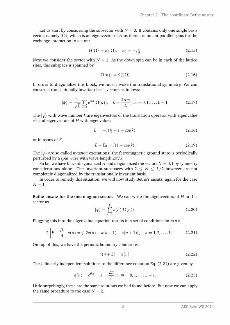
Figure 2.1: Two-body reducible chain

solution represents an eigenvector of the form Eq. (2.38) with energy (2.41) and wavenumber

k =2π

L

L

∑i=1

λi. (2.48)

Similarly to the two magnon case, bound state solutions appear, this time also with threeor more magnons.

In order to find a clear interpretation of the Bethe ansatz, let us rewrite the N–particleansatz Eq. (2.38) as follows:

a(n1, . . . , nN) = ∑P∈SN

exp

(i2 ∑

i<jθp(i)p(j)

)exp

(i

N

∑j=1

kp(j)nj

)

= ∑P∈SN

A(kp(1), . . . , kp(N)) exp

(i

N

∑j=1

kp(j)nj

).

(2.49)

The coefficient A(kp(1), . . . , kp(N)) factorizes into pair interactions:

A(kp(1), . . . , kp(N)) = ∏1≤i<j≤N

ei2 θij . (2.50)

We have seen that the two-body interactions are not free, they have a non-trivial scatteringmatrix. The many-body collisions factorize, which means they happen as a sequence of twomagnon collisions. All Bethe-solvable systems are thus two-body reducible. This propertyhas to do with the fact that a spin chain is one-dimensional, so only neighboring down spinscan interact directly (see Fig. 2.1). There are in fact very few two-dimensional systems thatare exactly solvable.

To conclude this part, we will re-write the Bethe equations to give them a form whichis more commonly used in the literature and which we will need in the last part of thislecture series. First, we introduce new variables, the so-called rapidities λi:

eik j =λj +

i2

λj − i2

. (2.51)

Plugging them into the periodicity condition, we get(λj +

i2

λj − i2

)L

=N

∏j 6=i

λi − λj + iλi − λj − i

, i = 1, . . . , N. (2.52)

This Bethe equation encodes the periodic boundary condition. In can be generalized toboundary conditions with a twist ϑ,

~SL+1 = ei2 ϑσz~S1e−

i2 ϑσz : (2.53)

9 AEC Bern WS 2014


(λj +

i2

λj − i2

)L

= eiϑN

∏j 6=i


, i = 1, . . . , N. (2.54)

The Bethe ansatz as it was presented in this lecture follows Bethe’s original treatment and isreferred to as the coordinate Bethe ansatz. It has the advantage that its physics is intuitivelyvery clear. It can be generalized to the XXZ spin chain, but not much beyond that. Theso-called algebraic Bethe ansatz is mathematically more elegant and much more powerful.It uses concepts such as the Yang–Baxter equations, the Lax operator and the R–matrix andrelies heavily on the machinery of Lie algebras and beyond. We will tackle it in the nextchapter.

As a last remark, we make the non-trivial observation that the Bethe equations (2.54)describe the critical points of a potential, the so-called Yang–Yang counting function Y. Wecan rewrite the Bethe equations as

e2πiv(λ) = 1. (2.55)

The one-form v = ∑Nj=1 vj(λ)dλj is closed and v = dY, with

Y(λ) =L

2π

N

∑i=1

x(2λi)−1

2π

N

∑i,j=1

x(λi − λj) +N

∑j=1

λj

(nj −

ϑ

2π

), (2.56)

x(λ) = λ i2

(log(1− i

λ )− log(1 + iλ ))+ 1

2 log(1 + λ2), (2.57)

where the ni are integers. The Bethe equations thus ultimately take the form

e2πdY(λ) = 1. (2.58)

The XXZ chain and SUq(2). Remember the Hamiltonian of the anisotropic XXZ spin chain,

H∆ = −JL

∑n=1

SxnSx

n+1 + SynSy

n+1 + ∆(SznSz

n+1 − 14 ). (2.59)

The anisotropy is captured by the parameter

∆ =q + 1/q

2. (2.60)

While ∆ = 1 is the isotropic case we have treated so far, the limit ∆ = ∞ corresponds tothe one-dimensional Ising model. The XXZ chain described by the Hamiltonian (2.59) canbe mapped to a two-dimensional combinatorial model, the six-vertex or ice-type model.

It was first realized by Pasquier and Saleur that the XXZ spin chain admits the groupSUq(2) (alternative notations are Uq[su(2)] and Uq(sl2)) as symmetry group. This is anexample of a quantum group, in the sense that it is a deformation by a parameter q.Quantum groups have a Hopf–algebra structure, which is also the case here.

SUq(2) is generated by S+, S− and q±SZunder the relations

qSZS±q±1S±, [S+, S−] =

q2SZ − q−2SZ

q− 1/q. (2.61)

AEC Bern WS 2014 10


These relations reduce to the ones of SU(2) for q → 1. For the case of spin 1/2, we findthe following representations for the operators:

qSZ= qσ3/2 ⊗ · · · ⊗ qσ3/2︸︷︷︸

L

, (2.62)

S± =L

∑i=1

S±i =L

∑i=1

qσ3/2 ⊗ · · · ⊗ qσ3/2︸︷︷︸i−1

⊗ σ±i /2⊗ q−σ3/2 ⊗ · · · ⊗ q−σ3/2, (2.63)

where we have the Pauli matrices

σ+ =

(0 10 0

), σ− =

(0 01 0

), σ3 =

(1 00 −1

). (2.64)

and

qσ3=

(q 00 1/q

). (2.65)

Since H∆ also commutes both with SZ and the translational operator, the Bethe ansatzworks the same as for the XXX chain.Exercise: Rederive the coordinate Bethe ansatz for H∆.

Literature. This chapter follows largely [1], which itself follows Bethe’s original work [2].The first chapter of [3] is also very useful as an introduction. The supergroup structure ofthe XXZ chain is discussed in [4].

Bibliography

[1] M. Karbach and G. Muller. Introduction to the Bethe ansatz I (1998).[2] H. Bethe. Zur Theorie der Metalle. Zeitschr. f. Phys. 71 (1931), p. 205.[3] M. Gaudin. La fonction d’onde de Bethe. Masson, Paris, 1983.[4] V. Pasquier and H. Saleur. Common Structures Between Finite Systems and Conformal Field

Theories Through Quantum Groups. Nucl.Phys. B330 (1990), p. 523.

11 AEC Bern WS 2014

Chapter 3

Introduction to the Algebraic BetheAnsatz

"Working with integrable models is a delightful pastime."

L.D. Faddeev

The algebraic Bethe ansatz (ABA) is an algebraic way of deriving the Bethe ansatzequations. It is also called the quantum inverse scattering method and was developed in thelate seventies and early eighties by the so-called Leningrad School (proponents of whichinclude Faddeev, Izergin, Korepin, Kulish, Reshetikhin, Sklyanin and Takhtajan).

We are about to uncover the mathematical reason for the integrability of the XXZ1/2spin chain, the underlying reason why Bethe’s original ansatz works. As we will see, thesu(2)–symmetry and translation invariance of the XXZ1/2 spin chain, which have alreadyproved instrumental in Bethe’s original solution, are merely the tip of the iceberg. We areabout to find an infinite dimensional symmetry (or rather L–dimensional for a finite chainof length L, which remains valid for L→ ∞).

For the time being, we will remain with our (by now) good old friend, the XXZ1/2 spinchain. Recall that we have a closed chain with L sites. Its Hilbert space has the form

H =L⊗

n=1

Hn, Hn = C2. (3.1)

For now discounting the prefactor of −J and introducing the constant −1/4 which sets thevacuum energy to zero, we write the Hamiltonian as

H =3

∑α=1

L

∑n=1

(SαnSα

n+1 − 14 ), (3.2)

where the spin operators are as before Sα = 12 σα and H fulfills [H, Sα] = 0 and Sα

n+L = Sαn.

The fundamental object of the ABA is the Lax operator, a generating object that takes itsname from the Lax operator used in the solution of the KdV equation. In order to defineit, we must introduce the auxiliary space V which for the time being is also C2, and acontinuous complex parameter λ, the spectral parameter. This parameter will allow us lateron to recover the integrals of motion as coefficients of a series expansion in λ. The auxiliaryspace V on the other hand is needed to show that the integrals of motion commute. TheLax operator acts on Hn ⊗V:

Ln,a(λ) = λ1n ⊗ 1a + i3

∑α=1

Sαn ⊗ σα, (3.3)

AEC Bern WS 2014 12

Chapter 3. The Algebraic Bethe Ansatz

where the labels n refer to Hn while the labels a refer to V. Alternatively, we can expressthe V–dependence of L explicitly by writing L as a 2× 2 matrix:

Ln,a(λ) =

(λ + i S3

n i S−ni S+

n λ− i S3n

). (3.4)

We can write Ln,a(λ) in yet another form using the fact that the operator

Π = 12 (1 +

2

∑α=1

σα ⊗ σα) (3.5)

is the permutation operator on C2 ×C2. Since Hn and V are the same,

Ln,a(λ) = (λ− i2 )1n,a + i Πn,a. (3.6)

Let us now establish the main property of the Lax operator, namely the commutationrelations for its entries. In order to take the commutator, we consider two Lax operatorsLn,a1(λ), Ln,a2(λ) acting on the same Hilbert space but different auxiliary spaces V1, V2.The product Ln,a1(λ)Ln,a2(λ) acts on the space Hn ⊗V1 ⊗V2. We now make the claim thatthere exists an operator Ra1,a2(λ− µ) in ⊗V1 ⊗V2 such that the following relation is true:

Ra1,a2(λ− µ)Ln,a1(λ)Ln,a2(µ) = Ln,a2(µ)Ln,a1(λ)Ra1,a2(λ− µ). (3.7)

This is the fundamental commutation relation (FCR) for L, it has the form of a Yang–Baxterequation (YBE). The operator R, called the R–matrix acts as an intertwiner. The explicitexpression for R is given by

Ra1,a2(λ) = λ1n,a + i Πn,a. (3.8)

We see that L and R have the same form, in fact .

Exercise: Verify Eq. (3.7) using the explicit expressions for L and R and the relation

Πn,a1 Πn,a2 = Πa1,a2 Πn,a1 = Πn,a2 Π22,a1 . (3.9)

We can also write the Yang–Baxter equation only in terms of R, which gives it a form morefamiliar from other contexts:

Ra1,a2(λ− µ)Rn,a1(λ)Rn,a2(µ) = Rn,a2(µ)Rn,a1(λ)Ra1,a2(λ− µ), (3.10)

where λ = λ + i/2, µ = µ + i/2.We can represent the YBE diagrammatically. Ln,a acts on two different types of space, so

we depict it as the crossing of two lines of different color. Ra1.a2 on the other hand acts onthe same type of space and is depicted as the crossing of two a-lines.

Ln,a =

n line

a line

Ra1.a2 =

a1

a2

The product Ln,a1(λ)Ln,a2(µ) acts on two a-lines and one n-lines:

13 AEC Bern WS 2014


Ln,a1(λ)Ln,a2(µ) =

a1

a2

n

Below, the RHS and LHS of the YBE are depicted:

a1

a2

a2

a1

n

=

a1

a2

a2

a1

n

The YBE also shows up in the context of knot theory and the braid group, where it statesthat two ways of switching the strands are equivalent. More importantly for us, the YBE

has a physical interpretation in terms of scattering processes. For a scattering matrix oftwo on-shell particles which allows only the direct (i.e. the identity) and the reflectionscattering processes, the multiple particle scattering factorizes into pairwise scatteringprocesses. If you replace R by the scattering matrix S in Eq. (3.10), it encoded the fact thatin the three-particle scattering, the order of the two-particle interactions does not matter.This is also easily read off from the diagrammatic representation. The statements "system Xis two-particle reducible" and "system X fulfills the YBE" are therefore equivalent. We haveseen in the last section that two-particle reducibility is a key property of all Bethe solvablesystems, a fact that is also encoded in the fundamental commutation relation of the Laxoperator.

The Lax operator also has a natural geometric interpretation as a connection along thespin chain. Consider the vector

ψn =

(ψ1

nψ2

n

), ψ1,2

n ∈ Hn fermion operators (3.11)

in Hn ⊗V. The Lax equation defines the parallel transport between the sites n and n + 1:

ψn+1 = Lnψn. (3.12)

The transport from n1 to n2 + 1 is given by the ordered product of Lax operators over allsites in between:

Tn2n1,a(λ) = Ln2,a(λ)Ln2−1,a(λ) . . . Ln1,a(λ). (3.13)

The full product over the entire chain is the monodromy around the circle:

TL,a(λ) = LL,a(λ)LL−1,a(λ) . . . L1,a(λ) ∈ End(H⊗V). (3.14)

TL,a(λ) describes the transport of spin around the circular chain. In the following, we willdrop the label L and write Ta when referring to the monodromy matrix.

AEC Bern WS 2014 14


Ta acts on the Hilbert space of the full chain, just as the integrals of motion. We will seein the following that it is the generating object for spin, the Hamiltonian among others. Inthe following it will be convenient to express Ta as a (2× 2) matrix in V:

Ta(λ) =

(A(λ) B(λ)C(λ) D(λ)

), A, B, C, D ∈ End(H). (3.15)

The FCR for Ta(λ) is given by

Ra1,a2(λ− µ)Ta1(λ)Ta2(µ) = Ta2(µ)Ta1(λ)Ra1,a2(λ− µ), (3.16)

which has again the form of the YBE.

Exercise: Verify the FCR for Ta(λ).

Let us now begin to extract the observables of the XXX1/2 chain from Ta(λ). Ta(λ) is apolynomial in λ of order L:

Ta(λ) = λL + iλL−1 ∑α

(Sα ⊗ σα) + . . . . (3.17)

We see that the total spin appears in the coefficient of the second highest degree. Next, wewill look for the Hamiltonian. In order to do so, we take the trace of Ta(λ) on the auxiliaryspace V:

t(λ) = Tra[Ta(λ)] = A(λ) + D(λ). (3.18)

This is the so-called transfer matrix. Via the FCR Eq. (3.16), we find that then tracescommute for different values of the spectral parameter:

[t(λ), t(µ)] = 0. (3.19)

Also t(λ) is a polynomial in λ of order L:

t(λ) = 2λL1 +L−2

∑l=0

Ql λl . (3.20)

It produces L− 1 operators Ql on H, which via the commutator of t(λ) Eq (3.19) we findto be commuting,

[Ql , Qm] = 0. (3.21)

In the following, we will make use of the fact that the point λ = 1/2 is special:

Ln,a(i/2) = i Πn,a. (3.22)

The relationd

dλLn,a(λ) = 1n,a (3.23)

holds for any λ. Therefore

Ta(i/2) = iLΠL,aΠL−1,a . . . Π1,a (3.24)

= iLΠ1,2Π2,3 . . . ΠL−1,LΠL,a. (3.25)

Taking the trace over the auxiliary space we find

t(i/2) = iLU, (3.26)

15 AEC Bern WS 2014


where we defined the shift operator

U = Π1,2Π2,3 . . . ΠL−1,L (3.27)

in H which simultaneously shifts all spins by one site and thus corresponds to the rotationof the chain by one site. Take the position variable Xn on site n:

XnU = UXn−1. (3.28)

Since the permutation operator fulfills Π∗ = Π and Π2 = 1, we have U∗U = UU∗ = 1, i.e.U is unitary. Therefore

U−1XnU = Xn−1. (3.29)

We can use U to introduce a new observable, namely the momentum P. By definition, Pproduces an infinitesimal shift. On the lattice, this translates to a shift by one lattice site:

eiP = U. (3.30)

We now proceed to expand t(λ) around λ = i/2.

ddλ

Ta(λ)∣∣λ=i/2 = iL−1 ∑

nΠL,a . . . Πn,a . . . Π1,a, (3.31)

where the hat indicates that the factor is absent. Taking the trace over V,

ddλ

t(λ)∣∣λ=i/2 = iL−1 ∑

nΠ1,2 . . . Πn−1,n+1 . . . ΠL−1,L. (3.32)

Now we multiply by t(λ)−1:

ddλ

t(λ)t(λ)−1∣∣λ=i/2 =

ddλ

ln t(λ)∣∣λ=i/2 = −i ∑

nΠn,n+1. (3.33)

As we have seen back in Eq. (2.1), we can express the Hamiltonian in terms of thepermutation operator, so we find that

H =i2

ddλ

ln t(λ)∣∣λ=i/2 −

L2

. (3.34)

We have thus seen that H is indeed part of the family of L − 1 commuting operatorsgenerated by the transfer matrix. One component of the total spin, e.g. S3, completes thisfamily to a family of L commuting operators. Since the underlying classical model has Ldegrees of freedom, this means that it is integrable.

Bethe ansatz equations for the XXX1/2 spin chain. We are now ready to connect to themain result of the last section, namely the Bethe ansatz equations. As the Hamiltonianappears as a coefficient in the expansion of the transfer matrix at λ = i/2,

t(λ) = iLU = iL−1(λ− i/2)U(2H + L) +O((λ− i/2))2, (3.35)

the eigenvalue problem for H is solved by diagonalizing t(λ) = A(λ) + D(λ). We willneed the following relations between the quantities A, B, C, D which form the matrixrepresentation of the monodromy matrix, see Eq. (3.15), which are derived from the FCR

using explicit matrix representations:

[B(λ), B(µ)] = 0, (3.36)

A(λ)B(µ) = f (λ− µ)B(µ)A(λ) + g(λ− µ)B(λ)A(µ), (3.37)

Dλ)B(µ) = h(λ− µ)B(µ)D(λ) + k(λ− µ)B(λ)D(µ), (3.38)

AEC Bern WS 2014 16


where

f (λ− µ) =λ− i

λ, g(λ− µ) =

iλ

, (3.39)

h(λ− µ) =λ + i

λ, k(λ− µ) = − i

λ. (3.40)

The full set of commutation relations is symmetric under the exchange A ↔ D, B ↔ C,which corresponds to switching all the up and down spins on the chain.

A(λ) + D(λ) has to be diagonal on the eigenstates, while C(λ) and B(λ) act as raisingand lowering operators. A crucial step is to identify a highest weight state. Such a state isthe reference state Ω with

C(λ)Ω = 0. (3.41)

Ta(λ) acting on Ω is thus upper triangular. This is true when Ln,a as given in Eq. (3.4)becomes upper triangular in Va when acting on a local state ωn ∈ Hn:

Ln(λ)ωn =

(λ + i/2 ∗

0 λ− i/2

)ωn. (3.42)

This is the case when σ+n ωn = 0, so we can identify ωn = | ↑〉, and

Ω =L⊗

n=1

ωn = | ↑ . . . ↑〉, (3.43)

just as we have seen already earlier on when studying the coordinate Bethe ansatz. Actingwith the monodromy matrix on Ω, we find

Ta(λ)Ω =

(αL(λ) ∗

0 δL(λ)

)Ω, (3.44)

with

α(λ) = λ + i/2, δ(λ) = λ− i/2. (3.45)

We see thus that Ω is an eigenstate of A(λ) and D(λ) and so also of t(λ). All othereigenvectors can be obtained from Ω by acting with the lowering operator B(λ) on it. Wewill therefore be looking for eigenvectors of level N of t(λ) of the form

Φ(λ1, . . . , λN) = B(λ1) . . . B(λN)Ω. (3.46)

Different orderings of the B(λi) lead to the same eigenstate due to Eq. (3.36). Φ(λ1, . . . , λN)is only for certain values of the λ1, . . . , λN an eigenvector of t(λ). Requiring it to be aneigenvector leads to a set of algebraic conditions on the parameters λ1, . . . , λN. We willnow act with A(λ) and D(λ) on (3.46) and use the relations (3.37) and (3.38) to commutethem through the B(λi). The result has the form(

A(λ)D(λ)

)B(λ1) . . . B(λN)Ω =

(∏N

k=1 f (λ− λk)αL(λ)

∏Nk=1 h(λ− λk)δ

L(λ)

)B(λ1) . . . B(λN)Ω

+N

∑k=1

(Mk(λ, λ)Nk(λ, λ)

)B(λ1) . . . B(λk) . . . B(λN)B(λ)Ω, (3.47)

where the first term already has the right form of an eigenvector of A(λ) and D(λ), whilewe lumped all the rest into the expressions Mk, Nk. Our goal is to find conditions on the λ

17 AEC Bern WS 2014


that will make terms of the form ∑Nk=1(Mk(λ, λ)+ Nk(λ, λ))B(λ1) . . . B(λk) . . . B(λN)B(λ)Ω

disappear. It is easy to determine M1, N1 from the relations (3.37) and (3.38), e.g.

M1(λ1, λ) = g(λ− λ1)N

∏k=2

f (λ− λ1) αL(λ1). (3.48)

From the commutation relation (3.38), we learn that we can simply substitute λ1 with anyλk, so

Mj(λ1, λ) = g(λ− λj)N

∏k 6=j

f (λj − λk) αL(λj). (3.49)

Similarly,

Nj(λ1, λ) = k(λ− λj)N

∏k 6=j

h(λj − λk) δL(λj). (3.50)

Note that g(λ− λj) = −k(λ− λj). We find that

(A(λ) + D(λ))Φ(λ) = Λ(λ, λ)Φ(λ) (3.51)

for

Λ(λ, λ) = αL(λ)N

∏j=1

f (λ− λj) + δL(λ)N

∏j=1

h(λ− λj) (3.52)

if the set λ satisfies the equation

N

∏k 6=j

f (λj − λk) αL(λj) =N

∏k 6=j

h(λj − λk) δL(λj). (3.53)

Using the explicit expressions (3.39) and (3.45), this is the Bethe equation(λj +

i2

λj − i2

)L

=N

∏j 6=k

λj − λk + iλj − λk − i

. (3.54)

In other words, we have recovered by algebraic means the exact expression of Eq. (2.52),which is naturally the way it should be, given that we have studied the same system. Theset λ is called the Bethe roots and the expression (3.46) the Bethe vector.

Let us now study the properties of the eigenvectors (3.46), such as their spin, momentumand energy.

Spin. Taking µ→ ∞ in the YBE (3.7) and representing the monodromy in terms of spinoperators using Eq. (3.3), we find

[Ta(λ), 12 σα + Sα] = 0, (3.55)

which expresses the su(2) invariance of Ta(λ) in H⊗V. In particular, we have

[S3, B] = −B, [S+, B] = A− D. (3.56)

We know that for the reference state Ω,

S+Ω = −0, S3Ω = L2 Ω. (3.57)

AEC Bern WS 2014 18


Ω is thus a highest weight state for the spin operator Sα. Applying the relations Eq. (3.56)to the Bethe vectors, we find

S3Φ(λ) = ( L2 − N)Φ(λ), (3.58)

S+Φ(λ) = ∑j

B(λ1) . . . B(λj−1)(A(λj)− D(λj))B(λj+1) . . . B(λN)Ω (3.59)

= ∑k

Ok(λ)B(λ1) . . . B(λk) . . . B(λj+1) . . . B(λN)Ω. (3.60)

Along the same lines as we have derived the Bethe equations, one can show that thecoefficients Ok all vanish if the λ fulfill the Bethe equations (3.54). The Bethe vectorsare thus all highest weight states of the spin operator.

Since the S3 eigenvalue of the highest weight state must be non-negative, we must haveN ≤ L/2. The spectrum of H is degenerate under the exchange of all spin up and spindown states, so effectively the whole range is covered.

Momentum. Recall that t(i/2) = iLU. Using Eq. (3.52), we find

Λ(i/2, λ) = iLN

∏j=1

λj + i/2λj − i/2

. (3.61)

Taking the logarithm for the momentum,

P Φ(λ) = −iN

∑j=1

lnλj + i/2λj − i/2

Φ(λ), (3.62)

where we can define

p(λj) = −i lnλj + i/2λj − i/2

. (3.63)

We see that the momentum is additive and that each λj has momentum p(λj).

Energy. The same is true for the energy. Using the expression for H we found in Eq. (3.34),we find

H Φ(λ) =N

∑j=1

ε(λj)Φ(λ), (3.64)

withε(λj) = −

12

1λ2 + 1/4

. (3.65)

We see thus that it makes sense to use a quasiparticle interpretation for the spectrum ofobservables on the Bethe vectors. Each quasiparticle is created by B(λ), diminishes the spinS3 by one, has momentum p(λ) and energy ε(λ). Of course these are again the magnonswe have encountered in the discussion of Bethe’s original results. As we have the relation

ε(λ) = −12

ddλ

p(λ), (3.66)

the λ can be interpreted as the rapidity of the quasiparticle.The Hamiltonian in Eq. (3.2) corresponds, unlike the case we studied in the last section,

to the anti-ferromagnetic case, where Ω is not the ground state. If we take instead −H, weare back in the ferromagnetic case, as before.

We have thus come to a full circle, having recovered by algebraic means all the physicalproperties of the XXX1/2 chain we had studied via the more physically transparent coordinateBethe ansatz.

19 AEC Bern WS 2014


Literature. This chapter largely follows lecture notes of Faddeev [1], with some extrapadding here and there.

Bibliography

[1] L. D. Faddeev. “How algebraic Bethe Ansatz works for integrable model”. In: QuantumSymmetries / Symmetries Quantiques. Ed. by A. C. et al. North-Holland, Amsterdam, 1998,pp. 149–219.

AEC Bern WS 2014 20

Chapter 4. General Spin Chains

Chapter 4

General Spin Chains via theAlgebraic Bethe Ansatz

One of the main arguments for preferring the algebraic Bethe ansatz over the original oneis that it is applicable to a range of more general spin chains. We will study in the followingtwo generalizations.

The XXXs Chain. One obvious generalization is to study the XXX model, but for generalspin s. Here, the Hilbert space is H = C2s+1. Naively, one is tempted to just rewrite theHamiltonian Eq. (3.2),

H =3

∑α=1

L

∑n=1

(SαnSα

n+1 − 14 ), (4.1)

where we take Sαn to be in the representation of spin s. The problem with this naive

approach is, that the Hamiltonian (4.1) is not integrable!Armed with the knowledge of the last section, we try instead via the ABA. The first

naive attempt involves constructing a Lax operator on Hn ⊗V = C2s+1 ⊗C2. To a certaindegree, this works, as the derivation of the BAE works along the same lines as before: theLax operator

Ln,a(λ) =

(λ + i S3

n i S−ni S+

n λ− i S3n

)(4.2)

satisfies the YBE (3.7) with the same R–matrix as before, Ra1,a2(λ) = La1,a2(λ + i/2). Wecan define the monodromy and the reference vector Ω =

⊗ωn, where ωn is now the

highest weight state in C2s+1. Also the Bethe vectors are formally the same as before, andwe find the BAE for the roots λ,(

λj + isλj − is

)L

=N

∏j 6=k

λj − λk + iλj − λk − i

. (4.3)

This is a natural and obvious generalization of Eq. (3.54). The generalization of theargument to extract H from t however does not work, as we cannot express the Laxoperator via a permutation operator as in Eq. (3.6), since now Hn and V are not the same.We must therefore adopt a more general approach and construct a Lax operator for Hn andV isomorphic.

Take an abstract algebra A, which is defined via the ternary relation on A⊗A⊗A

R12R13R23 = R23R13R12, (4.4)

21 AEC Bern WS 2014


where R is a universal R–matrix acting on A⊗A and the labels indicate on which of thethree factors of A⊗A⊗A R acts:

R12 = R⊗ 1, R23 = 1⊗R, (4.5)

etc. A has a family of representations ρ(a, λ) parametrized by a discrete label a and acontinuous label λ. For the XXX model, A is the so-called Yangian, named by Drinfeld afterC.N. Yang. The Yangian is another example of a quantum group, it has the structure ofan infinite-dimensional Hopf algebra. Most generally speaking, it is a deformation of theuniversal enveloping algebra U(a[z]) of the semi-simple Lie algebra of polynomial loops ofthe semi-simple Lie algebra a. We will however not work at this level of generality. Thedefinition via the YBE (4.4) works for the Lie algebra a = gl(n) and is thus sufficient forour needs.

Concretely, we can obtain the Lax operators via the evaluation representation of theuniversal R-matrix:

Ln,a(λ, µ) = (ρ(a, λ)⊗ ρ(n, µ))R = Ra,n(λ− µ), (4.6)

where ρ(a, λ) is a representation of the Yangian of su(2) and the discrete label a =0, 1/2, 1, . . . is the spin label. We can recover our original YBE Eq. (3.7) for spin 1/2 fromEq. (4.4) by applying the representations ρ(1/2, λ)⊗ ρ(1/2, µ)⊗ ρ(s, σ), setting σ = 0 andmaking the identifications

Ra1,a2(λ) = R1/2,1/2(λ), Ln,a1(λ) = R1/2,s(λ). (4.7)

In order to study the general case of spin s, it is most convenient to cast the YBE Eq. (4.4)via permutations into the form

R12R32R31 = R31R32R12. (4.8)

To this YBE, we apply the representation ρ(s1, λ)⊗ ρ(s2, µ)⊗ ρ(1/2, σ), where s1 labels thelocal Hilbert space Hn and s2 labels the auxiliary space V. This leads to the relation

Rs1,s2(λ− µ)R1/2,s2(σ− µ)R1/2,s1(σ− λ) = R1/2,s1(σ− λ)R1/2,s2(σ− µ)Rs1,s2(λ− µ).(4.9)

For the case we are interested in where Hn and V have equal dimension, namely s1 = s2,we can construct a new fundamental Lax operator Ln, f (λ) from the YBE above. To do so,let us denote the two sets of spin operators labeled by s1 and s2 by Sα and Tα, and theirLax operators as

LS(λ) = λ + i (S, σ), LT(λ) = λ + i (T, σ), (4.10)

where (S, σ) = ∑α Sασα and likewise for T, along the lines of the spin 1/2 case. We willsearch for Rs1,s2(λ) of the form

Rs1,s2(λ) = Πs1,s2r((S, T), λ), (4.11)

where Πs1,s2 is the permutation operator in C2s+1 ⊗C2s+1, Π(S, σ)Π = (T, σ), and r is anoperator which depends on the Casimir

C = (S, T) = ∑α

SαTα (4.12)

and λ. Plugging LS, LT and Rs1,s2 into Eq. (4.9), we can rewrite it as

(λ− i(T, σ))(µ− i(S, σ))r(λ− µ) = r(λ− µ)(µ− i(T, σ))(λ− i(S, σ)). (4.13)

AEC Bern WS 2014 22


Using the property of the Pauli matrices

(T, σ)(S, σ) = (T, S) + i((S× T), σ), (4.14)

where (S× T)α = εαβγSβTγ, and the fact that the Casimir commutes with everything, wecan turn Eq. (4.14) into

(λSα + (S× T)α)r(λ) = r(λ)(λTα + (S× T)α). (4.15)

It is enough to consider one out of the three equations above, e.g. the combination

(λS+ + i(T3S+ − S3T+))r(λ) = r(λ)(λT+ + i(T3S+ − S3T+)). (4.16)

We will switch to the variable J instead of (S, T) and use the irreducibility of the represen-tations of S and T:

(S + T)2 = S2 + T2 + 2(S, T) = 2s(s + 1) + 2(S, T) = J(J + 1), (4.17)

where J has eigenvalue j in each irreducible representation Dj in the Clebsch-Gordandecomposition

Ds ⊗ Ds =2s

∑j=0

Dj. (4.18)

Remember that we are doing all of this to find an operator r in order to construct Rs1,s2

in the form Eq. (4.11). To find r as a function of J, we use Eq. (4.16) in the subspace ofhighest weights in each Dj, i.e

T+ + S+ = 0. (4.19)

We can do this because[T3S+ − S3T+, T+ + S+] = 0, (4.20)

which means that the combination T3S+ − S3T+ appearing in Eq. (4.16) does not take youout of the subspace of highest weights. In this subspace, J = S3 + T3, so Eq. (4.16) reducesto

(λS+ + i JS+)r(λ, J) = r(λ, J)(−λS+ + i JS+). (4.21)

Using S+ J = (J − 1)S+, we find

(λ + i J)r(λ, J − 1) = r(λ, J)(−λ + i JS), (4.22)

which is a functional equation for r(λ, J). It is solved by

r(λ, J) =Γ(J + 1 + iλ)Γ(J + 1− iλ)

, (4.23)

where the Γ–function appears (remember Γ(n + 1) = n!). It is normalized such thatr(0, J) = 1 and r(−λ, J)r(λ, J) = 1. In the case we are interested in, J = 0, 1, . . . , 2s, but inprinciple r(λ, J) can be used in all generality with s ∈ C. After all of this, we can now plugEq. (4.23) into Eq. (4.11) and rewrite the FCR as

R f1, f2(λ− µ)Ln, f1(λ)Ln, f2(µ) = Ln, f2(µ)Ln, f1(λ)R f1, f2(λ− µ). (4.24)

We finally have an expression where the auxiliary spaces V1, V2 are isomorphic to the localHilbert space Hn = C2s+1. From here on, we can now reproduce the reasoning used forthe case s = 1/2. We can define the momodromy

Tf (λ) = LL, f (λ)LL−1, f (λ) . . . L1, f (λ) (4.25)

23 AEC Bern WS 2014


and the transfer matrixt f (λ) = Tr f Tf (λ). (4.26)

We find again[t f (λ), t f (µ)] = 0. (4.27)

Using Eq. (4.4) with s1 = s2 = s, R1/2,s(λ− µ) as R–matrix and R1/2,s(µ), Rs,s(λ) as Laxoperators, we find commutativity also for the families t f (λ) and ta(λ):

[t f (λ), ta(µ)] = 0. (4.28)

To derive the BAE, we use ta(λ) (i.e the case s = 1/2), while for the observables, we uset f (λ):

t f (0) = U = eiP, (4.29)

H = id

dλln t f (λ)|λ=0 =

L

∑n=1

Hn,n+1, (4.30)

Hn,n+1 = id

dλln r(J, λ)|λ=0, (4.31)

where J is constructed via the local spins Sαn, Sα

n+1:

J(J + 1) = 2 ∑α

(SαnSα

n+1) + 2s(s + 1). (4.32)

We get thusHn,n+1 = −2ψ(J + 1), (4.33)

where ψ is the logarithmic derivative of the Γ–function. For n ∈N, ψ(1+ n) = ∑Nk=1

1k − γ,

where γ is the Euler constant. Hn,n+1 can be expressed in terms of a polynomial inCn,n+1 = ∑α Sα

nSαn+1:

Hn,n+1 =2s

∑j=1

ck(Cn,n+1)k = f2s(Cn,n+1), with (4.34)

f2s(x) =2s

∑j=1

(j

∑k=1

1k− γ

)2s

∏l=0

x− xl

xj − xl, where (4.35)

xl =12 (l(l + 1)− 2s(s + 1)). (4.36)

Let us write this down explicitly for the case of s = 1. Here, c1 = −c2, so

H = ∑α,n

(SαnSα

n+1 − (SαnSα

n+1)2). (4.37)

This generalization from the spin 1/2 Hamiltonian one could not have easily guessed!Last, we give the eigenvalues of the fundamental transfer matrix t f (λ) on the Bethe vectorΦ(λ):

Λ f (λ, λ) =s

∑−s

αm(λ)L

l

∏k=1

cm(λ− λk). (4.38)

To extract the energy and the momentum of the quasiparticles, it is enough to knowαm(0) = 0, m = −s,−s + 1, . . . , s− 1,αs(0) = 1,

(4.39)

AEC Bern WS 2014 24


andcs(λ) =

λ− isλ + is

. (4.40)

With this, we get

p(λ) = −i lnλ− isλ + is

, ε(λ) = − sλ2 + s2 and (4.41)

ε(λ) = −12

ddλ

p(λ). (4.42)

We see that the energy and momentum of the magnon generalize in a straightforwardway from the case of spin 1/2, while this is not at all the case for the Hamiltonian. Thegeneralization of the xxx spin chain to spin s is one of the important achievements of theABA.

Spin chains with higher rank symmetry algebra. Another obvious way in which thexxx spin chain can be generalized is by choosing a symmetry algebra with rank r > 1, e.g.gl(n), where r = n− 1. In this case, the nested Bethe ansatz (Kulish, Resetikhin) must beapplied. It works by reducing the rank r case to the one of rank r− 1, and so on, until wearrive again at rank one. Given the time constraints of this lecture series, I will merelysketch the method to give the reader a general idea of how it works.

For each of the r− 1 steps, a new monodromy and transfer matrix are constructed. Inthe first step, we decompose T(λ) as

T(λ) =(

t11(λ) B(1)(λ)

C(1)(λ) T(2)(λ)

)∈ End(Cr), (4.43)

where B(1) is a row vector in Cr, C(1) is a column vector in Cr, and T(2)(λ) is a matrix inEnd(Cr−1). T(2)(λ) gets decomposed in the same way in the next step. Each step givesrise to a separate Bethe vector and a set of rapidities λ

(a)j j = 1, . . . , Na a = 1, . . . , r. We

start with an Ar chain with L sites, where N1 is the number of pseudo-excitations. Inthe next step, we get an Ar−1 with L + N1 sites. The additional N1 sites correspond tofundamental representations of Ar−1. Now we need to find the eigenvectors of the Ar−1 bydiagonalizing the new transfer matrix. A new highest weight state needs to be identified,etc. This leads now to an Ar−2 chain with L + N1 + N2 sites, and so on. The rank r chaindiffers from the case we have studied so far in that

• it has r different particle species, with particle numbers N1, . . . , Nr.

• for each species a, there is an effective length of the chain La, a = 1, . . . , r.

• each particle species has its own set of rapidities λ(a)j

• each particle species has its own twist parameter ϑ(a) for the boundary conditions.

The simple spin chain interpretation we had for the rank one case thus gets somewhatstretched by this generalization.

Let us end by giving the nested Bethe equations:

La

∏n=1

λi + is(a)n

λi − is(a)n

= eiϑ(a)r

∏b=1

Na

∏j=1

(i,a) 6=(j,b)

λ(a)i − λ

(b)j + i

2 Cab

λ(a)i − λ

(b)j −

i2 Cab

, (4.44)

where i = 1, . . . , Na, the spin operators are realized as generators of Ar and Cab is theCartan matrix of Ar.

25 AEC Bern WS 2014


Literature. This chapter largely follows lecture notes of Faddeev [1]. The nested Betheansatz was first discussed in [2].

Bibliography

[1] L. D. Faddeev. “How algebraic Bethe Ansatz works for integrable model”. In: QuantumSymmetries / Symmetries Quantiques. Ed. by A. C. et al. North-Holland, Amsterdam, 1998,pp. 149–219.

[2] P. Kulish and N. Y. Reshetikhin. DIAGONALIZATION OF GL(N) INVARIANT TRANSFER MATRI-CES AND QUANTUM N WAVE SYSTEM (LEE MODEL). J.Phys. A16 (1983), pp. L591–L596.

AEC Bern WS 2014 26

Chapter 5

Relations between Spin Chains andSupersymmetric Gauge Theories

Gauge theories are the foundation of our understanding of nature. Of the fundamentalinteractions, the electroweak force and QCD (strong interaction) are described by quantumgauge theories. Understanding gauge theories as well as possible is a top priority. Despitedecades of research, there are still open problems remaining, in particular regarding theirnon-perturbative behavior and confinement. One way of rendering quantum gauge theoriesmore tractable is to introduce supersymmetry. We will be using supersymmetry as a tool togain insights into gauge theories, as a kind of laboratory for studying them. Supersymmetryconstrains a theory and makes it well-behaved. It has a number of desirable mathematicalproperties, such as e.g. non-renormalisation theorems and protection of certain quantitiesfrom quantum corrections. The more supersymmetry a theory has, the more constrained itis, but a the same time, the less realistic it is from a phenomenological point of view (e.g.N = 4 super Yang–Mills theory).

In recent years, N = 2 gauge theories have been a focus of interest. Seiberg and Witten(1994) showed that N = 2 SYM theory can be solved completely at the quantum level. It ispossible to construct an exact low energy Lagrangian and the exact spectrum of BPS states.It displays moreover a strong/weak duality and has a rich algebraic structure survivingquantum corrections.

In the following, we will be particularly interested in deformations of supersymmetricgauge theories that preserve some of the supersymmetry and in particular preserve itsuseful properties. There will be two types of deformation of relevance:

• mass deformations (e.g. twisted mass deformations in 2D).

• Ω–type deformations.

In the Ω–deformation, deformation parameters εi are introduced which break Poincarésymmetry. It was introduced by Nekrasov (2004) as a calculational device for a localizationcalculation of the instanton sum of N = 2 SYM. However, it is also interesting to studyΩ–deformed gauge theories in their own right.

We will see in the following that these deformed gauge theories are intimately connectedwith integrable systems.

The relations between integrable models and supersymmetric gauge theories are avery interesting subject and active research topic. There are several examples of theseconnections, e.g.

• 2d gauge/Bethe correspondence: N = (2, 2) gauge theories in 2d are related toBethe-solvable spin chains.

27 AEC Bern WS 2014

Chapter 5. Spin Chains and Supersymmetric Gauge Theories

• 4d gauge/Bethe correspondence: Ω–deformed N = 2 supersymmetric gauge theoriesare related to quantum integrable models.

• Alday–Gaiotto-Tachikawa (AGT) correspondence: Ω–deformed super Yang–Mills theoryin 4d is related to Liouville theory.

In these lectures, we will concentrate on the 2d gauge/Bethe correspondence (Nekrasov–Shatashvili). We will match the parameters of a spin chain to those of N = (2, 2) su-persymmetric gauge theories. It will turn out that the full (Bethe) spectrum of the spinchain corresponds one-to-one to the supersymmetric ground states of the correspondinggauge theories. We have acquired the necessary knowledge on the spin chain side of thecorrespondence:

Spin Chain:

• parameters of a general spinchain

• Bethe ansatz equations

• Yang–Yang countingfunction

Supersymmetric gauge theories:

• N = (2, 2) gauge theories

• twisted mass deformation

• low energy effective action, in particularthe effective twisted superpotential

• equation for the ground states

Before we can discuss the relations between the two sides, we need to familiarizeourselves with the necessary concepts in 2d supersymmetric gauge theory. In order to doso, we follow closely sections 12.1, 12.2, 15.2 and 15.5 of the book Mirror Symmetry byK. Hori et al [1].1

Gauge/Bethe correspondence for the XXX1/2 spin chain. Recall the Bethe ansatz equa-tion for the N–magnon sector, Eq. (2.52):(

λi +i2

λi − i2

)L

=N

∏j=1j 6=i


, i = 1, . . . , N . (5.1)

We have seen that it is expressed equivalently by

e2πdY(λ) = 1, (5.2)

where Y us the Yang–Yang function, given explicitly by

Y(λ) =L

2π

N

∑i=1

(λi − i/2)(log(λi − i/2)− 1)− (λi + i/2)(log(−λi − i/2)− 1)

− 12π

N

∑i,j=1

(λi − λj + i)(log(λi − λj + i)− 1) +N

∑j=1

λj

(nj −

ϑ

2π

).

(5.3)

This result we now want to compare with the N = (2, 2) gauge theory with gauge groupU(N), one adjoint mass madj and L fundamental and anti-fundamental fields Qi, Qi with

1This actually takes a good two lectures to cover, but as I cannot really improve on the book, I see little gainin re-typing the material here.

AEC Bern WS 2014 28


E

N0 1 2 3 4

S+

S−

SU(2)multiplet

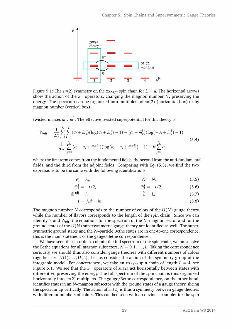
gaugetheory

Figure 5.1: The su(2) symmetry on the XXX1/2 spin chain for L = 4. The horizontal arrowsshow the action of the S± operators, changing the magnon number N, preserving theenergy. The spectrum can be organized into multiplets of su(2) (horizontal box) or bymagnon number (vertical box).

twisted masses mf, mf. The effective twisted superpotential for this theory is

Weff =1

2π

N

∑i=1

L

∑k=1

(σi + mfk)(log(σi + mf

k)− 1)− (σi + mfk)(log(−σi + mf

k)− 1)

− 12π

N

∑i,j=1

(σi − σj + madj)(log(σi − σj + madj)− 1)− itN

∑j=1

σj,

(5.4)

where the first term comes from the fundamental fields, the second from the anti-fundamentalfields, and the third from the adjoint fields. Comparing with Eq. (5.3), we find the twoexpressions to be the same with the following identifications:

σi = λi, N = N, (5.5)

mfk = −i/2, mf

k = −i/2 (5.6)

madj = i, L = L, (5.7)

t = 12π ϑ + in. (5.8)

The magnon number N corresponds to the number of colors of the U(N) gauge theory,while the number of flavors corresponds to the length of the spin chain. Since we canidentify Y and Weff, the equations for the spectrum of the N–magnon sector and for theground states of the U(N) supersymmetric gauge theory are identified as well. The super-symmetric ground states and the N–particle Bethe states are in one-to-one correspondence,this is the main statement of the gauge/Bethe correspondence..

We have seen that in order to obtain the full spectrum of the spin chain, we must solvethe Bethe equations for all magnon subsectors, N = 0, 1, . . . , L. Taking the correspondenceseriously, we should thus also consider gauge theories with different numbers of colorstogether, i.e. U(1), . . . , U(L). Let us consider the action of the symmetry group of theintegrable model. For concreteness, we take an XXX1/2 spin chain of length L = 4, seeFigure 5.1. We see that the S± operators of su(2) act horizontally between states withdifferent N, preserving the energy. The full spectrum of the spin chain is thus organizedhorizontally into su(2) multiplets. The gauge/Bethe correspondence, on the other hand,identifies states in an N–magnon subsector with the ground states of a gauge theory, slicingthe spectrum up vertically. The action of su(2) is thus a symmetry between gauge theorieswith different numbers of colors. This can bee seen with an obvious example: for the spin

29 AEC Bern WS 2014


U(La) U(Lb)

U(Na) U(Nb)i2 Λa

k ± ν(a)k

i2 Λb

k ± ν(b)k

i2 Caa

i2 Cab

i2 Cba

i2 Cbb

Qak, Qa

k

Φa

Bab

Bba

Figure 5.2: Example quiver diagram for the Gauge/Bethe correspondence. Gauge groupsare labeled in black, matter fields in blue, the corresponding twisted masses in red.

chain, the physics is the same if we use the reference state |Ω〉 = | ↑ . . . ↑〉 or instead| ↓ . . . ↓〉. The sector with N down spins starting with |Ω〉 and the one with L− N up spinsstarting from the reference state | ↓ . . . ↓〉 are the same. The spectrum of the spin chain hastherefore a manifest N, L− N symmetry. This equivalence is reflected on the gauge theoryside as the Grassmannian duality. The vacuum manifold of the low energy effective gaugetheory corresponding to the XXX1/2 chain is the cotangent bundle of the GrassmannianT∗Gr(N, L), where the Grassmannian is the collection of all linear subspaces of dimensionN of a vector space of dimension L:

Gr(N, L) = W ⊂ CL|dim W = N, (5.9)

T∗Gr(N, L) = (X, W), W ∈ Gr(N, L), X ∈ End(CL)|X(CL) ⊂W, X(W) = 0. (5.10)

The Grassmannian duality states that there is an isomorphism between Gr(N, L) andGr(L− N, L), thus linking the ground states of the low energy U(N) and U(L− N) gaugetheories.

The integrable structure of the spin chain remains hidden on the gauge theory sideof the correspondence as long as the gauge theories with different numbers of colors areconsidered separately. A mathematical framework that unifies these gauge theories in ameaningful way is Ginzburg’s geometric representation theory.

We have studied only the simplest example of the correspondence involving the XXX1/2spin chain, but the scope of the gauge/Bethe correspondence is much larger. So let us havea quick look at the general dictionary between gauge theory and spin chain parameters,see Table 5.1.

In general, we are dealing with a quiver gauge theory, which can be summarized by agraph, see Fig. 5.2. The black nodes represent gauge groups, arrows between the nodescorrespond to bifundamental fields, arrows from a node to itself indicate adjoint fields,white nodes represent flavor groups and the dashed arrows between flavor and gaugenodes represent fundamental and anti-fundamental fields.

Using Table 5.1, the values of the twisted masses that we recovered from the correspon-dence can be traced back to the Cartan matrix of su(2),

Cab =

(2 −1

−1 2

), (5.11)

the fact that we had the fundamental representation at every site, so Λk = 1, and theabsence of inhomogeneities.

AEC Bern WS 2014 30


gauge theory integrable model

number of nodes in thequiver

r r rank of the symmetry group

gauge group at a–th node U(Na) Na number of particles of species a

effective twistedsuperpotential

Weff(σ) Y(λ) Yang–Yang function

equation for the vacua e2π d Weff = 1 e2πi d Y = 1 Bethe ansatz equation

flavor group at node a U(La) La effective length for the species a

lowest component of thetwisted chiral superfield

σ(a)i λ

(a)i rapidity

twisted mass of thefundamental field

mf(a)k

i2 Λa

k + ν(a)k

highest weight of the representa-tion and inhomogeneity

twisted mass of theanti–fundamental field

mf(a)k

i2 Λa

k − ν(a)k

highest weight of the representa-tion and inhomogeneity

twisted mass of the adjointfield

madj(a) i2 Caa diagonal element of the Cartan

matrix

twisted mass of thebifundamental field

mb(ab) i2 Cab non–diagonal element of the Car-

tan matrix

FI–term for U(1)–factor ofgauge group U(Na)

τa ϑa boundary twist parameter forparticle species a

Table 5.1: Dictionary in the Gauge/Bethe correspondence.

31 AEC Bern WS 2014


Literature. The gauge theory prerequisites are explained in sections 12.1, 12.2, 15.2 and15.5 of the book Mirror Symmetry by K. Hori et al [1].

The 2d gauge/Bethe correspondence was introduced in [2, 3]. The dictionary isexplained in detail in [4, 5].

Bibliography

[1] K. Hori et al. Mirror Symmetry. Clay Mathematics Monographs 1. American MathematicalSociety, Clay Mathematics Institute, 2003.

[2] N. A. Nekrasov and S. L. Shatashvili. Supersymmetric vacua and Bethe ansatz. Nucl. Phys. Proc.Suppl. 192-193 (2009), pp. 91–112.

[3] N. A. Nekrasov and S. L. Shatashvili. Quantum integrability and supersymmetric vacua. Prog.Theor. Phys. Suppl. 177 (2009), pp. 105–119.

[4] D. Orlando and S. Reffert. Relating Gauge Theories via Gauge/Bethe Correspondence. JHEP 1010(2010), p. 071.

[5] D. Orlando and S. Reffert. Twisted Masses and Enhanced Symmetries: the A&D Series. JHEP 02(2012), p. 060.

AEC Bern WS 2014 32

Introduction to Integrable Models - reffert.itp.unibe.ch

Documents

Transcript of Introduction to Integrable Models - reffert.itp.unibe.ch