Introduction to inferentialstatistics

Alissa MelingerIGK summer school 2006

Edinburgh

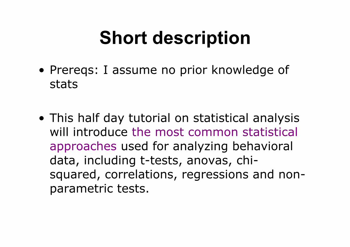
Short description• Prereqs: I assume no prior knowledge of

stats

• This half day tutorial on statistical analysiswill introduce the most common statisticalapproaches used for analyzing behavioraldata, including t-tests, anovas, chi-squared, correlations, regressions and non-parametric tests.

• The focus will be on the appropriateapplication of these methods (when to usewhich test) rather than on their underlyingmathematical foundations. The introductionwill be presented in a very pragmaticproblem-oriented manner with examples ofhow to conduct the analyses using SPSS,interpret the program output and reportthe results. One goal of the tutorial will beto generalize the use of these tests …

• Won’t learn how to conduct the analyses, buthopefully enough background to help youbootstrap up (with help from r-tutorial or Dr.Google)

Structure of Tutorial

• Hour 1: Background and fundamentalunderpinnings to inferential statistics

• Hour 2: Tests for evaluating differences

• Hour 3: Tests for evaluating relationsbetween two (or more) variables

Background and fundamentalunderpinnings to inferential

statisticsHour 1

The Experiment

• An experiment should allow for asystematic observation of a particularbehavior under controlled circumstances.

• If we properly control the experiment,there should be minimal differencebetween the situations we create.

• Therefore any observed quantitative orqualitative difference must be due to ourmanipulation.

Two Types of Variables

• You manipulate the situations under whichthe behavior is observed and measured.The variables you manipulate are yourindependent variables.

• You observe and measure a particularbehavior. This measurement is yourdependent variable

Two Types of Variables

• The independent variable is the variablethat will be manipulated and compared orthat conditions or governs the behavior.– Word length, sentence type, frequency,

semantic relationship, instruction types, age,sex, task, etc.

• The dependent variable is the behaviorthat will be observed and measured.– Reaction times, accuracy, weight, ratings, etc.

IV Terminology

• Factor is another word for independentvariable, e.g., word frequency or length

• Level- value or state of the factor.• Condition (treatments)- all the different

situations you create by combining thelevels of your different factors.

IV Terminology: Example

• Question: Does the frequency of anantecedent influence the ease ofprocessing an anaphor?– IV (factor) 1 Antecedent frequency with two

levels (frequent vs. infrequent)• Alone, this would produce two conditions

– IV (factor) 2 Anaphor type with two levels(repeated NP vs. Pronoun)

Combining levels factorially

Condition 4Pronoun - frequent antecedent

Condition 3Pronoun - infrequent antecedent

Condition 2Repeated NP - frequent antecedent

Condition 1Repeated NP - infrequent antecedent

• Each level of each factor is combined with eachlevel of each other factor, we get 4 conditions

• 2 levels x 2 levels = 4 conditions• 2 levels x 3 levels = 6 conditions

How to choose a stat• 3 issues determine what statistical test is

appropriate for you and your data:

– What type of design do you have?

– What type of question do you want to ask?

– What type of data do you have?

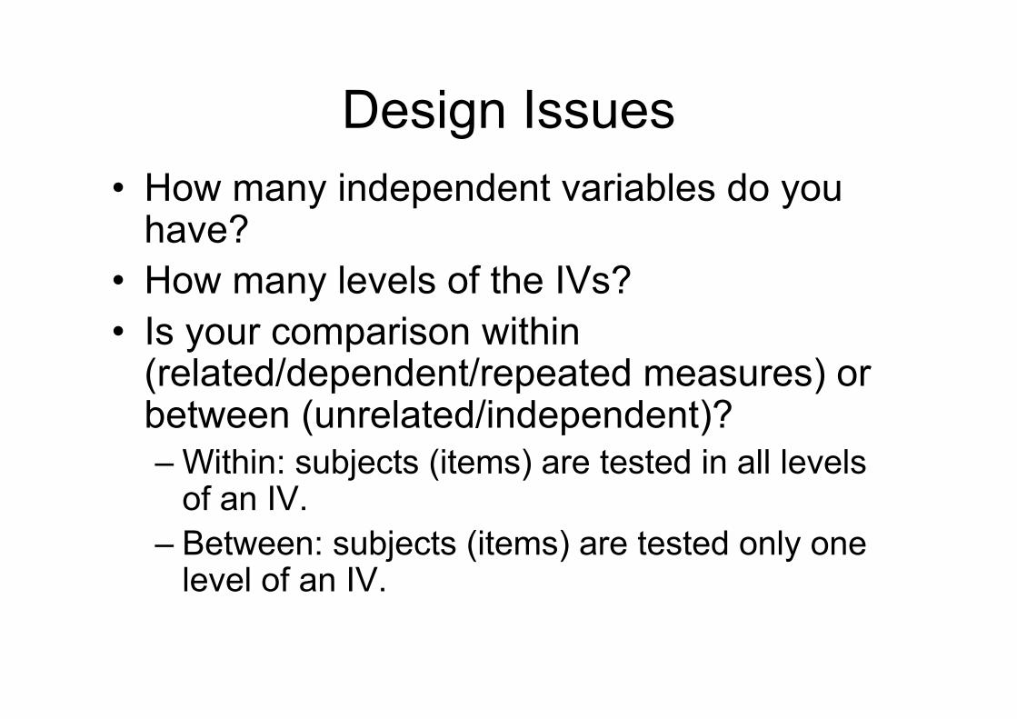
Design Issues• How many independent variables do you

have?• How many levels of the IVs?• Is your comparison within

(related/dependent/repeated measures) orbetween (unrelated/independent)?– Within: subjects (items) are tested in all levels

of an IV.– Between: subjects (items) are tested only one

level of an IV.

Types of Questions• Different questions are addressed with

different tests.– Are my two conditions different from one

another?– Is there a relationship between my two

factors?– Which combination of factors best explains

the patterns in my data?

What type of data do you have?

• Parametric tests make assumptions aboutyour data.– Normally distributed

– Independent **

– Homogeneity of variance

– At least interval scale **

• If your data violate these assumptions,consider using a non-parametric test.

Normality• Your data should be from

a normally distributedpopulation.– Normal distributions are

symmetrical ‘bell-shaped’distributions with the majorityof scores around the center.

– If you collect enough data, itshould be normallydistributed (Central LimitsTheorem)

• Evaluate normality by:– histogram– Kolmogorov-Smirnov test– Shapiro-Wilks’ test.

Data Assumptions

Homogeneity of Variance• The variance should not change systematically

throughout the data, especially not betweengroups of subjects or items.

• When you test different groups of subjects(monolinguals vs. bilinguals; test vs. control;trained vs. untrained), their variances should notdiffer.– If you test two corpora, the variance should not differ.

• Evaluate with– Levene’s test for between tests– Mauchly’s test of Sphericity in Repeated Measures

Data Assumptions

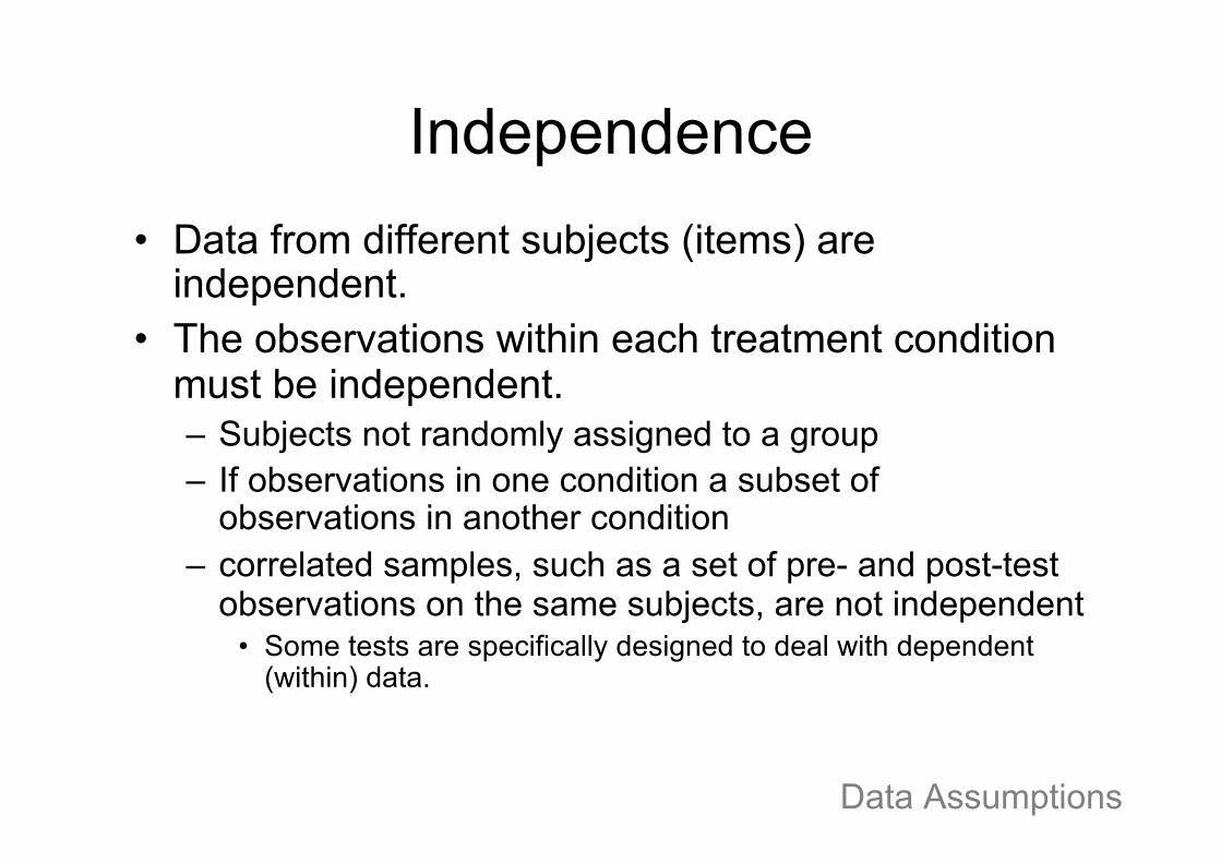
Independence• Data from different subjects (items) are

independent.• The observations within each treatment condition

must be independent.– Subjects not randomly assigned to a group– If observations in one condition a subset of

observations in another condition– correlated samples, such as a set of pre- and post-test

observations on the same subjects, are not independent• Some tests are specifically designed to deal with dependent

(within) data.

Data Assumptions

Types of Data• Nominal scale:

– Numbers represent qualitative features, not quantitative.– 1 not bigger than 2, just different; 1=masculine, 2 = feminine

• Ordinal Scale:– Rankings, 1 < 2 < 3 < 4, but differences between values not

important or constant; Likert scale data.• Interval Scale: like ordinal, but distances are equal

– Differences make sense, but ratios don’t (30°-20°=20°-10°, but 20°/10° is not twice as hot)

– e.g., temperature, dates• Ratio Scale: interval, plus a meaningful 0 point.

– Weight, length, reaction times, age

Data Assumptions

What type of data do you have?

• Parametric tests make assumptions aboutyour data.– Normally distributed

– Independent **

– Homogeneity of variance

– At least interval scale **

• Parametric tests are not robust to violationsof the starred assumptions

Data Assumptions

Jonckheeretrend

VarianceRatio (F)

Independent

Mann-Whitney

χ2

Independent Z-Independent t-VarianceRatio (F)

Independent

Spearman’srank correlationcoefficient

Page’sL trend

Wilcoxon

Sign

One-sampleproportions

VarianceRatio (F)

Related tOne-sample ZOnesample t

Product-momentcorrelationcoefficient(Pearson’s r)Linearregression

RelatedRelated

CorrelationK sampleTwo-SampleOne-Sample

Type of Research DesignTy

pe o

f Dat

a

Para

met

ricN

on-p

aram

etric

Miller, 1984

Picking a test

Between-subjects analyses

χ2Kruskal-Wallis

Between-subjectsANOVA

Three ormore

χ2Mann-Whitney

Independentsamples t-test

two

Nonparametric -nominal

Nonparametric - ordinal

Parametricscores

# ofconditions

Picking a test

Within-subjects analyses

noneFriedmanRepeatedMeasuresANOVA

Three ormore

noneWilcoxonDependentsamples t

two

Nonparametric -nominal

Nonparametric - ordinal

Parametricscores

# ofconditions

Picking a test

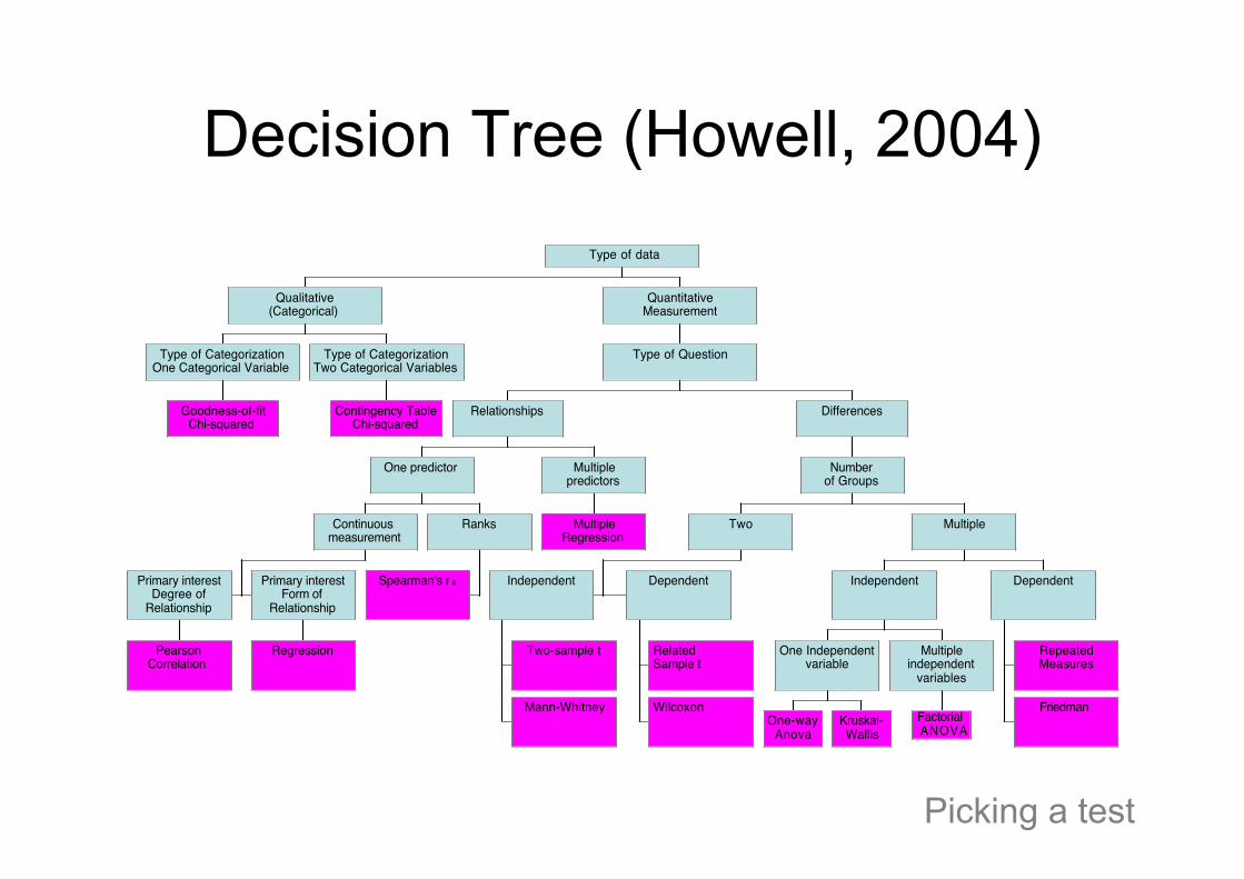
Decision Tree (Howell, 2004)

Goodness-of-fitChi-squared

Type of CategorizationOne Categorical Variable

Contingency TableChi-squared

Type of CategorizationTwo Categorical Variables

Qualitative(Categorical)

PearsonCorrelation

Primary interestDegree of

Relationship

Regression

Primary interestForm of

Relationship

Continuousmeasurement

Spearman's r s

Ranks

One predictor

MultipleRegression

Multiplepredictors

Relationships

Two-sample t

Mann-Whitney

Independent

RelatedSample t

Wilcoxon

Dependent

Two

One-wayAnova

Kruskal-Wallis

One Independentvariable

FactorialANOVA

Multipleindependent

variables

Independent

RepeatedMeasures

Friedman

Dependent

Multiple

Numberof Groups

Differences

Type of Question

QuantitativeMeasurement

Type of data

Picking a test

How do stats work and whydo we use them?

• We observe some behavior, of individuals,the economy, our computer models, etc.

• We want to say something about thisbehavior. We’d like to say something thatextends beyond just the observations wemade to future behaviors, past behaviors,unobserved behaviors.

Types of Statistical Analyses

• Descriptive statistics: summarizing anddescribing the important characteristics ofthe data.

• Inferential statistics: decide if a pattern,difference or relations found with a sampleis representative and true of the population.

Why go beyond descriptives?

170190

Brides’ mean heightMonks’ mean height

• The mean might make it look like monks are taller, butmaybe that that doesn’t represent the truth.

Q: Are monks taller than brides?

Is this difference REAL?• Descriptive difference

– Milk costs .69 at Plus and .89 at Mini-mall• Is this a real difference?

• Subjective difference• Is the difference important enough to me? Is it worth my while

to travel farther to pay less?

• Statistical difference– Is Plus generally cheaper than Mini-mall?

• How representative of the prices is milk?– Are all Plus stores cheaper than all Mini-malls?

• How representative of all Plus stores is my Plus?

• Inferential statistics help us answer these questionswithout the need for an exhaustive survey.

How to inferential statisticswork?

• Different statistical methods attempt to builda model of the data using hypothesizedfactors to account for the characteristics ofthe observed pattern.

• One simple model of the data is the MEAN

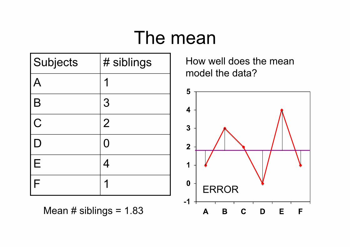
ERROR

The mean

1F

4E

0D

2C

3B

1A

# siblingsSubjects

Mean # siblings = 1.83

How well does the meanmodel the data?

Variance• Variance is an index of error between the

mean and the individual observations.

!

xi" x( )#

!

xi" x( )#

2

• Sum of error is offset by positive and negative numbers– Take the square of each error value

• Sum of squared errors (SS) will increase the more data you collect.– Large number ≠ bad estimate of # of siblings

• Divide the sum of squared errors by N-1• Variance (s2) = SS/N-1

Standard Deviation

• Variance gives us measure in unitssquared, so not comparable to directly tothe units measured.– If your data has a range from 1-100, you could

easily have a variance of > 100, which is notthat informative an index of error.

• Standard Deviation is a measure of howwell the mean represents the data.

!

s = SSN "1

Sampling• Sampling is a random selection of representative

members of a population.• If you had access to all members of a population then

you would not need to conduct inferential statistics tosee whether some observation generalizes to thewhole population.

• Normally, we only have access to a (representative)subset.

• Most random samples tend to be fairly typical of thepopulation, but there is always variation.

Standard Error• Variance and Standard Deviation index the

relationship between the mean of observationsand individual observations.– Comment on the SAMPLE

• Standard error is similar to SD but it applies tothe relationship between a sample mean and thepopulation.

• Standard errors give you a measure of howrepresentative your sample is of the population.– A large standard error means your sample is not very

representative of the population. Small SE means it isrepresentative.

!

MSE = S / N

Normality and SD

• The combination of measures of varianceand assumptions of normality underliehypothesis testing and inferential statistics.

• Statistical tests output a probability that anobserved pattern (difference or relationship)are true of the population.

• How does this work?

Normal Curves• Normal curves can be defined by their

mean and variance.• Z-distribution has mean = 0 & SD = 1• x: N (0,1)

95% of data points are within about 2 SD of mean

Normal Curves

• Given these characteristics of normalcurves, you can calculate what percentageof the data points are above or below someany value.

• This is a basic principle behind most of thecommon inferential tests.

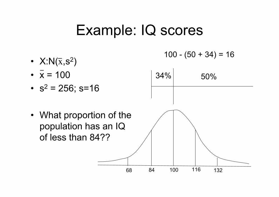
Example: IQ scores

• X:N(x,s2)• x = 100• s2 = 256; s=16

• What proportion of thepopulation has an IQof less than 84??

10084 11668 132

50%34%

100 - (50 + 34) = 16

Standard normal transformation• You can calculate the proportion above or below

or between any (2) point(2) for any normal curve.

• First, calculate how many SD a value is frommean. Then look up value in table.

10084 11668 132

!

z(x) =x " x

"

s

!

z(108) =108 "100

16= 0.5

http://davidmlane.com/hyperstat/z_table.htmlhttp://www.statsoft.com/textbook/sttable.html#z

Normal curves as gateway toinferential statistic

• Given the distribution of normal curves, you can now identify thelikelihood that two means come from the same population.

• Imagine you want to know if jetlag results in poor test taking ability.You test some kids who just flew from Edinburgh to Chicago.

• You know the population mean is 100 with SD=16. The sample youdraw has a mean test result of 84.– What can we conclude?

• We know that 16% of the general population has an IQ of 84 or below,so you want to know the chances of drawing, at random, a samplewith mean IQ of 84.

• If the chances are p > .05 (or whatever cut off you want to use) you’dconclude that jetlag doesn’t have a reliable effect on IQ. If p < .05 youwould conclude that it does.– That is statistical significance!!!

Sources of Variability

• There are two sources of variability in your data.– Variability caused by subjects and items (individual

differences)– Variability induced by your manipulation

• To find a statistically significant effect, you wantthe variation between conditions to be greaterthan within conditions.

• Note: if you don’t have variance in your data (e.g.,cuz the program is deterministic and alwaysbehaves the same way) inferential stats might notbe for you.

Variability of results

High variability(between 2 conditions)

median

Medium variability

Low variability (differencebetween conditions is reliable andcan be generalized)

Tests for finding differences

Hour 2.2

Comparing two means

• If you are interested in knowing whetheryour two conditions differ from one anotherAND you have only 2 conditions.

• Evaluates the influence of yourIndependent Variable on your DependentVariable.

Test options: 2 conditions

• Parametric data: the popular t-test– 1 sample– Independent pairs– related pairs

• Non-parametric equivalents– Related pairs– Independent pairs

1-sample t-test• Compares mean of sample data to theoretical population

mean.• Standard error used to gauge the variability between

sample and population means.– The difference between the sample mean and the hypothesized

population mean must be greater than the normal variance foundwithin the population to conclude that you have a significant effectof the IV.

– Standard error small, samples should have similar means; SElarge, large diffs in means by chance are possible.

!

t =X "µ

standarderror ofmeanµ=estimated pop mean

Parametric tests of differences

How big is your t?

• How large should the t-statistic be?• The probability of a difference reflecting a REAL

effect is determined by the characteristics of theparticular curve.– Z and t curves are normal curves.– F and χ2 are positively skewed curves.– P-values are sensitive to the size of the sample, so a t

of 2.5 might be significant for a large N but not for asmall N.

– Tables or statistical programs relate t-values, degreesof Freedom and test statistics.

– http://faculty.vassar.edu/lowry/tabs.html#t

Independent samples t-test

• Compares means of two independentgroups (between-design).

• Same underlying principle (signal-to-noise)based on standard errors.

• Bigger t-value --> larger effects

!

t =(X "Y ) " (µ

1"µ

2)

Estimateof SE of difference

between twosamplemeans

Parametric tests of differences

Related t-test

• Compares the means of two relatedgroups; either matched-pairs within-subjects designs.– Test the same person in both conditions.– Reduce the amount of unsystematic variation

introduced into the experiment.

Parametric tests of differences

Non-parametric tests

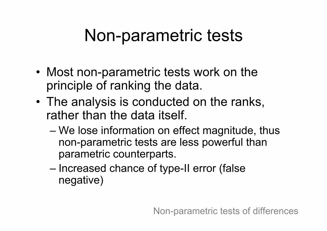
• Most non-parametric tests work on theprinciple of ranking the data.

• The analysis is conducted on the ranks,rather than the data itself.– We lose information on effect magnitude, thus

non-parametric tests are less powerful thanparametric counterparts.

– Increased chance of type-II error (falsenegative)

Non-parametric tests of differences

814613Sub4a/b

715410Sub3a/b

51128Sub2a/b

3916Sub1a/b

RankCond 2RankCond 1

Ranking the Responses

Non-parametric tests of differences

Non-parametric tests

• Mann-Whitney: 2 independent pairs test.– Operates on ranking the responses,

independent of condition membership.– Equal sample size not required.

• Wilcoxon sign ranked: 2 related pairs– rank the absolute value of differences from a

pair– Equal sample size required

Non-parametric tests of differences

Sign Test• Alternative to either the 2 related or 2

independent (with random pairing) non-parametric tests.

• Requires equal sample size.• Simply counts number of positive vs.

negative differences betweenconditions.

• If no difference, 50/50 split expected.• Calculate the P (n +)

Non-parametric tests of differences

Comparing more thantwo means

Hour 2.85

ANOVA

• Analysis of Variance– Similar to t-test in that it also calculates a

Signal-to-noise ratio, F.• Signal = variance between conditions• Noise = variance within conditions

– Can analyze more than 2 levels of a factor.• Not appropriate to simply conduct multiple t-tests

because of inflation of p-value.– Can analyze more than 1 factor.– Can reveal interactions between factors.

Parametric tests for more than 2 conditions

1-way ANOVA• Analogue to independent groups t-test for 3 or more levels

of one factor.– A 1-way anova with 2 levels is equivalent to a t-test. P-values the

same: F=t2

143966748,512

Total

6081,776141857530,417

WithinGroups

,0008,97954609,048

2109218,095

BetweenGroups

Sig.FMeanSquare

dfSum ofSquares

Parametric tests for more than 2 conditions

ANCOVA• Analysis of Covariance

– If you have continuous variable that was notmanipulated but that might add variance,• like word frequency, subject age, years of

programming experience, sentence length, etc…– you can factor out the variance attributed to this

covariate.– This removes the error variance and makes a

large ratio more likely.– Available for independent and repeated

measures variantsParametric tests for more than 2 conditions

Factorial univariate ANOVA

• When you have more than one IV but theanalysis remains between subjects.

• This analysis allows you to test the ‘maineffect’ of each independent variable andalso the interaction between the variables.

• If you have multiple dependent variables,you can use multivariate anova.

Parametric tests for more than 2 conditions

Repeated Measures Anova

• Within subjects

• This analysis is appropriate for data fromjust 1 IV, multiple IVs, for mixed designsand can factor out covariates.

Parametric tests for more than 2 conditions

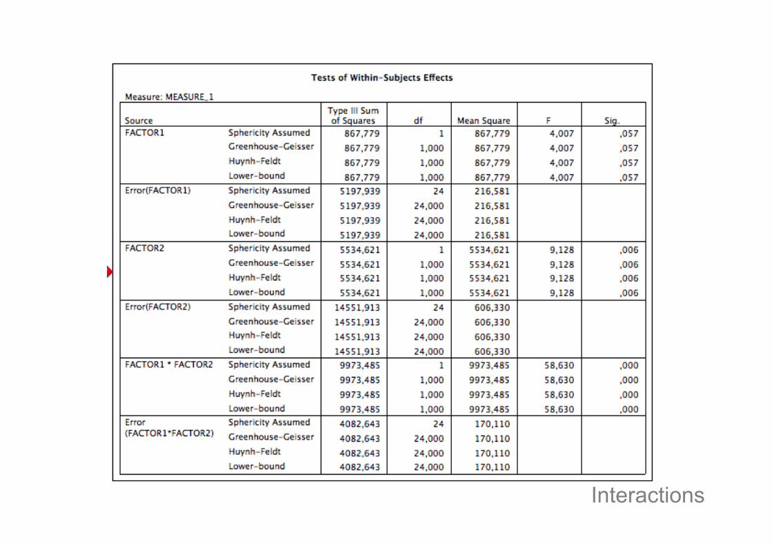
Main effects and interactions• Let‘s assume we have 2 factors with 2 levels

each that we manipulated in an experiment:

– Factor one: lexical frequency of words (high frequencyand low frequency)

– Factor two: word length (long words and short words)

• We measured reaction times for a naming task.

• In a repeated measures ANOVA we canpotentially find 2 main effects and 1 interaction

Interactions

• Main effect of word length (long words 350 ms, short words 250 ms)• No main effect of frequency (high frequency 300 ms, low frequency 300 ms)• Interaction between word length and frequency (i.e., frequency has a different influence

on long words and short words)

Main effects and interactions

200

400

300 300

0

50

100

150

200

250

300

350

400

450

short words long words

high frequency

low frequency

Interactions

Interactions

Interactions

• Interactions indicate that independentvariable X influences the dependentvariable differently depending on the levelof independent variable Y.

– Interpret your main effects with theconsideration of the interaction.

– You can have an interaction with no maineffects.

Interactions

Types of interactions

• Antagonistic interaction: the twoindependent variables reverse each other’seffects.

• Synergistic interaction: a higher level of Benhances the effect of A.

• Ceiling-effect interaction: the higher level ofB reduces the differential effect of A.

Interactions

Antagonistic Interaction

0

1

2

3

4

5

6

7

A1 A2

B1

B2

main

Effect

of A

Interactions

• the two independentvariables reverseeach other’s effects.

Interactions

Synergistic Interaction

0

2

4

6

8

10

12

14

A1 A2

B1

B2

main

Effect

of A

• a higher level of Benhances the effect ofA.

Ceiling-effect Interaction

0

2

4

6

8

10

12

14

A1 A2

B1

B2

main

Effect

of A

Interactions

• The higher level of Breduces thedifferential effect of A.

Interpreting Interactions

• If you want to say that two factorsinfluence each other, you need todemonstrate an interaction

• If you want to say that a factor affects twoDVs differently, you need to demonstratean interaction.

Interactions

Non-parametric alternatives

• If you have 1 independent variable withmore than 2 levels (K levels):

• Kruskal Wallis independent test forbetween designs

• Friedman related samples test for withindesigns.

Non-parametric tests of more than 2 conditions

Pearson’s Chi-squared• Appropriate if:

– 1 Categorical Dependent Variable (dichotomous data)– 2 Independent variables with at least 2 levels

• Detects whether there is a significant associationbetween two variables (no causality)

• Assumptions:– Each person or case contributes to only one cell of the

contingency table.• Not appropriate for repeated measures.

– takes raw data, not proportions.– Values in all cells should be > 5 (else do fisher’s exact

test)

Non-parametric tests of more than 2 conditions

Hierarchical Loglinear Analysis

• If you have more than 3 IndependentVariables and are interested in the HigherOrder Interactions.

• Designed to analyze multi-way contingencytables

• Table entries are frequencies– Functionally similar to χ2

Non-parametric tests of more than 2 conditions

Summary for anovas• If you have 1 independent factor with K

levels between subjects: 1-way ANOVA• If you have a covarying factor and one or

more between subjects independentfactors, use univariate ANOVA

• If you have repeated measures design,with 1 or more manipulated factors, with orwithout a covariate or an additionalbetween subjects factor, use RepeatedMeasures

Correlations &Linear Regressions

Hour 3.25

Question

• Are two conditions different?

• What relationship exists between two ormore variables?– Positively related: as x goes, so goes y.– Negatively related: whatever x does, y does the

opposite.– No relationship.

Correlations

Example of linear correlation

Record Sales (thousands)

4003002001000

Advert

sin

g B

ud

get

(thousand

s o

f pounds)

3000

2000

1000

0

-1000

Correlations

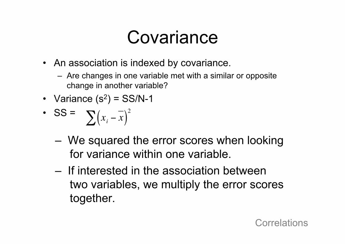
Covariance• An association is indexed by covariance.

– Are changes in one variable met with a similar or oppositechange in another variable?

• Variance (s2) = SS/N-1• SS =

!

xi" x( )#

2

– We squared the error scores when lookingfor variance within one variable.

– If interested in the association between two variables, we multiply the error scorestogether.

Correlations

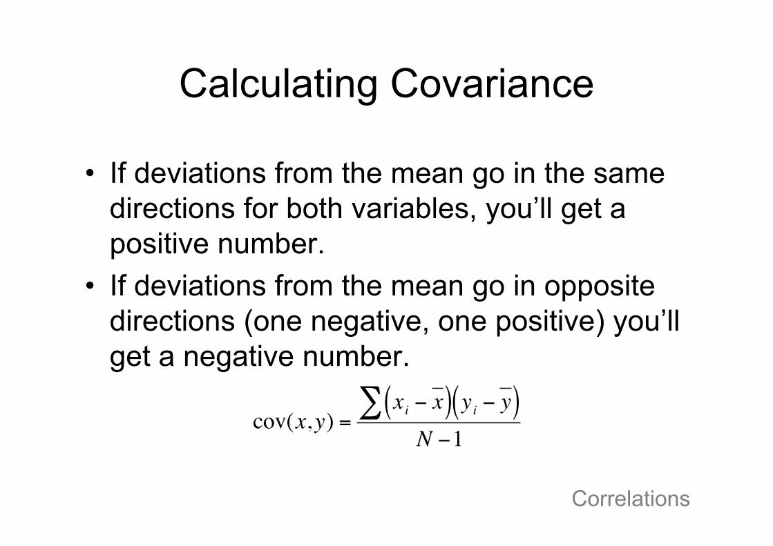
Calculating Covariance

• If deviations from the mean go in the samedirections for both variables, you’ll get apositive number.

• If deviations from the mean go in oppositedirections (one negative, one positive) you’llget a negative number.

!

cov(x,y) =xi " x( ) yi " y( )#N "1

Correlations

Interpreting linear relations

• Correlation coefficient [r] = linear relationship between twovariables. Measures the amount of spread around animaginary line through the center.

• r2 = proportion of common variation in the two variables(strength or magnitude of the relationship). Proportion ofthe variance in 1 set of score that can be accounted for byknowing X.

• Outliers? A single outlier can greatly influence the strengthof a correlation.

Correlations

Effect of outliers

One approach to dealing with outliers is to see if they arenon-representative (i.e., at the far end of the normal distribution).If so, they should be removed.

Correlations

Types of correlations

• Bivariate correlation: between two variable– Pearson’s correlation coefficient for parametric data

(interval or ratio data)

• Partial correlation: relationship between twovariables while ‘controlling’ the effect of one ormore additional variables.

• Biserial correlation: when one variable isdichotomous (e.g., alive vs. dead, male vs. female)

Correlations

Drawing conclusions• Correlations only inform us about a

relationship between two or morevariables.

• Not able to talk about directionality orcausality.– An increase in X does not CAUSE an

increase in Y or vise versa. Cause could befrom unmeasured third variable.

Correlations

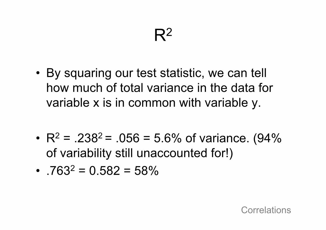
R2

• By squaring our test statistic, we can tellhow much of total variance in the data forvariable x is in common with variable y.

• R2 = .2382 = .056 = 5.6% of variance. (94%of variability still unaccounted for!)

• .7632 = 0.582 = 58%

Correlations

Non-parametric correlations

• Spearman’s Rho– For non-interval data– Ranks the data and then applies Pearson’s

equation to ranks.• Kendall’s Tau

– Preferred for small data sets with many tiedrankings.

Correlations

Simple Linear Regressions

Hour 2.75

Regressions• Correlations detect associations between

two variables.– Say nothing of causal relationships or

directionality– Can’t predict behavior on one variable given a

value behavior for another variable

• With Regression models we can predictvariable Y based on variable X.

Regressions

Simple Linear Regressions

• A line is fit to the data (similar to thecorrelations line).– Best line is one that produces the smallest sum

of squares from regression line to data points.

• Evaluation based on improvement ofprediction relative to using the mean.

Regressions

Hypothetical Data

0

10

20

30

40

50

60

70

80

0 5 10 15 20 25

outcome variable

Pred

icto

r v

aria

ble

MeanRegressions

Error from Mean

0

10

20

30

40

50

60

70

80

0 5 10 15 20 25

outcome variable

Pre

dic

tor v

aria

ble

MeanRegressions

Error from regression line

0

10

20

30

40

50

60

70

80

0 5 10 15 20 25

outcome variable

Pred

icto

r v

aria

ble

Mean

Regressionline

Regressions

Regression Results

• The best regression line has the lowestsum of squared errors

• Evaluation of the regression model isachieved via– R2 = tells you % of variance accounted for by

the regression line (as with correlations)– F = Evaluates improvement of regression line

compared to the mean as a model of the data.

Regressions

Predicting New Values

• Equation for line:– Y - output value– X = predictor value– β0 = intercept (constant. Value of Y without

predictors)– β1 = slope of line (value for predictor)– ε = residual (error)!

Y = "0

+ "1Xi+ #

i

Regressions

Multiple Regression

• Extends principles of simple linearregression to situation with multiplepredictor variables.

• We seek to find the linear combination ofpredictors that correlate maximally with theoutcome variable.

!

Y = "0

+ "1Xi+ "

nXn

+ #i

Predictor 1 Predictor 2 Regressions

Multiple Regression, con’t

• R2 gives the % variance accounted for bythe model consisting of the multiplepredictors.

• T-test tell you independent contribution ofeach predictor in capturing data.

• Logistic Regressions are appropriate fordichotomous data!

Regressions

R2 & Adjusted R2 should be similar

Adjusted R2 = variance in Pop

Is the model an improvementover the mean or over a priormodel?

β = Change inoutcome resulting inchange in predictor

Tests that lineisn’t horizontal

Regressions

Improvement over meanImprovement over 1stblock

Units expressed as standarddeviation for better comparison

T-test givesimpression of whethernew predictorsimprove model

Degree each predictoreffects outcome ifeffects of otherpredictors held constant

Summary• You should know which of the common tests are

applicable to what types of data, designs andquestions.

• You should also have enough backgroundknowledge to help you understand what you readon-line or in statistics books.

• You should have an idea which tests might beuseful for the type of data you have.

Informative Websites• http://faculty.vassar.edu/lowry/VassarStats.html

• http://www.uwsp.edu/psych/stat/

• http://www.richland.edu/james/lecture/m170/

• http://calcnet.mth.cmich.edu/org/spss/index.htm for spssvideos!

• http://espse.ed.psu.edu/edpsych/faculty/rhale/statistics/Investigating.htm

• Or, just google the test you are interested in.