Introduction to Fluids in Motionabuhasan/content/teaching/skmm2313/... · Present several examples...
39
87 3 Introduction to Fluids in Motion Outline 3.1 Introduction 3.2 Description of Fluid Motion 3.2.1 Lagrangian and Eulerian Descriptions of Motion 3.2.2 Pathlines, Streaklines, and Streamlines 3.2.3 Acceleration 3.2.4 Angular Velocity and Vorticity 3.3 Classification of Fluid Flows 3.3.1 One-,Two-, and Three-Dimensional Flows 3.3.2 Viscous and Inviscid Flows 3.3.3 Laminar and Turbulent Flows 3.3.4 Incompressible and Compressible Flows 3.4 The Bernoulli Equation 3.5 Summary Chapter Objectives The objectives of this chapter are to: ▲ Mathematically describe the motion of a fluid. ▲ Express the acceleration and vorticity of a fluid particle given the velocity components. ▲ Describe the deformation of a fluid particle. ▲ Classify various fluid flows. Is a flow viscous, is it turbulent, is it incompres- sible, is it a uniform flow? ▲ Derive the Bernoulli equation and identify its restrictions. ▲ Present several examples and numerous problems that demonstrate how fluid flows are described, how flows are classified, and how Bernoulli’s equa- tion is used to estimate flow variables. Copyright 2010 Cengage Learning. All Rights Reserved. May not be copied, scanned, or duplicated, in whole or in part. Due to electronic rights, some third party content may be suppressed from the eBook and/or eChapter(s). Editorial review has deemed that any suppressed content does not materially affect the overall learning experience. Cengage Learning reserves the right to remove additional content at any time if subsequent rights restrictions require it.
Transcript of Introduction to Fluids in Motionabuhasan/content/teaching/skmm2313/... · Present several examples...

87
3Introduction to Fluids in Motion
Outline3.1 Introduction3.2 Description of Fluid Motion
3.2.1 Lagrangian and Eulerian Descriptions of Motion3.2.2 Pathlines, Streaklines, and Streamlines3.2.3 Acceleration3.2.4 Angular Velocity and Vorticity
3.3 Classification of Fluid Flows3.3.1 One-, Two-, and Three-Dimensional Flows3.3.2 Viscous and Inviscid Flows3.3.3 Laminar and Turbulent Flows3.3.4 Incompressible and Compressible Flows
3.4 The Bernoulli Equation3.5 Summary
Chapter ObjectivesThe objectives of this chapter are to:
▲ Mathematically describe the motion of a fluid.▲ Express the acceleration and vorticity of a fluid particle given the velocity
components.▲ Describe the deformation of a fluid particle.▲ Classify various fluid flows. Is a flow viscous, is it turbulent, is it incompres-
sible, is it a uniform flow?▲ Derive the Bernoulli equation and identify its restrictions.▲ Present several examples and numerous problems that demonstrate how
fluid flows are described, how flows are classified, and how Bernoulli’s equa-tion is used to estimate flow variables.
Copyright 2010 Cengage Learning. All Rights Reserved. May not be copied, scanned, or duplicated, in whole or in part. Due to electronic rights, some third party content may be suppressed from the eBook and/or eChapter(s). Editorial review has deemed that any suppressed content does not materially affect the overall learning experience. Cengage Learning reserves the right to remove additional content at any time if subsequent rights restrictions require it.

3.1 INTRODUCTION
This chapter serves as an introduction to all the following chapters that deal withfluid motions. Fluid motions manifest themselves in many different ways. Somecan be described very easily, while others require a thorough understanding ofphysical laws. In engineering applications, it is important to describe the fluidmotions as simply as can be justified. This usually depends on the required accu-racy. Often, accuracies of � 10% are acceptable, although in some applicationshigher accuracies have to be achieved. The general equations of motion are verydifficult to solve; consequently, it is the engineer’s responsibility to know whichsimplifying assumptions can be made. This, of course, requires experience and,more importantly, an understanding of the physics involved.
Some common assumptions used to simplify a flow situation are related tofluid properties. For example, under certain conditions, the viscosity can affectthe flow significantly; in others, viscous effects can be neglected, greatly simplify-ing the equations without significantly altering the predictions. It is well knownthat the compressibility of a gas in motion should be taken into account if thevelocities are very high. But compressibility effects do not have to be taken intoaccount to predict wind forces on buildings or to predict any other physical quan-tity that is a direct effect of wind. Wind speeds are simply not high enough.Numerous examples could be cited. After our study of fluid motions, the appro-priate assumptions used should become more obvious.
This chapter has three sections. In the first section we introduce the readerto some important general approaches used to analyze fluid mechanics problems.In the second section we give a brief overview of different types of flow, such ascompressible and incompressible flows, and viscous and inviscid flows. Detaileddiscussions of each of these flow types follow in later chapters. The third sectionintroduces the reader to the commonly used Bernoulli equation, an equation thatestablishes how pressures and velocities vary in a flow field. The use of this equa-tion, however, requires many simplifying assumptions, and its application is,therefore, limited.
3.2 DESCRIPTION OF FLUID MOTION
The analysis of complex fluid flow problems is often aided by the visualization offlow patterns, which permit the development of a better intuitive understandingand help in formulating the mathematical problem. The flow in a washingmachine is a good example. An easier, yet difficult problem is the flow in thevicinity of where a wing attaches to a fuselage, or where a bridge support inter-acts with the water at the bottom of a river. In Section 3.2.1 we discuss thedescription of physical quantities as a function of space and time coordinates.Thesecond topic in this section introduces the different flow lines that are useful inour objective of describing a fluid flow. Finally, the mathematical description ofmotion is presented.
3.2.1 Lagrangian and Eulerian Descriptions of Motion
In the description of a flow field, it is convenient to think of individual particleseach of which is considered to be a small mass of fluid, consisting of a large number
88 Chapter 3 / Introduction to Fluids in Motion
KEY CONCEPT Undercertain conditions, viscouseffects can be neglected.
Copyright 2010 Cengage Learning. All Rights Reserved. May not be copied, scanned, or duplicated, in whole or in part. Due to electronic rights, some third party content may be suppressed from the eBook and/or eChapter(s). Editorial review has deemed that any suppressed content does not materially affect the overall learning experience. Cengage Learning reserves the right to remove additional content at any time if subsequent rights restrictions require it.

Sec. 3.2 / Description of Fluid Motion 89
of molecules, that occupies a small volume �V that moves with the flow. If the fluidis incompressible, the volume does not change in magnitude but may deform. If thefluid is compressible, as the volume deforms, it also changes its magnitude. In bothcases the particles are considered to move through a flow field as an entity.
In the study of particle mechanics, where attention is focused on individualparticles, motion is observed as a function of time. The position, velocity, andacceleration of each particle are listed as s(x0, y0, z0, t), V(x0, y0, z0, t), and a(x0, y0, z0, t), and quantities of interest can be calculated. The point (x0, y0, z0)locates the starting point—the name—of each particle. This is the Lagrangiandescription, named after Joseph L. Lagrange (1736–1813), of motion that is used ina course on dynamics. In the Lagrangian description many particles can be fol-lowed and their influence on one another noted.This becomes, however, a difficulttask as the number of particles becomes extremely large in even the simplest fluidflow.
An alternative to following each fluid particle separately is to identify pointsin space and then observe the velocity of particles passing each point; we canobserve the rate of change of velocity as the particles pass each point, that is,�V/�x, �V/�y, and �V/�z, and we can observe if the velocity is changing with timeat each particular point, that is, �V/�t. In this Eulerian description, named afterLeonhard Euler (1707–1783), of motion, the flow properties, such as velocity, arefunctions of both space and time. In Cartesian coordinates the velocity isexpressed as V � V(x, y, z, t). The region of flow that is being considered is calleda flow field.
An example may clarify these two ways of describing motion. An engineer-ing firm is hired to make recommendations that would improve the traffic flowin a large city. The engineering firm has two alternatives: Hire college studentsto travel in automobiles throughout the city recording the appropriate observa-tions (the Lagrangian approach), or hire college students to stand at the inter-sections and record the required information (the Eulerian approach).A correctinterpretation of each set of data would lead to the same set of recommenda-tions, that is, the same solution. In this example it may not be obvious whichapproach would be preferred; in an introductory course in fluids, however, theEulerian description is used exclusively since the physical laws using theEulerian description are easier to apply to actual situations. Yet, there are exam-ples where a Lagrangian description is needed, such as drifting buoys used tostudy ocean currents.
If the quantities of interest do not depend on time, that is, V � V(x, y, z), theflow is said to be a steady flow. Most of the flows of interest in this introductorytextbook are steady flows. For a steady flow, all flow quantities at a particularpoint are independent of time, that is,
��
�
Vt� � 0 �
�
�
p
t� � 0 �
�
�
r
t� � 0 (3.2.1)
to list a few. It is implied that x, y, and z are held fixed in the above. Note that theproperties of a fluid particle do, in general, vary with time; the velocity and pres-sure vary with time as a particular fluid particle progresses along its path in aflow, even in a steady flow. In a steady flow, however, properties do not vary withtime at a fixed point.
Lagrangian: Description ofmotion where individualparticles are observed as afunction of time.
Steady flow: Where flowquantities do not depend ontime.
Eulerian: Description ofmotion where the flowproperties are functions ofboth space and time.
Flow field: The region ofinterest in a flow.
Eulerian vs. Lagrangian,31–33
Copyright 2010 Cengage Learning. All Rights Reserved. May not be copied, scanned, or duplicated, in whole or in part. Due to electronic rights, some third party content may be suppressed from the eBook and/or eChapter(s). Editorial review has deemed that any suppressed content does not materially affect the overall learning experience. Cengage Learning reserves the right to remove additional content at any time if subsequent rights restrictions require it.

3.2.2 Pathlines, Streaklines, and Streamlines
Three different lines help us in describing a flow field. A pathline is the locusof points traversed by a given particle as it travels in a field of flow; the path-line provides us with a “history” of the particle’s locations. A photograph of apathline would require a time exposure of an illuminated particle. A photo-graph showing pathlines of particles below a water surface with waves is givenin Fig. 3.1.
A streakline is defined as an instantaneous line whose points are occupied byall particles originating from some specified point in the flow field. Streaklinestell us where the particles are “right now.”A photograph of a streakline would bea snapshot of the set of illuminated particles that passed a certain point.Figure 3.2 shows streaklines produced by the continuous release of a small-diameter stream of smoke as it moves around a cylinder.
Pathline: The history of aparticle’s locations.
90 Chapter 3 / Introduction to Fluids in Motion
Streakline: An instantaneousline.
Fig. 3.1 Pathlines underneath a wave in a tank of water.(Photograph by A. Wallet and F. Ruellan. Courtesy of M. C. Vasseur.)
Fig. 3.2 Streaklines in the unsteady flow around a cylinder.(Photography by Sadatoshi Taneda. From Album of Fluid Motion, 1982,The Parabolic Press, Stanford, California.)
Pathlines, 91
Streaklines, 122
Streamlines, 122
Copyright 2010 Cengage Learning. All Rights Reserved. May not be copied, scanned, or duplicated, in whole or in part. Due to electronic rights, some third party content may be suppressed from the eBook and/or eChapter(s). Editorial review has deemed that any suppressed content does not materially affect the overall learning experience. Cengage Learning reserves the right to remove additional content at any time if subsequent rights restrictions require it.

Sec. 3.2 / Description of Fluid Motion 91
A streamline is a line in the flow possessing the following property: the veloc-ity vector of each particle occupying a point on the streamline is tangent to thestreamline. This is shown graphically in Fig. 3.3. An equation that expresses thatthe velocity vector is tangent to a streamline is
(3.2.2)
since V and dr are in the same direction, as shown in the figure; recall that thecross product of two vectors in the same direction is zero. This equation will beused in future chapters as the mathematical expression of a streamline. A pho-tograph of a streamline cannot be made directly. For a general unsteady flowthe streamlines can be inferred from photographs of short pathlines of a largenumber of particles.
A streamtube is a tube whose walls are streamlines. Since the velocity is tan-gent to a streamline, no fluid can cross the walls of a streamtube. The streamtubeis of particular interest in fluid mechanics. A pipe is a streamtube since its wallsare streamlines; an open channel is a streamtube since no fluid crosses the wallsof the channel. We often sketch a streamtube with a small cross section in theinterior of a flow for demonstration purposes.
In a steady flow, pathlines, streaklines, and streamlines are all coincident. Allparticles passing a given point will continue to trace out the same path since thevelocity in our Eulerian system does not change with time; hence the pathlinesand streaklines coincide. In addition, the velocity vector of a particle at a givenpoint will be tangent to the line that the particle is moving along; thus the line isalso a streamline. Since the flows that we observe in laboratories are invariablysteady flows, we call the lines that we observe streamlines even though they mayactually be streaklines, or for the case of time exposures, pathlines.
3.2.3 Acceleration
The acceleration of a fluid particle is found by considering a particular particleshown in Fig. 3.4. Its velocity changes from V(t) at time t to V(t � dt) at timet � dt. The acceleration is, by definition,
V � dr � 0
Streamline: The velocityvector is tangent to thestreamline.
Streamtube: A tube whosewalls are streamlines.
x
V
V
VV
z
y
dr
r
Fig. 3.3 Streamline in a flow field.
KEY CONCEPT In asteady flow, pathlines,streaklines, and streamlinesare all coincident.
Copyright 2010 Cengage Learning. All Rights Reserved. May not be copied, scanned, or duplicated, in whole or in part. Due to electronic rights, some third party content may be suppressed from the eBook and/or eChapter(s). Editorial review has deemed that any suppressed content does not materially affect the overall learning experience. Cengage Learning reserves the right to remove additional content at any time if subsequent rights restrictions require it.

(3.2.3)
where dV is shown in Fig. 3.4. The velocity vector V is given in component form as
V � u ı � v j � „ k (3.2.4)
where (u, v, „) are the velocity components in the x-, y-, and z- directions, respec-tively, and ı, j and k are the unit vectors. The quantity dV is, using the chain rulefrom calculus with V � V(x, y, z, t),
dV � ��
�
Vx� dx � �
�
�
Vy� dy � �
�
�
Vz� dz � �
�
�
Vt� dt (3.2.5)
This gives the acceleration using Eg. 3.2.3 as
a � ��
�
Vx� �
ddxt� � �
�
�
Vy� �
ddyt� � �
�
�
Vz� �
ddzt� � �
�
�
Vt� (3.2.6)
Since we have followed a particular particle, as in Fig. 3.4, we recognize that
�ddxt� � u �
ddyt� � v �
ddzt� � „ (3.2.7)
The acceleration is then expressed as
(3.2.8)
The scalar component equations of the above vector equation for Cartesian coor-dinates are written as
a � u ��
�
Vx� � v �
�
�
Vy� � „ �
�
�
Vz� � �
�
�
Vt�
a � �ddVt�
92 Chapter 3 / Introduction to Fluids in Motion
Fluid particleat time t
V(t)
V(t) V(t + dt)
V(t + dt)
x
z
y
dV
The same fluid particleat time t + dt
Fig. 3.4 Velocity of a fluid particle.
Copyright 2010 Cengage Learning. All Rights Reserved. May not be copied, scanned, or duplicated, in whole or in part. Due to electronic rights, some third party content may be suppressed from the eBook and/or eChapter(s). Editorial review has deemed that any suppressed content does not materially affect the overall learning experience. Cengage Learning reserves the right to remove additional content at any time if subsequent rights restrictions require it.
Sec. 3.2 / Description of Fluid Motion 93
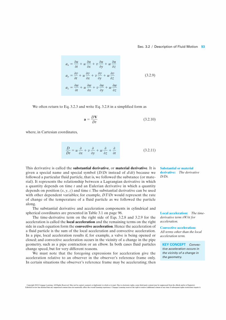
We often return to Eq. 3.2.3 and write Eq. 3.2.8 in a simplified form as
a � �DD
Vt
� (3.2.10)
where, in Cartesian coordinates,
(3.2.11)
This derivative is called the substantial derivative, or material derivative. It isgiven a special name and special symbol (D/Dt instead of d/dt) because wefollowed a particular fluid particle, that is, we followed the substance (or mate-rial). It represents the relationship between a Lagrangian derivative in whicha quantity depends on time t and an Eulerian derivative in which a quantitydepends on position (x, y, z) and time t. The substantial derivative can be usedwith other dependent variables; for example, DT/Dt would represent the rateof change of the temperature of a fluid particle as we followed the particlealong.
The substantial derivative and acceleration components in cylindrical andspherical coordinates are presented in Table 3.1 on page 96.
The time-derivative term on the right side of Eqs. 3.2.8 and 3.2.9 for theacceleration is called the local acceleration and the remaining terms on the rightside in each equation form the convective acceleration. Hence the acceleration ofa fluid particle is the sum of the local acceleration and convective acceleration.In a pipe, local acceleration results if, for example, a valve is being opened orclosed; and convective acceleration occurs in the vicinity of a change in the pipegeometry, such as a pipe contraction or an elbow. In both cases fluid particleschange speed, but for very different reasons.
We must note that the foregoing expressions for acceleration give theacceleration relative to an observer in the observer’s reference frame only.In certain situations the observer’s reference frame may be accelerating; then
�DD
t� � u �
�
�
x� � v �
�
�
y� � „ �
�
�
z� � �
�
�
t�
(3.2.9)
ax � ��
�
ut� � u �
�
�
ux� � v �
�
�
uy� � „ �
�
�
uz�
ay � ��
�
vt� � u �
�
�
xv� � v �
�
�
yv� � „ �
�
�
zv�
az � ��
�
„t� � u �
�
�
„x� � v �
�
�
„y� � „ �
�
�
„z�
Substantial or materialderivative: The derivativeD/Dt.
Local acceleration: The time-derivative term �V/�t foracceleration.
Convective acceleration:All terms other than the localacceleration term.
KEY CONCEPT Convec-tive acceleration occurs inthe vicinity of a change inthe geometry.
Copyright 2010 Cengage Learning. All Rights Reserved. May not be copied, scanned, or duplicated, in whole or in part. Due to electronic rights, some third party content may be suppressed from the eBook and/or eChapter(s). Editorial review has deemed that any suppressed content does not materially affect the overall learning experience. Cengage Learning reserves the right to remove additional content at any time if subsequent rights restrictions require it.
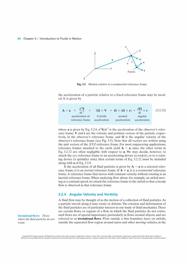
the acceleration of a particle relative to a fixed reference frame may be need-ed. It is given by
(3.2.12)
where a is given by Eq. 3.2.8, d2S/dt 2 is the acceleration of the observer’s refer-ence frame, V and r are the velocity and position vectors of the particle, respec-tively, in the observer’s reference frame, and � is the angular velocity of theobserver’s reference frame (see Fig. 3.5). Note that all vectors are written usingthe unit vectors of the XYZ-reference frame. For most engineering applications,reference frames attached to the earth yield A � a, since the other terms inEq. 3.2.12 are often negligible with respect to a. We may decide, however, toattach the xyz-reference frame to an accelerating device (a rocket), or to a rotat-ing device (a sprinkler arm); then certain terms of Eq. 3.2.12 must be includedalong with a of Eq. 3.2.8.
If the acceleration of all fluid particles is given by A � a in a selected refer-ence frame, it is an inertial reference frame. If A a, it is a noninertial referenceframe. A reference frame that moves with constant velocity without rotating is aninertial reference frame. When analyzing flow about, for example, an airfoil mov-ing at a constant speed, we attach the reference frame to the airfoil so that a steadyflow is observed in that reference frame.
3.2.4 Angular Velocity and Vorticity
A fluid flow may be thought of as the motion of a collection of fluid particles. Asa particle travels along it may rotate or deform. The rotation and deformation ofthe fluid particles are of particular interest in our study of fluid mechanics. Thereare certain flows, or regions of a flow, in which the fluid particles do not rotate;such flows are of special importance, particularly in flows around objects, and arereferred to as irrotational flows. Flow outside a thin boundary layer on airfoils,outside the separated flow region around autos and other moving vehicles, in the
A � a � �ddt
2S2� � 2� � V � � � (� � r) � �
dd�
t� � r
acceleration of Coriolis normal angularreference frame acceleration acceleration acceleration
94 Chapter 3 / Introduction to Fluids in Motion
Particle
r
V
S
Z
Y
X
z
y
x aΩ
Fig. 3.5 Motion relative to a noninertial reference frame.
Irrotational flows: Flowswhere the fluid particles do notrotate.
Copyright 2010 Cengage Learning. All Rights Reserved. May not be copied, scanned, or duplicated, in whole or in part. Due to electronic rights, some third party content may be suppressed from the eBook and/or eChapter(s). Editorial review has deemed that any suppressed content does not materially affect the overall learning experience. Cengage Learning reserves the right to remove additional content at any time if subsequent rights restrictions require it.
Sec. 3.2 / Description of Fluid Motion 95
flow around submerged objects, and many other flows are examples of irrota-tional flows. Irrotational flows are extremely important.
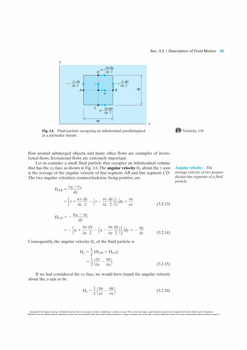
Let us consider a small fluid particle that occupies an infinitesimal volumethat has the xy-face as shown in Fig. 3.6. The angular velocity z about the z-axisis the average of the angular velocity of line segment AB and line segment CD.The two angular velocities, counterclockwise being positive, are
AB � �vB
d
xvA
�
� �v � ��
�
xv� �
d2x� �v �
�
�
xv� �
d2x����dx � �
�
�
xv�
(3.2.13)
CD � �uD
d
yuC
�
� �u � ��
�
u
y� �
d
2
y� �u �
�
�
u
y� �
d
2
y����dy � �
�
�
uy�
(3.2.14)
Consequently, the angular velocity z of the fluid particle is
z � �12
� (�AB � CD)
� �12
� ���
�
xv� �
�
�
uy�� (3.2.15)
If we had considered the xz-face, we would have found the angular velocityabout the y-axis to be
y � �12
� ���
�
uz� �
�
�
„x�� (3.2.16)�
��
�
�
�
�
D
C
BA
y
2+ –– ––dyu u∂
y∂
2– –– ––dyu u∂
y∂
2– –– ––dx∂
x∂ 2+ –– ––dx∂
x∂
x
υ
u
dx
dy
υυ υ υ
Fig. 3.6 Fluid particle occupying an infinitesimal parallelepiped at a particular instant.
Angular velocity: Theaverage velocity of two perpen-dicular line segments of a fluidparticle.
Vorticity, 134
Copyright 2010 Cengage Learning. All Rights Reserved. May not be copied, scanned, or duplicated, in whole or in part. Due to electronic rights, some third party content may be suppressed from the eBook and/or eChapter(s). Editorial review has deemed that any suppressed content does not materially affect the overall learning experience. Cengage Learning reserves the right to remove additional content at any time if subsequent rights restrictions require it.

and the yz-face would provide us with the angular velocity about the x-axis:
�x � �12
� ���
�
„y� �
�
�
zv�� (3.2.17)
These are the three components of the angular velocity vector. A cork placed ina water flow in a wide channel (the xy-plane) would rotate with an angular veloc-ity about the z-axis, given by Eq. 3.2.15.
It is common to define the vorticity � to be twice the angular velocity; itsthree components are then
(3.2.18)
The vorticity components in cylindrical and spherical coordinates are included inTable 3.1 above.
vx � ��
�
„y� �
�
�
zv� vy � �
�
�
uz� �
�
�
„x� vz � �
�
�
xv� �
�
�
uy�
96 Chapter 3 / Introduction to Fluids in Motion
Table 3.1 The Substantial Derivative, Acceleration, and Vorticity in Cartesian, Cylindrical, and Spherical Coordinates
Substantial DerivativeCartesian
�DD
t� � u �
�
�
x� � v �
�
�
y� � „ �
�
�
z� � �
�
�
t�
Cylindrical
�DD
t� � vr �
�
�
r� � �
vru� �
�
�
u� � vz �
�
�
z� � �
�
�
t�
Spherical
�DD
t� � vr �
�
�
r� � �
vru� �
�
�
u� � �
r svif
n u� �
�
�
f� � �
�
�
t�
AccelerationCartesian
ax � ��
�
ut� � u �
�
�
ux� � v �
�
�
uy� � „ �
�
�
uz�
ay � ��
�
vt� � u �
�
�
xv� � v �
�
�
yv� � „ �
�
�
zv�
az � ��
�
„t� � u �
�
�
„x� � v �
�
�
„y� � „ �
�
�
„z�
Cylindrical
ar � ��
�
vtr
� � vr ��
�
vrr
� � �vru� �
�
�
vu
r� � vz �
�
�
vzr
� �vr
2u�
au � ��
�
vtu
� � vr ��
�
vru
� � �vru� �
�
�
vuu
� � vz ��
�
vzu
� � �vr
rvu�
az � ��
�
vtz
� � vr ��
�
vrz
� � �vru� �
�
�
vuz
� � vz ��
�
vzz
�
Spherical
ar � ��
�
vtr
� � vr ��
�
vrr
� � �vru� �
�
�
vu
r� � �
r svif
n u� �
�
�
vf
r� �
vf2 �
rv 2
u�
au � ��
�
vtu
� � vr ��
�
vtu
� � �vru� �
�
�
vuu
� � �r s
vinf
f� �
�
�
vfu
� �
af � ��
�
vtf
� � vr ��
�
vrf
� � �vru� �
�
�
vuf
� � �r s
vif
n u� �
�
�
vff
� �vr vf � vuvf cot u��
r
vrvu vf2 cot u
��r
VorticityCartesian
vx � ��
�
„y� �
�
�
zv� vy � �
�
�
uz� �
�
�
„x� vz � �
�
�
xv� �
�
�
uy�
Cylindrical
vr � �1r
� ���
�
vu
z�� �
�
�
vzu
� vu � ��
�
vzr
� ��
�
vrz
� vz � �1r
� ���(�
rrvu)� �
�
�
vu
r��
Spherical
vr � �r si
1n u� ��
�
�
u� (vf sin u) �
�
�
vfu
�� vf � �1r
� ���
�
r� (rvu) �
�
�
vu
r��
vu � �1r
� ��sin1
u� �
�
�
fvr� �
�
�
r� (rvf)�
Vorticity: Twice the angularvelocity.
Copyright 2010 Cengage Learning. All Rights Reserved. May not be copied, scanned, or duplicated, in whole or in part. Due to electronic rights, some third party content may be suppressed from the eBook and/or eChapter(s). Editorial review has deemed that any suppressed content does not materially affect the overall learning experience. Cengage Learning reserves the right to remove additional content at any time if subsequent rights restrictions require it.

An irrotational flow possesses no vorticity; the cork mentioned above wouldnot rotate in an irrotational flow. We consider this special flow in Section 8.5.
The deformation of the particle of Fig. 3.6 is the rate of change of the anglethat line segment AB makes with line segment CD. If AB is rotating with anangular velocity different from that of CD, the particle is deforming. The defor-mation is represented by the rate-of-strain tensor; its component exy in the xy-plane is given by
exy � �12
� (�AB �CD)
� �12
� ���
�
xv� � �
�
�
uy�� (3.2.19)
For the xz-plane and the yz-plane we have
exz � �12
� ���
�
„x� � �
�
�
uz�� eyz � �
12
� ���
�
„y� � �
�
�
zv�� (3.2.20)
Observe that exy�eyx, exz�ezx, and eyz�ezy. By observation, we see that the rate-of-strain tensor is symmetric.
The fluid particle could also deform by being stretched or compressed in aparticular direction. For example, if point B of Fig. 3.6 is moving faster than pointA, the particle would be stretching in the x-direction. This normal rate of strain ismeasured by
exx � �uB
d
xuA
�
� �u � ��
�
ux� �
d2x� �u �
�
�
ux� �
d2x����dx � �
�
�
ux�
(3.2.21)
Similarly, in the y- and z-directions we would find that
eyy � ��
�
yv� ezz � �
�
�
„z� (3.2.22)
The symmetric rate-of-strain tensor can be displayed as
exx exy exz(3.2.23)eij � �exy eyy eyz�
exz eyz ezz
where the subscripts i and j take on numerical values 1, 2, or 3. Then e12 repre-sents exy in row 1 column 2.
We will see in Chapter 5 that the normal and shear stress components in aflow are related to the foregoing rate-of-strain components. In fact, in the one-dimensional flow of Fig. 1.6, the shear stress was related to �u/�y with Eq. 1.5.5; note that �u/�y is twice the rate-of-strain component given by Eq. 3.2.19with v � 0.
Sec. 3.2 / Description of Fluid Motion 97
Rate-of-strain tensor: Therate at which deformationoccurs.
Copyright 2010 Cengage Learning. All Rights Reserved. May not be copied, scanned, or duplicated, in whole or in part. Due to electronic rights, some third party content may be suppressed from the eBook and/or eChapter(s). Editorial review has deemed that any suppressed content does not materially affect the overall learning experience. Cengage Learning reserves the right to remove additional content at any time if subsequent rights restrictions require it.

Example 3.1The velocity field is given by V � 2x ı yt j m/s, where x and y are in meters and t is inseconds. Find the equation of the streamline passing through (2, 1) and a unit vectornormal to the streamline at (2, 1) at t � 4 s.
SolutionThe velocity vector is tangent to a streamline so that V � dr � 0 (the cross product oftwo parallel vectors is zero). For the given velocity vector we have, at t � 4 s,
(2x ı 4y j) � (dx ı � dy j) � (2x dy � 4y dx)k � 0
where we have used ı � j � k, j � ı � k, and ı � ı � 0. Consequently,
2x dy � 4y dx or �d
y
y� � 2 �
dxx�
Integrate both sides:
ln y � 2 ln x � ln C
where we used ln C for convenience. This is written as
ln y � ln x2 � ln C � ln(Cx2)
Hence
x2y � C
At (2, 1) C � 4, so that the streamline passing through (2, 1) has the equation
x2y � 4
A normal vector is perpendicular to the streamline, hence the velocity vector, so that using n � nx ı � ny j we have at (2, 1) and t � 4 s
V � n � (4 ı � 4 j) � (nx ı � ny j) � 0
Using ı � ı � 1 and ı � j � 0, this becomes
4nx � 4ny � 0 � nx � ny
Then, because n is a unit vector, n2x � n2
y � 1 and we find that
n2x � 1 n2
x � nx � ��
22�
�
The unit vector normal to the streamline is written as
n � ��
22�
� ( ı j)
98 Chapter 3 / Introduction to Fluids in Motion
Copyright 2010 Cengage Learning. All Rights Reserved. May not be copied, scanned, or duplicated, in whole or in part. Due to electronic rights, some third party content may be suppressed from the eBook and/or eChapter(s). Editorial review has deemed that any suppressed content does not materially affect the overall learning experience. Cengage Learning reserves the right to remove additional content at any time if subsequent rights restrictions require it.

Sec. 3.2 / Description of Fluid Motion 99
Example 3.2A velocity field in a particular flow is given by V � 20y2 ı 20xy j m/s. Calculate theacceleration, the angular velocity, the vorticity vector, and any nonzero rate-of-straincomponents at the point (1, 1, 2).
SolutionWe could use Eq. 3.2.9 and find each component of the acceleration, or we could useEq. 3.2.8 and find a vector expression. Using Eq. 3.2.8, we have
0 0
a � u ��
�
Vx� � v �
�
�
Vy� � „ ��
�
Vz� � �
�
�
Vt�
� 20y2( 20y j) 20xy(40y ı 20x j)
� 800xy2 ı 400(y3 x2y) j
where we have used u � 20y2 and v � 20xy, as given by the velocity vector. All par-ticles passing through the point (1, 1, 2) have the acceleration
a � 800 ı m�s2
The angular velocity has two zero components:
0 0 0 0
�x � �12
� ���
�
„y� �
�
�
zv�� � 0, �y � �
12
� ���
�
uz� �
�
�
„x�� � 0
The non-zero z-component is, at the point (1, 1, 2),
�z � �12
� ���
�
xv� �
�
�
uy��
� �12
� (20y 40y) � 30 rad�s
The vorticity vector is twice the angular velocity vector:
� � 2�zk � 60 k rad�s
The nonzero rate-of-strain components are
exy � �12
� ���
�
xv� � �
�
�
uy��
� �12
� (20y � 40y) � 10 rad�s
eyy � ��
�
yv�
� 20x � 20 rad�s
All other rate-of-strain components are zero.
QQQQQQQQO
QQQQQQQQO
QQQQQQQQO
QQQQQQQQO
QQQQQQQQO
QQQQQQQQO
Copyright 2010 Cengage Learning. All Rights Reserved. May not be copied, scanned, or duplicated, in whole or in part. Due to electronic rights, some third party content may be suppressed from the eBook and/or eChapter(s). Editorial review has deemed that any suppressed content does not materially affect the overall learning experience. Cengage Learning reserves the right to remove additional content at any time if subsequent rights restrictions require it.

3.3 CLASSIFICATION OF FLUID FLOWS
In this section we provide an overview of some of the aspects of fluid mechan-ics that are considered in more depth in subsequent sections and chapters.Although most of the notions presented here are redefined and discussed indetail later, it will be helpful at this point to introduce the general classificationof fluid flows.
3.3.1 One-, Two-, and Three-Dimensional Flows
In the Eulerian description of motion the velocity vector, in general, depends onthree space variables and time, that is, V � V(x, y, z, t). Such a flow is a three-dimensional flow, because the velocity vector depends on three space coordi-nates. The solutions to problems in such a flow are very difficult and are beyondthe scope of an introductory course. Even if the flow could be assumed to besteady [i.e., V � V(x, y, z)], it would remain a three-dimensional flow. A particu-lar flow is shown in Fig. 3.7. This flow is normal to a plane surface; the fluiddecelerates and comes to rest at the stagnation point. The velocity components,u, v, and „ depend on x, y and z; that is, u � u(x, y, z), v � v(x, y, z) and „ � „(x, y, z).
Often a three-dimensional flow can be approximated as a two-dimensionalflow. For example, the flow over a wide dam is three-dimensional because of theend conditions, but the flow in the central portion away from the ends can betreated as two-dimensional. In general, a two-dimensional flow is a flow in whichthe velocity vector depends on only two space variables. An example is a planeflow, in which the velocity vector depends on two spatial coordinates, x and y, butnot z, i.e., V � V(x, y). In an axisymmetric flow, the velocity vector would dependin r and , i.e., V = V(r, ); the flow in Fig. 3.7 will be considered two dimension-al if described in a cylindrical coordinate system.
A one-dimensional flow is a flow in which the velocity vector depends ononly one space variable. Such flows occur away from geometry changes in
uuOne-dimensional flow: Thevelocity vector depends ononly one space variable.
100 Chapter 3 / Introduction to Fluids in Motion
Stagnationpoint
V
z
x(V = 0)
V
Fig. 3.7 A stagnation point flow.
Three-dimensional flow: Thevelocity vector depends onthree space variables.
Stagnation point: The pointwhere the fluid comes to rest.
Two-dimensional flow: Thevelocity vector is dependent ononly two space variables.
Plane flow: The velocityvector depends on the twocoordinates x and y.
Copyright 2010 Cengage Learning. All Rights Reserved. May not be copied, scanned, or duplicated, in whole or in part. Due to electronic rights, some third party content may be suppressed from the eBook and/or eChapter(s). Editorial review has deemed that any suppressed content does not materially affect the overall learning experience. Cengage Learning reserves the right to remove additional content at any time if subsequent rights restrictions require it.

Sec. 3.3 / Classification of Fluid Flows 101
long, straight pipes or between parallel plates, as shown in Fig. 3.8. The veloc-ity in the pipe varies only with r, i.e., u � u(r). The velocity between parallelplates varies only with the coordinate y, i.e., u � u(y). Even if the flow isunsteady so that u � u(y, t), as would be the situation during startup, the flowis one-dimensional.
The flows shown in Fig. 3.8 may also be referred to as developed flows; thatis, the velocity profile does not vary with respect to the space coordinate in thedirection of flow. This demands that the region of interest be a substantial dis-tance from an entrance or a sudden change in geometry.
There are many engineering problems in fluid mechanics in which a flowfield is simplified to a uniform flow: the velocity, and other fluid properties, areconstant over the area, as in Fig. 3.9. This simplification is made when the velo-city is essentially constant over the area, a rather common occurrence. Examplesof such flows are relatively high speed flow in a pipe section, and flow in a stream.The average velocity may change from one section to another; the flow condi-tions depend only on the space variable in the flow direction. For large conduits,however, it may be necessary to consider hydrostatic variation in the pressurenormal to the streamlines.
3.3.2 Viscous and Inviscid Flows
A fluid flow may be broadly classified as either a viscous flow or an inviscid flow.An inviscid flow is one in which viscous effects do not significantly influence theflow and are thus neglected. In a viscous flow the effects of viscosity are impor-tant and cannot be ignored.
To model an inviscid flow analytically, we can simply let the viscosity be zero;this will obviously make all viscous effects zero. It is more difficult to create aninviscid flow experimentally, because all fluids of interest (such as water and air)
u(r ) u(y)
(a) (b)
r
x
y
x
Fig. 3.8 One-dimensional flow: (a) flow in a pipe;(b) flow between parallel plates.
V1V2
Fig. 3.9 Uniform velocity profiles.
Inviscid flow: Viscous effectsdo not significantly influencethe flow.
Viscous flow: The effects ofviscosity are significant.
Uniform flow: The fluidproperties are constant over thearea.
Developed flows: Thevelocity profile does not varywith respect to the spacecoordinate in the direction offlow.
Copyright 2010 Cengage Learning. All Rights Reserved. May not be copied, scanned, or duplicated, in whole or in part. Due to electronic rights, some third party content may be suppressed from the eBook and/or eChapter(s). Editorial review has deemed that any suppressed content does not materially affect the overall learning experience. Cengage Learning reserves the right to remove additional content at any time if subsequent rights restrictions require it.

have viscosity. The question then becomes: Are there flows of interest in whichthe viscous effects are negligibly small? The answer is “yes, if the shear stresses inthe flow are small and act over such small areas that they do not significantlyaffect the flow field.” This statement is very general, of course, and it will takeconsiderable analysis to justify the inviscid flow assumption.
Based on experience, it has been found that the primary class of flows, whichcan be modeled as inviscid flows, is external flows, that is, a flow which existsexterior to bodies. Inviscid flows are of primary importance in flows aroundstreamlined bodies, such as flow around an airfoil or a hydrofoil. Any viscouseffects that may exist are confined to a thin layer, called a boundary layer, whichis attached to the boundary, such as that shown in Fig. 3.10; the velocity in aboundary layer is always zero at a fixed wall, a result of viscosity. For many flowsituations, boundary layers are so thin that they can simply be ignored whenstudying the gross features of a flow around a streamlined body. For example, theinviscid flow solution provides an excellent prediction to the flow around the air-foil, except inside the boundary layer and possibly near the trailing edge. Inviscidflow is also encountered in contractions inside piping systems and in shortregions of internal flows where viscous effects are negligible.
Viscous flows include the broad class of internal flows, such as flows in pipesand conduits and in open channels. In such flows viscous effects cause substantial“losses” and account for the huge amounts of energy that must be used totransport oil and gas in pipelines. The no-slip condition resulting in zero velocityat the wall and the resulting shear stresses lead directly to these losses.
3.3.3 Laminar and Turbulent Flows
A viscous flow can be classified as either a laminar flow or a turbulent flow. In alaminar flow the fluid flows with no significant mixing of neighboring fluid parti-cles. If dye were injected into the flow, it would not mix with the neighboring fluidexcept by molecular activity; it would retain its identity for a relatively long pe-riod of time.Viscous shear stresses always influence a laminar flow.The flow maybe highly time dependent, due to the erratic motion of a piston as shown by theoutput of a velocity probe in Fig. 3.11a, or it may be steady, as shown in Fig. 3.11b.
102 Chapter 3 / Introduction to Fluids in Motion
External flows: Flows thatexist exterior to bodies.
Boundary layer: A thin layerattached to the boundary inwhich viscous effects areconcentrated.
Inviscidflow
Boundarylayer
Edge ofboundary
layer
Fig. 3.10 Flow around an airfoil.
KEY CONCEPT Inviscidflow provides an excellentprediction to the flowaround an airfoil.
Laminar flow: A flow withno significant mixing ofparticles but with significantviscous shear stresses.
Inviscid flow, 164
Motion near a boundary,159
Copyright 2010 Cengage Learning. All Rights Reserved. May not be copied, scanned, or duplicated, in whole or in part. Due to electronic rights, some third party content may be suppressed from the eBook and/or eChapter(s). Editorial review has deemed that any suppressed content does not materially affect the overall learning experience. Cengage Learning reserves the right to remove additional content at any time if subsequent rights restrictions require it.

Sec. 3.3 / Classification of Fluid Flows 103
In a turbulent flow fluid motions vary irregularly so that quantities such asvelocity and pressure show a random variation with time and space coordinates.The physical quantities are often described by statistical averages. In this sensewe can define a “steady” turbulent flow as a flow in which the time-average phys-ical quantities do not change in time. Figure 3.12 shows instantaneous velocitymeasurements in an unsteady and a steady turbulent flow. A dye injected into aturbulent flow would mix immediately by the action of the randomly movingfluid particles; it would quickly lose its identity in this diffusion process.
A laminar flow and a turbulent flow can be observed by performing a simpleexperiment with a water faucet. Turn the faucet on so the water flows out veryslowly as a silent stream.This is laminar flow. Open the faucet slowly and observethe flow becoming turbulent. Note that a turbulent flow develops with a rela-tively small flow rate.
The reason why a flow can be laminar or turbulent has to do with what hap-pens to a small flow disturbance, a perturbation to the velocity components. Aflow disturbance can either increase or decrease in size. If a flow disturbance ina laminar flow increases (i.e., the flow is unstable), the flow may become turbu-lent; if the disturbance decreases, the flow remains laminar. In certain situationsthe flow may develop into a different laminar flow, as is the case between con-centrically rotating cylinders shown in Fig. 3.13. At low rotational speed the flowwould be in simple circles. But at a sufficiently high speed the flow becomesunstable and the vortices suddenly appear; it is a much more complex laminarflow called Taylor-Conette flow.
V(t) V(t)
t
(a)
t
(b)
Fig. 3.11 Velocity as a function of time in a laminar flow: (a) unsteady flow;(b) steady flow.
t
V(t)
(a)t
V(t)
(b)
Fig. 3.12 Velocity as a function of time in a turbulent flow: (a) unsteady flow;(b) “steady” flow.
Turbulent flow: Flow variesirregularly so that flowquantities show randomvariation.
KEY CONCEPT A dyeinjected into a turbulentflow would miximmediately.
Copyright 2010 Cengage Learning. All Rights Reserved. May not be copied, scanned, or duplicated, in whole or in part. Due to electronic rights, some third party content may be suppressed from the eBook and/or eChapter(s). Editorial review has deemed that any suppressed content does not materially affect the overall learning experience. Cengage Learning reserves the right to remove additional content at any time if subsequent rights restrictions require it.

Whether a flow is laminar or turbulent depends on three physical parametersdescribing the flow conditions. The first parameter is a length scale of the flowfield, such as the thickness of a boundary layer or the diameter of a pipe. If thislength scale is sufficiently large, a flow may be turbulent. The second parameteris a velocity scale such as a spatial average of the velocity; for a large enoughvelocity the flow may be turbulent. The third parameter is the kinematic viscosi-ty; for a small enough viscosity the flow may be turbulent.
The three parameters can be combined into a single parameter that can serveas a tool to predict the flow regime.This quantity is the Reynolds number, namedafter Osborne Reynolds (1842–1912), a dimensionless parameter, defined as
Re � �VnL� (3.3.1)
where L and V are a characteristic length and velocity, respectively, and n is thekinematic viscosity; for example, in a pipe flow L would be the pipe diameter andV would be the average velocity. If the Reynolds number is relatively small, theflow is laminar as shown in Figs. 3.13 and 3.14; if it is large, the flow is turbulent.This is more precisely stated by defining a critical Reynolds number, Recrit, sothat the flow is laminar if Re Recrit. For example, in a flow inside a rough-walled pipe it is found that Recrit � 2000. This is the minimum critical Reynoldsnumber and is used for most engineering applications. If the pipe wall is ex-tremely smooth and free of vibration, the critical Reynolds number can be
104 Chapter 3 / Introduction to Fluids in Motion
Reynolds number:Parameter combining a lengthscale, a velocity scale, and thekinematic viscosity into
Critical Reynolds number:The number above which aprimary laminar flow ceases toexist.
Re � VL/v
Fig. 3.13 Laminar flowbetween rotating cylinders. Asecondary flow occurs as regu-larly spaced toroidal vortices.(“Steady supercritical Taylorvortex flow,” by Burkhalterand Koschmieder. FromJournal of Fluid Mechanicsvol. 58, pp. 547–560 (1973).2006 © Cambridge Journals,reproduced with permission.)
Fig. 3.14 Streamlines around a semicircular arc. At this Reynolds number of 0.031 thecenters of the pair of eddies in the cavity are separated by 0.52 diameter, in good agree-ment with an analytical solution. Aluminum powder dispersed in glycerine is illuminatedby a slit of light. (Photograph by Sadatoshi Taneda. From Album of Fluid Motion, 1982,The Parabolic Press, Stanford, California.)
Taylor cells, 24
Copyright 2010 Cengage Learning. All Rights Reserved. May not be copied, scanned, or duplicated, in whole or in part. Due to electronic rights, some third party content may be suppressed from the eBook and/or eChapter(s). Editorial review has deemed that any suppressed content does not materially affect the overall learning experience. Cengage Learning reserves the right to remove additional content at any time if subsequent rights restrictions require it.

Sec. 3.3 / Classification of Fluid Flows 105
increased as the fluctuation level in the flow is decreased; values in excess of 40 000 have been measured. The critical Reynolds number is different for everygeometry, e.g., it is 1500 for flow between parallel plates using the averagevelocity and the distance between the plates.
The flow can also be intermittently turbulent and laminar; this is called anintermittent flow.This phenomenon can occur when the Reynolds number is closeto Recrit. Figure 3.15 shows the output of a velocity probe for such a flow.
In a boundary layer that exists on a flat plate, due to a constant-velocity fluidstream, as shown in Fig. 3.16, the length scale changes with distance from theupstream edge. A Reynolds number is calculated using the length x as the char-acteristic length. For a certain xT, Re becomes Recrit and the flow undergoes tran-sition from laminar to turbulent. For a smooth rigid plate in a uniform flow witha low free-stream fluctuation level, values as high as Recrit � 106 have beenobserved. In most engineering applications we assume a rough wall, or high free-stream fluctuation level, with an associated critical Reynolds number of approx-imately 3 � 105.
It is not appropriate to refer to an inviscid flow as laminar or as turbulent.The inviscid flow of Fig. 3.10 is often called the free stream. The free stream canbe irrotational or it can possess vorticity; most often it is irrotational.
t
V(t)
Fig. 3.15 Velocity versus time signal from a velocity probe in an intermittent flow.
Laminarflow
Transition
xT
V
x
Turbulentflow
Fig. 3.16 Boundary layer flow on a flat plate.
KEY CONCEPT In mostapplications, we assume acritical Reynolds number of3 � 105 in flow on a flatplate.
Free stream: The inviscidflow outside the boundarylayer in an external flow.
Reynolds number, 524
Pipe flow, 202
Copyright 2010 Cengage Learning. All Rights Reserved. May not be copied, scanned, or duplicated, in whole or in part. Due to electronic rights, some third party content may be suppressed from the eBook and/or eChapter(s). Editorial review has deemed that any suppressed content does not materially affect the overall learning experience. Cengage Learning reserves the right to remove additional content at any time if subsequent rights restrictions require it.

Example 3.3The 2-cm-diameter pipe of Fig. E3.3 is used to transport water at 20°C. What is the maximum average velocity that may exist in the pipe for which laminar flow isguaranteed?
Fig. E3.3
SolutionThe kinematic viscosity is found in Appendix B to be n � 106 m2/s. Using a Reynoldsnumber of 2000 so that a laminar flow is guaranteed, we find that
V � �20
D00n�
� �2000
0�
.02106
� � 0.1 m�s
This average velocity is quite small. Velocities this small are not usually encountered inactual situations; hence laminar flow is seldom of engineering interest except for spe-cialized topics such as lubrication. Most internal flows are turbulent flows, and thus thestudy of turbulence gains much attention.
3.3.4 Incompressible and Compressible Flows
The last major classification of fluid flows to be considered in this chapter sepa-rates flows into incompressible and compressible flows. An incompressible flowexists if the density of each fluid particle remains relatively constant as it movesthrough the flow field, that is,
(3.3.2)
This does not demand that the density is everywhere constant. If the density isconstant, then obviously, the flow is incompressible, but that would be a morerestrictive condition.Atmospheric flow, in which r � r(z), where z is vertical, andflows that involve adjacent layers of fresh and salt water, as happens when riversenter the ocean, are examples of incompressible flows in which the density varies.
In addition to liquid flows, low-speed gas flows, such as the atmospheric flowreferred to above, are also considered to be incompressible flows. The Machnumber, named after Ernst Mach (1838–1916), is defined as
(3.3.3)M � �Vc
�
�D
D
r
t� � 0
V
Water @ 20°C
106 Chapter 3 / Introduction to Fluids in Motion
Incompressible flow: Thedensity of each fluid particleremains constant.
KEY CONCEPT Constantdensity is more restrictivethan incompressibility.
Mach number: A parameterin a gas flow defined as M � V/c.
Copyright 2010 Cengage Learning. All Rights Reserved. May not be copied, scanned, or duplicated, in whole or in part. Due to electronic rights, some third party content may be suppressed from the eBook and/or eChapter(s). Editorial review has deemed that any suppressed content does not materially affect the overall learning experience. Cengage Learning reserves the right to remove additional content at any time if subsequent rights restrictions require it.

where V is the gas speed and the wave speed c � �kRT� . Equation 3.3.3 is use-ful in deciding whether a particular gas flow can be studied as an incompressibleflow. If M 0.3, density variations are at most 3% and the flow is assumed tobe incompressible; for standard air this corresponds to a velocity below about100 m/s or 300 ft/sec. If M � 0.3, the density variations influence the flow andcompressibility effects should be accounted for; such flows are compressibleflows and are considered in Chapter 9.
Incompressible gas flows include atmospheric flows, the aerodynamics oflanding and takeoff of commercial aircraft, heating and air-conditioning airflows,flow around automobiles and through radiators, and the flow of air around build-ings, to name a few. Compressible flows include the aerodynamics of high-speedaircraft, airflow through jet engines, steam flow through the turbine in a powerplant, airflow in a compressor, and the flow of the air-gas mixture in an internalcombustion engine.
3.4 THE BERNOULLI EQUATION
In this section we present an equation that is probably used more often in fluidflow applications than any other equation. It is also often misused; it is thusimportant to understand its limitations. Its limitations are a result of severalassumptions made in the derivation. One of the assumptions is that viscouseffects are neglected. In other words, in view of Eq. 1.5.5, shear stressesintroduced by velocity gradients are not taken into consideration. These stressesare often very small compared with pressure differences in the flow field. Locally,these stresses have little effect on the flow field and the assumption is justified.However, over long distances or in regions of high-velocity gradients, thesestresses may affect the flow conditions so that viscous effects must be included.
The derivation of this important equation, the Bernoulli equation, starts withthe application of Newton’s second law to a fluid particle. Let us use an infini-tesimal cylindrical particle positioned as shown in Fig. 3.17, with length ds andcross-sectional area dA. The forces acting on the particle are the pressure forcesand the weight, as shown. Summing forces in the direction of motion, the s-direc-tion, there results
p dA �p � ��
�
p
s� ds� dA rg ds dA cos u � r ds dA as (3.4.1)
where as is the acceleration of the particle in the s-direction. It is given by1
as � V ��
�
Vs� � �
�
�
Vt� (3.4.2)
where �V/�t � 0 since we will assume steady flow. Also, we see that
dh � ds cos u � ��
�
hs� ds (3.4.3)
so that
cos u � ��
�
hs� (3.4.4)
Sec. 3.4 / The Bernoulli Equation 107
1 This can be verified by considering Eq. 3.2.9a, assuming that v � „ � 0. Think of the x-direction being tangent tothe streamline at the instant shown, so that u � V.
Compressible flow: Densityvariations influence the flow.
KEY CONCEPT Shearstresses are often verysmall compared withpressure differences.
Copyright 2010 Cengage Learning. All Rights Reserved. May not be copied, scanned, or duplicated, in whole or in part. Due to electronic rights, some third party content may be suppressed from the eBook and/or eChapter(s). Editorial review has deemed that any suppressed content does not materially affect the overall learning experience. Cengage Learning reserves the right to remove additional content at any time if subsequent rights restrictions require it.

Then, after dividing by ds dA, and using the above equations for as and cos u,Eq 3.4.1 takes the form
��
�
p
s� rg �
�
�
hs� � rV �
�
�
Vs� (3.4.5)
Now, we assume constant density and note that V�V/�s � �(V2/2)/�s; then we canwrite Eq. 3.4.5 as
��
�
s� ��
V2
2
� � �p
r� � gh� � 0 (3.4.6)
This is satisfied if, along the streamline,
�V2
2
� � �p
r� � gh � const (3.4.7)
where the constant may have a different value on a different streamline. Betweentwo points on the same streamline,
(3.4.8)
This is the well-known Bernoulli equation, named after Daniel Bernoulli(1700–1782). Note the five assumptions:
–Inviscid flow (no shear stresses)–Steady flow (�V/�t � 0)–Along a streamline (as � V�V/�s)–Constant density (�r/�s � 0)–Inertial reference frame (A � a as in Eq. 3.2.12)
If Eq. 3.4.8 is divided by g, the dimension of each term is length andBernoulli’s equation takes the alternate form
�V
2
21
� � �p
r1� � gh1 � �
V
2
22
� � �p
r2� � gh2
108 Chapter 3 / Introduction to Fluids in Motion
Streamline
n
s
y
p dA
dA
dsV
g ds dAρ
θ R (radius of curvature)
p + –– ds dAps( (
dh = –– ds
x
∂∂
hs
∂∂
Fig. 3.17 Particle moving along a streamline.
Bernoulli’s equation, 910
Copyright 2010 Cengage Learning. All Rights Reserved. May not be copied, scanned, or duplicated, in whole or in part. Due to electronic rights, some third party content may be suppressed from the eBook and/or eChapter(s). Editorial review has deemed that any suppressed content does not materially affect the overall learning experience. Cengage Learning reserves the right to remove additional content at any time if subsequent rights restrictions require it.

Sec. 3.4 / The Bernoulli Equation 109
(3.4.9)
The sum of the two terms (p/g � h) is called the piezometric head and the sum ofthe three terms the total head. The pressure p is often referred to as static pres-sure, and the sum of the two terms
p � r �V2
2
� � pT (3.4.10)
is called the total pressure pT or stagnation pressure, the pressure at a stagnationpoint (see Fig. 3.7) in the flow.
The static pressure in a pipe can be measured simply by installing a so-calledpiezometer, shown2 in Fig. 3.18a. A device, known as a pitot probe, sketched inFig. 3.18b, is used to measure the total pressure in a fluid flow. Point 2 just insidethe pitot tube is a stagnation point; the velocity there is zero. The differencebetween the readouts can be used to determine the velocity at point 1. A pitot-static probe is also used to measure the difference between total and static pres-sure with one probe (Fig. 3.18c). The velocity at point 1 (using the readings of thepiezometer and pitot probes, or the reading from the pitot-static probe) can bedetermined by applying the Bernoulli equation between points 1 and 2:
�V
2g
21
� � �p
g1� � �
p
g2� (3.4.11)
where we have assumed point 2 to be a stagnation point so that V2 � 0.This gives
V1 � ��2r
� (p2� p1)� (3.4.12)
We will find many uses for Bernoulli’s equation in our study of fluids. Wemust be careful, however, never to use it in an unsteady flow or if viscous effectsare significant (the primary reasons for making Bernoulli’s equation inapplica-ble). We must also never confuse Bernoulli’s equation with the energy equation;they are independent equations as Example 3.6 illustrates.
�V2g
21� � �
p
g1� � h1 � �
V2g
22� � �
p
g2� � h2
p2(total pressure)
p1(static pressure)
V
p2 _ p1
Static pressureopening
1 2
(a) (b) (c)
Fig. 3.18 Pressure probes: (a) piezometer; (b) pitot probe; (c) pitot-static probe.
Static pressure: The pressurep, usually expressed as gagepressure.
Stagnation pressure: Thepressure that exists at astagnation point.
Piezometer: Gauge designedto measure static pressure.
Pitot probe: Gauge designedto measure total pressure.
Pitot-static probe: Gaugedesigned to measure thedifference between total andstatic pressure.
KEY CONCEPT The totalpressure is p � rV2/2.
KEY CONCEPT Neverconfuse Bernoulli’sequations with the energyequation.
2 When drilling the hole in the wall necessary for the piezometer, burrs are often formed on the inner surface. It isimportant that such burrs be removed since they may cause errors as high as 30% in the pressure reading.
Copyright 2010 Cengage Learning. All Rights Reserved. May not be copied, scanned, or duplicated, in whole or in part. Due to electronic rights, some third party content may be suppressed from the eBook and/or eChapter(s). Editorial review has deemed that any suppressed content does not materially affect the overall learning experience. Cengage Learning reserves the right to remove additional content at any time if subsequent rights restrictions require it.

The Bernoulli equation can be used to determine how high the water from afireman’s hose will reach, to find the pressure on the surface of a low-speed air-foil,3 and to find the wind force on the window in a house. These examples are allexternal flows, flows around objects submerged in the fluid.
Another class of problems where inviscid flow can be assumed and wherethe Bernoulli equation finds frequent application involves internal flows over rel-atively short distances, for example, flow through a contraction, as shown inFig. 3.19a, or flow from a plenum, as shown in Fig. 3.19b. For a given velocity pro-file entering the short contraction, the pressure drop ( p1 p2) and the velocityprofile at section 2 can be approximated assuming an inviscid flow. Viscouseffects are typically very small and require substantial distances and areas overwhich to operate in order to become significant; so in situations such as thoseshown in Fig. 3.19, viscous effects can often be neglected.
Inviscid flow does not always give a good approximation to the actual flowthat exists around a body. Consider the inviscid flow around the sphere (or cylin-der), shown in Fig. 3.20. A stagnation point where V � 0 exists at both the frontand the back of the sphere. Bernoulli’s equation predicts a maximum pressureat the stagnation points A and C because the velocity is zero at such points. Amaximum velocity, and thus a minimum pressure, would exist at point B. In
110 Chapter 3 / Introduction to Fluids in Motion
3 To consider the flow around an aircraft as a steady flow, we simply make the aircraft stationary and move theair, as is done in model studies using a wind tunnel. The pressures and forces remain unchanged.
(b)
p2
(a)
p1V1 = 0~
p1p2
Fig. 3.19 Internal inviscid flows: (a) flow through a contraction; (b) flow from a plenum.
Separatedregion
(a) (b)
Thin boundarylayer
Flowseparates
ACA
B B
Fig. 3.20 Flow around a sphere: (a) inviscid flow; (b) actual flow.
KEY CONCEPT Viscouseffects require substantialareas in order to besignificant.
Flow over a cylinder, 95
Flow over a cylinder, 190
Copyright 2010 Cengage Learning. All Rights Reserved. May not be copied, scanned, or duplicated, in whole or in part. Due to electronic rights, some third party content may be suppressed from the eBook and/or eChapter(s). Editorial review has deemed that any suppressed content does not materially affect the overall learning experience. Cengage Learning reserves the right to remove additional content at any time if subsequent rights restrictions require it.

Sec. 3.4 / The Bernoulli Equation 111
the inviscid flow of part (a), the fluid flowing from B to C must flow from the low-pressure region near B to the high-pressure region near C. In the actual flowthere exists a thin boundary layer in which the velocity goes to zero at the sur-face of the sphere. This slow-moving fluid near the boundary does not have suf-ficient momentum to move into the higher-pressure region near C; the result isthat the fluid separates from the boundary—the boundary streamline leaves theboundary—creating a separated region, a region of recirculating flow, as shownin the actual flow sketched in part (b). The pressure does not increase butremains relatively low over the rear part of the sphere. The high pressure thatexists near the front stagnation point is never recovered on the rear of the sphere,resulting in a relatively large drag force in the direction of flow. A similar situa-tion occurs in the flow around an automobile.
The flow on the front of the sphere is well approximated by an inviscid flow,but it is obvious that the flow over the rear of the sphere deviates radically froman inviscid flow. Viscous effects in the boundary layer have led to a separatedflow, a phenomenon that is often undesirable. For example, separated flow on anairfoil is called stall and must never occur, except on the wings of special stuntplanes. On the blades of a turbine separated flows lead to substantially reducedefficiency. The air deflector on the roof of the cab of a semitruck reduces the sep-arated region, thereby reducing drag and fuel consumption.
If viscous effects are negligible in a steady liquid flow, we can use Bernoulli’sequation to locate points of possible cavitation. This condition occurs when the local pressure becomes equal to the vapor pressure of the liquid. It is to beavoided, if at all possible, because of damage to solid surfaces or because the vapor-ized liquid may cause devices to not operate effectively. Figure 3.21 shows cavitat-ing flow just downstream of a contraction in a pipe. At the point where cavitationoccurs, small vapor bubbles are generated, and these bubbles collapse when theyenter a higher-pressure region.The collapse is accompanied by very large local pres-sures that last for only a small fraction of a second.These pressure spikes may reacha wall, where they can, after repeated applications, result in significant damage.
An important observation regarding pressure changes in a fluid needs to bemade regarding entrances and exits to a pipe or conduit. Consider a flow from areservoir through a pipe, as sketched in Fig. 3.22. At the entrance the streamlinesare curved and the pressure is not constant across section 1, so the pressure atsection 1 cannot be assumed to be uniform. At the exit, however, the streamlines
Fig. 3.21 Cavitation in a nozzle, with water flowing at a velocity of 15 m/s: (a) incandes-cent lamp, exposure time �
310� s; (b) strobe light exposure time 5 ms. (Photograph courtesy of
the Japan Society of Mechanical Engineers and Pergamon Press.)
(a) (b)
Separated region: A regionof recirculating flow due to thefluid separating from theboundary.
KEY CONCEPT Pressureremains relatively low overthe rear part of a sphere.
KEY CONCEPT The flowon the front of a sphere isapproximated by an inviscidflow.
Stall: Separated flow on anairfoil.
KEY CONCEPTCavitation occurs when thelocal pressure equals thevapor pressure.
KEY CONCEPT At a pipeentrance, the streamlinesare curved and the pressureis not constant across theinlet area.
Flow past a cylinder, 166
Copyright 2010 Cengage Learning. All Rights Reserved. May not be copied, scanned, or duplicated, in whole or in part. Due to electronic rights, some third party content may be suppressed from the eBook and/or eChapter(s). Editorial review has deemed that any suppressed content does not materially affect the overall learning experience. Cengage Learning reserves the right to remove additional content at any time if subsequent rights restrictions require it.
are straight, so that no acceleration exists normal to the streamlines; hence thepressure forces acting on the ends of the small cylindrical control volume mustbe equal. We write this as p2 � patm or p2 � 0 gage pressure.
In Fig. 3.17 we summed forces on the fluid element along the streamline andderived Bernoulli’s equation. We can gain additional insight into the pressurefield if we sum forces normal to the streamline. Let us consider the fluid particleto be a parallelepiped with thickness dn in the n-direction and area dAs on theside with length ds. Applying Newton’s second law in the n-direction provides
pdAs �p � ��
�
p
n� dn�dAs � rdAsdn �
VR
2
� (3.4.13)
where we have neglected the weight since we are not intending to integrate oversignificant distances. We have assumed the acceleration in the normal directionto be V2/R, where R is the radius of curvature in this plane flow (in a three-dimensional flow there would be a principal radius of curvature and a binormalradius of curvature). Equation (3.4.13) reduces to
��
�
p
n� � r �
VR
2
� (3.4.14)
From this equation we can qualitatively describe how the pressure changes nor-mal to a streamline (Bernoulli’s equation predicts the pressure changes along astreamline). If we replace �p/�n with �p/�n, the incremental pressure change �pover the short distance �n normal to the streamline is given by
(3.4.15)
This says that the pressure decreases in the n-direction; this decrease is directlyproportional to r and V 2 and inversely proportional to R. Consequently, a tor-nado, with p � 0 outside the tornado, will have a very low pressure at its centerwhere R is relatively small and V is quite large.
In Fig. 3.22 the pressure would be relatively low at the corner of section 1 andrelatively high at the center of section 1. Such qualitative descriptions can bequite helpful in understanding fluid flow behavior.
�p � r �VR
2
� �n
112 Chapter 3 / Introduction to Fluids in Motion
1
2
patmA
p2A
Fig. 3.22 Exit flow into the atmosphere.
KEY CONCEPT Thepressure decreases in the n-direction.
Copyright 2010 Cengage Learning. All Rights Reserved. May not be copied, scanned, or duplicated, in whole or in part. Due to electronic rights, some third party content may be suppressed from the eBook and/or eChapter(s). Editorial review has deemed that any suppressed content does not materially affect the overall learning experience. Cengage Learning reserves the right to remove additional content at any time if subsequent rights restrictions require it.

Sec. 3.4 / The Bernoulli Equation 113
Example 3.4The wind reaches a speed of 90 mph in a storm. Calculate the force acting on the3 ft � 6 ft window of Fig. E3.4 facing the storm. The window is in a high-rise building,so the wind speed is not reduced due to ground effects. Use r � 0.0024 slug/ft3.
Fig. E3.4
SolutionThe window facing the storm will be in a stagnation region where the wind speed isbrought to zero. Working with gage pressures, the pressure p upstream in the wind iszero. The velocity V must have units of ft/sec. It is
V � 90 �mhr
i� � �
36100
hrsec
� � �52
18m0
ift
� � 132 ft�sec
Bernoulli’s equation can be used in this situation since we can neglect viscous effects,and steady flow occurs along a streamline at constant density (air is incompressible atspeeds below about 220 mph). We calculate the pressure on the window selecting state 1in the free stream and state 2 on the window, as follows:
�V
2g
21
� � �p
g1� � h1 � �
V
2g
22
� � �p
g2� � h2
0 0
� p2 � �rV
2
21
�
� 20.9 lb�ft2
where we have used g � rg, h2 � h1, p1 � 0, and V2 � 0. Multiply by the area and findthe force to be
F � pA
� 20.9 � 3 � 6 � 376 lb
We recommend that you verify the units of lb/ft2 on the pressure calculation above. Todo this, use F � ma which provides slug � lb � sec2/ft. When using English units, alwaysuse mass in slugs, length in feet, force in pounds, and time in seconds.
� 0.0024 slug/ft3 � 13.22 ft2/sec2
2
V = 65 mph
Window
QQQQQQQQO
QQQQQQQQO
Copyright 2010 Cengage Learning. All Rights Reserved. May not be copied, scanned, or duplicated, in whole or in part. Due to electronic rights, some third party content may be suppressed from the eBook and/or eChapter(s). Editorial review has deemed that any suppressed content does not materially affect the overall learning experience. Cengage Learning reserves the right to remove additional content at any time if subsequent rights restrictions require it.

Example 3.5The static pressure head in an air pipe (Fig. E3.5) is measured with a piezometer as16 mm of water. A pitot probe indicates 24 mm of water. Calculate the velocity ofthe 20°C air.Also, calculate the Mach number and comment as to the compressibility ofthe flow.
Fig. E3.5
SolutionBernoulli’s equation is applied between two points on the streamline that terminatesat the stagnation point of the pitot probe. Point 1 is upstream and p2 is the total pres-sure at point 2; then, with no elevation change,
�V
2g
21
� � �p
g1� � �
p
gT�
The pressure measured with the piezometer is p1 � gh � 9810 � 0.016 � 157 Pa. Weuse the ideal gas law to calculate the density:
r � �R
p
T�
where standard atmospheric pressure, which is 101 000 Pa (if no elevation is given,assume standard conditions), is added since absolute pressure is needed in the ideal gaslaw. The units are checked by using Pa � N/m2 and J � N�m. The velocity is then
V1 � ��2r
� (pT� p1)�� � 11.42 m�s
where the units can be verified by using kg � N�s2/m. To find the Mach number, wemust calculate the speed of sound. From Eq. 1.7.17 it is
c � �kRT�
�
The Mach number is then
M � �Vc
� � �1314.434
� � 0.0334
Obviously, the flow can be assumed to be incompressible since M 0.3. The velocitywould have to be much higher before compressibility would be significant.
21.4 � 287 kJ/kg�K � 293 K � 343 m/s
B2(0.024 � 9810 157) Pa
1.203 kg/m3
�(157 � 101 000)Pa
287 kJ/kg�K � (273 � 20)K� 1.203 kg/m3
V
24 mm H2O
20° air21
16 mm H2O
114 Chapter 3 / Introduction to Fluids in Motion
Copyright 2010 Cengage Learning. All Rights Reserved. May not be copied, scanned, or duplicated, in whole or in part. Due to electronic rights, some third party content may be suppressed from the eBook and/or eChapter(s). Editorial review has deemed that any suppressed content does not materially affect the overall learning experience. Cengage Learning reserves the right to remove additional content at any time if subsequent rights restrictions require it.

Sec. 3.4 / The Bernoulli Equation 115
Example 3.6Bernoulli’s equation, in the form of Eq. 3.4.8, looks very much like the energy equationdeveloped in thermodynamics for a control volume. Discuss the differences betweenthe two equations.
SolutionFrom thermodynamics we recall that the steady-flow energy equation for a control vol-ume with one inlet and one outlet takes the form
Q Ws � m ��V
2
22
� � �r
p2
2� � u2 � gz2� m ��
V
2
21
� � �p
r1
1� � u1 � gz1�
This becomes, after dividing through by g,
�V
2g
22
� � �p
g2� � z2 � �
V
2g
21
� � �p
g1� � z1
where we have made the following assumptions:
No heat transfer (Q � 0)No shaft work (Ws � 0)No temperature change (u2 � u1, i.e., no losses due to shear stresses)Uniform velocity profiles at the two sectionsSteady flowConstant density (g 2 � g1)
Even though several of these assumptions are the same as those made in the derivationof the Bernoulli equation (steady flow, constant density, and no shear stress), we mustnot confuse the two equations; the Bernoulli equation is derived from Newton’s secondlaw and is valid along a streamline, whereas the energy equation is derived from thefirst law of thermodynamics and is valid between two sections in a fluid flow. The en-ergy equation can be used across a pump to determine the horsepower required to pro-vide a particular pressure rise; the Bernoulli equation can be used along a stagnationstreamline to determine the pressure at a stagnation point, a point where the velocityis zero. The equations are quite different, and just because the energy equation degen-erates to the Bernoulli equation for particular situations, the two should not be usedout of context.
Example 3.7Explain why a burr on the upstream side of the piezometer opening of Fig. 3.18a willresult in a low reading of the pressure.
Fig. E3.7
Flow
phigh plow
(continued)
Copyright 2010 Cengage Learning. All Rights Reserved. May not be copied, scanned, or duplicated, in whole or in part. Due to electronic rights, some third party content may be suppressed from the eBook and/or eChapter(s). Editorial review has deemed that any suppressed content does not materially affect the overall learning experience. Cengage Learning reserves the right to remove additional content at any time if subsequent rights restrictions require it.

SolutionA burr on the upstream side of the piezometer opening would result in a flow in thevicinity of the burr somewhat like that shown in Fig. E3.7. A streamline pattern woulddevelop so that a relatively high pressure would occur on the upstream side of the burrand a relatively low pressure on the downstream side at the opening of the piezometertube. Consequently, since the center of the curvature of the streamline is in the vicinityof the opening, a lower reading of the pressure would be recorded. If the burr were onthe downstream side of the opening, a high pressure reading would be recorded.
3.5 SUMMARY
The Eulerian description of motion was used to express the acceleration as
a � u ��
�
Vx� � v �
�
�
Vy� � „ ��
�
Vz� � �
�
�
Vt� (3.5.1)
Fluid motion may result in fluid particles being rotated and/or deformed. For aflow in the xy-plane a particle would rotate with angular velocity
�z � �12
� ���
�
xv� �
�
�
uy�� (3.5.2)
and deform with
exx � ��
�
ux�, eyy � �
�
�
yv�, exy � �
12
� ���
�
xv� � �
�
�
uy�� (3.5.3)
Fluid flows are classified as steady or unsteady; viscous or inviscid; laminar,turbulent, or free stream; and incompressible or compressible. Any of these canbe uniform, one-, two-, or three-dimensional flows. Experience and practice areneeded to appropriately classify a particular flow of interest. It is only for the sim-pler flows (e.g., a steady, laminar, incompressible, one-dimensional flow) that wehope to obtain a relatively simple solution.
Finally, the famous Bernoulli equation
�V
2g
21
� � �p
g1� � h1 � �
V
2g
22
� � �p
g2� � h2 (3.5.4)
was presented for a steady, inviscid, constant-density flow along a streamline inan inertial reference frame. The estimate of the pressure change normal to astreamline,
�p � r �VR
2
� �n (3.5.5)
was also obtained.
116 Chapter 3 / Introduction to Fluids in Motion
Copyright 2010 Cengage Learning. All Rights Reserved. May not be copied, scanned, or duplicated, in whole or in part. Due to electronic rights, some third party content may be suppressed from the eBook and/or eChapter(s). Editorial review has deemed that any suppressed content does not materially affect the overall learning experience. Cengage Learning reserves the right to remove additional content at any time if subsequent rights restrictions require it.
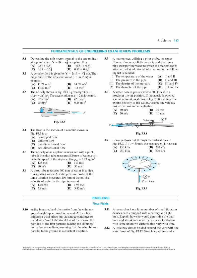
Problems 117
PROBLEMS
Flow Fields
3.10 A fire is started and the smoke from the chimneygoes straight up; no wind is present. After a fewminutes a wind arises but the smoke continues torise slowly. Sketch the streakline of the smoke, thepathline of the first particles leaving the chimney,and a few streamlines, assuming that the wind blowsparallel to the ground in a constant direction.
3.11 A researcher has a large number of small flotationdevices each equipped with a battery and lightbulb. Explain how she would determine the path-lines and streaklines near the surface of a streamwith some unknown currents that vary with time.
3.12 A little boy chases his dad around the yard with thewater hose of Fig. P3.12. Sketch a pathline and a
FUNDAMENTALS OF ENGINEERING EXAM REVIEW PROBLEMS
3.1 Determine the unit vector normal to the streamlineat a point where V � 3 î 4 j in a plane flow.(A) 0.6 î � 0.8 j (B) 0.6 î � 0.8 j(C) 0.8 î 0.6 j (D) 0.8 î � 0.6 j
3.2 A velocity field is given by V � 2xy î y2 j m/s. Themagnitude of the acceleration at (1 m, 2 m) isnearest:(A) 11.21 m/s2 (B) 14.69 m/s2
(C) 17.89 m/s2 (D) 1.2 m/s2
3.3 The velocity shown in Fig. P3.3 is given by V(x) �10/(4 x)2 m/s.The acceleration at x � 2 m is nearest:(A) 52.5 m/s2 (B) 42.5 m/s2
(C) 25 m/s2 (D) 6.25 m/s2
Fig. P3.3
3.4 The flow in the section of a conduit shown inFig. P3.3 is a:(A) developed flow(B) uniform flow(C) one-dimensional flow(D) two-dimensional flow
3.5 The velocity of an airplane is measured with a pitottube. If the pitot tube measures 800 mm of water, esti-mate the speed of the airplane. Use rair � 1.23 kg/m3.(A) 125 m/s (B) 113 m/s(C) 80 m/s (D) 36 m/s
3.6 A pitot tube measures 600 mm of water in a pipetransporting water. A static pressure probe at thesame location measures 200 mm of water. Thevelocity of water in the pipe is nearest:(A) 1.10 m/s (B) 1.98 m/s(C) 2.8 m/s (D) 3.43 m/s
V(x)x
3.7 A manometer, utilizing a pitot probe, measures10 mm of mercury. If the velocity is desired in apipe transporting water to which the manometer isattached, what additional information in the follow-ing list is needed?
I. The temperature of the water (A) I and IIII. The pressure in the pipe (B) II and III
III. The density of the mercury (C) III and IVIV. The diameter of the pipe (D) III and IV
3.8 A water hose is pressurized to 800 kPa with anozzle in the off position. If the nozzle is openeda small amount, as shown in Fig. P3.8, estimate theexiting velocity of the water. Assume the velocityinside the hose to be negligible.(A) 40 m/s (B) 30 m/s(C) 20 m/s (D) 10 m/s
Fig. P3.8
3.9 Benzene flows out through the disks shown inFig. P3.9. If V2 � 30 m/s, the pressure p1, is nearest:(A) 150 kPa (B) 200 kPa(C) 250 kPa (D) 300 kPa
Fig. P3.9
V1 = 15 m/s
p1
V2
r
pValve
V
Copyright 2010 Cengage Learning. All Rights Reserved. May not be copied, scanned, or duplicated, in whole or in part. Due to electronic rights, some third party content may be suppressed from the eBook and/or eChapter(s). Editorial review has deemed that any suppressed content does not materially affect the overall learning experience. Cengage Learning reserves the right to remove additional content at any time if subsequent rights restrictions require it.
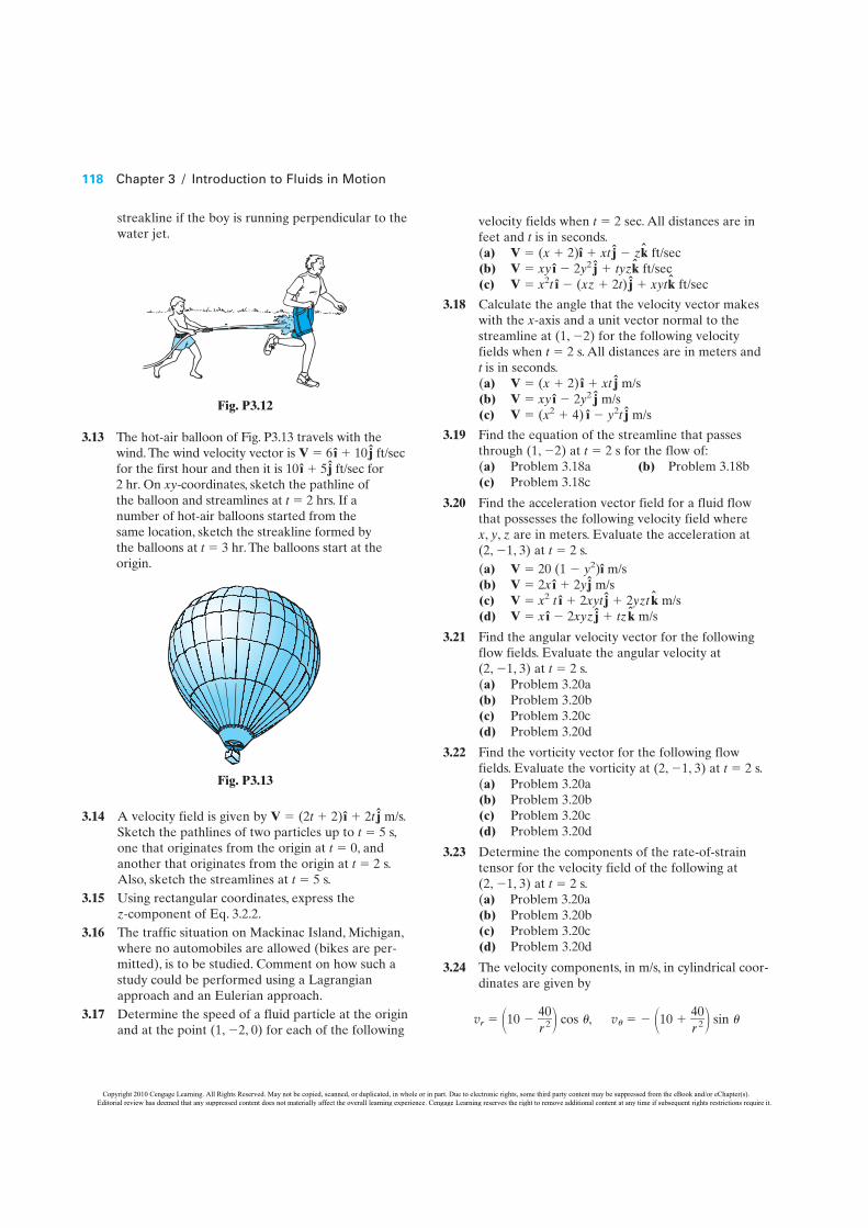
118 Chapter 3 / Introduction to Fluids in Motion
streakline if the boy is running perpendicular to thewater jet.
Fig. P3.12
3.13 The hot-air balloon of Fig. P3.13 travels with thewind. The wind velocity vector is V � 6 î � 10 j ft/secfor the first hour and then it is 10 î � 5 j ft/sec for2 hr. On xy-coordinates, sketch the pathline ofthe balloon and streamlines at t � 2 hrs. If anumber of hot-air balloons started from thesame location, sketch the streakline formed bythe balloons at t � 3 hr. The balloons start at theorigin.
Fig. P3.13
3.14 A velocity field is given by V � (2t � 2)î � 2t j m/s.Sketch the pathlines of two particles up to t � 5 s,one that originates from the origin at t � 0, andanother that originates from the origin at t � 2 s.Also, sketch the streamlines at t � 5 s.
3.15 Using rectangular coordinates, express the z-component of Eq. 3.2.2.
3.16 The traffic situation on Mackinac Island, Michigan,where no automobiles are allowed (bikes are per-mitted), is to be studied. Comment on how such astudy could be performed using a Lagrangianapproach and an Eulerian approach.
3.17 Determine the speed of a fluid particle at the originand at the point (1, 2, 0) for each of the following
velocity fields when t � 2 sec. All distances are infeet and t is in seconds.(a) V � (x � 2)î � xt j zk ft/sec(b) V � xy î 2y2 j � tyzk ft/sec(c) V � x2t î (xz � 2t) j � xytk ft/sec
3.18 Calculate the angle that the velocity vector makeswith the x-axis and a unit vector normal to thestreamline at (1, 2) for the following velocityfields when t � 2 s. All distances are in meters andt is in seconds.(a) V � (x � 2) î � xt j m/s(b) V � xy î 2y2 j m/s(c) V � (x2 � 4) î y2t j m/s
3.19 Find the equation of the streamline that passesthrough (1, 2) at t � 2 s for the flow of:(a) Problem 3.18a (b) Problem 3.18b(c) Problem 3.18c
3.20 Find the acceleration vector field for a fluid flowthat possesses the following velocity field where x, y, z are in meters. Evaluate the acceleration at (2, 1, 3) at t � 2 s.(a) V � 20 (1 y2)î m/s(b) V � 2x î � 2y j m/s(c) V � x2 t î � 2xyt j � 2yzt k m/s(d) V � x î 2xyz j � tzk m/s
3.21 Find the angular velocity vector for the followingflow fields. Evaluate the angular velocity at (2, 1, 3) at t � 2 s.(a) Problem 3.20a(b) Problem 3.20b(c) Problem 3.20c(d) Problem 3.20d
3.22 Find the vorticity vector for the following flowfields. Evaluate the vorticity at (2, 1, 3) at t � 2 s.(a) Problem 3.20a(b) Problem 3.20b(c) Problem 3.20c(d) Problem 3.20d
3.23 Determine the components of the rate-of-straintensor for the velocity field of the following at (2, 1, 3) at t � 2 s.(a) Problem 3.20a(b) Problem 3.20b(c) Problem 3.20c(d) Problem 3.20d
3.24 The velocity components, in m/s, in cylindrical coor-dinates are given by
vr � �10 �4r02�� cos u, vu � �10 � �
4r02�� sin u
Copyright 2010 Cengage Learning. All Rights Reserved. May not be copied, scanned, or duplicated, in whole or in part. Due to electronic rights, some third party content may be suppressed from the eBook and/or eChapter(s). Editorial review has deemed that any suppressed content does not materially affect the overall learning experience. Cengage Learning reserves the right to remove additional content at any time if subsequent rights restrictions require it.

Problems 119
(a) Calculate the acceleration of a fluid particleoccupying the point (4 m, 180°).
(b) Calculate the vorticity component at (4 m, 180°).
3.25 The velocity components, in m/s, in spherical coor-dinates are given by
vr � �10 �8r03�� cos u, vu � �10 � �
8r03�� sin u
(a) Calculate the acceleration of a fluid particleoccupying the point (4 m, 180°).
(b) Calculate the vorticity component at (4 m, 180°).
3.26 An unsteady flow occurs between parallel plates suchthat u � u(y, t), v � 0, and „ � 0. Write an expressionfor the acceleration. What is the acceleration if theflow is steady, that is, u � u(y), v � 0, and „ � 0?
3.27 Consider a symmetrical steady flow in a pipe with theaxial and radial velocity components designated u(r, x)and v(r, x), respectively.Write the equations for thetwo acceleration components ar and ax. Use equationsfrom Table 3.1. See Fig. P3.27 for the coordinates.
Fig. P3.27
3.28 The velocity in the 2-cm-diameter pipe of Fig. P3.28has only one nonzero velocity component given byu(r, t) � 2(1 r2/r2
0) (1 et/10) m/s, where r0 is theradius of the pipe and t is in seconds. Calculate themaximum velocity and the maximum acceleration:(a) Along the centerline of the pipe(b) Along a streamline at r � 0.5 cm(c) Along a streamline just next to the pipe wall[Hint: Let vz � u(r, t), vr � 0, and v� � 0 in theappropriate equations in Table 3.1.]
Fig. P3.28
u(r ,t)
(a)
r
x
υu
(a)
r
x
3.29 The temperature changes periodically in a flowaccording to T(y, t) � 20 (1 y2) cos pt/100°C. Ifthe velocity is given by u � 2 (1 y2) m/s, deter-mine the rate of change of the temperature of afluid particle located at y � 0 if t � 20 s.
3.30 The density of air in the atmosphere varies accord-ing to r(z) � 1.23e104z kg/m3. Air flowing overthe mountain of Fig. P3.30 has the velocity vectorV � 20 î � 10 k m/s at a location of interest wherez � 3000 m. Find the rate at which a particle’s den-sity is changing at that location.
Fig. P3.30
3.31 The density variation with elevation is given byr(z) � 1000 (1 z/4) kg/m3. At a location whereV � 10 î � 10k m/s, find Dr/Dt.
3.32 Salt is slowly added to water in a pipe so that�r/�x � 0.01 kg/m4. Determine Dr/Dt if thevelocity is uniform at 4 m/s.
3.33 Express the substantial derivative in terms of thegradient � and the velocity vector V. Recall fromcalculus that in rectangular coordinates
� � ��
�
x� î � �
�
�
y� j � �
�
�
z� k
3.34 We can write Eqs. 3.2.9 in a simplified vector form.The gradient is a vector operator expressed in rec-tangular coordinates as � � �
�
�
x� î � �
�
�
y� j � �
�
�
z� k.
Write the dot product of the velocity vector V and thegradient � and then write Eqs. 3.2.9 as one vector equa-tion expressing the acceleration a as the sum of the localacceleration and the convective acceleration.
3.35 For the flow shown in Fig. P3.35, relative to a fixedreference frame, find the acceleration of a fluid par-ticle at:(a) Point A(b) Point BThe water at B makes an angle of 30° withrespect to the ground and the sprinkler arm ishorizontal.
3000 m
V
Copyright 2010 Cengage Learning. All Rights Reserved. May not be copied, scanned, or duplicated, in whole or in part. Due to electronic rights, some third party content may be suppressed from the eBook and/or eChapter(s). Editorial review has deemed that any suppressed content does not materially affect the overall learning experience. Cengage Learning reserves the right to remove additional content at any time if subsequent rights restrictions require it.

120 Chapter 3 / Introduction to Fluids in Motion
Classification of Fluid Flows
3.37 Consider each of the following flows and statewhether it could be approximated as a one-,two-, or three-dimensional flow or as auniform flow:(a) Flow from a vertical pipe striking a horizontal
wall(b) Flow in the waves of the ocean near a beach(c) Flow near the entrance of a pipe(d) Flow around a rocket with a blunt nose(e) Flow around an automobile(f) Flow in an irrigation channel(g) Flow through an artery(h) Flow through a vein
3.38 Which of the flows in Problem 3.37 could beassumed to be a steady flow? Which must be mod-eled as an unsteady flow?
3.39 Which flow in Problem 3.37 could best be modeledas a plane flow?
3.40 Select the flows in Problem 3.37 that would possessa stagnation point. Sketch each of the selectedflows indicating the location of the stagnationpoint.
3.41 Which of the flows in Problem 3.37 could be modeled as a developed flow?
3.42 State whether each of the flows in Problem 3.37could be considered as primarily an inviscid flow ora viscous flow.
3.43 Select the flows in Problem 3.37 that are externalflows. Does each of the external flows possess astagnation point?
3.44 Sketch the flow around a razor blade positionedparallel to the flow showing the boundary layers.
3.45 The 32°C water exiting the 1.5-cm-diameter faucetof Fig. P3.45 has an average velocity of 2 m/s.Would you expect the flow to be laminar orturbulent?
Fig. P3.45
3.46 The Red Cedar River flows placidly throughMichigan State University’s campus. In a certainsection the depth is 2.5 ft and the average velocityis 0.6 fps. Is the flow laminar or turbulent?
3.47 Air at 40°C flows in a rectangular 30 cm � 6 cmheating duct at an average velocity of 4 m/s. Is theflow laminar or turbulent?
3.48 The sphere of diameter D of Fig. P3.48 is travelingwith a velocity V of 1.2 m/s in 20°C atmospheric air.If Re � VD/n is less than 4 � 104, the boundarylayer around the front of the sphere is completelylaminar. Determine if the boundary layer is com-pletely laminar on a sphere of diameter:(a) 1 cm (b) 1 m
Fig. P3.48
VBoundary
layer
Fig. P3.35
20 rad/s
A 12 ft/sec
4.5 ft 4.5 ft
B
60 ft/sec
3.36 A river is flowing due south at 5 m/s at a latitude of45°. Calculate the acceleration of a particle floatingwith the river relative to a fixed reference frame.The radius of the Earth is 6400 km.
Copyright 2010 Cengage Learning. All Rights Reserved. May not be copied, scanned, or duplicated, in whole or in part. Due to electronic rights, some third party content may be suppressed from the eBook and/or eChapter(s). Editorial review has deemed that any suppressed content does not materially affect the overall learning experience. Cengage Learning reserves the right to remove additional content at any time if subsequent rights restrictions require it.

Problems 121
Bernoulli’s Equation
3.54 A pitot tube is used to measure the velocity of asmall aircraft flying at 3000 ft. Calculate its velocityif the pitot tube measures:(a) 0.3 psi (b) 0.9 psi (c) 0.09 psi
3.55 Approximate the force acting on the 15-cm-diame-ter headlight shown in Fig. P3.55 of an automobiletraveling at 120 kph.
Fig. P3.55
3.56 A vacuum cleaner is capable of creating a vacuum of2 kPa just inside the hose of Fig. P3.56.What maxi-mum average velocity would be expected in the hose?
Fig. P3.56
V
15 cm
V
3.57 The inviscid, incompressible flow in the vicinity ofa stagnation point (Fig. P3.57) is approximated byu � 10x, v � 10y. If the pressure at the origin isp0, find an expression for the pressure neglectinggravity effects:(a) Along the negative x-axis(b) Along the positive y-axis
Fig. P3.57
y
υ
xu
3.49 The airfoil on a commercial airliner is approxi-mated as a flat plate sketched in Fig. P3.49. Howlong would you expect the laminar portion of theboundary layer to be if it is flying:
(a) At an altitude of 10 000 m and a speed of 900 km/h?
(b) At an altitude of 30,000 ft and a speed of 600 mph?
Fig. P3.49
3.50 A leaf keeps cool by transpiration, a process in whichwater flows from the leaf to the atmosphere. Anexperimenter wonders if the boundary layer on a leafinfluences the transpiration, so an “experimental” leaf
V
xT
is set up in the laboratory and air is blown parallel toit at 6 m/s. Comment as to whether the boundarylayer is expected to be laminar or turbulent.
3.51 For the following situations state whether a com-pressible flow is required or if the flow can beapproximated with an incompressible flow:
(a) An aircraft flying at 100 m/s at an elevation of8000 m
(b) A golf ball traveling at 240 ft/sec
(c) Flow around an object being studied in a high-temperature wind tunnel if the temperature is100°C and the air velocity is 100 m/s
3.52 Write out Eq. 3.3.2 using Eq. 3.2.11. For a steady,plane flow what relationship must exist for an incom-pressible flow in which the density is allowed to vary?
3.53 If r � r0 (1 � cz) models the density variation ina channel (there is heavy salt water at the bottomand fresh water at the top) in which u(y, z) is theonly velocity component, is the flow incompressible?
Copyright 2010 Cengage Learning. All Rights Reserved. May not be copied, scanned, or duplicated, in whole or in part. Due to electronic rights, some third party content may be suppressed from the eBook and/or eChapter(s). Editorial review has deemed that any suppressed content does not materially affect the overall learning experience. Cengage Learning reserves the right to remove additional content at any time if subsequent rights restrictions require it.

122 Chapter 3 / Introduction to Fluids in Motion
3.58 The inviscid, incompressible flow field exterior tothe cylinder shown in Fig. P3.58 is given by
vr � U��1 �r
r2
2c�� cos u, vu � U��1 � �
r
r2
2c�� sin u
If the pressure at r � � is zero (i.e., p� � 0), find anexpression for the pressure neglecting gravityeffects:(a) Along the negative x-axis(b) At the stagnation point(c) On the surface of the cylinder(d) On the surface of the cylinder at � � 90°
Fig. P3.58
3.59 The inviscid, incompressible flow field exterior to a sphere (see Fig. P3.58) is given by
vr � U��1 �r
r3
3c�� cos u, vu � U��1 � �
r
r3
3c�� sin u
If the pressure at r � � is zero, find an expressionfor the pressure neglecting gravity effects:(a) Along the negative x-axis(b) At the stagnation point(c) On the surface of the sphere(d) On the surface of the sphere at u � 90°
3.60 The velocity along the negative x-axis in theinviscid, incompressible flow field exterior tothe body shown in Fig. P3.60 is given by u(x) � U� � q/2px. If the pressure at x � �is zero, find an expression for the pressureneglecting gravity effects:(a) Along the negative x-axis if U� � 10 m/s and
q � 20p m2/s(b) At the stagnation point if U� � 10 m/s and
q � 20p m2/s
rc
r
r
θ
θ
υ
υ
U∞
(c) Along the negative x-axis if U� � 30 ft/secand q � 60p ft2/sec
(d) At the stagnation point if U� � 30 ft/sec andq � 60p ft2/sec
Fig. P3.60
3.61 The incompressible flow of water through the shortcontraction of Fig. 3.19a is assumed to be inviscid.If a pressure drop of 20 kPa is measured, estimatethe velocity at the wall at section 2 just downstreamof the contraction. (Actually, a boundary layerwould develop, and the velocity calculated at thewall would be the velocity at the edge of theboundary layer; see the inset of Fig. 3.10.)
3.62 Air flows from a relatively large plenum in a fur-nace out a relatively small rectangular duct. If thepressure in the plenum measures 60 Pa and in theduct 10.2 Pa, estimate the velocity of the 40°C air inthe duct.
3.63 A short contraction is followed by an expansion,as shown in Fig. P3.63.The manometer is used todetermine the velocity of the fluid providing theviscous effects are negligible. If water is flowingsteadily, determine the velocity V1 if H � 12 cm.Losses through the contraction are negligible.
Fig. P3.63
Water
DatumHgH
V2V1
x
Water
U∞
Copyright 2010 Cengage Learning. All Rights Reserved. May not be copied, scanned, or duplicated, in whole or in part. Due to electronic rights, some third party content may be suppressed from the eBook and/or eChapter(s). Editorial review has deemed that any suppressed content does not materially affect the overall learning experience. Cengage Learning reserves the right to remove additional content at any time if subsequent rights restrictions require it.

Problems 123
3.64 What is the velocity of the water in the pipe if themanometer shown in Fig. P3.64 reads:(a) 4 cm?(b) 10 cm?(c) 2 in.?(d) 4 in.?
Fig. P3.64
3.65 Air at 120 kPa absolute and 30°C flows verticallyupward in a pipe, as shown in Fig. P3.65. If thewater manometer deflection H � 5 cm, determinethe velocity in the smaller pipe. Assume the air tobe incompressible.
Fig. P3.65
3.66 A manometer, positioned inside a cylinder asshown in Fig. P3.66, reads 4 cm of water.Estimate U� assuming an inviscid flow. Refer tothe velocity field in Problem 3.58.
V2
Air
Datum
1.5 m
H
Water
1
V1
HgV
H Fig. P3.66
3.67 A manometer, positioned as shown in Figure P3.66inside a sphere, reads 4 cm of water. Estimate U�
assuming an inviscid flow. Refer to the velocityfield in Problem 3.59.
3.68 For the flow shown in Fig. P3.68, estimate the pres-sure p1 and velocity V1 if V2 � 20 m/s and:(a) H � 1 cm(b) H � 5 cm(c) H � 10 cm
Water
Atmosphere20°C air
U∞H
H
V1
p1
Water
Hg
3.69 Water at 15°C flows steadily through the contractionshown in Fig. P3.69 such that V2 � 4V1. If the gagereading is maintained at 120 kPa, determine the max-imum velocity V1 possible before cavitation occurs.
Fig. P3.68
V1
Water
120 kPa
V2 V1
Fig. P3.69
Copyright 2010 Cengage Learning. All Rights Reserved. May not be copied, scanned, or duplicated, in whole or in part. Due to electronic rights, some third party content may be suppressed from the eBook and/or eChapter(s). Editorial review has deemed that any suppressed content does not materially affect the overall learning experience. Cengage Learning reserves the right to remove additional content at any time if subsequent rights restrictions require it.

124 Chapter 3 / Introduction to Fluids in Motion
3.70 In the pipe contraction shown in Fig. P3.70, waterflows steadily with a velocity of V1 � 0.5 m/s andV2 � 1.125 m/s. Two piezometer tubes are attachedto the pipe at sections 1 and 2. Determine the heightH. Neglect any losses through the contraction.
Fig. P3.70
3.71 Air at 20°C is drawn into the hose of a vacuumcleaner through a head that is relatively free ofobstructions (the flow can be assumed to be invis-cid). Estimate the velocity in the hose if the vacu-um in the hose measures:(a) 2 cm of water (b) 8 cm of water(c) 1 in. of water (d) 4 in. of water
3.72 A wind tunnel is designed to draw in air from theatmosphere and produce a velocity of 100 m/s inthe test section. The fan is located downstream ofthe test section. What pressure is to be expected inthe test section if the atmospheric temperature andpressure are:(a) 20°C, 90 kPa? (b) 0°C, 95 kPa?(c) 20°C, 92 kPa? (d) 40°C, 100 kPa?
3.73 The pump shown in Fig. P3.73 creates a flow suchthat V � 14 m/s. Predict the pressure at the gageshown assuming an inviscid flow in the entranceand a uniform flow at the gage. Use a streamlinestarting at:(a) Point A (b) Point B
Fig. P3.73
V
Water
AP
p
B
4 m
Water
25 cm
V1 V2
H
3.74 A fireman reduces the exit area on a nozzle so thatthe velocity inside the hose is quite small relative tothe exiting velocity. What is the maximum exitingvelocity and what is the maximum height the watercan reach if the pressure inside the hose is:(a) 700 kPa? (b) 1400 kPa?(c) 100 psi? (d) 200 psi?
3.75 The velocity downstream of a sluice gate is assumedto be uniform (Fig. P3.75). Express V in terms of Hand h for this inviscid flow. Use a streamline:(a) Along the top downstream(b) Along the bottom downstream
Fig. P3.75
3.76 To what maximum velocity can water be acceleratedbefore it reaches the turbine blades of a hydro-turbine if it enters with relatively low velocity at:(a) 600 kPa? (b) 300 kPa?(c) 80 psi? (d) 40 psi?
3.77 Water exists in a city’s water system at a pressureof 500 kPa at a particular location. The water pipemust traverse over a hill. How high could the hillbe, above that location, for the system to possiblysupply water to the other side of the hill?
3.78 Fluid flows between the radial disks shown inFig. P3.78. Estimate the pressure in the 2-cm-diameter pipe if the fluid exits to the atmosphere.Neglect viscous effects. The fluid is:(a) Water (b) Benzene(c) Gasoline (d) Air
Fig. P3.78
r
V1 = 10 m/s
V2 = 20 m/s
2 cm
H
Sluice gate
h
Water
V1 = 0~
Copyright 2010 Cengage Learning. All Rights Reserved. May not be copied, scanned, or duplicated, in whole or in part. Due to electronic rights, some third party content may be suppressed from the eBook and/or eChapter(s). Editorial review has deemed that any suppressed content does not materially affect the overall learning experience. Cengage Learning reserves the right to remove additional content at any time if subsequent rights restrictions require it.

Problems 125
3.79 Estimate the pressure at r � 10 cm if the velocitythere is 30 m/s in Problem 3.78d.
3.80 It is proposed that air blown through a tubeattached to a metal disk be used to pick upenvelopes, as shown in Fig. P3.80. Would such asetup actually pick up an envelope? Explain.Assume an inviscid flow with the air slowing downas it moves radially outward.
Fig. P3.80
3.81 From which of the following objects would youexpect the flow to separate and form a substantialseparated region?(a) A golf ball(b) A telephone wire(c) A wind machine blade(d) A 2-mm-diameter wire in a low-speed wind
tunnel(e) An automobile(f) An aircraft(Note: Separation occurs whenever the Reynoldsnumber exceeds a value around 20 over a bluntobject.)
3.82 Explain, with the use of a sketch, why a burr on thedownstream side of a piezometer opening in a pipe(see Fig. 3.18a) will result in a reading of the pres-sure that is too high.
Envelope Metal disc
Tube
V
3.83 An incompressible, inviscid flow of water enters abend with a uniform velocity of V1 � 10 m/s(Fig. P3.83). Estimate the pressure difference betweenpoints A and B if the average radius of curvature atthe bend is 5 cm. Sketch an anticipated velocity pro-file along AB.Assume that pA p1 and pB � p1.
Fig. P3.83
3.84 Viscosity causes a fluid to stick to a surface. If thefluid in Problem 3.83 sticks to the surface, explainwhy, in a viscous flow, a secondary flow is caused bythe bend. Sketch such a flow on a circular crosssection at section 2.
3.85 In Fig. P3.85, assuming an inviscid flow, insert oneof these signs between the pressures: �, , � .
pA pB
pC pD
pB pD
A
V1
2 cm
B
1
2
A
B D
C
Fig. P3.85
Copyright 2010 Cengage Learning. All Rights Reserved. May not be copied, scanned, or duplicated, in whole or in part. Due to electronic rights, some third party content may be suppressed from the eBook and/or eChapter(s). Editorial review has deemed that any suppressed content does not materially affect the overall learning experience. Cengage Learning reserves the right to remove additional content at any time if subsequent rights restrictions require it.