
Introduction to Elastic Wave Propagation - iMechanicaimechanica.org/files/awave.pdfIntroduction vi...
385
Introduction to Elastic Wave Propagation A. Bedford & D. S. Drumheller
-
Upload
truongkhuong -
Category
Documents
-
view
219 -
download
3
Transcript of Introduction to Elastic Wave Propagation - iMechanicaimechanica.org/files/awave.pdfIntroduction vi...
Introduction to
Elastic Wave Propagation
A. Bedford & D. S. Drumheller

This document contains the complete text of the book published in 1994 byJohn Wiley & Sons Ltd., Chichester, England. It has been edited and asection on the finite element method added. Copyright by A. Bedford andD. S. Drumheller.
i
Contents
Introduction vi
Nomenclature viii
1 Linear Elasticity 11.1 Index Notation . . . . . . . . . . . . . . . . . . . . . . . . . . . . 1
Cartesian coordinates and vectors . . . . . . . . . . . . . . . . 1Dot and cross products . . . . . . . . . . . . . . . . . . . . . . 3Gradient, divergence, and curl . . . . . . . . . . . . . . . . . . 4Gauss theorem . . . . . . . . . . . . . . . . . . . . . . . . . . . 4
1.2 Motion . . . . . . . . . . . . . . . . . . . . . . . . . . . . . . . . . 8The motion and inverse motion . . . . . . . . . . . . . . . . . 9Velocity and acceleration . . . . . . . . . . . . . . . . . . . . . 9
1.3 Deformation . . . . . . . . . . . . . . . . . . . . . . . . . . . . . . 14Strain tensor . . . . . . . . . . . . . . . . . . . . . . . . . . . . 14Longitudinal strain . . . . . . . . . . . . . . . . . . . . . . . . 15Shear strain . . . . . . . . . . . . . . . . . . . . . . . . . . . . 17Changes in volume and density . . . . . . . . . . . . . . . . . 19
1.4 Stress . . . . . . . . . . . . . . . . . . . . . . . . . . . . . . . . . 24Traction . . . . . . . . . . . . . . . . . . . . . . . . . . . . . . 24Stress tensor . . . . . . . . . . . . . . . . . . . . . . . . . . . . 25Tetrahedron argument . . . . . . . . . . . . . . . . . . . . . . 26
1.5 Stress-Strain Relations . . . . . . . . . . . . . . . . . . . . . . . . 32Linear elastic materials . . . . . . . . . . . . . . . . . . . . . . 32Isotropic linear elastic materials . . . . . . . . . . . . . . . . . 32
1.6 Balance and Conservation Equations . . . . . . . . . . . . . . . . 37Transport theorem . . . . . . . . . . . . . . . . . . . . . . . . 37Conservation of mass . . . . . . . . . . . . . . . . . . . . . . . 38Balance of linear momentum . . . . . . . . . . . . . . . . . . . 39
ii

Balance of angular momentum . . . . . . . . . . . . . . . . . . 401.7 Equations of Motion . . . . . . . . . . . . . . . . . . . . . . . . . 42
Displacement equations of motion . . . . . . . . . . . . . . . . 42Helmholtz decomposition . . . . . . . . . . . . . . . . . . . . . 43Acoustic medium . . . . . . . . . . . . . . . . . . . . . . . . . 44
1.8 Summary . . . . . . . . . . . . . . . . . . . . . . . . . . . . . . . 46Displacement equations of motion . . . . . . . . . . . . . . . . 46Helmholtz decomposition . . . . . . . . . . . . . . . . . . . . . 46Strain tensor and density . . . . . . . . . . . . . . . . . . . . . 47Stress-strain relation . . . . . . . . . . . . . . . . . . . . . . . 47Traction . . . . . . . . . . . . . . . . . . . . . . . . . . . . . . 47
2 One-Dimensional Waves 482.1 One-Dimensional Wave Equation . . . . . . . . . . . . . . . . . . 482.2 One-Dimensional Motions of an Elastic Material . . . . . . . . . 54
Compressional waves . . . . . . . . . . . . . . . . . . . . . . . 54Shear waves . . . . . . . . . . . . . . . . . . . . . . . . . . . . 57
2.3 Motion of a String . . . . . . . . . . . . . . . . . . . . . . . . . . 60Equation of motion . . . . . . . . . . . . . . . . . . . . . . . . 60Boundary conditions . . . . . . . . . . . . . . . . . . . . . . . 61
2.4 One-Dimensional Solutions . . . . . . . . . . . . . . . . . . . . . 63Initial-value problem . . . . . . . . . . . . . . . . . . . . . . . 63Initial-boundary value problems . . . . . . . . . . . . . . . . . 66Reflection and transmission at an interface . . . . . . . . . . . 70
2.5 The Finite Element Method . . . . . . . . . . . . . . . . . . . . . 78One-dimensional waves in a layer . . . . . . . . . . . . . . . . 78Basis functions . . . . . . . . . . . . . . . . . . . . . . . . . . 81The finite element solution . . . . . . . . . . . . . . . . . . . . 81Evaluation of the mass and stiffness matrices . . . . . . . . . . 85Numerical integration with respect to time . . . . . . . . . . . 88Example . . . . . . . . . . . . . . . . . . . . . . . . . . . . . . 89
2.6 Method of Characteristics . . . . . . . . . . . . . . . . . . . . . . 93Initial-value problem . . . . . . . . . . . . . . . . . . . . . . . 94Initial-boundary value problem . . . . . . . . . . . . . . . . . 95
2.7 Waves in Layered Media . . . . . . . . . . . . . . . . . . . . . . . 99First algorithm . . . . . . . . . . . . . . . . . . . . . . . . . . 100Second algorithm . . . . . . . . . . . . . . . . . . . . . . . . . 101Examples . . . . . . . . . . . . . . . . . . . . . . . . . . . . . 102
iii

3 Steady-State Waves 1103.1 Steady-State One-Dimensional Waves . . . . . . . . . . . . . . . 1103.2 Steady-State Two-Dimensional Waves . . . . . . . . . . . . . . . 118
Plane waves propagating in the x1-x3 plane . . . . . . . . . . 119Plane waves propagating in the x1 direction and attenuating
in the x3 direction . . . . . . . . . . . . . . . . . . . . . . 1233.3 Reflection at a Plane Boundary . . . . . . . . . . . . . . . . . . . 126
Incident compressional wave . . . . . . . . . . . . . . . . . . . 126Incident shear wave . . . . . . . . . . . . . . . . . . . . . . . . 132
3.4 Rayleigh Waves . . . . . . . . . . . . . . . . . . . . . . . . . . . . 1403.5 Steady-State Waves in a Layer . . . . . . . . . . . . . . . . . . . 143
Acoustic waves in a channel . . . . . . . . . . . . . . . . . . . 143Waves in an elastic layer . . . . . . . . . . . . . . . . . . . . . 147Elementary theory of waves in a layer . . . . . . . . . . . . . . 151
3.6 Steady-State Waves in Layered Media . . . . . . . . . . . . . . . 154Special cases . . . . . . . . . . . . . . . . . . . . . . . . . . . . 156Pass and stop bands . . . . . . . . . . . . . . . . . . . . . . . 157
4 Transient Waves 1594.1 Laplace Transform . . . . . . . . . . . . . . . . . . . . . . . . . . 1594.2 Fourier Transform . . . . . . . . . . . . . . . . . . . . . . . . . . 164
Example . . . . . . . . . . . . . . . . . . . . . . . . . . . . . . 164Fourier superposition and impulse response . . . . . . . . . . . 167
4.3 Discrete Fourier Transform . . . . . . . . . . . . . . . . . . . . . 1724.4 Transient Waves in Dispersive Media . . . . . . . . . . . . . . . . 182
Group velocity . . . . . . . . . . . . . . . . . . . . . . . . . . . 182Transient waves in layered media . . . . . . . . . . . . . . . . 185
4.5 Cagniard-de Hoop Method . . . . . . . . . . . . . . . . . . . . . . 196
5 Nonlinear Wave Propagation 2125.1 One-Dimensional Nonlinear Elasticity . . . . . . . . . . . . . . . 213
Motion . . . . . . . . . . . . . . . . . . . . . . . . . . . . . . . 213Deformation gradient and longitudinal strain . . . . . . . . . . 213Conservation of mass . . . . . . . . . . . . . . . . . . . . . . . 214Balance of linear momentum . . . . . . . . . . . . . . . . . . . 215Stress-strain relation . . . . . . . . . . . . . . . . . . . . . . . 216Summary . . . . . . . . . . . . . . . . . . . . . . . . . . . . . . 216
5.2 Hyperbolic Systems and Characteristics . . . . . . . . . . . . . . 217Characteristics . . . . . . . . . . . . . . . . . . . . . . . . . . . 218
iv

Interior equation and hyperbolic equations . . . . . . . . . . . 219Examples . . . . . . . . . . . . . . . . . . . . . . . . . . . . . 220Weak waves . . . . . . . . . . . . . . . . . . . . . . . . . . . . 226
5.3 Singular Surface Theory . . . . . . . . . . . . . . . . . . . . . . . 233Kinematic compatibility condition . . . . . . . . . . . . . . . . 233Acceleration waves . . . . . . . . . . . . . . . . . . . . . . . . 235Shock waves . . . . . . . . . . . . . . . . . . . . . . . . . . . . 237
5.4 Loading and Release Waves . . . . . . . . . . . . . . . . . . . . . 242
Bibliography 252
Index 253
Solutions to the Exercises 258
A Complex Analysis 353A.1 Complex Variables . . . . . . . . . . . . . . . . . . . . . . . . . . 353A.2 Contour Integration . . . . . . . . . . . . . . . . . . . . . . . . . 356A.3 Multiple-Valued Functions . . . . . . . . . . . . . . . . . . . . . . 365
B Tables of Material Properties 370
v

Introduction
Earthquakes are detected and studied by measuring the waves they create.Waves are transmitted through the Earth to detect oil and gas deposits andto study the Earth’s geological structure. Properties of materials are deter-mined by measuring the behavior of waves transmitted through them. In recentyears, elastic waves transmitted through the human body have been used formedical diagnosis and therapy. Many students and professionals in the variousbranches of engineering and in physics, geology, mathematics, and the life sci-ences encounter problems requiring an understanding of elastic waves. In thisbook we present the basic concepts and methods of the theory of wave propa-gation in elastic materials in a form suitable for a one-semester course at theadvanced undergraduate or graduate level, for self-study, or as a supplement incourses that include material on elastic waves. Because persons with such dif-ferent backgrounds are interested in elastic waves, we provide a more completediscussion of the theory of elasticity than is usually found in a book of this type,and also an appendix on the theory of functions of a complex variable. Whilepersons who are well versed in mechanics and partial differential equations willhave a deeper appreciation for some of the topics we discuss, the basic materialin Chapters 1-3 requires no preparation beyond a typical undergraduate calculussequence.
Chapter 1 covers linear elasticity through the displacement equations ofmotion. Chapter 2 introduces the one-dimensional wave equation and theD’Alembert solution. We show that one-dimensional motions of a linear elas-tic material are governed by the one-dimensional wave equation and discusscompressional and shear waves. To provide help in understanding and visual-izing elastic waves, we demonstrate that small lateral motions of a stretchedstring (such as a violin string) are governed by the one-dimensional wave equa-tion and show that the boundary conditions for a string are analogous to theboundary conditions for one-dimensional motions of an elastic material. Usingthe D’Alembert solution, we analyze several problems, including reflection and
vi

Introduction vii
transmission at a material interface. We define the characteristics of the one-dimensional wave equation and show how they can be used to obtain solutions.We apply characteristics to layered materials and describe simple numerical al-gorithms for solving one-dimensional problems in materials with multiple layers.
Chapter 3 is concerned with waves having harmonic (oscillatory) time de-pendence. We present the solution for reflection at a free boundary and discussRayleigh waves. To introduce the concepts of dispersion and propagation modes,we analyze the propagation of sound waves down a two-dimensional channel. Wethen discuss longitudinal waves in an elastic layer and waves in layered media.
Chapter 4 is devoted to transient waves. We introduce the Fourier andLaplace transforms and illustrate some of their properties by applying themto one-dimensional problems. We introduce the discrete Fourier transform andapply it to several examples using the FFT algorithm. We define the concept ofgroup velocity and use our analyses of layered media from Chapters 2 and 3 todiscuss and demonstrate the propagation of transient waves in dispersive media.
Chapter 5 discusses some topics in nonlinear wave propagation. Althoughfew applications involving nonlinear waves in solid materials can be analyzedadequately by assuming elastic behavior, we discuss and demonstrate some ofthe important concepts using an elastic material as an heuristic example. Afterpresenting the theory of nonlinear elasticity in one dimension, we discuss hyper-bolic systems of first-order equations and characteristics and derive the class ofexact solutions called simple waves. We introduce singular surface theory anddetermine the properties of acceleration waves and shock waves. The chapterconcludes with a discussion of the steady compressional waves and release wavesobserved in experimental studies of large-amplitude waves.

Nomenclature
Definitions of frequently-used symbols. The pages on which they first appearare shown in parentheses.
a, ak Acceleration (2).
b, bk Body force (28).
Bk Basis function (81)
c1 Phase velocity (146).
cp Plate velocity (151).
cg Group velocity (183).
c Slope of characteristic (221).Constant in Hugoniot relation (244).
C, Ckm Mass matrix (84).
d, dk Vector of nodal displacements (84).
ekmn Alternator (3).
Emn Lagrangian strain (15).
E Young’s modulus (34).
F, Fk Force (2).
f Frequency, Hz (112).
F Deformation gradient (214).
fF (ω) Fourier transform of f (164).
fL(s) Laplace transform of f (159).
viii

Nomenclature ix
fDFm Discrete Fourier transform of fm
(172).
f , fk Force vector (84).
H(t) Step function (76).
i, ik Unit direction vector (1).
i√−1 (113).
j Nondimensional time (100).
k Wave number (111).
K, Kkm Stiffness matrix (84).
m Nondimensional time (175).
n Unit vector to surface (4).
n Nondimensional position (100).
p Pressure (25).
r Magnitude of complex variable (354).
s Laplace transform variable (159).Constant in Hugoniot relation (244).
S Surface (4).
t Time (4).
t, tk Traction (24).
Tkm Stress tensor (26).
T Window length of FFT (172).Period (112).Normal stress (215).
u, uk Displacement vector (9).
u Dependent variable (48).Real part (354).
U Shock wave velocity (243).

Nomenclature x
v, vk Velocity (9).
v Velocity (93).Imaginary part (354).
V Volume (4).
x, xk Position (9).
X, Xk Reference position (9).
z Acoustic impedance (72).Complex variable (353).
α Compressional wave velocity (55).Phase velocity (111).
β Shear wave velocity (58).
γkm Shear strain (18).
δkm Kronecker delta (3).
Δ Time increment (100).
ε Longitudinal strain (15).Negative of the longitudinal strain(214).
ζ Characteristic coordinate (218).Steady-wave variable (243).
η D’Alembert variable (49).Characteristic coordinate (218).
θ Propagation direction (120).Phase of complex variable (354).
θc Critical propagation direction (135).
λ Lame constant (34).Wavelength (111).
μ Lame constant, shear modulus (34).
ν Poisson’s ratio (34).

Nomenclature xi
ξ D’Alembert variable (49).
ρ Density (20).
ρ0 Density in reference state (21).
σ Normal stress (25).
τ Shear stress (25).
φ Helmholtz scalar potential (43).
ψ, ψk Helmholtz vector potential (43).
ω Frequency, rad/s (110).
Chapter 1
Linear Elasticity
To analyze waves in elastic materials, we must derive the equa-tions governing the motions of such materials. In this chapter weshow how the motion and deformation of a material are describedand discuss the internal forces, or stresses, in the material. We defineelastic materials and present the relation between the stresses andthe deformation in a linear elastic material. Finally, we introducethe postulates of conservation of mass and balance of momentumand use them to obtain the equations of motion for a linear elasticmaterial.
1.1 Index Notation
Here we introduce a compact and convenient way to express the equations usedin elasticity.
Cartesian coordinates and vectors
Consider a cartesian coordinate system with coordinates x, y, z and unit vec-tors i, j,k (Fig. 1.1.a). We can express a vector v in terms of its cartesiancomponents as
v = vx i + vy j + vz k.
Let us make a simple change of notation, renaming the coordinates x1, x2, x3
and the unit vectors i1, i2, i3 (Fig. 1.1.b). The subscripts 1, 2, 3 are called indices.With this notation, we can express the vector v in terms of its components in
1

Chapter 1. Linear Elasticity 2
(a) (b)
��
x
y
z
i
j
k
v
��
x1
x2
x3
i1
i2
i3
v
�
�
���
������
�
�
���
������
Figure 1.1: A cartesian coordinate system and a vector v. (a) Traditionalnotation. (b) Index notation.
the compact form
v = v1 i1 + v2 i2 + v3 i3 =3∑
k=1
vk ik.
We can write the vector v in an even more compact way by using what is calledthe summation convention. Whenever an index appears twice in an expression,the expression is assumed to be summed over the range of the index . With thisconvention, we can write the vector v as
v = vk ik.
Because the index k appears twice in the expression on the right side of thisequation, the summation convention tells us that
v = vk ik = v1 i1 + v2 i2 + v3 i3.
In vector notation, Newton’s second law is
F = ma.
In index notation, we can write Newton’s second law as the three equations
F1 = ma1,
F2 = ma2,
F3 = ma3,
where F1, F2, F3 are the cartesian components of F and a1, a2, a3 are the carte-sian components of a. We can write these three equations in a compact way by

Chapter 1. Linear Elasticity 3
using another convention: Whenever an index appears once in each term of anequation, the equation is assumed to hold for each value in the range of thatindex. With this convention, we write Newton’s second law as
Fk = mak.
Because the index k appears once in each term, this equation holds for k = 1,k = 2, and k = 3.
Dot and cross products
The dot and cross products of two vectors are useful definitions from vectoranalysis. By expressing the vectors in index notation, we can write the dotproduct of two vectors u and v as
u · v = (ukik) · (vmim)
= ukvm(ik · im).
The dot product ik · im equals one when k = m and equals zero when k �= m.By introducing the Kronecker delta
δkm ={
1 when k = m,0 when k �= m,
we can write the dot product of the vectors u and v as
u · v = ukvmδkm.
We leave it as an exercise to show that
ukvmδkm = u1v1 + u2v2 + u3v3,
which is the familiar expression for the dot product of the two vectors in termsof their cartesian components.
We can write the cross product of two vectors u and v as
u × v = (ukik) × (vmim)
= ukvm(ik × im).
The values of the cross products of the unit vectors are
ik × im = ekmn in,
where the term ekmn, called the alternator, is defined by
ekmn =
⎧⎨⎩
0 when any two of the indices k,m, n are equal,1 when kmn = 123 or 312 or 231,
−1 otherwise.
Thus we can write the cross product of the vectors u and v as
u × v = ukvmekmn in.
Chapter 1. Linear Elasticity 4
Gradient, divergence, and curl
A scalar field is a function that assigns a scalar value to each point of a region inspace during some interval of time. The expression for the gradient of a scalarfield φ = φ(x1, x2, x3, t) in terms of cartesian coordinates is
∇φ =∂φ
∂xkik. (1.1)
A vector field is a function that assigns a vector value to each point of aregion in space during some interval of time. The expressions for the divergenceand the curl of a vector field v = v(x1, x2, x3, t) in terms of cartesian coordinatesare
∇ · v =∂vk
∂xk, ∇× v =
∂vm
∂xkekmn in. (1.2)
Gauss theorem
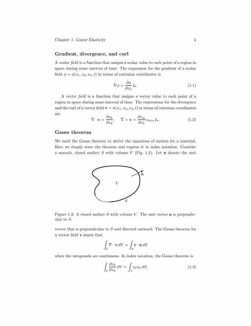
We need the Gauss theorem to derive the equations of motion for a material.Here we simply state the theorem and express it in index notation. Considera smooth, closed surface S with volume V (Fig. 1.2). Let n denote the unit
V
S
n���
Figure 1.2: A closed surface S with volume V . The unit vector n is perpendic-ular to S.
vector that is perpendicular to S and directed outward. The Gauss theorem fora vector field v states that ∫
V
∇ · v dV =∫
S
v · n dS
when the integrands are continuous. In index notation, the Gauss theorem is∫V
∂vk
∂xkdV =
∫S
vknk dS. (1.3)
Chapter 1. Linear Elasticity 5
Exercises
In the following exercises, assume that the range of the indices is 1,2,3.
Exercise 1.1 Show that δkmukvm = ukvk.Discussion—Write the equation explicitly in terms of the numerical values
of the indices and show that the right and left sides are equal. The right sideof the equation in terms of the numerical values of the indices is ukvk = u1v1 +u2v2 + u3v3.
Exercise 1.2
(a) Show that δkmekmn = 0.(b) Show that δkmδkn = δmn .
Exercise 1.3 Show that Tkmδmn = Tkn.
Exercise 1.4 If Tkmekmn = 0, show that Tkm = Tmk.
Exercise 1.5 Consider the equation
ak =∂vk
∂t+∂vk
∂xmvm.
(a) How many equations result when this equation is written explicitly in termsof the numerical values of the indices?(b) Write the equations explicitly in terms of the numerical values of the indices.
Exercise 1.6 Consider the equation
Tkm = ckmijEij.
(a) How many equations result when this equation is written explicitly in termsof the numerical values of the indices?(b) Write the equation for T11 explicitly in terms of the numerical values of theindices.
Exercise 1.7 The del operator is defined by
∇(·) =∂(·)∂x1
i1 +∂(·)∂x2
i2 +∂(·)∂x3
i3
=∂(·)∂xk
ik.(1.4)

Chapter 1. Linear Elasticity 6
The expression for the gradient of a scalar field φ in terms of cartesian coordi-nates can be obtained in a formal way by applying the del operator to the scalarfield:
∇φ =∂φ
∂xkik.
(a) By taking the dot product of the del operator with a vector field v, obtainthe expression for the divergence ∇·v in terms of cartesian coordinates. (b) Bytaking the cross product of the del operator with a vector field v, obtain theexpression for the curl ∇× v in terms of cartesian coordinates.
Exercise 1.8 By expressing the dot and cross products in terms of index no-tation, show that for any two vectors u and v,
u · (u × v) = 0.
Exercise 1.9 Show that
ukvmekmnin = det
⎡⎣ i1 i2 i3u1 u2 u3
v1 v2 v3
⎤⎦ .
Exercise 1.10 By expressing the divergence and curl in terms of index nota-tion, show that for any vector field v for which the indicated derivatives exist,
∇ · (∇× v) = 0.
Exercise 1.11 By expressing the operations on the left side of the equation interms of index notation, show that for any vector field v,
∇(∇ · v) −∇× (∇× v) =∂2vk
∂xm∂xmik.
Exercise 1.12
S
n���
Consider a smooth, closed surface S with outward-directed unit normal vector n.Show that ∫
S
n dS = 0.

Chapter 1. Linear Elasticity 7
Exercise 1.13
����dS
n
V
x1
x2
����
An object of volume V is immersed in a stationary liquid. The pressure in theliquid is po−γx2 , where po is the pressure at x2 = 0 and γ is the weight per unitvolume of the liquid. The force exerted by the pressure on an element dS of thesurface of the object is −(po − γx2)n dS, where n is an outward-directed unitvector perpendicular to the element dS. Show that the total force exerted on theobject by the pressure of the liquid is γV i2. (This result is due to Archimedes,287-212 BCE).
Chapter 1. Linear Elasticity 8
1.2 Motion
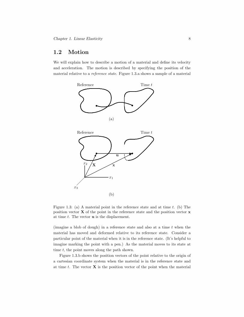
We will explain how to describe a motion of a material and define its velocityand acceleration. The motion is described by specifying the position of thematerial relative to a reference state. Figure 1.3.a shows a sample of a material
Reference Time t
Reference Time t
(a)
(b)
x1
x2
x3
xX
u
� �
��
� �
�������
�������������
Figure 1.3: (a) A material point in the reference state and at time t. (b) Theposition vector X of the point in the reference state and the position vector xat time t. The vector u is the displacement.
(imagine a blob of dough) in a reference state and also at a time t when thematerial has moved and deformed relative to its reference state. Consider aparticular point of the material when it is in the reference state. (It’s helpful toimagine marking the point with a pen.) As the material moves to its state attime t, the point moves along the path shown.
Figure 1.3.b shows the position vectors of the point relative to the origin ofa cartesian coordinate system when the material is in the reference state andat time t. The vector X is the position vector of the point when the material

Chapter 1. Linear Elasticity 9
is in the reference state and the vector x is the position vector of the point attime t. The displacement u is the position of the point at time t relative to itsposition in the reference state:
u = x− X,
or in index notation,uk = xk −Xk. (1.5)
The motion and inverse motion
To describe the motion of a material, we express the position of a point of thematerial as a function of the time and the position of that point in the referencestate:
xk = xk(Xm, t). (1.6)
The term Xm in the argument of this function means that the function candepend on the components X1, X2, and X3 of the vector X. We use a circum-flex ( ˆ ) to indicate that a function depends on the variables X and t. Thisfunction, which gives the position at time t of the point of the material thatwas at position X in the reference state, is called the motion. The position of apoint of the material in the reference state can be specified as a function of itsposition at time t and the time:
Xk = Xk(xm, t). (1.7)
This function is called the inverse motion.
Velocity and acceleration
By using Eqs. (1.5) and (1.6), we can express the displacement as a functionof X and t:
uk = xk(Xm, t) −Xk = uk(Xm, t). (1.8)
The velocity at time t of the point of the material that was at position X in thereference state is defined to be the rate of change of the position of the point:
vk =∂
∂txk(Xm, t) =
∂
∂tuk(Xm, t) = vk(Xm, t), (1.9)
The acceleration at time t of the point of the material that was at position Xin the reference state is defined to be the rate of change of its velocity:
ak =∂
∂tvk(Xm, t) = ak(Xm, t).

Chapter 1. Linear Elasticity 10
Material and spatial descriptions We have expressed the displacement,velocity, and acceleration of a point of the material in terms of the time and theposition of the point in the reference state, that is, in terms of the variables Xand t. By using the inverse motion, Eq. (1.7), we can express these quantitiesin terms of the time and the position of the point at time t, that is, in terms ofthe variables x and t. For example, we can write the displacement as
uk = uk(Xm(xn, t), t) = uk(xn, t). (1.10)
Thus the displacement u can be expressed either by the function uk(Xm, t) orby the function uk(xm, t). Expressing a quantity as a function of X and t iscalled the Lagrangian, or material description. Expressing a quantity as afunction of x and t is called the Eulerian, or spatial description. As Eq. (1.10)indicates, the value of a function does not depend on which description is used.However, when we take derivatives of a function it is essential to indicate clearlywhether it is expressed in the material or spatial description. We use a hat (ˆ)to signify that a function is expressed in the material description.
In Eq. (1.9), the velocity is expressed in terms of the time derivative of thematerial description of the displacement. Let us consider how we can expressthe velocity in terms of the spatial description of the displacement. Substitutingthe motion, Eq. (1.6), into the spatial description of the displacement, we obtainthe equation
uk = uk(xn(Xm, t), t).
To determine the velocity, we take the time derivative of this expression with Xheld fixed:
vk =∂uk
∂t+∂uk
∂xn
∂xn
∂t
=∂uk
∂t+∂uk
∂xnvn.
(1.11)
This equation contains the velocity on the right side. By replacing the index kby n, it can be written as
vn =∂un
∂t+∂un
∂xmvm.
We use this expression to replace the term vn on the right side of Eq. (1.11),obtaining the equation
vk =∂uk
∂t+∂uk
∂xn
(∂un
∂t+∂un
∂xmvm
).
Chapter 1. Linear Elasticity 11
We can now use Eq. (1.11) to replace the term vm on the right side of thisequation. Continuing in this way, we obtain the series
vk =∂uk
∂t+∂uk
∂xn
∂un
∂t+∂uk
∂xn
∂un
∂xm
∂um
∂t+ · · · (1.12)
This series gives the velocity in terms of derivatives of the spatial description ofthe displacement.
We leave it as an exercise to show that the acceleration is given in terms ofderivatives of the spatial description of the velocity by
ak =∂vk
∂t+∂vk
∂xnvn. (1.13)
The second term on the right is sometimes called the convective acceleration.
Velocity and acceleration in linear elasticity In linear elasticity, deriva-tives of the displacement are assumed to be “small,” meaning that terms con-taining products of derivatives of the displacement can be neglected. FromEqs. (1.12) and (1.13), we see that in linear elasticity, the velocity and accel-eration are related to the spatial description of the displacement by the simpleexpressions
vk =∂uk
∂t, ak =
∂2uk
∂t2. (1.14)
Exercises
Exercise 1.14
� �1 m
x1
x2
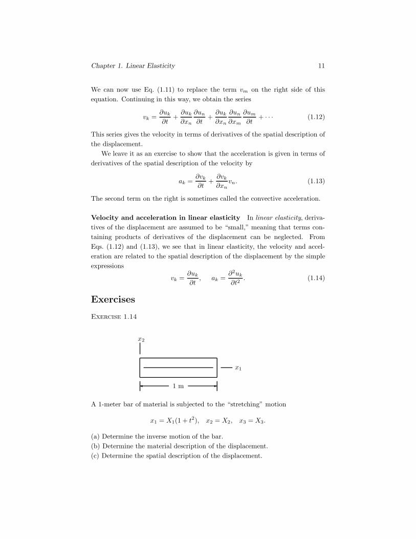
A 1-meter bar of material is subjected to the “stretching” motion
x1 = X1(1 + t2), x2 = X2, x3 = X3.
(a) Determine the inverse motion of the bar.(b) Determine the material description of the displacement.(c) Determine the spatial description of the displacement.

Chapter 1. Linear Elasticity 12
(d) What is the displacement of a point at the right end of the bar when t = 2seconds?
Answer:
(a) X1 = x1/(1 + t2), X2 = x2, X3 = x3.(b) u1 = X1t
2, u2 = 0, u3 = 0.(c) u1 = x1t
2/(1 + t2), u2 = 0, u3 = 0.(d) u1 = 4 meters, u2 = 0, u3 = 0.
Exercise 1.15 Consider the motion of the bar described in Exercise 1.14.(a) Determine the material description of the velocity.(b) Determine the spatial description of the velocity.(c) Determine the material description of the acceleration.(d) Determine the spatial description of the acceleration by substituting theinverse motion into the result of Part (c).(e) Determine the spatial description of the acceleration by using Eq. (1.13).
Answer:
(a) v1 = 2X1t, v2 = 0, v3 = 0.(b) v1 = 2x1t/(1 + t2), v2 = 0, v3 = 0.(c) a1 = 2X1, a2 = 0, a3 = 0.
(d),(e) a1 = 2x1/(1 + t2), a2 = 0, a3 = 0.
Exercise 1.16
1 m
1 mx1
x2
�
�
� �
A 1-meter cube of material is subjected to the “shearing” motion
x1 = X1 +X22 t
2, x2 = X2, x3 = X3.
(a) Determine the inverse motion of the cube.(b) Determine the material description of the displacement.(c) Determine the spatial description of the displacement.(d) What is the displacement of a point at the upper right edge of the cubewhen t = 2 seconds?

Chapter 1. Linear Elasticity 13
Answer:(a) X1 = x1 − x2
2t2, X2 = x2, X3 = x3.
(b) u1 = X22 t
2, u2 = 0, u3 = 0.(c) u1 = x2
2t2, u2 = 0, u3 = 0.
(d) u1 = 4 meters, u2 = 0, u3 = 0.
Exercise 1.17 Consider the motion of the cube described in Exercise 1.16.(a) Determine the material description of the velocity.(b) Determine the spatial description of the velocity.(c) Determine the material description of the acceleration.(d) Determine the spatial description of the acceleration by substituting theinverse motion into the result of Part (c).(e) Determine the spatial description of the acceleration by using Eq. (1.13).
Answer:(a) v1 = 2X2
2 t, v2 = 0, v3 = 0.(b) v1 = 2x2
2t, v2 = 0, v3 = 0.(c) a1 = 2X2
2 , a2 = 0, a3 = 0.(d),(e) a1 = 2x2
2, a2 = 0, a3 = 0.
Exercise 1.18 Show that the acceleration is given in terms of derivatives ofthe spatial description of the velocity by
ak =∂vk
∂t+∂vk
∂xnvn.
Discussion—Begin by substituting the motion,Eq. (1.6), into the spatialdescription of the velocity to obtain the equation
vk = vk(xn(Xm, t), t).
Then take the time derivative of this expression with X held fixed.

Chapter 1. Linear Elasticity 14
1.3 Deformation
We will discuss the deformation of a material relative to a reference state andshow that the deformation can be expressed in terms of the displacement fieldof the material. We also show how changes in the volume and density of thematerial are related to the displacement field.
Strain tensor
Suppose that a sample of material is in a reference state, and consider twoneighboring points of the material with positions X and X + dX (Fig. 1.4). At
Reference Time t
x1
x2
x3
xX
udX dx
��
� �� �
�������
������������� � ���
Figure 1.4: Two neighboring points of the material in the reference state andat time t.
time t, these two points will have some positions x and x + dx, as shown in thefigure.
In terms of the motion, Eq. (1.6), the vector dx is related to the vector dXby
dxk =∂xk
∂XmdXm. (1.15)
We denote the magnitudes of the vectors dx and dX by
|dx| = ds, |dX| = dS.
These magnitudes can be written in terms of the dot products of the vectors:
dS2 = dXkdXk,
ds2 = dxkdxk =∂xk
∂XmdXm
∂xk
∂XndXn.

Chapter 1. Linear Elasticity 15
The difference between the quantities ds2 and dS2 is
ds2 − dS2 =(∂xk
∂Xm
∂xk
∂Xn− δmn
)dXmdXn.
By using Eq. (1.5), we can write this equation in terms of the displacement u:
ds2 − dS2 =(∂um
∂Xn+
∂un
∂Xm+
∂uk
∂Xm
∂uk
∂Xn
)dXmdXn.
We can write this equation as
ds2 − dS2 = 2EmndXmdXn, (1.16)
where
Emn =12
(∂um
∂Xn+
∂un
∂Xm+
∂uk
∂Xm
∂uk
∂Xn
). (1.17)
The term Emn is called the Lagrangian strain tensor. This quantity is ameasure of the deformation of the material relative to its reference state. If itis known at a given point, we can choose any line element dX at that point inthe reference state and use Eq. (1.16) to determine its length ds at time t.
Recall that in linear elasticity it is assumed that derivatives of the displace-ment are small. We leave it as an exercise to show that in linear elasticity,
∂uk
∂Xm=∂uk
∂xm. (1.18)
Therefore in linear elasticity, the strain tensor is
Emn =12
(∂um
∂xn+∂un
∂xm
), (1.19)
which is called the linear strain tensor.
Longitudinal strain
The longitudinal strain is a measure of the change in length of a line element ina material. Here we show how the longitudinal strain in an arbitrary directioncan be expressed in terms of the strain tensor.
The longitudinal strain ε of a line element relative to a reference state isdefined to be its change in length divided by its length in the reference state.Thus the longitudinal strain of the line element dX is
ε =|dx| − |dX|
|dX| =ds− dS
dS. (1.20)

Chapter 1. Linear Elasticity 16
Reference Time t
x1
x2
x3
dX dx
n
|dX| = dS |dx| = ds
��
� �� � � �
���
Figure 1.5: The vectors dX and dx and a unit vector n in the direction of dX.
Solving this equation for ds and substituting the result into Eq. (1.16), we obtainthe relation
(2ε+ ε2)dS2 = 2EmndXmdXn. (1.21)
Let n be a unit vector in the direction of the vector dX (Fig. 1.5). We canwrite dX as
dX = dS n, or dXm = dS nm.
We substitute this relation into Eq. (1.21) and write the resulting equation inthe form
2ε+ ε2 = 2Emnnmnn. (1.22)
When the Lagrangian strain tensor Emn is known at a point in the material,we can solve this equation for the longitudinal strain ε of the line element thatis parallel to the unit vector n in the reference state.
Equation (1.22) becomes very simple in linear elasticity. If we assume that εis small, the quadratic term can be neglected and we obtain
ε = Emnnmnn. (1.23)
We can determine the longitudinal strain of the line element of the materialthat is parallel to the x1 axis in the reference state by setting n1 = 1, n2 = 0,and n3 = 0. The result is ε = E11. Thus in linear elasticity, the componentE11 of the linear strain tensor is equal to the longitudinal strain in the x1 axisdirection. Similarly, the components E22 and E33 are the longitudinal strainsin the x2 and x3 axis directions.

Chapter 1. Linear Elasticity 17
Shear strain
The shear strain is a measure of the change in the angle between two lineelements in a material relative to a reference state. Here we show how the shearstrains at a point in the material that measure the changes in angle betweenline elements that are parallel to the coordinate axes can be expressed in termsof the strain tensor at that point.
Figure 1.6 shows a point of the material at position X in the reference state
Reference Time t
x1
x2
x3
dX(1)
dX(2)π2
dx(1)
dx(2)π2− γ12
���
��� �
� ��
����
������
Figure 1.6: A point of the material and two neighboring points in the referencestate and at time t.
and two neighboring points at positions X + dX(1) and X + dX(2), where wedefine dX(1) and dX(2) by
dX(1) = dS i1, dX(2) = dS i2.
(We use parentheses around the subscripts to emphasize that they are not in-dices.) At time t, the two neighboring points will be at some positions x+dx(1)
and x + dx(2). From Eq. (1.15), we see that
dx(1) =∂xk
∂X1dS ik, dx(2) =
∂xk
∂X2dS ik. (1.24)
The angle between the vectors dX(1) and dX(2) is π/2 radians. Let us denotethe angle between the vectors dx(1) and dx(2) by π/2 − γ12. The angle γ12 isa measure of the change in the right angle between the line elements dX(1)

Chapter 1. Linear Elasticity 18
and dX(2) at time t. This angle is called the shear strain associated with theline elements dX(1) and dX(2).
We can obtain an expression relating the shear strain γ12 to the displacementby using the definition of the dot product of the vectors dx(1) and dx(2):
dx(1) · dx(2) = |dx(1)||dx(2)| cos(π/2 − γ12). (1.25)
From Eqs. (1.24), we see that the dot product of dx(1) and dx(2) is given by
dx(1) · dx(2) =∂xk
∂X1
∂xk
∂X2dS2.
By using Eq. (1.5), we can write this expression in terms of the displacement:
dx(1) · dx(2) =(∂u1
∂X2+∂u2
∂X1+∂uk
∂X1
∂uk
∂X2
)dS2
= 2E12 dS2,
(1.26)
where we have used the definition of the Lagrangian strain tensor, Eq. (1.17).Let us denote the magnitudes of the vectors dx(1) and dx(2) by |dx(1)| =
ds(1), |dx2| = ds(2). From Eq. (1.16),
ds2(1) = (1 + 2E11)dS2, ds2(2) = (1 + 2E22)dS2 .
We substitute these expressions and Eq. (1.26) into Eq. (1.25), obtaining therelation
2E12 = (1 + 2E11)1/2(1 + 2E22)1/2 cos(π/2 − γ12). (1.27)
We can use this equation to determine the shear strain γ12 when the displace-ment field is known. The term γ12 measures the shear strain between lineelements parallel to the x1 and x2 axes. The corresponding relations for theshear strain between line elements parallel to the x2 and x3 axes and for theshear strain between line elements parallel to the x1 and x3 axes are
2E23 = (1 + 2E22)1/2(1 + 2E33)1/2 cos(π/2 − γ23),
2E13 = (1 + 2E11)1/2(1 + 2E33)1/2 cos(π/2 − γ13).
In linear elasticity, the terms Emn are small. We leave it as an exercise toshow that in linear elasticity these expressions for the shear strains reduce tothe simple relations
γ12 = 2E12, γ23 = 2E23, γ13 = 2E13.
Thus in linear elasticity, the shear strains associated with line elements parallelto the coordinate axes are directly related to elements of the linear strain tensor.

Chapter 1. Linear Elasticity 19
Changes in volume and density
We will show how volume elements and the density of a material change as itdeforms. We do so by making use of a result from vector analysis. Figure 1.7shows a parallelepiped with vectors u, v, and w along its edges. The volume of
uv
w
������
���
������
���
������
���
������
����
������
�����
Figure 1.7: A parallelepiped with vectors u, v, and w along its edges.
the parallelepiped is given in terms of the three vectors by the expression
Volume = u · (v ×w) = det
⎡⎣ u1 u2 u3
v1 v2 v3w1 w2 w3
⎤⎦ . (1.28)
Now consider an element of volume dV0 of the reference state of a sample ofmaterial with the vectors
dX(1) = dS i1, dX(2) = dS i2, dX(3) = dS i3
along its edges (Fig. 1.8). At time t, the material occupying the volume dV0 inthe reference state will occupy some volume dV . From Eq. (1.15), we see thatthe vectors dx(1), dx(2), and dx(3) along the sides of the volume dV are givenin terms of the motion by
dx(1) =∂xk
∂X1dS ik, dx(2) =
∂xk
∂X2dS ik, dx(3) =
∂xk
∂X3dS ik.
From Eq. (1.28) we see that the volume dV is
dV = dx(1) · (dx(2) × dx(3)) = det
⎡⎢⎢⎢⎢⎢⎢⎢⎢⎣
∂x1
∂X1dS
∂x2
∂X1dS
∂x3
∂X1dS
∂x1
∂X2dS
∂x2
∂X2dS
∂x3
∂X2dS
∂x1
∂X3dS
∂x2
∂X3dS
∂x3
∂X3dS
⎤⎥⎥⎥⎥⎥⎥⎥⎥⎦.

Chapter 1. Linear Elasticity 20
ReferenceTime t
x1
x2
x3
dX(1)
dX(2)
dX(3)
dx(1)
dx(2)
dx(3)
dV0
dV
���
��
�� ��
���
��
����
��
����
���
������
����
����
�
�
��� ���������
���
Figure 1.8: The material occupying volume dV0 in the reference state and avolume dV at time t.
Because the volume dV0 = dS3, we can write this result as
dV = det
⎡⎢⎢⎢⎢⎢⎢⎢⎢⎣
∂x1
∂X1
∂x2
∂X1
∂x3
∂X1
∂x1
∂X2
∂x2
∂X2
∂x3
∂X2
∂x1
∂X3
∂x2
∂X3
∂x3
∂X3
⎤⎥⎥⎥⎥⎥⎥⎥⎥⎦dV0.
By using Eq. (1.5), we can write this relation in terms of the displacement field:
dV = det
⎡⎢⎢⎢⎢⎢⎢⎢⎢⎣
1 +∂u1
∂X1
∂u2
∂X1
∂u3
∂X1
∂u1
∂X21 +
∂u2
∂X2
∂u3
∂X2
∂u1
∂X3
∂u2
∂X31 +
∂u3
∂X3
⎤⎥⎥⎥⎥⎥⎥⎥⎥⎦dV0. (1.29)
When the displacement field is known, we can use this equation to determine thevolume dV at time t of an element of the material that occupied a volume dV0
in the reference state.The density ρ of a material is defined such that the mass of an element of

Chapter 1. Linear Elasticity 21
volume dV of the material at time t is
mass = ρ dV.
We denote the density of the material in the reference state by ρ0. Conservationof mass of the material requires that
ρ0 dV0 = ρ dV. (1.30)
From this relation and Eq. (1.29), we obtain an equation for the density of thematerial ρ at time t in terms of the displacement field:
ρ0
ρ= det
⎡⎢⎢⎢⎢⎢⎢⎢⎢⎣
1 +∂u1
∂X1
∂u2
∂X1
∂u3
∂X1
∂u1
∂X21 +
∂u2
∂X2
∂u3
∂X2
∂u1
∂X3
∂u2
∂X31 +
∂u3
∂X3
⎤⎥⎥⎥⎥⎥⎥⎥⎥⎦. (1.31)
In linear elasticity, products of derivatives of the displacement are neglected.Expanding the determinant in Eq. (1.29) and using Eq. (1.18), we find that inlinear elasticity the volume dV at time t is given by the simple relation
dV =(
1 +∂uk
∂xk
)dV0 = (1 + Ekk) dV0. (1.32)
From this result and Eq. (1.30), it is easy to show that in linear elasticity, thedensity of the material at time t is related to the displacement field by
ρ = (1 − Ekk) ρ0 =(
1 − ∂uk
∂xk
)ρ0. (1.33)
Exercises
Exercise 1.19
� �1 m
x1
x2

Chapter 1. Linear Elasticity 22
A 1-meter bar of material is subjected to the “stretching” motion
x1 = X1(1 + t2), x2 = X2, x3 = X3.
(a) Determine the Lagrangian strain tensor of the bar at time t.(b) Use the motion to determine the length of the bar when t = 2 seconds.(c) Use the Lagrangian strain tensor to determine the length of the bar whent = 2 seconds.
Answer: (a) The only nonzero term is E11 = t2 + 12 t
4. (b) 5 meters
Exercise 1.20
1 m
1 mx1
x2
A B
C
������
�
�
� �
An object consists of a 1-meter cube in the reference state. At time t, the valueof the linear strain tensor at each point of the object is
[Ekm] =
⎡⎣ 0.001 −0.001 0
−0.001 0.002 00 0 0
⎤⎦ .
(a) What is the length of the edge AB at time t?(b) What is the length of the diagonal AC at time t?(c) What is the angle θ at time t?
Answer: (a) 1.001 m (b) 1.0005√
2 m (c) (π/2 − 0.002) rad
Exercise 1.21 Show that in linear elasticity,
∂uk
∂Xm=∂uk
∂xm.
Discussion—Use the chain rule to write
∂uk
∂Xm=∂uk
∂xn
∂xn
∂Xm,
and use Eq. (1.5).

Chapter 1. Linear Elasticity 23
Exercise 1.22 Consider Eq. (1.27):
2E12 = (1 + 2E11)1/2(1 + 2E22)1/2 cos(π/2 − γ12).
In linear elasticity, the terms E11, E22, E12, and the shear strain γ12 are small.Show that in linear elasticity this relation reduces to
γ12 = 2E12.
Exercise 1.23 By using Eqs. (1.30) and (1.32), show that in linear elasticitythe density ρ is related to the density ρ0 in the reference state by
ρ = ρ0(1 −Ekk).
Discussion—Remember that in linear elasticity it is assumed that derivativesof the displacement are small.

Chapter 1. Linear Elasticity 24
1.4 Stress
Here we discuss the internal forces, or stresses, in materials and define the stresstensor.
Traction
Suppose that we divide a sample of material by an imaginary plane (Fig. 1.9.a)and draw the free-body diagrams of the resulting parts (Fig. 1.9.b). The material
(a)
(b)
t −t
��
����������
�����
����
���
�������
���������� ���� �� ��!"
Figure 1.9: (a) A plane passing through a sample of material. (b) The free-bodydiagrams of the parts of the material on each side of the plane.
on the right may exert forces on the material on the left at the surface definedby the plane. We can represent those forces by introducing a function t, thetraction, defined such that the force exerted on an element dS of the surface is
force = t dS.
Because an equal and opposite force is exerted on the element dS of the materialon the right by the material on the left, the traction acting on the material on

Chapter 1. Linear Elasticity 25
the right at the surface defined by the plane is −t (Fig. 1.9.b).The traction t is a vector-valued function. We can resolve it into a compo-
nent normal to the surface, the normal stress σ, and a component tangent tothe surface, the shear stress τ (Fig. 1.10). If n is a unit vector that is normal to
t
στ
��
����
����
�����
�
Figure 1.10: The traction t resolved into the normal stress σ and shear stress τ .
the surface and points outward, the normal stress σ = t ·n and the shear stressτ is the magnitude of the vector t−σn. As a simple example, if the material isa fluid at rest, the normal stress σ = −p, where p is the pressure, and the shearstress τ = 0.
Stress tensor
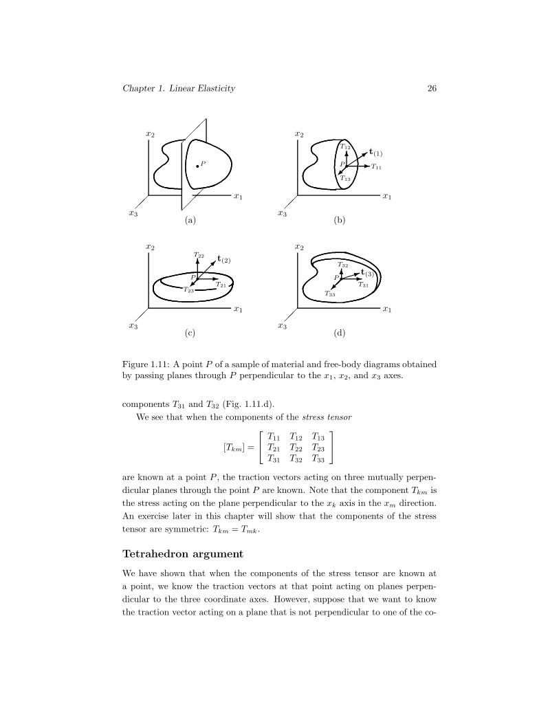
Consider a point P of a sample of material at time t. Let us introduce a cartesiancoordinate system and pass a plane through point P perpendicular to the x1 axis(Fig. 1.11.a). The free-body diagram of the material on the side of the planetoward the negative x1 direction is shown in Fig. 1.11.b. Let the traction vectoracting on the plane at point P be t(1). The component of t(1) normal to theplane—that is, the normal stress acting on the plane at point P—is called T11.The component of t(1) tangential to the plane (that is, the shear stress acting onthe plane at point P ) is decomposed into a component T12 in the x2 directionand a component T13 in the x3 direction.
Next, we pass a plane through point P perpendicular to the x2 axis. Theresulting free-body diagram is shown in Fig. 1.11.c. The traction vector t(2)
acting on the plane at point P is decomposed into the normal stress T22 andshear stress components T21 and T23. In the same way, we pass a plane throughpoint P perpendicular to the x3 axis and decompose the traction vector t(3)
acting on the plane at point P into the normal stress T33 and shear stress
Chapter 1. Linear Elasticity 26
� �
� �P P T11
T12
T13
t(1)
PT21
T22
T23
t(2)
PT31
T32
T33
t(3)
(c) (d)
(a) (b)
�� ��
�� ��
x1
x2
x3
x1
x2
x3
x1
x2
x3
x1
x2
x3
���
���
��
�����
��
���
��������
Figure 1.11: A point P of a sample of material and free-body diagrams obtainedby passing planes through P perpendicular to the x1, x2, and x3 axes.
components T31 and T32 (Fig. 1.11.d).We see that when the components of the stress tensor
[Tkm] =
⎡⎣ T11 T12 T13
T21 T22 T23
T31 T32 T33
⎤⎦
are known at a point P , the traction vectors acting on three mutually perpen-dicular planes through the point P are known. Note that the component Tkm isthe stress acting on the plane perpendicular to the xk axis in the xm direction.An exercise later in this chapter will show that the components of the stresstensor are symmetric: Tkm = Tmk.
Tetrahedron argument
We have shown that when the components of the stress tensor are known ata point, we know the traction vectors at that point acting on planes perpen-dicular to the three coordinate axes. However, suppose that we want to knowthe traction vector acting on a plane that is not perpendicular to one of the co-

Chapter 1. Linear Elasticity 27
ordinate axes. A derivation called the tetrahedron argument shows that whenthe components Tkm are known at a point P , the traction vector acting on anyplane through P can be determined.
Consider a point P of a sample of material at time t. Let us introduce atetrahedral volume with P at one vertex (Fig. 1.12.a). Three of the surfaces
(a)
x1
x2
x3
n
��P
��
���
���
����
����
��
(b)
����
ΔL
θ
n
n1
ΔS
ΔS1
���
��
������
������
��
��
��
��
��
��
�����������
�����������
��
��
���
���
��
����
�
(c)
�t
T11
T21
T31
��
��
��
��
��
��
������
����
�����������
� �
�
�������
Figure 1.12: (a) A point P of a material and a tetrahedron. (b) The tetrahedron.(c) The stresses acting on the faces.
of the tetrahedron are perpendicular to the coordinate axes, and the point Pis at the point where they intersect. The fourth surface of the tetrahedron isperpendicular to a unit vector n. Thus the unit vector n specifies the orientationof the fourth surface.
Let the area of the surface perpendicular to n be ΔS, and let the area ofthe surface perpendicular to the x1 axis be ΔS1 (Fig. 1.12.b). If we denote theangle between the unit vector n and the x1 axis by θ, the x1 component of n
Chapter 1. Linear Elasticity 28
is n1 = cos θ. Because n is perpendicular to the surface with area ΔS and thex1 axis is perpendicular to the surface with area ΔS1, the angle between thetwo surfaces is θ. Therefore
ΔS1 = ΔS cos θ
= ΔS n1.
By using the same argument for the surfaces perpendicular to the x2 and x3
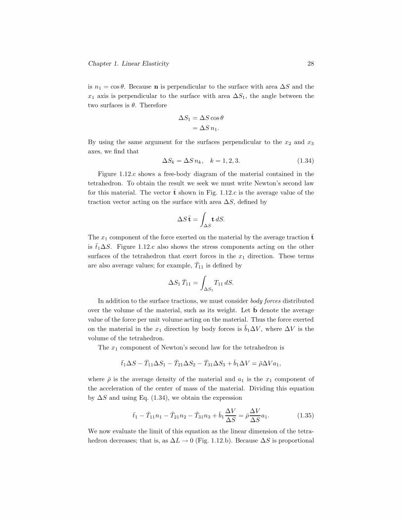
axes, we find thatΔSk = ΔS nk, k = 1, 2, 3. (1.34)
Figure 1.12.c shows a free-body diagram of the material contained in thetetrahedron. To obtain the result we seek we must write Newton’s second lawfor this material. The vector t shown in Fig. 1.12.c is the average value of thetraction vector acting on the surface with area ΔS, defined by
ΔS t =∫
ΔS
t dS.
The x1 component of the force exerted on the material by the average traction tis t1ΔS. Figure 1.12.c also shows the stress components acting on the othersurfaces of the tetrahedron that exert forces in the x1 direction. These termsare also average values; for example, T11 is defined by
ΔS1 T11 =∫
ΔS1
T11 dS.
In addition to the surface tractions, we must consider body forces distributedover the volume of the material, such as its weight. Let b denote the averagevalue of the force per unit volume acting on the material. Thus the force exertedon the material in the x1 direction by body forces is b1ΔV , where ΔV is thevolume of the tetrahedron.
The x1 component of Newton’s second law for the tetrahedron is
t1ΔS − T11ΔS1 − T21ΔS2 − T31ΔS3 + b1ΔV = ρΔV a1,
where ρ is the average density of the material and a1 is the x1 component ofthe acceleration of the center of mass of the material. Dividing this equationby ΔS and using Eq. (1.34), we obtain the expression
t1 − T11n1 − T21n2 − T31n3 + b1ΔVΔS
= ρΔVΔS
a1. (1.35)
We now evaluate the limit of this equation as the linear dimension of the tetra-hedron decreases; that is, as ΔL→ 0 (Fig. 1.12.b). Because ΔS is proportional
Chapter 1. Linear Elasticity 29
to (ΔL)2 and ΔV is proportional to (ΔL)3, the two terms in Eq. (1.35) con-taining ΔV/ΔS approach zero. The average stress components in Eq. (1.35)approach their values at point P , and the average traction vector t approachesthe value of the traction vector t at point P acting on the plane perpendicularto n. Thus we obtain the equation
t1 = T11n1 + T21n2 + T31n3.
By writing the x2 and x3 components of Newton’s second law for the materialin the same way, we find that the components of the traction vector t are
tk = Tmknm. (1.36)
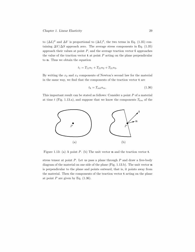
This important result can be stated as follows: Consider a point P of a materialat time t (Fig. 1.13.a), and suppose that we know the components Tkm of the
(a) (b)
P P
t
n� �
��������
Figure 1.13: (a) A point P . (b) The unit vector n and the traction vector t.
stress tensor at point P . Let us pass a plane through P and draw a free-bodydiagram of the material on one side of the plane (Fig. 1.13.b). The unit vector nis perpendicular to the plane and points outward, that is, it points away fromthe material. Then the components of the traction vector t acting on the planeat point P are given by Eq. (1.36).

Chapter 1. Linear Elasticity 30
Exercises
Exercise 1.24
x1
x2
σ0 σ0
σ0
30◦(1)
(2)
������
������
������
��
��
##
A stationary bar is subjected to uniform normal tractions σ0 at the ends (Fig. 1).As a result, the components of the stress tensor at each point of the materialare
[Tkm] =
⎡⎣ σ0 0 0
0 0 00 0 0
⎤⎦ .
(a) Determine the magnitudes of the normal and shear stresses acting on theplane shown in Fig. 2 by writing equilibrium equations for the free-body diagramshown.(b) Determine the magnitudes of the normal and shear stresses acting on theplane shown in Fig. 2 by using Eq. (1.36).
Answer: (a),(b) normal stress = σ0 cos2 30◦, shear stress = σ0 sin 30◦ cos 30◦
Exercise 1.25
x1
x2
x1
x2
θ
Plane
(1) (2)
������
The components of the stress tensor at each point of the cube of material shown

Chapter 1. Linear Elasticity 31
in Fig. 1 are
[Tkm] =
⎡⎣ T11 T12 0T12 T22 00 0 T33
⎤⎦ .
Determine the magnitudes of the normal and shear stresses acting on the planeshown in Fig. 2.
Discussion—Assume that the components of the stress tensor are symmetric:Tkm = Tmk.
Answer: normal stress = |T11 cos2 θ+T22 sin2 θ+2T12 sin θ cos θ|, shear stress= |T12(cos2 θ − sin2 θ) − (T11 − T22) sin θ cos θ|.
Exercise 1.26
(1)
��
x1
x2
x3
��
��
��
(2)
��
x1
x2
x3
��
��
$$$$
��������
����
The components of the stress tensor at each point of the cube of material shownin Fig. 1 are
[Tkm] =
⎡⎣ 100 −100 0
−100 100 00 0 300
⎤⎦ Pa.
A pascal (Pa) is 1 newton/meter2 . Determine the magnitudes of the normaland shear stresses acting on the cross-hatched plane shown in Fig. 2.
Answer: (a),(b) normal stress = 100 Pa, shear stress = 100√
2 Pa.

Chapter 1. Linear Elasticity 32
1.5 Stress-Strain Relations
We will discuss the relationship between the stresses in an elastic material andits deformation.
Linear elastic materials
An elastic material is a model for material behavior based on the assumptionthat the stress at a point in the material at a time t depends only on the strainat that point at time t. Each component of the stress tensor can be expressedas a function of the components of the strain tensor:
Tkm = Tkm(Eij).
We expand the components Tkm as power series in terms of the components ofstrain:
Tkm = bkm + ckmijEij + dkmijrsEijErs + · · · ,
where the coefficients bkm, ckmij, · · · are constants. In linear elasticity, only theterms up to the first order are retained in this expansion. In addition, we assumethat the stress in the material is zero when there is no deformation relative tothe reference state, so bkm = 0 and the relations between the stress and straincomponents for a linear elastic material reduce to
Tkm = ckmijEij. (1.37)
Isotropic linear elastic materials
If uniform normal tractions are applied to two opposite faces of a block of wood,the resulting deformation depends on the grain direction of the wood. Clearly,the deformation obtained if the grain direction is perpendicular to the two facesis different from that obtained if the grain direction is parallel to the two faces.The deformation depends on the orientation of the material. A material forwhich the relationship between stress and deformation is independent of theorientation of the material is called isotropic. Wood is an example of a materialthat is not isotropic, or anisotropic.
Equation (1.37) relating the stress and strain components in a linear elasticmaterial can be expressed in a much simpler form in the case of an isotropiclinear elastic material. A complete derivation of the relation for an isotropicmaterial is beyond the scope of this chapter, but we can demonstrate the kindsof arguments that are used.
Chapter 1. Linear Elasticity 33
If we solve Eqs. (1.37) for the strain components in terms of the stresses, wecan express the results as
Eij = hijkmTkm, (1.38)
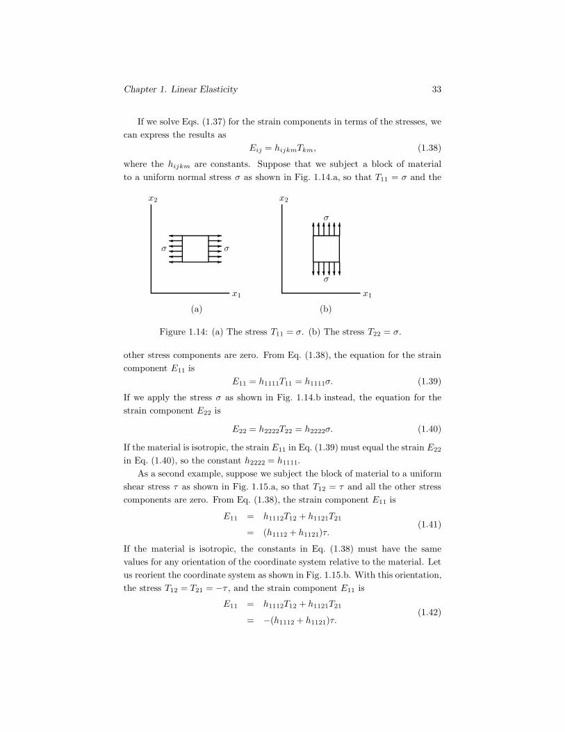
where the hijkm are constants. Suppose that we subject a block of materialto a uniform normal stress σ as shown in Fig. 1.14.a, so that T11 = σ and the
(a)
x1
x2
σ σ������
������
(b)
x1
x2
σ
σ
������
������
Figure 1.14: (a) The stress T11 = σ. (b) The stress T22 = σ.
other stress components are zero. From Eq. (1.38), the equation for the straincomponent E11 is
E11 = h1111T11 = h1111σ. (1.39)
If we apply the stress σ as shown in Fig. 1.14.b instead, the equation for thestrain component E22 is
E22 = h2222T22 = h2222σ. (1.40)
If the material is isotropic, the strain E11 in Eq. (1.39) must equal the strain E22
in Eq. (1.40), so the constant h2222 = h1111.As a second example, suppose we subject the block of material to a uniform
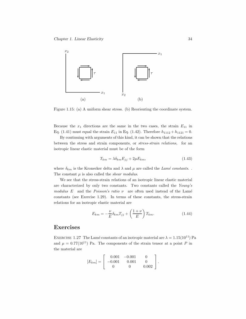
shear stress τ as shown in Fig. 1.15.a, so that T12 = τ and all the other stresscomponents are zero. From Eq. (1.38), the strain component E11 is
E11 = h1112T12 + h1121T21
= (h1112 + h1121)τ.(1.41)
If the material is isotropic, the constants in Eq. (1.38) must have the samevalues for any orientation of the coordinate system relative to the material. Letus reorient the coordinate system as shown in Fig. 1.15.b. With this orientation,the stress T12 = T21 = −τ , and the strain component E11 is
E11 = h1112T12 + h1121T21
= −(h1112 + h1121)τ.(1.42)
Chapter 1. Linear Elasticity 34
(a)
x1
x2
τ
�
�
�
�
(b)
x1
x2
τ
�
�
�
�
Figure 1.15: (a) A uniform shear stress. (b) Reorienting the coordinate system.
Because the x1 directions are the same in the two cases, the strain E11 inEq. (1.41) must equal the strain E11 in Eq. (1.42). Therefore h1112 + h1121 = 0.
By continuing with arguments of this kind, it can be shown that the relationsbetween the stress and strain components, or stress-strain relations, for anisotropic linear elastic material must be of the form
Tkm = λδkmEjj + 2μEkm, (1.43)
where δkm is the Kronecker delta and λ and μ are called the Lame constants. .The constant μ is also called the shear modulus.
We see that the stress-strain relations of an isotropic linear elastic materialare characterized by only two constants. Two constants called the Young’smodulus E and the Poisson’s ratio ν are often used instead of the Lameconstants (see Exercise 1.29). In terms of these constants, the stress-strainrelations for an isotropic elastic material are
Ekm = − ν
EδkmTjj +
(1 + ν
E
)Tkm. (1.44)
Exercises
Exercise 1.27 The Lame constants of an isotropic material are λ = 1.15(1011) Paand μ = 0.77(1011) Pa. The components of the strain tensor at a point P inthe material are
[Ekm] =
⎡⎣ 0.001 −0.001 0
−0.001 0.001 00 0 0.002
⎤⎦ .

Chapter 1. Linear Elasticity 35
Determine the components of the stress tensor Tkm at point P .Answer:
[Tkm] =
⎡⎣ 6.14(108) −1.54(108) 0
−1.54(108) 6.14(108) 00 0 7.68(108)
⎤⎦ Pa.
Exercise 1.28
x1
x2
σ0 σ0
200mm 50
mm
50 mm������
������
� � � ��
�
A bar is 200 mm in length and has a square 50 mm × 50 mm cross sectionin the unloaded state. It consists of isotropic material with Lame constantsλ = 4.5(1010) Pa and μ = 3.0(1010) Pa. The ends of the bar are subjected to auniform normal traction σ0 = 2.0(108) Pa. As a result, the components of thestress tensor at each point of the material are
[Tkm] =
⎡⎣ 2.0(108) 0 0
0 0 00 0 0
⎤⎦ Pa.
(a) Determine the length of the bar in the loaded state.(b) Determine the dimensions of the square cross section of the bar in the loadedstate.
Answer: (a) 200.513 mm. (b) 49.962 mm×49.962 mm.
Exercise 1.29
x1
x2
T11 T11������
������
The ends of a bar of isotropic material are subjected to a uniform normal tractionT11. As a result, the components of the stress tensor at each point of the materialare
[Tkm] =
⎡⎣ T11 0 0
0 0 00 0 0
⎤⎦ .
Chapter 1. Linear Elasticity 36
(a) The ratio E of the stress T11 to the longitudinal strainE11 in the x1 direction,
E =T11
E11,
is called the Young’s modulus, or modulus of elasticity of the material. Showthat the Young’s modulus is related to the Lame constants by
E =μ(3λ + 2μ)λ+ μ
(b) The ratio
ν = −E22
E11
is called the Poisson’s ratio of the material. Show that the Poisson’s ratio isrelated to the Lame constants by
ν =λ
2(λ + μ)
Exercise 1.30 The Young’s modulus and Poisson’s ratio of an elastic materialare defined in Exercise 1.29. Show that the Lame constants of an isotropicmaterial are given in terms of the Young’s modulus and Poisson’s ratio of thematerial by
λ =νE
(1 + ν)(1 − 2ν), μ =
E
2(1 + ν).
Discussion—See Exercise 1.29.
Exercise 1.31 Show that the strain components of an isotropic linear elasticmaterial are given in terms of the stress components by
Ekm =12μTkm − λ
2μ(3λ + 2μ)δkmTjj.
Chapter 1. Linear Elasticity 37
1.6 Balance and Conservation Equations
We now derive the equations of conservation of mass, balance of linear mo-mentum, and balance of angular momentum for a material. Substituting thestress-strain relation for an isotropic linear elastic material into the equation ofbalance of linear momentum, we obtain the equations that govern the motionof such materials.
Transport theorem
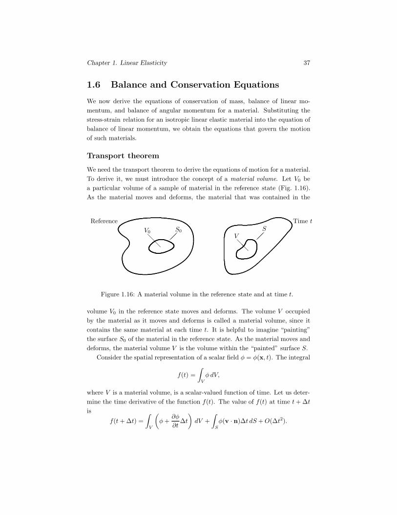
We need the transport theorem to derive the equations of motion for a material.To derive it, we must introduce the concept of a material volume. Let V0 bea particular volume of a sample of material in the reference state (Fig. 1.16).As the material moves and deforms, the material that was contained in the
Reference Time tV0 S0
VS
�� ��
��
��
Figure 1.16: A material volume in the reference state and at time t.
volume V0 in the reference state moves and deforms. The volume V occupiedby the material as it moves and deforms is called a material volume, since itcontains the same material at each time t. It is helpful to imagine “painting”the surface S0 of the material in the reference state. As the material moves anddeforms, the material volume V is the volume within the “painted” surface S.
Consider the spatial representation of a scalar field φ = φ(x, t). The integral
f(t) =∫
V
φ dV,
where V is a material volume, is a scalar-valued function of time. Let us deter-mine the time derivative of the function f(t). The value of f(t) at time t+ Δtis
f(t + Δt) =∫
V
(φ+
∂φ
∂tΔt
)dV +
∫S
φ(v · n)Δt dS +O(Δt2).

Chapter 1. Linear Elasticity 38
n
v S at time tS at time t+ Δt
��� ��
$$% �
Figure 1.17: The motion of the surface S from t to t+ Δt.
The second term on the right accounts for the motion of the surface S duringthe interval of time from t to t + Δt (Fig. 1.17). The symbol O(Δt2) means“terms of order two or higher in Δt”. The time derivative of f(t) is
df(t)dt
= limΔt→0
f(t + Δt) − f(t)Δt
=∫
V
∂φ
∂tdV +
∫S
φvknk dS.
By applying the Gauss theorem to the surface integral in this expression, weobtain
df(t)dt
=d
dt
∫V
φ dV =∫
V
[∂φ
∂t+∂(φvk)∂xk
]dV. (1.45)
This result is the transport theorem. We use it in the following sections toderive the equations describing the motion of a material.
Conservation of mass
Because a material volume contains the same material at each time t, the totalmass of the material in a material volume is constant:
d
dt
∫V
ρ dV = 0.
By using the transport theorem, we obtain the result∫V
[∂ρ
∂t+∂(ρvk)∂xk
]dV = 0.
This equation must hold for every material volume of the material. If we as-sume that the integrand is continuous, the equation can be satisfied only if the
Chapter 1. Linear Elasticity 39
integrand vanishes at each point:
∂ρ
∂t+∂(ρvk)∂xk
= 0. (1.46)
This is one form of the equation of conservation of mass for a material.
Balance of linear momentum
Newton’s second law states that the force acting on a particle is equal to therate of change of its linear momentum:
F =d
dt(mv). (1.47)
The equation of balance of linear momentum for a material is obtained bypostulating that the rate of change of the total linear momentum of the materialcontained in a material volume is equal to the total force acting on the materialvolume:
d
dt
∫V
ρv dV =∫
S
t dS +∫
V
b dV.
The first term on the right is the force exerted on the surface S by the tractionvector t. The second term on the right is the force exerted on the material bythe body force per unit volume b. Writing this equation in index notation andusing Eq. (1.36) to express the traction vector in terms of the components ofthe stress tensor, we obtain
d
dt
∫V
ρvm dV =∫
S
Tmknk dS +∫
V
bm dV. (1.48)
We leave it as an exercise to show that by using the Gauss theorem, the trans-port theorem, and the equation of conservation of mass, this equation can beexpressed in the form ∫
V
(ρam − ∂Tmk
∂xk− bm
)dV = 0, (1.49)
wheream =
∂vm
∂t+∂vm
∂xkvk
is the acceleration. Equation (1.49) must hold for every material volume of thematerial. If we assume that the integrand is continuous, we obtain the equation
ρam =∂Tmk
∂xk+ bm. (1.50)
This is the equation of balance of linear momentum for a material.

Chapter 1. Linear Elasticity 40
Balance of angular momentum
Taking the cross product of Newton’s second law for a particle with the positionvector x of the particle, we can write the result as
x ×F = x× d
dt(mv)
=d
dt(x ×mv).
The term on the left is the moment exerted by the force F about the origin.The term x ×mv is called the angular momentum of the particle. Thus thisequation states that the moment is equal to the rate of change of the angularmomentum.
The equation of balance of angular momentum for a material is obtainedby postulating that the rate of change of the total angular momentum of thematerial contained in a material volume is equal to the total moment exertedon the material volume:
d
dt
∫V
x× ρv dV =∫
S
x × t dS +∫
V
x× b dV.
We leave it as an exercise to show that this postulate implies that the stresstensor is symmetric:
Tkm = Tmk.
Exercises
Exercise 1.32 By using the Gauss theorem, the transport theorem, and theequation of conservation of mass, show that Eq. (1.48),
d
dt
∫V
ρvm dV =∫
S
Tmknk dS +∫
V
bm dV,
can be expressed in the form∫V
(ρam − ∂Tmk
∂xk− bm
)dV = 0,
where am is the acceleration of the material.
Exercise 1.33 Show that the postulate of balance of angular momentum fora material
d
dt
∫V
x× ρv dV =∫
S
x× t dS +∫
V
x× b dV
implies that the stress tensor is symmetric:
Tkm = Tmk.

Chapter 1. Linear Elasticity 41
Exercise 1.34 For a stationary material, the postulate of balance of energy is
d
dt
∫V
ρe dV = −∫
S
qjnj dS,
where V is a material volume with surface S. The term e is the internal energyand qj is the heat flux vector. Suppose that the internal energy and the heatflux vector are related to the absolute temperature T of the material by theequations
e = cT, qj = −k ∂T∂xj
,
where the specific heat c and the thermal conductivity k are constants. Showthat the absolute temperature is governed by the heat transfer equation
∂T
∂t=
k
ρc
∂2T
∂xj∂xj.

Chapter 1. Linear Elasticity 42
1.7 Equations of Motion
The balance and conservation equations and the stress-strain relation can beused to derive the equations of motion for a linear elastic material. We begin byobtaining equations of motion that are expressed in terms of the displacementof the material.
Displacement equations of motion
The equation of balance of linear momentum for a material is
ρam =∂Tmk
∂xk. (1.51)
Notice that we do not include the body force term. In many elastic wave propa-gation problems the body force does not have a significant effect, and we neglectit in the following development.
Recall that in linear elasticity it is assumed that derivatives of the displace-ment are small. In this case we can express the acceleration in terms of thedisplacement using Eq. (1.14),
am =∂2um
∂t2,
and express the density in terms of the density in the reference state and thedivergence of the displacement using Eq. (1.33):
ρ = ρ0
(1 − ∂uk
∂xk
).
From these two equations, we see that in linear elasticity, the product of thedensity and the acceleration can be expressed as
ρam = ρ0∂2um
∂t2. (1.52)
The stress-strain relation for an isotropic linear elastic material is given byEq. (1.43),
Tmk = λδmkEjj + 2μEmk,
and the components of the linear strain tensor are related to the components ofthe displacement by Eq. (1.19):
Emk =12
(∂um
∂xk+∂uk
∂xm
).

Chapter 1. Linear Elasticity 43
Substituting this expression into the stress-strain relation, we obtain the stresscomponents in terms of the components of the displacement:
Tmk = λδmk∂uj
∂xj+ μ
(∂um
∂xk+∂uk
∂xm
).
Then by substituting this expression and Eq. (1.52) into the equation of balanceof linear momentum, Eq. (1.51), we obtain the equation of balance of linearmomentum for an isotropic linear elastic material:
ρ0∂2um
∂t2= (λ + μ)
∂2uk
∂xk∂xm+ μ
∂2um
∂xk∂xk. (1.53)
By introducing the cartesian unit vectors, we can write this equation as thevector equation
ρ0∂2um
∂t2im = (λ + μ)
∂
∂xm
(∂uk
∂xk
)im + μ
∂2um
∂xk∂xkim.
We can express this equation in vector notation as
ρ0∂2u∂t2
= (λ + μ)∇(∇ · u) + μ∇2u. (1.54)
The second term on the right side is called the vector Laplacian of u. It can bewritten in the form (see Exercise 1.11)
∇2u = ∇(∇ · u) −∇× (∇× u). (1.55)
Substituting this expression into Eq. (1.54), we obtain
ρ0∂2u∂t2
= (λ + 2μ)∇(∇ · u) − μ∇× (∇× u). (1.56)
Equations (1.53) and (1.56) express the equation of balance of linear momen-tum for isotropic linear elasticity in index notation and in vector notation. Bothforms are useful. One advantage of the vector form is that it is convenient forexpressing the equation in terms of various coordinate systems. These equationsare called the displacement equations of motion because they are expressed interms of the displacement of the material.
Helmholtz decomposition
In the Helmholtz decomposition, the displacement field of a material is ex-pressed as the sum of the gradient of a scalar potential φ and the curl of avector potential ψ:
u = ∇φ+ ∇× ψ. (1.57)

Chapter 1. Linear Elasticity 44
Substituting this expression into the equation of balance of linear momentum,Eq. (1.56), and using Eq. (1.55), we can write the equation of balance of linearmomentum in the form
∇[ρ0∂2φ
∂t2− (λ + 2μ)∇2φ
]
+∇×[ρ0∂2ψ
∂t2− μ∇2ψ
]= 0.
We see that the equation of balance of linear momentum is satisfied if thepotentials φ and ψ satisfy the equations
∂2φ
∂t2= α2∇2φ (1.58)
and∂2ψ
∂t2= β2∇2ψ, (1.59)
where the constants α and β are defined by
α =(λ+ 2μρ0
)1/2
, β =(μ
ρ0
)1/2
.
Equation (1.58) is called the wave equation. When it is expressed in termsof cartesian coordinates, Eq. (1.59) becomes three wave equations, one for eachcomponent of the vector potential ψ. Because these equations are simpler inform than the displacement equations of motion, many problems in elastic wavepropagation are approached by first expressing the displacement field in termsof the Helmholtz decomposition.
Acoustic medium
Setting the shear modulus μ = 0 in the equations of linear elasticity yields theequations for an elastic medium that does not support shear stresses, or anelastic inviscid fluid. These equations are used to analyze sound propagationor acoustic problems, and we therefore refer to an elastic inviscid fluid as anacoustic medium. In this case, the equation of balance of linear momentum,Eq. (1.56), reduces to
ρ0∂2u∂t2
= λ∇(∇ · u).
The displacement vector can be expressed in terms of the scalar potential φ,
u = ∇φ,

Chapter 1. Linear Elasticity 45
and it is easy to show that the equation of balance of linear momentum issatisfied if φ satisfies the wave equation
∂2φ
∂t2= α2∇2φ,
where the constant α is defined by
α =(λ
ρ0
)1/2
.
The constant λ is called the bulk modulus of the fluid. Thus acoustic problemsare governed by a wave equation expressed in terms of one scalar variable.
Exercises
Exercise 1.35 By substituting the Helmholtz decomposition u = ∇φ+∇×ψinto the equation of balance of linear momentum, Eq. (1.56), show that thelatter equation can be written in the form
∇[ρ0∂2φ
∂t2− (λ + 2μ)∇2φ
]+ ∇×
[ρ0∂2ψ
∂t2− μ∇2ψ
]= 0.
Exercise 1.36 We define an acoustic medium on page 44. Show that thedensity ρ of an acoustic medium is governed by the wave equation
∂2ρ
∂t2= α2∇2ρ.
Discussion—See Exercise 1.33.

Chapter 1. Linear Elasticity 46
1.8 Summary
We will briefly summarize the equations that govern the motion of an isotropiclinear elastic material.
Displacement equations of motion
The displacement equations of motion for an isotropic linear elastic material inindex notation are (Eq. (1.53))
ρ0∂2um
∂t2= (λ + μ)
∂2uk
∂xk∂xm+ μ
∂2um
∂xk∂xk. (1.60)
They can be expressed in vector notation as (Eq. (1.53))
ρ0∂2u∂t2
= (λ + 2μ)∇(∇ · u) − μ∇× (∇× u). (1.61)
The vector u is the displacement of the material relative to the reference state.The scalar ρ0 is the density of the material in the reference state. The con-stants λ and μ are the Lame constants of the material. The Lame constants arerelated to the Young’s modulus E and Poisson’s ratio ν of the material by (seeExercise 1.30)
λ =νE
(1 + ν)(1 − 2ν), μ =
E
2(1 + ν).
Helmholtz decomposition
The Helmholtz decomposition of the displacement vector u is [Eq. (1.57)]
u = ∇φ+ ∇× ψ, (1.62)
where φ is a scalar potential and ψ is a vector potential. The displacementequations of motion are satisfied if the potentials φ and ψ satisfy the equations(Eqs. (1.58) and (1.59))
∂2φ
∂t2= α2∇2φ (1.63)
and∂2ψ
∂t2= β2∇2ψ, (1.64)
where the constants α and β are defined by
α =(λ+ 2μρ0
)1/2
, β =(μ
ρ0
)1/2
. (1.65)

Chapter 1. Linear Elasticity 47
Strain tensor and density
The components of the linear strain tensor Ekm are related to the componentsof the displacement vector by (Eq. (1.19))
Ekm =12
(∂uk
∂xm+∂um
∂xk
). (1.66)
The density ρ of the material is related to its density ρ0 in the referencestate by (Eq. (1.33))
ρ = ρ0(1 −Ejj) = ρ0
(1 − ∂uj
∂xj
). (1.67)
Stress-strain relation
In isotropic linear elasticity, the components of the stress tensor Tkm are relatedto the components of the strain tensor by (Eq. (1.43))
Tkm = λδkmEjj + 2μEkm, (1.68)
where λ and μ are the Lame constants of the material.
Traction
If a plane is passed through a point p of a sample of material and a free-bodydiagram is drawn of the material on one side of the plane, the traction t exertedon the plane at point p (Fig. 1.13) is given in terms of the components of thestress tensor at p by (Eq. (1.36))
tk = Tkmnm. (1.69)
Chapter 2
One-Dimensional Waves
When you see straight, parallel waves approach a beach, you areobserving one-dimensional waves. The heights of the waves dependon time and a single spatial variable, the distance perpendicular tothe beach. We begin our discussion of waves in elastic materialswith one-dimensional waves because they are simple both from theintuitive and theoretical points of view. After introducing the one-dimensional wave equation and deriving its general solution, we showthat this equation governs one-dimensional motions of an elasticmaterial. To aid in visualizing solutions, we demonstrate that thesame equation also governs lateral disturbances in a stretched string.We obtain solutions to several important problems, including thereflection of a wave at the interface between two elastic materials.We present examples of the use of characteristics to solve simpleone-dimensional problems, then apply them to materials consistingof multiple layers.
2.1 One-Dimensional Wave Equation
The one-dimensional wave equation,
∂2u
∂t2= α2∂
2u
∂x2, (2.1)
is a second-order partial differential equation in one dependent variable u andtwo independent variables t and x. The term α is a constant. We will showthat this equation has the remarkable property that its general solution canbe obtained by expressing the equation in terms of the independent variables
48

Chapter 2. One-Dimensional Waves 49
ξ = x − αt and η = x + αt. The dependent variable u can be expressed eitheras a function of the variables x, t or of the variables ξ, η:
u = u(x, t) = u(ξ, η).
By using the chain rule, we can write the partial derivative of u with respectto t as
∂u
∂t=
∂ξ
∂t
∂u
∂ξ+∂η
∂t
∂u
∂η
= −α∂u∂ξ
+ α∂u
∂η.
Then we apply the chain rule again to determine the second partial derivativeof u with respect to t in terms of derivatives with respect to ξ and η:
∂2u
∂t2=
∂
∂t
(−α∂u
∂ξ+ α
∂u
∂η
)
=∂ξ
∂t
∂
∂ξ
(−α∂u
∂ξ+ α
∂u
∂η
)
+∂η
∂t
∂
∂η
(−α∂u
∂ξ+ α
∂u
∂η
)
= α2
(∂2u
∂ξ2− 2
∂2u
∂ξ∂η+∂2u
∂η2
).
The second partial derivative of u with respect to x in terms of derivatives withrespect to ξ and η can be obtained in the same way. The result is
∂2u
∂x2=∂2u
∂ξ2+ 2
∂2u
∂ξ∂η+∂2u
∂η2.
Substituting these expressions for the second partial derivatives of u into Eq. (2.1),we obtain the one-dimensional wave equation in the form
∂2u
∂ξ∂η= 0.
We can integrate this equation twice to obtain its general solution. Integratingwith respect to η yields
∂u
∂ξ= h(ξ),
where h(ξ) is an arbitrary function of ξ. Then integrating with respect to ξ
gives the solution
u =∫h(ξ) dξ + g(η),
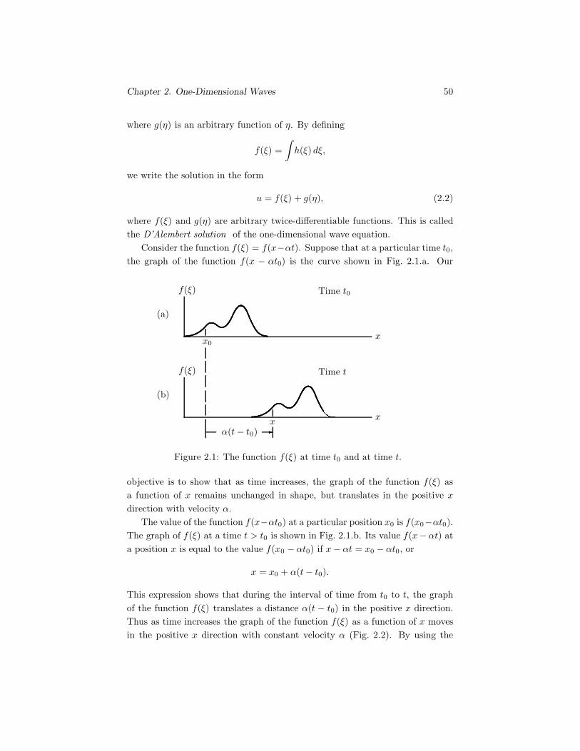
Chapter 2. One-Dimensional Waves 50
where g(η) is an arbitrary function of η. By defining
f(ξ) =∫h(ξ) dξ,
we write the solution in the form
u = f(ξ) + g(η), (2.2)
where f(ξ) and g(η) are arbitrary twice-differentiable functions. This is calledthe D’Alembert solution of the one-dimensional wave equation.
Consider the function f(ξ) = f(x−αt). Suppose that at a particular time t0,the graph of the function f(x − αt0) is the curve shown in Fig. 2.1.a. Our
(a)
x
f(ξ) Time t0
x0
(b)
x
f(ξ) Time t
xα(t− t0) �
Figure 2.1: The function f(ξ) at time t0 and at time t.
objective is to show that as time increases, the graph of the function f(ξ) asa function of x remains unchanged in shape, but translates in the positive xdirection with velocity α.
The value of the function f(x−αt0) at a particular position x0 is f(x0−αt0).The graph of f(ξ) at a time t > t0 is shown in Fig. 2.1.b. Its value f(x−αt) ata position x is equal to the value f(x0 − αt0) if x− αt = x0 − αt0, or
x = x0 + α(t− t0).
This expression shows that during the interval of time from t0 to t, the graphof the function f(ξ) translates a distance α(t − t0) in the positive x direction.Thus as time increases the graph of the function f(ξ) as a function of x movesin the positive x direction with constant velocity α (Fig. 2.2). By using the
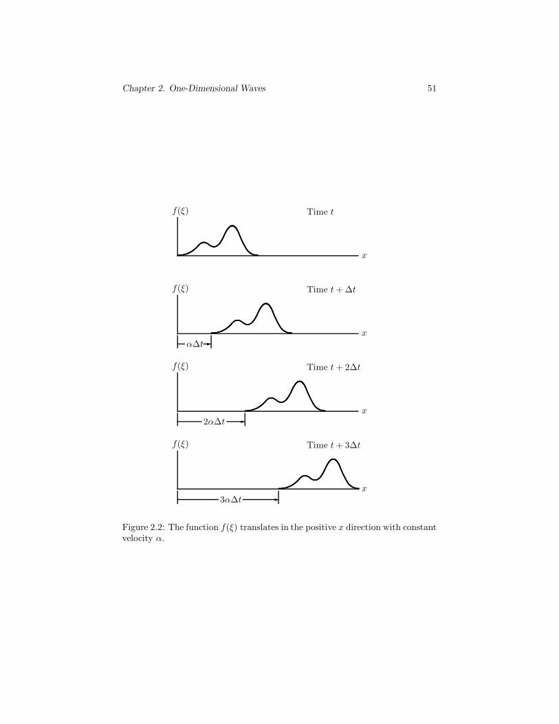
Chapter 2. One-Dimensional Waves 51
x
f(ξ) Time t
x
f(ξ) Time t + Δt
αΔt�
x
f(ξ) Time t + 2Δt
2αΔt �
x
f(ξ) Time t + 3Δt
3αΔt �
Figure 2.2: The function f(ξ) translates in the positive x direction with constantvelocity α.

Chapter 2. One-Dimensional Waves 52
same argument, we can show that the graph of the function g(η) as a functionof x translates in the negative x direction with constant velocity α.
The behavior of the functions f(ξ) and g(η) agrees with our intuitive notionof a wave. Roughly speaking, a wave is a disturbance in a medium that movesor propagates through the medium. The functions f(ξ) and g(η) describe wavesthat propagate in the positive and negative x directions with constant velocityor wave speed α. This explains why Eq. (2.1) is called the one-dimensional waveequation. In the next section, we show that one-dimensional disturbances in alinear elastic material are governed by this equation.
Exercises
Exercise 2.1 A function f(x) is defined by
x < 0 f(x) = 0,
0 ≤ x ≤ 1 f(x) = sin(πx),
x > 1 f(x) = 0.
Plot the function f(ξ) = f(x − αt) as a function of x for t = 0, t = 1 s, andt = 2 s if α = 1.
Exercise 2.2 Show that as time increases, the graph of the function g(η) =g(x+αt) as a function of x translates in the negative x direction with constantvelocity α.
Exercise 2.3 By using the chain rule, show that the second partial derivativeof u = u(x, t) with respect to x can be expressed in terms of partial derivativesof u = u(ξ, η) by
∂2u
∂x2=∂2u
∂ξ2+ 2
∂2u
∂ξ∂η+∂2u
∂η2.
Exercise 2.4 Show that the D’Alembert solution u = f(ξ) + g(η), where ξ =x− αt and η = x+ αt, is a solution of the one-dimensional wave equation
∂2u
∂t2= α2∂
2u
∂x2.
Discussion—Substitute the solution into the equation and show that theequation is satisfied. Use the chain rule to evaluate the derivatives.
Exercise 2.5 Consider the expression
u = Aei(kx − ωt).

Chapter 2. One-Dimensional Waves 53
What conditions must the constants A, k, and ω satisfy in order for this expres-sion to be a solution of the one-dimensional wave equation?
Exercise 2.6 Consider the first-order partial differential equation
∂u
∂t+ α
∂u
∂x= 0,
where α is a constant. By expressing it in terms of the independent variablesξ = x− αt and η = x+ αt, show that its general solution is
u = f(ξ),
where f is an arbitrary twice-differentiable function.

Chapter 2. One-Dimensional Waves 54
2.2 One-Dimensional Motions of an Elastic Ma-terial
We will describe two kinds of one-dimensional motion that can occur in anelastic material and show that they are governed by the one-dimensional waveequation.
Compressional waves
Figure 2.3.a shows a half space of material. The material is assumed to beunbounded to the right of the infinite plane boundary. A cartesian coordinatesystem is oriented with the positive x1 direction pointing into the material andthe x2-x3 plane coincident with the boundary of the half space.
x1
x2
(a)
x1
x2
(b)
u1(0, t) = p(t)
�������
x1
x2
(c)
T11(0, t) = p(t)
�������
Figure 2.3: (a) A half space of material. (b) Displacement boundary condition.(c) Normal stress boundary condition.
The motion of the material is specified by its displacement field u = u(x, t).Suppose that the half space of material is initially undisturbed, that is, u(x, t) =0 for t ≤ 0, and we give the boundary a uniform motion in the x1 directiondescribed by the equation
u1(0, t) = p(t), (2.3)
where p(t) is a prescribed function of time that vanishes for t ≤ 0 (Fig. 2.3.b).This is called a displacement boundary condition. The displacement of theboundary is specified as a function of time. The resulting motion of the material

Chapter 2. One-Dimensional Waves 55
is described by the displacement field
u1 = u1(x1, t),u2 = 0,u3 = 0.
(2.4)
Because the motion of the boundary in the x1 direction is uniform—that is, itis the same at each point of the boundary—the resulting motion of the materialcannot depend on x2 or x3, and the material has no motion in the x2 or x3
directions. Each point of the material moves only in the x1 direction. This isa one-dimensional motion: it depends on only one spatial dimension and thetime.
For the one-dimensional motion described by Eq. (2.4), the displacementequation of motion, Eq. (1.60), reduces to
∂2u1
∂t2= α2∂
2u1
∂x21
,
where the constant α is defined by Eq. (1.65). We see that one-dimensionalmotions of a linear elastic material described by Eq. (2.4) are governed by theone-dimensional wave equation with wave speed
α =(λ+ 2μρ0
)1/2
.
Waves of this type are called compressional, or P waves, and α is called thecompressional, or P wave speed. Figure 2.4.a shows an array of materialpoints in the undisturbed half space. Figure 2.4.b shows the displacements ofthe material points at a time t resulting from a compressional wave. The pointsmove only in the x1 direction, and their motions depend only on x1 and t.From Eq. (1.67), we see that in a compressional wave described by Eq. (2.4),the density of the material is given by
ρ = ρ0
(1 − ∂u1
∂x1
).
Compressional waves described by Eq. (2.4) are also obtained if the boundaryof the undisturbed half space is subjected to a uniform normal stress describedby the equation
T11(0, t) = p(t),
where p(t) is a prescribed function of time that vanishes for t ≤ 0 (Fig. 2.3.c).This is called a stress boundary condition. The stress on the boundary is

Chapter 2. One-Dimensional Waves 56
x1
x2
(a)
� � � � � � � �� � � � � � � �
� � � � � � � �
x1
x2
(b)���������
���
���
���
���
���
���
���
���
�
�
�
�
�
�
�
�
�
"
"
"
"
"
"
"
"
"
"
"
"
Figure 2.4: (a) An array of points in the undisturbed half space. (b) Displace-ments of the points due to a compressional wave.

Chapter 2. One-Dimensional Waves 57
specified as a function of time. By using the stress-strain relation, Eq. (1.68),this boundary condition can be expressed in terms of the displacement:
∂u1
∂x1(0, t) = p(t),
wherep(t) =
1λ+ 2μ
p(t). (2.5)
If the boundary is free, meaning that the applied stress is zero, the boundarycondition is
∂u1
∂x1(0, t) = 0.
Shear waves
Suppose that the half space of material shown in Fig. 2.5.a is initially undis-turbed and we give the boundary a uniform motion in the x2 direction describedby the equation
u2(0, t) = p(t), (2.6)
where p(t) is a prescribed function of time that vanishes for t ≤ 0 (Fig. 2.5.b).The resulting motion of the material is described by the displacement field
x1
x2
(a)
x1
x2
(b)
u2(0, t) = p(t)
�
�
�
x1
x2
(c)
T12(0, t) = p(t)
�
�
�
Figure 2.5: (a) A half space of material. (b) Displacement boundary condition.(c) Shear stress boundary condition.
u1 = 0,u2 = u2(x1, t),u3 = 0.
(2.7)

Chapter 2. One-Dimensional Waves 58
Because the motion of the boundary in the x2 direction is uniform, the resultingmotion of the material does not depend on x2 or x3, and each point of thematerial moves only in the x2 direction.
For one-dimensional motions described by Eq. (2.7), the displacement equa-tion of motion, Eq. (1.60), reduces to
∂2u2
∂t2= β2 ∂
2u2
∂x21
,
where the constant β is defined by Eq. (1.65). We see that one-dimensionalmotions of a linear elastic material described by Eq. (2.7) are governed by theone-dimensional wave equation with wave velocity
β =(μ
ρ0
)1/2
. (2.8)
Waves of this type are called shear waves, or S waves, and β is called the shearwave or S wave speed. Figure 2.6.a shows an array of material points in theundisturbed half space. Figure 2.6.b shows the displacements of the materialpoints at a time t resulting from a shear wave. The points move only in thex2 direction, and their motions depend only on x1 and t. From Eq. (1.67), thedensity of the material in a shear wave described by Eq. (2.7) is given by
ρ = ρ0.
Thus the density of the material is unchanged by a one-dimensional shear wave.Shear waves described by Eq. (2.7) are also obtained if we subject the bound-
ary of the undisturbed half space to a uniform shear stress described by theequation
T12(0, t) = p(t),
where p(t) is a prescribed function of time that vanishes for t ≤ 0 (Fig. 2.5.c).By using the stress-strain relation, this boundary condition can be expressed interms of the displacement:
∂u2
∂x1(0, t) = p(t), (2.9)
wherep(t) =
1μp(t).
If the boundary is free, the boundary condition is
∂u2
∂x1(0, t) = 0.

Chapter 2. One-Dimensional Waves 59
x1
x2
(a)
� � � � � � � �� � � � � � � �
� � � � � � � �
x1
x2
(b)
�
�
�
���
���
���
���
���
���
���
���
�
�
�
�
�
�
�
�
�
&
&
&
&
&
&
&
&
&
&
&
&
Figure 2.6: (a) An array of points in the undisturbed half space. (b) Displace-ments of the points due to a shear wave.

Chapter 2. One-Dimensional Waves 60
2.3 Motion of a String
We will show that small lateral motions of a stretched string are governed by theone-dimensional wave equation. This problem has important practical applica-tions, for example in explaining the behaviors of stringed musical instruments.However, the reason we discuss it here is that waves in a string are easier tovisualize than one-dimensional compressional and shear waves in an elastic ma-terial. In addition to the governing equation being identical, we will show thatthe boundary conditions discussed in the previous section for one-dimensionalwaves in an elastic half space have equivalents in the lateral motion of a string.As a result, the motion of a string makes an excellent analog for visualizingone-dimensional waves in elastic materials.
Equation of motion
Consider a string that is stretched between two points (Fig. 2.7.a). We candescribe the lateral motion of the string in terms of its lateral displacement u =u(x, t) relative to the equilibrium position, where x is the position (Fig. 2.7.b).
Figure 2.7.c shows a free-body diagram of an element of the string of length ds.We assume the tension T of the string to be uniform. The angle θ is the anglebetween the centerline of the string and the x axis. Newton’s second law for thelateral motion of the string is
sin(θ +
∂θ
∂xdx
)− T sin θ = (ρL ds)
∂2u
∂t2,
where ρL is the mass per unit length of the string. Expanding the first term onthe left side in a Taylor series, we obtain the equation
T∂θ
∂xdx = ρL
∂2u
∂t2ds. (2.10)
We can write the length of the element ds in terms of dx:
ds = (dx2 + du2)1/2 =
[1 +
(∂u
∂x
)2]1/2
dx.
If we assume that the term ∂u/∂x (the slope of the string relative to the x axis)is small, then ds = dx and θ = ∂u/∂x. Therefore we can write Eq. (2.10) in theform
∂2u
∂t2= α2∂
2u
∂x2, (2.11)
where
α =(T
ρL
)1/2
.
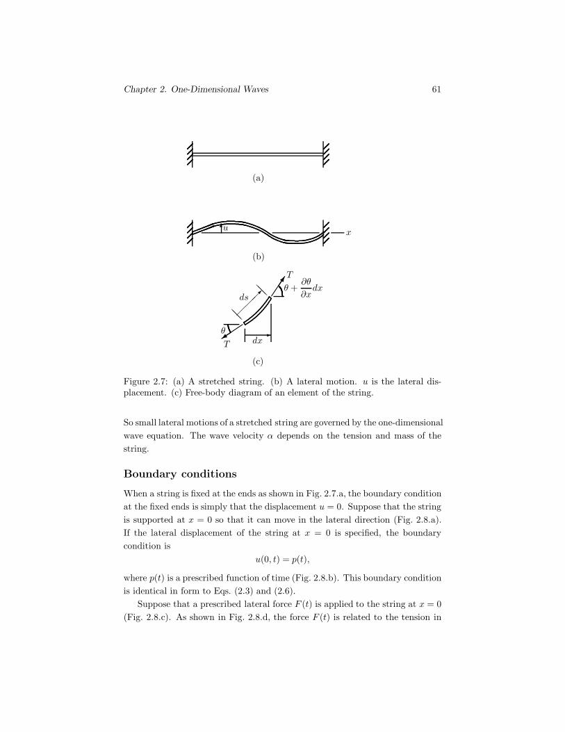
Chapter 2. One-Dimensional Waves 61
(a)
(b)
ux�
(c)
dx
ds
T
T
θ
θ +∂θ
∂xdx
�
��
��
���� �
���
����
Figure 2.7: (a) A stretched string. (b) A lateral motion. u is the lateral dis-placement. (c) Free-body diagram of an element of the string.
So small lateral motions of a stretched string are governed by the one-dimensionalwave equation. The wave velocity α depends on the tension and mass of thestring.
Boundary conditions
When a string is fixed at the ends as shown in Fig. 2.7.a, the boundary conditionat the fixed ends is simply that the displacement u = 0. Suppose that the stringis supported at x = 0 so that it can move in the lateral direction (Fig. 2.8.a).If the lateral displacement of the string at x = 0 is specified, the boundarycondition is
u(0, t) = p(t),
where p(t) is a prescribed function of time (Fig. 2.8.b). This boundary conditionis identical in form to Eqs. (2.3) and (2.6).
Suppose that a prescribed lateral force F (t) is applied to the string at x = 0(Fig. 2.8.c). As shown in Fig. 2.8.d, the force F (t) is related to the tension in

Chapter 2. One-Dimensional Waves 62
(a)x = 0
x
����
(b)u(0, t) = p(t)
x
����
(c)F (t)
x����&
F (t)
T
θ
(d)
����&
����
Figure 2.8: (a) A string that can move in the lateral direction at x = 0. (b) Adisplacement boundary condition. (c) A force boundary condition. (d) Free-body diagram of the left end of the string.

Chapter 2. One-Dimensional Waves 63
the string by F (t) = T sin θ. (We neglect the mass of the support.) Because weassume θ to be small,
F (t) = Tθ = T∂u
∂x.
Therefore the boundary condition at x = 0 is
∂u
∂x(0, t) = p(t),
where p(t) = F (t)/T . This boundary condition is identical in form to Eqs. (2.5)and (2.9). If the end of the string is “free,” that is, F (t) = 0, the boundarycondition at x = 0 is
∂u
∂x(0, t) = 0.
Thus the slope of the string is zero at the “free” end.
2.4 One-Dimensional Solutions
We now apply the D’Alembert solution to some important problems in one-dimensional wave propagation. We state the problems in terms of compressionalwave (P wave) propagation in an elastic material. However, as we pointed outin Sections 2.2 and 2.3, they can also be interpreted in terms of shear wave(S wave) propagation in an elastic material or in terms of the propagation ofdisturbances in the lateral displacement of a stretched string.
Initial-value problem
Suppose that at t = 0, the x1 components of the displacement and velocity ofan unbounded elastic material are prescribed:
u1(x1, 0) = p(x1),
∂u1
∂t(x1, 0) = q(x1),
(2.12)
where p(x1) and q(x1) are given functions. Let us further assume that thedisplacements and velocities of the material in the x2 and x3 directions arezero at t = 0. These initial conditions cause one-dimensional motion of thematerial described by the displacement field given in Eq. (2.4), and the motionis governed by the one-dimensional wave equation
∂2u1
∂t2= α2 ∂
2u1
∂x21
(2.13)

Chapter 2. One-Dimensional Waves 64
with wave velocity
α =(λ+ 2μρ0
)1/2
.
Although we have stated this problem in terms of one-dimensional motionof an elastic material, it is easier to visualize when it is stated in terms of thelateral motion of a string: at t = 0, the lateral displacement and the lateralvelocity of an unbounded string are prescribed as functions of position.
To obtain the solution, we write the displacement u1(x1, t) in terms of theD’Alembert solution:
u1(x1, t) = f(ξ) + g(η) = f(x1 − αt) + g(x1 + αt). (2.14)
This solution satisfies the one-dimensional wave equation. Our objective is todetermine functions f(ξ) and g(η) that satisfy the initial conditions.
We can obtain an expression for the velocity from Eq. (2.14) by using thechain rule:
∂u1
∂t(x1, t) =
df(ξ)dξ
∂ξ
∂t+dg(η)dη
∂η
∂t
= −αdf(ξ)dξ
+ αdg(η)dη
.
By setting t = 0 in this equation and in Eq. (2.14), we can write the initialconditions, Eq. (2.12), as
f(x1) + g(x1) = p(x1), (2.15)
−αdf(x1)dx1
+ αdg(x1)dx1
= q(x1). (2.16)
We integrate the second equation from 0 to x1, obtaining the equation
−f(x1) + g(x1) =1α
∫ x1
0
q(x) dx− f(0) + g(0), (2.17)
where x is an integration variable. Now we can solve Eqs. (2.15) and (2.17) forthe functions f(x1) and g(x1):
f(x1) =12p(x1) − 1
2α
∫ x1
0
q(x) dx +12f(0) − 1
2g(0),
g(x1) =12p(x1) +
12α
∫ x1
0
q(x) dx − 12f(0) +
12g(0).
Substituting these expressions into Eq. (2.14), we obtain the solution of theinitial-value problem in terms of the initial conditions:
u(x1, t) =12p(x1 − αt) +
12p(x1 + αt) +
12α
∫ x1+αt
x1−αt
q(x) dx. (2.18)

Chapter 2. One-Dimensional Waves 65
This solution is easy to interpret when the initial velocity is zero: q(x1) = 0.In this case, the solution consists of the sum of forward and rearward propa-gating waves that have the same form as the initial displacement distributionp(x1) but have one-half its amplitude:
u(x1, t) =12p(x1 − αt) +
12p(x1 + αt). (2.19)
The displacement distribution at any value of time can be constructed by su-perimposing the forward and rearward propagating waves. Figure 2.9 shows an
x1
x1
x1
x1
x1
0
0
0
0
0
0.5
0.5
0.5
0.5
0.5
1.0
1.0
1.0
1.0
1.0
p(x1)
u1
u1
u1
u1
tα = 0
tα = 10
tα = 20
tα = 30
tα = 40
60� �������
����''$$
���''��$$
���$$��
�$$
���$$ ��
�$$
Figure 2.9: An initial displacement distribution and the displacement distribu-tions at subsequent times.
initial displacement distribution p(x1) [the solid line] and the resulting displace-ment distribution at several values of time. Observe that for times such thattα ≥ 30, the displacement distribution consists of forward and rearward propa-gating waves having the same form as the initial distribution but with one-halfits amplitude.

Chapter 2. One-Dimensional Waves 66
The solution given by Eq. (2.18) is not as easy to interpret when the initialvelocity is not zero, because the solution involves the integral of the initialvelocity distribution. At a given position x1 and time t, the solution dependson the initial velocity distribution over the interval from x1 − αt to x1 + αt. InFig. 2.10 we illustrate an example in which the initial displacement distributionis zero and the initial velocity is constant over an interval of the x1 axis and zeroeverywhere else. (To visualize this initial condition, imagine hitting a stretchedstring with a board 2 units wide.) The resulting displacement distribution isshown at several values of time. For times such that tα ≥ 1, the solution consistsof forward and rearward propagating “ramp” waves with a uniform displacementbetween them.
Initial-boundary value problems
Suppose that a half space of elastic material is initially undisturbed, that is,u(x, t) = 0 for t ≤ 0, and we subject the boundary to the displacement boundarycondition
u1(0, t) = p(t), (2.20)
where p(t) is a prescribed function of time that vanishes for t ≤ 0 (Fig. 2.11).This is called an initial-boundary value problem: the initial state of the materialand the displacement at the boundary of the half space are prescribed.
We can determine the solution by expressing the displacement in terms of theD’Alembert solution. We expect the imposed motion of the boundary to give riseto a wave propagating in the positive x1 direction but not a wave propagatingin the negative x1 direction. Therefore we express the displacement in termsof the part of the D’Alembert solution that represents a forward propagatingwave. To do so, it is convenient to redefine the variable ξ by
ξ = − 1α
(x1 − αt) = t− x1
α. (2.21)
Thus we assume that
u1(x1, t) = f(ξ) = f(t− x1
α
).
By setting x1 = 0 in this expression, we can write the displacement boundarycondition as
f(t) = p(t).
We see that the function f(t) is equal to the prescribed function p(t), so thesolution for the displacement field is
u1(x1, t) = f(ξ) = p(t− x1
α
).

Chapter 2. One-Dimensional Waves 67
x1
x1
x1
x1
x1
x1
x1
x1
0
0
0
0
0
0
0
0
v0
1
1
1
1
1
1
1
q(x1)
u1α
v0
u1α
v0
u1α
v0
u1α
v0
u1α
v0
u1α
v0
u1α
v0
tα = 14
tα = 24
tα = 34
tα = 1
tα = 54
tα = 64
tα = 74
2� �
�� ''
��� '''
����� '''''
������''''''
������ ''''''
������ ''''''
������ ''''''
Figure 2.10: An initial velocity distribution and the displacement distributionat subsequent times.

Chapter 2. One-Dimensional Waves 68
x1
u1(0, t) = p(t)
�������
Figure 2.11: Half space subjected to a displacement boundary condition.
Because the function p(t) vanishes for t ≤ 0, note that u1 = 0 when t ≤ x1/α.Figure 2.12.a shows a particular function p(t). The resulting displacement fieldat time t0 is plotted as a function of x1 in Fig. 2.12.b.
t
u1(0, t) = p(t)
t0
(a)
x1
u1(x1, t0)
(b)
αt0
time t0
�
Figure 2.12: (a) A displacement boundary condition. (b) The resulting dis-placement field at time t0.
Suppose that we subject the boundary of the half space to a normal stressboundary condition
T11(0, t) = p(t), (2.22)
where p(t) is a prescribed function of time that vanishes for t ≤ 0 (Fig. 2.13).The stress component T11 is related to the displacement field by

Chapter 2. One-Dimensional Waves 69
x1
T11(0, t) = p(t)
�������
Figure 2.13: Half space subjected to a stress boundary condition.
T11 = (λ + 2μ)E11 = (λ + 2μ)∂u1
∂x1, (2.23)
so we can write the boundary condition as
∂u1
∂x1(0, t) = p(t), (2.24)
where
p(t) =p(t)λ + 2μ
.
Let us assume that the displacement field consists of a forward propagatingwave:
u1(x1, t) = f(ξ) = f(t− x1
α
).
The partial derivative of this expression with respect to x1 is
∂u1
∂x1(x1, t) =
df(ξ)dξ
∂ξ
∂x1= − 1
α
df(ξ)dξ
.
By setting x1 = 0 in this expression, we can write the boundary condition as
df(t)dt
= −αp(t). (2.25)
Integrating this equation from 0 to t yields the function f(t) in terms of p(t):
f(t) = f(0) − α
∫ t
0
p(t) dt,
where t is an integration variable. Thus the displacement field is
u1(x1, t) = f(ξ) = f(0) − α
∫ t−x1/α
0
p(t) dt.

Chapter 2. One-Dimensional Waves 70
The initial condition is violated unless the constant f(0) = 0. Therefore thesolution is
u1(x1, t) = −α∫ t−x1/α
0
p(t) dt. (2.26)
This problem can be approached in a simpler way. We take the partialderivative of the one-dimensional wave equation with respect to x1 and writethe result as
∂2
∂t2
(∂u1
∂x1
)= α2 ∂
2
∂x21
(∂u1
∂x1
). (2.27)
This equation shows that the strain ∂u1/∂x1 is governed by the same one-dimensional wave equation that governs the displacement. Therefore we canwrite a D’Alembert solution for the strain field:
∂u1
∂x1(x1, t) = h(ξ) = h
(t − x1
α
).
By setting x1 = 0 in this expression, we can write the boundary condition as
h(t) = p(t).
We see that the function h(t) is equal to the prescribed function p(t), so thesolution for the strain field is
∂u1
∂x1(x1, t) = h(ξ) = p
(t− x1
α
).
Although this approach is simpler, it results in the solution for the strain fieldinstead of the displacement field.
Reflection and transmission at an interface
Suppose that half spaces of two different elastic materials are bonded togetheras shown in Fig. 2.14. Let the left half space be material L and the right halfspace material R. The interface between the two materials is at x1 = 0. Let usassume that there is a prescribed incident wave in the left half space propagatingin the positive x1 direction (Fig. 2.15.a). The interaction of the wave with theinterface between the two materials gives rise to a reflected wave propagatingin the negative x1 direction in material L and a transmitted wave propagatingin the positive x1 direction in material R (Fig. 2.15.b).
We can write the displacement field in the material L as
uL1 = p(ξL) + g(ηL) = p
(t− x1
αL
)+ g
(t+
x1
αL
), (2.28)

Chapter 2. One-Dimensional Waves 71
L R
x1
x1 = 0
Figure 2.14: Bonded half spaces of two elastic materials.
x1
(a)
αL�
x1
(b)
αL αR� �
Figure 2.15: (a) The incident wave. (b) Reflected and transmitted waves.
where the function p is the incident wave and the function g is the reflectedwave. The displacement field in material R is the transmitted wave
uR1 = h(ξR) = h
(t− x1
αR
). (2.29)
Our objective is to determine the reflected and transmitted waves in terms ofthe incident wave, that is, we want to determine the functions g and h in termsof the function p.
At the bonded interface the displacements of the two materials are equal,
uL1 (0, t) = uR
1 (0, t), (2.30)
and the normal stresses are equal,
TL11(0, t) = TR
11(0, t).

Chapter 2. One-Dimensional Waves 72
By using Eq. (2.23), we can write the relation between the stresses as
ρLα2L
∂uL1
∂x1(0, t) = ρRα
2R
∂uR1
∂x1(0, t), (2.31)
where ρL and ρR are the densities of the two materials in the reference state.The partial derivatives of Eqs. (2.28) and (2.29) with respect to x1 are
∂uL1
∂x1=
dp(ξL)dξL
∂ξL∂x1
+dg(ηL)dηL
∂ηL
∂x1
= − 1αL
dp(ξL)dξL
+1αL
dg(ηL)dηL
,
∂uR1
∂x1=
dh(ξR)dξR
∂ξR∂x1
= − 1αR
dh(ξR)dξR
.
Using these two equations and Eqs. (2.28) and (2.29), we can write the dis-placement condition, Eq. (2.30), and the stress condition, Eq. (2.31), in theforms
p(t) + g(t) = h(t), (2.32)
−dp(t)dt
+dg(t)dt
= −K dh(t)dt
, (2.33)
where we defineK =
zR
zL=ρRαR
ρLαL.
The term z = ρ0α is called the acoustic impedance of a material. IntegratingEq. (2.33), we obtain the equation
−p(t) + g(t) = −Kh(t) +C,
where C is an integration constant. Solving this equation and Eq. (2.32) forthe functions g(t) and h(t), we determine the reflected and transmitted wavesin terms of the incident wave:
g
(t +
x1
αL
)=
(1 −K
1 +K
)p
(t +
x1
αL
), (2.34)
h
(t− x1
αR
)=
(2
1 +K
)p
(t − x1
αR
). (2.35)
We see that the reflection and transmission of a compressional wave at an in-terface between two elastic materials is characterized by the ratio of acousticimpedances K = zR/zL. If the two materials have the same acoustic impedance,there is no reflected wave and the transmitted wave is identical to the incidentwave.

Chapter 2. One-Dimensional Waves 73
Reflection at a rigid boundary
Suppose that the right half space in Fig. 2.14 is rigid. That is, the left half spaceis bonded to a fixed support at x1 = 0. Let us assume that there is a prescribedincident wave in the left half space propagating in the positive x1 direction. Wecan determine the wave reflected from the boundary from Eq. (2.34) by lettingthe acoustic impedance zR → ∞, which means that K → ∞. The reflectedwave is
g
(t+
x1
αL
)= −p
(t+
x1
αL
).
This result has a simple interpretation. Consider the incident wave shown inFig. 2.16.a. The reflected wave is identical in form to the incident wave and is ofopposite sign. It can be visualized as shown in Fig. 2.16.b. As the incident wavereaches the boundary, the solution is obtained by superimposing the incidentand reflected waves (Figs. 2.16.c and 2.16.d). Notice that the displacementis zero at the boundary. After the incident wave has “passed through” theboundary, only the reflected wave remains (Fig. 2.16.e).
Reflection at a free boundary
Now suppose that the left half space in Fig. 2.14 has a free boundary at x1 = 0,and let us assume that there is a prescribed incident wave in the left half spacepropagating in the positive x1 direction. We can determine the wave reflectedfrom the boundary from Eq. (2.34) by letting the acoustic impedance zR → 0,which means that K → 0. The reflected wave is
g
(t+
x1
αL
)= p
(t +
x1
αL
).
Consider the wave approaching a free boundary shown in Fig. 2.17.a. Thereflected wave can be visualized as shown in Fig. 2.17.b. The solution as theincident wave reaches the boundary is shown in Figs. 2.17.c and 2.17.d. Noticethat the slope is zero at the boundary. After the incident wave has “passedthrough” the boundary, only the reflected wave remains (Fig. 2.17.e).

Chapter 2. One-Dimensional Waves 74
(a) x1
x1 = 0
αL�
���$$
αL
αL
(b)
�
�
���$$ ........................................................................
........................
..........................................
(c) �����....................................................................................
........................
....................................................................................
..........................................................................
(d)$$��................................
......................
...............................................................................................................................
........................
........................
........................
αL
αL
(e)
�
�
$$��� ..........................................
........................
........................................................................
Figure 2.16: Reflection of a wave at a rigid boundary.

Chapter 2. One-Dimensional Waves 75
(a) x1
x1 = 0
αL�
���$$
αL αL
(b)
� �
���$$ .....................................
.....................................................................................................
(c) ���
................................................................................................................................................................................................
..........................................................................
(d) ��......................................................
...............................................................................................................................
........................................................................
αL αL
(e)
� �
��''' ..........................................
........................
........................................................................
Figure 2.17: Reflection of a wave at a free boundary.

Chapter 2. One-Dimensional Waves 76
Exercises
Exercise 2.7 A particular type of steel has Lame constants λ = 1.15×10¹¹ Paand μ = 0.77 × 10¹¹ Pa and density ρ0 = 7800 kg/m3. Determine (a) thecompressional wave velocity α; (b) the shear wave velocity β.
Answer: (a) α = 5.87 km/s. (b) β = 3.14 km/s.
Exercise 2.8 Consider the steel described in Exercise 2.7. A compressionalwave propagates through the material. The displacement field is
u1 = 0.001 sin[2(x1 − αt)] m, u2 = 0, u3 = 0.
Determine the maximum normal stress T11 caused by the wave.Answer: 538 MPa.
Exercise 2.9 Suppose that at t = 0 the velocity of an unbounded elastic ma-terial is zero and its displacement field is described by u1(x1, 0) = p(x1), where
x1 < 0 p(x1) = 0,
0 ≤ x1 ≤ 1 p(x1) = A sin(πx1),
x1 > 1 p(x1) = 0,
where A is a constant. Plot the displacement field as a function of x1 whent = 0, t = 1/(2α), and t = 1/α.
Exercise 2.10
x1
T11(0, t) = T0H(t)
�������
Suppose that a half space of elastic material is initially undisturbed and theboundary is subjected to a uniform normal stress T11 = T0H(t), where T0 is aconstant and the Heaviside, or step function H(t) is defined by
H(t) ={
0 when t ≤ 0,1 when t > 0.

Chapter 2. One-Dimensional Waves 77
(a) Show that the resulting displacement field in the material is
u1 = − αT0
λ+ 2μ
(t − x1
α
)H
(t− x1
α
).
(b) Assume that T0/(λ + 2μ) = 1. Plot the displacement field as a functionof x1 when t = 1/α, t = 2/α, and t = 3/α.
Exercise 2.11
x1
T11(0, t) = T0H(t)
�������
Consider a plate of elastic material of thickness L. Assume that the plate isinfinite in extent in the x2 and x3 directions and that the right boundary is freeof stress. Suppose that the plate is initially undisturbed and the left boundaryis subjected to a uniform normal stress T11 = T0H(t), where T0 is a constantand H(t) is the step function defined in Exercise 2.10. This boundary conditiongives rise to a wave propagating in the positive x1 direction. When t = L/α,the wave reaches the right boundary and causes a reflected wave. Show thatfrom t = L/α until t = 2L/α the displacement field in the plate is
u1 = − αT0
λ+ 2μ
[(t − x1
α
)H
(t− x1
α
)+
(t+
x1
α− 2L
α
)H
(t+
x1
α− 2L
α
)].
Exercise 2.12 Confirm that the solution given by Eq. (2.18) satisfies the initialconditions, Eq. (2.12).
Exercise 2.13 Confirm that the solution given by Eq. (2.26) satisfies the bound-ary condition, Eq. (2.24).

Chapter 2. One-Dimensional Waves 78
2.5 The Finite Element Method
The finite element method is the most flexible and widely used technique forobtaining approximate solutions to problems in fluid and solid mechanics, in-cluding problems involving the propagation of waves. In this section we applyfinite elements to one-dimensional wave propagation in a layer of elastic mate-rial. This simple example permits us to introduce the terminology and conceptsused in finite-element solutions of more complex problems. In particular, read-ers familiar with applications of finite elements to static problems will recognizehow the approach we describe can be extended to two- and three-dimensionalproblems in elastic wave propagation. Persons interested in wave propagationwho are new to finite elements may be motivated to seek further background.Our discussion is based on Becker, et al. (1981) and Hughes (2000).
One-dimensional waves in a layer
Figure 2.18 shows a layer of isotropic elastic material with thickness H that isunbounded in the x2 and x3 directions. The layer is fixed at the right boundaryx1 = H . We assume that the material is initially stationary, and at t = 0 is
x1
x2
T11(0, t) = p(t) u1(H, t) = 0
H
�������
� �
Figure 2.18: A layer subjected to a uniform normal stress boundary conditionat the left boundary and fixed at the right boundary.
subjected to the normal stress boundary condition
T11(0, t) = p(t), (2.36)

Chapter 2. One-Dimensional Waves 79
where p(t) is a prescribed function of time. The stress component T11 is relatedto the displacement field by
T11 = (λ + 2μ)E11 = (λ + 2μ)∂u1
∂x1, (2.37)
so the conditions at the left and right boundaries of the layer can be written
(λ+ 2μ)∂u1
∂x1(0, t) = p(t), (2.38)
u1(H, t) = 0. (2.39)
The uniform stress boundary condition will give rise to one-dimensional wavesin the layer governed by the wave equation (2.2),
∂2u1
∂t2= α2∂
2u1
∂x21
, (2.40)
whereα2 =
λ+ 2μρ0
. (2.41)
Our objective is to determine the displacement field u1(x1, t) in the layerby solving Eq. (2.40) subject to the boundary conditions (2.38) and (2.39).For example, at a particular time t the displacement field might be as shownin Fig. 2.19. To apply the finite element method, we divide the layer into N
x1
u1
0 H
Figure 2.19: Distribution of the displacement in the layer at a time t.
parts (elements) of equal width h = H/N and seek an approximation to thedisplacement field that is linear within each element (Fig. 2.20). That is, the

Chapter 2. One-Dimensional Waves 80
h� �
1 2 3 4
x1
u1
0 H
Figure 2.20: Approximate solution for the displacement in the layer withN = 4.

Chapter 2. One-Dimensional Waves 81
displacement field is approximated by a continuous, piecewise-linear function.In the example shown, N = 4. The boundaries 1, 2, 3, and 4 are called thenodes. Before explaining how to determine the approximate displacement fieldin terms of a piecewise linear function, we must discuss how such functions areexpressed in the finite element method.
Basis functions
A key step in the finite element method is the introduction of basis functionsthat describe the displacement of the material within the elements. For ourone-dimensional example, the most commonly used basis functions are shownin Fig. (2.21). The functions B1, B2, . . . , BN depend upon x1 but not time. Thedisplacement u1(x1, t) is expressed in terms of these functions as
u1 =N∑
i=1
dmBm = dmBm, 0 ≤ x1 ≤ H, (2.42)
where the coefficients dm depend upon time but not x1. Because of the way thebasis functions are defined, at a given time t Eq. (2.42) describes a continuous,piecewise-linear function of x1. Furthermore, the coefficients dm are the valuesof the displacement at the nodes. Any piecewise-linear displacement distributionin the domain 0 ≤ x1 ≤ H that vanishes at x1 = H can be represented in thisway. The displacement distribution in Fig. 2.20 is described by
u1 = 4.35B1 + 2.87B2 + 2.60B3 + 2.10B4, (2.43)
as shown in Fig. 2.22. We see that obtaining an approximate solution for thedisplacement field u1(x1, t) requires determining the coefficients dm as functionsof time.
The finite element solution
Let w(x1) be a function of x1 that equals zero at the fixed end of the layer:w(H) = 0. We multiply Eq. (2.40) by w(x1) and integrate the resulting equationwith respect to x1 from 0 to H :
ρ0
∫ H
0
∂2u1
∂t2w dx1 = (λ+ 2μ)
∫ H
0
∂2u1
∂x21
w dx1. (2.44)
Using the result∂
∂x1
(∂u1
∂x1w
)=∂2u1
∂x21
w +∂u1
∂x1
dw
dx1, (2.45)

Chapter 2. One-Dimensional Waves 82
x1
x1
x1
x1
1
1
1
1
1 2 3 4
B1
(a)
((((((
B2
(b)
������((
((((
B3
(c)
������((
((((
B4
(d)
������((
((((
Figure 2.21: Basis functions for the displacement in the layers.

Chapter 2. One-Dimensional Waves 83
1 2 3 4
x1
u1
0 H
d1 = 4.35
d2 = 2.87d3 = 2.60
d4 = 2.10
�
�
�
�
�
�
�
�
�� � �
Figure 2.22: Displacement distribution described by Eq. (2.43).

Chapter 2. One-Dimensional Waves 84
we integrate the right side of Eq. (2.44) by parts, obtaining
ρ0
∫ H
0
∂2u1
∂t2w dx1 = (λ+ 2μ)
[∂u1
∂x1w
]H
0
− (λ + 2μ)∫ H
0
∂u1
∂x1
dw
dx1dx1. (2.46)
Using the imposed condition w(H) = 0 and the boundary condition (2.38), thisbecomes
ρ0
∫ H
0
∂2u1
∂t2w dx1 = −p(t)w(0) − (λ + 2μ)
∫ H
0
∂u1
∂x1
dw
dx1dx1. (2.47)
This equation, together with the boundary conditions (2.38) and (2.39), is calledthe weak, or variational, formulation of this boundary-value problem. Insteadof imposing a condition at each point of the domain of the solution, as is done bythe differential equation (2.40), the weak form imposes a condition on integralsover the entire domain of the solution. Notice that we are implicitly assumingthat the displacement distribution u1 and the function w(x1) are such that theintegrals in Eq. (2.47) exist.
To solve Eq. (2.47) using finite elements, the displacement field is expressedin terms of the basis functions we introduced:
u1 = dmBm. (2.48)
The function w(x1) is also expressed in terms of the basis functions,
w(x1) = cmBm, (2.49)
where the cm are arbitrary constants. (This representation of w(x1) ensuresthat w(H) = 0.) Substituting the expressions (2.48) and (2.49) into Eq. (2.47)yields
ρ0
∫ H
0
d2dm
dt2BmckBk dx1 = −p(t)ckδk1−(λ+2μ)
∫ H
0
dmdBm
dx1ckdBk
dx1dx1. (2.50)
The Kronecker delta in the first term on the right arises because the only basisfunction that is not equal to zero at x1 = 0 is B1. Therefore w(0) = ckBk(0) =ckδk1. Using (2.41), Eq. (2.50) can be written(
Ckmd2dm
dt2+Kkmdm − fk
)ck = 0, (2.51)
where
Ckm = ρ0
∫ H
0
BkBm dx1,
Kkm = (λ + 2μ)∫ H
0
dBk
dx1
dBm
dx1dx1,
fk = −p(t)δk1.
(2.52)
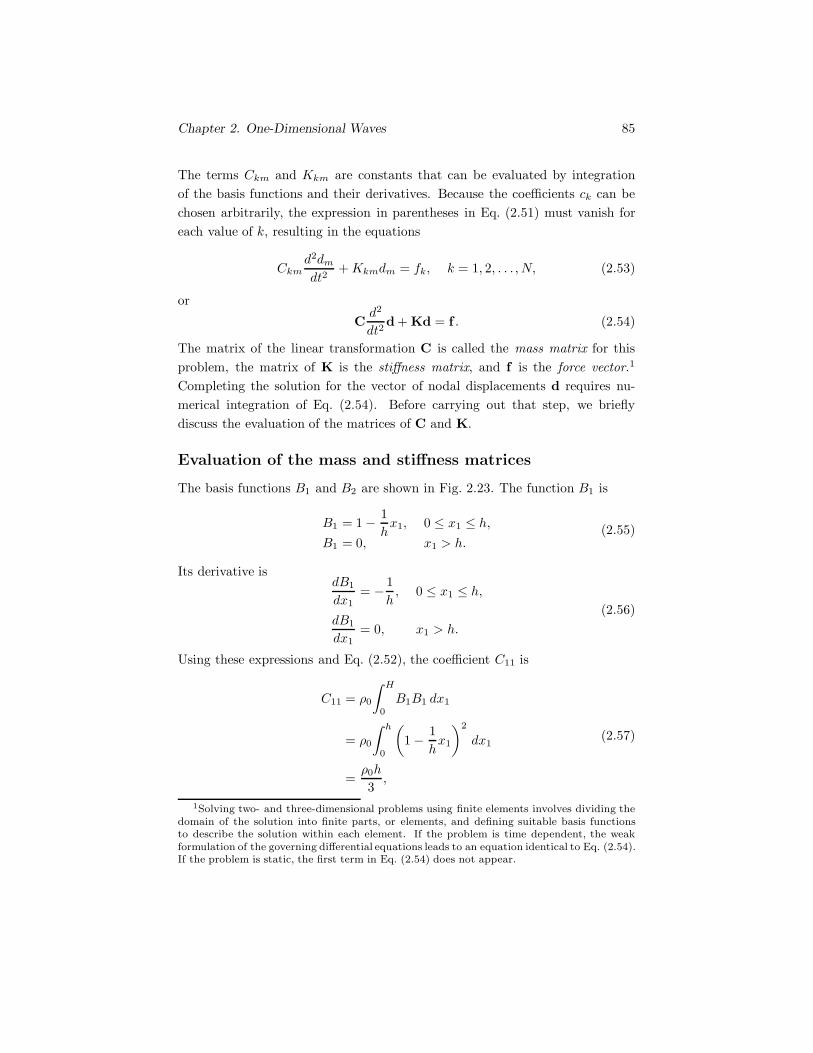
Chapter 2. One-Dimensional Waves 85
The terms Ckm and Kkm are constants that can be evaluated by integrationof the basis functions and their derivatives. Because the coefficients ck can bechosen arbitrarily, the expression in parentheses in Eq. (2.51) must vanish foreach value of k, resulting in the equations
Ckmd2dm
dt2+Kkmdm = fk, k = 1, 2, . . . , N, (2.53)
or
Cd2
dt2d + Kd = f . (2.54)
The matrix of the linear transformation C is called the mass matrix for thisproblem, the matrix of K is the stiffness matrix, and f is the force vector.1
Completing the solution for the vector of nodal displacements d requires nu-merical integration of Eq. (2.54). Before carrying out that step, we brieflydiscuss the evaluation of the matrices of C and K.
Evaluation of the mass and stiffness matrices
The basis functions B1 and B2 are shown in Fig. 2.23. The function B1 is
B1 = 1 − 1hx1, 0 ≤ x1 ≤ h,
B1 = 0, x1 > h.(2.55)
Its derivative isdB1
dx1= − 1
h, 0 ≤ x1 ≤ h,
dB1
dx1= 0, x1 > h.
(2.56)
Using these expressions and Eq. (2.52), the coefficient C11 is
C11 = ρ0
∫ H
0
B1B1 dx1
= ρ0
∫ h
0
(1 − 1
hx1
)2
dx1
=ρ0h
3,
(2.57)
1Solving two- and three-dimensional problems using finite elements involves dividing thedomain of the solution into finite parts, or elements, and defining suitable basis functionsto describe the solution within each element. If the problem is time dependent, the weakformulation of the governing differential equations leads to an equation identical to Eq. (2.54).If the problem is static, the first term in Eq. (2.54) does not appear.

Chapter 2. One-Dimensional Waves 86
x1
x1
1
1
B1
0 h 2h 3h 4h
((((((
B2
0 h 2h 3h 4h������((
((((
Figure 2.23: The basis functions B1 and B2.
and the coefficient K11 is
K11 = (λ + 2μ)∫ H
0
dB1
dx1
dB1
dx1dx1
= (λ + 2μ)∫ h
0
(− 1h
)2
dx1
=λ + 2μh
.
(2.58)
The basis function B2 is
B2 =1hx1, 0 ≤ x1 ≤ h,
B2 = 2 − 1hx1, h < x1 ≤ 2h,
B2 = 0, 2h < x1.
(2.59)

Chapter 2. One-Dimensional Waves 87
Its derivative isdB2
dx1=
1h, 0 ≤ x1 ≤ h,
dB2
dx1= − 1
h, h < x1 ≤ 2h,
dB2
dx1= 0, 2h < x1.
(2.60)
Using these expressions, the coefficient C22 is
C22 = ρ0
∫ H
0
B2B2 dx1
= ρ0
∫ h
0
(1hx1
)2
dx1 + ρ0
∫ 2h
h
(2 − 1
hx1
)2
dx1
=2ρ0h
3,
(2.61)
and the coefficient K22 is
K22 = (λ + 2μ)∫ H
0
dB2
dx1
dB2
dx1dx1
= (λ + 2μ)
[∫ h
0
(1h
)2
dx1 +∫ 2h
h
(− 1h
)2
dx1
]
=2(λ+ 2μ)
h.
(2.62)
The coefficients C12 = C21 and K12 = K21 are
C12 = ρ0
∫ H
0
B1B2 dx1
= ρ0
∫ h
0
(1 − 1
hx1
)(1hx1
)dx1
=ρ0h
6,
(2.63)
K12 = (λ + 2μ)∫ H
0
dB1
dx1
dB2
dx1dx1
= (λ + 2μ)∫ h
0
(− 1h
)(1h
)dx1
= −λ + 2μh
.
(2.64)
All of the coefficients Ckm and Kkm are determined by similar calculations.The task is greatly simplified by the repetitive nature of the basis functions.

Chapter 2. One-Dimensional Waves 88
For example, if N = 4,
Ckm = ρ0h
⎡⎢⎢⎢⎢⎢⎣
13
16
0 016
23
16 0
0 16
23
16
0 0 16
23
⎤⎥⎥⎥⎥⎥⎦ , (2.65)
Kkm =λ+ 2μh
⎡⎢⎢⎢⎣
1 −1 0 0−1 2 −1 00 −1 2 −10 0 −1 2
⎤⎥⎥⎥⎦ , (2.66)
fk = −p(t)
⎡⎢⎢⎣
1000
⎤⎥⎥⎦ . (2.67)
Numerical integration with respect to time
We now address the problem of integrating Eq. (2.54):
Cd2
dt2d + Kd = f . (2.68)
Let the velocities and accelerations of the material at the nodes be denoted by
v =d
dtd,
a =d2
dt2d =
d
dtv.
(2.69)
Equation (2.68) can be solved for the accelerations in terms of the displacements:
a = C−1 (−Kd + f ) . (2.70)
Let v(t) denote the nodal velocities at time t. If v(t) is known, the “trapezoidal”method of approximating the velocities at time t + Δt is
v(t+ Δt) = v(t) +Δt2
[a(t+ Δt) + a(t)
]. (2.71)
That is, the change in the velocity is calculated using the average accelerationduring the interval of time Δt. Then the change in the nodal displacements canbe determined in the same way using the average velocity:
d(t+ Δt) = d(t) +Δt2
[v(t+ Δt) + v(t)
]. (2.72)

Chapter 2. One-Dimensional Waves 89
However, Eqs. (2.71) and (2.72) cannot be solved sequentially, because a de-pends on d. From Eq. (2.70),
a(t) = C−1[−Kd(t) + f (t)
],
a(t + Δt) = C−1[−Kd(t+ Δt) + f (t+ Δt)
].
(2.73)
We substitute these expressions into Eq. (2.71):
v(t+ Δt) = v(t) +Δt2
C−1{−K
[d(t+ Δt) + d(t)
]+f (t+ Δt) + f (t)
}.
(2.74)
Substituting this expression for v(t+Δt) into Eq. (2.72) and solving the resultingequation for d(t+ Δt) yields
d(t+ Δt) = R−1{Sd(t) + Δtv(t)
+(Δt
2
)2
C−1[f (t+ Δt) + f (t)
]},
(2.75)
whereR = I +
(Δt2
)2
C−1K, S = I −(Δt
2
)2
C−1K, (2.76)
and I is the identity transformation, Ikm = δkm. Equation (2.75) determinesd(t+Δt) using information known at time t. (The force vector f is a prescribedfunction of time.) Once d(t + Δt) has been determined, v(t + Δt) is givenby Eq. (2.74). In this way the time evolution of the nodal displacements andvelocities can be determined iteratively. The slope of the displacement in eachelement, and therefore the stress, can be calculated using the nodal displace-ments.
Example
Let the width of the layer be H = 4. Let the density of the material be ρ = 1and let λ+ 2μ = 1, so that the wave velocity α = 1. Suppose that at t = 0, theleft side of the stationary layer is subjected to a pulse of compressive stress ofunit duration:
T11(0, t) ={
− sinπt, 0 ≤ t ≤ 1,0, 1 < t.
(2.77)
This pulse is shown in Fig. 2.24. The exact solution for the displacement field
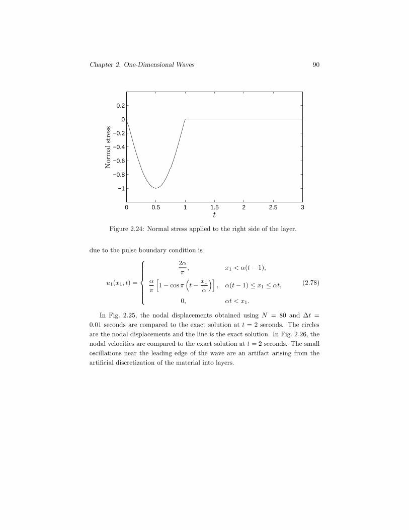
Chapter 2. One-Dimensional Waves 90
0 0.5 1 1.5 2 2.5 3
−1
−0.8
−0.6
−0.4
−0.2
0
0.2
t
Normal
stress
Figure 2.24: Normal stress applied to the right side of the layer.
due to the pulse boundary condition is
u1(x1, t) =
⎧⎪⎪⎪⎪⎪⎨⎪⎪⎪⎪⎪⎩
2απ, x1 < α(t− 1),
α
π
[1 − cosπ
(t− x1
α
)], α(t− 1) ≤ x1 ≤ αt,
0, αt < x1.
(2.78)
In Fig. 2.25, the nodal displacements obtained using N = 80 and Δt =0.01 seconds are compared to the exact solution at t = 2 seconds. The circlesare the nodal displacements and the line is the exact solution. In Fig. 2.26, thenodal velocities are compared to the exact solution at t = 2 seconds. The smalloscillations near the leading edge of the wave are an artifact arising from theartificial discretization of the material into layers.
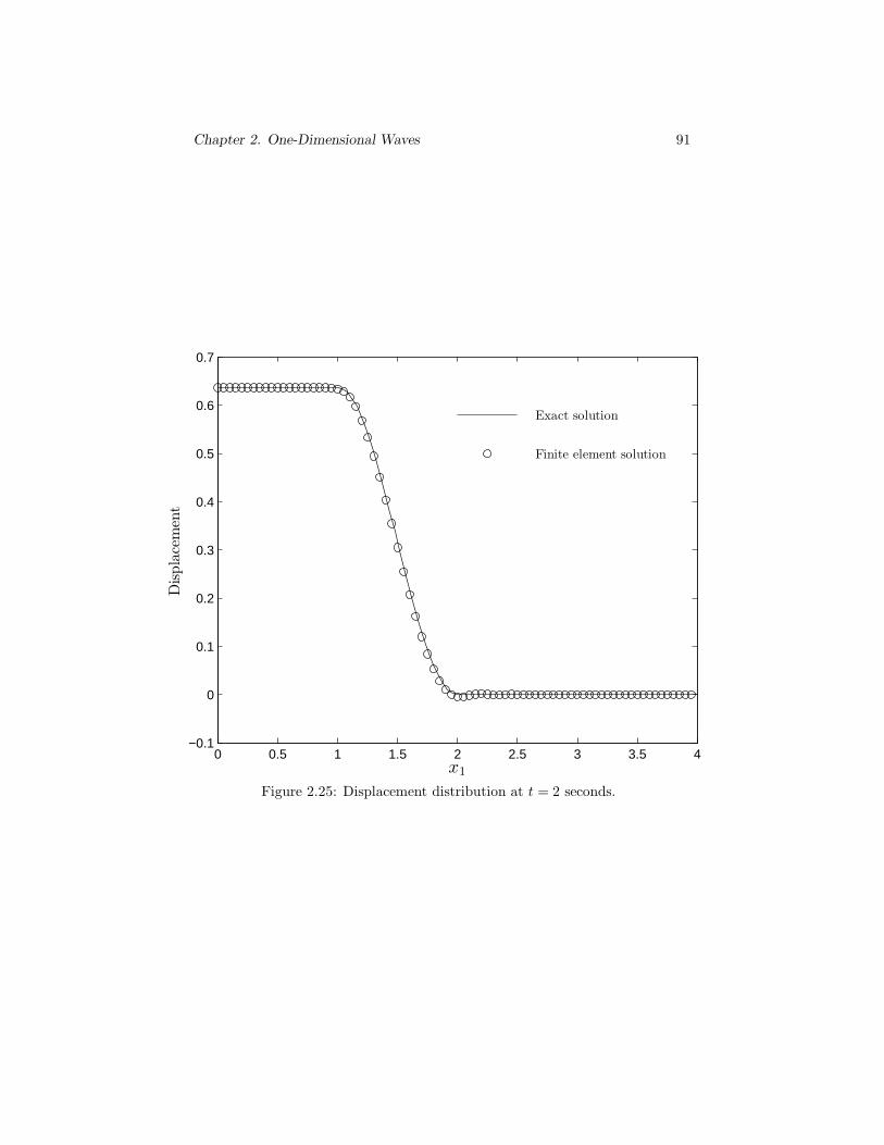
Chapter 2. One-Dimensional Waves 91
0 0.5 1 1.5 2 2.5 3 3.5 4−0.1
0
0.1
0.2
0.3
0.4
0.5
0.6
0.7
x1
Displacement
Exact solution
Finite element solution
Figure 2.25: Displacement distribution at t = 2 seconds.

Chapter 2. One-Dimensional Waves 92
0 0.5 1 1.5 2 2.5 3 3.5 4−0.2
0
0.2
0.4
0.6
0.8
1
1.2
x1
Velocity Exact solution
Finite element solution
Figure 2.26: Velocity distribution at t = 2 seconds.

Chapter 2. One-Dimensional Waves 93
2.6 Method of Characteristics
Our objective is to define the characteristics of the one-dimensional wave equa-tion and show how they can be used to obtain solutions. This approach iswidely used in solving practical one-dimensional wave problems and also helpsto explain the boundary and initial conditions that must be prescribed in suchproblems.
The one-dimensional wave equation is
∂2u
∂t2= α2∂
2u
∂x21
. (2.79)
By introducing the notation
v =∂u
∂t, ε =
∂u
∂x1,
we can write Eq. (2.79) as a first-order equation:
∂v
∂t= α2 ∂ε
∂x1. (2.80)
Because the variables v and ε are related by
∂v
∂x1=∂ε
∂t, (2.81)
we obtain a system of two first-order equations, Eqs. (2.80) and (2.81), in placeof the second-order wave equation. When u represents the displacement of anelastic material, v is the velocity of the material and ε is the strain. When u
represents the lateral displacement of a stretched string, v is the lateral velocityof the string and ε is the slope.
Let us assume that v(x1, t) and ε(x1, t) are solutions of Eqs. (2.80) and (2.81)in some region of the x1-t plane. Our objective is to show that there are lineswithin that region along which the quantity v − αε is constant. The change inthe quantity v − αε from the point x1, t to the point x1 + dx1, t+ dt is
d(v − αε) =∂
∂t(v − αε) dt+
∂
∂x1(v − αε) dx1
=(∂v
∂t− α
∂ε
∂t
)dt+
(∂v
∂x1− α
∂ε
∂x1
)dx1.
By using Eqs. (2.80) and (2.81), we can write this expression in the form
d(v − αε) =(∂v
∂x1− 1α
∂v
∂t
)(dx1 − α dt) .

Chapter 2. One-Dimensional Waves 94
From this equation, d(v − αε) is zero if
dx1
dt= α.
That is, the quantity v−αε is constant along any straight line in the x1-t planehaving slope α. In the same way, it can be shown that the quantity v + αε isconstant along any straight line in the x1-t plane having slope
dx1
dt= −α.
Straight lines in the x1-t plane having slopes α and −α are called character-istics of the one-dimensional wave equation. When the x1-t plane is representedas shown in Fig. 2.27, we refer to the two types as right-running and left-runningcharacteristics. The quantity v−αε is constant along a right-running character-istic, and the quantity v+αε is constant along a left-running characteristic. Inthe following sections we show that these two conditions can be used to obtainsolutions to Eqs. (2.80) and (2.81).
x1
t
left-running right-running
1 1α α)))))
*****
Figure 2.27: Left- and right-running characteristics in the x1-t plane.
Initial-value problem
Suppose that at t = 0, the velocity and strain of an unbounded elastic materialare prescribed:
v(x1, 0) =∂u1
∂t(x1, 0) = p(x1),
ε(x1, 0) =∂u1
∂x1(x1, 0) = q(x1),
where p(x1) and q(x1) are given functions. We assume that the velocities anddisplacements of the material in the x2 and x3 directions are zero at t = 0. Wecan use characteristics to determine the velocity and strain of the material asfunctions of position and time.
Consider an arbitrary point x1, t in the x1-t plane. We can extend a right-running characteristic ab and a left-running characteristic ac from this point

Chapter 2. One-Dimensional Waves 95
back to the x1 axis (Fig. 2.28). They intersect the x1 axis at x1 − αt and atx1+αt respectively. Along the right-running characteristic ab, v−αε is constant:
x1 − αt x1 + αt
x1, ta
b cx1
t
******
))))))
� �
�
Figure 2.28: Characteristics for the initial-value problem.
v(x1 , t)− αε(x1, t) = p(x1 − αt) − αq(x1 − αt).
Along the left-running characteristic ac, v + αε is constant:
v(x1 , t) + αε(x1, t) = p(x1 + αt) + αq(x1 + αt).
We can solve these two equations for v(x1, t) and ε(x1, t):
v(x1, t) =12[p(x1 + αt) + p(x1 − αt)] +
α
2[q(x1 + αt) − q(x1 − αt)],
ε(x1, t) =12α
[p(x1 + αt) − p(x1 − αt)] +12[q(x1 + αt) + q(x1 − αt)].
Thus we have determined the velocity and strain fields in the material in termsof the initial velocity and strain distributions.
Initial-boundary value problem
Suppose that a half space of elastic material is initially undisturbed, and att = 0 we subject the boundary to the velocity boundary condition
v(0, t) =∂u1
∂t(0, t) = p(t), (2.82)
where p(t) is a prescribed function of time that vanishes for t < 0 (Fig. 2.29).Consider an arbitrary point x1, t in the x1-t plane. We can extend a left-
running characteristic ab from this point back to the x1 axis (Fig. 2.30). Becausethe material is undisturbed at t = 0, the velocity v = 0 and the strain ε = 0at each point on the x1 axis. Along the left-running characteristic ab, v + αε isconstant. Therefore
v(x1, t) + αε(x1, t) = 0. (2.83)

Chapter 2. One-Dimensional Waves 96
x1
v(0, t) =∂u1
∂t(0, t) = p(t)
�������
Figure 2.29: Half space subjected to a velocity boundary condition.
x1, t
t− x1
α
a
c
d bx1
t
))))*******
)))))))))))
�
�
�
�
Figure 2.30: Characteristics for a velocity boundary condition.
We can also extend a right-running characteristic ac from the point x1, t back tothe t axis. As indicated in the figure, it intersects the t axis at t− x1/α. Alongthe right-running characteristic ac, v − αε is constant. However, although weknow the velocity v at point c because the velocity is prescribed as a functionof time at x1 = 0, we do not know the strain at point c. To determine it, wecan extend a left-running characteristic from point c back to the x1 axis. Fromthe characteristic cd we obtain the relation
v(0, t− x1
α
)+ αε
(0, t− x1
α
)= 0. (2.84)
Thus the value of the strain at point c is
ε(0, t− x1
α
)= − 1
αv(0, t− x1
α
)= − 1
αp(t− x1
α
),
where we have used Eq. (2.82). Now that the strain at point c is known, theright-running characteristic ac gives the relation
v(x1, t) − αε(x1, t) = v(0, t− x1
α
)− αε
(0, t− x1
α
)

Chapter 2. One-Dimensional Waves 97
= 2p(t − x1
α
).
We can solve this equation and Eq. (2.83) for v(x1, t) and ε(x1, t) in terms ofthe prescribed boundary condition:
v(x1, t) = p(t− x1
α
),
ε(x1, t) = − 1αp(t− x1
α
).
These results show that the solution has a remarkably simple structure: thevelocity v and the strain ε are constant along right-running characteristics.
On page 95, we considered initial-boundary value problems in a half spaceand assumed that either the displacement or the stress was prescribed at theboundary. Our discussion in this section explains why both the displacementand the stress are not prescribed in such problems. Prescribing the displacementimplies that the velocity is prescribed, and prescribing the stress is equivalentto prescribing the strain. Equation (2.84), which we obtained from the charac-teristic cd, shows that the values of the velocity and the strain at the boundaryare not independent, but are related through the initial condition. As a result,it is possible to prescribe either the velocity or the strain at the boundary, butnot both.
Exercises
Exercise 2.14 By using Eqs. (2.80) and (2.81), show that the quantity v+αε
is constant along any straight line in the x-t plane having slope
dx
dt= −α.
Exercise 2.15
x1
T11(0, t) = p(t)
�������

Chapter 2. One-Dimensional Waves 98
Suppose that a half space of elastic material is initially undisturbed, and att = 0 the boundary is subjected to the stress boundary condition
T11(0, t) = p(t),
where p(t) is a prescribed function of time that vanishes for t < 0. Use themethod of characteristics to determine the velocity and strain of the materialat an arbitrary point x1, t in the x1-t plane.
Answer:v(x1 , t) = − α
λ+ 2μp(t− x1
α
),
ε(x1, t) =1
λ+ 2μp(t− x1
α
).
Exercise 2.16
zL zR
v0 v0� �
Half spaces of materials with acoustic impedances zL = ρLαL and zR = ρRαR
approach each other with equal velocities v0. Use characteristics to show thatthe velocity of their interface after the collision is v0(zL − zR)/(zL + zR).
Exercise 2.17 Consider the first-order partial differential equation
∂u
∂t+ α
∂u
∂x= 0,
where α is a constant. Show that its solution u(x, t) is constant along charac-teristics with slope dx/dt = α.

Chapter 2. One-Dimensional Waves 99
2.7 Waves in Layered Media
In the previous section we used the method of characteristics to analyze one-dimensional waves in a plate, or layer, of elastic material. The same approachworks for waves in several bonded layers (Fig. 2.31), although it is tediousbecause of the number of equations involved. In this section we describe twoprocedures that efficiently analyze waves in a particular class of layered elasticmedia.
x1
Figure 2.31: Bonded layers of elastic materials.
Along right-running characteristics within each layer,
v − αε = constant, (2.85)
and along left-running characteristics,
v + αε = constant. (2.86)
The product of the acoustic impedance z = ρ0α and the term αε is
zαε = ρ0α2∂u1
∂x1= (λ + 2μ)
∂u1
∂x1= T11.
In the following development we denote the component of normal stress T11
by σ. Multiplying Eqs. (2.85) and (2.86) by z yields the relations
zv − σ = constant (2.87)
along right-running characteristics and
zv + σ = constant (2.88)
along left-running characteristics. This transformation of the equations is conve-nient because, while the strain ε is not continuous across the interfaces betweenlayers, both the velocity v and normal stress σ are.

Chapter 2. One-Dimensional Waves 100
Define new independent variables n and j by
t = Δj, (2.89)
dx1 = αΔn, (2.90)
where Δ is a time interval. Consider a finite number of bonded layers with theleft boundary of the first layer at n = 0 and the right boundary of the last layerat n = L, where L is an integer. We assume that the time interval Δ can bechosen so that interfaces between layers occur only at integer values of n.
First algorithm
As a consequence of Eqs. (2.89) and (2.90), left-running and right-running char-acteristics join points defined by integer values of j and n (Fig. 2.32). The
t/Δ
x1/αΔ
layer interface
left-runningcharacteristic
right-runningcharacteristic
n− 1 n n+ 1
j − 1
j
j + 1
��
��
���
�����
�����
........................................................................................................................................................................................................................
........................................................................................................................................................................................................................
........................................................................................................................................................................................................................
......
......
......
......
......
......
......
......
......
......
......
......
......
......
......
......
......
......
......
......
......
......
......
......
......
......
......
......
.....
......
......
......
......
......
......
......
......
......
......
......
......
......
......
......
......
......
......
......
......
......
......
......
......
......
......
......
......
.....
......
......
......
......
......
......
......
......
......
......
......
......
......
......
......
......
......
......
......
......
......
......
......
......
......
......
......
......
.....
�����
$$$$$
$$$
$$
���
��
Figure 2.32: Points corresponding to integer values of j and n.
methods we describe evaluate the dependent variables v(n, j) and σ(n, j) onlyat these points. However, that does not mean that solutions can be obtainedonly at boundaries of layers. By dividing an individual layer into several sub-layers, solutions can be determined at points within a layer.
For a given position n, we denote the acoustic impedances to the left andright by z(n)− and z(n)+, respectively. Notice that z(n)− = z(n − 1)+. Wealso define
z(n) = 12 [z(n)+ + z(n)−]. (2.91)
With Eqs. (2.87) and (2.88), we can establish relationships between the valuesof v and σ at the points shown in Fig. 2.32. From the two characteristics at the

Chapter 2. One-Dimensional Waves 101
top of the “diamond,” we obtain
z(n)−v(n, j + 1) − σ(n, j + 1) = z(n)−v(n − 1, j) − σ(n − 1, j) (2.92)
and
z(n)+v(n, j + 1) + σ(n, j + 1) = z(n)+v(n + 1, j) + σ(n + 1, j). (2.93)
Addition of these two equations yields
2z(n)v(n, j + 1) = z(n)+v(n + 1, j) + z(n)−v(n − 1, j)
+ σ(n+ 1, j) − σ(n − 1, j).(2.94)
We can use Eqs. (2.92) and (2.94) to analyze initial-boundary value problemsin the layered medium. Initial conditions σ(n, 0) and v(n, 0) must be specified.Then Eq. (2.94) determines v(n, 1) and Eq. (2.92) determines σ(n, 1). Thesecalculations can be carried out in any order for all values of n except n = 0and n = L. At the left boundary, n = 0, Eq. (2.93) must be used, and eitherv(0, 1) or σ(0, 1) must be specified. Similarly, at the right boundary, n = L,Eq. (2.92) must be used, and either v(L, 1) or σ(L, 1) must be specified. Thisprocess can be repeated for successive values of j until a prescribed final timeis reached.
Each application of Eqs. (2.92) and (2.94) requires nine arithmetic opera-tions. In the next section we describe an alternative algorithm that determinesonly the velocity, but is simpler and more efficient, both for computing simpleexamples by hand and for solving problems involving many layers by computer.
Second algorithm
In this method we employ four relations: Eqs. (2.92) and (2.93), together withthe two characteristic relations obtained from the bottom of the diamond inFig. 2.32,
z(n)−v(n, j − 1) + σ(n, j − 1) = z(n)−v(n − 1, j) + σ(n − 1, j) (2.95)
and
z(n)+v(n, j − 1) − σ(n, j − 1) = z(n)+v(n + 1, j) − σ(n + 1, j). (2.96)
Addition of these four relations yields the new algorithm:
z(n)[v(n, j + 1) + v(n, j − 1)] = z(n)+v(n + 1, j) + z(n)−v(n − 1, j). (2.97)

Chapter 2. One-Dimensional Waves 102
This equation determines v(n, j+1) with only four arithmetic operations. Whenthe acoustic impedance is continuous at n, z(n) = z(n)+ = z(n)−, it furthersimplifies to
v(n, j + 1) + v(n, j − 1) = v(n + 1, j) + v(n − 1, j). (2.98)
The sequence of calculations using Eq. (2.97) is roughly the same as for thefirst algorithm, but because σ does not appear explicitly, the initial and bound-ary conditions are handled somewhat differently. The initial conditions σ(n, 0)and v(n, 0) must be specified as before. Then Eq. (2.94) determines v(n, 1), andfrom that point onward, Eq. (2.97) determines v. When σ is specified at theleft boundary, Eqs. (2.93) and (2.96) are evaluated for n = 0 and summed toobtain
v(0, j + 1) + v(0, j − 1) = 2v(1, j) − 1z(0)+
[σ(0, j + 1) − σ(0, j − 1)], (2.99)
and when σ is specified at the right boundary,
v(L, j+1)+v(L, j−1) = 2v(L−1, j)+1
z(L)−[σ(L, j+1)−σ(L, j−1)]. (2.100)
These two algorithms have an interesting property. The values of σ and v atpoints where j+n is even are determined by the boundary and initial conditionsat points where j+n is even, and the values of σ and v at points where j+n isodd are determined by the boundary and initial conditions at points where j+nis odd. This is most apparent in Eq. (2.98). We can compute either the even orodd solution independently, requiring one-half the number of computations.
Examples
1. A single layer Consider a layer of an elastic material that is initiallyundisturbed, and suppose that for t > 0 the left boundary is subjected to a unitstep in velocity, v(0, t) = 1. Let the right boundary be fixed. We divide thelayer into 5 sublayers to determine the solution, so that in terms of n and j, theboundary conditions are v(0, j) = 1 and v(5, j) = 0.
Using Eq. (2.98) to obtain the odd solution, we obtain the results in Fig. 2.33.The numbers in the figure are the values of the velocity corresponding to theindicated values of n and j. The three zero values of the solution for j = 0 comefrom the initial conditions. The next row of values, at j = 1, is determined bythe left boundary condition v(0, 1) = 1 and Eq. (2.94), which reduces to
2v(n, 1) = v(n + 1, 0) + v(n − 1, 0).

Chapter 2. One-Dimensional Waves 103
n
j
v(0, j) = 1︸ ︷︷ ︸ v(5, j) = 0︸ ︷︷ ︸
{v(n, 0) = σ(n, 0) = 0
0 1 2 3 4 50123456789
1
1
1
1
1
1
1
1
1
1
1
1
1
11
0
0
0
0
0
0
0
0
0
0
0
0
0
0
0
Figure 2.33: A layer with a specified velocity at the left boundary and fixed atthe right boundary.
(Because σ(n, 0) = 0 and z(n) = z(n)+ = z(n)−, the solution does not dependon the acoustic impedance.)
The next row of values is obtained using the right boundary condition andEq. (2.98),
v(n, 2) = v(n + 1, 1) + v(n − 1, 1)− v(n, 0).
The remaining rows are determined by repeated applications of Eq. (2.98). Ahand calculation of this part of the solution is simplified by visualizing eachsolution point as the top of the diamond in Fig. 2.32 and noticing from Eq. (2.98)that the sum of values at the top and bottom of the diamond equals the sum ofthe values on the left and right sides.
Figure 2.33 shows the wave initiated at the left boundary at j = 0 propa-gating at velocity α, advancing one integer value of n for each integer increasein j. Behind the wave front, the velocity equals the constant velocity at the leftboundary. When the wave reaches the fixed right boundary, a reflected wavepropagates back toward the left boundary. The velocity behind the reflectedwave is zero.
If the right boundary of the plate is free instead of fixed, the only differencein the computation is that we use Eq. (2.100),
v(5, j + 1) = 2v(4, j) − v(5, j − 1),
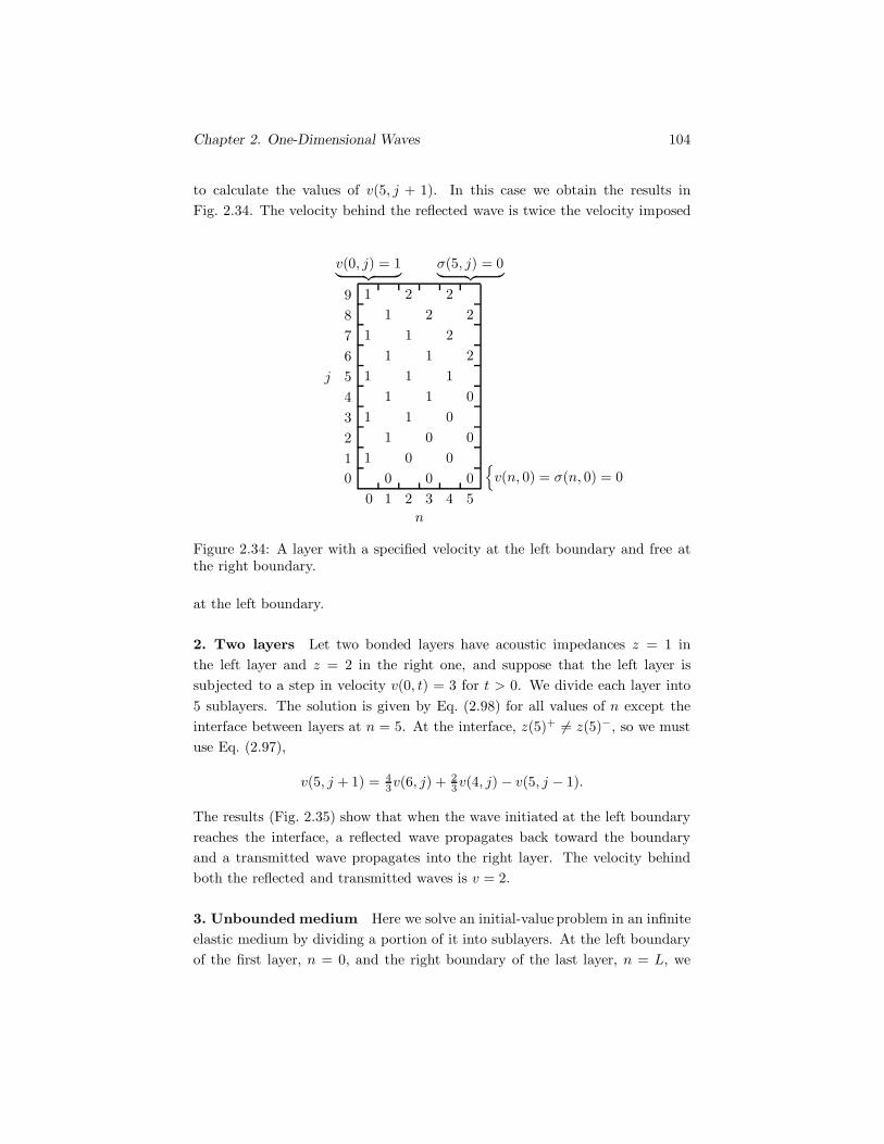
Chapter 2. One-Dimensional Waves 104
to calculate the values of v(5, j + 1). In this case we obtain the results inFig. 2.34. The velocity behind the reflected wave is twice the velocity imposed
n
j
v(0, j) = 1︸ ︷︷ ︸ σ(5, j) = 0︸ ︷︷ ︸
{v(n, 0) = σ(n, 0) = 0
0 1 2 3 4 50123456789
1
1
1
1
1
1
1
1
1
1
1
1
1
11
0
0
0
0
0
0
00
0
2
22
22
2
Figure 2.34: A layer with a specified velocity at the left boundary and free atthe right boundary.
at the left boundary.
2. Two layers Let two bonded layers have acoustic impedances z = 1 inthe left layer and z = 2 in the right one, and suppose that the left layer issubjected to a step in velocity v(0, t) = 3 for t > 0. We divide each layer into5 sublayers. The solution is given by Eq. (2.98) for all values of n except theinterface between layers at n = 5. At the interface, z(5)+ �= z(5)−, so we mustuse Eq. (2.97),
v(5, j + 1) = 43v(6, j) + 2
3v(4, j) − v(5, j − 1).
The results (Fig. 2.35) show that when the wave initiated at the left boundaryreaches the interface, a reflected wave propagates back toward the boundaryand a transmitted wave propagates into the right layer. The velocity behindboth the reflected and transmitted waves is v = 2.
3. Unbounded medium Here we solve an initial-value problem in an infiniteelastic medium by dividing a portion of it into sublayers. At the left boundaryof the first layer, n = 0, and the right boundary of the last layer, n = L, we

Chapter 2. One-Dimensional Waves 105
n
j
v(0, j) = 3︸ ︷︷ ︸ v(10, j) = 0︸ ︷︷ ︸
{v(n, 0) = σ(n, 0) = 0
z = 1 z = 2� �� �
0 1 2 3 4 5 6 7 8 9 100123456789
10
3
3
3
3
3
3
3
3
3
3
3
3
3
33
0
0
0
0
0
0
0
0
0
0
0
0
0
0
0
0
0
0
0
0
0
0
0
0
0
0
0
00
0
22
2
2
2
2
2
2
2
2
22
22
2
Figure 2.35: Two layers with a specified velocity at the left boundary.
impose conditions that prevent reflections of waves and thus simulate an infinitemedium. The D’Alembert solution for a right-traveling wave is
u1 = f(ξ),
where ξ = x1 − αt. The velocity and normal stress are
v = −αdfdξ, σ = (λ + 2μ)
df
dξ,
so in a right-traveling wave, v and σ are constant along characteristics ξ =constant. Equations (2.89) and (2.90) imply that within a sublayer, ξ is constantwhen n− j is constant. Because
n− (j + 1) = (n − 1) − j,
reflected waves are prevented at the right boundary, n = L, if we impose theconditions
v(L, j + 1) = v(L − 1, j),σ(L, j + 1) = σ(L − 1, j).
By similar arguments, reflected waves are prevented at the left boundary, n = 0,if we impose the conditions
v(0, j + 1) = v(1, j), (2.101)
σ(0, j + 1) = σ(1, j). (2.102)

Chapter 2. One-Dimensional Waves 106
We assume that at t = 0 the strain is zero and the velocity is zero except in afinite region in which v(x, 0) = 2 (Fig. 2.36). The solution is given by Eqs. (2.94)and (2.98) together with the conditions imposed at the boundaries. The results
n
j
v(0, j + 1) = v(1, j)︸ ︷︷ ︸ v(10, j + 1) = v(9, j)︸ ︷︷ ︸
{σ(n, 0) = 0v(n, 0) = F (n)
0 1 2 3 4 5 6 7 8 9 100123456
00
00
0
00
0
00
1
1
1
1
1
1
1
1
1
11 1
1
1
1
1
1
1
1
1
1
1
22
2
22
2
Figure 2.36: An unbounded medium subjected to an initial velocity.
show waves propagating to the left and right within which the velocity of thematerial equals one-half of the velocity imposed at t = 0. Behind these waves,the medium is stationary. Notice that the conditions imposed at the boundariesprevent reflected waves.
4. Periodically layered medium Our first three examples illustrate wavebehavior using cases simple enough to compute by hand, but the real utility ofthese methods becomes evident when they are applied to layered media withlarge numbers of layers. As an example, we consider a medium consisting ofalternating layers of two elastic materials. One material has acoustic impedancez = 1 and consists of layers of thickness 10αΔ, and the other material hasacoustic impedance z = 200 and consists of layers of thickness αΔ.
Suppose that the left boundary of the medium is subjected to a unit step invelocity, v(0, t) = 1, for t > 0. We evaluate the odd solution from Eq. (2.97) byusing the following program:
• Initialize storage:
• z is a vector with 1101 elements initialized to 1. v is a matrix with(1101, 1501) elements initialized to 0. Subscripts start at 0.
• for (n = 11 to 1100 by increments of 11) z(n) = 200.

Chapter 2. One-Dimensional Waves 107
• Using Eq. (2.91), compute z(n)+
z(n) and z(n)−
z(n) :
• for (n = 1 to 1099 by increments of 1) begin
– zp(n) = 2 ∗ z(n+ 1)/(z(n) + z(n+ 1))
– zm(n) = 2 ∗ z(n)/(z(n) + z(n+ 1))
• end for
• Specify left boundary condition:
• for (j = 1 to 1499 by increments of 2) v(0, j) = 1.
• Start time loop to compute solution:
• for (j = 1 to 1499 by increments of 1) begin
– if j is even ns = 2 else ns = 1
– Using Eq. (2.97), compute odd solution—exclude right boundary:
– for (n = ns to 1099 by increments of 2) v(n, j + 1) =zp(n) ∗ v(n + 1, j) + zm(n) ∗ v(n − 1, j) − v(n, j − 1)
• end for
The computer’s memory must be large enough to hold the values of v forall values of n and j simultaneously, including the values of the even solutionthat remain as zeros. To simplify the program, we used only Eq. (2.97), eventhough Eq. (2.98) is more efficient at interfaces between sublayers where zp(n) =zm(n) = 1.
The computed velocity at the center of the thirty-first layer (n=170) is shownas a function of j (nondimensional time) in Fig. 2.37. As a result of the mul-tiple reflections and transmissions at the layer interfaces, the velocity has anoscillatory history. This oscillatory profile is seen in sound propagation throughducts, elastic waves in channels and bars, and ocean tidal surges, or bores, intorivers and channels, and is called an undulating bore. This behavior results froma phenomenon known as dispersion, which we discuss in the next chapter.

Chapter 2. One-Dimensional Waves 108
v
j/1000
0.0
0.5
1.0
1.5
0.5 1.0 1.5
Figure 2.37: Velocity at a point in a periodically layered medium resulting froma unit step in velocity at the boundary.

Chapter 2. One-Dimensional Waves 109
Exercises
Exercise 2.18 Use D’Alembert solutions to verify the values shown in Fig. 2.34.
Exercise 2.19
(a) Use Eq. (2.98) to verify the values shown in Fig. 2.34.(b) Extend the calculation shown in Fig. 2.34 to j = 15.
Exercise 2.20 Extend the calculations used to obtain Fig. 2.34 to j = 15,assuming that at t = 0 the left boundary is subjected to a unit step in stress,σ(0, t) = 1.
Exercise 2.21 Repeat the calculations used to obtain Fig. 2.33, replacing theunit step in velocity at the left boundary by the pulse
v(0, j) ={
1 j = 0,0 j > 0.
Exercise 2.22 Calculate the results shown in Fig. 2.37.

Chapter 3
Steady-State Waves
Steady-state waves are waves in which the dependent variablesare harmonic, or oscillatory functions of time. Waves that are notsteady-state are said to be transient. Most of the waves we en-counter, both natural and man-made, are transient. We study steady-state waves for the insights they provide and because, at least con-ceptually, transient wave solutions can be obtained by superimposingsteady-state solutions. Furthermore, with modern ultrasonic devicesit is possible to create steady-state waves.
We begin by discussing one-dimensional steady-state waves, thenderive representations of steady-state compressional and shear wavesin two dimensions. Using these representations, we obtain solutionsfor the reflection of plane waves at a free boundary, Rayleigh waves,waves in a layer of elastic material, and waves in layered media.
3.1 Steady-State One-Dimensional Waves
We will first show that the one-dimensional wave equation admits a solutionthat has a harmonic dependence on time. We then introduce the terminol-ogy of steady-state waves and consider some one-dimensional problems havingharmonic boundary conditions.
Consider the one-dimensional wave equation
∂2u
∂t2= α2∂
2u
∂x2. (3.1)
Let us seek a solution of this equation that is a harmonic, or oscillatory functionof time:
u = f(x) sin ωt, (3.2)
110

Chapter 3. Steady-State Waves 111
where ω is a constant and f(x) is a function that must be determined. Sub-stituting this expression into Eq. (3.1) shows that Eq. (3.1) is satisfied if thefunction f(x) is a solution of the equation
d2f(x)dx2
+ω2
α2f(x) = 0.
The general solution of this ordinary differential equation can be expressed inthe form
f(x) = 2A sinω
αx+ 2B cos
ω
αx,
where A and B are arbitrary constants. Substituting this expression intoEq. (3.2), we obtain a solution of the one-dimensional wave equation:
u = 2A sinω
αx sinωt + 2B cos
ω
αx sinωt.
We can write this equation in the form
u = A[cosω
( xα− t
)− cosω
(xα
+ t)]
−B[sinω
(xα− t
)− sinω
(xα
+ t)].
Observe that we have obtained D’Alembert solutions in terms of sines andcosines. Solutions of this form are called steady-state solutions. With x heldfixed, the dependent variable undergoes a steady harmonic oscillation in time.
Let us consider a wave represented by the steady-state solution
u = A cosω(xα− t
)= A cos(kx− ωt). (3.3)
The constantk =
ω
α(3.4)
is called the wave number of the steady-state solution. The absolute value ofthe constant A is called the amplitude of the wave, and the speed α is calledthe phase velocity of the wave.
Figure 3.1.a shows a graph of u as a function of x with the time t held fixed.The distance λ required for the solution to undergo a complete oscillation iscalled the wavelength of the wave. From Eq. (3.3) we see that with t heldfixed the solution undergoes one complete oscillation when kx changes by 2π.Therefore kλ = 2π, so the wave number is related to the wavelength by
k =2πλ. (3.5)
Figure 3.1.b shows a graph of u as a function of t with the position x heldfixed. The time T required for the solution to undergo one complete oscillation

Chapter 3. Steady-State Waves 112
x
u
λ
|A|
(a)
� �
�
�
t
u
T
|A|
(b)
� �
�
�
Figure 3.1: The dependent variable u: (a) as a function of x; (b) as a functionof t.
is called the period of the wave. From Eq. (3.3), we see that with x heldfixed the solution undergoes one complete oscillation when ωt changes by 2π.Therefore ωT = 2π, so the constant ω is related to the period by
ω =2πT. (3.6)
The inverse of the period f = 1/T is the number of oscillations per unit timeat a fixed position x. It is called the frequency of the wave. From Eq. (3.6), wesee that
f =1T
=ω
2π(3.7)
When the position x is held fixed, there is a one-to-one correspondencebetween the value of u and the vertical position of a point moving in a circularpath of radius |A| with constant angular velocity ω. Figure 3.2 shows thiscorrespondence for the position x = 0. The period T is the time required forthe point to move once around the circular path. The frequency f is the numberof revolutions of the point around the circular path per unit time, and ω = 2πfis the number of radians around the circular path per unit time. Thus f and ω

Chapter 3. Steady-State Waves 113
t
u
|A||A| cosωt
{ωt
�
�
����
�� � ��..........................................................................................................................
Figure 3.2: Correspondence between the dependent variable u and the motionof a point in a circular path.
are both measures of the frequency. The term f is measured in oscillationsor cycles per second, which are called Hertz (Hz). The term ω is measured inradians per second, and is sometimes called the circular frequency to distinguishit from f . From Eqs. (3.4), (3.5), and (3.7), we obtain a simple relation betweenthe phase velocity, the wavelength, and the frequency:
α = λf. (3.8)
It is often convenient to use the complex exponential function, Eq. (A.2), toexpress steady-state waves in the form
u = Aei(kx − ωt) = A[cos(kx− ωt) + i sin(kx− ωt)],
where the constant A may be complex. The magnitude of A is the amplitudeof the wave. We call A the complex amplitude of the wave.
For example, suppose that a plate of elastic material of thickness L is sub-jected to the steady-state displacement boundary condition
u1(0, t) = Ue−iωt
at the left boundary, where U is a constant, and the plate is bonded to a fixedsupport at the right boundary (Fig. 3.3). Let us determine the resulting steady-state motion of the material.
The steady-state boundary condition gives rise to a steady-state wave prop-agating in the positive x1 direction. Due to reflection at the boundary, there isalso a steady-state wave propagating in the negative x1 direction. Therefore weassume a steady-state solution of the form
u1 = Tei(kx1 − ωt) + Rei(−kx1 − ωt), (3.9)

Chapter 3. Steady-State Waves 114
x1
u1(0, t) = Ue−iωt
L
�������� �
Figure 3.3: Plate with a steady-state displacement boundary condition.
where T is the complex amplitude of the forward-propagating transmitted waveand R is the complex amplitude of the rearward-propagating reflected wave.Substituting this expression into the boundary condition at the left boundary,we obtain the equation
T +R = U.
Requiring the displacement to be zero at the right boundary yields the equation
TeikL + Re−ikL = 0.
The solution of these two equations for the values of the complex amplitudesare
T =e−ikLU
e−ikL − eikL, R =
−eikLUe−ikL − eikL
.
By using these results, we can express Eq. (3.9) in the form
u1 = −U sin[k(x1 − L)]sin kL
e−iωt.
This solution exhibits the interesting phenomenon of resonance. It predictsthat the amplitude of the displacement is infinite when sin kL = 0; that is, whenkL = nπ, where n is an integer. From Eq. (3.5), we see that this occurs whenthe wavelength satisfies the relation nλ/2 = L. That is, the width of the plateequals an integral number of half-wavelengths (Fig. 3.4).

Chapter 3. Steady-State Waves 115
n = 3
n = 2
n = 1
Figure 3.4: Resonance occurs when the width of the plate is equal to an integralnumber of half-wavelengths.

Chapter 3. Steady-State Waves 116
Exercises
Exercise 3.1 Show thatu = Aei(kx− ωt)
is a solution of Eq. (3.1) if k = ω/α.
Exercise 3.2
x1
T11(0, t) = T0e−iωt
�������
A half space of elastic material is subjected to the stress boundary condition
T11(0, t) = T0e−iωt,
where T0 is a constant. Determine the resulting steady-state displacement fieldin the material.
Answer:u1 =
T0
ik(λ + 2μ)ei(kx1 − ωt),
where k = ω/α.
Exercise 3.3
x1
u1(0, t) = Ue−iωt
L
�������� �
A plate of elastic material of thickness L is subjected to the steady-state dis-placement boundary condition
u1(0, t) = Ue−iωt

Chapter 3. Steady-State Waves 117
at the left boundary. The plate is free at the right boundary. Determine theresulting steady-state displacement field in the material.
Discussion—Assume a steady-state solution of the form
u1 = Tei(kx1 − ωt) + Rei(−kx1 − ωt),
where T and R are constants and k = ω/α.Answer:
u1 =U cos[k(x1 − L)]
cos kLe−iωt.
Exercise 3.4
x1
T12(0, t) = T0e−iωt
L
�
�
�
� �
A plate of elastic material of thickness L is subjected to the steady-state shearstress boundary condition
T12(0, t) = T0e−iωt
at the left boundary. The plate is bonded to a rigid material at the right bound-ary. Determine the resulting steady-state displacement field in the material.
Answer:
u1 =T0 sin[k(x1 − L)]
kμ cos kLe−iωt,
where k = ω/β.

Chapter 3. Steady-State Waves 118
3.2 Steady-State Two-Dimensional Waves
We will begin by obtaining “building-block” solutions that will be used in thefollowing sections to analyze several important problems in elastic wave propa-gation. Consider the elastic half space and coordinate system shown in Fig. 3.5.We assume that the motion of the material is described by the displacementfield
u1 = u1(x1, x3, t),u2 = 0,u3 = u3(x1, x3, t).
(3.10)
Thus the motion is two-dimensional: it does not depend on the coordinate
x1
x3
Figure 3.5: An elastic half space.
normal to the plane in Fig. 3.5, and the component of the displacement normalto the plane is zero. This type of motion is called plane strain. Using theHelmholtz decomposition
u = ∇φ+ ∇× ψ,
we can express the displacement components in terms of two scalar potentials:
u1 =∂φ
∂x1− ∂ψ2
∂x3,
u3 =∂φ
∂x3+∂ψ2
∂x1,
(3.11)
where φ = φ(x1, x3, t) and ψ2 = ψ2(x1, x3, t). The scalar ψ2 is the x2 componentof the vector potential ψ. To simplify the notation, we will drop the subscript 2and write the scalar ψ2 as ψ.
The potentials φ and ψ are governed by the wave equations
∂2φ
∂t2= α2
(∂2φ
∂x21
+∂2φ
∂x23
)(3.12)
and∂2ψ
∂t2= β2
(∂2ψ
∂x21
+∂2ψ
∂x23
), (3.13)

Chapter 3. Steady-State Waves 119
where the compressional and shear wave speeds α and β are defined in terms ofthe Lame constants λ and μ and the density ρ0 of the material:
α =(λ+ 2μρ0
)1/2
, β =(μ
ρ0
)1/2
.
Let us assume that the potential φ is given by the steady-state equation
φ = f(x3)ei(k1x1 − ωt), (3.14)
where the wave number k1 and the frequency ω are prescribed and the func-tion f(x3) must be determined. Thus we assume that the solution for thepotential φ has the form of a steady-state wave propagating in the positive x1
direction, but we make no assumption about the behavior of the solution inthe x3 direction. Substituting this expression into Eq. (3.12), we find that thefunction f(x3) must satisfy the ordinary differential equation
d2f(x3)dx2
3
+(ω2
α2− k2
1
)f(x3) = 0. (3.15)
The solutions of this equation result in solutions for φ that have very differentcharacters depending on whether k2
1 < ω2/α2 or k21 > ω2/α2. We discuss these
cases separately.
Plane waves propagating in the x1-x3 plane
If k21 < ω2/α2, it is convenient to write the solution of Eq. (3.15) in the form
f(x3) = Aeik3x3 +Be−ik3x3 ,
where A and B are constants and
k3 =(ω2
α2− k2
1
)1/2
.
Substituting this form of the solution for f(x3) into Eq. (3.14), we obtain thesolution for the potential φ in the form
φ = Aei(k1x1 + k3x3 − ωt) + Bei(k1x1 − k3x3 − ωt). (3.16)
Consider the first term of this solution:
φ = Aei(k1x1 + k3x3 − ωt). (3.17)
This function describes a plane wave. That is, at any time t the value of φ isconstant on planes defined by the equation
k1x1 + k3x3 = constant.

Chapter 3. Steady-State Waves 120x1
x3
Re(φ)
x1
θ
Figure 3.6: Real part of φ.
Figure 3.6 shows a plot of the real part of φ as a function of x1 and x3. Thevalue is constant along lines x3 = −(k1/k3)x1 +constant. The wave propagatesin the propagation direction θ with wave speed α.
Figure 3.7 shows straight lines along two succeeding “peaks” of the wave.The distance λ is the wavelength of the plane wave. It is related to the wavenumber k of the wave by λ = 2π/k. From Fig. 3.7 we see that the wavelength λ1
of the wave in the x1 direction is related to λ by
λ = λ1 cos θ,
and the wavelength λ3 of the wave in the x3 direction is related to λ by
λ = λ3 sin θ.
Using these expressions, we can write the wave numbers k1 and k3 in Eq. (3.17)in terms of the wave number k of the wave and the propagation direction θ:
k1 =2πλ1
=2πλ
cos θ = k cos θ,
k3 =2πλ3
=2πλ
sin θ = k sin θ.
With these results, we can express Eq. (3.17) in terms of the propagation direc-tion θ:
φ = Aei(kx1 cos θ + kx3 sin θ − ωt), (3.18)
where the wave number k = ω/α.
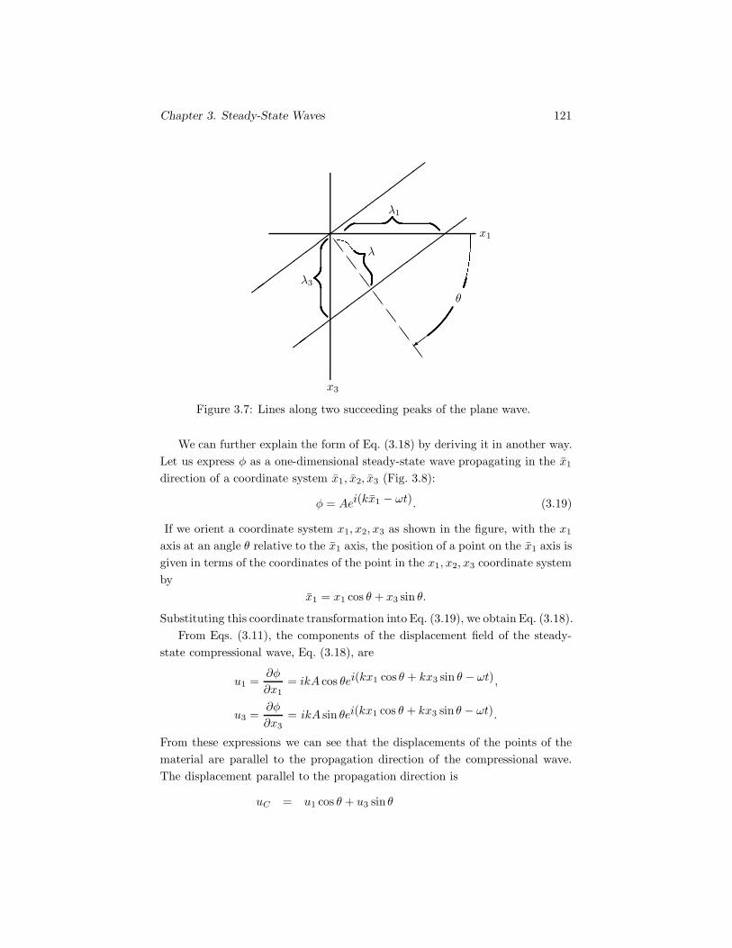
Chapter 3. Steady-State Waves 121
x1
x3
θ
���
��������������
λ1
λ3
λ
��������
��
��
��� �
�������
���
��
��
Figure 3.7: Lines along two succeeding peaks of the plane wave.
We can further explain the form of Eq. (3.18) by deriving it in another way.Let us express φ as a one-dimensional steady-state wave propagating in the x1
direction of a coordinate system x1, x2, x3 (Fig. 3.8):
φ = Aei(kx1 − ωt). (3.19)
If we orient a coordinate system x1, x2, x3 as shown in the figure, with the x1
axis at an angle θ relative to the x1 axis, the position of a point on the x1 axis isgiven in terms of the coordinates of the point in the x1, x2, x3 coordinate systemby
x1 = x1 cos θ + x3 sin θ.
Substituting this coordinate transformation into Eq. (3.19), we obtain Eq. (3.18).From Eqs. (3.11), the components of the displacement field of the steady-
state compressional wave, Eq. (3.18), are
u1 =∂φ
∂x1= ikA cos θei(kx1 cos θ + kx3 sin θ − ωt),
u3 =∂φ
∂x3= ikA sin θei(kx1 cos θ + kx3 sin θ − ωt).
From these expressions we can see that the displacements of the points of thematerial are parallel to the propagation direction of the compressional wave.The displacement parallel to the propagation direction is
uC = u1 cos θ + u3 sin θ

Chapter 3. Steady-State Waves 122
x1
x3
x3
x1
θ
Figure 3.8: One-dimensional plane wave propagating in the direction of thex1 axis.
= ikAei(kx1 cos θ + kx3 sin θ − ωt).
The amplitude of the displacement of the compressional wave is |uC | = k|A|.Equation (3.18) is a convenient expression for a plane compressional wave
with propagation direction θ relative to the x1 axis. We can obtain an expressionfor a plane shear wave with propagation direction θ relative to the x1 axis byassuming a solution for the potential ψ of the same form:
ψ = Cei(kSx1 cos θ + kSx3 sin θ − ωt), (3.20)
where the wave number kS = ω/β. From Eqs. (3.11), the components of thedisplacement field of this steady-state shear wave are
u1 = − ∂ψ
∂x3= −ikSC sin θei(kSx1 cos θ + kSx3 sin θ− ωt),
u3 =∂ψ
∂x1= ikSC cos θei(kSx1 cos θ+ kSx3 sin θ − ωt).
From these expressions we can see that the displacements of the points of thematerial are transverse to the propagation direction of the shear wave. Thedisplacement transverse to the propagation direction is
uS = −u1 sin θ + u3 cos θ
= ikSCei(kSx1 cos θ + kSx3 sin θ − ωt).
The amplitude of the displacement of the shear wave is |uS | = kS|C|.

Chapter 3. Steady-State Waves 123
Plane waves propagating in the x1 direction and attenuatingin the x3 direction
If k21 > ω2/α2, it is convenient to write the solution of Eq. (3.15) in the form
f(x3) = Ae−hx3 +Behx3 ,
where A and B are constants and
h =(k21 −
ω2
α2
)1/2
.
Substituting this form of the solution for f(x3) into Eq. (3.14), we obtain thesolution for the potential φ in the form
φ = Ae−hx3ei(k1x1 − ωt) + Behx3ei(k1x1 − ωt). (3.21)
These solutions represent waves that propagate in the x1 direction and whoseamplitudes attenuate or grow exponentially in the x3 direction. If this expressionis to represent a solution for φ in the half space shown in Fig. 3.5, the constant Bmust be zero since the second term grows without bound in the positive x3
direction. The first term
φ = Ae−hx3ei(k1x1 − ωt) (3.22)
represents a steady-state wave propagating in the x1 direction whose amplitudedecays exponentially in the positive x3 direction. The real part of this solutionis plotted as a function of x1 and x3 in Fig. 3.9.
Equation (3.22) describes a compressional wave. We can obtain an expres-sion for a shear wave that propagates in the x1 direction and whose amplitudedecays exponentially in the positive x3 direction by assuming a solution for thepotential ψ of the same form:
ψ = Ce−hSx3ei(k1x1 − ωt), (3.23)
where
hS =(k21 −
ω2
β2
)1/2
.

Chapter 3. Steady-State Waves 124
x1
x3
Re(φ)
Figure 3.9: A wave propagating in the x1 direction whose amplitude decaysexponentially in the positive x3 direction.

Chapter 3. Steady-State Waves 125
Exercise
Exercise 3.5 A compressional wave is described by the potential
φ = Aei(kx1 cos θ + kx3 sin θ − ωt).
(a) The Lame constants of the material are λ and μ. Determine the stresscomponent T33 as a function of position and time.(b) The density of the material in the reference state is ρ0. Determine thedensity ρ of the material as a function of position and time.
Answer: (a) T33 = −k2φ(λ+ 2μ sin2 θ), (b) ρ = ρ0(1 + k2φ).

Chapter 3. Steady-State Waves 126
3.3 Reflection at a Plane Boundary
Here we determine the solutions for the reflected waves that result when asteady-state plane compressional or shear wave is incident on the free boundaryof a half space of elastic material.
Incident compressional wave
Consider the elastic half space shown in Fig. 3.10, and let us assume that aplane compressional wave with known frequency and known complex amplitudepropagates toward the free boundary of the half space in the direction shown.We can express the compressional wave with a potential of the form of Eq. (3.18):
x1
x3
θ
�������
))))))))
))))))))
Figure 3.10: Elastic half space with a plane compressional wave incident on theboundary.
φ = Iei(kx1 cos θ − kx3 sin θ − ωt), (3.24)
where I is the complex amplitude and the wave number k = ω/α. We havechosen the signs in the exponential term so that the wave propagates in thepositive x1 direction and the negative x3 direction. Our objective is to determinethe wave reflected from the boundary.
The boundary condition at the free boundary of the half space is that thetraction is zero (see Section 1.4):
[tk]x3=0 = [Tmknm]x3=0 = 0.
The unit vector normal to the boundary has components n1 = 0, n2 = 0,n3 = −1, so from this condition we obtain the three stress boundary conditions
[T13]x3=0 = 0, [T23]x3=0 = 0, [T33]x3=0 = 0.
That is, the normal stress and the two components of shear stress on the bound-ary are zero. For the two-dimensional motion we are considering, the stress

Chapter 3. Steady-State Waves 127
component T23 is identically zero. The other two boundary conditions give ustwo conditions that the displacement field must satisfy:
[T13]x3=0 =[μ
(∂u1
∂x3+∂u3
∂x1
)]x3=0
= 0,
[T33]x3=0 =[λ∂u1
∂x1+ (λ+ 2μ)
∂u3
∂x3
]x3=0
= 0.(3.25)
It is easy to show that the boundary conditions cannot be satisfied if weassume that the incident compressional wave causes only a reflected compres-sional wave. The boundary conditions can be satisfied only if we assume thatthere is also a reflected shear wave. Therefore we assume that the compressionalpotential φ and the shear potential ψ are of the forms
φ = Iei(kx1 cos θ − kx3 sin θ − ωt)
+Pei(kx1 cos θP + kx3 sin θP − ωt),
ψ = Sei(kSx1 cos θS + kSx3 sin θS − ωt),
(3.26)
where P and S are the complex amplitudes of the reflected compressional andshear waves. The propagation direction of the reflected compressional waveis θP and the propagation direction of the reflected shear wave is θS (Fig. 3.11).The wave numbers k = ω/α and kS = ω/β. We have chosen the signs so thatthe reflected waves propagate in the positive x1 direction and the positive x3
direction.
x1
x3
θ θP θS
I
P
S
������� �
�������
���������!
)) )) )) ))
********��������
Figure 3.11: The reflected compressional and shear waves.
Chapter 3. Steady-State Waves 128
Substituting Eqs. (3.26) into Eqs. (3.11), we obtain the displacement field
u1 = (u1)I + (u1)P + (u1)S
= ik cos θIei(kx1 cos θ − kx3 sin θ − ωt)
+ik cos θPPei(kx1 cos θP + kx3 sin θP − ωt)
−ikS sin θSSei(kSx1 cos θS + kSx3 sin θS − ωt),
u3 = (u3)I + (u3)P + (u3)S
= −ik sin θIei(kx1 cos θ − kx3 sin θ − ωt)
+ik sin θPPei(kx1 cos θP + kx3 sin θP − ωt)
+ikS cos θSSei(kSx1 cos θS + kSx3 sin θS − ωt),
(3.27)
where the subscripts I, P , and S refer to the incident, compressional, and shearwaves. Substituting these expressions into the boundary conditions, we obtainthe two equations
−[λ cos2 θ+ (λ+ 2μ) sin2 θ]k2Iei(kx1 cos θ − ωt)
−[λ cos2 θP + (λ + 2μ) sin2 θP ]k2Pei(kx1 cos θP − ωt)
−2μk2S sin θS cos θSSe
i(kSx1 cos θS − ωt) = 0,
2k2 sin θ cos θIei(kx1 cos θ − ωt)
−2k2 sin θP cos θPPei(kx1 cos θP − ωt)
+k2S(sin2 θS − cos2 θS)Sei(kSx1 cos θS − ωt) = 0.
(3.28)
The exponential terms in these equations are linearly independent functionsof x1, and therefore the equations have only trivial solutions for the complexamplitudes P and S unless the coefficients of x1 are equal:
k cos θ = k cos θP = kS cos θS . (3.29)
From these relations we see that the propagation direction of the reflected com-pressional wave θP = θ. We also obtain an equation for the propagation direc-tion of the reflected shear wave:
cos θS =k
kScos θ
=β
αcos θ.
(3.30)
Equation (3.29) has an important interpretation. Let λ = 2π/k be thewavelength of the incident and reflected compressional waves and let λS =2π/kS be the wavelength of the reflected shear wave. We can write Eq. (3.29)as
λ
cos θ=
λS
cos θS. (3.31)

Chapter 3. Steady-State Waves 129
Figure 3.12 shows straight lines representing successive crests of the incidentcompressional wave and the reflected shear wave. From this figure we see thatEq. (3.31) implies that the wavelengths of the waves along the boundary areequal:
λB =λ
cos θ=
λS
cos θS.
θ
θS
IS
λB
λ
λS
���� ���
����
������������
������������
Figure 3.12: Successive crests of the incident compressional wave and the re-flected shear wave.
The Poisson’s ratio ν of an elastic material is related to its Lame constantsby (see Exercise 1.29)
ν =λ
2(λ + μ)
From this relation it is easy to show that
β2
α2=
μ
λ + 2μ=
1 − 2ν2(1 − ν)
. (3.32)
With this result, we can express Eq. (3.30), which relates the propagation di-rection θS of the shear wave to the angle θ, in terms of the Poisson’s ratio.Figure 3.13 shows a plot of θS as a function of θ for ν = 0.3.
Because of Eqs. (3.29), the exponential terms cancel from Eqs. (3.28) andwe can write them in the forms
(P/I) +[
2 sin θS cos θS
1 − (2β2/α2) cos2 θ
](S/I) = −1,
(P/I) −[
1 − 2 cos2 θS
(2β2/α2) sin θ cos θ
](S/I) = 1.

Chapter 3. Steady-State Waves 130
0 10 20 30 40 50 60 70 80 900
10
20
30
40
50
60
70
80
90
θ, deg.
θS,deg.
Figure 3.13: The propagation direction of the reflected shear wave for Poisson’sratio ν = 0.3.
We can solve these two equations for the ratios P/I and S/I. Due to Eqs. (3.30)and (3.32), the coefficients of these equations depend only on θ and the Poisson’sratio ν .
From Eq. (3.27), the amplitudes of the displacement of the incident, reflectedcompressional, and reflected shear waves are
|uI| = |(u1)I cos θ − (u3)I sin θ| = k|I|,|uP | = |(u1)P cos θ + (u3)P sin θ| = k|P |,|uS | = |(u1)S sin θS − (u3)S cos θS | = kS |S|.
Figure 3.14 shows plots of the amplitude ratios |uP/uI| = |P/I| and |uS/uI| =|kSS/(kI)| as functions of θ for ν = 0.3. The reflected shear wave vanishes atθ = 0 and at θ = 90◦. The amplitude of the shear wave is a maximum at ap-proximately θ = 40◦, where its amplitude is actually larger than the amplitudeof the incident compressional wave.

Chapter 3. Steady-State Waves 131
0 20 40 60 800
0.2
0.4
0.6
0.8
1
θ, deg.
Amplituderatio
P wave
S wave
Figure 3.14: Amplitude ratios of the reflected compressional and shear wavesfor Poisson’s ratio ν = 0.3.

Chapter 3. Steady-State Waves 132
Incident shear wave
We now assume that a plane shear wave with known frequency and knowncomplex amplitude is incident on the free boundary of an elastic half space.We begin by assuming that it causes a reflected shear wave with propagationdirection θS and a reflected compressional wave with propagation direction θP ,as shown in Fig. 3.15. (We show subsequently that this is true only for aparticular range of values of the propagation direction θ of the incident wave.)
x1
x3
θθP θS
I
P
S
"""""""#��������
���������!
''''''''
********��������
Figure 3.15: Elastic half space with a plane shear wave incident on the boundary.
We write the compressional potential φ and the shear potential ψ in theforms
φ = Pei(kPx1 cos θP + kPx3 sin θP − ωt),
ψ = Iei(kx1 cos θ − kx3 sin θ − ωt)
+Sei(kx1 cos θS + kx3 sin θS − ωt),
(3.33)
where I, P , and S are the complex amplitudes of the incident wave, the reflectedcompressional wave and the reflected shear wave. The wave numbers k = ω/β
and kP = ω/α. From these potentials we obtain the displacement field
u1 = (u1)P + (u1)I + (u1)S
= ikP cos θPPei(kPx1 cos θP + kPx3 sin θP − ωt)
+ik sin θIei(kx1 cos θ − kx3 sin θ − ωt)
−ik sin θSSei(kx1 cos θS + kx3 sin θS − ωt),
u3 = (u3)P + (u3)I + (u3)S
= ikP sin θPPei(kPx1 cos θP + kPx3 sin θP − ωt)
+ik cos θIei(kx1 cos θ − kx3 sin θ − ωt)
+ik cos θSSei(kx1 cos θS + kx3 sin θS − ωt),
(3.34)

Chapter 3. Steady-State Waves 133
where the subscripts I, P , and S refer to the incident, compressional, and shearwaves. Substituting these expressions into the boundary conditions, we obtain
−[λ cos2 θP + (λ + 2μ) sin2 θP ]k2PPe
i(kPx1 cos θP − ωt)
+2μk2 sin θ cos θIei(kx1 cos θ − ωt)
−2μk2 sin θS cos θSSei(kx1 cos θS − ωt) = 0,
−2k2P sin θP cos θPPe
i(kPx1 cos θP − ωt)
+k2(sin2 θ − cos2 θ)Iei(kx1 cos θ − ωt)
+k2(sin2 θS − cos2 θS)Sei(kx1 cos θS − ωt) = 0.
(3.35)
These equations have only trivial solutions for the complex amplitudes P and Sunless the coefficients of x1 are equal:
k cos θ = k cos θS = kP cos θP . (3.36)
Thus θS = θ. The angle between the direction of propagation of the reflectedshear wave and the boundary is equal to the angle between the direction ofpropagation of the incident shear wave and the boundary. The equation for theangle between the direction of propagation of the reflected compressional waveand the boundary is
cos θP =k
kPcos θ
=α
βcos θ.
(3.37)
Let λ = 2π/k be the wavelength of the incident and reflected shear waves andlet λP = 2π/kP be the wavelength of the reflected shear wave. Equation (3.36)states that
λ
cos θ=
λP
cos θP. (3.38)
Figure 3.16 shows straight lines representing successive crests of the incidentshear wave and the reflected compressional wave. The wavelengths of the wavesalong the boundary are equal:
λB =λ
cos θ=
λP
cos θP.
So far, our analysis of the reflection of a shear wave has been similar tothe reflection of a compressional wave. However, at this stage a new and in-teresting phenomenon arises. Recall that the wave speed α of a compressionalwave is larger than the wave speed β of a shear wave. For angles θ such that
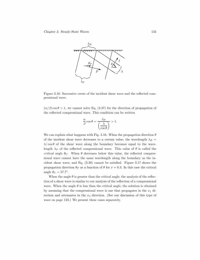
Chapter 3. Steady-State Waves 134
θθPI
P
λB
λP
λ
++++++,����
-----------
--------
----
.......
........
.........
Figure 3.16: Successive crests of the incident shear wave and the reflected com-pressional wave.
(α/β) cos θ > 1, we cannot solve Eq. (3.37) for the direction of propagation ofthe reflected compressional wave. This condition can be written
α
βcos θ =
λP(λ
cos θ
) > 1.
We can explain what happens with Fig. 3.16. When the propagation direction θof the incident shear wave decreases to a certain value, the wavelength λB =λ/ cos θ of the shear wave along the boundary becomes equal to the wave-length λP of the reflected compressional wave. This value of θ is called thecritical angle θC . When θ decreases below this value, the reflected compres-sional wave cannot have the same wavelength along the boundary as the in-cident shear wave, and Eq. (3.38) cannot be satisfied. Figure 3.17 shows thepropagation direction θP as a function of θ for ν = 0.3. In this case the criticalangle θC = 57.7◦.
When the angle θ is greater than the critical angle, the analysis of the reflec-tion of a shear wave is similar to our analysis of the reflection of a compressionalwave. When the angle θ is less than the critical angle, the solution is obtainedby assuming that the compressional wave is one that propagates in the x1 di-rection and attenuates in the x3 direction. (See our discussion of this type ofwave on page 123.) We present these cases separately.

Chapter 3. Steady-State Waves 135
40 50 60 70 80 900
10
20
30
40
50
60
70
80
90
θ, deg.
θP,deg.
Figure 3.17: Propagation direction of the reflected compressional wave for Pois-son’s ratio ν = 0.3.
Angle θ greater than the critical angle θC
Because of Eqs. (3.36), we can write Eqs. (3.35) in the forms
(S/I) −[2(β2/α2) sin θP cos θP
sin2 θ − cos2 θ
](P/I) = −1,
(S/I) +[1 − 2(β2/α2) cos2 θP
2 sin θ cos θ
](P/I) = 1.
(3.39)
We can solve these two equations for the ratios S/I and P/I. As a result ofEqs. (3.32) and (3.37), the coefficients of these equations depend only on θ andthe Poisson’s ratio ν .
From Eq. (3.34), the amplitudes of the displacement of the incident, reflectedshear, and reflected compressional waves are
|uI | = |(u1)I sin θ + (u3)I cos θ| = k|I|,|uS| = |(u1)S sin θ − (u3)S cos θ| = k|S|,|uP | = |(u1)P cos θP + (u3)P sin θP | = kP |P |.

Chapter 3. Steady-State Waves 136
With these relations and the solutions of Eqs. (3.39), we can determine theamplitude ratios |uS/uI| = |S/I| and |uP/uI | = |kPP/(kI)| as functions of θfor angles greater than the critical angle.
Angle θ less than the critical angle θC
In this case the boundary conditions cannot be satisfied by assuming that thereis a reflected compressional wave. Instead, we assume that the compressionalwave propagates in the x1 direction and attenuates in the x3 direction. To doso, we write the compressional potential φ in the form of Eq. (3.22):
φ = Pe−hx3ei(kPx1 − ωt),
ψ = Iei(kx1 cos θ − kx3 sin θ − ωt)
+Sei(kx1 cos θS + kx3 sin θS − ωt),
(3.40)
where
h =(k2
P − ω2
α2
)1/2
.
The wave number k = ω/β. From these potentials we obtain the displacementfield
u1 = (u1)P + (u1)I + (u1)S
= ikPPe−hx3ei(kPx1 − ωt)
+ik sin θIei(kx1 cos θ − kx3 sin θ − ωt)
−ik sin θSSei(kx1 cos θS + kx3 sin θS − ωt),
u3 = (u3)P + (u3)I + (u3)S
= −hPe−hx3ei(kPx1 − ωt)
+ik cos θIei(kx1 cos θ − kx3 sin θ− ωt)
+ik cos θSSei(kx1 cos θS + kx3 sin θS − ωt).
(3.41)
where the subscripts I, P , and S refer to the incident, compressional, and shearwaves. Substituting these expressions into the boundary conditions, Eqs. (3.25),we obtain
[−λk2P + (λ + 2μ)h2]Pei(kPx1 − ωt)
+2μk2 sin θ cos θIei(kx1 cos θ − ωt)
−2μk2 sin θS cos θSSei(kx1 cos θS − ωt) = 0,
−2ikPhPei(kPx1 − ωt)
+k2(sin2 θ − cos2 θ)Iei(kx1 cos θ − ωt)
+k2(sin2 θS − cos2 θS)Sei(kx1 cos θS − ωt) = 0.
(3.42)

Chapter 3. Steady-State Waves 137
These equations have only trivial solutions for the complex amplitudes P and Sunless
k cos θ = kP . (3.43)
By using this result, we can write Eqs. (3.42) in the forms
(S/I) −[2i cos θ(cos2 θ − β2/α2)1/2
sin2 θ − cos2 θ
](P/I) = −1,
(S/I) +[1 − 2 cos2 θ2 sin θ cos θ
](P/I) = 1.
(3.44)
From Eqs. (3.41), the amplitudes of the displacement of the incident andreflected shear waves are
|uI| = |(u1)I sin θ + (u3)I cos θ| = k|I|,|uS| = |(u1)S sin θ − (u3)S cos θ| = k|S|,
and the amplitude of the horizontal motion of the compressional wave at x3 = 0is
|(u1)P | = kP |P | = k cos θ|P |.
With these relations and the solutions of Eqs. (3.44), we can determine theamplitude ratios |uS/uI| = |S/I| and |(u1)P/uI | = cos θ|P/I| as functions of θfor angles less than the critical angle.
Figure 3.18 shows the amplitude ratios of the shear and compressional wavesas functions of θ for ν = 0.3. (For angles below the critical angle θC , we plot theamplitude ratio of the horizontal motion of the compressional wave at x3 = 0.)Below the critical angle, the amplitude of the reflected shear wave is equal tothe amplitude of the incident shear wave.

Chapter 3. Steady-State Waves 138
0 10 20 30 40 50 60 70 80 900
0.2
0.4
0.6
0.8
1
1.2
1.4
1.6
1.8
2
θCθ, deg.
Amplituderatio
P waveS wave
Figure 3.18: Amplitude ratios of the reflected shear and compressional wavesfor Poisson’s ratio ν = 0.3.

Chapter 3. Steady-State Waves 139
Exercise
Exercise 3.6 The motion of an elastic material is described by the displace-ment field
u1 = 0,u2 = u2(x1, x3, t),u3 = 0.
(a) Show that u2 satisfies the wave equation
∂2u2
∂t2= β2
(∂2u2
∂x21
+∂2u2
∂x23
).
x1
x3
θ θR
�������
������� (
(((((/
))))))))
))))))))
For the half-space shown, suppose that the displacement field consists of theincident and reflected waves
u2 = Iei(kx1 cos θ − kx3 sin θ − ωt)
+ Rei(kx1 cos θR + kx3 sin θR − ωt).
(b) Show that k = ω/β.(c) Show that θR = θ and R = I.
Discussion—The waves described in this exercise are horizontally polarizedshear waves. They are plane waves that propagate in the x1-x3 plane, but themotion of the material particles is perpendicular to the x1-x3 plane.
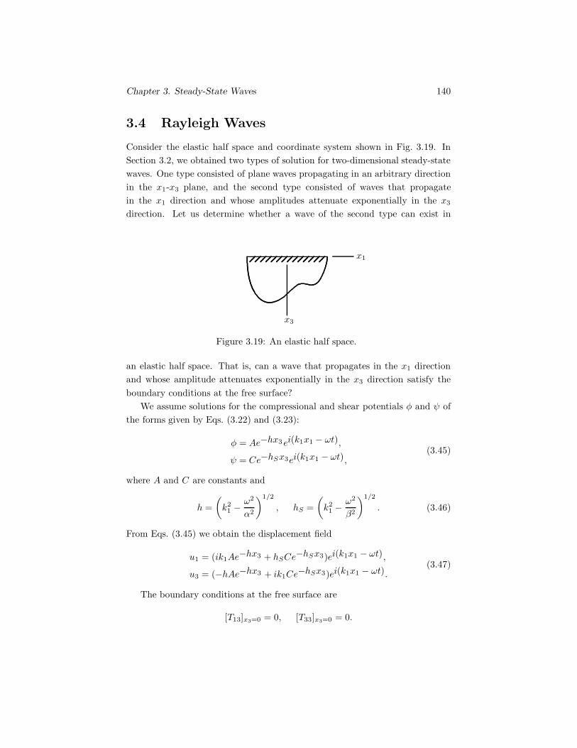
Chapter 3. Steady-State Waves 140
3.4 Rayleigh Waves
Consider the elastic half space and coordinate system shown in Fig. 3.19. InSection 3.2, we obtained two types of solution for two-dimensional steady-statewaves. One type consisted of plane waves propagating in an arbitrary directionin the x1-x3 plane, and the second type consisted of waves that propagatein the x1 direction and whose amplitudes attenuate exponentially in the x3
direction. Let us determine whether a wave of the second type can exist in
x1
x3
Figure 3.19: An elastic half space.
an elastic half space. That is, can a wave that propagates in the x1 directionand whose amplitude attenuates exponentially in the x3 direction satisfy theboundary conditions at the free surface?
We assume solutions for the compressional and shear potentials φ and ψ ofthe forms given by Eqs. (3.22) and (3.23):
φ = Ae−hx3ei(k1x1 − ωt),
ψ = Ce−hSx3ei(k1x1 − ωt),(3.45)
where A and C are constants and
h =(k21 − ω2
α2
)1/2
, hS =(k21 −
ω2
β2
)1/2
. (3.46)
From Eqs. (3.45) we obtain the displacement field
u1 = (ik1Ae−hx3 + hSCe
−hSx3)ei(k1x1 − ωt),
u3 = (−hAe−hx3 + ik1Ce−hSx3)ei(k1x1 − ωt).
(3.47)
The boundary conditions at the free surface are
[T13]x3=0 = 0, [T33]x3=0 = 0.

Chapter 3. Steady-State Waves 141
From Eq. (3.25), the expressions for the boundary conditions in terms of dis-placements are[
μ
(∂u1
∂x3+∂u3
∂x1
)]x3=0
= 0,[λ∂u1
∂x1+ (λ + 2μ)
∂u3
∂x3
]x3=0
= 0.
Substituting Eqs. (3.47) into these boundary conditions, we obtain a system ofhomogeneous equations for the constants A and C that we write as[
2ik1h 2k21 − ω2/β2
2k21 − ω2/β2 −2ik1hS
] [AC
]= 0. (3.48)
This system has a nontrivial solution for A and C only if the determinant ofthe coefficients is equal to zero:
4k21hhS −
(2k2
1 − ω2
β2
)2
= 0. (3.49)
We denote the phase velocity of the wave in the x1 direction by
cR =ω
k1.
By using Eqs. (3.46), we can write Eq. (3.49) in terms of cR in the form
(2 − c2R
β2
)2
− 4(
1 − β2
α2
c2Rβ2
)1/2 (1 − c2R
β2
)1/2
= 0. (3.50)
This expression is called the Rayleigh characteristic equation. It has one rootwhich yields a wave that propagates in the x1 direction and whose amplitudeattenuates exponentially in the x3 direction. This type of wave is called a surfacewave, because it has significant amplitude only near the surface. The particularexample we have derived is called a Rayleigh wave.
From Eq. (3.32), we see that the solution of Eq. (3.50) for cR/β dependsonly on the value of the Poisson’s ratio ν of the material. Figure 3.20 shows aplot of the value of cR/β as a function of Poisson’s ratio. The Rayleigh wavephase velocity is slightly less than the shear wave velocity.
From Eq. (3.48), we can write the constant C in terms of the constant A as
C =2ik1h
ω2
β2− 2k2
1
A.
Substituting this result into Eqs. (3.47), we obtain expressions for the displace-ment components in terms of A. The real parts of the resulting equations can
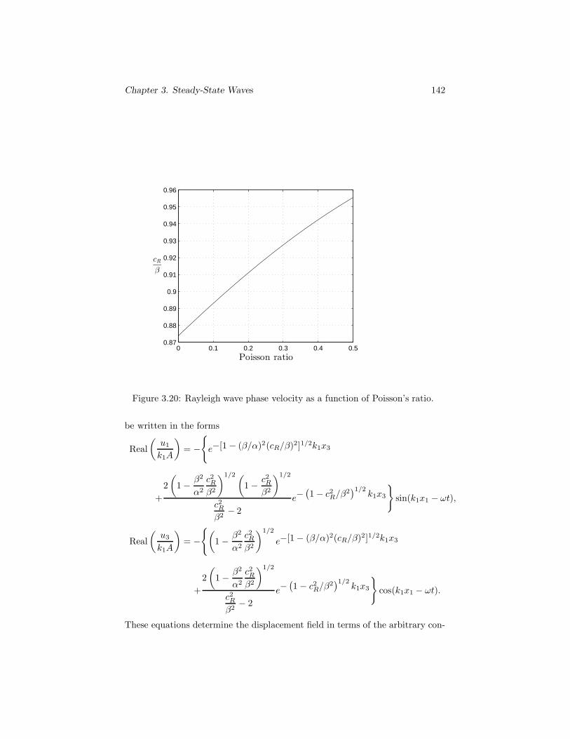
Chapter 3. Steady-State Waves 142
0 0.1 0.2 0.3 0.4 0.50.87
0.88
0.89
0.9
0.91
0.92
0.93
0.94
0.95
0.96
Poisson ratio
cRβ
Figure 3.20: Rayleigh wave phase velocity as a function of Poisson’s ratio.
be written in the forms
Real(u1
k1A
)= −
{e−[1 − (β/α)2(cR/β)2]1/2k1x3
+2(
1 − β2
α2
c2Rβ2
)1/2 (1 − c2R
β2
)1/2
c2Rβ2
− 2e−
(1 − c2R/β
2)1/2
k1x3
}sin(k1x1 − ωt),
Real(u3
k1A
)= −
{(1 − β2
α2
c2Rβ2
)1/2
e−[1 − (β/α)2(cR/β)2]1/2k1x3
+2(
1 − β2
α2
c2Rβ2
)1/2
c2Rβ2
− 2e−
(1 − c2R/β
2)1/2
k1x3
}cos(k1x1 − ωt).
These equations determine the displacement field in terms of the arbitrary con-

Chapter 3. Steady-State Waves 143
stant A. The wave number k1 = ω/cR depends on the frequency. For a givenPoisson’s ratio ν , we can hold the position fixed and determine the displacementcomponents of a point as functions of time. Figure 3.21 shows the resulting tra-
k1x1
k1x3
Counterclockwise
Clockwise
Clockwise
Clockwise
0 2 4
0
2
4
6
........
........
..............................................
..........................................................................................................................................................................................................................................................
........
........
........
........
........
.....................................................................................................................................................................
........
........
.......................................................................................................
........
.................................................
.......
Figure 3.21: Particle trajectories at the surface and at several depths for Pois-son’s ratio ν = 0.3.
jectories of points of the material at depths k1x3 = 0, 2, 4, and 6 for a Rayleighwave propagating in the positive x1 direction. The points of the material movein elliptical paths. The points near the surface move in the counterclockwise di-rection. At approximately k1x3 = 1, the horizontal motion vanishes, and belowthat depth the points move in the clockwise direction.
3.5 Steady-State Waves in a Layer
We want to analyze the propagation of waves along a layer of elastic material.So that some of the concepts can be more easily understood, we first discussthe simpler case of acoustic waves in a channel.
Acoustic waves in a channel
The theory of acoustic or sound waves can be obtained from the equationsof linear elastic wave propagation by setting the shear modulus μ = 0. (Seepage 44.) Shear waves do not exist, and the displacement field can be expressed

Chapter 3. Steady-State Waves 144
in terms of the potential φ:u = ∇φ.
Suppose that an acoustic medium occupies the space between two unbounded,rigid plates, as shown in Fig. 3.22, and consider two-dimensional motion of themedium described by the displacement field
u1 = u1(x1, x3, t),u2 = 0,u3 = u3(x1, x3, t).
In terms of φ, the displacement field is
x1
x3
2h
�
�
Figure 3.22: Acoustic medium between two unbounded rigid plates.
u1 =∂φ
∂x1, u3 =
∂φ
∂x3.
We assume a solution for φ that describes a steady-state wave propagating alongthe channel:
φ = f(x3)ei(k1x1 − ωt),
where the function f(x3) that describes the distribution of φ across the chan-nel must be determined. This is the same form of solution we discussed inSection 3.2. Substituting it into the wave equation
∂2φ
∂t2= α2
(∂2φ
∂x21
+∂2φ
∂x23
),
we find that the function f(x3) must satisfy the equation
d2f(x3)dx2
3
+(ω2
α2− k2
1
)f(x3) = 0.
In this case we express the solution of this equation in the form
f(x3) = A sin k3x3 + B cos k3x3,
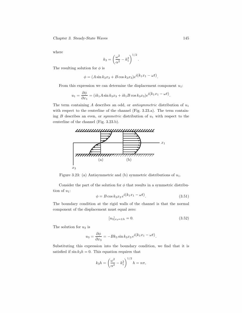
Chapter 3. Steady-State Waves 145
where
k3 =(ω2
α2− k2
1
)1/2
.
The resulting solution for φ is
φ = (A sin k3x3 + B cos k3x3)ei(k1x1 − ωt).
From this expression we can determine the displacement component u1:
u1 =∂φ
∂x1= (ik1A sin k3x3 + ik1B cos k3x3)ei(k1x1 − ωt).
The term containing A describes an odd, or antisymmetric distribution of u1
with respect to the centerline of the channel (Fig. 3.23.a). The term contain-ing B describes an even, or symmetric distribution of u1 with respect to thecenterline of the channel (Fig. 3.23.b).
x1
x3
(a)
�����
�����
(b)
������
�����
Figure 3.23: (a) Antisymmetric and (b) symmetric distributions of u1.
Consider the part of the solution for φ that results in a symmetric distribu-tion of u1:
φ = B cos k3x3 ei(k1x1 − ωt). (3.51)
The boundary condition at the rigid walls of the channel is that the normalcomponent of the displacement must equal zero:
[u3]x3=±h = 0. (3.52)
The solution for u3 is
u3 =∂φ
∂x3= −Bk3 sink3x3 e
i(k1x1 − ωt).
Substituting this expression into the boundary condition, we find that it issatisfied if sin k3h = 0. This equation requires that
k3h =(ω2
α2− k2
1
)1/2
h = nπ,

Chapter 3. Steady-State Waves 146
where n is any integer. We can solve this equation for the wave number k1 as afunction of the frequency:
k1 =(ω2
α2− n2π2
h2
)1/2
. (3.53)
With this result, we can also solve for the phase velocity of the wave in the x1
direction c1 = ω/k1 as a function of the frequency:
c1α
=1[
1 −(αnπωh
)2]1/2
. (3.54)
For a given frequency ω and integer n, we can substitute Eq. (3.53) intoEq. (3.51) to determine the potential φ. Thus we have obtained an infinitenumber of solutions that satisfy the boundary condition. These solutions arecalled propagation modes, or simply modes. The solution for n = 0 is calledthe first mode, the solution for n = 1 is called the second mode, and so forth.
The solutions of Eq. (3.54) for the phase velocities of the modes are shown asfunctions of frequency in Fig. 3.24. The phase velocities of all the modes except
0 0.5 1 1.5 2 2.5 3 3.5 40
0.5
1
1.5
2
2.5
3
3.5
4
ωh
πα
c1α
n = 0
n = 1
n = 2n = 3
c1α
n = 0
n = 1
n = 2n = 3
c1α
n = 0
n = 1
n = 2n = 3
c1α
n = 0
n = 1
n = 2n = 3
Figure 3.24: Phase velocities of the modes as functions of frequency.
the first one depend on the frequency. When the phase velocity of a wave varieswith the frequency, the wave is said to be dispersive, or to exhibit dispersion.

Chapter 3. Steady-State Waves 147
For this reason, Eqs. (3.53) and (3.54) are called dispersion relations. In thisexample all of the modes except the first one are dispersive.
The phase velocities of all of the modes except the first one approach in-finity when the frequency approaches the value ω = αnπ/h. From Eq. (3.53),we see that when the frequency approaches this value the wave number k1 ap-proaches zero (which means that the wavelength of the wave in the x1 directionapproaches infinity), and below this frequency the wave number k1 is imaginary.When k1 is imaginary Eq. (3.51) does not describe a propagating wave, but os-cillates in time and attenuates exponentially in the x1 direction. The frequenciesbelow which the wave number is imaginary are called cutoff frequencies. Amode does not propagate when the frequency is below its cutoff frequency.
Figure 3.25 shows the distributions of u1 as a function of x3 for the firstthree modes. The first mode is one-dimensional motion: the distribution of u1
is uniform and u3 = 0. This mode propagates at the wave speed α for anyfrequency.
x1
x3
n = 0
�����������������
n = 1
���
�
�
�
�
�
�
�
�
�
�
�
�
n = 2
���
�
�
�
�
�
�
�
�
�
�
Figure 3.25: Distributions of u1 for the first three modes.
Waves in an elastic layer
We now turn to the propagation of two-dimensional steady-state waves alonga plate of elastic material with free surfaces (Fig. 3.26). The analysis is verysimilar to our treatment of acoustic waves in a channel in the previous section.
We consider two-dimensional motion described by the displacement field
u1 = u1(x1, x3, t),u2 = 0,u3 = u3(x1, x3, t).
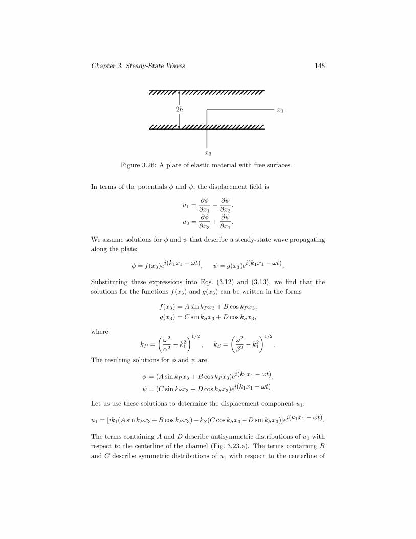
Chapter 3. Steady-State Waves 148
x1
x3
2h
�
�
Figure 3.26: A plate of elastic material with free surfaces.
In terms of the potentials φ and ψ, the displacement field is
u1 =∂φ
∂x1− ∂ψ
∂x3,
u3 =∂φ
∂x3+∂ψ
∂x1.
We assume solutions for φ and ψ that describe a steady-state wave propagatingalong the plate:
φ = f(x3)ei(k1x1 − ωt), ψ = g(x3)ei(k1x1 − ωt).
Substituting these expressions into Eqs. (3.12) and (3.13), we find that thesolutions for the functions f(x3) and g(x3) can be written in the forms
f(x3) = A sin kPx3 + B cos kPx3,
g(x3) = C sin kSx3 +D cos kSx3,
where
kP =(ω2
α2− k2
1
)1/2
, kS =(ω2
β2− k2
1
)1/2
.
The resulting solutions for φ and ψ are
φ = (A sin kPx3 + B cos kPx3)ei(k1x1 − ωt),
ψ = (C sin kSx3 +D cos kSx3)ei(k1x1 − ωt).
Let us use these solutions to determine the displacement component u1:
u1 = [ik1(A sin kPx3 +B cos kPx3)−kS(C cos kSx3−D sin kSx3)]ei(k1x1 − ωt).
The terms containing A and D describe antisymmetric distributions of u1 withrespect to the centerline of the channel (Fig. 3.23.a). The terms containing Band C describe symmetric distributions of u1 with respect to the centerline of
Chapter 3. Steady-State Waves 149
the channel (Fig. 3.23.b). Consider the parts of the solutions for φ and ψ thatresult in a symmetric distribution of u1:
φ = B cos kPx3 ei(k1x1 − ωt), ψ = C sin kSx3 e
i(k1x1 − ωt). (3.55)
The resulting expressions for u1 and u3 are
u1 = (ik1B cos kPx3 − kSC cos kSx3)ei(k1x1 − ωt),
u3 = (−kPB sin kPx3 + ik1C sin kSx3)ei(k1x1 − ωt).(3.56)
The boundary conditions at the free surfaces of the plate are
[T13]x3=±h =[μ
(∂u1
∂x3+∂u3
∂x1
)]x3=±h
= 0,
[T33]x3=±h =[λ∂u1
∂x1+ (λ+ 2μ)
∂u3
∂x3
]x3=±h
= 0.(3.57)
Substituting Eqs. (3.56) into these boundary conditions, we obtain two homo-geneous equations in terms of B and C:[
[2μk21 − (λ+ 2μ)ω2/α2] cos kPh 2iμk1kS cos kSh
−2ik1kP sin kPh (ω2/β2 − 2k21) sin kSh
] [BC
]= 0.
This system has a nontrivial solution for B and C only if the determinant ofthe coefficients is equal to zero:
[2μk21 − (λ + 2μ)ω2/α2](ω2/β2 − 2k2
1) cos kPh sin kSh
−4μk21kPkS sin kPh cos kSh = 0.
This is the dispersion relation for symmetric longitudinal waves in a layer. Itdetermines the wave number k1 as a function of the frequency. If we express itin terms of the phase velocity in the x1 direction c1 = ω/k1, it can be writtenin the form
(2 − c21
β2
)2tan
[(1 − β2
c21
)1/2ωh
β
]
tan
[(β2
α2− β2
c21
)1/2ωh
β
] + 4(c21β2
β2
α2− 1
)1/2 (c21β2
− 1)1/2
= 0.
(3.58)For a given frequency ω, this equation can be solved numerically for the phasevelocity c1. The equation is transcendental, and has an infinite number of roots.Each root yields a propagation mode that satisfies the boundary conditions atthe free surfaces of the plate. These solutions are called the Rayleigh-Lambmodes.

Chapter 3. Steady-State Waves 150
The solution for c1/β as a function of ωh/β depends only on the param-eter β/α. From Eq. (3.32), we see that this parameter depends only on thePoisson’s ratio ν of the material. Figure 3.27 shows a plot c1/β as a functionof ωh/β for the first and second propagation modes for ν = 0.3. This figure is
0 1 2 3 4 5 6 7 80
0.5
1
1.5
2
2.5
3
3.5
4
ωh
β
c1β
cRβ
mode 1
mode 2c1β
cRβ
mode 1
mode 2
Figure 3.27: Phase velocities of the first two Rayleigh-Lamb modes as functionsof frequency.
qualitatively similar to Fig. 3.24 for acoustic waves in a channel. However, inthe acoustic problem the first mode was not dispersive. In the case of wavesalong an elastic plate, even the first mode is dispersive. At high frequency,the phase velocities of the modes approach the Rayleigh-wave phase velocity cR(Section 3.4).
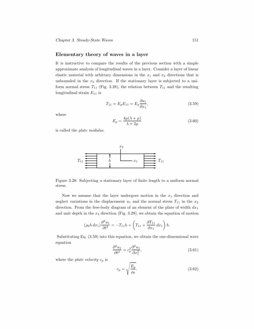
Chapter 3. Steady-State Waves 151
Elementary theory of waves in a layer
It is instructive to compare the results of the previous section with a simpleapproximate analysis of longitudinal waves in a layer. Consider a layer of linearelastic material with arbitrary dimensions in the x1 and x2 directions that isunbounded in the x3 direction. If the stationary layer is subjected to a uni-form normal stress T11 (Fig. 3.28), the relation between T11 and the resultinglongitudinal strain E11 is
T11 = EpE11 = Ep∂u1
∂x1, (3.59)
where
Ep =4μ(λ+ μ)λ+ 2μ
(3.60)
is called the plate modulus.
x1
x2
hT11 T11
�
� �������
�������
Figure 3.28: Subjecting a stationary layer of finite length to a uniform normalstress.
Now we assume that the layer undergoes motion in the x1 direction andneglect variations in the displacement u1 and the normal stress T11 in the x2
direction. From the free-body diagram of an element of the plate of width dx1
and unit depth in the x3 direction (Fig. 3.29), we obtain the equation of motion
(ρ0h dx1)∂2u1
∂t2= −T11h+
(T11 +
∂T11
∂x1dx1
)h.
Substituting Eq. (3.59) into this equation, we obtain the one-dimensional waveequation
∂2u1
∂t2= c2p
∂2u1
∂x21
, (3.61)
where the plate velocity cp is
cp =
√Ep
ρ0. (3.62)
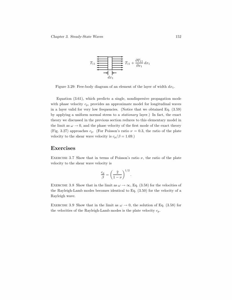
Chapter 3. Steady-State Waves 152
dx1
T11 T11 +∂T11
∂x1dx1
���������
�������
Figure 3.29: Free-body diagram of an element of the layer of width dx1.
Equation (3.61), which predicts a single, nondispersive propagation modewith phase velocity cp, provides an approximate model for longitudinal wavesin a layer valid for very low frequencies. (Notice that we obtained Eq. (3.59)by applying a uniform normal stress to a stationary layer.) In fact, the exacttheory we discussed in the previous section reduces to this elementary model inthe limit as ω → 0, and the phase velocity of the first mode of the exact theory(Fig. 3.27) approaches cp. (For Poisson’s ratio ν = 0.3, the ratio of the platevelocity to the shear wave velocity is cp/β = 1.69.)
Exercises
Exercise 3.7 Show that in terms of Poisson’s ratio ν , the ratio of the platevelocity to the shear wave velocity is
cpβ
=(
21 − ν
)1/2
.
Exercise 3.8 Show that in the limit as ω → ∞, Eq. (3.58) for the velocities ofthe Rayleigh-Lamb modes becomes identical to Eq. (3.50) for the velocity of aRayleigh wave.
Exercise 3.9 Show that in the limit as ω → 0, the solution of Eq. (3.58) forthe velocities of the Rayleigh-Lamb modes is the plate velocity cp.

Chapter 3. Steady-State Waves 153
Exercise 3.10
x1
x3
upper material
lower material
$$$$
%%%%
A wave analogous to a Rayleigh wave can exist at a plane, bonded interfacebetween two different elastic materials. This wave, called a Stoneley wave,attenuates exponentially with distance away from the interface in each material.Derive the characteristic equation for a Stoneley wave.

Chapter 3. Steady-State Waves 154
3.6 Steady-State Waves in Layered Media
Layered media occur in nature, and are also manufactured by bonding layers ofdifferent materials together to obtain composite materials with desired mechan-ical properties. A wave propagating through a layered elastic medium behavesquite differently from a wave in a homogeneous medium, due to the effects of theinterfaces between the layers. In this section, we consider steady-state waves ina medium consisting of alternating plane layers of two elastic materials a and b(Fig. 3.30). Two adjacent layers form what is called a unit cell of the material.
x1
d
da db
��
�� ��
unit cell
$$$$$$$$
$$$$$$$$
$$
$$$$
$$$$$$$$$$
$$$$$$$$$$$$$$
Figure 3.30: Medium of alternating layers of elastic materials a and b.
Suppose that a plane compressional steady-state wave propagates in the x1
direction perpendicular to the interfaces between layers. Let the subscript ξdenote either a or b. The displacement within each layer of a unit cell is governedby the one-dimensional wave equation:
∂2uξ
∂t2= α2
ξ
∂2uξ
∂x21
.
We express the solution within each layer as a sum of forward and rearwardpropagating waves,
uξ = Aξei(kξx1 − ωt) +Bξe
i(−kξx1 − ωt), (3.63)
where the wave number kξ iskξ =
ω
αξ. (3.64)
In terms of the displacement, the normal stress T11 within each layer is
Tξ = ρξα2ξ
∂uξ
∂x1=z2ξ
ρξ
∂uξ
∂x1, (3.65)

Chapter 3. Steady-State Waves 155
where the acoustic impedance zξ = ρξαξ.Let x1 = 0 be the interface between the layers of the unit cell (Fig. 3.31).
The displacements and normal stresses in the two materials must be equal at
material a material b
x1
x1 = −da x1 = 0 x1 = db
%%%%$$$$
$$$$$
$$
$$
$$
$$$
$$
$$
$$
$$
$$
$$$
$$
$$
$$
$$$$$$$$$
$$$$$$
$$$$$
$$$
$$
Figure 3.31: A unit cell.
the interface:
ua(0, t) = ub(0, t), (3.66)
Ta(0, t) = Tb(0, t). (3.67)
Because the solutions given by Eq. (3.63) contain four constants, Aa, Ba, Ab,and Bb, two more conditions are needed. We obtain them from the periodicityof the problem with a result called the Floquet theorem. We recast Eqs. (3.63)and (3.65) into steady-state wave expressions having the same wave number kfor both materials,
uξ = Uξ(x1)ei(kx1 − ωt), (3.68)
Tξ = Tξ(x1)ei(kx1 − ωt), (3.69)
where we define
Uξ(x1) = AξeiK−
ξ x1 + Bξe−iK+
ξ x1 ,
Tξ(x1) = izξω[AξeiK−
ξ x1 − Bξe−iK+
ξ x1 ],
andK±
ξ = kξ ± k.

Chapter 3. Steady-State Waves 156
Because the functions Uξ(x1) and Tξ(x1) are continuous across the layer inter-faces and do not depend on time, the Floquet theorem states that they must beperiodic functions of x1 with period equal to the length d = da + db of the unitcell:
Ua(−da) = Ub(db), (3.70)
Ta(−da) = Tb(db). (3.71)
We can write these two conditions, together with Eqs. (3.66) and (3.67), inmatrix form as⎡⎢⎢⎢⎢⎣
1 1 1 1za −za zb −zb
e−iK−a da eiK
+a da eiK
−b db e−iK
+b db
zae−iK−
a da −zaeiK+
a da zbeiK−
b db −zbe−iK+
b db
⎤⎥⎥⎥⎥⎦⎡⎢⎢⎣
Aa
Ba
−Ab
−Bb
⎤⎥⎥⎦ = [0].
(3.72)Equating the determinant of the coefficients to zero, we obtain
cos kd = cos(ωda
αa
)cos
(ωdb
αb
)− 1
2
(za
zb+zb
za
)sin
(ωda
αa
)sin
(ωdb
αb
).
(3.73)
This is the dispersion relation for the steady-state wave. For a given frequency ω,we can solve it for the wave number k and then determine the phase velocityc1 = ω/k.
Special cases
When za = zb, Eq. (3.73) yields a simple expression for the phase velocity c1 interms of the compressional wave speeds of the two materials:
d
c1=da
αa+db
αb. (3.74)
If, in addition, αa = αb = α, the two materials are identical and c1 = α.In the limit ω → 0, the solution for the phase velocity is
c1 =d
Δd, (3.75)
where
Δ2d =
(da
αa
)2
+(za
zb+zb
za
)dadb
αaαb+
(db
αb
)2
. (3.76)
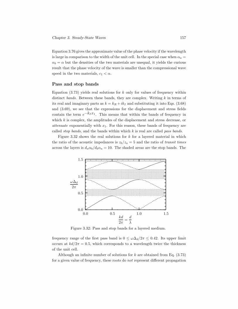
Chapter 3. Steady-State Waves 157
Equation 3.76 gives the approximate value of the phase velocity if the wavelengthis large in comparison to the width of the unit cell. In the special case when αa =αb = α but the densities of the two materials are unequal, it yields the curiousresult that the phase velocity of the wave is smaller than the compressional wavespeed in the two materials, c1 < α.
Pass and stop bands
Equation (3.73) yields real solutions for k only for values of frequency withindistinct bands. Between these bands, they are complex. Writing k in terms ofits real and imaginary parts as k = kR + ikI and substituting it into Eqs. (3.68)and (3.69), we see that the expressions for the displacement and stress fieldscontain the term e−kIx1 . This means that within the bands of frequency inwhich k is complex, the amplitudes of the displacement and stress decrease, orattenuate exponentially with x1. For this reason, these bands of frequency arecalled stop bands, and the bands within which k is real are called pass bands.
Figure 3.32 shows the real solutions for k for a layered material in whichthe ratio of the acoustic impedances is zb/za = 5 and the ratio of transit timesacross the layers is daαb/dbαa = 10. The shaded areas are the stop bands. The
kd
2π=d
λ
ωΔd
2π
0.0 0.5 1.0 1.50.0
0.5
1.0
1.5
...
...................................................................................................................................................................................................................................................................................................................................................................................................................................................
...
...
...
...
...
...
...
...
...
...
...
...
...
...
...
...
...
...
...
...
...
...
...
...
...
...
...
...
...
...
...
...
...
...
...
...
...
...
...
...
...
...
...
...
...
...
...
...
...
...
...
...
...
...
...
...
...
...
...
...
...
...
...
...
...
...
...
...
...
...
...
...
...
...
...
...
...
...
...
...
...
...
...
...
...
...
...
...
...
...
...
...
...
...
...
...
...
...
...
...
...
...
...
...
...
...
...
...
...
...
...
...
...
...
...
...
...
...
...
...
...
...
...
...
...
...
...
...
...
...
...
...
...
...
...
...
...
...
...
...
...
...
...
...
...
...
...
...
...
...
...
...
...
...
...
...
...
...
...
...
...
...
...
...
...
...
...
...
...
...
...
...
...
...
...
...
...
...
...
...
...
...
...
...
...
...
...
...
...
...
...
...
...
...
...
...
...
...
...
...
...
...
...
...
...
...
...
...
...
...
...
...
...
...
...
...
...
...
...
...........................................................................................................................................................................................................................
...............................
..............................
.............................
...............................
....................................
........................................
...........................................................................................................................................................................................
.....................................................
..............................................
...............................................
....................................
.......................
..................
..................
...................
........................
..................
.......................
..................
..................
...................
........................
..................
..................................................................................................................
..................................................................................................................
.................................
............................
.............................
....................
.................................
............................
.............................
....................
Figure 3.32: Pass and stop bands for a layered medium.
frequency range of the first pass band is 0 ≤ ωΔd/2π ≤ 0.42. Its upper limitoccurs at kd/2π = 0.5, which corresponds to a wavelength twice the thicknessof the unit cell.
Although an infinite number of solutions for k are obtained from Eq. (3.73)for a given value of frequency, these roots do not represent different propagation
Chapter 3. Steady-State Waves 158
modes. They result in identical solutions for the displacement field, so there is asingle propagation mode. To emphasize this point, we plot only one “branch” ofeach pass band as a solid line and show the other branches as dashed lines. Asthe ratio of the acoustic impedances of the two materials approaches one, thestop bands narrow, and the branches we show as solid lines approach a singlestraight line, the dispersion relation of the resulting homogeneous material.
When superimposed waves having different frequencies propagate through alayered medium, the waves having frequencies within stop bands are attenuated,altering the character of the superimposed wave. We examine this phenomenonin the next chapter.
Exercises
Exercise 3.11 Show that when za = zb, Eq. (3.73) yields the expression givenin Eq. (3.74) for the phase velocity c1 = ω/k in a layered material.
Exercise 3.12 Show that in the limit ω → 0, the solution of Eq. (3.73) for thephase velocity of a steady-state wave in a layered material is given by Eq. (3.75).
Exercise 3.13 For the layered material discussed in Section 3.6, the fractionof the volume of the material occupied by material a is φ = da/(da +db) = da/d.Derive an equation for the low-frequency limit of the phase velocity as a functionof φ. Using the properties of tungsten for material a and aluminum for material b(see Table B.2 in Appendix B), plot your equation for values of φ from zero toone.
Chapter 4
Transient Waves
Analytical and numerical solutions to transient wave problemsin elastic materials can be obtained by integral transform methods,particularly Fourier and Laplace transforms. We discuss these trans-forms in the next two sections. We then define the discrete Fouriertransform and demonstrate the use of the numerical algorithm calledthe fast Fourier transform (FFT). In the concluding section, we in-troduce the most important technique for transient waves in elasticwave propagation, the Cagniard-de Hoop method, by determiningthe response of an elastic half space to an impulsive line load. (Thischapter involves integration in the complex plane. The necessarymaterial from complex analysis is summarized in Appendix A).
4.1 Laplace Transform
The Laplace transform of a function f(t) is defined by
fL(s) =∫ ∞
0
f(t)e−st dt,
where s is a parameter called the transform variable. The Laplace trans-form fL(s) can be inverted to recover the function f(t) through the equation
f(t) =1
2πi
∫C∞
fL(s)est ds, (4.1)
where C∞ denotes a contour integral evaluated along an unbounded straight lineparallel to the imaginary axis of the complex s-plane (Fig. 4.1). The distance Dmust be chosen so that all singularities of fL(s) are to the left of C∞.
159
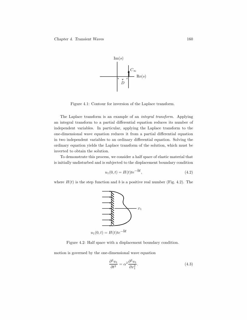
Chapter 4. Transient Waves 160
Re(s)
Im(s)
C∞
D
��
Figure 4.1: Contour for inversion of the Laplace transform.
The Laplace transform is an example of an integral transform. Applyingan integral transform to a partial differential equation reduces its number ofindependent variables. In particular, applying the Laplace transform to theone-dimensional wave equation reduces it from a partial differential equationin two independent variables to an ordinary differential equation. Solving theordinary equation yields the Laplace transform of the solution, which must beinverted to obtain the solution.
To demonstrate this process, we consider a half space of elastic material thatis initially undisturbed and is subjected to the displacement boundary condition
u1(0, t) = H(t)te−bt, (4.2)
where H(t) is the step function and b is a positive real number (Fig. 4.2). The
x1
u1(0, t) = H(t)te−bt�������
Figure 4.2: Half space with a displacement boundary condition.
motion is governed by the one-dimensional wave equation
∂2u1
∂t2= α2∂
2u1
∂x21
. (4.3)

Chapter 4. Transient Waves 161
To take the Laplace transform of this equation with respect to time, we multiplyit by e−st and integrate with respect to time from 0 to ∞:∫ ∞
0
∂2u1
∂t2e−st dt =
∫ ∞
0
α2 ∂2u1
∂x21
e−st dt. (4.4)
Integrating the term on the left side by parts, we obtain the expression∫ ∞
0
e−st ∂2u1
∂t2dt = e−st ∂u1
∂t
∣∣∣∣∞0
+ s
∫ ∞
0
e−st ∂u1
∂tdt. (4.5)
If we define the step function so that H(t) = 0 for t ≤ 0, the velocity ∂u1/∂t
is zero at t = 0. Because the inversion integral for the Laplace transform isevaluated along a contour for which Re(s) > 0 (Fig. 4.1), e−st → 0 as t → ∞.Evaluating the integral on the right side of Eq. (4.5) by parts, we obtain theresult ∫ ∞
0
e−st ∂2u1
∂t2dt = se−stu1
∣∣∣∞0
+ s2∫ ∞
0
e−stu1 dt.
We see that the left side of Eq. (4.4) assumes the form∫ ∞
0
∂2u1
∂t2e−st dt = s2
∫ ∞
0
u1e−st dt
= s2uL1 .
By using this expression, we can write Eq. (4.4) as
d2uL1
dx21
− s2
α2uL
1 = 0. (4.6)
The Laplace transform of the boundary condition, Eq. (4.2), with respect totime is
uL1 (0, s) =
∫ ∞
0
te−(b+ s)t dt =1
(b + s)2. (4.7)
We can write the solution of Eq. (4.6) in the form
uL1 = Aesx1/α + Be−sx1/α. (4.8)
Substituting this result into Eq. (4.1), we can see that the first term representsa wave propagating in the negative x1 direction. Thus we conclude that A = 0.From Eqs. (4.8) and (4.7), we find that
B =1
(b+ s)2,
so that the solution for the displacement is
u1 =1
2πi
∫C∞
1(b+ s)2
es(t − x1/α) ds. (4.9)

Chapter 4. Transient Waves 162
The Laplace transform is usually inverted by using one of the closed contoursshown in Fig. 4.3. We denote the straight vertical part of the contour by C1.The straight horizontal parts of the contour in Fig. 4.3.a are denoted by C2
and C4, and the semicircular part of the contours is denoted by C3.
(a)
Re(s)
Im(s)
Db
R C1
C2
C3
C4
� ����&
(b)
Re(s)
Im(s)
C1
C3
�
Figure 4.3: Closed contours in the complex s-plane.
If we denote the integrand in Eq. (4.9) by
g(s) =1
2πi(b+ s)2es(t − x1/α), (4.10)
the integral we must evaluate to determine the displacement is
u1 = limR→∞
∫C1
g(s) ds. (4.11)
The integral along the closed contour in Fig. 4.3.a can be expressed in terms ofthe residues of the integrand within the contour:
4∑k=1
∫Ck
g(s) ds = 2πi∑
Residues.
The integrand, Eq. (4.10), has a second-order pole at s = −b. From Eq. (A.13),the residue of the second-order pole is
lims→−b
d
ds[(s+ b)2g(s)] =
12πi
(t− x1
α
)e−b(t− x1/α).
We see that the limit of the integral over the closed contour as R → ∞ is
limR→∞
4∑k=1
∫Ck
g(s) ds =(t− x1
α
)e−b(t − x1/α). (4.12)

Chapter 4. Transient Waves 163
We can show that the integrals along C2 and C4 approach zero as R → ∞.On C2, s = x+ iR, where x ≤ D. Therefore, on C2∣∣∣es(t − x1/α)
∣∣∣ ≤ eD|t− x1/α|.
On C2, |b+ s| ≥ (R2 + b2)1/2, so∣∣(b+ s)2
∣∣ ≥ (R2 + b2). As a consequence,∣∣∣∣∫
C2
g(s) ds∣∣∣∣ ≤ eD|t− x1/α|
2π(R2 + b2)
∫C2
|ds| = DeD|t − x1/α|2π(R2 + b2)
.
From this expression we see that the integral along C2 vanishes as R → ∞.The same argument can be used to show that the integral along C4 vanishesas R → ∞.
To evaluate the integral along the semicircular contour C3, we use a resultcalled Jordan’s lemma:
Let CA denote a circular arc of radius R in the complex s-plane,and consider the integral
I =∫
CA
h(s)eas ds,
where h(s) is analytic on CA and a is a complex constant. Jordan’slemma states that if the maximum value of the magnitude of h(s)on CA approaches zero as R → ∞ and Re(as) ≤ 0 on CS , thenI → 0 as R→ ∞.
From Eq. (4.10), we see that on C3, Re[s(t − x1/α)] ≤ 0 when t > x1/α.Also, on C3 ∣∣∣∣ 1
2πi(b+ s)2
∣∣∣∣ ≤ 1(R− b)2
,
which approaches zero as R→ ∞. Therefore Jordan’s lemma states that
limR→∞
∫C3
g(s) ds = 0 when t >x1
α.
From Eqs. (4.11) and (4.12), we obtain the solution for the displacement:
u1 =(t− x1
α
)e−b(t − x1/α) when t >
x1
α.
When t < x1/α, we can evaluate the displacement by using the closed con-tour shown in Fig. 4.3.b. In this case the contour does not contain the pole,so the integral over the closed contour is zero. Jordan’s lemma states that theintegral over C ′
3 vanishes as R→ ∞ when t < x1/α, so the displacement is
u1 = limR→∞
∫C1
g(s) ds = 0 when t <x1
α.
The time t = x1/α is the time at which the wave arrives at the position x1.

Chapter 4. Transient Waves 164
4.2 Fourier Transform
The Fourier transform of a function f(t) is defined by
fF (ω) =∫ ∞
−∞f(t)e−iωt dt, (4.13)
where ω is the transform variable. The Fourier transform fF (ω) can be invertedto recover the function f(t) through the expression
f(t) =12π
∫ ∞
−∞fF (ω)eiωt dω. (4.14)
These two equations are called the Fourier integral theorem.
Example
For comparison with the Laplace transform, we apply the Fourier transformto the example discussed in the previous section: an undisturbed half space issubjected to the displacement boundary condition
u1(0, t) = H(t)te−bt, (4.15)
where H(t) is the step function and b is a positive real number (Fig. 4.2).The motion is governed by the one-dimensional wave equation
∂2u1
∂t2= α2∂
2u1
∂x21
. (4.16)
To take the Fourier transform of this equation with respect to time, we multiplyit by e−iωt and integrate with respect to time from −∞ to ∞:∫ ∞
−∞
∂2u1
∂t2e−iωt dt =
∫ ∞
−∞α2∂
2u1
∂x21
e−iωt dt. (4.17)
Integrating the term on the left side by parts, we obtain the expression∫ ∞
−∞e−iωt ∂
2u1
∂t2dt = e−iωt ∂u1
∂t
∣∣∣∣∞−∞
+ iω
∫ ∞
−∞e−iωt ∂u1
∂tdt. (4.18)
Because the material is initially undisturbed, the velocity ∂u1/∂t is zero att = −∞. We assume that the velocity is zero at t = ∞. Evaluating the integralon the right side of Eq. (4.18) by parts, we obtain the result∫ ∞
−∞e−iωt ∂u1
∂tdt = e−iωtiωu1
∣∣∣∞−∞
− ω2
∫ ∞
−∞e−iωtu1 dt.

Chapter 4. Transient Waves 165
The displacement is zero at t = −∞ and we assume it is zero at t = ∞. Bydoing so, we obtain the left side of Eq. (4.17) in the form∫ ∞
−∞
∂2u1
∂t2e−iωt dt = −ω2
∫ ∞
−∞u1e
−iωt dt
= −ω2uF1 .
By using this expression, we can write Eq. (4.17) as
d2uF1
dx21
+ω2
α2uF
1 = 0. (4.19)
By using the Fourier transform, we have reduced the partial differential equa-tion, Eq. (4.16), to an ordinary equation. We also take the Fourier transform ofEq. (4.15) with respect to time:∫ ∞
−∞u1(0, t)e−iωt dt =
∫ ∞
−∞H(t)te−bte−iωt dt,
which we can write as
uF1 (0, ω) =
∫ ∞
0
te−(b + iω)t dt.
Evaluating the integral on the right yields the Fourier transformed boundarycondition:
uF1 (0, ω) =
1(b+ iω)2
. (4.20)
We now proceed to obtain the solution for uF1 . We write the solution of
Eq. (4.19) in the form
uF1 = Aeiωx1/α +Be−iωx1/α. (4.21)
Substituting this result into the inversion integral, Eq. (4.14), we obtain anexpression for the displacement:
u1 =12π
∫ ∞
−∞Aeiω(x1/α+ t) dω +
12π
∫ ∞
−∞Beiω(−x1/α+ t) dω. (4.22)
We see that the first term represents a wave propagating in the negative x1
direction and the second term represents a wave propagating in the positive x1
direction. Because the boundary condition can give rise only to a wave propa-gating in the positive x1 direction, we conclude that A = 0. From Eqs. (4.21)and (4.20), we find that
uF1 =
1(b+ iω)2
e−iωx1/α. (4.23)

Chapter 4. Transient Waves 166
Therefore Eq. (4.22) for the displacement assumes the form
u1 =∫ ∞
−∞
12π(b+ iω)2
eiω(t − x1/α) dω. (4.24)
This expression for the displacement is an integral with respect to a realvariable ω. However, to evaluate the integral it is convenient to let ω be acomplex variable. By doing so, we can interpret Eq. (4.24) as a contour integralalong the real axis from Re(ω) = −∞ to Re(ω) = +∞ (Fig. 4.4.a).
(a)
Re(ω)
Im(ω)
��
(b)
Re(ω)
Im(ω)
CS
CR
R b�
���&
�''
��
Figure 4.4: (a) Path along the real axis in the complex ω-plane. (b) A closedcontour.
Consider the closed contour shown in Fig. 4.4.b, where CR is the part of thecontour along the real axis and CS is the semicircular part of the contour. Ifwe denote the integrand in Eq. (4.24) by
g(ω) =1
2π(b+ iω)2eiω (t − x1/α), (4.25)
the integral we must evaluate to determine the displacement is
u1 = limR→∞
∫CR
g(ω) dω. (4.26)
The integral along the closed contour can be expressed in terms of the residuesof the integrand within the contour:∫
CR
g(ω) dω +∫
CS
g(ω) dω = 2πi∑
Residues.
The integrand, Eq. (4.25), has a second-order pole at ω = bi. From Eq. (A.13),the residue of the second-order pole is
limω→bi
d
dω[(ω − bi)2g(ω)] =
12πi
(t− x1
α
)e−b(t− x1/α).

Chapter 4. Transient Waves 167
Therefore we find that the integral along the closed contour is∫CR
g(ω) dω +∫
CS
g(ω) dω =(t− x1
α
)e−b(t− x1/α).
This result is independent of R. Therefore, the limit of the integral over theclosed contour as R→ ∞ is
limR→∞
[∫CR
g(ω) dω +∫
CS
g(ω) dω]
=(t− x1
α
)e−b(t− x1/α). (4.27)
By using Jordan’s lemma (page 163), it is easy to show that
limR→∞
∫CS
g(ω) dω = 0 when t >x1
α.
Therefore, from Eqs. (4.26) and (4.27), we obtain the solution for the displace-ment:
u1 =(t− x1
α
)e−b(t − x1/α) when t >
x1
α. (4.28)
Notice that t = x1/α is the time at which the wave arrives at the position x1.
Fourier superposition and impulse response
If we know the solution of a problem with a steady-state boundary condition, wecan (in principle) use the Fourier transform to determine the solution of the sameproblem with a transient boundary condition. This powerful and commonlyused procedure is called Fourier superposition. Suppose that a problem has asteady-state boundary condition represented by the expression h(x)eiωt, whereh(x) may depend on position but not time, and let the resulting steady-statesolution of the problem be represented by g(x, ω)eiωt . Our objective is todetermine the solution for a transient boundary condition h(x)f(t), where f(t)is some prescribed function of time.
Let fF (ω) be the Fourier transform of f(t). For a given value of ω, ifwe multiply the steady-state boundary condition by (1/2π)fF (ω), obtaining(1/2π)fF (ω)h(x)eiωt , the resulting steady-state solution is (1/2π)fF (ω)g(x, ω)eiωt .(Notice that this is true only if the governing equations are linear.) Integratingthe boundary condition with respect to frequency from −∞ to ∞, we obtainthe transient boundary condition,
12π
∫ ∞
−∞fF (ω)h(x)eiωt dω = h(x)f(t),
and (again because the governing equations are linear), the solution is
12π
∫ ∞
−∞fF (ω)g(x, ω)eiωt dω. (4.29)

Chapter 4. Transient Waves 168
This is Fourier superposition; by integrating, we have superimposed steady-state solutions to obtain the solution of the transient problem. Notice that theproduct fF (ω)g(x, ω) is the Fourier transform of the transient solution.
Now suppose that f(t) is a delta function, f(t) = δ(t). This transient bound-ary condition is called an impulse, and the resulting solution is the impulseresponse. The Fourier transform of f(t) is
fF (ω) =∫ ∞
−∞δ(t)e−iωt dt = 1,
so that the Fourier transform of the transient solution is
fF (ω)g(x, ω) = g(x, ω).
The Fourier transform of the transient solution resulting from an impulse bound-ary condition equals the complex amplitude of the steady-state solution. Thefunction g(x, ω) is the impulse response in the frequency domain and its inverseis the impulse response in the time domain. This result has important impli-cations from both computational and experimental points of view: by applyingan impulse boundary condition, the steady state solution can be obtained as afunction of frequency.
As an example, we apply Fourier superposition to the problem discussed inthe previous section. We considered a half space subjected to a transient dis-placement boundary condition u1(0, t) = H(t)te−bt (Fig. 4.5.a). This boundary
x1
u1(0, t) = H(t)te−bt
(a)
�������
x1
u1(0, t) = eiωt
(b)
�������
Figure 4.5: (a) Half space subjected to a transient boundary condition. (b) Thecorresponding steady-state problem.
condition is of the form h(x)f(t) with h(x) = 1 and f(t) = H(t)te−bt. Wemust first solve the problem for the steady-state boundary condition u1(0, t) =

Chapter 4. Transient Waves 169
h(x)eiωt = eiωt (Fig. 4.5.b). The result is
u1(x1, t) = eiω(t − x1/α) = e−x1/αeiωt,
so the steady-state solution is of the form g(x, ω)eiωt with g(x, ω) = e−x1/α.The next step is to determine the Fourier transform of f(t):
fF (ω) =∫ ∞
−∞H(t)te−bte−iωt dt
=1
(b+ iω)2.
Substituting our expressions for g(x, ω) and fF (ω) into Eq. (4.29), we obtainthe transient solution
u1 =∫ ∞
−∞
12π(b+ iω)2
eiω (t − x1/α) dω, (4.30)
which is identical to Eq. (4.24). Thus Fourier superposition gives the same resultobtained by applying the Fourier transform to the transient problem. The taskof inverting the transform, evaluating the integral in Eq. (4.30), remains. Aswe saw in the previous section, analytical evaluation of such integrals is difficulteven in simple cases. We discuss efficient computational methods for evaluatingthem in the next section.
Notice that if the half-space in this example is subjected to an impulseboundary condition, u1(0, t) = δ(t), the Fourier transform of the transient solu-tion is
fF (ω)g(x, ω) = (1)(e−x1/α
)= e−x1/α,
which is the complex amplitude of the steady-state solution.
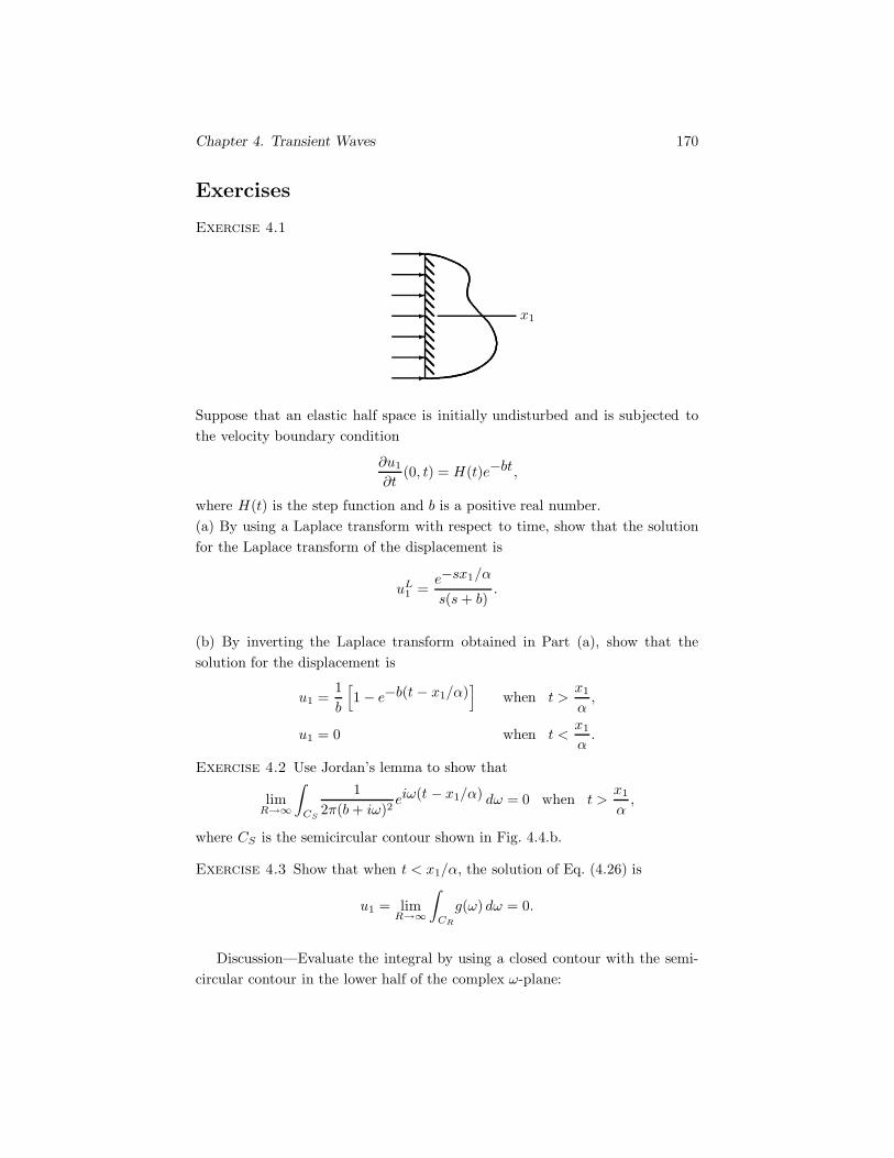
Chapter 4. Transient Waves 170
Exercises
Exercise 4.1
x1
�������
Suppose that an elastic half space is initially undisturbed and is subjected tothe velocity boundary condition
∂u1
∂t(0, t) = H(t)e−bt,
where H(t) is the step function and b is a positive real number.(a) By using a Laplace transform with respect to time, show that the solutionfor the Laplace transform of the displacement is
uL1 =
e−sx1/α
s(s+ b).
(b) By inverting the Laplace transform obtained in Part (a), show that thesolution for the displacement is
u1 =1b
[1 − e−b(t − x1/α)
]when t >
x1
α,
u1 = 0 when t <x1
α.
Exercise 4.2 Use Jordan’s lemma to show that
limR→∞
∫CS
12π(b+ iω)2
eiω(t − x1/α) dω = 0 when t >x1
α,
where CS is the semicircular contour shown in Fig. 4.4.b.
Exercise 4.3 Show that when t < x1/α, the solution of Eq. (4.26) is
u1 = limR→∞
∫CR
g(ω) dω = 0.
Discussion—Evaluate the integral by using a closed contour with the semi-circular contour in the lower half of the complex ω-plane:

Chapter 4. Transient Waves 171
Re(ω)
Im(ω)
C ′S
CR
R(
(()
�
��
��
Exercise 4.4 Suppose that an unbounded elastic material is subjected to theinitial displacement and velocity fields
u1(x1, 0) = p(x1),
∂u1
∂t(x1, 0) = 0,
where p(x1) is a prescribed function. By taking a Fourier transform with respectto x1 with the transform variable denoted by k, show that the solution for theFourier transform of the displacement is
uF1 = 1
2pF
(e−iαkt + eiαkt
),
where pF is the Fourier transform of the function p(x1).Discussion—To determine the solution for the displacement, it is not necessary
to invert the Fourier transform. By substituting the expression for uF1 into the
inversion integral, you obtain
u1 =12π
∫ ∞
−∞12p
F eik(x1 − αt) dk
+12π
∫ ∞
−∞12pF eik(x1 + αt) dk.
You can see by inspection of this expression that
u1 = 12p(x1 − αt) + 1
2p(x1 + αt).
Chapter 4. Transient Waves 172
4.3 Discrete Fourier Transform
The exponential form of the Fourier series of a function of time f(t) over theinterval 0 ≤ t ≤ T is
f(t) =∞∑
n=−∞Ane
iωnt, (4.31)
where the discrete frequencies ωn are
ωn = 2πn/T. (4.32)
The terms in this series are called the frequency components of f(t). Thisrepresentation is periodic over the interval T :
f(t + T ) = f(t).
By multiplying Eq. (4.31) by e−iωmt, integrating from t = 0 to t = T , andusing the orthogonality condition∫ T
0
eiωnte−iωmtdt ={
0 m �= n,T m = n,
(4.33)
we obtain an expression for the coefficients Am in terms of f(t):
Am =1T
∫ T
0
f(t)e−iωmtdt. (4.34)
In general, these coefficients are complex. A graph of their magnitudes as afunction of the frequencies ωm is called the frequency spectrum of f(t).
We divide the time interval T into an even numberN of intervals of length Δ,so that T = NΔ. Let the value of f(t) at some time within the nth interval bedenoted by fn, n = 0, 1, 2, . . . , N − 1. In terms of these samples of the functionf(t), we can approximate Eq. (4.34) by
Am = fDFm , (4.35)
where
fDFm =
1N
N−1∑n=0
fne−2πimn/N . (4.36)
The array fDFm , m = 0, 1, 2, . . . , N − 1, is called the discrete Fourier transform
of the discrete function fn. It converts the N time-domain samples fn into Nfrequency-domain samples fDF
n . Evaluation of this equation for m = n + N
shows that the fDFn are periodic over the interval N :
fDFn+N = fDF
n . (4.37)

Chapter 4. Transient Waves 173
Comparison of Eq. (4.34) to Eq. (4.13) shows that the Fourier transform of thesampled function f(t) is related to the discrete Fourier transform by
fF (ωn) = TfDFn . (4.38)
A function f(t) that has a finite Fourier series representation over a timeinterval 0 ≤ t ≤ T is said to be band-limited on that interval. That is, such afunction has a maximum frequency in its Fourier series. The truncated Fourierseries
f(t) =N/2−1∑
n=−N/2
Aneiωnt, (4.39)
whereωn = 2πn/NΔ, (4.40)
is an exact representation of a band-limited function f(t) in the interval 0 ≤t ≤ T provided the frequency ωN/2 = 2π/(2Δ) is greater than the maximumfrequency in the Fourier series of f(t). This connection between the samplinginterval and the exact representation of band-limited functions is called thesampling theorem, and ωN/2 is called the Nyquist frequency.
By using the periodicity condition, Eq. (4.37), together with Eqs. (4.35) and(4.39), it can be shown that
fm =N−1∑n=0
fDFn e2πinm/N , (4.41)
which is the inverse discrete Fourier transform. Thus Eqs. (4.36) and (4.41) areanalogous to the Fourier transform and its inverse, Eqs. (4.13) and (4.14). Thedifference is that the discrete Fourier transform is defined in terms of a functionwith a discrete domain.
Data are often obtained at discrete values of time, and in such cases thediscrete Fourier transform and its inverse can be applied in the same way theFourier transform and its inverse are applied to functions defined on continuousdomains. Because the discrete transform and its inverse can easily be evaluatedby computer, even when we deal with continuous, or analog data, it is oftenadvantageous to sample it at discrete times (a process called analog-to-digitalconversion) and use the discrete transform.
According to the sampling theorem, there is a one-to-one relation between aband-limited function f(t) and its discrete samples fn if the sampling interval Δis chosen so that at least two samples occur within each period of the maximumfrequency in the spectrum of f(t). Of course this is not possible if a function

Chapter 4. Transient Waves 174
is not band-limited, but in such cases it may be acceptable to approximate thefunction by one that is band limited.
When the transform or its inverse is computed as indicated in Eqs. (4.36)and (4.41), the amount of computation is proportional to N2. When N is apower of 2, a sequence of computations can be chosen so that only N log2N
operations are required. This procedure is called the fast Fourier transform, orFFT. For example, when N = 214 = 16384, the FFT algorithm is 1170 timesfaster. This algorithm has become the most important computational algorithmin digital electronics and signal processing, and is contained in many types ofcommercial software.
Examples
1. Half space with displacement boundary condition In Section 4.2, weapply the Fourier transform to a half space of elastic material subjected to thedisplacement boundary condition
u(0, t) = H(t)te−bt,
where H(t) is the step function and b is a constant. By taking Fourier transformsof the governing wave equation and the boundary condition, we obtain theFourier transform of the displacement field. The result, Eq. (4.23), is
uF =1
(b+ iω)2e−iωx1/α. (4.42)
We can begin with this expression and use the inverse discrete Fourier transformto obtain the displacement field u.
Applying the inverse FFT algorithm to this example results in a sequenceof N real numbers representing the displacement atN discretely spaced intervalsof time and at one position x1. These times are separated by the samplinginterval Δ, and it is up to us to specify not only the number of points N butalso Δ and the position x1.
The solution we want to approximate is a transient function whose amplitudeis significant only over a finite range of time. However, the solution obtainedwith the algorithm is periodic with period NΔ. While we are free to specify anyvalues for N and Δ, the quality of our results suffers if we make bad choices.For example, if Δ is too large, we cannot resolve the profile of the transientwave from the discrete solution. But selecting a very small value for Δ causesanother difficulty. The period of the FFT results, and consequently the “timewindow” within which we can view the results, is given by the product NΔ.

Chapter 4. Transient Waves 175
Therefore the choice of a small value for Δ must be offset by a large value of N ,which results in large computation times.
For the present example, we can choose a value of Δ based on the functionalform of the boundary condition. To obtain sufficient resolution of the transientwave, we select a sampling interval such that the quantity bΔ is small. Thisensures that the part of the propagating wave that is of significant amplitudeis sampled by a suitable number of points. Next, we select N large enoughto obtain a time window beginning at t = 0 sufficiently long to “capture” thesolution.
Let the discrete values of the displacement be um. The relation betweenthe time t and the index m is m = t/Δ. For convenience, we introduce theparameters
r = 1/bΔ,n = x1/αΔ.
We obtain uDFm (n) from Eqs. (4.38), (4.40), and (4.42):
buDFm (n) =
⎧⎪⎪⎨⎪⎪⎩
b
TuF (nαΔ, ωm) =
e−2πimn/N
bT (1 + 2πimr/N)2, −N/2 < m < N/2,
0, m = N/2.(4.43)
The function uF (x1, ω) is non-zero for all frequencies. However, its ampli-tude decreases monotonically with frequency, and we can approximate uF (x1, ω)by uDF
m (n) if its magnitude at the Nyquist frequency is small compared to itsmagnitude at zero frequency:∣∣∣∣ uF (x1, 0)
uF (x1, ωN/2)
∣∣∣∣ = |(1 + iπr)2| 1. (4.44)
This requires that r be large or, equivalently, that bΔ be small. This requirementwas satisfied by our choice of the sampling interval Δ.
For a given value of the nondimensional position n, we obtain uDFm (n) from
Eq. (4.43) and employ the inverse FFT algorithm to determine um(n). Theresulting solution for the displacement obtained with Δ = 1/b is compared tothe exact solution in Fig. 4.6. Only the portion of the time window 0 ≤ m ≤ N
is shown. Even with this coarse sampling, the discrete solution approximates theactual displacement. By decreasing the sampling interval Δ by a factor of 10,we obtain the comparison shown in Fig. 4.7. The discrete and exact solutionsare indistinguishable.

Chapter 4. Transient Waves 176
90 95 100 105 110−0.1
−0.05
0
0.05
0.1
0.15
0.2
0.25
0.3
0.35
0.4
m = t/Δ
Displacement×
b
Exact solution
FFT
Exact solution
FFT
Figure 4.6: Exact and FFT solutions for N = 256, r = 1, and n = 100.

Chapter 4. Transient Waves 177
50 100 150 200−0.1
−0.05
0
0.05
0.1
0.15
0.2
0.25
0.3
0.35
0.4
m = t/Δ
Displacement×
b
Exact solution
FFT
Exact solution
FFT
Figure 4.7: Exact and FFT solutions for N = 1024, r = 10, and n = 100.

Chapter 4. Transient Waves 178
2. Half-space with embedded layer If the impulse response of a problemis known, its Fourier transform is the solution of the corresponding steady-state problem. Here we demonstrate this procedure by obtaining the steady-state solution for a half space containing a layer of higher-impedance material(Fig. 4.8). We determine the impulse response by the method of characteristics,applying the procedure described in Section 2.7.
x1 = 0
x1
300αaΔ 50αaΔ
10αbΔ
$$$
$$$$
$$$
$$
$$$
$$
$$$
$$
$$$
$$$$$$
$$$
$$
Figure 4.8: Elastic half space with an embedded layer.
The compressional wave velocities in the half space and the layer are denotedby αa and αb, respectively, the densities are ρa and ρb, and the ratio of acousticimpedances is zb/za = 3. To apply the method of characteristics, we select atime increment Δ for the calculation that divides the portion of the half space tothe left of the embedded layer into 300 sublayers and the embedded layer itselfinto 10 sublayers. We divide the portion of the half space to the right of theembedded layer into 50 sublayers and impose a condition at the right boundarythat prevents the reflection of waves (see page 104).
The method of characteristics solution is evaluated at integer values of timem = t/Δ. We apply an impulse in velocity at the left boundary:
vm ={N m = 00 0 < m ≤ N − 1 ,
and terminate the calculation at m = N − 1. (In the subsequent application ofthe FFT algorithm, N is the size of the FFT array.) The velocity calculatedat the right “boundary” of the half-space using N = 1024 is shown in Fig. 4.9.It consists of a sequence of impulses with diminishing amplitude separated intime by 20Δ, the time required for an impulse to complete two transits acrossthe thickness of the embedded layer.
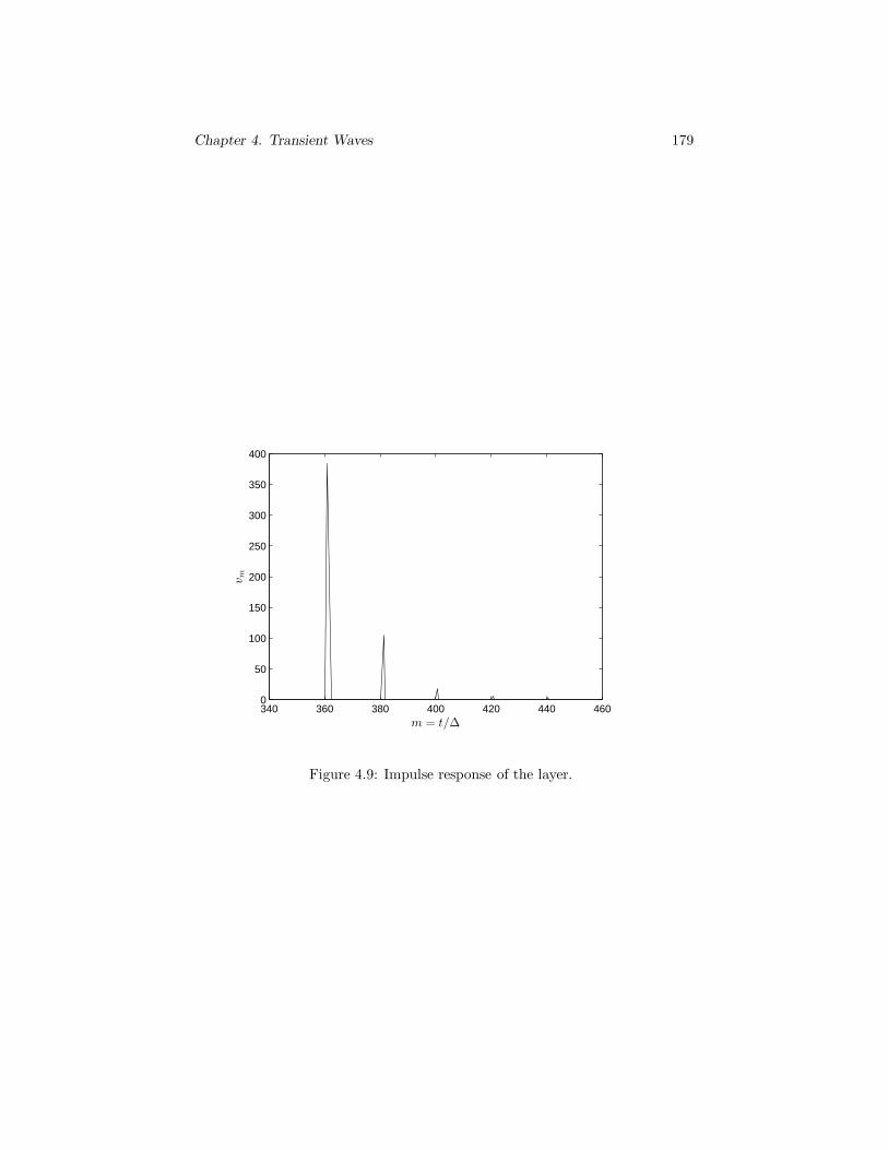
Chapter 4. Transient Waves 179
340 360 380 400 420 440 4600
50
100
150
200
250
300
350
400
m = t/Δ
v m
Figure 4.9: Impulse response of the layer.
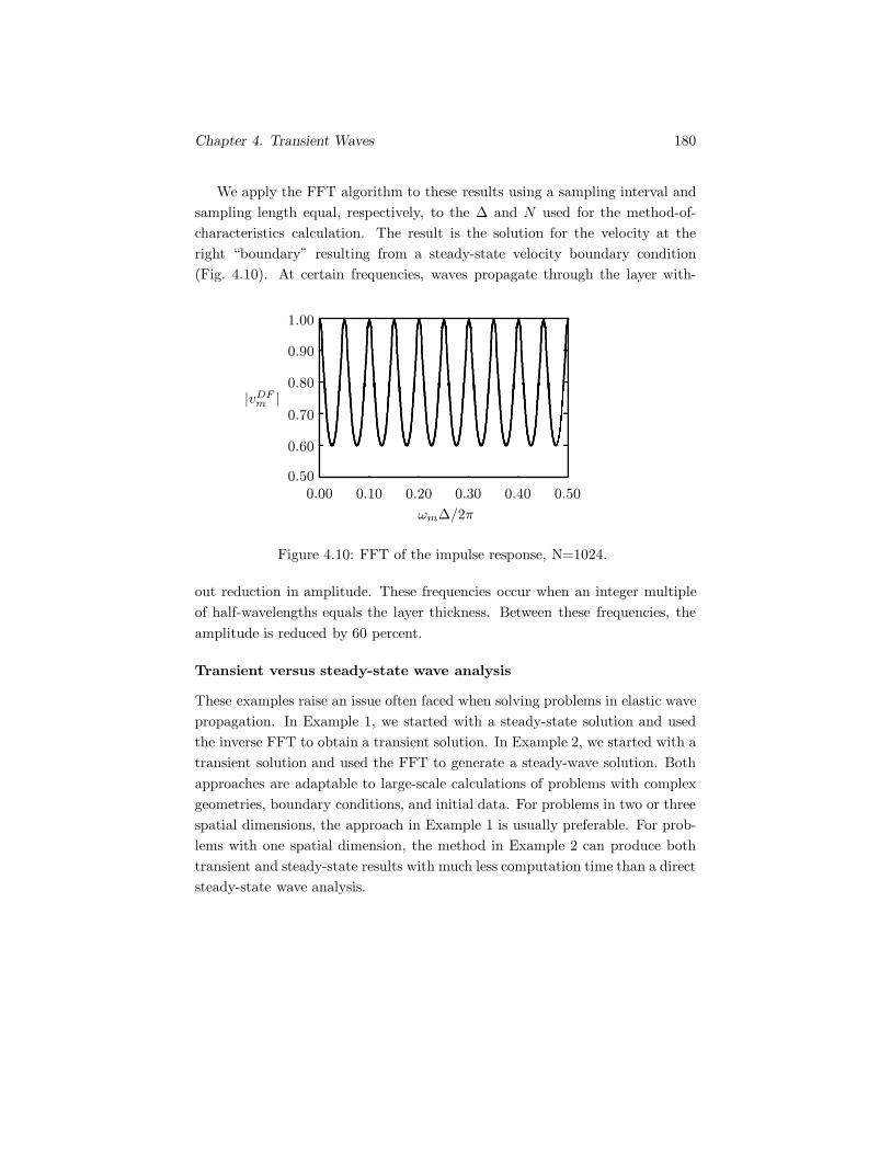
Chapter 4. Transient Waves 180
We apply the FFT algorithm to these results using a sampling interval andsampling length equal, respectively, to the Δ and N used for the method-of-characteristics calculation. The result is the solution for the velocity at theright “boundary” resulting from a steady-state velocity boundary condition(Fig. 4.10). At certain frequencies, waves propagate through the layer with-
ωmΔ/2π
|vDFm |
0.00 0.10 0.20 0.30 0.40 0.500.50
0.60
0.70
0.80
0.90
1.00
Figure 4.10: FFT of the impulse response, N=1024.
out reduction in amplitude. These frequencies occur when an integer multipleof half-wavelengths equals the layer thickness. Between these frequencies, theamplitude is reduced by 60 percent.
Transient versus steady-state wave analysis
These examples raise an issue often faced when solving problems in elastic wavepropagation. In Example 1, we started with a steady-state solution and usedthe inverse FFT to obtain a transient solution. In Example 2, we started with atransient solution and used the FFT to generate a steady-wave solution. Bothapproaches are adaptable to large-scale calculations of problems with complexgeometries, boundary conditions, and initial data. For problems in two or threespatial dimensions, the approach in Example 1 is usually preferable. For prob-lems with one spatial dimension, the method in Example 2 can produce bothtransient and steady-state results with much less computation time than a directsteady-state wave analysis.

Chapter 4. Transient Waves 181
Exercises
Exercise 4.5 Consider the function of time f(t) = t.(a) If you represent this function as a discrete Fourier series
f(t) =∞∑
n=−∞Ane
iωnt
over the interval 0 ≤ t ≤ 1, show that the coefficients are
An =e−iωn (iωn + 1)
ω2n
− 1ω2
n
. (4.45)
(b) Show that A0 = 1/2.Discussion—To do part (b), express the term e−iωn as a Taylor series.
Exercise 4.6 Calculate the results shown in Fig. 4.6. Use T = 100 and α = 1.Repeat the calculation using N =256, 128, and 64. What causes the solutionto change?
Discussion—In carrying out these computations, you need to be aware thatcommercial implementations of the FFT vary. Some are specialized to realvalues of fn, but some accept complex values. The particular implementationused influences the choice of N . Another variation is the placement of thenormalization factor 1/N ; it can appear in Eq. (4.36) or in Eq. (4.41), with acorresponding affect on Eq. (4.43).
Exercise 4.7 In Exercise 4.6, assume that there is a second boundary at adistance x1 = L = 200αΔ from the existing boundary. Assuming the materialis fixed at the new boundary, derive the finite Fourier transform of the displace-ment field.
Discussion—Accounting for the new boundary requires new expressions forthe constants A and B in Eq. (4.21).
Exercise 4.8 The discrete Fourier transform converts N real numbers into Ncomplex numbers. Use the properties of periodicity and symmetry of fDF
n toshow that half of the values of the fDF
n are sufficient to determine the otherhalf.

Chapter 4. Transient Waves 182
4.4 Transient Waves in Dispersive Media
In Chapter 3 we demonstrated that steady-state longitudinal waves in an elasticlayer and steady-state waves in layered materials are dispersive: the phase ve-locity depends on the frequency of the wave. Dispersive waves commonly occurin problems involving boundaries and interfaces. The Fourier integral theoremexpresses a transient wave in terms of superimposed steady-state componentswith a spectrum of frequencies. If there is dispersion, each component prop-agates with the phase velocity corresponding to its frequency. As a result, atransient wave tends to spread, or disperse, as it propagates. This is the originof the term dispersion. Because the different frequency components propagatewith different velocities, it is not generally possible to define a velocity of atransient wave. However, we will show that a transient wave having a narrowfrequency spectrum propagates with a velocity called the group velocity.
Group velocity
Let us consider waves propagating in the positive x1 direction, and suppose thatthe phase velocity c1(ω) = ω/k1(ω) depends on frequency. First we consider asteady-state wave with frequency ω0:
f(x1, t) = Aei[ω0t− k1(ω0)x1] = Aeiω0ξ(ω0), (4.46)
whereξ(ω) = t− k1(ω)x1
ω= t− x1
c1(ω).
Its Fourier transform is
fF (x1, ω) = 2πAe−ik1(ω0)x1δ(ω − ω0),
which you can confirm using the Fourier integral
f(x1, t) =12π
∫ ∞
−∞fF (x1, ω)eiωt dω. (4.47)
Thus the frequency “spectrum” is a single frequency (Fig. 4.11.a).We now consider a narrow, uniform frequency spectrum (a narrow-band spec-
trum) centered about the frequency ω0 (Fig. 4.11.b):
fF (x1, ω) =
⎧⎨⎩
πA
Ωe−ik1(ω)x1 −Ω ≤ ω − ω0 ≤ Ω,
0 otherwise,(4.48)

Chapter 4. Transient Waves 183
ω
∣∣fF (x, ω)∣∣
ω0
(a)
ω
∣∣fF (x, ω)∣∣
ω0
πA
Ω
(b)
2Ω� �
.........................................................
Figure 4.11: (a) Spectrum of a wave with a single frequency ω0. (b) Spectrumof a narrow-band wave.
where Ω is a constant. We assume Ω to be sufficiently small that we can ap-proximate the wave number by retaining only the first-order term in its Taylorseries expansion:
k1(ω) = k1(ω0) +dk1
dω(ω0)(ω − ω0) = k1(ω0) +
ω
cg(ω0), (4.49)
where we defineω = ω − ω0
andcg(ω) =
dω
dk1. (4.50)
Substituting Eqs. (4.48) and (4.49) into Eq. (4.47), we obtain the time-domainexpression for the narrow-band wave:
f(x1 , t) = Aeiω0ξ(ω0) sin[Ωξg(ω0)]Ωξg(ω0)
, (4.51)
whereξg(ω) = t− x1
cg(ω). (4.52)
Notice that when Ω → 0, Eq. (4.51) reduces to Eq. (4.46), which describes awave with frequency ω0 propagating at the phase velocity c1(ω0). The wavedescribed by Eq. (4.46) is called the phase wave.
The terms ξ(ω0) and ξg(ω0) in Eq. (4.51) are D’Alembert independent vari-ables associated with forward propagating waves. Thus this equation is theproduct of two waves: the phase wave, propagating with the phase veloc-ity c1(ω0), and a group wave propagating with the group velocity cg(ω0). In

Chapter 4. Transient Waves 184
Fig. 4.12, we plot Eq. (4.51) for x = 0 and ω0 = 20Ω. The very short-wavelengthphase wave is “enveloped” by the group wave. The group wave characterizesthe gross shape and propagation velocity of the transient wave. The velocity
Figure 4.12: Phase wave (—) and group wave (−−) with ω0 = 20Ω.
of the phase wave relative to the group wave is determined by the dispersioncurve relating ω to k1 (Fig. 4.13). When the curve is concave upward, the phasewave propagates more slowly than the group wave. An observer stationary withrespect to the group wave sees phase waves being “created” at the front of thegroup wave, traveling backwards, and disappearing at the back. When the curveis straight, the phase wave and group wave move together. When the curve isconcave downward, the observer sees phase waves being created at the back ofthe group wave, moving forward, and disappearing at the front.
In Fig. 4.14, we compare the phase and group velocities of the first modefor longitudinal waves in an elastic layer for Poisson’s ratio ν = 0.3. (SeeSection 3.5). The group velocity is approximately equal to the phase velocityat very low frequency, but is smaller than the phase velocity at all frequencies.At high frequency, both the phase and group velocities approach the Rayleighwave velocity.
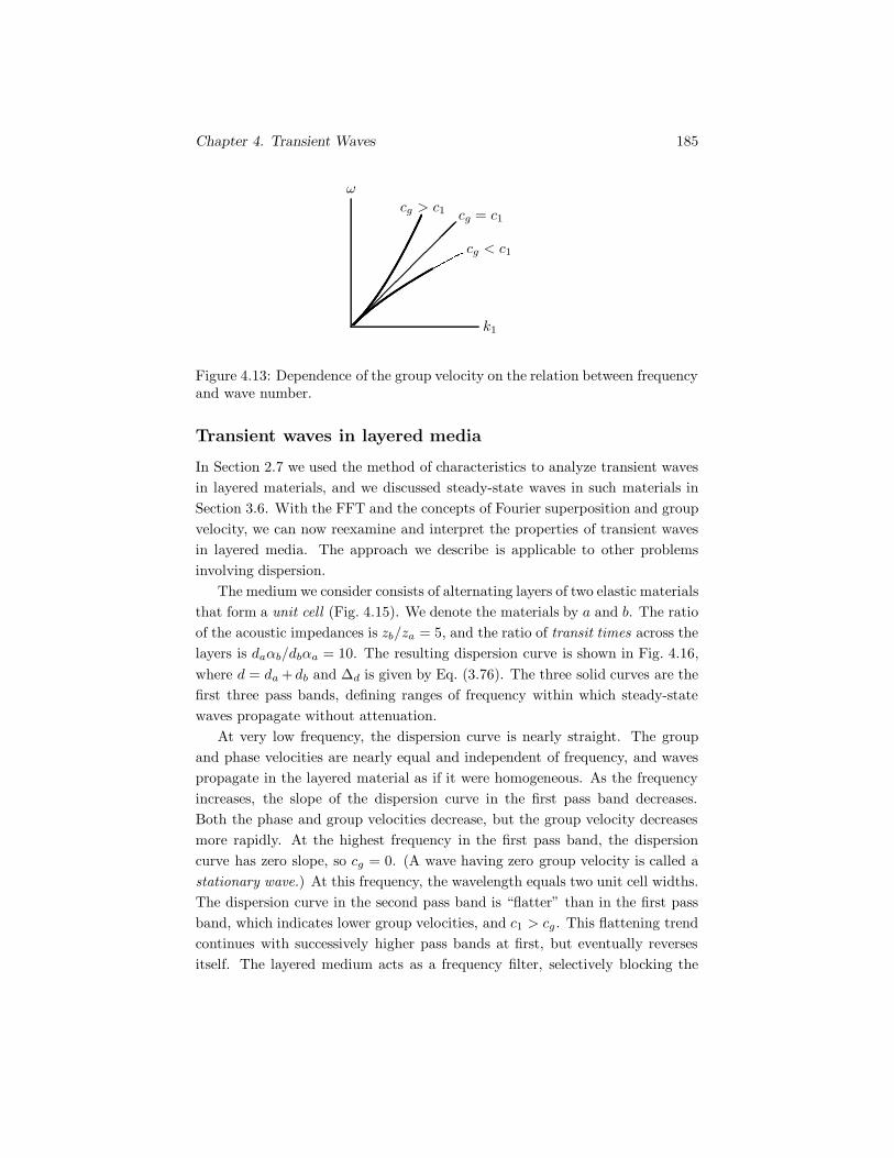
Chapter 4. Transient Waves 185
cg = c1
cg < c1
cg > c1
k1
ω
��������
Figure 4.13: Dependence of the group velocity on the relation between frequencyand wave number.
Transient waves in layered media
In Section 2.7 we used the method of characteristics to analyze transient wavesin layered materials, and we discussed steady-state waves in such materials inSection 3.6. With the FFT and the concepts of Fourier superposition and groupvelocity, we can now reexamine and interpret the properties of transient wavesin layered media. The approach we describe is applicable to other problemsinvolving dispersion.
The medium we consider consists of alternating layers of two elastic materialsthat form a unit cell (Fig. 4.15). We denote the materials by a and b. The ratioof the acoustic impedances is zb/za = 5, and the ratio of transit times across thelayers is daαb/dbαa = 10. The resulting dispersion curve is shown in Fig. 4.16,where d = da + db and Δd is given by Eq. (3.76). The three solid curves are thefirst three pass bands, defining ranges of frequency within which steady-statewaves propagate without attenuation.
At very low frequency, the dispersion curve is nearly straight. The groupand phase velocities are nearly equal and independent of frequency, and wavespropagate in the layered material as if it were homogeneous. As the frequencyincreases, the slope of the dispersion curve in the first pass band decreases.Both the phase and group velocities decrease, but the group velocity decreasesmore rapidly. At the highest frequency in the first pass band, the dispersioncurve has zero slope, so cg = 0. (A wave having zero group velocity is called astationary wave.) At this frequency, the wavelength equals two unit cell widths.The dispersion curve in the second pass band is “flatter” than in the first passband, which indicates lower group velocities, and c1 > cg . This flattening trendcontinues with successively higher pass bands at first, but eventually reversesitself. The layered medium acts as a frequency filter, selectively blocking the

Chapter 4. Transient Waves 186
0 1 2 3 4 5 6 7 80
0.2
0.4
0.6
0.8
1
1.2
1.4
1.6
1.8
2
ωh
β
cRβ
c1β
cgβ
Figure 4.14: First-mode phase and group velocities for symmetric longitudinalwaves in a layer of thickness 2h.

Chapter 4. Transient Waves 187
x1
d
da db
��
�� ��
unit cell
$$$$$$$$
$$$$$$$$
$$
$$$$
$$$$$$$$$$
$$$$$$$$$$$$$$
Figure 4.15: Medium of alternating layers of elastic materials a and b.
Figure 4.16: Dispersion relation for a layered medium.

Chapter 4. Transient Waves 188
propagation of steady-state components with frequencies within stop bands.Within a given pass band, the dispersion increases with frequency. Within eachpass band, the group velocity varies from zero at the “edges” to a maximumvalue near the center.
With these observations in mind, we examine two types of waves. By sub-jecting the layered medium to an impulse boundary condition, we obtain a wavehaving a broad spectrum of frequencies. We then apply a boundary conditionresulting in a wave with a narrow frequency spectrum. We obtain the solu-tions for the transient waves by a simple modification of the program given onpage 106, dividing a into 10 sublayers and treating b as a single layer. As aresult, Eq. (3.76) gives Δ2
d = 153Δ2.
Impulse boundary condition For the first calculation, the velocity on theleft boundary is 1 at t = 0 and zero thereafter. The velocity of the layeredmedium at the left boundary of layer 71 is shown in Fig. 4.17. The results show
Figure 4.17: Impulse response at a point in the layered medium.
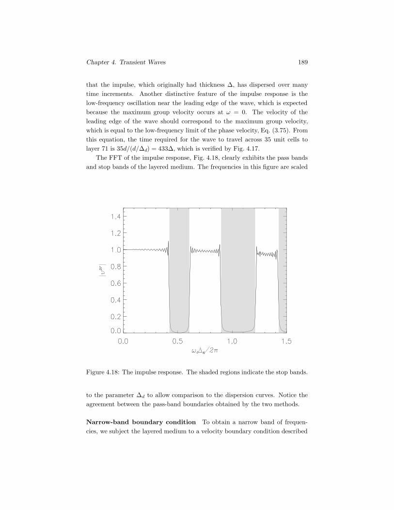
Chapter 4. Transient Waves 189
that the impulse, which originally had thickness Δ, has dispersed over manytime increments. Another distinctive feature of the impulse response is thelow-frequency oscillation near the leading edge of the wave, which is expectedbecause the maximum group velocity occurs at ω = 0. The velocity of theleading edge of the wave should correspond to the maximum group velocity,which is equal to the low-frequency limit of the phase velocity, Eq. (3.75). Fromthis equation, the time required for the wave to travel across 35 unit cells tolayer 71 is 35d/(d/Δd) = 433Δ, which is verified by Fig. 4.17.
The FFT of the impulse response, Fig. 4.18, clearly exhibits the pass bandsand stop bands of the layered medium. The frequencies in this figure are scaled
Figure 4.18: The impulse response. The shaded regions indicate the stop bands.
to the parameter Δd to allow comparison to the dispersion curves. Notice theagreement between the pass-band boundaries obtained by the two methods.
Narrow-band boundary condition To obtain a narrow band of frequen-cies, we subject the layered medium to a velocity boundary condition described
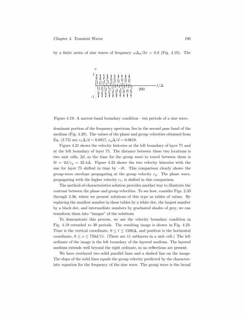
Chapter 4. Transient Waves 190
by a finite series of sine waves of frequency ωΔd/2π = 0.8 (Fig. 4.19). The
t/Δ
v
200
1
-1
Figure 4.19: A narrow-band boundary condition—ten periods of a sine wave.
dominant portion of the frequency spectrum lies in the second pass band of themedium (Fig. 4.20). The values of the phase and group velocities obtained fromEq. (3.73) are c1Δ/d = 0.0817, cgΔ/d = 0.0618.
Figure 4.21 shows the velocity histories at the left boundary of layer 71 andat the left boundary of layer 75. The distance between these two locations istwo unit cells, 2d, so the time for the group wave to travel between them isδt = 2d/cg = 32.4Δ. Figure 4.22 shows the two velocity histories with theone for layer 75 shifted in time by −δt. This comparison clearly shows thegroup-wave envelope propagating at the group velocity cg. The phase wave,propagating with the higher velocity c1, is shifted in this comparison.
The method-of-characteristics solution provides another way to illustrate thecontrast between the phase and group velocities. To see how, consider Figs. 2.33through 2.36, where we present solutions of this type as tables of values. Byreplacing the smallest number in these tables by a white dot, the largest numberby a black dot, and intermediate numbers by graduated shades of grey, we cantransform them into “images” of the solutions.
To demonstrate this process, we use the velocity boundary condition inFig. 4.19 extended to 30 periods. The resulting image is shown in Fig. 4.23.Time is the vertical coordinate, 0 ≤ t ≤ 1500Δ, and position is the horizontalcoordinate, 0 ≤ x ≤ 750d/11. (There are 11 sublayers in a unit cell.) The leftordinate of the image is the left boundary of the layered medium. The layeredmedium extends well beyond the right ordinate, so no reflections are present.
We have overlayed two solid parallel lines and a dashed line on the image.The slope of the solid lines equals the group velocity predicted by the character-istic equation for the frequency of the sine wave. The group wave is the broad

Chapter 4. Transient Waves 191
Figure 4.20: Frequency spectrum of the boundary condition superimposed onthe pass bands (light areas) and stop bands (shaded areas) of the medium.
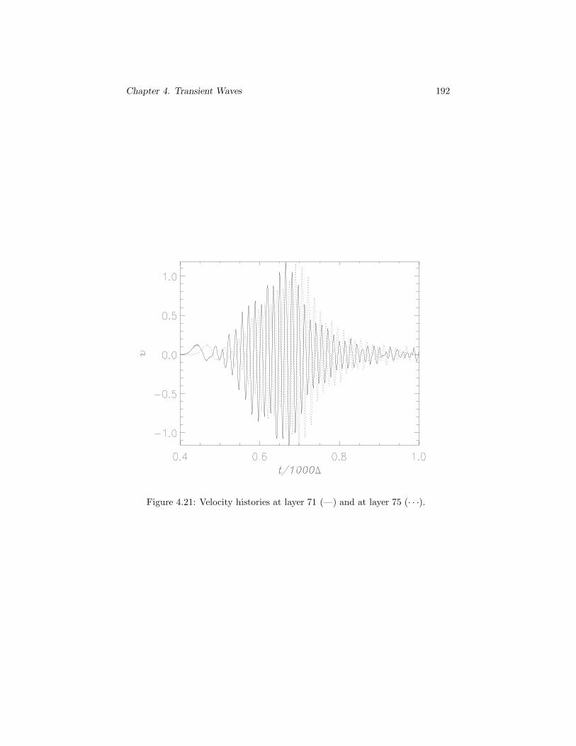
Chapter 4. Transient Waves 192
Figure 4.21: Velocity histories at layer 71 (—) and at layer 75 (· · ·).

Chapter 4. Transient Waves 193
Figure 4.22: The time history at layer 71 (—) compared to the time-shiftedhistory at layer 75 (· · ·).

Chapter 4. Transient Waves 194
Figure 4.23: Image of the transient wave.

Chapter 4. Transient Waves 195
grey band contained between these lines. The slope of the dashed line equalsthe phase velocity. The propagation of the phase wave appears in the pattern aslines parallel to the dashed line. The phase wave travels faster then the groupwave, appearing at the back edge of the group and disappearing at the frontedge.
Exercises
Exercise 4.9 Show that the group velocity cg = dω/dk is related to the phasevelocity c1 by
cg = c1 + k1dc1dk1
=c1
1 − ω
c1
dc1dω
.
Exercise 4.10 In Section 3.5, we analyzed acoustic waves in a channel.(a) Show that the group velocity of such waves is related to the phase velocityby cgc1 = α2.(b) What is the maximum value of the group velocity?
Answer: (b) α.
Exercise 4.11 Use Eq. (3.73) to derive an expression for the group velocity ofa layered medium with periodic layers.
Exercise 4.12 Use the result of Exercise 4.11 to show that the group velocityis zero at the edges of a pass band.

Chapter 4. Transient Waves 196
4.5 Cagniard-de Hoop Method
This integral transform method has yielded solutions to many important tran-sient problems in elastic wave propagation. We will demonstrate the procedureby obtaining the solution to a transient problem known as Lamb’s problem.
Let us consider a half space of elastic material that is initially stationary. Leta cartesian coordinate system be oriented with the x1-x2 plane coincident withthe boundary of the half space and the x3 axis extending into the material. Weassume that at t = 0 the boundary of the half space is subjected to the stressboundary condition
[T33]x3=0 = −T0H(t)δ(x1),
where T0 is a constant, H(t) is the step function, and δ(x1) is a Dirac deltafunction (Fig. 4.24.a). Thus at t = 0 the half space is subjected to a uniformline load along the x2 axis (Fig. 4.24.b).
(a)
x1
x3
T33 = −T0H(t)δ(x1)
� x1
x2
x3
T33 = −T0H(t)δ(x1)
(b)
��
��
����
����
����������
................................
Figure 4.24: Elastic half space subjected to a uniform line load along the x2
axis.
From the boundary condition we see that no motion occurs in the x2 direc-tion. The motion is described by the displacement field
u1 = u1(x1, x3, t),
u3 = u3(x1, x3, t).
For this displacement field, the expressions for the stress components T33 and T13
in terms of displacements are
T33 = λ∂u1
∂x1+ (λ + 2μ)
∂u3
∂x3.
T13 = μ
(∂u1
∂x3+∂u3
∂x1
),
(4.53)
Chapter 4. Transient Waves 197
In terms of the Helmholtz decomposition
u = ∇φ+ ∇× ψ,
the displacement components u1 and u3 are expressed by
u1 =∂φ
∂x1− ∂ψ
∂x3, u3 =
∂φ
∂x3+∂ψ
∂x1, (4.54)
where ψ is the x2 component of the vector potential ψ. Using these expressions,we can write Eqs. (4.53) in terms of the potentials φ and ψ:
T13 = μ
(2
∂2φ
∂x1∂x3+∂2ψ
∂x21
− ∂2ψ
∂x23
),
T33 = λ∂2φ
∂x21
+ (λ + 2μ)∂2φ
∂x23
+ 2μ∂2ψ
∂x1∂x3.
(4.55)
The potentials φ and ψ are governed by the wave equations
∂2φ
∂t2= α2
(∂2φ
∂x21
+∂2φ
∂x23
),
∂2ψ
∂t2= β2
(∂2ψ
∂x21
+∂2ψ
∂x23
). (4.56)
By using Eqs. (4.55), we can write the stress boundary conditions in terms of φand ψ: [
λ∂2φ
∂x21
+ (λ + 2μ)∂2φ
∂x23
+ 2μ∂2ψ
∂x1∂x3
]x3=0
= −T0H(t)δ(x1),[2
∂2φ
∂x1∂x3+∂2ψ
∂x21
− ∂2ψ
∂x23
]x3=0
= 0.(4.57)
The Laplace transforms of the potentials φ and ψ with respect to time aredefined by
φL =∫ ∞
0
φe−st dt, ψL =∫ ∞
0
ψe−st dt.
We take the Laplace transforms of Eqs. (4.56),
s2φL = α2
(∂2φL
∂x21
+∂2φL
∂x23
), s2ψL = β2
(∂2ψL
∂x21
+∂2ψL
∂x23
), (4.58)
and also take the Laplace transforms of the boundary conditions, eqs(4.57):[λ∂2φL
∂x21
+ (λ+ 2μ)∂2φL
∂x23
+ 2μ∂2ψL
∂x1∂x3
]x3=0
= −T0δ(x1)s
,[2∂2φL
∂x1∂x3+∂2ψL
∂x21
− ∂2ψL
∂x23
]x3=0
= 0.(4.59)

Chapter 4. Transient Waves 198
The next step is the key to the Cagniard-de Hoop method. We define Fouriertransforms of φL and ψL with respect to x1 by
φLF =∫ ∞
−∞φLe−iksx1 dx1, ψLF =
∫ ∞
−∞ψLe−iksx1 dx1.
Notice that in place of the usual transform variable, we use the product of aparameter k and the Laplace transform variable s. The corresponding inversionintegrals are
φL =12π
∫ ∞
−∞sφLF eiksx1 dk, ψL =
12π
∫ ∞
−∞sψLF eiksx1 dk. (4.60)
Using these definitions, we take the Fourier transforms of Eqs. (4.58) and writethe resulting equations in the forms
d2φLF
dx23
− (k2 + v2P )s2φLF = 0,
d2ψLF
dx23
− (k2 + v2S)s2ψLF = 0,
(4.61)
where vP and vS are the compressional and shear slownesses defined by vP =1/α, vS = 1/β. We also take the Fourier transform of the boundary conditions,Eqs. (4.59), obtaining[
−k2s2λφLF + (λ+ 2μ)d2φLF
dx23
+ 2μiksdψLF
dx3
]x3=0
= −T0
s,[
2iksdφLF
dx3− k2s2ψLF − d2ψLF
dx23
]x3=0
= 0.(4.62)
The solutions of Eqs. (4.61) are
φLF = Ae−(k2 + v2P )1/2sx3+Be(k
2 + v2P )1/2sx3 ,
ψLF = Ce−(k2 + v2S)1/2sx3+De(k
2 + v2S)1/2sx3 .
(4.63)
Substituting these expressions into the inversion integral for the Laplace trans-form, we can see that the terms containingA and C represent waves propagatingin the positive x3 direction and the terms containing B and D represent wavespropagating in the negative x3 direction. Because the boundary conditions donot give rise to waves propagating in the negative x3 direction, we concludethat B = 0 and D = 0. Substituting Eqs. (4.63) into the boundary conditions,Eqs. (4.62), we obtain two equations we can solve for A and C:
A =−T0(2k2 + v2
S)s3μQ
, C =T02ik(k2 + v2
P )1/2
s3μQ,

Chapter 4. Transient Waves 199
where Q is defined by
Q = (2k2 + v2S)2 − 4k2(k2 + v2
P )1/2(k2 + v2S)1/2.
(In obtaining these expressions we have used the relation (λ + 2μ)v2P = μv2
S .)Substituting these expressions for A and C into Eqs. (4.63), we obtain thesolutions for the transformed potentials φLF and ψLF :
φLF =−T0(2k2 + v2
S)s3μQ
e−(k2 + v2P )1/2sx3 ,
ψLF =T02ik(k2 + v2
P )1/2
s3μQe−(k2 + v2
S)1/2sx3 .
We substitute these expressions into the Fourier inversion integrals, Eqs. (4.60),to obtain the solutions for the transformed potentials φL and ψL:
φL = − 12π
∫ ∞
−∞
T0(2k2 + v2S)
s2μQe−[(k2 + v2
P )1/2x3 − ikx1]s dk,
ψL =12π
∫ ∞
−∞
T02ik(k2 + v2P )1/2
s2μQe−[(k2 + v2
S)1/2x3 − ikx1]s dk.
By using these two results and Eq. (4.55), we obtain the solution for the Laplacetransform of the stress component T33 in the form of the sum of two terms:
TL33 = (TL
33)1 + (TL33)2 =
∫ ∞
−∞g1(k) dk +
∫ ∞
−∞g2(k) dk, (4.64)
where
g1(k) = −T0(2k2 + v2S)2
2πQe−[(k2 + v2
P )1/2x3 − ikx1]s,
g2(k) =2T0k
2(k2 + v2S)1/2(k2 + v2
P )1/2
πQe−[(k2 + v2
S)1/2x3 − ikx1]s.
Our objective is to determine the stress component T33 by inverting theLaplace transforms (TL
33)1 and (TL33)2. (The other components of stress can be
determined by procedures similar to the one we use to determine T33.) Theseterms are expressed in terms of integrals along the real axis of the complex k-plane. The Cagniard-de Hoop method involves changing the integration contourin the complex k-plane in such a way that the integrals assume the form of thedefinition of the Laplace transform. By doing so, the terms (T33)1 and (T33)2can be determined directly.

Chapter 4. Transient Waves 200
Evaluation of (T33)1
To make the integral (TL33)1 assume the form of the definition of the Laplace
transform, we define a real parameter t by the expression
t = (k2 + v2P )1/2x3 − ikx1.
We can write this equation in the form
(x21 + x2
3)k2 − 2itx1k + v2
Px23 − t2 = 0. (4.65)
We introduce polar coordinates r, θ in the x1-x3 plane (Fig. 4.25), so that
x1 = r cos θ, x3 = r sin θ.
In terms of r and θ, we can write Eq. (4.65) as
x1
x3
r����
Figure 4.25: Polar coordinates r, θ in the x1-x3 plane.
r2k2 − 2itrk cos θ + v2P r
2 sin2 θ − t2 = 0.
The solutions of this equation for k are
k± =it
rcos θ ±
(t2
r2− v2
P
)1/2
sin θ. (4.66)
As the value of the parameter t goes from vP r to ∞, the values of k given bythis equation describe the two paths in the complex k-plane shown in Fig. 4.26,starting from the point (vP cos θ)i and approaching the asymptotes shown inthe figure.
Consider the closed contour in the complex k-plane shown in Fig. 4.27. Thesolution k+ describes the path labeled B+ and the solution k− describes thepath labeled B−. The contour consists of a straight portion C1 along the realaxis from −R to R, closed by two circular arcs C2 and C3 and two portionsalong the contours B+ and B−. Our goal is to express the integral (TL
33)1in terms of integrals along the contours B+ and B− by applying the Cauchy

Chapter 4. Transient Waves 201
Re(k)
Im(k)
B+B− }vP cos θ((((((
���
���
���
� ��*���
Figure 4.26: The two paths B+ and B− in the complex k-plane.
integral theorem to the closed contour. Before we can apply the Cauchy integraltheorem, we must determine the poles and branch points of g1(k).
The function g1(k) has branch points at k = ±vP i and at k = ±vS i. The onlypoles of the integrand are the zeros of the function Q. If we set k = i/cR in thefunction Q, the equation Q = 0 becomes identical to the Rayleigh characteristicequation, Eq. (3.50). Therefore two of the zeros of Q are k = ±i/cR, where cR isthe Rayleigh wave velocity. We define the Rayleigh wave slowness by vR = 1/cRand write these zeros of Q as k = ±vRi. These poles are not within the closedcontour. We show these branch points and poles of g1(k) in Fig. 4.28, and alsoshow suitable branch cuts to make g1(k) single-valued. The branch points andpoles shown in Fig. 4.28 are not within the closed contour shown in Fig. 4.27,and the contour does not cross the branch cuts. Therefore, we can apply theCauchy integral theorem to the closed contour:∫
C1
g1(k) dk +∫
C2
g1(k) dk+∫
C3
g1(k) dk
−∫
B+
g1(k) dk +∫
B−g1(k) dk = 0.
(4.67)
The reason for the minus sign on the integral along B+ is that the integral isevaluated in the direction shown in Fig. 4.27. The integral (TL
33)1 is
(TL33)1 = lim
R→∞
∫C1
g1(k) dk.
The integrals along the circular contours C2 and C3 vanish as R→ ∞. Therefore

Chapter 4. Transient Waves 202
Re(k)
Im(k)
B+B−
C1
C2C3
R−R
��*
��
���
��+ ,
Figure 4.27: Closed contour in the complex k-plane.
Eq. (4.67) states that
(TL33)1 = lim
R→∞
[∫B+
g1(k) dk−∫
B−g1(k) dk
].
By using the Cauchy integral theorem, we have expressed the integral (TL33)1
in terms of integrals along the contours shown in Fig. 4.26. We express theseintegrals in terms of the parameter t by making a change of variable:
(TL33)1 =
∫ ∞
vP r
g1(k+)∂k+
∂tdt−
∫ ∞
vP r
g1(k−)∂k−∂t
dt.
Recall that k+ and k− are the values of k on B+ and B−. By introducing a stepfunction H(t− vP r), we can change the lower limits of the integrals to zero:
(TL33)1 =
∫ ∞
0
H(t− vP r)g1(k+)∂k+
∂tdt−
∫ ∞
0
H(t− vP r)g1(k−)∂k−∂t
dt.
We substitute the explicit expressions for the integrands g1(k+) and g1(k−) intothis equation, obtaining the result
(TL33)1 = −T0
2π
∫ ∞
0
H(t− vP r)(2k2
+ + v2S)2
Q+
∂k+
∂te−st dt
+T0
2π
∫ ∞
0
H(t− vP r)(2k2
− + v2S)2
Q−
∂k−∂t
e−st dt,(4.68)
where Q+ and Q− indicate that the function Q is expressed in terms of k+
and k−.

Chapter 4. Transient Waves 203
Re(k)
Im(k)
vP i
vS i
vRi
−vP i
−vS i
−vRi
���
���
�
��
Figure 4.28: Poles and branch points of the function g1(k) and branch cuts tomake it single-valued.
This completes the application of the Cagniard-de Hoop method to theterm (TL
33)1. The terms on the right of Eq. (4.68) have the form of the definitionof the Laplace transform: the transform variable s does not appear anywhereexcept in the exponential term. Therefore we conclude that the term (T33)1 is
(T33)1 =T0
2πH(t − vP r)
{−
(2k2+ + v2
S)2
Q+
∂k+
∂t+
(2k2− + v2
S)2
Q−
∂k−∂t
}. (4.69)
Because k+ and k− are known as functions of position and time, Eq. (4.66), thisis a closed-form solution for the term (T33)1.
Evaluation of (T33)2
To make the integral (TL33)2 in Eq. (4.64) assume the form of the definition of
the Laplace transform, we define the real parameter t by
t = (k2 + v2S)1/2x3 − ikx1.
In terms of the polar coordinates r, θ, the solutions of this equation for k are
k± =it
rcos θ ±
(t2
r2− v2
S
)1/2
sin θ. (4.70)

Chapter 4. Transient Waves 204
As the value of the parameter t goes from vSr to ∞, the values of k given bythis equation describe the two paths in the complex k-plane shown in Fig. 4.29,starting from the point (vS cos θ)i and approaching the asymptotes shown inthe figure. The solution k+ describes the path labeled B+ and the solution k−describes the path labeled B−.
Re(k)
Im(k)
B+B− }vS cos θ((((((
���
���
���
� ��*���
Figure 4.29: The two paths B+ and B− in the complex k-plane.
The branch points and poles of g2(k) are identical to the branch points andpoles of the integrand g1(k) of T 1L
33 . They are shown in Fig. 4.28 together withbranch cuts that make g2(k) single valued. In this case, when we constructthe closed contour in the k-plane along the contours B+ and B−, the contourintersects the imaginary axis above the branch point k = vP i when vS cos θ > vP
(Fig 4.30). We therefore modify the closed contour so that it goes around thebranch cut by introducing two branch-line contours L+ and L−.
As the value of the parameter t goes from vSr to ∞, the functions k± givenby Eq. (4.70) describe the paths B+ and B− in the k-plane. We can also usethe function k− to describe the branch-line contours L+ and L−. We write k−in the form
k− =it
rcos θ − i
(v2
S − t2
r2
)1/2
sin θ.
When t = vSr, k− = (vS cos θ)i. As t decreases below the value vSr, we cansee that the value of k− moves downward along the imaginary axis, that is, itmoves along the branch-line contours L+ and L−. To determine the value of tfor which k− reaches the bottom of the branch-line contours, we set k− = vP i

Chapter 4. Transient Waves 205
Re(k)
Im(k)
vP i
vS i
vRi
−vP i
−vS i
−vRi
L+L−
B+B−
C1
C2C3
R−R
���
���
�
��
������*���
��+ ,
��
Figure 4.30: Closed contour in the complex k-plane that goes around the branchcut.
and solve for t. We denote the result by t:
t = r[vP cos θ + (v2S − v2
P )1/2 sin θ]. (4.71)
Thus as the value of the parameter t goes from t to vSr, the function k− describesthe paths L+ and L−.
We can apply the Cauchy integral theorem to the closed contour shown inFig. 4.30: ∫
C1
g2(k) dk +∫
C2
g2(k) dk+∫
C3
g2(k) dk
−∫
B+
g2(k) dk +∫
B−g2(k) dk
−∫
L+
g2(k) dk +∫
L−g2(k) dk = 0.
(4.72)
The reason for the minus sign on the integrals along B+ and L+ is that weevaluate the integrals in the directions shown in Fig. 4.30. The integral (TL
33)2is
(TL33)2 = lim
R→∞
∫C1
g2(k) dk.
The integrals along the circular contours C2 and C3 vanish as R→ ∞. Therefore

Chapter 4. Transient Waves 206
Eq. (4.72) states that
(TL33)2 = lim
R→∞
[∫B+
g2(k) dk −∫
B−g2(k) dk +
∫L+
g2(k) dk −∫
L−g2(k) dk
].
We can express these integrals in terms of the parameter t by making a changeof variable:
(TL33)2 =
∫ ∞
vSr
g2(k+)∂k+
∂tdt−
∫ ∞
vSr
g2(k−)∂k−∂t
dt
+∫ vSr
t
[g2(k−)]L+
∂k−∂t
dt−∫ vSr
t
[g2(k−)]L−∂k−∂t
dt.
The subscripts L+ and L− mean that the function g2(k−) is to be evaluatedon the right and left sides of the branch cut. By introducing appropriate stepfunctions, we can make the limits of the integrals be from 0 to infinity:
(TL33)2 =
∫ ∞
0
H(t− vSr)g2(k+)∂k+
∂tdt−
∫ ∞
0
H(t− vSr)g2(k−)∂k−∂t
dt
+∫ ∞
0
H(vs cos θ − vP )H(t − t)H(vSr − t)[g2(k−)]L+
∂k−∂t
dt
−∫ ∞
0
H(vs cos θ − vP )H(t − t)H(vSr − t)[g2(k−)]L−∂k−∂t
dt.
We include the step function H(vs cos θ− vP ) in the last two terms because thebranch-line contours exist only when vs cos θ > vP . We substitute the explicitexpressions for the integrands g2(k+) and g2(k−) into this equation, obtainingthe result
(TL33)2 =
2T0
π
∫ ∞
0
H(t− vSr)k2+(k2
+ + v2S)1/2(k2
+ + v2P )1/2
Q+
∂k+
∂te−st dt
−2T0
π
∫ ∞
0
H(t− vSr)k2−(k2
− + v2S)1/2(k2
− + v2P )1/2
Q−
∂k−∂t
e−st dt
+2T0
π
∫ ∞
0
H(vs cos θ − vP )H(t − t)H(vSr − t)
[k2−(k2− + v2
S)1/2(k2− + v2P )1/2
Q−
∂k−∂t
]L+
e−st dt
−2T0
π
∫ ∞
0
H(vs cos θ − vP )H(t − t)H(vSr − t)
[k2−(k2− + v2
S)1/2(k2− + v2P )1/2
Q−
∂k−∂t
]L−
e−st dt,
where Q+ and Q− indicate that the function Q is expressed in terms of k+
and k−.
Chapter 4. Transient Waves 207
This completes the application of the Cagniard-de Hoop method to theterm (TL
33)2. The term (T33)2 is
(T33)2 =2T0
πH(t − vSr)
{k2+(k2
+ + v2S)1/2(k2
+ + v2P )1/2
Q+
∂k+
∂t
−k2−(k2− + v2
S)1/2(k2− + v2P )1/2
Q−
∂k−∂t
}
+2T0
πH(vs cos θ − vP )H(t − t)H(vSr − t)
⎧⎨⎩[k2−(k2− + v2
S)1/2(k2− + v2P )1/2
Q−
∂k−∂t
]L+
−[k2−(k2− + v2
S)1/2(k2− + v2P )1/2
Q−
∂k−∂t
]L−
⎫⎬⎭ .
(4.73)
Solution for T33
From Eqs. (4.69) and (4.73), the closed-form solution for the stress compo-nent T33 is
T33 = (T33)1 + (T33)2
=T0
2πH(t− vP r)
{−
(2k2+ + v2
S)2
Q+
∂k+
∂t+
(2k2− + v2S)2
Q−∂k−∂t
}
+2T0
πH(t− vSr)
{k2+(k2
+ + v2S)1/2(k2
+ + v2P )1/2
Q+
∂k+
∂t
−k2−(k2− + v2
S)1/2(k2− + v2P )1/2
Q−
∂k−∂t
}
+2T0
πH(vs cos θ − vP )H(t − t)H(vSr − t)
⎧⎨⎩[k2−(k2− + v2
S)1/2(k2− + v2P )1/2
Q−
∂k−∂t
]L+
−[k2−(k2
− + v2S)1/2(k2
− + v2P )1/2
Q−
∂k−∂t
]L−
⎫⎬⎭ .
The first term in the solution (the term containing the step functionH(t − vP r)) is a disturbance that propagates with the compressional wave ve-locity α (Fig. 4.31). The second term (the term containing the step functionH(t− vSr)) is a disturbance that propagates with the shear wave speed β. Thewavefront that moves with the compressional wave speed causes a secondarydisturbance at the surface that propagates with the shear wave speed, shown asthe cross hatched area shown in Fig. 4.31. This disturbance is the third termof the solution, which originates from the branch-line integrals.
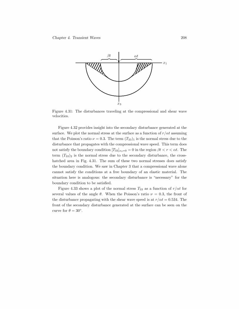
Chapter 4. Transient Waves 208
x1
x3
βt︷ ︸︸ ︷ αt︷ ︸︸ ︷&
������
--
--
--
Figure 4.31: The disturbances traveling at the compressional and shear wavevelocities.
Figure 4.32 provides insight into the secondary disturbance generated at thesurface. We plot the normal stress at the surface as a function of r/αt assumingthat the Poisson’s ratio ν = 0.3. The term (T33)1 is the normal stress due to thedisturbance that propagates with the compressional wave speed. This term doesnot satisfy the boundary condition [T33]x3=0 = 0 in the region βt < r < αt. Theterm (T33)2 is the normal stress due to the secondary disturbance, the cross-hatched area in Fig. 4.31. The sum of these two normal stresses does satisfythe boundary condition. We saw in Chapter 3 that a compressional wave alonecannot satisfy the conditions at a free boundary of an elastic material. Thesituation here is analogous: the secondary disturbance is “necessary” for theboundary condition to be satisfied.
Figure 4.33 shows a plot of the normal stress T33 as a function of r/αt forseveral values of the angle θ. When the Poisson’s ratio ν = 0.3, the front ofthe disturbance propagating with the shear wave speed is at r/αt = 0.534. Thefront of the secondary disturbance generated at the surface can be seen on thecurve for θ = 30◦.

Chapter 4. Transient Waves 209
0 0.1 0.2 0.3 0.4 0.5 0.6 0.7 0.8 0.9 1−0.4
−0.3
−0.2
−0.1
0
0.1
0.2
0.3
0.4
(T33)2/T0
(T33)1/T0
r/αt
Figure 4.32: The normal stresses at the boundary for Poisson’s ratio ν = 0.3.

Chapter 4. Transient Waves 210
0 0.1 0.2 0.3 0.4 0.5 0.6 0.7 0.8 0.9 1−4
−3
−2
−1
0
1
2
3
θ = 0
θ = 30◦
θ = 60◦
θ = 90◦
r/αt
T33/T0
θ = 0
θ = 30◦
θ = 60◦
θ = 90◦
θ = 0
θ = 30◦
θ = 60◦
θ = 90◦
θ = 0
θ = 30◦
θ = 60◦
θ = 90◦
Figure 4.33: The normal stress T33 for Poisson’s ratio ν = 0.3.

Chapter 4. Transient Waves 211
Exercise
Exercise 4.13 Consider Lamb’s problem for an acoustic medium. (See thediscussion of an acoustic medium on page 44.) Use the Cagniard-de Hoopmethod to show that the solution for the stress component T33 is
T33 = −T0
πH
(t− r
α
) sin θ
r
(1 − r2
t2α2
)1/2.

Chapter 5
Nonlinear WavePropagation
To obtain the equations governing a linear elastic material, weassumed that the stresses in the material were linear functions ofthe strains and that derivatives of the displacement were sufficientlysmall that higher-order terms could be neglected. In large-amplitudewaves, such as those created by high-velocity impacts or explosions,these assumptions are violated, and the equations governing the be-havior of the material are nonlinear. In this chapter we discuss thetheory of nonlinear wave propagation and apply it to a nonlinearelastic material. We derive the equations of one-dimensional non-linear elasticity and discuss the theory of characteristics for systemsof first-order hyperbolic equations in two independent variables. Wegive a brief introduction to the theory of singular surfaces and discussthe properties of shock and acceleration waves in elastic materials.
Materials subjected to large-amplitude waves do not usually be-have elastically. The stress generally depends upon the temperatureand the rate of change of the strain in addition to the strain. Nev-ertheless, we can demonstrate some of the qualitative features ofwaves of this type, and methods used to analyze them, using a non-linear elastic material as an example. The concluding discussion ofthe steady compressional waves and release waves observed in ex-perimental studies of large amplitude waves will not be limited toelastic materials.
212

Chapter 5. Nonlinear Wave Propagation 213
5.1 One-Dimensional Nonlinear Elasticity
Here we summarize the theory of one-dimensional nonlinear elasticity. We firstshow how the motion and strain of the material are described, then obtain theequations of motion from the postulates for conservation of mass and balance oflinear momentum without making approximations or assumptions of linearity.
Motion
To describe the one-dimensional motion of a material, we express the position ofa point of the material as a function of the time and its position in the referencestate:
x = x(X, t).
This equation gives the position at time t of the point of the material that wasat position X in the reference state (Fig. 5.1).
X x
x
�
Figure 5.1: The position X of the material in the reference state and the posi-tion x at time t.
The displacement and velocity fields are defined by
u = x(X, t) −X,
v =∂
∂tx(X, t).
Deformation gradient and longitudinal strain
Consider an element of material that has width dX in the reference state(Fig. 5.2). The width of this element at time t is
dx = x(X + dX, t) − x(X, t) = F dX, (5.1)

Chapter 5. Nonlinear Wave Propagation 214
where the termF =
∂x
∂X(5.2)
is called the deformation gradient.
X X + dX x x+ dx
x
dX dx
Figure 5.2: An element of the material in the reference state and at time t.
In this chapter we define the longitudinal strain of the material by
ε = −(dx− dX
dX
)= 1 − F. (5.3)
This definition, commonly used in studies of nonlinear waves in solids, is thenegative of the traditional definition of the strain. It is positive when the lengthof the element dX decreases. This definition is used because in experimentalstudies of nonlinear waves in solids the material is most often compressed, soit is convenient to use a definition of strain that is positive when the materialis in compression. We see from Eq. (5.3) that the deformation gradient F canalso be used as a measure of the longitudinal strain.
Conservation of mass
From Fig. 5.2, we see that conservation of mass requires that
ρ0dX = ρ dx,
where ρ is the density of the material and ρ0 is the density in the reference state.From Eq. (5.1), the deformation gradient is related to the density by
F =ρ0
ρ.

Chapter 5. Nonlinear Wave Propagation 215
We take the partial derivative of this equation with respect to time, obtainingthe expression
∂v
∂X= −ρ0
ρ2
∂ρ
∂t, (5.4)
where we use a hat ˆ to indicate that a variable is expressed in terms of thematerial, or Lagrangian, variables X, t. Using the chain rule, we can write theleft side of this equation as
∂v
∂X=
∂x
∂X
∂v
∂x= F
∂v
∂x=ρ0
ρ
∂v
∂x. (5.5)
We can also write the partial derivative of ρ(X, t) with respect to time as
∂ρ
∂t=∂ρ
∂t+∂ρ
∂xv,
where ρ is the spatial, or Eulerian representation for the density. Using thisexpression and Eq. (5.5), we can write Eq. (5.4) as
∂ρ
∂t+∂(ρv)∂x
= 0, (5.6)
which is the equation of conservation of mass for the material, Eq. (1.46).
Balance of linear momentum
Figure 5.3 shows the free-body diagram at time t of an element of material thathas width dX in the reference state. T is the normal stress.
X
dX
T T +∂T
∂XdX
� ��������
�������
Figure 5.3: Free-body diagram of an element of material.
Newton’s second law for the element is
ρ0 dX∂v
∂t=
(T +
∂T
∂XdX
)− T .
Chapter 5. Nonlinear Wave Propagation 216
Thus we obtain the equation of balance of linear momentum for the material inLagrangian form:
ρ0∂v
∂t=∂T
∂X. (5.7)
Applying the chain rule to the right side of this equation,
∂T
∂X=
∂x
∂X
∂T
∂x=ρ0
ρ
∂T
∂x,
and using the result∂v
∂t=∂v
∂t+∂v
∂xv,
we obtain the equation of balance of linear momentum in the spatial, or Eulerianform:
ρ
(∂v
∂t+∂v
∂xv
)=∂T
∂x. (5.8)
Stress-strain relation
To obtain a model for a nonlinear elastic material, we assume that the stress Tis a function of the deformation gradient:
T = T (F ). (5.9)
Lagrangian and Eulerian formulations
The material, or Lagrangian, form of the equation of balance of linear momen-tum is Eq. (5.7),
ρ0∂v
∂t=∂T
∂X.
Using Eq. (5.9), we can write the equation of balance of linear momentum as
ρ0∂v
∂t= TF
∂F
∂X, (5.10)
where TF = dT /dF . From the definition of the deformation gradient F , Eq. (5.2),we see that
∂F
∂t=
∂v
∂X. (5.11)
This completes the Lagrangian formulation of one-dimensional nonlinear elas-ticity. Equations (5.10) and (5.11) are two first-order differential equations inthe two dependent variables v and F . We can write these equations in thematrix form [
ρ0 00 1
] [vF
]t
+[
0 −TF
−1 0
] [vF
]X
= 0, (5.12)

Chapter 5. Nonlinear Wave Propagation 217
where the subscripts t and X denote partial derivatives.The spatial, or Eulerian form of the equation of balance of linear momentum,
Eq. (5.8), can be written
ρ
(∂v
∂t+∂v
∂xv
)= −∂p
∂x, (5.13)
where p = −T is the pressure. For an elastic material, the pressure is a functionof the longitudinal strain:
p = p(ε), (5.14)
whereε = 1 − ρ0
ρ. (5.15)
The motion of the material is also governed by the equation of conservation ofmass, Eq. (5.6):
∂ρ
∂t+∂(ρv)∂x
= 0. (5.16)
This completes the Eulerian formulation of one-dimensional nonlinear elastic-ity. Equations (5.13), (5.14), (5.15), and (5.16) are four equations in the fourdependent variables v, p, ε, and ρ.
5.2 Hyperbolic Systems and Characteristics
In Section 5.1 we showed that the equations governing one-dimensional nonlin-ear elasticity can be written as a system of first-order differential equations intwo independent variables, Eq. (5.12). Let us consider a generalization of thatsystem of equations:⎡⎢⎢⎢⎣a11 a12 · · · a1n
a21 a22 · · · a2n
......
...an1 an2 · · · ann
⎤⎥⎥⎥⎦⎡⎢⎢⎢⎣u1
u2
...un
⎤⎥⎥⎥⎦
t
+
⎡⎢⎢⎢⎣b11 b12 · · · b1n
b21 b22 · · · b2n
......
...bn1 bn2 · · · bnn
⎤⎥⎥⎥⎦⎡⎢⎢⎢⎣u1
u2
...un
⎤⎥⎥⎥⎦
x
= 0,
where the dependent variables u1, u2, . . . , un are functions of two independentvariables x, t. The subscripts t and x denote partial derivatives. We assumethat the coefficients a11, a12, . . . , ann and b11, b12, . . . , bnn may be functions ofthe dependent variables, but do not depend on derivatives of the dependentvariables. We write this system of equations as
Aut + Bux = 0. (5.17)
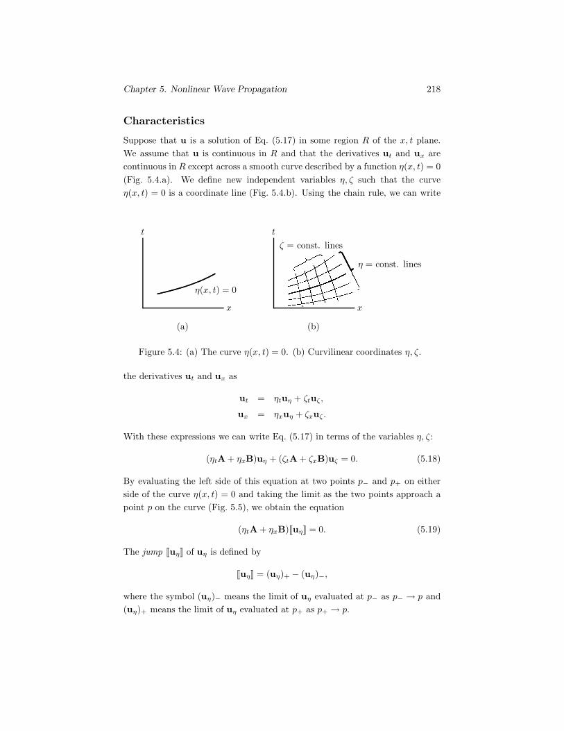
Chapter 5. Nonlinear Wave Propagation 218
Characteristics
Suppose that u is a solution of Eq. (5.17) in some region R of the x, t plane.We assume that u is continuous in R and that the derivatives ut and ux arecontinuous in R except across a smooth curve described by a function η(x, t) = 0(Fig. 5.4.a). We define new independent variables η, ζ such that the curveη(x, t) = 0 is a coordinate line (Fig. 5.4.b). Using the chain rule, we can write
(a)
x
t
η(x, t) = 0
(b)
x
t
η = const. lines
ζ = const. lines
Figure 5.4: (a) The curve η(x, t) = 0. (b) Curvilinear coordinates η, ζ.
the derivatives ut and ux as
ut = ηtuη + ζtuζ,
ux = ηxuη + ζxuζ .
With these expressions we can write Eq. (5.17) in terms of the variables η, ζ:
(ηtA + ηxB)uη + (ζtA + ζxB)uζ = 0. (5.18)
By evaluating the left side of this equation at two points p− and p+ on eitherside of the curve η(x, t) = 0 and taking the limit as the two points approach apoint p on the curve (Fig. 5.5), we obtain the equation
(ηtA + ηxB)[[uη]] = 0. (5.19)
The jump [[uη]] of uη is defined by
[[uη]] = (uη)+ − (uη)−,
where the symbol (uη)− means the limit of uη evaluated at p− as p− → p and(uη)+ means the limit of uη evaluated at p+ as p+ → p.
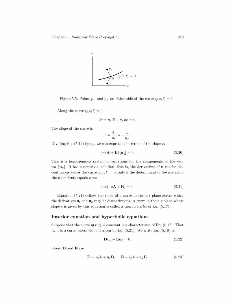
Chapter 5. Nonlinear Wave Propagation 219
x
t
p
p+
p−
η(x, t) = 0���""#
��!
Figure 5.5: Points p− and p+ on either side of the curve η(x, t) = 0.
Along the curve η(x, t) = 0,
dη = ηt dt+ ηx dx = 0.
The slope of the curve is
c =dx
dt= − ηt
ηx.
Dividing Eq. (5.19) by ηx, we can express it in terms of the slope c:
(−cA + B)[[uη]] = 0. (5.20)
This is a homogeneous system of equations for the components of the vec-tor [[uη]]. It has a nontrivial solution, that is, the derivatives of u can be dis-continuous across the curve η(x, t) = 0, only if the determinant of the matrix ofthe coefficients equals zero:
det(−cA + B) = 0. (5.21)
Equation (5.21) defines the slope of a curve in the x, t plane across whichthe derivatives ut and ux may be discontinuous. A curve in the x, t plane whoseslope c is given by this equation is called a characteristic of Eq. (5.17).
Interior equation and hyperbolic equations
Suppose that the curve η(x, t) = constant is a characteristic of Eq. (5.17). Thatis, it is a curve whose slope is given by Eq. (5.21). We write Eq. (5.18) as
Duη + Euζ = 0, (5.22)
where D and E are
D = ηtA + ηxB, E = ζtA + ζxB. (5.23)

Chapter 5. Nonlinear Wave Propagation 220
Equation (5.21) implies that the determinant of the matrix of D is zero. Becausethe determinant of a square matrix is equal to the determinant of its transpose,det(DT ) = 0. This is the necessary condition for the existence of a non-zerovector r such that
DT r = 0. (5.24)
The product of Eq. (5.22) with the transpose of r is
rTDuη + rTEuζ = 0. (5.25)
The first term in this equation is equal to zero as a consequence of Eq. (5.24):
rTDuη = uTη DT r = 0;
therefore Eq. (5.25) reduces to
rTEuζ = 0. (5.26)
This differential equation governs the variation of the solution u along a charac-teristic. It is called the interior equation, and is the foundation of the method ofcharacteristics. Dividing Eq. (5.24) by ηx, we obtain a more convenient equationfor determining the vector r:
(−cAT + BT )r = 0. (5.27)
When the roots of Eq. (5.21) are real and there are n real, linearly indepen-dent vectors r that satisfy Eq. (5.27) in a region R of the x, t plane, Eqs. (5.17)are said to be hyperbolic in R.
Examples
A first-order hyperbolic equation
Consider the first-order partial differential equation
∂u
∂t+ α
∂u
∂x= 0, (5.28)
where α = α(u) is a function of the dependent variable u. When α is a constant,it is easy to show that the solution of this differential equation is the D’Alembertsolution u = f(x − αt). When α depends on u, the differential equation isnonlinear. Although it is a very simple equation, its solution has some of thesame qualitative features exhibited by waves in nonlinear elastic materials.

Chapter 5. Nonlinear Wave Propagation 221
Equation 5.28 is of the form of Eq. (5.17). Because there is only one equation,the matrices reduce to scalars: A = 1 and B = α, and Eq. (5.21) for the slope cbecomes the scalar equation
−c(1) + α = 0.
Thus c = α = α(u), and we see that the slope of a characteristic depends onthe value of u.
We use the variable ζ in the interior equation, Eq. (5.26), to measure distancealong a characteristic. In this example we can simply let ζ = t. From Eq. (5.23),the scalar E = 1. Substituting the values of A and B into (5.27), it becomesthe scalar equation
[−c(1) + α]r = 0,
which is satisfied for any scalar r since c = α. As a result, the interior equationreduces to the scalar equation
uζ = 0.
Thus u is constant along a characteristic. Because the slopes of the character-istics depend only on u, the characteristics are straight lines.
Let us assume that the value of α(u) decreases monotonically with u (Fig. 5.6).Suppose that at t = 0, the value of u as a function of x has the distribution
Constant
Increases
Decreases
u
α(u)
Figure 5.6: The function α(u).
shown in Fig. 5.7.a. Thus we know the slopes of the characteristics c = α(u)at t = 0. This information is sufficient to determine the characteristics sincethey are straight lines (Fig. 5.7.b). The slopes dx/dt of the characteristics in-crease with increasing x because the initial distribution of u decreases withincreasing x. Because the value of u is constant along a characteristic, we canuse the characteristics to determine the solution at any time (Figs. 5.7.c, d,and e). The distribution of u as a function of x changes as a function of time;the wave “spreads” with increasing time.
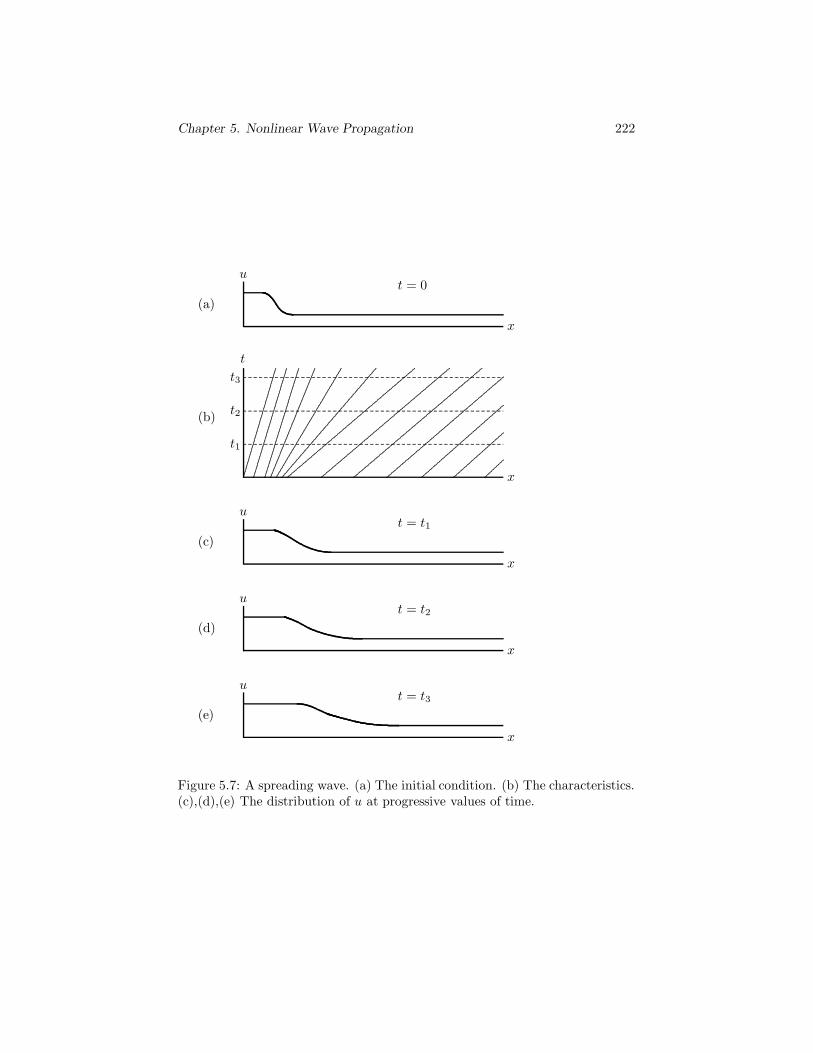
Chapter 5. Nonlinear Wave Propagation 222
x
ut = 0
(a)
x
t
t1
t2
t3
(b)
........................................................................................................................................................................................................................
........................................................................................................................................................................................................................
........................................................................................................................................................................................................................
...............................................................................................................................................................................................................................
.................................................................................................................................................................................................................................................
.................................................................................................................................................................................................................................................................................
..............................................................................................................................................................................................................................................................................................................................
...............................................................................................................................................................................................................................................................................................................................
...............................................................................................................................................................................................................................................................................................................................
....................................................................................................................................................................................................................................................................................................
...............................................................................................................................................................................................................
...............................................................................................................................
.................................................
.......................................................................................................................................................................................................................................................................................................
.......................................................................................................................................................................................................................................................................................................
.......................................................................................................................................................................................................................................................................................................
x
ut = t1
(c)
x
ut = t2
(d)
x
ut = t3
(e)
Figure 5.7: A spreading wave. (a) The initial condition. (b) The characteristics.(c),(d),(e) The distribution of u at progressive values of time.

Chapter 5. Nonlinear Wave Propagation 223
Now let us assume that the value of α(u) increases monotonically with u
(Fig. 5.6), and that at t = 0 the value of u as a function of x has the distri-bution shown in Fig. 5.8.a. The characteristics are shown in Fig. 5.7.b. The
x
ut = 0
(a)
x
t
t1
t2
t3
(b)
...........................................................................................................................................................................................................................................................................................
...........................................................................................................................................................................................................................................................................................
...........................................................................................................................................................................................................................................................................................
...........................................................................................................................................................................................................................................................................................
........................................................................................................................................................................................................................................................................
..........................................................................................................................................................................................................................................................
.............................................................................................................................................................................................................................................
................................................................................................................................................................................................................................
.......................................................................................................................................................................................................................
.......................................................................................................................................................................................................................
.......................................................................................................................................................................................................................
.......................................................................................................................................................................................................................
.......................................................................................................................................................................................................................
......................................................................................................................................................................................................................
......................................................................................................................................................................................................................
.......................................................................................................................................................................................................................
.......................................................................................................................
.......................................................................................................................................................................................................................................................................................................
.......................................................................................................................................................................................................................................................................................................
.......................................................................................................................................................................................................................................................................................................
x
ut = t1
(c)
x
ut = t2
(d)
x
ut = t3
(e)
Figure 5.8: A steepening wave. (a) The initial condition. (b) The characteris-tics. (c),(d),(e) The distribution of u at progressive values of time.
slopes dx/dt of the characteristics now decrease with increasing x. The distri-bution of u is shown in Figs. 5.8.c, d, and e. In this case the wave “steepens”with increasing time. As shown in Fig. 5.8.e, if we interpret the characteristicsliterally, the wave eventually “breaks” and u is no longer single valued. How-

Chapter 5. Nonlinear Wave Propagation 224
ever, when the slope ∂u/∂x of the wave becomes unbounded, we can no longertrust Eq. (5.28).
Simple waves in elastic materials
The Lagrangian equations governing the one-dimensional motion of a nonlinearelastic material, Eqs. (5.12), are[
ρ0 00 1
] [vF
]t
+[
0 −TF
−1 0
] [vF
]X
= 0. (5.29)
These equations are of the form of Eq. (5.17), where
Akm =[ρ0 00 1
], Bkm =
[0 −TF
−1 0
].
Equation (5.21) for the slope c of a characteristic is
det(−cA + B) = det[
−cρ0 −TF
−1 −c
]= 0.
This equation has two roots for c:
c = ±(TF
ρ0
)1/2
.
Thus there are two families of characteristics with slopes +α and −α in theX-t plane, where α = (TF /ρ0)1/2. If TF depends on F (that is, if the materialis not linear elastic), the slopes of the characteristics depend on the value of F .
In a special class of solutions called simple waves, the dependent variablesare assumed to be constant along one family of characteristics. Here we describean important example of a simple wave in a nonlinear elastic material. Supposethat a half space of material is initially undisturbed and at t = 0 the boundaryis subjected to a constant velocity v0 (Fig. 5.9). We can obtain the solution tothis problem by assuming that the dependent variables v and F are constantalong the right-running characteristics in the X-t plane.
Let us assume that the dependent variables are constants along the right-running characteristics shown in Fig. 5.10. A characteristic “fan” radiates fromthe origin. Because the slopes of the characteristics depend only on the valueof F , the right-running characteristics are straight lines. The fan separatestwo regions in which the values of the dependent variables are assumed to beuniform. In region 1, “ahead” of the wave, the material is stationary (v = 0)and undeformed (F = 1). In region 2, “behind” the wave, the velocity matches

Chapter 5. Nonlinear Wave Propagation 225
X
v(0, t) = −H(t)v0
�������
Figure 5.9: Half space subjected to a velocity boundary condition.
X
t
Region 1v = −v0F = ?
Region 2v = 0F = 1
..................................
.................................
.................................
..................................
.................................
.................................
.................................
..................................
..................
...........................................
............................................
...........................................
...........................................
...........................................
...........................................
..........................
.............................................................................................................................................................................................................................................................................................
.............................................................................................................................................................................................................................................................................................
Figure 5.10: A characteristic fan radiating from the origin.
the boundary condition (v = −v0) and F is unknown. To determine the extentof the fan of characteristics (that is, to determine the boundary between the fanand region 2) we must determine the value of F in region 2.
We can determine the value of F in region 2 and also the variation of thevelocity v within the characteristic fan by determining the values of the de-pendent variables along a left-running characteristic (Fig. 5.11). To write theinterior equation, Eq. (5.26), for the variation of the dependent variables alonga left-running characteristic, we define ζ = t. From Eq. (5.23), the matrix of Eis
Ekm = ζtAkm + ζxBkm =[ρ0 00 1
].
We determine the vector r in the interior equation from Eq. (5.27):
(−cATkm +BT
km)rm =[αρ0 −1−TF α
][r1r2
]= 0.

Chapter 5. Nonlinear Wave Propagation 226
X
t
Left-runningcharacteristic
.................................
.................................
.................................
..................................
.................................
.................................
..................................
.................................
...................
............................
...........................................
...........................................
............................................
...........................................
...........................................
.........................................
.............................................................................................................................................................................................................................................................................................
.............................................................................................................................................................................................................................................................................................
.....................................................................................................................
................................
................................
................................
.....
Figure 5.11: A left-running characteristic.
It is easy to see that this equation is satisfied by the vector[r1r2
]=
[1αρ0
].
Therefore we obtain the interior equation
rTEuζ = [ 1 αρ0 ][ρ0 00 1
] [vF
]ζ
= 0,
which reduces to the simple equation
vζ = −αFζ.
Integrating this equation, we determine the velocity as a function of F :
v = −∫ F
1
α dF. (5.30)
This result completes the solution. When the stress-strain relation T = T (F )of the material is known, we can determine α = (TF /ρ0)1/2 as a function of F .Therefore we can evaluate Eq. (5.30), numerically if necessary, to determinethe velocity v as a function of F . In this way, we determine the value of F inregion 2 since the velocity in region 2 is known. Also, since the velocity v isthen known as a function of the characteristic slope α, we know the velocity atany point within the characteristic fan.
Weak waves
On page 218, we introduced characteristics by assuming that the solution u ofEq. (5.17) was continuous in a region R of the x, t plane and that the deriva-tives ut and ux were continuous in R except across a smooth curve described

Chapter 5. Nonlinear Wave Propagation 227
by the function η(x, t) = 0 (Fig. 5.12). Such a “wave front” across which thedependent variables are continuous but their derivatives are discontinuous iscalled a weak wave.
x
t
η(x, t) = 0
Figure 5.12: Path of a weak wave in the x-t plane.
The curve describing the path of a weak wave in the x-t plane is a charac-teristic. Therefore the velocity c = dx/dt of a weak wave is given by Eq. (5.21):
det(−cA + B) = 0. (5.31)
Because A and B generally depend on the solution u, using this expression todetermine the wave velocity requires that we know the solution at the wavefront. One case in which this is true is when the weak wave propagates into anundisturbed region.
Evolution of the amplitude
We can define the amplitude of a weak wave to be the value of the discontinu-ity in one of the dependent variables across the wave. In some cases, we candetermine the rate of change of the amplitude with respect to time. ConsiderEq. (5.22):
Duη + Euζ = 0.
In index notation, this equation is
Dij∂uj
∂η+ Eij
∂uj
∂ζ= 0.
The derivative of this equation with respect to η is
∂
∂η
(Dij
∂uj
∂η
)+
∂
∂η
(Eij
∂uj
∂ζ
)= 0.

Chapter 5. Nonlinear Wave Propagation 228
The terms Dij and Eij may depend on the dependent variables uj. Thereforewe use the chain rule to express this expression in the form
Dij∂2uj
∂η2+∂Dij
∂uk
∂uk
∂η
∂uj
∂η+Eij
∂
∂ζ
(∂uj
∂η
)+∂Eij
∂uk
∂uk
∂η
∂uj
∂ζ= 0.
Our next step is to determine the jump of this equation by evaluating the leftside at two points p− and p+ on either side of the curve η(x, t) = 0 and takingthe limit as the two points approach a point p on the curve (Fig. 5.5). By usingthe identity [[
∂uk
∂η
∂uj
∂η
]]=
[[∂uk
∂η
]] [[∂uj
∂η
]]+
[[∂uk
∂η
]](∂uj
∂η
)−
+(∂uk
∂η
)−
[[∂uj
∂η
]],
we obtain the result
Dij
[[∂2uj
∂η2
]]+∂Dij
∂uk
[[∂uk
∂η
]] [[∂uj
∂η
]]+∂Dij
∂uk
[[∂uk
∂η
]](∂uj
∂η
)−
+∂Dij
∂uk
(∂uk
∂η
)−
[[∂uj
∂η
]]+ Eij
d
dζ
[[∂uj
∂η
]]+∂Eij
∂uk
[[∂uk
∂η
]]∂uj
∂ζ= 0.
If we take the dot product of this vector equation with the vector r defined byEq. (5.24), the first term vanishes and we can write the resulting equation inthe form
riEijd
dζ
[[∂uj
∂η
]]= −ri
∂Dij
∂uk
[[∂uk
∂η
]][[∂uj
∂η
]]
−ri∂Dij
∂uk
[[∂uk
∂η
]](∂uj
∂η
)−− ri
∂Dij
∂uk
(∂uk
∂η
)−
[[∂uj
∂η
]]
−ri∂Eij
∂uk
[[∂uk
∂η
]]∂uj
∂ζ.
(5.32)
Because the variable ζ measures distance along the path of the weak wave in thex-t plane, this equation governs the evolution of the values of the discontinuitiesin the dependent variables as the weak wave propagates. This is only a singleequation, but the values of the discontinuities are not independent. They arerelated by Eq. (5.20):
(−cAij + Bij)[[∂uj
∂η
]]= 0. (5.33)

Chapter 5. Nonlinear Wave Propagation 229
Weak waves in elastic materials
Consider the one-dimensional motion of a nonlinear elastic material describedby Eq. (5.29). The matrices of A and B are
Akm =[ρ0 00 1
], Bkm =
[0 −TF
−1 0
].
Suppose that a weak wave propagates into undisturbed material. From Eq. (5.29),the velocity of the wave is
c = α0 =
(TF
ρ0
)1/2
. (5.34)
The velocity α0 of the wave is constant because the deformation gradient isuniform (F = 1) ahead of the wave (Fig. 5.13). To obtain a coordinate η that
X
t
+−
$$$$$$$$$$$$
Figure 5.13: Path of the weak wave in the X-t plane.
is constant along the path of the wave in the X-t plane, we define
η = t− X
α0.
To obtain a coordinate ζ that measures distance along the path of the wave, wedefine ζ = t. From Eq. (5.23), the matrices of D and E are
Dkm = ηtA + ηXB =[
ρ0 TF /α0
1/α0 1
],
Ekm = ζtA + ζXB =[ρ0 00 1
].
The vector r is defined by Eq. (5.27):
(−cAT + BT )r =[
−α0ρ0 −1−TF −α0
] [r1r2
]= 0.
Chapter 5. Nonlinear Wave Propagation 230
This equation is satisfied by the vector[r1r2
]=
[1
−α0ρ0
].
If we let the − and + subscripts denote values ahead of and behind the waverespectively (Fig. 5.13), the terms (∂uj/∂η)− in Eq. (5.32) are zero because thematerial is undisturbed ahead of the wave. Also, the terms ∂uj/∂ζ vanish sincethe velocity and the deformation gradient are uniform ahead of the wave (v = 0and F = 1). As a result, Eq. (5.32) reduces to
riEijd
dζ
[[∂uj
∂η
]]= −ri
∂Dij
∂uk
[[∂uk
∂η
]][[∂uj
∂η
]].
Substituting the expressions for the matrices of D and E and the componentsof r into this equation, we obtain the expression
ρ0d
dζ[[vη]]− α0ρ0
∂
∂ζ[[Fη]] = − TFF
α0[[Fη]]2, (5.35)
where TFF = d2T /dF 2. The values of the discontinuities are related by Eq. (5.33):
(−cAij +Bij)[[∂uj
∂η
]]=
[−α0ρ0 −TF
−1 −α0
] [[[vη]][[Fη]]
]= 0.
From this equation we see that the discontinuities [[vη]] and [[Fη]] are related by
[[vη]] + α0[[Fη]] = 0.
With this expression we can eliminate [[Fη]] in Eq. (5.35), obtaining the equation
d
dζ[[vη]] = −
(TFF
2ρ0α30
)[[vη]]2. (5.36)
This equation governs the evolution of [[vη]] as the weak wave propagates. Eval-uating the jump of the chain rule expression
vt = ηtvη + ζtvζ ,
we see that in this example [[vη]] is equal to the discontinuity in the acceleration:
[[vt]] = ηt[[vη]] = [[vη]].
Therefore, recalling that ζ = t, we can write Eq. (5.36) as
d
dt[[vt]] = −
(TFF
2ρ0α30
)[[vt]]2. (5.37)

Chapter 5. Nonlinear Wave Propagation 231
We have obtained an equation that governs the evolution of the discontinuity,or jump, in the acceleration across a weak wave. Suppose that at t = 0, thevalue of the jump in the acceleration across the wave is [[vt]]0. We can integrateEq. (5.37) to determine the jump in the acceleration as a function of time:
[[vt]] =1
1[[vt]]0
+
(TFF
2ρ0α30
)t
. (5.38)
In a linear elastic material, the slope TF is constant, so TFF = 0. In this case,we see that [[vt]] does not change and the amplitude of a weak wave is constant.Suppose that TFF �= 0. The signs of the two terms in the denominator ofEq. (5.38) depend on the signs of the initial value of the jump in the accelerationand the term TFF . If the two terms have the same sign, the magnitude of thewave decreases monotonically with time and the amplitude of the weak wavedecays. If the two terms are of opposite sign, the amplitude of the weak wavegrows to infinity when
t =−2ρ0α
30
[[vt]]0TFF
.
When this occurs, the wave is no longer weak. It becomes a shock wave.
Exercises
Exercise 5.1 Consider the one-dimensional linear wave equation
∂2u
∂t2= α2∂
2u
∂x2,
where α is constant. Introducing the variables v = ∂u/∂t and w = ∂u/∂x, itcan be written as the system of first-order equations
∂v
∂t= α2∂w
∂x,
∂v
∂x=
∂w
∂t.
(a) Use Eq. (5.21) to show that there are two families of right-running and left-running characteristics in the x-t plane and that the characteristics are straightlines.(b) Show that the system of first-order equations is hyperbolic.
Exercise 5.2 Consider the system of first-order equations in Exercise 5.1. Usethe interior equation, Eq. (5.26), to show that v−αw is constant along a right-running characteristic and v+αw is constant along a left-running characteristic.
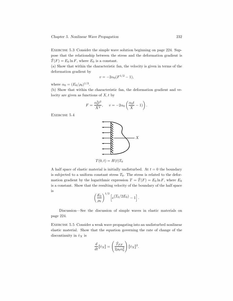
Chapter 5. Nonlinear Wave Propagation 232
Exercise 5.3 Consider the simple wave solution beginning on page 224. Sup-pose that the relationship between the stress and the deformation gradient isT (F ) = E0 lnF , where E0 is a constant.(a) Show that within the characteristic fan, the velocity is given in terms of thedeformation gradient by
v = −2α0(F 1/2 − 1),
where α0 = (E0/ρ0)1/2.(b) Show that within the characteristic fan, the deformation gradient and ve-locity are given as functions of X, t by
F =α2
0t2
X2, v = −2α0
(α0t
X− 1)
).
Exercise 5.4
X
T (0, t) = H(t)T0
�������
A half space of elastic material is initially undisturbed. At t = 0 the boundaryis subjected to a uniform constant stress T0. The stress is related to the defor-mation gradient by the logarithmic expression T = T (F ) = E0 lnF , where E0
is a constant. Show that the resulting velocity of the boundary of the half spaceis (
E0
ρ0
)1/2 [e(T0/2E0) − 1
].
Discussion—See the discussion of simple waves in elastic materials onpage 224.
Exercise 5.5 Consider a weak wave propagating into an undisturbed nonlinearelastic material. Show that the equation governing the rate of change of thediscontinuity in vX is
d
dt[[vX]] =
(TFF
2ρ0α20
)[[vX ]]2.

Chapter 5. Nonlinear Wave Propagation 233
5.3 Singular Surface Theory
A singular surface is a surface across which a field (a function of position andtime) is discontinuous. In this section we show how the theory of singularsurfaces can be used to analyze the propagation of waves in materials. Forparticular classes of waves called shock and acceleration waves, we derive thevelocity and the rate of change, or growth and decay of the amplitude for anonlinear elastic material.
Kinematic compatibility condition
Consider a scalar field φ(x, t). Suppose that at time t, the field is discontinuousat a point xs (Fig. 5.14). We denote the regions to the left and right of xs by +
x
φ(x, t)
xs
+ −
Figure 5.14: A discontinuous field.
and − , and define φ+ and φ− to be the limits of φ(x, t) as x approaches xs
from the + and − sides:
φ+ = lim(x → xs)+
φ(x, t), φ− = lim(x→ xs)−
φ(x, t).
The jump of φ(x, t) is defined by
[[φ]] = φ+ − φ−.
Now let us assume that during some interval of time the field φ(x, t) isdiscontinuous at a moving point xs given by a function
xs = xs(t).
The velocity of the point xs along the x axis is
vs =dxs(t)dt
.

Chapter 5. Nonlinear Wave Propagation 234
x
φ(x, t)
vs dt
+ − + −
�
Figure 5.15: The field φ(x, t) at time t and at time t + dt.
During the interval of time from t to t+ dt, the point xs moves a distance vs dt
(Fig. 5.15). We can express the value of φ+ at time t+ dt in terms of its valueat time t:
φ+(t + dt) = φ+(t) +(∂φ
∂t
)+
(t) dt+(∂φ
∂x
)+
(t) vs dt.
From this expression we see that the rate of change of φ+ can be expressed interms of the limits of the derivatives of φ+ at xs:
d
dtφ+ =
(∂φ
∂t
)+
+(∂φ
∂x
)+
vs. (5.39)
We can derive a corresponding expression for the rate of change of φ−:
d
dtφ− =
(∂φ
∂t
)−
+(∂φ
∂x
)−vs. (5.40)
Subtracting this equation from Eq. (5.39), we obtain an equation for the rateof change of the jump of φ(x, t):
d
dt[[φ]] =
[[∂φ
∂t
]]+
[[∂φ
∂x
]]vs. (5.41)
This equation is called the kinematic compatibility condition. When the field φ(x, t)is continuous at xs during an interval of time, [[φ]] = 0 and the kinematic com-patibility condition states that[[
∂φ
∂t
]]+
[[∂φ
∂x
]]vs = 0 (when φ is continuous). (5.42)

Chapter 5. Nonlinear Wave Propagation 235
Acceleration waves
The one-dimensional motion of a nonlinear elastic material is governed by theequation of balance of linear momentum,
ρ0∂v
∂t= TF
∂F
∂X. (5.43)
The deformation gradient and the velocity are related by
∂F
∂t=
∂v
∂X. (5.44)
An acceleration wave is a propagating singular surface across which the veloc-ity v and strain F of a material are continuous but the first partial derivatives ofthe velocity and strain are discontinuous. Thus an acceleration wave is identicalto the weak wave we discuss on page 226. Here we use the kinematic compat-ibility condition (5.41) to determine the velocity and the rate of change of theamplitude of an acceleration wave in an elastic material.
Velocity
Because v and F are continuous across an acceleration wave, by substitutingthem into Eq. (5.41) we obtain the relations[[
∂v
∂t
]]+
[[∂v
∂X
]]vs = 0 (5.45)
and [[∂F
∂t
]]+
[[∂F
∂X
]]vs = 0. (5.46)
From Eq. (5.44) we see that [[∂F
∂t
]]=
[[∂v
∂X
]]. (5.47)
The jump of the equation of balance of linear momentum, Eq. (5.43), is
ρ0
[[∂v
∂t
]]= TF
[[∂F
∂X
]].
Using Eqs. (5.45)-(5.47) we can write this equation in the form(v2
s − TF
ρ0
)[[∂v
∂t
]]= 0.
Thus the velocity of an acceleration wave in an elastic material is
vs =
(TF
ρ0
)1/2
. (5.48)
This result is identical to Eq. (5.34).

Chapter 5. Nonlinear Wave Propagation 236
Rate of change of the amplitude
We can use the jump in the acceleration of the material as a measure of theamplitude of an acceleration wave. Substituting the acceleration ∂v/∂t and∂F/∂t into Eq. (5.41), we obtain the relations
d
dt
[[∂v
∂t
]]=
[[∂2v
∂t2
]]+
[[∂2v
∂t∂X
]]vs
=[[∂2v
∂t2
]]+
[[∂2F
∂t2
]]vs
(5.49)
andd
dt
[[∂F
∂t
]]=
[[∂2F
∂t2
]]+
[[∂2F
∂t∂X
]]vs. (5.50)
From Eqs. (5.45) and (5.47),[[∂F
∂t
]]= − 1
vs
[[∂v
∂t
]].
The time derivative of this equation is
d
dt
[[∂F
∂t
]]= − 1
vs
d
dt
[[∂v
∂t
]]+
1v2
s
[[∂v
∂t
]]dvs
dt.
With this expression and Eq. (5.50), we obtain the relation[[∂2F
∂t2
]]= − 1
vs
d
dt
[[∂v
∂t
]]+
1v2
s
[[∂v
∂t
]]dvs
dt−
[[∂2F
∂t∂X
]]vs.
We substitute this result into Eq. (5.49), obtaining the expression
2d
dt
[[∂v
∂t
]]=
[[∂2v
∂t2
]]−
[[∂2F
∂t∂X
]]v2
s +1vs
[[∂v
∂t
]]dvs
dt. (5.51)
We next take the partial derivative of Eq. (5.43) with respect to time:
ρ0∂2v
∂t2= TF
∂2F
∂t∂X+ TFF
∂F
∂t
∂F
∂X,
where TFF = ∂2T /∂F 2. Taking the jump of this equation, we obtain the result[[∂2v
∂t2
]]−
[[∂2F
∂t∂X
]]v2
s =TFF
ρ0
[[∂F
∂t
∂F
∂X
]].
Using this result, we can write Eq. (5.51) in the form
2d
dt
[[∂v
∂t
]]− 1vs
[[∂v
∂t
]]dvs
dt=TFF
ρ0
[[∂F
∂t
∂F
∂X
]]. (5.52)

Chapter 5. Nonlinear Wave Propagation 237
Consider an acceleration wave that propagates into undisturbed material.In this case the velocity vs is constant and[[
∂F
∂t
∂F
∂X
]]=
[[∂F
∂t
]] [[∂F
∂X
]].
From Eqs. (5.45)-(5.47),[[∂F
∂t
]][[∂F
∂X
]]= − 1
v3s
[[∂v
∂t
]]2
.
Thus Eq. (5.52) isd
dt
[[∂v
∂t
]]= − TFF
2ρ0v3s
[[∂v
∂t
]]2
. (5.53)
This equation governs the amplitude of an acceleration wave propagating intoan undisturbed elastic material. It is identical to Eq. (5.37).
Shock waves
A shock wave in an elastic material can be modeled as a propagating singularsurface across which the motion x(X, t) of the material is continuous but thevelocity v and strain F are discontinuous. Shock waves occur commonly insupersonic gas flows, and can also occur in solid materials subjected to strongdisturbances.
Suppose that Xs is the position of a shock wave, and let us draw a free-bodydiagram of the material between positions XL and XR to the left and rightof Xs (Fig. 5.16). The equation of balance of linear momentum for the material
X
XL XS XR
TL TR+ −
�������
�������
Figure 5.16: Free-body diagram of the material between positions XL and XR.
is
TR − TL =d
dt
∫ Xs
XL
ρ0v dX +d
dt
∫ XR
Xs
ρ0v dX.

Chapter 5. Nonlinear Wave Propagation 238
Recalling that the point Xs moves with velocity vs, we can write this expressionas
TR − TL = ρ0v+vs +∫ Xs
XL
ρ0∂v
∂tdX − ρ0v−vs +
∫ XR
Xs
ρ0∂v
∂tdX.
From the limit of this equation as XS → Xs and XR → Xs we obtain the result
[[T ]] + ρ0[[v]]vs = 0. (5.54)
This equation relates the jump in the stress to the jump in the velocity acrossa shock wave. Using it together with the kinematic compatibility condition,Eq. (5.41), we can determine the velocity and the rate of change of the amplitudeof a shock wave in a nonlinear elastic material.
Velocity
Because the motion x(X, t) is continuous across a shock wave, by substitutingit into Eq. (5.41) we obtain the relation
[[v]] + [[F ]]vs = 0. (5.55)
From this relation and Eq. (5.54), we find that the velocity of a shock wave isgiven by
vs =(
[[T ]]ρ0[[F ]]
)1/2
. (5.56)
This result is independent of the stress-strain relation of the material.
Rate of change of the amplitude
Substituting the velocity and the deformation gradient into Eq. (5.41), we obtainthe relations
d
dt[[v]] =
[[∂v
∂t
]]+
[[∂v
∂X
]]vs
=[[∂v
∂t
]]+
[[∂F
∂t
]]vs
(5.57)
andd
dt[[F ]] =
[[∂F
∂t
]]+
[[∂F
∂X
]]vs. (5.58)
The jump of the equation of balance of linear momentum, Eq. (5.43), is
ρ0
[[∂v
∂t
]]=
[[∂T
∂X
]].

Chapter 5. Nonlinear Wave Propagation 239
We substitute this relation into Eq. (5.57) to obtain
d
dt[[v]] =
1ρ0
[[∂T
∂X
]]+
[[∂F
∂t
]]vs. (5.59)
Taking the time derivative of Eq. (5.55), we write the result in the form
d
dt[[v]] = −vs
d
dt[[F ]]− [[F ]]
dvs
dt.
We set this expression equal to Eq. (5.59) to obtain[[∂F
∂t
]]= − d
dt[[F ]]− 1
vs[[F ]]
dvs
dt− 1ρ0vs
[[∂T
∂X
]],
and we substitute this result into Eq. (5.58), which yields the equation
2vsd
dt[[F ]] + [[F ]]
dvs
dt=
[[∂F
∂X
]]v2
s − 1ρ0
[[∂T
∂X
]]. (5.60)
Consider a shock wave that propagates into undisturbed material. In thiscase [[
∂T
∂X
]]=
(∂T
∂X
)+
=
(dT
dF
)+
(∂F
∂X
)+
=(TF
)+
[[∂F
∂X
]],
and by taking the time derivative of Eq. (5.56), we find that
[[F ]]dvs
dt=
[1ρ0
(TF )+ − v2s
]2vs
d
dt[[F ]].
Therefore we can write Eq. (5.60) in the form
d
dt[[F ]] =
−[(TF )+ − ρ0v2s ]
[[∂F
∂X
]]
2ρ0vs
[1 +
(TF )+ − ρ0v2s
4ρ0v2s
] . (5.61)
This equation governs the rate of change of the jump in the deformation gradientof a shock wave propagating into an undisturbed elastic material. It determineswhether the amplitude of the wave grows or decays given the value of the defor-mation gradient (or the density) and the value of the gradient of the deformationgradient (or the gradient of the density) behind the wave.

Chapter 5. Nonlinear Wave Propagation 240
Exercises
Exercise 5.6 (a) Determine the relation T = T (F ) for a linear elastic material.(b) What is the velocity of an acceleration wave in a linear elastic material?(c) What is the velocity of a shock wave in a linear elastic material?
Answer: (a) T = (λ + 2μ)(F − 1). (b) α =√
(λ + 2μ)/ρ0. (c) α =√(λ+ 2μ)/ρ0.
Exercise 5.7 The relation between the stress and the deformation gradient ina material is T = T (F ) = E0 lnF , where E0 is a constant. The density of theundeformed material is ρ0.(a) What is the velocity of an acceleration wave in the undeformed material?(b) If the material is homogeneously compressed so that its density is 2ρ0, whatis the velocity of an acceleration wave?
Answer: (a) vs = (E0/ρ0)1/2. (b) vs = (2E0/ρ0)1/2.
Exercise 5.8 The relation between the stress and the deformation gradientin a material is T = T (F ) = E0 lnF , where E0 is a constant. The densityof the undeformed material is ρ0. An acceleration wave propagates into theundeformed material. At t = 0, the acceleration of the material just behindthe wave is a0 in the direction of propagation. What is the acceleration of thematerial just behind the wave at time t?
Answer:1
1a0
−(ρ0
4E0
)1/2
t
Exercise 5.9 If a gas behaves isentropically, the relation between the pressureand the density is
p
ργ=p0
ργ0
,
where γ, the ratio of specific heats, is a positive constant. In the one-dimensionalproblems we are discussing, the stress T = −p.(a) Show that the velocity of an acceleration wave propagating into undisturbedgas with pressure p0 and density ρ0 is
vs =(γp0
ρ0
)1/2
.
(b) If the amplitude [[∂v/∂t]] of an acceleration wave propagating into undis-turbed gas with pressure p0 and density ρ0 is positive, show that the amplitudeincreases with time.
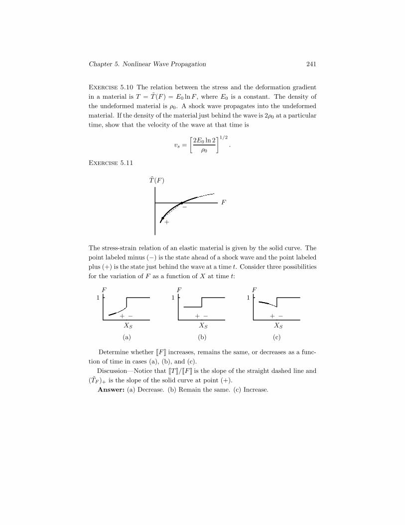
Chapter 5. Nonlinear Wave Propagation 241
Exercise 5.10 The relation between the stress and the deformation gradientin a material is T = T (F ) = E0 lnF , where E0 is a constant. The density ofthe undeformed material is ρ0. A shock wave propagates into the undeformedmaterial. If the density of the material just behind the wave is 2ρ0 at a particulartime, show that the velocity of the wave at that time is
vs =[2E0 ln 2ρ0
]1/2
.
Exercise 5.11
F
T (F )
+
−��
................................................
........
The stress-strain relation of an elastic material is given by the solid curve. Thepoint labeled minus (−) is the state ahead of a shock wave and the point labeledplus (+) is the state just behind the wave at a time t. Consider three possibilitiesfor the variation of F as a function of X at time t:
(a)
F
XS
1
+ −
(b)
F
XS
1
+ −
(c)
F
XS
1
+ −
Determine whether [[F ]] increases, remains the same, or decreases as a func-tion of time in cases (a), (b), and (c).
Discussion—Notice that [[T ]]/[[F ]] is the slope of the straight dashed line and(TF )+ is the slope of the solid curve at point (+).
Answer: (a) Decrease. (b) Remain the same. (c) Increase.
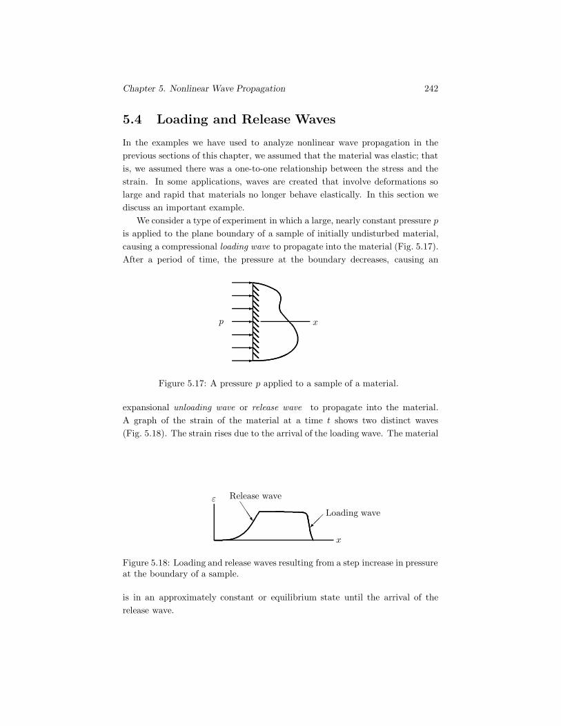
Chapter 5. Nonlinear Wave Propagation 242
5.4 Loading and Release Waves
In the examples we have used to analyze nonlinear wave propagation in theprevious sections of this chapter, we assumed that the material was elastic; thatis, we assumed there was a one-to-one relationship between the stress and thestrain. In some applications, waves are created that involve deformations solarge and rapid that materials no longer behave elastically. In this section wediscuss an important example.
We consider a type of experiment in which a large, nearly constant pressure pis applied to the plane boundary of a sample of initially undisturbed material,causing a compressional loading wave to propagate into the material (Fig. 5.17).After a period of time, the pressure at the boundary decreases, causing an
xp
�������
Figure 5.17: A pressure p applied to a sample of a material.
expansional unloading wave or release wave to propagate into the material.A graph of the strain of the material at a time t shows two distinct waves(Fig. 5.18). The strain rises due to the arrival of the loading wave. The material
x
ε Release wave
Loading wave���- ���
Figure 5.18: Loading and release waves resulting from a step increase in pressureat the boundary of a sample.
is in an approximately constant or equilibrium state until the arrival of therelease wave.

Chapter 5. Nonlinear Wave Propagation 243
Loading wave
Experiments have shown that after an initial transient period, the loading wavepropagates with nearly constant velocity and its “shape,” or waveform, is ap-proximately constant. It is then referred to as a steady wave. During this period,we can express the dependent variables in terms of a single independent variable
ζ = x− Ut,
where U is the velocity of the steady wave.The equation of conservation of mass of the material, Eq. (5.16), is
∂ρ
∂t+∂(ρv)∂x
= 0. (5.62)
By using the chain rule, we can express this equation in terms of ζ as
d
dζ[ρ(v − U)] = 0.
We see that in the steady wave, conservation of mass requires that
ρ(v − U) = constant. (5.63)
The equation of balance of linear momentum, Eq. (5.13), is
ρ
(∂v
∂t+∂v
∂xv
)= −∂p
∂x. (5.64)
In terms of ζ, it is
ρ(v − U)dv
dζ= −dp
dζ.
Using Eq. (5.63), we can write this equation in the form
d
dζ[ρ(v − U)v + p] = 0.
Thus in the steady wave, balance of linear momentum requires that
ρ(v − U)v + p = constant. (5.65)
Suppose that the steady loading wave propagates into undisturbed materialwith density ρ0 and pressure p = 0. From Eqs. (5.63) and (5.65), we obtain therelations
ρ(v − U) = −ρ0U (5.66)
andρ(v − U)v + p = 0. (5.67)
Chapter 5. Nonlinear Wave Propagation 244
Using Eq. (5.66), we can write Eq. (5.67) in the form
ρ0Uv = p. (5.68)
The strain ε of the material is related to its density by Eq. (5.15):
ε = 1 − ρ0
ρ.
By using this relation to eliminate the density from Eq. (5.66), we obtain a verysimple relation between the strain, the wave velocity, and the velocity of thematerial in the steady wave:
ε =v
U. (5.69)
With this relation we can express Eq. (5.68) in the form
p = ρ0U2ε. (5.70)
After the passage of the steady loading wave, we assume the material is in ahomogeneous, equilibrium state until the arrival of the release wave. Let ve bethe velocity of the material in the equilibrium state. Experiments have shownthat for many (but not all) materials, the velocity ve is related to the wavevelocity U by a linear relation
U = c+ sve, (5.71)
where c and s are material constants. The equilibrium state of the materialat the end of the passage of the steady wave must also satisfy Eqs. (5.69) and(5.70):
εe =ve
U,
pe = ρ0U2εe.
(5.72)
Using these two relations and Eq. (5.71), we find that
pe =ρ0c
2εe
(1 − sεe)2. (5.73)
Once the constants c and s have been determined from experiments fora particular material, the pressure pe in the equilibrium state following thepassage of the steady loading wave can be plotted as a function of the strain εe
in the equilibrium state by using Eq. (5.73). The resulting graph is called aHugoniot curve (Fig. 5.19). The pressure pe approaches infinity at the finitestrain εe = 1/s. This is an artifact of the empirical Eq. (5.71). Each pointon the Hugoniot curve for a material defines an equilibrium state following the

Chapter 5. Nonlinear Wave Propagation 245
ε
p
1s
Rayleigh lineHugoniotcurve
��.������
�
......
......
......
......
......
......
......
......
......
......
......
......
......
......
......
......
......
......
......
......
......
......
......
......
......
......
......
......
......
......
���������
Figure 5.19: The Hugoniot curve and a Rayleigh line.
passage of a steady loading wave. If any one of the four variables U , ve, pe, εe ismeasured following the passage of the wave, the other three can be determinedfrom the Hugoniot curve and Eqs. (5.72).
From Eq. (5.70), we see that the pressure is linearly related to the strainduring the passage of the steady loading wave. The resulting straight line iscalled a Rayleigh line (Fig. 5.19). The intersection of the Rayleigh line with theHugoniot curve is the equilibrium state following the passage of the wave.
Release wave
In some materials, experiments have shown that the pressure of the material andthe strain approximately follow the Hugoniot curve during the passage of therelease wave. That is, the loading of the material occurs along the Rayleigh lineand the unloading occurs (approximately) along the Hugoniot curve (Fig. 5.20).
During the passage of the release wave, the state of the material changesrelatively slowly in comparison to the rapid change of state in the loading wave.As a result, the unloading process approximately follows the Hugoniot curve,which represents equilibrium states of the material. That is, during the passageof the release wave the material can be modeled approximately as an elasticmaterial whose stress-strain relation is given by Eq. (5.73). By doing so, we canmodel the unloading wave as a simple wave. (The analysis of simple waves isdiscussed beginning on page 224.) This means that in the unloading wave thedependent variables are constant along right-running characteristics in the x-t

Chapter 5. Nonlinear Wave Propagation 246
ε
p
1s
Loadingpath Unloading
path��.
������
���
����
)������
��
��
��
��
��
�
......
......
......
......
......
......
......
......
......
......
......
......
......
......
......
......
......
......
......
......
......
......
......
......
......
......
......
......
......
......
���������
Figure 5.20: The loading and unloading paths.
plane.We can express the equations of conservation of mass, Eq. (5.62), and balance
of linear momentum, Eq. (5.64), in matrix form as
[1 00 ρ
] [ρv
]t
+
⎡⎣ v ρdp
dρρv
⎤⎦[
ρv
]x
= 0.
From Eq. (5.21), the slope c of a right-running characteristic is given by
c = v +(dp
dρ
)1/2
= v +[(1 − ε)2
ρ0
dp
dε
]1/2
.
This expression relates the slopes of the characteristics defining the motion of therelease wave to the slope of the Hugoniot curve. We can arrive at two conclusionsfrom this relation and Fig. 5.20. First, since the slope of the Hugoniot decreasesas the strain decreases, the high-strain (leading) part of the release wave travelsfaster than the low-strain (trailing) part. As a result, the release wave “spreads”with increasing time. Second, because the slope of the Hugoniot curve at highstrain is larger than the slope of the Rayleigh line, we see from the secondof Eqs. (5.72) that the high-strain part of the release wave travels faster thanthe loading wave. Eventually (if the sample is large enough) the release waveovertakes the loading wave. As a result, the amplitude of the loading wave isattenuated.
The integral of the pressure with respect to the strain as the loading andunloading waves pass through the material is the cross-hatched area between
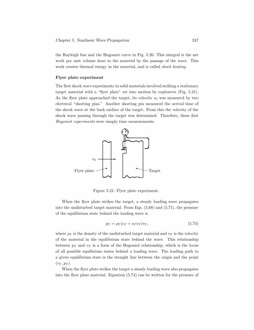
Chapter 5. Nonlinear Wave Propagation 247
the Rayleigh line and the Hugoniot curve in Fig. 5.20. This integral is the network per unit volume done to the material by the passage of the wave. Thiswork creates thermal energy in the material, and is called shock heating.
Flyer plate experiment
The first shock wave experiments in solid materials involved striking a stationarytarget material with a “flyer plate” set into motion by explosives (Fig. 5.21).As the flyer plate approached the target, its velocity v0 was measured by twoelectrical “shorting pins.” Another shorting pin measured the arrival time ofthe shock wave at the back surface of the target. From this the velocity of theshock wave passing through the target was determined. Therefore, these firstHugoniot experiments were simply time measurements.
v0
Flyer plate Target
�
���* ����
�........................� ........................ �
����
Figure 5.21: Flyer plate experiment.
When the flyer plate strikes the target, a steady loading wave propagatesinto the undisturbed target material. From Eqs. (5.68) and (5.71), the pressureof the equilibrium state behind the loading wave is
pT = ρT (cT + sT vT )vT , (5.74)
where ρT is the density of the undisturbed target material and vT is the velocityof the material in the equilibrium state behind the wave. This relationshipbetween pT and vT is a form of the Hugoniot relationship, which is the locusof all possible equilbrium states behind a loading wave. The loading path toa given equilibrium state is the straight line between the origin and the point(vT , pT ).
When the flyer plate strikes the target a steady loading wave also propagatesinto the flyer plate material. Equation (5.74) can be written for the pressure of

Chapter 5. Nonlinear Wave Propagation 248
the equilibrium state behind the loading wave in the flyer plate,
pF = ρF (cF + sF vF )vF , (5.75)
where vF is the velocity of the material in the equilibrium state toward the left,relative to the undisturbed flyer plate. Relative to a stationary reference frame,the velocity of the flyer-plate material in the equilibrium state toward the rightis v0 − vF , where v0 is the initial velocity of the flyer plate. Because the flyerplate and target are in contact,
pT = pF (5.76)
andvT = v0 − vF . (5.77)
vT
p
00 v0
pT pF
Loading pathHugoniot
Loading pathHugoniot��.
���.
�������
�
..........................................................................................................................................................................................................................................
............
............
............
............
............
..................
............
............
............
............
..................
............
............
............
............
.........
Figure 5.22: Hugoniot curves for a flyer plate experiment.
Figure 5.22 shows the locus of equilibrium states for the target material givenby Eq. (5.74). Using Eqs. (5.75) and (5.77), we also show the locus of equilib-rium states for the flyer plate material as a function of vT . The point wherethese curves intersect determines the velocity and pressure of the materials inthe equilibrium regions behind the steady loading waves. The dashed straightlines are the Rayleigh lines, the loading paths followed by the two materials inchanging from their undisturbed states to the equilibrium state.

Chapter 5. Nonlinear Wave Propagation 249
A Little History
As we have mentioned, large-amplitude steady loading waves are also calledshock waves, and the pivotal relationship to the development of the field ofshock physics was Eq. 5.70:
p = ρ0U2(1 − ρ0/ρ).
This relationship was derived in 1859 by the Reverend S. Earnshaw. Unfor-tunately, he assumed that all steady waves must be elastic phenomena. Heconcluded that steady waves could only exist in materials with a one-to-onerelationship between stress and strain given by this expression. As he believedthat air obeyed Boyle’s Law,
p = p0ρ/ρ0 ,
he concluded that, because these two expressions do not agree, shock wavescould not exist in air. As anyone who has heard a supersonic aircraft passknows, Earnshaw’s conclusion was wrong. Indeed shock waves will propagatein nearly all materials, because they induce behaviors that are not elastic. Aswe have observed, shock waves induce heating in materials.
The study of thermal phenomena was undergoing fundamental change dur-ing Earnshaw’s day. The old caloric theory of heat was being abandoned andreplaced by the modern laws of thermodynamics. We now understand that en-ergy is conserved while being converted in part from a mechanical form to heat.And in fact, shock waves cause entropy to increase. In contrast, as the releasewave passes, the material response is isentropic. While we have approximatedthe release path by the Hugoniot, the path is actually an isentrope (path ofconstant entropy) that falls slightly above the Hugoniot and accounts for theeffects of thermal expansion in the material (Fig. 5.23).
It would be another decade before Rankine analyzed the shock wave andconcluded that ”there must be both a change of temperature and a conductionof heat” in order that steady waves might exist. And it was not until the late1880’s that Hugoniot eliminated the need for heat conduction from the theoryof shock waves. See Drumheller (1998).

Chapter 5. Nonlinear Wave Propagation 250
ε
p
1s
Rayleigh lineHugoniotcurve
Isentrope
Thermalexpansion
︸︷︷︸
�����.
��.������
�
......
......
......
......
......
......
......
......
......
......
......
......
......
......
......
......
......
......
......
......
......
......
......
......
......
......
......
......
......
......
���������
Figure 5.23: The isentrope and resulting thermal expansion.

Chapter 5. Nonlinear Wave Propagation 251
Exercises
Exercise 5.12 Consider a flyer plate experiment in which the flyer plate andthe target are identical materials with mass density 2.79 Mg/m3, the measuredshock wave velocity is 6.66 km/s, and the measured flyer-plate velocity is 2 km/s.What is the pressure in the equilibrium region behind the loading wave?
Answer: 18.6 GPa.
Exercise 5.13 (a) Suppose that in the experiment of Exercise 5.12, the flyerplate is aluminum with properties ρ0 = 2.79 Mg/m2, c = 5.33 km/s, ands = 1.40, the target is stainless steel with properties ρ0 = 7.90 Mg/m2, c =4.57 km/s, and s = 1.49, and the velocity of the flyer plate is 2 km/s. Whatis the pressure in both materials in the equilibrium region behind the loadingwave, and what is the velocity of their interface?(b) If the materials are interchanged so that the flyer plate is stainless steel andthe target is aluminum, what is the pressure in both materials in the equilibriumregion behind the loading wave and what is the velocity of their interface?
Answer: (a) Pressure is 27 GPa, velocity is 630 m/s.
Exercise 5.14 In Exercise 5.13, assume that the target is much thicker thanthe flyer plate. After the loading wave in the flyer plate reaches the back surfaceof the flyer plate, it is reflected as a release wave and returns to the interfacebetween the materials. Determine whether the plates separate when the releasewave reaches the interface: (a) if the flyer plate is aluminum and the target isstainless steel; (b) if the flyer plate is stainless steel and the target is aluminum.
Answer: (a) Yes. (b) No.

Bibliography
Achenbach, J. D., Wave Propagation in Elastic Solids, North-Holland Publish-ing Company, Amsterdam, 1987.
Becker, E. B., Carey, G. F, and Oden, J. T., Finite Elements, An Introduction,Volume 1, Prentice-Hall, Inc., Englewood Cliffs, New Jersey, 1981.
Brekhovskikh, L. M., Waves in Layered Media, Academic Press, New York,1980.
Brillouin, L., Wave Propagation and Group Velocity, Academic Press, New York,1960.
Brillouin, L., Wave Propagation in Periodic Structures, Dover Publications,Inc., New York, 1953.
Courant, R., and Friedrichs, K. O., Supersonic Flow and Shock Waves, Springer-Verlag, Heidelberg, 1985.
Chen, P. J., Selected Topics in Wave Propagation, Noordhoff International Pub-lishing, Leyden, 1976.
Drumheller, D. S., Introduction to Wave Propagation in Nonlinear Fluids andSolids, Cambridge University Press, 1998.
Ewing, W. M., Elastic Waves in Layered Media, Ulan Press, 2012.
Fung, Y. C., Foundations of Solid Mechanics, Prentice-Hall, Inc., EnglewoodCliffs, New Jersey, 1965.
252

Chapter 5. Nonlinear Wave Propagation 253
Gould, P. L., Introduction to Linear Elasticity, Springer-Verlag, New York, 1983.
Graff, K. F., Wave Motion in Elastic Solids, Dover Publications Inc., Mineola,New York, 1991.
Hamming, R. W., Digital Filters, Prentice-Hall, Inc., New Jersey, 1983.
Hughes, T. J. R., The Finite Element Method, Linear Static and Dynamic FiniteElement Analysis, Dover Publications, Inc., Mineola, New York, 2000.
Jeffrey, A., and Taniuti, T., Non-Linear Wave Propagation with Applications toPhysics and Magnetohydrodynamics, Academic Press, New York, 1964.
Kolsky, H., Stress Waves in Solids, Dover Publications, Inc., Mineola New York,2012.
Lighthill, J., Waves in Fluids, Cambridge University Press, 1980.
Miklowitz, J., The Theory of Elastic Waves and Waveguides, North-HollandPublishing Company, Amsterdam, 1978.
Press, W. H., Flannery, B. P., Teukolsky, S. A., and Vetterling, W. T., NumericalRecipes, Cambridge University Press, 1986.
Royer, D., Dieulesaint, E., and Morgan, D. P., Elastic Waves in Solids I: Freeand Guided Propagation, Springer, New York, 2000.
van der Hijden, J. H. M. T., Propagation of Transient Elastic Waves in StratifiedAnisotropic Media, Elsevier Scientific Publishing Co., Amsterdam, 1987.
Wasley, R. J., Stress Wave Propagation in Solids, Marcel Dekker, Inc., NewYork, 1973.
Whitham, G. B., Linear and Nonlinear Waves, John Wiley and Sons, New York,1974.
Zel’dovich, Y. B., and Raizer, Y. P., Physics of Shock Waves and High-TemperatureHydrodynamic Phenomena, Vols. I and II, Academic Press, New York, 1966.

Index
acceleration, 9in linear elasticity, 11material description, 9spatial description, 11
acceleration wave, 235amplitude, 236velocity, 235
acoustic impedance, 72acoustic medium, 44acoustic waves in a channel, 143
cutoff frequencies of, 147modes of, 146phase velocities of, 146
alternator, 3amplitude, 111
complex, 113anisotropic material, 32
balance of angular momentum, 40balance of linear momentum, 39, 42
in linear elasticity, 43in terms of potentials, 44
band-limited function, 173basis functions, 81body forces, 28boundary conditions
displacement, 54for a string, 61free, 57stress, 55
bulk modulus, 45
Cagniard-de Hoop method, 196cartesian coordinates, 1characteristics, 94, 219
initial-boundary value problem,95
initial-value problem, 94circular frequency, 113compressional (P ) wave, 55
reflection of, 126speed of, 55
conservation of mass, 21, 38in linear elasticity, 21
convective acceleration, 11cross product, 3curl, 4cutoff frequency, 147cycles, 113
D’Alembert solution, 50, 63, 111deformation gradient, 214del operator, 5discrete Fourier transform, 172
examples, 174inversion, 173
dispersion, 107, 147, 182dispersion relation, 149
for a layer, 149for layered media, 156
displacement, 9, 213displacement boundary condition, 54displacement equations of motion,
254
Chapter 5. Nonlinear Wave Propagation 255
42, 46divergence, 4dot product, 3
elastic material, 32displacement equations of mo-
tion of, 42, 46isotropic, 32linear, 32nonlinear, 216stress-strain relations for, 34
elasticitylinear, 1nonlinear, 213
elements, 79Eulerian (spatial) description, 10
FFT (fast Fourier transform), 174finite element method, 78Floquet theorem, 156flyer plate experiment, 247Fourier superposition, 167Fourier transform, 164
definition, 164discrete, 172example, 164FFT, 174inversion, 164
free boundary, 57, 73frequency, 112, 113
circular, 113frequency components, 172frequency spectrum, 172
Gauss theorem, 4gradient, 4group velocity, 183
half space, 54Helmholtz decomposition, 43, 46
Hertz, 113Hugoniot curve, 244hyperbolic equations, 220
impulse response, 167incident wave, 70index notation, 1indices, 1initial-boundary value problems, 66interior equation, 220inverse motion, 9isotropic material, 32
stress-strain relations for, 34
Jordan’s lemma, 163
kinematic compatibility condition, 234Kronecker delta, 3
Lagrangian (material) description, 10Lagrangian strain tensor, 15Lame constants, 34, 46Lamb’s problem, 196Laplace transform, 159
definition, 159example, 160inversion, 159
layered media, 99steady-state waves in, 154transient waves in, 106unit cell of, 154
linear elasticity, 11acceleration in, 11displacement equations of mo-
tion, 42displacement equations of mo-
tion in, 46strain tensor in, 15velocity in, 11
linear strain tensor, 15

Chapter 5. Nonlinear Wave Propagation 256
loading wave, 242, 243longitudinal strain, 15
mass matrix, 85material description, 10material volume, 37method of characteristics, 93, 220modes, 146modulus of elasticity, 36motion, 9
inverse, 9
nodes, 81normal stress, 25Nyquist frequency, 173
one-dimensional wave equationD’Alembert solution of, 50for a string, 61
one-dimensional waves, 48initial-boundary value problems,
66reflection and transmission of,
70wave speed of, 50
pass band, 157period, 112phase velocity
of a one-dimensional wave, 111phase wave, 183plane strain, 118plane waves, 119
displacement field of, 121wavelength of, 120
plate velocity, 151Poisson’s ratio, 34, 36Poisson’s ratio, 34propagation, 52propagation direction, 120
propagation modes, 146
Rayleigh line, 245Rayleigh wave, 140
particle trajectories, 143phase velocity, 141
Rayleigh-Lamb modes, 149reference state, 8reflected wave, 70, 114
from a free boundary, 73from a material interface, 70from a rigid boundary, 73
reflection and transmission, 70release wave, 242, 245resonance, 114rigid boundary, 73
sampling theorem, 173scalar field, 4scalar potential, 43, 46shear (S) wave, 58
critical angle of, 134reflection of, 132
shear modulus, 34shear strain, 17, 18shear stress, 25shear waves, 57shock heating, 247shock wave, 231, 237
amplitude, 239history, 249velocity, 238
simple waves, 224singular surface, 233slowness, 198spatial description, 10steady wave, 243steady-state waves, 110
amplitude of, 111

Chapter 5. Nonlinear Wave Propagation 257
complex amplitude of, 113complex form of, 113frequency of, 112in a layer, 147in layered media, 154modes, 146one-dimensional, 110period of, 112phase velocity of, 111plane, 119propagation direction of, 120resonance of, 114two-dimensional, 118wave number of, 111wavelength of, 111
stiffness matrix, 85stop band, 157strain
in nonlinear elasticity, 214longitudinal, 15shear, 17, 18
strain tensor, 15in linear elasticity, 15, 47
stress boundary condition, 55stress tensor, 26stress-strain relation
in linear elasticity, 32in nonlinear elasticity, 32, 216
stress-strain relations, 34, 47string
boundary conditions for, 61equation of motion of, 60lateral motion of, 60
summation convention, 2surface wave, 141
tetrahedron argument, 26traction, 24, 29, 47transient waves, 110, 159
in layered media, 185transmitted wave, 70, 114transport theorem, 37, 38
undulating bore, 107unloading (release) wave, 242, 245
variational formulation, 84vector field, 4vector Laplacian, 43vector potential, 43, 46velocity, 9
in linear elasticity, 11in nonlinear elasticity, 213material description of, 9spatial description of, 11
wave equation, 44D’Alembert solution of, 50, 63one-dimensional, 48
wave number, 111wave speed
of a compressional wave, 55of a one-dimensional wave, 52of a shear wave, 58
wavelength, 111weak (variational) formulation, 84weak wave
growth and decay, 231velocity, 227, 229
weak waves, 227
Young’s modulus, 34, 36

Solutions to the Exercises
Chapter 1. Linear Elasticity
Exercise 1.1 Show that δkmukvm = ukvk.
Solution—In terms of the numerical values of the indices, the left side ofthe equation is
δkmukvm = δ11u1v1 + δ12u1v2 + δ13u1v3+δ21u2v1 + δ22u2v2 + δ23u2v3+δ31u3v1 + δ32u3v2 + δ33u3v3
= (1)u1v1 + (0)u1v2 + (0)u1v3+(0)u2v1 + (1)u2v2 + (0)u2v3+(0)u3v1 + (0)u3v2 + (1)u3v3
= u1v1 + u2v2 + u3v3.
The right side of the equation is
ukvk = u1v1 + u2v2 + u3v3.
Exercise 1.2
(a) Show that δkmekmn = 0.(b) Show that δkmδkn = δmn .
Solution—(a)
δkmekmn = δ11e11n + δ12e12n + δ13e13n
+δ21e21n + δ22e22n + δ23e23n
+δ31e31n + δ32e32n + δ33e33n
= e11n + e22n + e33n.
258
Solutions, Chapter 1. Linear Elasticity 259
Because ekmn = 0 if any two of its indices are equal, e11n = 0, e22n = 0, ande33n = 0 for any value of n.
(b) Let m = 1 and n = 1.
δk1δk1 = δ11δ11 + δ21δ21 + δ31δ31
= δ11.
The procedure is the same for each value of m and n.
Exercise 1.3 Show that Tkmδmn = Tkn.
Solution—Let k = 1 and n = 1.
T1mδm1 = T11δ11 + T12δ21 + T13δ31
= T11.
The procedure is the same for each value of k and n.
Exercise 1.4 If Tkmekmn = 0, show that Tkm = Tmk.
Solution—Let n = 1 and recall that ekmn = 0 if any two of the subscriptsk, m, and n are equal. Thus
Tkmekm1 = T23e231 + T32e321 = T23 − T32 = 0,
so T32 = T23. By letting n = 2 and then n = 3, the same procedure shows thatT13 = T31 and T12 = T21.
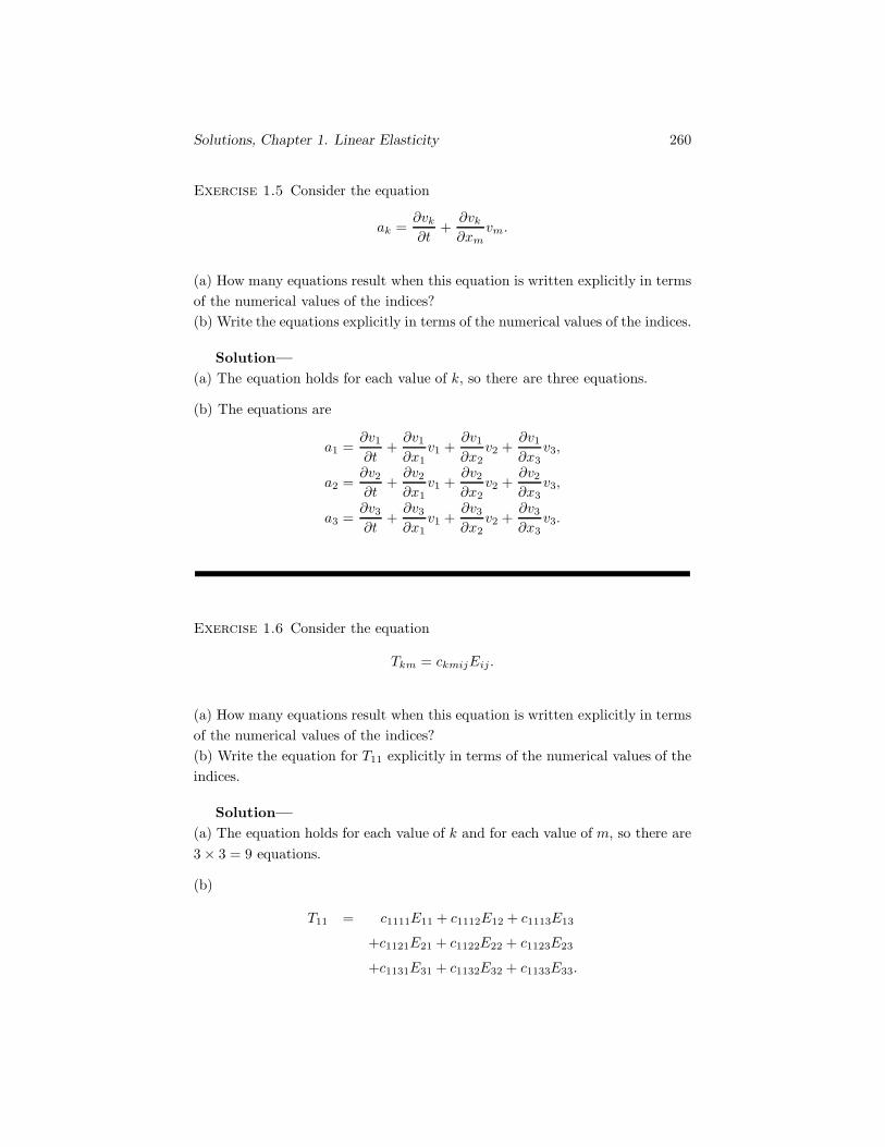
Solutions, Chapter 1. Linear Elasticity 260
Exercise 1.5 Consider the equation
ak =∂vk
∂t+∂vk
∂xmvm.
(a) How many equations result when this equation is written explicitly in termsof the numerical values of the indices?(b) Write the equations explicitly in terms of the numerical values of the indices.
Solution—(a) The equation holds for each value of k, so there are three equations.
(b) The equations are
a1 =∂v1∂t
+∂v1∂x1
v1 +∂v1∂x2
v2 +∂v1∂x3
v3,
a2 =∂v2∂t
+∂v2∂x1
v1 +∂v2∂x2
v2 +∂v2∂x3
v3,
a3 =∂v3∂t
+∂v3∂x1
v1 +∂v3∂x2
v2 +∂v3∂x3
v3.
Exercise 1.6 Consider the equation
Tkm = ckmijEij.
(a) How many equations result when this equation is written explicitly in termsof the numerical values of the indices?(b) Write the equation for T11 explicitly in terms of the numerical values of theindices.
Solution—(a) The equation holds for each value of k and for each value of m, so there are3 × 3 = 9 equations.
(b)
T11 = c1111E11 + c1112E12 + c1113E13
+c1121E21 + c1122E22 + c1123E23
+c1131E31 + c1132E32 + c1133E33.

Solutions, Chapter 1. Linear Elasticity 261
Exercise 1.7 The “del operator” is defined by
∇(·) =∂(·)∂x1
i1 +∂(·)∂x2
i2 +∂(·)∂x3
i3
=∂(·)∂xk
ik.(1.78)
The expression for the gradient of a scalar field φ in terms of cartesian coordi-nates can be obtained in a formal way by applying the del operator to the scalarfield:
∇φ =∂φ
∂xkik.
(a) By taking the dot product of the del operator with a vector field v, obtainthe expression for the divergence ∇·v in terms of cartesian coordinates. (b) Bytaking the cross product of the del operator with a vector field v, obtain theexpression for the curl ∇× v in terms of cartesian coordinates.
Solution—(a) The divergence is
∇ · v =[∂(·)∂xk
ik
]· [vm im]
=∂vm
∂xk(ik · im)
=∂vm
∂xkδkm
=∂vk
∂xk.
(b) The curl is
∇× v =[∂(·)∂xk
ik
]× [vm im]
=∂vm
∂xk(ik × im)
=∂vm
∂xkekmn in.

Solutions, Chapter 1. Linear Elasticity 262
Exercise 1.8 By expressing the dot and cross products in terms of index no-tation, show that for any two vectors u and v,
u · (u × v) = 0.
Solution—u · (u× v) = (ur ir) · (ukvmekmn in)
= urukvmekmn(ir · in)= urukvmekmnδrn
= unukvmekmn.
The term unukekmn = 0. For example, let m = 1. Then
unukek1n = u2u3e312 + u3u2e213 = u2u3 − u3u2 = 0.
Exercise 1.9 Show that
ukvmekmnin = det
⎡⎣ i1 i2 i3u1 u2 u3
v1 v2 v3
⎤⎦ .
Solution—The i1 component of the left side of the equation is
ukvmekm1 = u2v3e231 + u3v2e321 = u2v3 − u3v2.
The i1 component of the determinant is
u2v3 − u3v2.
In the same way, the i2 and i3 components can be shown to be equal.
Exercise 1.10 By expressing the divergence and curl in terms of index nota-tion, show that for any vector field v for which the indicated derivatives exist,
∇ · (∇× v) = 0.
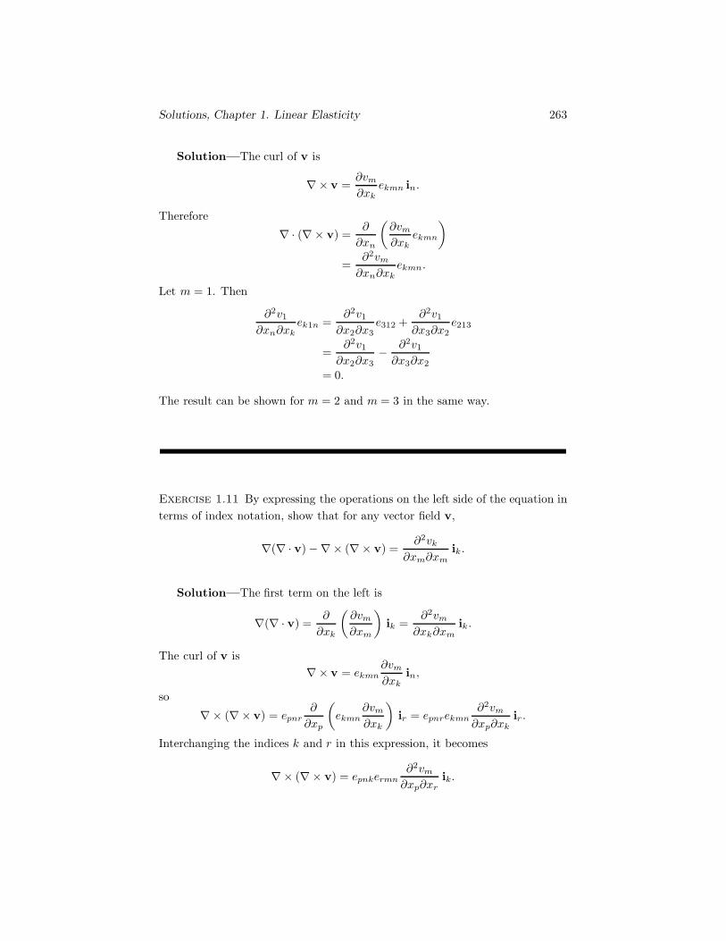
Solutions, Chapter 1. Linear Elasticity 263
Solution—The curl of v is
∇× v =∂vm
∂xkekmn in.
Therefore
∇ · (∇× v) =∂
∂xn
(∂vm
∂xkekmn
)=
∂2vm
∂xn∂xkekmn.
Let m = 1. Then
∂2v1∂xn∂xk
ek1n =∂2v1∂x2∂x3
e312 +∂2v1∂x3∂x2
e213
=∂2v1∂x2∂x3
− ∂2v1∂x3∂x2
= 0.
The result can be shown for m = 2 and m = 3 in the same way.
Exercise 1.11 By expressing the operations on the left side of the equation interms of index notation, show that for any vector field v,
∇(∇ · v) −∇× (∇× v) =∂2vk
∂xm∂xmik.
Solution—The first term on the left is
∇(∇ · v) =∂
∂xk
(∂vm
∂xm
)ik =
∂2vm
∂xk∂xmik.
The curl of v is∇× v = ekmn
∂vm
∂xkin,
so
∇× (∇× v) = epnr∂
∂xp
(ekmn
∂vm
∂xk
)ir = epnrekmn
∂2vm
∂xp∂xkir .
Interchanging the indices k and r in this expression, it becomes
∇× (∇× v) = epnkermn∂2vm
∂xp∂xrik.

Solutions, Chapter 1. Linear Elasticity 264
Therefore we must show that
∂2vm
∂xm∂xk− epnkermn
∂2vm
∂xp∂xr=
∂2vk
∂xm∂xm. (∗)
This equation must hold for each value of k. Let k = 1. The right side of theequation is
∂2v1∂xm∂xm
=∂2v1∂x1∂x1
+∂2v1∂x2∂x2
+∂2v1∂x3∂x3
.
On the left side of Eq. (∗), let us sum over the index n:
∂2vm
∂xm∂x1−epn1ermn
∂2vm
∂xp∂xr=
∂2vm
∂xm∂x1−(ep11erm1+ep21erm2+ep31erm3)
∂2vm
∂xp∂xr.
The term ep11 = 0. Also, ep21 is zero unless p = 3 and ep31 is zero unless p = 2.Therefore this expression is
∂2vm
∂xm∂x1+ erm2
∂2vm
∂x3∂xr− erm3
∂2vm
∂x2∂xr=
∂2v1∂x1∂x1
+∂2v2∂x2∂x1
+∂2v3∂x3∂x1
+∂2v1∂x3∂x3
− ∂2v3∂x3∂x1
− ∂2v2∂x2∂x1
+∂2v1∂x2∂x2
=∂2v1∂x1∂x1
+∂2v1∂x2∂x2
+∂2v1∂x3∂x3
.
Thus the left side of Eq. (∗) equals the right side for k = 1. The procedure isthe same for k = 2 and k = 3.
Exercise 1.12 Consider a smooth, closed surface S with outward-directed unitvector n. Show that ∫
S
n dS = 0.
Solution—The x1 component of the integral is∫S
n1 dS.
This integral is of the form ∫S
vknk dS,
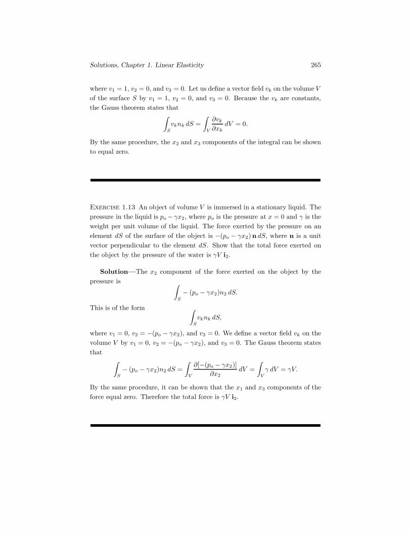
Solutions, Chapter 1. Linear Elasticity 265
where v1 = 1, v2 = 0, and v3 = 0. Let us define a vector field vk on the volume Vof the surface S by v1 = 1, v2 = 0, and v3 = 0. Because the vk are constants,the Gauss theorem states that∫
S
vknk dS =∫
V
∂vk
∂xkdV = 0.
By the same procedure, the x2 and x3 components of the integral can be shownto equal zero.
Exercise 1.13 An object of volume V is immersed in a stationary liquid. Thepressure in the liquid is po − γx2 , where po is the pressure at x = 0 and γ is theweight per unit volume of the liquid. The force exerted by the pressure on anelement dS of the surface of the object is −(po − γx2)n dS, where n is a unitvector perpendicular to the element dS. Show that the total force exerted onthe object by the pressure of the water is γV i2.
Solution—The x2 component of the force exerted on the object by thepressure is ∫
S
− (po − γx2)n2 dS.
This is of the form ∫S
vknk dS,
where v1 = 0, v2 = −(po − γx2), and v3 = 0. We define a vector field vk on thevolume V by v1 = 0, v2 = −(po − γx2), and v3 = 0. The Gauss theorem statesthat ∫
S
− (po − γx2)n2 dS =∫
V
∂[−(po − γx2)]∂x2
dV =∫
V
γ dV = γV.
By the same procedure, it can be shown that the x1 and x3 components of theforce equal zero. Therefore the total force is γV i2.

Solutions, Chapter 1. Linear Elasticity 266
Exercise 1.14 A bar of material 1 meter long is subjected to the “stretching”motion
x1 = X1(1 + t2), x2 = X2, x3 = X3.
(a) Determine the inverse motion of the bar.(b) Determine the material description of the displacement.(c) Determine the spatial description of the displacement.(d) What is the displacement of a point at the right end of the bar when t = 2seconds?
Solution—(a) Solving the motion for X1, X2, and X3 in terms of x1, x2, x3, and t, weobtain
X1 = x1/(1 + t2), X2 = x2, and X3 = x3.
(b) By using the motion, the three components of the displacement are
u1 = x1 −X1 = X1(1 + t2) −X1 = X1t2,
u2 = x2 −X2 = X2 −X2 = 0,u3 = x3 −X3 = X3 −X3 = 0.
(c) From the results of Parts (a) and (b),
u1 = X1t2 =
x1
(1 + t2)t2, u2 = 0, and u3 = 0.
(d) At the right end of the bar, X1 = 1 m. From the result of Part (b),
u1 = X1t2 = (1)(2)2 = 4 m, u2 = 0, and u3 = 0.
Exercise 1.15 Consider the motion of the bar described in Exercise 1.14.(a) Determine the material description of the velocity.(b) Determine the spatial description of the velocity.(c) Determine the material description of the acceleration.(d) Determine the spatial description of the acceleration by substituting theinverse motion into the result of Part (c).(e) Determine the spatial description of the acceleration by using Eq. (1.13).

Solutions, Chapter 1. Linear Elasticity 267
Solution—(a) From the motion,
v1 =∂x1
∂t=
∂
∂t[X1(1 + t2)] = 2X1t,
v2 =∂x2
∂t=
∂
∂t(X2) = 0,
v3 =∂x3
∂t=
∂
∂t(X3) = 0.
(b) By using the inverse motion and the expressions we obtained in Part (a),
v1 = 2X1t = 2x1t/(1 + t2), v2 = 0, and v3 = 0.
(c)
a1 =∂v1∂t
=∂
∂t[2X1t] = 2X1,
a2 =∂v2∂t
= 0,
a3 =∂v3∂t
= 0.
(d)
a1 = 2X1 =2x1
1 + t2, a2 = 0, and a3 = 0.
(e)
a1 =∂v1∂t
+∂v1∂x1
v1 +∂v1∂x2
v2 +∂v1∂x3
v3
=∂
∂t
(2x1t
1 + t2
)+
[∂
∂x1
(2x1t
1 + t2
)](2x1t
1 + t2
)
=2x1
(1 + t2)− 2x1t
(1 + t2)2(2t) +
2t(1 + t2)
2x1t
(1 + t2)
=2x1
1 + t2.
Exercise 1.16 A 1 meter cube of material is subjected to the “shearing” mo-tion
x1 = X1 +X22 t
2, x2 = X2, x3 = X3.

Solutions, Chapter 1. Linear Elasticity 268
(a) Determine the inverse motion of the cube.(b) Determine the material description of the displacement.(c) Determine the spatial description of the displacement.(d) What is the displacement of a point at the upper right edge of the cubewhen t = 2 seconds?
Solution—(a) Solving the motion for X1, X2, and X3 in terms of x1, x2, x3, and t, weobtain
X1 = x1 −X22 t
2 = x1 − x22t
2, X2 = x2, and X3 = x3.
(b) By using the motion, the three components of the displacement are
u1 = x1 −X1 = X1 +X22 t
2 −X1 = X22 t
2,u2 = x2 −X2 = X2 −X2 = 0,u3 = x3 −X3 = X3 −X3 = 0.
(c) From the results of Parts (a) and (b),
u1 = X22 t
2 = x22t
2, u2 = 0, and u3 = 0.
(d) At the upper right edge of the cube, X1 = 1 m and X2 = 1 m. From theresult of Part (b),
u1 = X22 t
2 = (1)2(2)2 = 4 m, u2 = 0, and u3 = 0.
Exercise 1.17 Consider the motion of the cube described in Exercise 1.16.(a) Determine the material description of the velocity.(b) Determine the spatial description of the velocity.(c) Determine the material description of the acceleration.(d) Determine the spatial description of the acceleration by substituting theinverse motion into the result of Part (c).(e) Determine the spatial description of the acceleration by using Eq. (1.13).
Solution—

Solutions, Chapter 1. Linear Elasticity 269
(a) From the motion,
v1 =∂x1
∂t=
∂
∂t[X1 +X2
2 t2] = 2X2
2 t,
v2 =∂x2
∂t=
∂
∂t(X2) = 0,
v3 =∂x3
∂t=
∂
∂t(X3) = 0.
(b) By using the inverse motion and the expressions we obtained in Part (a),
v1 = 2X22 t = 2x2
2t, v2 = 0, and v3 = 0.
(c)
a1 =∂v1∂t
=∂
∂t[2X2
2t] = 2X22 ,
a2 =∂v2∂t
= 0,
a3 =∂v3∂t
= 0.
(d)a1 = 2X2
2 = 2x22, a2 = 0, and a3 = 0.
(e)
a1 =∂v1∂t
+∂v1∂x1
v1 +∂v1∂x2
v2 +∂v1∂x3
v3
=∂
∂t(2x2
2t)
= 2x22.
Exercise 1.18 Show that the acceleration is given in terms of derivatives ofthe spatial description of the velocity by
ak =∂vk
∂t+∂vk
∂xnvn.
Solution—By substituting the motion into the spatial description of thevelocity field, we obtain the expression
vk = vk(xn, t) = vk(xn(Xm, t), t) = vk(Xm, t).

Solutions, Chapter 1. Linear Elasticity 270
The acceleration is the time derivative of this expression with X held fixed:
ak =∂
∂tvk(Xm, t) =
∂vk
∂t+∂vk
∂xn
∂xn
∂t.
Because∂xn
∂t= vn,
we obtain the resultak =
∂vk
∂t+∂vk
∂xnvn.
Exercise 1.19 A bar of material 1 meter long is subjected to the “stretching”motion
x1 = X1(1 + t2), x2 = X2, x3 = X3.
(a) Determine the Lagrangian strain tensor of the bar at time t.(b) Use the motion to determine the length of the bar when t = 2 seconds.(c) Use the Lagrangian strain tensor to determine the length of the bar whent = 2 seconds.
Solution—(a) The material description of the displacement field is
u1 = x1 −X1 = X1(1 + t2) −X1 = X1t2,
u2 = x2 −X2 = X2 −X2 = 0,u3 = x3 −X3 = X3 −X3 = 0.
The Lagrangian strain tensor is
Emn =12
(∂um
∂Xn+
∂un
∂Xm+
∂uk
∂Xm
∂uk
∂Xn
)The only non-zero component is
E11 =12
(∂u1
∂X1+∂u1
∂X1+∂u1
∂X1
∂u1
∂X1
)= 1
2 [t2 + t2 + (t2)(t2)]
= t2 + 12t4.
(b) From the motion we can see that at t = 2 seconds the left end of the bar islocated at
x1 = X1(1 + t2) = (0)[1 + (2)2] = 0

Solutions, Chapter 1. Linear Elasticity 271
and the right end of the bar is located at
x1 = X1(1 + t2) = (1)[1 + (2)2] = 5 meters.
Therefore the length of the bar is 5 meters.
(c) From Part (a), at t = 2 seconds
E11 = t2 + 12t
4 = (2)2 + 12(2)4 = 12.
We can determine the longitudinal strain ε of the material from the equation
2ε+ ε2 = 2Emnnmnn.
Let us determine the longitudinal strain in the x1 direction by setting n1 = 1,n2 = 0, and n3 = 0:
2ε+ ε2 = 2E11(1)(1) = 24.
The solution of this equation is ε = 4. (The root ε = −6 can be ignored sincethe longitudinal strain must be greater than -1.)
At t = 2 seconds, the length ds of an element of the bar parallel to thex1 axis is related to its length dS in the reference state by
ds− dS
dS= ε = 4.
Thereforeds = (1 + 4) dS = 5 dS,
and the length of the bar at t = 2 seconds is∫ 1
0
5 dS = 5 meters.
Exercise 1.20 An object consists of a 1 meter cube in the reference state. Attime t, the value of the linear strain tensor at each point of the object is
[Ekm] =
⎡⎣ 0.001 −0.001 0
−0.001 0.002 00 0 0
⎤⎦ .
(a) What is the length of the edge AB at time t?(b) What is the length of the diagonal AC at time t?(c) What is the angle θ at time t?

Solutions, Chapter 1. Linear Elasticity 272
Solution—(a) In linear elasticity, the longitudinal strain ε is given by ε = Emnnmnn. Todetermine the longitudinal strain in the direction of the edge AB, let n1 = 1,n2 = 0, and n3 = 0:
ε = E11(1)(1) = E11 = 0.001.
Therefore at time t the length ds of an element of the edge AB is related to itslength dS in the reference state by
ds− dS
dS= ε = 0.001,
sods = (1 + 0.001) dS
The length of the edge AB at time t is∫ 1
0
(1 + 0.001) dS = 1.001 meter.
(b) To determine the longitudinal strain in the direction of the diagonal AC,we let n1 = 1/
√2, n2 = 1/
√2, and n3 = 0:
ε = E11n1n1 +E12n1n2 + E21n2n1 +E22n2n2
= (0.001)(1/√
2)(1/√
2) + 2(−0.001)(1/√
2)(1/√
2) + (0.002)(1/√
2)(1/√
2)= 0.0005.
Therefore at time t the length ds of an element of the diagonal AC is related toits length dS in the reference state by
ds− dS
dS= ε = 0.0005,
sods = (1 + 0.0005) dS
The length of the diagonal AC at time t is
∫ √2
0
(1 + 0.001) dS = 1.0005√
2meter.
(c) At time t, the angle between line elements originally parallel to the x1 and x2
axes is given in terms of the linear strain tensor by π/2 − 2E12. Therefore theangle θ at time t is
θ = π/2 + 2E12 = (π/2 − 0.002) rad.

Solutions, Chapter 1. Linear Elasticity 273
Exercise 1.21 Show that in linear elasticity,
∂uk
∂Xm=∂uk
∂xm.
Discussion—Use the chain rule to write∂uk
∂Xm=∂uk
∂xn
∂xn
∂Xm,
and use Eq. (1.5).
Solution—The displacement is
uk = uk(xn, t) = uk(xn(Xm, t), t) = uk(Xm, t).
Therefore∂uk
∂Xm=∂uk
∂xn
∂xn
∂Xm. (∗)
From the relationxn = Xn + un
we obtain the result∂xn
∂Xm= δnm +
∂un
∂Xm.
Substituting this into Eq. (∗) gives
∂uk
∂Xm=∂uk
∂xm+∂uk
∂xn
∂un
∂Xm. (∗∗)
This equation contains the derivative ∂un/∂Xm on the right side. By changingindices, we can write the equation as
∂un
∂Xm=∂un
∂xm+∂un
∂xr
∂ur
∂Xm.
We can substitute this expression into the right side of Eq. (∗∗). Continuing inthis way, we obtain the infinite series
∂uk
∂Xm=∂uk
∂xm+∂uk
∂xn
∂un
∂xm+∂uk
∂xn
∂un
∂xr
∂ur
∂xm+ · · ·
In linear elasticity, we neglect higher order terms in the derivatives of the dis-placement and this equation reduces to
∂uk
∂Xm=∂uk
∂xm.

Solutions, Chapter 1. Linear Elasticity 274
Exercise 1.22 Consider Eq. (1.27):
2E12 = (1 + 2E11)12 (1 + 2E22)
12 cos(π/2 − γ12).
In linear elasticity, the terms E11, E22, E12, and the shear strain γ12 are small.Show that in linear elasticity this relation reduces to
γ12 = 2E12.
Solution—Let us expand the term (1 + 2E11)12 in a Taylor series in terms
of the small term E11:
(1 + 2E11)12 = [(1 + 2E11)
12 ]E11=0 +
{d
dE11[(1 + 2E11)
12 ]}
E11=0
E11 + · · ·
= 1 + E11 + · · ·
Next, we expand the term cos(π/2−γ12) in a Taylor series in terms of the smallterm γ12:
cos(π/2 − γ12) = [cos(π/2 − γ12)]γ12=0 +{
d
dγ11[cos(π/2 − γ12)]
}γ12=0
γ12 + · · ·
= γ12 + · · ·
Therefore the equation can be written
2E12 = (1 +E11 + · · ·)(1 +E22 + · · ·)(γ12 + · · ·).
If we neglect higher order terms, the equation reduces to
2E12 = γ12.
Exercise 1.23 By using Eqs. (1.30) and (1.32), show that in linear elasticitythe density ρ is related to the density ρ0 in the reference state by Eq. (1.33).
Solution—From the equations
ρ0 dV0 = ρ dV

Solutions, Chapter 1. Linear Elasticity 275
anddV = (1 + Ekk) dV0,
we see thatρ
ρ0= (1 +Ekk)−1.
We expand the expression on the right in terms of the small term Ekk:
(1 + Ekk)−1 = [(1 +Ekk)−1]Ekk=0 +{
d
dEkk[(1 + Ekk)−1]
}Ekk=0
Ekk + · · ·
= 1 − Ekk + · · ·
Therefore in linear elasticity
ρ
ρ0= 1 −Ekk.
Exercise 1.24 A stationary square bar is acted upon by uniform normal trac-tions σ0 at the ends (Fig. 1). As a result, the components of the stress tensorat each point of the material are
[Tkm] =
⎡⎣ σ0 0 0
0 0 00 0 0
⎤⎦ .
(a) Determine the magnitudes of the normal and shear stresses acting on theplane shown in Fig. 2 by writing equilibrium equations for the free body diagramshown.(b) Determine the magnitudes of the normal and shear stresses acting on theplane shown in Fig. 2 by using Eq. (1.36).
Solution—(a) The normal stress σ and shear stress τ acting on the plane are shown:
σ0
σ
τ
30◦����
$$��������
$$/$$/$$/$$/$$/$$/$$/$$/
��0��0��0

Solutions, Chapter 1. Linear Elasticity 276
If we denote the cross sectional area of the bar by ΔA, the area of the plane thestesses σ and τ act on is ΔA/ cos 30◦:
Area = ΔA Area = ΔA/ cos 30◦
30◦����
���.
����
......
......
......
......
......
......
......
......
......
......
The sum of the forces in the direction normal to the plane must equal zero:
σ(ΔA/ cos 30◦) − (σ0ΔA) cos 30◦ = 0.
Therefore |σ| = σ0 cos2 30◦.The sum of the forces in the direction parallel to the plane must equal zero:
τ (ΔA/ cos30◦) + (σ0ΔA) sin 30◦ = 0.
From this equation we see that |τ | = σ0 sin 30◦ cos 30◦.
(b) In terms of the coordinate system shown, the components of the unit vector nnormal to the plane are n1 = cos 30◦, n2 = sin 30◦, and n3 = 0. Therefore thecomponents of the traction vector acting on the plane are
t1 = T1mnm = T11n1 + T12n2 + T13n3 = σ0 cos 30◦,t2 = T2mnm = T21n1 + T22n2 + T23n3 = 0,t3 = T3mnm = T31n1 + T32n2 + T33n3 = 0.
The normal stress acting on the plane is
σ = t · n = t1n1 + t2n2 + t3n3 = σ0 cos2 30◦.
The shear stress is the component of the vector t parallel to the plane. Itsmagnitude is
|t1 sin 30◦ − t2 cos 30◦| = σ0 sin 30◦ cos 30◦.
Exercise 1.25 The components of the stress tensor at each point of the cubeof material shown in Fig. 1 are
[Tkm] =
⎡⎣ T11 T12 0T12 T22 00 0 T33
⎤⎦ .

Solutions, Chapter 1. Linear Elasticity 277
Determine the magnitudes of the normal and shear stresses acting on the planeshown in Fig. 2.
Solution—The components of the unit vector normal to the plane are n1 =cos θ, n2 = sin θ, and n3 = 0. The components of the traction vector acting onthe plane are
t1 = T1mnm = T11n1 + T12n2 + T13n3 = T11 cos θ + T12 sin θ,t2 = T2mnm = T21n1 + T22n2 + T23n3 = T12 cos θ + T22 sin θ,t3 = T3mnm = T31n1 + T32n2 + T33n3 = 0.
The normal stress acting on the plane is
σ = t · n = t1n1 + t2n2 + t3n3
= (T11 cos θ + T12 sin θ)(cos θ) + (T12 cos θ+ T22 sin θ)(sin θ)= T11 cos2 θ+ 2T12 sin θ cos θ + T22 sin2 θ.
The shear stress is the component of the vector t parallel to the plane. Itsmagnitude is
|t1 sin θ − t2 cos θ| = |T12(cos2 θ− sin2 θ) − (T11 − T22) sin θ cos θ|.
Exercise 1.26 The components of the stress tensor at each point of the cubeof material shown in Fig. 1 are
[Tkm] =
⎡⎣ 100 −100 0
−100 100 00 0 300
⎤⎦ Pa.
A pascal (Pa) is 1 newton/meter2 . Determine the magnitudes of the normaland shear stresses acting on the plane shown in Fig. 2.
Solution—The unit vector perpendicular to the plane is
n =1√3(i1 + i2 + i3).
The traction vector acting on the plane is
{tk} = [Tkm]{nm} =
⎡⎣ 100 −100 0
−100 100 00 0 300
⎤⎦⎡⎣ 1/
√3
1/√
31/
√3
⎤⎦
=
⎡⎣ 0
0100
√3
⎤⎦ Pa.

Solutions, Chapter 1. Linear Elasticity 278
The normal stress is
σ = t1n1 + t2n2 + t3n3 = (100√
3)(1/√
3) = 100 Pa.
The component of t parallel to the surface is the shear stress:
{tk − σnk} =
⎡⎣ 0
0100
√3
⎤⎦− 100
⎡⎣ 1/
√3
1/√
31/
√3
⎤⎦ =
100√3
⎡⎣ −1
−12
⎤⎦ .
The magnitude of this vector is τ = 100√
2 Pa.
Exercise 1.27 The Lame constants of an isotropic material are λ = 1.15(1011) Paand μ = 0.77(1011) Pa. The components of the strain tensor at a point P inthe material are
[Ekm] =
⎡⎣ 0.001 −0.001 0
−0.001 0.001 00 0 0.002
⎤⎦ .
Determine the components of the stress tensor Tkm at point P .
Solution—From the stress-strain relation, Eq. (1.43), the stress componentT11 is
T11 = λδ11(E11 +E22 + E33) + 2μE11 = (λ+ 2μ)E11 + λ(E22 + E33)
= [1.15(1011) + 2(0.77)(1011)](0.001)
+1.15(1011)(0.001 + 0.002)
= 6.14(108) Pa.
The stress component T12 is
T12 = λδ12(E11 + E22 +E33) + 2μE12 = 2μE12
= 2(0.77)(1011)(−0.001)
= −1.54(108) Pa.
Continuing in this way, the stress tensor is
[Tkm] =
⎡⎣ 6.14(108) −1.54(108) 0
−1.54(108) 6.14(108) 00 0 7.68(108)
⎤⎦ Pa.

Solutions, Chapter 1. Linear Elasticity 279
Exercise 1.28 A bar is 200 mm long and has a square 50 mm × 50 mm crosssection in the unloaded state. The bar consists of isotropic material with Lameconstants λ = 4.5(1010) Pa and μ = 3.0(1010) Pa. The ends of the bar aresubjected to a uniform normal traction σ0 = 2.0(108) Pa. As a result, thecomponents of the stress tensor at each point of the material are
[Tkm] =
⎡⎣ 2.0(108) 0 0
0 0 00 0 0
⎤⎦ Pa.
(a) Determine the length of the bar in the loaded state.(b) Determine the dimensions of the square cross section of the bar in the loadedstate.
Solution—Because the stress components are known, the stress-strain re-lation, Eq. (1.43), can be solved for the components of the strain. The resultsare
[Ekm] =
⎡⎣ 2.564(10−3) 0 0
0 −7.692(10−4) 00 0 −7.692(10−4)
⎤⎦ .
The length of the loaded bar is
(200mm)(1 +E11) = (200mm)[1 + 2.564(10−3)] = 200.513 mm.
The height and width of the loaded bar are
(50mm)(1 +E22) = (50mm)[1 − 7.692(10−4)] = 4.9962 mm,
so the dimensions of the cross section are 4.9962 mm × 4.9962 mm.
Exercise 1.29 The ends of a bar of isotropic material are subjected to a uni-form normal traction T11. As a result, the components of the stress tensor ateach point of the material are
[Tkm] =
⎡⎣ T11 0 0
0 0 00 0 0
⎤⎦ .

Solutions, Chapter 1. Linear Elasticity 280
(a) The ratio E of the stress T11 to the longitudinal strainE11 in the x1 direction,
E =T11
E11,
is called the Young’s modulus, or modulus of elasticity of the material. Showthat the Young’s modulus is related to the Lame constants by
E =μ(3λ + 2μ)λ+ μ
(b) The ratio
ν = −E22
E11
is called the Poisson’s ratio of the material. Show that the Poisson’s ratio isrelated to the Lame constants by
ν =λ
2(λ + μ)
Solution—From the stress-strain relation, Eq. (1.43),
T11 = λ(E11 +E22 + E33) + 2λE11 = (λ+ 2μ)E11 + 2λE22, (∗)
where we have used the fact that E22 = E33, and
T22 = 0 = λ(E11 +E22 + E33) + 2λE22 = λE11 + 2(λ + μ)E22.
From the latter equation,
E22 =−λ
2(λ + μ)E11. (∗∗)
Substituting this relation into Eq. (*) yields
T11 = (λ+ 2μ)E11 −2λ2
2(λ + μ)E11,
So Young’s modulus is
E =T11
E11= λ+ 2μ− λ2
λ + μ=μ(3λ + 2μ)λ+ μ
,
and from Eq. (**), Poisson’s ratio is
ν = −E22
E11=
λ
2(λ+ μ).

Solutions, Chapter 1. Linear Elasticity 281
Exercise 1.30 The Young’s modulus and Poisson’s ratio of an elastic materialare defined in Exercise 1.29. Show that the Lame constants of an isotropicmaterial are given in terms of the Young’s modulus and Poisson’s ratio of thematerial by
λ =νE
(1 + ν)(1 − 2ν), μ =
E
2(1 + ν).
Solution—The relations derived in Exercise 1.29 are
E =μ(3λ + 2μ)λ+ μ
, (∗)
ν =λ
2(λ + μ). (∗∗)
Solving Eq. (**) for μ,
μ =(1 − 2ν)
2νλ. (∗ ∗ ∗)
Substituting this expression into Eq. (*) and simplifying yields
E =(1 + ν)(1− 2ν)
νλ,
soλ =
νE
(1 + ν)(1− 2ν).
Then substituting this result into Eq. (***) gives the result
μ =E
2(1 + ν).
Exercise 1.31 Show that the strain components of an isotropic linear elasticmaterial are given in terms of the stress components by
Ekm =12μTkm − λ
2μ(3λ + 2μ)δkmTjj.
Solution—The stress-strain relation is
Tkm = λδkmEjj + 2μEkm. (∗)

Solutions, Chapter 1. Linear Elasticity 282
Setting m = k,Tkk = 3λEjj + 2μEkk = (3λ+ 2μ)Ekk,
and solving for Ekk,
Ekk =1
3λ + 2μTkk. (∗∗)
Solving Eq. (*) for Ekm,
Ekm =12μTkm − λ
2μδkmEjj.
and substituting the expression (**) for Ejj yields
Ekm =12μTkm − λ
2μ(3λ + 2μ)δkmTjj.
Exercise 1.32 By using the Gauss theorem, Eq. (1.3), the transport theorem,Eq. (1.45), and the equation of conservation of mass, Eq. (1.46), show thatEq. (1.48),
d
dt
∫V
ρvm dV =∫
S
Tmknk dS +∫
V
bm dV,
can be expressed in the form∫V
(ρam − ∂Tmk
∂xk− bm
)dV = 0,
where am is the acceleration of the material.
Solution—Applying the transport theorem to the term on the left,
d
dt
∫V
ρvm dV =∫
V
[∂
∂t(ρvm) +
∂
∂xr(ρvmvr)
]dV
=∫
V
{vm
[∂ρ
∂t+∂(ρvr)∂xr
]︸ ︷︷ ︸
= 0
+ρ[∂vm
∂t+∂vm
∂xrvr
]︸ ︷︷ ︸
= am
}dV
=∫
V
ρam dV.
Applying the Gauss theorem to the first term on the right,∫S
Tmknk dS =∫
V
∂Tmk
∂xkdV.
Substituting these two expressions into the equation gives the desired equation.

Solutions, Chapter 1. Linear Elasticity 283
Exercise 1.33 Show that the postulate of balance of angular momentum fora material
d
dt
∫V
x× ρv dV =∫
S
x× t dS +∫
V
x× b dV
implies that the stress tensor is symmetric:
Tkm = Tmk.
Solution—In terms of indices, the postulate is
d
dt
∫V
ekmnxkρvm dV =∫
S
ekmnxktm dS +∫
V
ekmnxkbm dV. (∗)
Using the transport theorem, the left side of this equation is
d
dt
∫V
ekmnxkρvm dV =∫
V
[∂
∂t(ekmnxkρvm) +
∂
∂xr(ekmnxkρvmvr)
]dV
=∫
V
[ekmnxk
(∂ρ
∂tvm + ρ
∂vm
∂t
)+ ekmnδkrρvmvr
+ekmnxk∂(ρvr)∂xr
vm + ekmnxkρvr∂vm
∂xr
]dV
=∫
V
{ekmnxkvm
[∂ρ
∂t+∂(ρvr)∂xr
]+ ekmnxkρ
[∂vm
∂t+∂vm
∂xrvr
]}dV
=∫
V
ekmnxkρam dV,
where we have observed that ekmnδkrρvmvr = ekmnρvmvk = 0.The first term on the right side of Eq. (∗) is∫
S
ekmnxktm dS =∫
S
ekmnxkTmrnr dS
=∫
V
ekmn∂
∂xr(xkTmr) dV
=∫
V
(ekmnδkrTmr + ekmnxk
∂Tmr
∂xr
)dV.
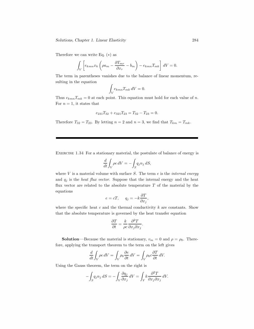
Solutions, Chapter 1. Linear Elasticity 284
Therefore we can write Eq. (∗) as∫V
[ekmnxk
(ρam − ∂Tmr
∂xr− bm
)− ekmnTmk
]dV = 0.
The term in parentheses vanishes due to the balance of linear momentum, re-sulting in the equation ∫
V
ekmnTmk dV = 0.
Thus ekmnTmk = 0 at each point. This equation must hold for each value of n.For n = 1, it states that
e231T32 + e321T23 = T32 − T23 = 0.
Therefore T32 = T23. By letting n = 2 and n = 3, we find that Tkm = Tmk.
Exercise 1.34 For a stationary material, the postulate of balance of energy is
d
dt
∫V
ρe dV = −∫
S
qjnj dS,
where V is a material volume with surface S. The term e is the internal energyand qj is the heat flux vector. Suppose that the internal energy and the heatflux vector are related to the absolute temperature T of the material by theequations
e = cT, qj = −k ∂T∂xj
,
where the specific heat c and the thermal conductivity k are constants. Showthat the absolute temperature is governed by the heat transfer equation
∂T
∂t=
k
ρc
∂2T
∂xj∂xj.
Solution—Because the material is stationary, vm = 0 and ρ = ρ0. There-fore, applying the transport theorem to the term on the left gives
d
dt
∫V
ρe dV =∫
V
ρ0∂e
∂tdV =
∫V
ρ0c∂T
∂tdV.
Using the Gauss theorem, the term on the right is
−∫
S
qjnj dS = −∫
V
∂qj
∂xjdV =
∫V
k∂2T
∂xj∂xjdV.

Solutions, Chapter 1. Linear Elasticity 285
The balance of energy postulate becomes∫V
[ρ0c
∂T
∂t− k
∂2T
∂xj∂xj
]dV,
which yields the heat transfer equation.
Exercise 1.35 By substituting the Helmholtz decomposition u = ∇φ+∇×ψinto the equation of balance of linear momentum (1.56), show that the equationof balance of linear momentum can be written in the form
∇[ρ0∂2φ
∂t2− (λ + 2μ)∇2φ
]+ ∇×
[ρ0∂2ψ
∂t2− μ∇2ψ
]= 0.
Solution—Substituting the Helmholtz decomposition into Eq. (1.56), itbecomes
ρ0∂2
∂t2(∇φ+ ∇×ψ) = (λ+ 2μ)∇(∇2φ) − μ∇× [∇× (∇× ψ)],
where we have used the identies ∇· (∇×ψ) = 0 and ∇×∇φ = 0. This equationcan be written
∇[ρ0∂2φ
∂t2− (λ+ 2μ)∇2φ
]+ ∇×
[ρ0∂2ψ
∂t2+ μ∇× (∇× ψ)
]= 0. (∗)
Taking the curl of the definition
∇2ψ = ∇(∇ · ψ) −∇× (∇× ψ)
gives∇×∇2ψ = 0 −∇× [∇× (∇×ψ)].
Using this expression in Eq. (*) gives the desired result.

Solutions, Chapter 2. One-Dimensional Waves 286
Exercise 1.36 An acoustic medium is defined in Section 1.7. Show that thedensity ρ of an acoustic medium is governed by the wave equation
∂2ρ
∂t2= α2∇2ρ.
Solution—The motion of an acoustic medium is governed by the equation
∂2u∂t2
= α2∇(∇ · u),
or in terms of indices,
∂2uk
∂t2= α2 ∂2um
∂xm∂xk= α2∂Emm
∂xk.
Let us take the divergence of this vector equation by taking the derivative withrespect to xk:
∂2Ekk
∂t2= α2 ∂2Ekk
∂xm∂xm. (∗)
Notice that we interchanged the indices on the right side of the equation.The density ρ is given in terms of the strain by
ρ = ρ0(1 −Ekk).
From this equation we see that
∂2ρ
∂t2= −ρ0
∂2Ekk
∂t2,
∂2ρ
∂xm∂xm= −ρ0
∂2Ekk
∂xm∂xm.
With these results we can write Eq. (*) in the form
∂2ρ
∂t2= α2 ∂2ρ
∂xm∂xm,
or∂2ρ
∂t2= α2∇2ρ.
Chapter 2. One-Dimensional Waves
Exercise 2.1 A function f(x) is defined by
x < 0 f(x) = 0,
0 ≤ x ≤ 1 f(x) = sin(πx),
x > 1 f(x) = 0.

Solutions, Chapter 2. One-Dimensional Waves 287
Plot the function f(ξ) = f(x − αt) as a function of x for t = 0, t = 1 s, andt = 2 s if α = 1.
Solution—
x
f(x − αt)t = 0
−1 0 1 2 3 40
1
x
f(x − αt)t = 1 s
−1 0 1 2 3 40
1
x
f(x − αt)t = 2 s
−1 0 1 2 3 40
1
Exercise 2.2 Show that as time increases, the graph of the function g(η) =g(x+αt) as a function of x translates in the negative x direction with constantvelocity α.
Solution—Modify the argument used on page 50 to show that the graphof f(ξ) translates in the positive x direction with constant velocity α.
Exercise 2.3 By using the chain rule, show that the second partial derivativeof u = u(x, t) with respect to x can be expressed in terms of partial derivativesof u = u(ξ, η) by
∂2u
∂x2=∂2u
∂ξ2+ 2
∂2u
∂ξ∂η+∂2u
∂η2.

Solutions, Chapter 2. One-Dimensional Waves 288
Solution—The dependent variable u is
u = u(x, t) = u(ξ, η),
where ξ = x−αt and η = x+αt. Applying the chain rule, the partial derivativeof u with respect to x is
∂u
∂x=
∂ξ
∂x
∂u
∂ξ+∂η
∂x
∂u
∂η
=∂u
∂ξ+∂u
∂η.
Then by applying the chain rule again,
∂2u
∂x2=
∂
∂x
(∂u
∂ξ+∂u
∂η
)
=∂ξ
∂x
∂
∂ξ
(∂u
∂ξ+∂u
∂η
)
+∂η
∂x
∂
∂η
(∂u
∂ξ+∂u
∂η
)
=(∂2u
∂ξ2+ 2
∂2u
∂ξ∂η+∂2u
∂η2
).
Exercise 2.4 Show that the D’Alembert solution
u = f(ξ) + g(η)
is a solution of the one-dimensional wave equation
∂2u
∂t2= α2∂
2u
∂x2.
Solution—Because the equation is linear, it is sufficient to show that f(ξ)and g(η) are each solutions. The partial derivative of f(ξ) with respect to t is
∂f
∂t=∂ξ
∂t
df
dξ= −αdf
dξ.

Solutions, Chapter 2. One-Dimensional Waves 289
Then by applying the chain rule again,
∂2f
∂t2=
∂
∂t
(−αdf
dξ
)=∂ξ
∂t
d
dξ
(−αdf
dξ
)= α2d
2f
dξ2.
It can be shown in the same way that
∂2f
∂x2=d2f
dξ2.
Thus f(ξ) is a solution of the one-dimensional wave equation. The same proce-dure can be used to show that g(η) is a solution.
Exercise 2.5 Consider the expression
u = Aei(kx − ωt).
What conditions must the constants A, k, and ω satisfy in order for this expres-sion to be a solution of the one-dimensional wave equation, Eq. (2.1)?
Solution—Substituting the expression into the one-dimensional wave equa-tion, the result can be written
A(ω2 − α2k2)ei(kx − ωt) = 0.
Except for the trivial solutions A = 0 and ω = k = 0, the expression is a solutiononly if the constants ω and k satisfy the relation ω2/k2 = α2. In that case, noconstraint is placed on the constant A.
Exercise 2.6 Consider the first-order partial differential equation
∂u
∂t+ α
∂u
∂x= 0,
where α is a constant. By expressing it in terms of the independent variablesξ = x− αt and η = x+ αt, show that its general solution is
u = f(ξ),

Solutions, Chapter 2. One-Dimensional Waves 290
where f is an arbitrary twice-differentiable function.
Solution—Let u = u(x, t) = u(ξ, η). Then
∂u
∂t=∂ξ
∂t
∂u
∂ξ+∂η
∂t
∂u
∂η= −α∂u
∂ξ+ α
∂u
∂η
and
∂u
∂x=∂ξ
∂x
∂u
∂ξ+∂η
∂x
∂u
∂η=∂u
∂ξ+∂u
∂η.
Substituting these expressions into the first-order equation yields the equation
∂u
∂η= 0.
Integrating yields the general solution
u = f(ξ).
Exercise 2.7 A particular type of steel has Lame constants λ = 1.15×10¹¹ Paand μ = 0.77 × 10¹¹ Pa and density ρ0 = 7800 kg/m3. Determine (a) thecompressional wave velocity α; (b) the shear wave velocity β.
Solution—(a):
α =
√λ+ 2μρ0
=
√(1.15× 10¹¹) + 2(0.77× 10¹¹)
7800= 5870 m/s.
(b):
β =√μ
ρ0=
√0.77× 10¹¹
7800= 3140 m/s.
Exercise 2.8 Consider the steel described in Exercise 2.7. A compressionalwave propagates through the material. The displacement field is
u1 = 0.001 sin[2(x1 − αt)] m, u2 = 0, u3 = 0.

Solutions, Chapter 2. One-Dimensional Waves 291
Determine the maximum normal stress T11 caused by the wave.
Solution—From the stress-strain relation
Tkm = λδkmEjj + 2μEkm,
The stress component T11 is
T11 = λ(E11 +E22 + E33) + 2μE11.
For the given displacement field, E22 and E33 are zero and
E11 =∂u1
∂x1= (0.001)(2) cos[2(x1 − αt)].
The maximum value of E11 is 0.002, so the maximum value of T11 is
T11 = (λ + 2μ)E11 = [1.15× 10¹¹ + 2(0.77× 10¹¹](0.002) = 538 MPa,
where MPa denotes a megapascal, or 106 pascals.
Exercise 2.9 Suppose that at t = 0 the velocity of an unbounded elastic ma-terial is zero and its displacement field is described by u1(x1, 0) = p(x1), where
x1 < 0 p(x1) = 0,
0 ≤ x1 ≤ 1 p(x1) = A sin(πx1),
x1 > 1 p(x1) = 0,
where A is a constant. Plot the displacement field as a function of x1 whent = 0, t = 1/(2α), and t = 1/α.
Solution—The displacement field at time t is given by Eq. (2.19):

Solutions, Chapter 2. One-Dimensional Waves 292
x1
u1
t = 0
−2 −1 0 1 2 30
A
x1
u1
t = 1/2α
−2 −1 0 1 2 30
A
x1
u1
t = 1/α
−2 −1 0 1 2 30
A
Exercise 2.10 Suppose that a half space of elastic material is initially undis-turbed and at t = 0 the boundary is subjected to a uniform normal stressT11 = T H(t), where T is a constant and the Heaviside, or step function H(t)is defined by
H(t) ={
0 when t < 0,1 when t ≥ 0.
(a) Show that the resulting displacement field in the material is
u1 = − αT
λ+ 2μ
(t − x1
α
)H
(t− x1
α
).
(b) Assume that T/(λ+2μ) = 1. Plot the displacement field as a function of x1
when αt = 1, αt = 2, and αt = 3.
Solution—(a) The solution to this type of problem is discussed in the sec-tion beginning on page 66. The displacement field is given by Eq. (2.26), where
p(t) =1
λ + 2μT11(0, t).
In this exercise, p(t) = [T/(λ+ 2μ)]H(t), so
u1 = − αT
λ + 2μ
∫ t−x1/α
0
H(t) dt = − αT
λ+ 2μ
(t− x1
α
)H
(t − x1
α
).

Solutions, Chapter 2. One-Dimensional Waves 293
(b)
x1
u1
t = 1/αt = 2/αt = 3/α
0 1 2 3 4−4
−3
−2
−1
0
1
$$$$$$
$$$$$$$$$$$$
$$$$$$$$$$$$$$$$$$
��
��
���&
��
��
��&
��
���&
Exercise 2.11 Consider a plate of elastic material of thickness L. Assume thatthe plate is infinite in extent in the x2 and x3 directions. Suppose that the plateis initially undisturbed and at t = 0 the left boundary is subjected to a uniformnormal stress T11 = T H(t), where T is a constant and the step function H(t)is defined in Exercise 2.10. This boundary condition will give rise to a wavepropagating in the positive x1 direction. When t = L/α, the wave will reachthe right boundary and cause a reflected wave. Show that from t = L/α untilt = 2L/α the displacement field in the plate is
u1 = − αT
λ+ 2μ
[(t − x1
α
)H
(t− x1
α
)+
(t+
x1
α− 2L
α
)H
(t+
x1
α− 2L
α
)].
Solution—The solution for the wave propagating in the positive x1 direc-tion is discussed in the section beginning on page 66. The displacement field isgiven by Eq. (2.26):
u1(x1, t) = f(ξ) = −α∫ t−x1
α
0
p(t) dt, (∗) (2.79)
wherep(t) =
1λ + 2μ
T11(0, t).
Setting T11(0, t) = T H(t), we obtain the displacement field
u1 = − αT
λ + 2μ
(t− x1
α
)H
(t− x1
α
).

Solutions, Chapter 2. One-Dimensional Waves 294
After the wave reaches the boundary at x1 = L there will be a reflected wavepropagating in the negative x1 direction. Assume a displacement field
u1(x1, t) = f(ξ) + g(η). (∗∗)
The boundary condition at x1 = L is T11(L, t) = 0, which means that
∂u1
∂x1(L, t) = 0.
Evaluating the partial derivative,
∂u1
∂x1=df(ξ)dξ
∂ξ
∂x1+dg(η)dη
∂η
∂x1
= − 1α
df(ξ)dξ
+1α
dg(η)dη
.
The boundary condition is
− 1α
df(t − L
α)
d(t− L
α)
+1α
dg(t+L
α)
d(t+L
α)
= 0.
Defining t = t+ L/α, this is
dg(t)dt
=df(t − 2L
α)
d(t− 2Lα
)
Integrating this equation yields
g(t) = f(t − 2Lα
) + C,
where C is a constant. Using this expression and Eqs. (*) and (*) gives thesolution.
Exercise 2.12 Confirm that the solution (2.18) satisfies the initial conditions (2.12).
Solution—It’s obvious that the displacement initial condition is satisfied,u1(x1, 0) = p(x1). To confirm that the velocity initial condition is satisfied, we

Solutions, Chapter 2. One-Dimensional Waves 295
use the following result from calculus: if the limits of an integral are functionsof a parameter y,
I =∫ b(y)
a(y)
f(x) dx,
the derivative of the integral with respect to y is
dI
dy= f(b(y))
db(y)dy
− f(a(y))da(y)dy
.
The solution (2.18) is
u(x1, t) =12p(ξ) +
12p(η) +
12α
∫ η
ξ
q(x) dx,
so∂u1
∂t=
12dp(ξ)dξ
∂ξ
∂t+
12dp(η)dη
∂η
∂t+
12α
[q(η)
∂η
∂t− q(ξ)
∂ξ
∂t
]= −α
2dp(ξ)dξ
+α
2dp(η)dη
+12[q(η) + q(ξ)]
Setting t = 0 in this expression yields
∂u1
∂t(x1, 0) = q(x1).
Exercise 2.13 Confirm that the solution (2.26) satisfies the boundary condi-tion (2.24).
Solution—The solution (2.26) is
u1(x1, t) = −α∫ ξ
0
p(t) dt.
Using the result from calculus quoted in the previous solution,
∂u1
∂x1= −αp(ξ) ∂ξ
∂x1= p(ξ).
Setting x1 = 0 in this expression yields
∂u1
∂x1(0, t) = p(t).

Solutions, Chapter 2. One-Dimensional Waves 296
Exercise 2.14 By using Eqs. (2.80) and (2.81), show that the quantity v+αwis constant along any straight line in the x-t plane having slope
dx
dt= −α.
Solution—The change in the quantity v + αw from the point x, t to thepoint x+ dx, t+ dt is
d(v + αw) =∂
∂t(v + αw) dt+
∂
∂x(v + αw) dx
=(∂v
∂t+ α
∂w
∂t
)dt+
(∂v
∂x+ α
∂w
∂x
)dx.
By using Eqs. (2.80) and (2.81), we can write this expression in the form
d(v + αw) =(∂v
∂x+
1α
∂v
∂t
)(dx+ α dt) .
Thus d(v + αw) is zero ifdx
dt= −α.
Exercise 2.15 Suppose that a half space of elastic material is initially undis-turbed, and at t = 0 the boundary is subjected to the stress boundary condition
T11(0, t) = p(t),
where p(t) is a prescribed function of time that vanishes for t < 0. Use themethod of characteristics to determine the velocity and strain of the materialat an arbitrary point x1, t in the x1-t plane.
Answer:v(x1, t) = − α
λ + 2μp(t− x1
α
),
w(x1, t) =1
λ + 2μp(t − x1
α
).
Solution—The boundary condition is
T11(0, t) = (λ+ 2μ)∂u1
∂x1(0, t) = (λ + 2μ)w(0, t) = p(t),

Solutions, Chapter 2. One-Dimensional Waves 297
orw(0, t) =
1λ+ 2μ
p(t).
We want to determine the solution at a point x1, t in the x1-t plane. Extend-ing left-running and right-running characteristics from this point, we obtain thefollowing diagram:
x1
t
t− x1/α
x1, t
b
c
a
d��
�
������
����������������
The initial condition states that v and w equal zero on the x1 axis. From thecharacteristic ad, we obtain the equation
ad : v(x1, t) + αw(x1, t) = 0.
From ab, we obtain
ab : v(x1, t) − αw(x1, t) = v(0, t − x1
α) − αw(0, t− x1
α),
and from bc, we obtain
v(0, t− x1
α) + αw(0, t− x1
α) = 0.
From the boundary condition, the value of w at b is
w(0, t− x1
α) =
1λ+ 2μ
p(t − x1
α).
We can solve the three equations obtained from the characteristics for the threeunknowns v(0, t− x1/α), v(x1, t), and w(x1, t), which yields the solution.

Solutions, Chapter 2. One-Dimensional Waves 298
Exercise 2.16 Half spaces of materials with acoustic impedances zL = ρLαL
and zR = ρRαR approach each other with equal velocities v0. Use characteristicsto show that the velocity of their interface after the collision is v0(zL−zR)/(zL+zR).
Solution—The point a in the following x1-t diagram represents the stateof the interface at an arbitrary time after the impact:
x1
t
b
a
c
zL, αL
v = v0ε = 0
zR, αR
v = −v0ε = 0�
�������
���
��
���� �
�
Two characteristics extend from a back to the x1 axis. The right-running char-acteristic yields the equation
ab : v0 = v(0, t) − αLεL(0, t),
and the left-running characteristic yields the equation
ac : −v0 = v(0, t) + αRεR(0, t).
The normal stresses in the materials have the same value at the boundary.Denoting it by T11(0, t), the stress-strain relations in the two materials are
T11(0, t) = (λL + 2μL)εL(0, t) = zLαLεL(0, t),
T11(0, t) = (λR + 2μR)εR(0, t) = zRαRεR(0, t).
Using these two relations, we multiply the right-running characteristic equationby zL to obtain
zLv0 = zLv(0, t) − T11(0, t),
and multiply the left-running characteristic equation by zR to obtain
−zRv0 = zRv(0, t) + T11(0, t).
Summing these two relations and solving for v(0, t) gives the desired result.

Solutions, Chapter 2. One-Dimensional Waves 299
Exercise 2.17 Consider the first-order partial differential equation
∂u
∂t+ α
∂u
∂x= 0,
where α is a constant. Show that its solution u(x, t) is constant along charac-teristics with slope dx/dt = α.
Solution—The change in u from the point x, t to the point x+ dx, t+ dt is
du =∂u
∂xdx+
∂u
∂tdt
By using the first-order equation, we can write this as
du =∂u
∂x(dx− α dt).
Thus du = 0, and u is constant, along a line with slope dx/dt = alpha.
Exercise 2.18 Use D’Alembert solutions to verify the values shown in Fig. 2.34.
Solution—The D’Alembert solution for the initial wave propagating fromthe left boundary and the first reflection from the right boundary can be ob-tained from the solution to Exercise 2.11. That solution gives the displacementof a plate of thickness L subjected to the stress T11 = T0H(t) at the left bound-ary and with the right boundary free of stress. From t = 0 until t = 2L/α, thedisplacement is
u1 =(t− x1
α
)H
(t− x1
α
)+
(t+
x1
α− 2L
α
)H
(t +
x1
α− 2L
α
),
where we have set T0 = −(λ + 2μ)/α. The velocity field in the plate is
v =∂u1
∂t= H
(t− x1
α
)+H
(t+
x1
α− 2L
α
).
The velocity at the left boundary is
v(0, t) = H(t) +H
(t − 2L
α
),

Solutions, Chapter 2. One-Dimensional Waves 300
which satisfies the velocity condition applied to the left boundary in Fig. 2.34.Equations (2.89) and (2.90) give
t = jΔ, x1 = nαΔ, L = 5αΔ.
Because Δ is a positive constant, substitution of these expressions into theequation for v gives
v(n, j) = H(j − n) +H(j + n− 10),
which agrees with the values shown in Fig. 2.34.
Exercise 2.19 (a) Use Eq. (2.98) to verify the values shown in Fig. 2.34.(b) Extend the calculation shown in Fig. 2.34 to j = 15.
Solution—(a) Use the procedure beginning on page 101 to generate the solution. Anexample calculation at an interior point is
v(3, 8) = v(4, 7) + v(2, 7) − v(3, 6)
= 2 + 1 − 1
= 2.
This calculation is shown by the bold-face entries in the solution to part (b).(b) The solution to j = 15 is:
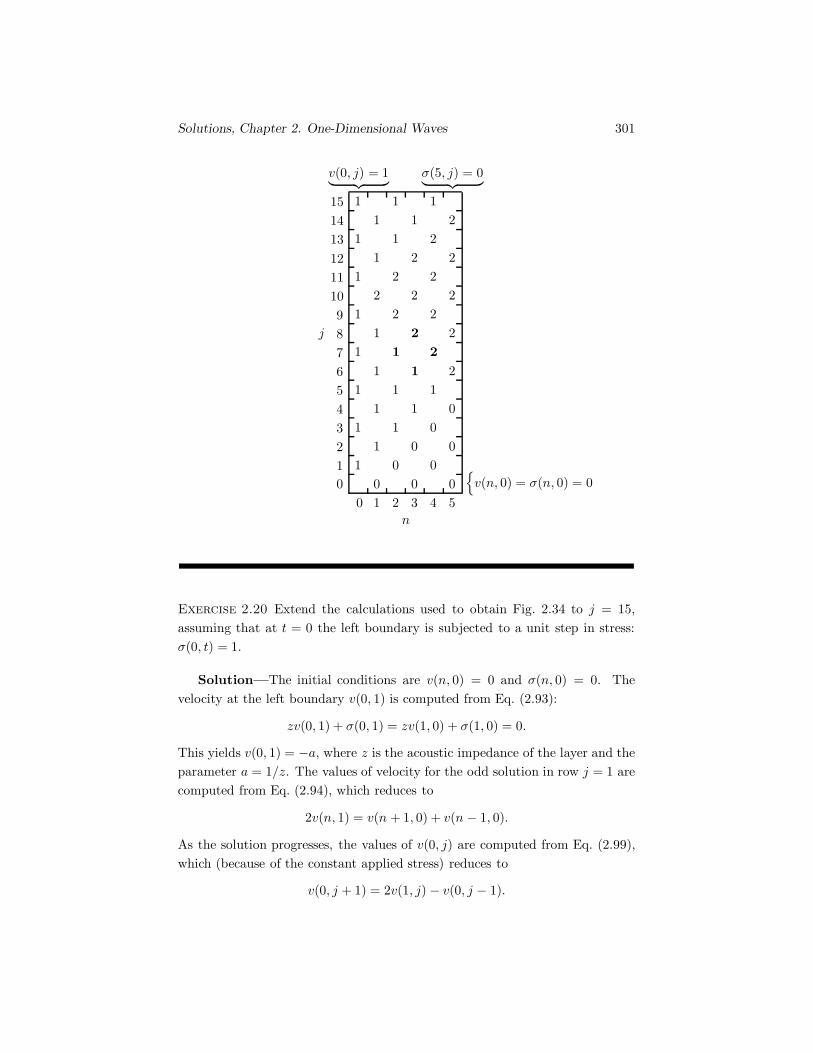
Solutions, Chapter 2. One-Dimensional Waves 301
n
j
v(0, j) = 1︸ ︷︷ ︸ σ(5, j) = 0︸ ︷︷ ︸
{v(n, 0) = σ(n, 0) = 0
0 1 2 3 4 50123456789
101112131415
1
1
1
1
1
1
1
1
1
1
1
1
1
1
1
1
1
1
1
1
1
1
1
1
0
0
0
0
0
0
00
0
2
2
2
2
2
2
2
2
2
2
2
2
2
22
Exercise 2.20 Extend the calculations used to obtain Fig. 2.34 to j = 15,assuming that at t = 0 the left boundary is subjected to a unit step in stress:σ(0, t) = 1.
Solution—The initial conditions are v(n, 0) = 0 and σ(n, 0) = 0. Thevelocity at the left boundary v(0, 1) is computed from Eq. (2.93):
zv(0, 1) + σ(0, 1) = zv(1, 0) + σ(1, 0) = 0.
This yields v(0, 1) = −a, where z is the acoustic impedance of the layer and theparameter a = 1/z. The values of velocity for the odd solution in row j = 1 arecomputed from Eq. (2.94), which reduces to
2v(n, 1) = v(n + 1, 0) + v(n − 1, 0).
As the solution progresses, the values of v(0, j) are computed from Eq. (2.99),which (because of the constant applied stress) reduces to
v(0, j + 1) = 2v(1, j) − v(0, j − 1).

Solutions, Chapter 2. One-Dimensional Waves 302
The values v(5, j) at the stress-free right boundary are computed from Eq. (2.100):
v(5, j + 1) = 2v(4, j) − v(5, j − 1).
The values v(n, j) at the interior points are computed by application of Eq. (2.98).The results are:
n
j
σ(0, j) = 1︸ ︷︷ ︸ σ(5, j) = 0︸ ︷︷ ︸
{v(n, 0) = σ(n, 0) = 0
0 1 2 3 4 50123456789
101112131415
−a
−a
−a
−a
−a
−a
−a
−a
−a
−a
−a
−a
−a
−a−a
00
0
00
0
0
0
0
−3a
−3a
−3a
−3a
−3a−3a
−3a−3a
−3a
−2a−2a
−2a
−2a
−2a
−2a
−2a
−2a
−2a
−2a
−2a
−2a
−2a
−2a
−2a
Exercise 2.21 Repeat the calculations used to obtain Fig. 2.33, replacing theunit step in velocity at the left boundary by the pulse
v(0, j) ={
1 j = 0,0 j > 0.
Solution—Because of the boundary condition, the odd solution (points atwhich n + j is odd) is zero everywhere, and the even solution is computedinstead. The initial conditions are v(n, 0) = 0 for n > 0 and σ(n, 0) = 0 for

Chapter 3. Steady-State Waves 303
all n. The values of the velocity for the even solution in row j = 1 are computedfrom Eq. (2.94), which reduces to
2v(n, 1) = v(n + 1, 0) + v(n − 1, 0).
The boundary conditions for j > 0 are v(0, j) = v(5, j) = 0. The values v(n, j)at the interior points are computed by application of Eq. (2.98). The resultsare:
n
j
v(0, 0) = 1,v(0, j > 0) = 0︸ ︷︷ ︸ σ(5, j) = 0︸ ︷︷ ︸
{v(n > 0, 0) = σ(n, 0) = 0
0 1 2 3 4 50123456789
11
1
1
1
1
1
1
1
0
0
0
0
0
0
0
0
0
00
0
0
0
0
0
0
0
0
0
0
Exercise 2.22 Calculate the results shown in Fig. 2.37.
Solution—Write a program to carry out the algorithm described in exam-ple 4 beginning on page 106.
Solutions, Chapter 3. Steady-State Waves
Exercise 3.1 Show thatu = Aei(kx− ωt)
is a solution of Eq. (3.1) if k = ω/α.

Chapter 3. Steady-State Waves 304
Solution—The second partial derivative of u with respect to t is
∂2u
∂t2=
∂2
∂t2
[Aei(kx − ωt)
]= −ω2Aei(kx − ωt).
The second partial derivative of u with respect to x is
∂2u
∂x2=
∂2
∂x2
[Aei(kx − ωt)
]= −k2Aei(kx − ωt).
Substituting these expressions into Eq. (3.1), the equation is satisfied if k = ω/α.
Exercise 3.2 A half space of elastic material is subjected to the stress bound-ary condition
T11(0, t) = T0e−iωt,
where T0 is a constant. Determine the resulting steady-state displacement fieldin the material.
Solution—The displacement field resulting from this boundary conditionwill be of the form u1 = u1(x1, t), u2 = u3 = 0. For this displacement field, theequations of motion (1.60) reduce to
∂2u1
∂t2= α2∂
2u1
∂x21
.
Assume a solutionu1 = Uei(kx1 − ωt), (∗)
which represents a right-running wave of undetermined constant amplitude U .Substituting this solution into the equation of motion yields
ω2u1 = α2k2u1,
which is satisfied if k = ω/α. From Eq. (1.66) and the stress-strain rela-tion (1.68),
T11 = (λ + 2μ)∂u1
∂x1
= ik(λ + 2μ)Uei(kx1 − ωt).
Chapter 3. Steady-State Waves 305
At the boundary x1 = 0, this is
T11(0, t) = ik(λ+ 2μ)Ue−iωt.
This expression matches the given boundary condition if the constant U is
U =T0
ik(λ+ 2μ).
Substituting this expression into (∗), the displacement field is
u1 =T0
ik(λ + 2μ)ei(kx1 − ωt).
Exercise 3.3 A plate of elastic material of thickness L is subjected to thesteady-state displacement boundary condition
u1(0, t) = Ue−iωt
at the left boundary. The plate is free at the right boundary. Determine theresulting steady-state displacement field in the material.
Solution—Assume a solution consisting of right-running and left-runningwaves:
u1 = Tei(kx1 − ωt) + Rei(−kx1 − ωt),
where T and R are constants and k = ω/α. By evaluating this solution at x1 = 0and equating the result to the displacement applied to the left boundary, weobtain
T +R = U. (∗)
Because the right boundary is stress free, the stress-strain relation gives
T11(L, t) = (λ + 2μ)∂u1
∂x1(L, t) = 0.
Therefore
∂u1
∂x1(L, t) = ikTei(kL − ωt) − ikRei(−kL − ωt) = 0,
which yieldsTeikL −Re−ikL = 0. (∗∗)

Chapter 3. Steady-State Waves 306
Solving Eqs. (∗) and (∗∗) for T and R, we obtain
T =Ue−ikL2 cos kL
, R =UeikL
2 cos kL.
Substituting these expressions into the assumed solution for u1 gives
u1 =U(eikx1e−ikL + e−ikx1eikL)
2 cos kLe−iωt,
which can be written as
u1 =U cos k(x1 − L)
cos kLe−iωt.
Exercise 3.4 A plate of elastic material of thickness L is subjected to thesteady-state shear stress boundary condition
T12(0, t) = T0e−iωt
at the left boundary. The plate is bonded to a rigid material at the right bound-ary. Determine the resulting steady-state displacement field in the material.
Solution—The displacement field resulting from this boundary conditionwill be of the form u2 = u2(x1, t), u1 = u3 = 0. For this displacement field, theequations of motion (1.60) reduce to
∂2u2
∂t2= β2 ∂
2u2
∂x21
.
Assume a solution for the shear displacement consisting of right-running andleft-running waves:
u2 = Tei(kx1 − ωt) + Rei(−kx1 − ωt).
This solution satisfies the equation of motion if k = ω/β. From Eq. (1.66) andthe stress-strain relation (1.68), the stress resulting from the assumed solutionis
T12 = μ∂u2
∂x1
= ikμTei(kx1 − ωt) − ikμRei(−kx1 − ωt).

Chapter 3. Steady-State Waves 307
The boundary condition at x1 = 0 is
T12(0, t) = ikμTe−iωt − ikμRe−iωt = T0e−iωt,
which yields the equation
T − R =−iT0
kμ. (∗)
The boundary condition at x1 = L is
u2(L, t) = Tei(kL − ωt) + Rei(−kL − ωt) = 0,
which yieldsTeikL +Re−ikL = 0. (∗∗)
Solving Eqs. (∗) and (∗∗) for T and!R, we obtain
T =−iT0e
−ikL2kμ cos kL
, R =iT0e
ikL
2kμ cos kL.
Substituting these expressions into the assumed solution for u2 gives
u2 =−iT0(eikx1e−ikL − e−ikx1eikL)
2kμ cos kLe−iωt,
which can be written as
u2 =T0 sin k(x1 − L)
kμ cos kLe−iωt.
Exercise 3.5 A compressional wave is described by the potential
φ = Aei(kx1 cos θ + kx3 sin θ − ωt).
(a) The Lame constants of the material are λ and μ. Determine the stresscomponent T33 as a function of position and time.(b) The density of the material in the reference state is ρ0. Determine thedensity ρ of the material as a function of position and time.

Chapter 3. Steady-State Waves 308
Solution—(a) The components of the displacement are
u1 =∂φ
∂x1= ikφ cos θ,
u2 =∂φ
∂x2= 0,
u3 =∂φ
∂x3= ikφ sin θ.
From the stress-strain relationship (1.68),
T33 = λ
(∂u1
∂x1+∂u2
∂x2+∂u3
∂x3
)+ 2μ
∂u1
∂x1.
Substituting the components of the displacement into this expression, we obtain
T33 = −k2φ(λ+ 2μ sin2 θ).
(b) The relationship between the density and the displacements is given byEq. (1.67):
ρ = ρ0
(1 − ∂u1
∂x1− ∂u2
∂x2− ∂u3
∂x3
).
Substitution of the components of the displacement yields
ρ = ρ0(1 + k2φ).
Exercise 3.6 The motion of an elastic material is described by the displace-ment field
u1 = 0,u2 = u2(x1, x3, t),u3 = 0.
(a) Show that u2 satisfies the wave equation
∂2u2
∂t2= β2
(∂2u2
∂x21
+∂2u2
∂x23
).
For the half-space shown, suppose that the displacement field consists of theincident and reflected waves
u2 = Iei(kx1 cos θ − kx3 sin θ − ωt)
+ Rei(kx1 cos θR + kx3 sin θR − ωt).

Chapter 3. Steady-State Waves 309
(b) Show that k = ω/β.(c) Show that θR = θ and R = I.
Solution—(a) Note that, for the given displacement field,
∂2uk
∂xk∂xm=
∂
∂xm
(∂uk
∂xk
)= 0,
so the equation of motion (1.53) reduces to
∂2um
∂t2= β2 ∂2um
∂xk∂xk,
where β2 = μ/ρ0. For the given displacement field, the equation of motion isidentically zero for m = 1 and m = 3. The desired wave equation is obtainedfrom m = 2.(b) The second partial derivatives of u2 are
∂2u2
∂x21
= −k2 cos2 θIei(kx1 cos θ − kx3 sin θ − ωt)
−k2 cos2 θRRei(kx1 cos θR + kx3 sin θR − ωt),
∂2u2
∂x23
= −k2 sin2 θIei(kx1 cos θ− kx3 sin θ − ωt)
−k2 sin2 θRRei(kx1 cos θR + kx3 sin θR − ωt),
∂2u2
∂x21
= −ω2u2. (∗)
Using these results and the identity
sin2 θ + cos2 θ = 1,
we obtain∂2u2
∂x21
+∂2u2
∂x23
= −k2u2. (∗∗)
Substituting the expressions (∗) and (∗∗) into the wave equation for u2 givesk = ω/β.(c) The surface of the half space is stress free. The components of the unitvector normal to the surface are n1 = 0, n2 = 0, n3 = −1, so from Eq. (ref) thecomponents of the traction vector on the surface are
tk(x1, 0, t) = −Tk3(x1, 0, t) = 0.
Therefore t1(x1, 0, t) = −T13(x1, 0, t) = 0, t2(x1, 0, t) = −T23(x1, 0, t) = 0, andt3(x1, 0, t) = −T33(x1, 0, t) = 0. From Eq. (1.66) and the stress-strain relation
Chapter 3. Steady-State Waves 310
(1.68), the stress components T33 and T13 are identically zero and the componentT23 is
T23 = μ∂u2
∂x3= 0.
Thus the boundary condition at the surface is
∂u2
∂x3(x1, 0, t) = 0,
which yields the equation
I sin θeikx1 cos θ = R sin θReikx1 cos θR .
This equation must hold for all values of x1, which implies that θR = θ andR = I.
Exercise 3.7 Show that in terms of Poisson’s ratio ν , the ratio of the platevelocity cp to the shear wave velocity β is
cpβ
=(
21 − ν
)1/2
.
Solution—Using Eqs. (2.8), (3.60) and (3.62),
c2pβ2
=
[4μ(λ + μ)ρ0(λ+ 2μ)
]μ
ρ0
=4(λ+ μ)λ + 2μ
. (∗)
From Appendix B, the term μ is given in terms of λ and the Poisson’s ratio by
μ =λ(1 − 2ν)
2ν.
Substituting this result into Eq. (*) and simplifying yields the desired result.

Chapter 3. Steady-State Waves 311
Exercise 3.8 Show that in the limit ω → ∞, Eq. (3.58) for the velocities ofthe Rayleigh-Lamb modes becomes identical to Eq. (3.50) for the velocity of aRayleigh wave.
Solution—By reversing the order of the terms raised to the one-half power,we can write Eq. (3.58) as
(2 − c21
β2
)2tan
[i
(β2
c21− 1
)1/2ωh
β
]
tan
[i
(β2
c21− β2
α2
)1/2ωh
β
] − 4(
1 − c21β2
β2
α2
)1/2 (1 − c21
β2
)1/2
= 0.
By using the identity
tan iy =e−y − ey
i(e−y + ey),
we can see that
limω→∞
tan
[i
(β2
c21− 1
)1/2ωh
β
]
tan
[i
(β2
c21− β2
α2
)1/2ωh
β
] = 1,
so that we obtain Eq. (3.50).
Exercise 3.9 Show that in the limit as ω → 0, the solution of Eq. (3.58) forthe velocities of the Rayleigh-Lamb modes is the plate velocity cp.
Solution—We write Eq. (3.58) in the form(2 − c21
β2
)2
tan
[(1 − β2
c21
)1/2ωh
β
]
+4(c21β2
β2
α2− 1
)1/2 (c21β2
− 1)1/2
tan
[(β2
α2− β2
c21
)1/2ωh
β
]= 0.
By expanding the tangents in Taylor series in terms of their arguments, dividingthe equation by ω and then letting ω → 0, we obtain(
2 − c21β2
)2 (1 − β2
c21
)1/2
+ 4(c21α2
− 1)1/2 (
c21β2
− 1)1/2 (
β2
α2− β2
c21
)1/2
= 0.

Chapter 3. Steady-State Waves 312
With some rearrangement and cancellation, this equation reduces to(2 − c21
β2
)2
+ 4(c21α2
− 1)
= 0.
Solving for c1, we obtain
c21 = 4(β2 − β4
α2
).
Setting α2 = (λ + 2μ)/ρ0 and β2 = μ/ρ0, we obtain
c21 =4μ(λ+ μ)ρ0(λ + 2μ)
=Ep
ρ0= c2p.
Exercise 3.10 A wave analogous to a Rayleigh wave can exist at a plane,bonded interface between two different elastic materials. This wave, called aStoneley wave, attenuates exponentially with distance away from the interfacein each material. Derive the characteristic equation for a Stoneley wave.
Solution—Potentials are required for both the upper and lower half spaces.Based on the solution for the phase velocity of Rayleigh waves in Section 3.4,let the potentials in the lower half space be
φ = Ae−hx3ei(k1x1 − ωt),
ψ = Ce−hsx3ei(k1x1 − ωt),
where A and C are constants and
h =(k21 − ω2
α2
)1/2
, hs =(k21 − ω2
β2
)1/2
.
In the upper half space let the potentials be
φ = Ae−hx3ei(k1x1 − ωt),
ψ = Ce−hsx3ei(k1x1 − ωt),
where A and C are constants and
h = −(k21 − ω2
α2
)1/2
, hs = −(k21 − ω2
β2
)1/2
.

Chapter 3. Steady-State Waves 313
The assumed potentials have the same wave number, which is necessary tosatisfy the boundary conditions at the interface. Also, the signs of h, hs, h,and hs have been chosen to yield solutions in both half spaces that decay withdistance from the interface.
The components of displacement in the lower half space are
u1 =∂φ
∂x1− ∂ψ
∂x3
= (ik1Ae−hx3 + hsCe
−hsx3)ei(k1x1 − ωt),
u3 =∂φ
∂x3+∂ψ
∂x1
= (−hAe−hx3 + ik1Ce−hsx3)ei(k1x1 − ωt),
with comparable expressions for the components of displacement u1 and u3 inthe lower half space. The components of displacement in the upper and lowerhalf spaces are equal at x3 = 0:
(u1)x3=0 = (u1)x3=0,
(u3)x3=0 = (u3)x3=0.
Substituting the expressions for the displacement components in terms of thepotentials, these two boundary conditions result in the equations
ik1A+ hsC = ik1A+ hsC,
−hA+ ik1C = −hA + ik1C.
}(∗)
The assumed solutions must also satisfy the stress boundary conditions
(T13)x3=0 = (T13)x3=0,
(T33)x3=0 = (T33)x3=0.
From Eq. (1.66) and the stress-strain relations (1.68),
T13 = μ
(∂u1
∂x3+∂u3
∂x1
),
T33 = λ∂u1
∂x1+ (λ + 2μ)
∂u3
∂x3.
Substituting these relations into the stress boundary conditions and using theexpressions for the displacement components in terms of the potentials togetherwith the relations
λ+ 2μ = ρ0α2 = μ
α2
β2, λ = μ
(α2
β2− 2
),

Chapter 3. Steady-State Waves 314
the stress boundary conditions yield the equations
−2ik1hA− (h2s + k2
1)C = −2ik1hA− (h2s + k2
1)C,
iμ
[α2
β2(k2
1 − h2) − 2k21
]A − 2μk1hsC = iμ
[α2
β2(k2
1 − h2) − 2k21
]A − 2μk1hsC.
⎫⎪⎬⎪⎭ (∗∗)
The four equations (∗) and (∗∗) can be written in the matrix form
[M ]
⎡⎢⎢⎣ACAC
⎤⎥⎥⎦ = [0],
which has a nontrivial solution only if the determinate |M | = 0. In terms of thewave number k1 and frequency ω, the Stonely wave phase is cst = ω/k1. Notefrom the definition of h that
α2
β2(k2
1 − h2) =ω2
β2,
h
k1=
(1 − c2st
α2
)1/2
,hs
k1=
(1 − c2st
β2
)1/2
.
Using these relations, the determinate |M | can be written∣∣∣∣∣∣∣∣∣∣∣∣∣∣∣∣∣∣
1 −(
1 − c2st
β2
)1/2
−1 −(
1 − c2st
β2
)1/2
(1 − c2st
α2
)1/2
−1(
1 − c2st
α2
)1/2
1
2(
1 − c2st
α2
)1/2
−(
2 − c2st
β2
)2μ
μ
(1 − c2st
α2
)1/2μ
μ
(2 − c2st
β2
)(
2 − c2st
β2
)−2
(1 − c2st
β2
)1/2
−μμ
(2 − c2st
β2
)−2
μ
μ
(1 − c2st
β2
)1/2
∣∣∣∣∣∣∣∣∣∣∣∣∣∣∣∣∣∣
= 0.
This equation, which can be solved for the phase velocity cst, is the characteristicequation for a Stonely wave. Notice that the phase velocity does not depend onthe frequency or wave number, but is a function solely of the properties of thetwo materials.
Exercise 3.11 Show that when za = zb, Eq. (3.73) yields the expression givenin Eq. (3.74) for the phase velocity c1 = ω/k in a layered material.

Chapter 3. Steady-State Waves 315
Solution—Setting za = zb in Eq. (3.73) yields
cos kd = cos(ωda
αa
)cos
(ωdb
αb
)− sin
(ωda
αa
)sin
(ωdb
αb
).
By using the identity cos(θ1 +θ2) = cos θ1 cos θ2−sin θ1 sin θ2 , this equation canbe written
cos kd = cos(ωda
αa+ωdb
αb
),
which has solutions
kd =(da
αa+db
αb
)ω + 2πm, m = 0, 1, . . .
The solution for m = 0 is the desired result.
Exercise 3.12 Show that in the limit ω → 0, the solution of Eq. (3.73) for thephase velocity of a steady-state wave in a layered material is given by Eq. (3.75).
Solution—Expressing the sine and cosine terms in Eq. (3.73) as Taylorseries of their arguments and dividing the equation by k2, it can be written
d2 +O(k2) = [Δ2d + O(ω2)]c21, (∗)
where c1 = ω/k is the phase velocity and
Δ2d =
(da
αa
)2
+(za
zb+zb
za
)dadb
αaαb+
(db
αb
)2
.
The notation O(k2) means “terms of order 2 or greater in k.” Solving Eq. (∗)for the phase velocity yields
c1 =[d2 +O(k2)Δ2
d + O(ω2)
]1/2
. (∗∗)
A non-zero limit of c1 = ω/k as ω → 0 exists only if k → 0 as ω → 0. Thereforewe see from Eq. (∗∗) that
limω→0
c1 =d
Δd,
which is Eq. (3.75).
Chapter 3. Steady-State Waves 316
Exercise 3.13 For the layered material discussed in Section 3.6, the fractionof the volume of the material occupied by material a is φ = da/(da +db) = da/d.Derive an equation for the low-frequency limit of the phase velocity as a functionof φ. Using the properties of tungsten for material a and aluminum for material b(see Table B.2 in Appendix B), plot your equation for values of φ from zero toone.
Solution—Noting that φ = da/d and 1−φ = db/d, we can write Eq. (3.76)as
1c21
=φ2
α2a
+(za
zb+zb
za
)φ(1 − φ)αaαb
+(1 − φ)2
α2b
. (∗)
From Table B.2 in Appendix B, the density of tungsten is ρa = 19.4×10³ kg/m3
and its compressional wave velocity is αa = 5.20 × 10³ m/s. Its acousticimpedance is
za = ρaαa
= (19.4× 10³ kg/m3)(5.20 × 103 m/s)
= 1.01× 10⁸ kg/m2s.
The density of aluminum is ρb = 2.70 × 10³ kg/m3 and its compressional wavevelocity is αb = 6.42× 10³ m/s. Its acoustic impedance is
zb = ρbαb
= (2.70× 10³ kg/m3)(6.42× 103 m/s)
= 1.73× 10⁷ kg/m2s.
Using this data, we solve Eq. (∗) for c1 as a function of φ:

Solutions, Chapter 4. Transient Waves 317
0 0.2 0.4 0.6 0.8 14000
4500
5000
5500
6000
6500
φ
c 1,m/s
Notice that there is a range of values of φ for which c1 is less than thecompressional wave velocity in either material.
Chapter 4. Transient Waves
Exercise 4.1 Suppose that an elastic half space is initially undisturbed and issubjected to the velocity boundary condition
∂u1
∂t(0, t) = H(t)e−bt,
where H(t) is the step function and b is a positive real number.(a) By using a Laplace transform with respect to time, show that the solutionfor the Laplace transform of the displacement is
uL1 =
e−sx1/α
s(s+ b).
(b) By inverting the Laplace transform obtained in Part (a), show that thesolution for the displacement is
u1 =1b
[1 − e−b(t − x1/α)
]when t >
x1
α,
u1 = 0 when t <x1
α.

Solutions, Chapter 4. Transient Waves 318
Solution—(a) The Laplace transform of the wave equation for an initially undisturbedmaterial is given by Eq. (4.6):
d2uL1
dx21
− s2
α2uL
1 = 0.
The solution for a wave propagating in the positive x1 direction is
uL1 = Be−sx1/α. (∗)
To determine the constant B in this expression, we evaluate the Laplace trans-form of the boundary condition:∫ ∞
0
∂u1
∂t(0, t)e−st dt =
∫ ∞
0
H(t)e−(s + b)t dt
= − e−(s+ b)t
s+ b
∣∣∣∣∣∞
0
=1
s+ b.
Integrating the left side of this equation by parts,
u1(0, t)e−st∣∣∣∞0
+ s
∫ ∞
0
u1(0, t)e−st dt =1
s+ b,
we obtain(uL
1 )x1=0 =1
s(s + b).
Using this expression to evaluate the constant B in Eq. (∗) gives the desiredresult.(b) The inversion integral (4.1) gives
u1(x1, t) =1
2πi
∫C∞
es(t − x1/α)
s(s+ b)ds.
The integrand
g(s) =1
2πis (s+ b)es(t − x1/α)
has first-order poles at s = 0 and s = −b. By using the closed contour inFig. 4.3.a and evaluating the residues, we obtain
limR→∞
4∑k=1
∫Ck
g(s) ds = lims→0
1s+ b
es(t − x1/α) + lims→−b
1ses(t − x1/α)
=1b
[1 − e−b(t − x1/α)
].

Solutions, Chapter 4. Transient Waves 319
Using the arguments on page 163, the integrals along C2 and C4 approach zero.Jordan’s lemma shows that the integral along C3 also approaches zero providedthat t > x1/α. Therefore
u1(x1, t) =1b
[1 − e−b(t − x1/α)
]when t > x1/α.
When t < x1/α, we can evaluate the displacement using the closed contourshown in Fig. 4.3.b. In this case the contour contains no poles, so the integralover the closed contour is zero and the resulting displacement is zero.
Exercise 4.2 Use Jordan’s lemma to show that
limR→∞
∫CS
12π(b+ iω)2
eiω(t − x1/α) dω = 0 when t >x1
α,
where CS is the semicircular contour shown in Fig. 4.4.b.
Solution—If we let
s = iω, a = t − x1
α, h(s) =
12πi(b+ s)2
,
the integral becomes
I =∫
CS
h(s)eas ds.
Along the contour CS , ω = d+ ie and s = −e+ id, where e and d are real ande ≥ 0. Thus Re(as) = −e(t − x1/α) ≤ 0 when t > x1/α. Also, as R → ∞,h(s) → 1/2πis2, so |h(s)| → 0. Therefore Jordan’s lemma states that I → 0 asR → 0.
Exercise 4.3 Show that when t < x1/α, the solution of Eq. (4.26) is
u1 = limR→∞
∫CR
g(ω) dω = 0.

Solutions, Chapter 4. Transient Waves 320
Solution—From Eq. (4.25),
g(ω) = h(ω)eaω
whereh(ω) =
12π(b+ iω)2
, a = iω(t− x1
α
).
The function g(ω) has a second-order pole at ω = bi.Consider the contour composed of segments CR and C ′
S shown in this exer-cise. It contains no poles, so
limR→∞
∫CR
g(ω) dω + limR→∞
∫C′
S
g(ω) dω = 0.
On C ′S , ω = d− ie, where d and e are real and e ≥ 0. Also on C ′
S , |h(ω)| → 0as R → ∞, and Re(aω) = e(t − x1/α) ≤ 0 provided that t < x1/α. ThereforeJordan’s lemma states that the second integral in the above equation approacheszero as R→ 0, giving the desired result.
Exercise 4.4 Suppose that an unbounded elastic material is subjected to theinitial displacement and velocity fields
u1(x1, 0) = p(x1),
∂u1
∂t(x1, 0) = 0,
where p(x1) is a prescribed function. By taking a Fourier transform with respectto x1 with the transform variable denoted by k, show that the solution for theFourier transform of the displacement is
uF1 = 1
2pF
(e−iαkt + eiαkt
),
where pF is the Fourier transform of the function p(x1).
Solution—We take the Fourier transform of the wave equation with respectto x1 with the transform variable denoted by k:∫ ∞
−∞
∂2u1
∂t2e−ikx1 dx1 =
∫ ∞
−∞α2∂
2u1
∂x21
e−ikx1 dx1.

Solutions, Chapter 4. Transient Waves 321
Integrating the left side by parts twice and using the conditions that u1 and∂u1/∂x1 are zero at x1 = ±∞, we obtain
d2uF1
dt2+ k2α2uF
1 = 0.
The solution of this ordinary differential equation is
uF1 (k, t) = Ae−iαkt + Beαkt.
The initial conditions give
uF1
∣∣t=0
= pF = A+ B
andduF
1
dt
∣∣∣∣t=0
= 0 = −ikαA+ ikαB.
Solving these two equations, we obtain A = B = pF/2, which yields the desiredsolution.
Exercise 4.5 Consider the function of time f(t) = t.(a) If you represent this function as a discrete Fourier series
f(t) =∞∑
n=−∞Ane
iωnt
over the interval 0 ≤ t ≤ 1, show that the coefficients are
An =e−iωn (iωn + 1)
ω2n
− 1ω2
n
. (4.80)
(b) Show that A0 = 1/2.
Solution—(a) The coefficients are
An =∫ 1
0
f(t)e−iωnt dt
=∫ 1
0
te−iωnt dt
=
[e−iωnt
(−iωn)2(−iωn − 1)
]1
0
=e−iωn (iωn + 1)
ω2n
− 1ω2
n
.
Solutions, Chapter 4. Transient Waves 322
(b) The Taylor series of the term e−iωn is
e−iωn = 1 − iωn − 12ω2
n +16iω3
n +O(ω4n),
where O(ω4n) means “terms of order 4 or greater in ωn.” Dividing this expression
by ω2n gives
e−iωn
ω2n
=1ω2
n
− i
ωn− 1
2+
16iωn + O(ω2
n).
Substituting this series into the expression for An gives
An =12
+O(ωn),
so that A0 = 1/2.
Exercise 4.6 Calculate the results shown in Fig. 4.6. Use T = 100 and α = 1.Repeat the calculation using N =256, 128, and 64. What causes the solutionto change?
Discussion—In carrying out these computations, you need to be aware thatimplementations of the FFT vary. Some are specialized to real values of fn, butsome accept complex values. The particular implementation used influencesyour choice of N . Another variation is the placement of the normalizationfactor 1/N ; it can appear in Eq. (4.36) or in Eq. (4.41), with a correspondingaffect on Eq. (4.43).
Solution—The FFT solution is a periodic function over the interval 0 ≤m ≤ N . The dashed lines show the periodic continuations of the solutions.

Solutions, Chapter 4. Transient Waves 323
0 50 100 150 200−0.1
0
0.1
0.2
0.3
0.4
m = t/Δ
Displacement×
bN = 256
0 50 100 150 200−0.1
0
0.1
0.2
0.3
0.4
m = t/Δ
Displacement×
b
N = 128N = 128
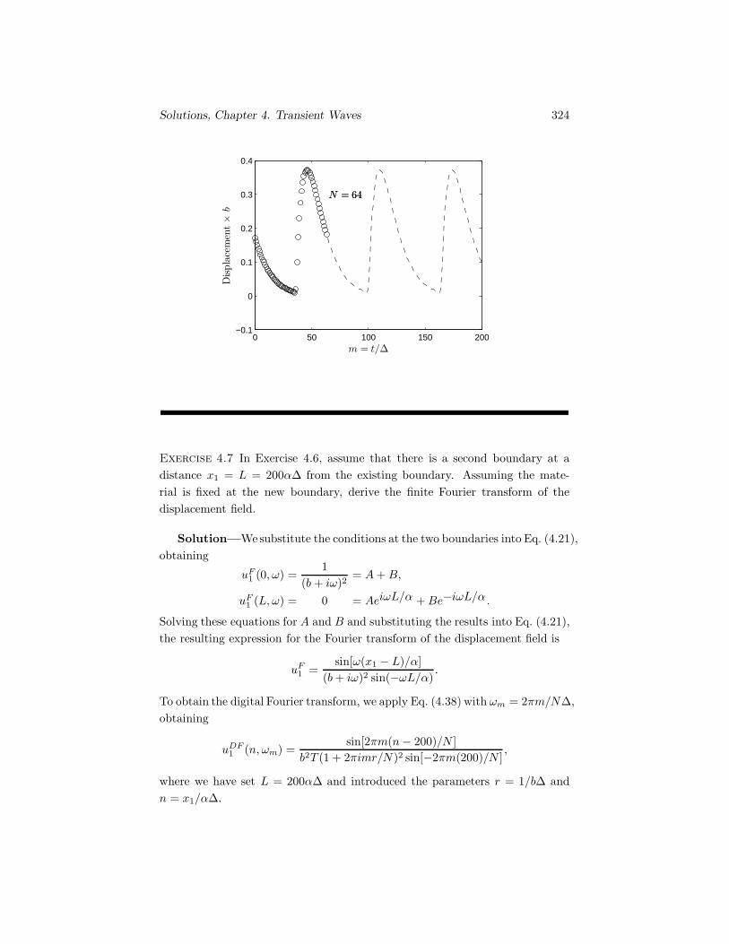
Solutions, Chapter 4. Transient Waves 324
0 50 100 150 200−0.1
0
0.1
0.2
0.3
0.4
m = t/Δ
Displacement×
b
N = 64N = 64
Exercise 4.7 In Exercise 4.6, assume that there is a second boundary at adistance x1 = L = 200αΔ from the existing boundary. Assuming the mate-rial is fixed at the new boundary, derive the finite Fourier transform of thedisplacement field.
Solution—Wesubstitute the conditions at the two boundaries into Eq. (4.21),obtaining
uF1 (0, ω) =
1(b + iω)2
= A+ B,
uF1 (L, ω) = 0 = AeiωL/α +Be−iωL/α.
Solving these equations for A and B and substituting the results into Eq. (4.21),the resulting expression for the Fourier transform of the displacement field is
uF1 =
sin[ω(x1 − L)/α](b+ iω)2 sin(−ωL/α)
.
To obtain the digital Fourier transform, we apply Eq. (4.38) with ωm = 2πm/NΔ,obtaining
uDF1 (n, ωm) =
sin[2πm(n− 200)/N ]b2T (1 + 2πimr/N)2 sin[−2πm(200)/N ]
,
where we have set L = 200αΔ and introduced the parameters r = 1/bΔ andn = x1/αΔ.

Solutions, Chapter 4. Transient Waves 325
Exercise 4.8 The discrete Fourier transform converts N real numbers into Ncomplex numbers. Use the properties of periodicity and symmetry of fDF
n toshow that half of the values of the fDF
n are sufficient to determine the otherhalf.
Solution—From the definition of the discrete Fourier transform, Eq. (4.36),we obtain
fDF−m =
1N
N−1∑n=0
fne2πimn/N .
Because fn is real, the complex conjugate of fDF−m is
fDF−m =
1N
N−1∑n=0
fne−2πimn/N = fDF
−m . (∗)
Application of the periodicity condition (4.37) gives
fDFN−m = fDF
m .
For m = 1, 2, . . . , N − 1, half of the values of fDFm are equal to the complex
conjugates of the other half. For the case m = 0, Eq. (*) gives fDF0 = fDF
0 .Thus
Im(fDF0 ) = 0.
Consequently, of the 2N real numbers representing the N complex values offDF
m , one of them is zero and N − 1 other values are negatives of the remainingnumbers.
Exercise 4.9 Show that the group velocity cg = dω/dk is related to the phasevelocity c1 by
cg = c1 + k1dc1dk1
=c1
1 − ω
c1
dc1dω
.
Solution—Beginning with the definition c1 = ω/k1, we obtain
dc1dk1
=1k1
dω
dk1− ω
k21
=1k1
(cg − c1),

Solutions, Chapter 4. Transient Waves 326
which yields the first result. Similarly,
dc1dω
=1k1
− ω
k21
dk1
dω=
1k1
(1 − c1
cg
),
which yields the second result.
Exercise 4.10 In Section 3.5, we analyzed acoustic waves in a channel.(a) Show that the group velocity of such waves is related to the phase velocityby cgc1 = α2.(b) What is the maximum value of the group velocity?
Solution—(a) We write the dispersion relation, Eq. (3.54), in the form
k21α
2 = ω2 −(αnπ
h
)2
.
The derivative of this expression with respect to k1 yields
k1α2 = ω
dω
dk1,
orα2 = c1cg. (∗)
(b) By substituting Eq. (3.54) into the relation (∗), we obtain
cg =α2
c1= α
[1 −
(αnπωh
)2]1/2
.
For frequencies above the cutoff frequency, 1 ≥ 1 − (αnπ/ωh)2 ≥ 0. Therefore
cg ≤ α.
For frequencies below the cutoff frequency, c1 and cg are imaginary and thesolution does not describe a propagating wave.

Solutions, Chapter 4. Transient Waves 327
Exercise 4.11 Use Eq. (3.73) to derive an expression for the group velocity ofa layered medium with periodic layers.
Solution—Differentiation of Eq. (3.73) with respect to k yields
d sin(kd) =dω
dk
{da
αasin
(ωda
αa
)cos
(ωdb
αb
)+db
αbcos
(ωda
αa
)sin
(ωdb
αb
)
+12
(za
zb+zb
za
)[da
αacos
(ωda
αa
)sin
(ωdb
αb
)
+db
αbsin
(ωda
αa
)cos
(ωdb
αb
)]}.
Solving for dω/dk = cg and rearranging terms yields
cg = d sin(kd)/{[
da
αa+
12
(za
zb+zb
za
)db
αb
]sin
(ωda
αa
)cos
(ωdb
αb
)
+[db
αb+
12
(za
zb+zb
za
)da
αa
]cos
(ωda
αa
)sin
(ωdb
αb
)}.
Exercise 4.12 Use the result of Exercise 4.11 to show that the group velocityis zero at the edges of a pass band.
Solution—In Fig. 3.32, the edges of the pass bands separate intervalswhere k is real from intervals where k is complex. From the dispersion re-lation (3.73), the boundaries between real and complex solutions are wherecos(kd) = ±1. At these values of k, sin(kd) = 0. Provided the denominator ofthe result for cg from Exercise 4.11 is not zero, cg is zero at the edges of thepass bands.
Exercise 4.13 Consider Lamb’s problem for an acoustic medium. (See thediscussion of an acoustic medium on page 44.) Use the Cagniard-de Hoopmethod to show that the solution for the stress component T33 is
T33 = −T0
πH
(t− r
α
) sin θ
r
(1 − r2
t2α2
)1/2.

Solutions, Chapter 4. Transient Waves 328
Solution—An acoustic medium is a linear elastic material with zero shearmodulus (μ = 0). This exercise requires modifying the solution of Lamb’sproblem presented in Section 4.5 to the case of an acoustic medium.
Because μ = 0, the Helmholtz decomposition is
u = ∇φ,
and, from Eqs. (4.53) and (4.55),
T33 = λ
(∂u1
∂x1+∂u3
∂x3
)= λ
(∂2φ
∂x21
+∂2φ
∂x23
). (1)
From Eq. (4.56), the wave equation satisfied by φ is
∂2φ
∂t2= α2
(∂2φ
∂x21
+∂2φ
∂x23
). (2)
The Laplace transform of the potential φ is
φL =∫ ∞
0
φe−st dt,
and the Fourier transform of φL with respect to x3 is defined to be
φLF =∫ ∞
−∞φLe−iksx1 dx1.
From Eq. (4.61) and the discussion that follows it, applying the Laplace andFourier transforms to the wave equation (2) leads to the solution
φLF = Ae−(k2 + v2P )1/2sx3 ,
where A is a constant and vP = 1/α is the compressional “showness.” FromEq. (4.62), applying the Laplace and Fourier transforms to the normal stressboundary condition leads to the equation[
d2φLF
dx23
− k2s2φLF
]x3=0
= −T0
λs.
Using this equation to solve for A, we obtain the solution for φLF :
φLF = − T0
λs3v2P
e−(k2 + v2P )1/2sx3 .
We apply the Fourier inversion integral to this expression:
φL = − 12π
∫ ∞
−∞
T0
λs2v2P
e−[(k2 + v2P )1/2x3 − ikx1]s dk.

Solutions, Chapter 5. Nonlinear Wave Propagation 329
We substitute this result into the Laplace transform of Eq. (1), obtaining
TL33 = −T0
2π
∫ ∞
−∞e−[(k2 + v2
P )1/2x3 − ikx1]s dk. (3)
To evaluate this integral, we define a real parameter t by
t = (k2 + v2P )1/2x3 − ikx1.
From Eq. (4.66), the solutions for k in terms of t are
k± =it
rcos θ ±
(t2
r2− v2
P
)1/2
sin θ. (4)
As the value of the parameter t goes from vP r to ∞, the values of k given bythis equation describe the two paths B− and B+ in the complex k-plane shownin Fig. 4.27.
The integrand of Eq. (3) has branch points at k = ±vP i but no poles. Thediscussion on page 200 applies to this integral. Consequently, the integrationalong the path C1 can be replaced by integration along the paths B− and B+:
TL33 = −T0
2π
[∫ ∞
vP r
e−st ∂k+
∂tdt−
∫ ∞
vP r
e−st ∂k−∂t
dt
].
By introducing the step function H(t−vP r), the lower limits of integration canbe changed to zero:
TL33 = −T0
2π
∫ ∞
0
H(t − vP r)(∂k+
∂t− ∂k−
∂t
)e−st dt.
Because the parameter s appears only in the exponential term, this integralmatches the definition of the Laplace transform. Therefore
T33 = −T0
2πH(t− vP r)
(∂k+
∂t− ∂k−
∂t
).
From Eq. (4),∂k+
∂t− ∂k−
∂t=
2t sin θ
r2(t2
r2− v2
P
)1/2,
which completes the solution.
Chapter 5. Nonlinear Wave Propagation
Exercise 5.1 Consider the one-dimensional linear wave equation
∂2u
∂t2= α2∂
2u
∂x2,

Solutions, Chapter 5. Nonlinear Wave Propagation 330
where α is constant. Introducing the variables v = ∂u/∂t and w = ∂u/∂x, itcan be written as the system of first-order equations
∂v
∂t= α2∂w
∂x,
∂v
∂x=
∂w
∂t.
(a) Use Eq. (5.21) to show that there are two families of right-running and left-running characteristics in the x-t plane and that the characteristics are straightlines.(b) Show that the system of first-order equations is hyperbolic.
Solution—(a) Express the system of first-order equations in the form of Eq. (5.17) byletting
uk =[vw
], Akm =
[1 00 1
], Bkm =
[0 −α2
−1 0
].
Equation (5.21) becomes [c α2
1 c
]= 0,
which has the rootsc = ±α.
Because α is a constant, the characteristics are straight lines.(b) Equation (5.27) becomes[
c 1α2 c
] [r1r2
]= 0.
There are two solutions for the vector r:
r2 = −αr1 for c = α
andr2 = αr1 for c = −α.
The system is hyperbolic because the roots c are real and two linearly indepen-dent vectors r exist.
Solutions, Chapter 5. Nonlinear Wave Propagation 331
Exercise 5.2 Consider the system of first-order equations in Exercise 5.1. Usethe interior equation, Eq. (5.26), to show that v−αw is constant along a right-running characteristic and v+αw is constant along a left-running characteristic.
Solution—For a right-running characteristic, c = α and r2 = −αr1. Theinterior equation for this characteristic is
r1[
1 − α] [ ζt −α2ζx
−ζx ζt
] [vζ
wζ
],
which can be written(v − αw)ζ dζ = 0.
Along a right-running characteristic, dη = 0, and consequently
d(v − αw) = (v − αw)ζ dζ = 0.
Therefore v−αw is constant along a right-running characteristic. Use the sameargument to show that v + αw is constant along a left-running characteristic,for which c = −α and r2 = αr1.
Exercise 5.3 Consider the simple wave solution beginning on page 224. Sup-pose that the relationship between the stress and the deformation gradient isT (F ) = E0 lnF , where E0 is a constant.(a) Show that within the characteristic fan, the velocity is given in terms of thedeformation gradient by
v = −2α0(F 1/2 − 1),
where α0 = (E0/ρ0)1/2.(b) Show that within the characteristic fan, the deformation gradient and ve-locity are given as functions of X, t by
F =α2
0t2
X2, v = −2α0
(α0t
X− 1)
).
Solution—(a) The derivative of the stress with respect to the deformation gradient is
TF =E0
F,

Solutions, Chapter 5. Nonlinear Wave Propagation 332
therefore
α =
(TF
ρ0
)1/2
=α0
F 1/2. (∗)
Substitution of this expression into Eq. (5.30) gives
v = −2α0(F 1/2 − 1).
(b) Because each characteristic within the fan is a straight line through theorigin, α = X/t. From Eq. (∗),
F =α2
0
α2=α2
0t2
X2.
Substituting this expression into the answer to Part (a) yields the desired result.
Exercise 5.4 A half space of elastic material is initially undisturbed. At t = 0the boundary is subjected to a uniform constant stress T0. The stress is relatedto the deformation gradient by the logarithmic expression T = T (F ) = E0 lnF ,where E0 is a constant. Show that the resulting velocity of the boundary of thehalf space toward the left is(
E0
ρ0
)1/2 [e(T0/2E0) − 1
].
Solution—In Fig. 5.10, the characteristic fan separates region 1 from region2. The stress T and deformation gradient F in region 2 are determined by theapplied stress:
T = E0 lnF = T0.
We solve for F ,F = eT0/E0 ,
and substitute this result into the expression for v from Part (a) of Exercise 5.3,obtaining
v = −(E0
ρ0
)1/2 [e(T0/2E0) − 1
].

Solutions, Chapter 5. Nonlinear Wave Propagation 333
Exercise 5.5 Consider a weak wave propagating into an undisturbed nonlinearelastic material. Show that the equation governing the rate of change of thediscontinuity in vX is
d
dt[[vX]] =
(TFF
2ρ0α20
)[[vX ]]2.
Solution—Applying the chain rule,
vX = ηXvη + ζXvζ .
Letting ζ = t and η = t−X/α0 in this equation, we obtain
vη = −α0vX .
Substitution of this expression into Eq. (5.36) yields the desired result.
Exercise 5.6 (a) Determine the relation T = T (F ) for a linear elastic material.(b) What is the velocity of an acceleration wave in a linear elastic material?(c) What is the velocity of a shock wave in a linear elastic material?
Solution—(a) In one-dimensional motion of a linear elastic material, the density is relatedto the longitudinal strain by
ρ0
ρ= 1 +E11,
soE11 =
ρ0
ρ− 1 = F − 1,
and the stress-strain relation is
T11 = (λ+ 2μ)E11.
ThereforeT = T (F ) = (λ + 2μ)(F − 1). (∗)

Solutions, Chapter 5. Nonlinear Wave Propagation 334
(b) From Eq. (∗), TF = dT/dF = λ+ 2μ. Then from Eq. (5.48), the velocity ofan acceleration wave is
vs =
(TF
ρ0
)1/2
=(λ+ 2μρ0
)1/2
.
(c) From Eq. (∗), [[T ]] = (λ + 2μ)[[F ]]. Then from Eq. (5.56), the velocity of ashock wave is
vs =(
[[T ]]ρ0[[F ]]
)1/2
=(λ + 2μρ0
)1/2
.
Exercise 5.7 The relation between the stress and the deformation gradient ina material is T = T (F ) = E0 lnF , where E0 is a constant. The density of theundeformed material is ρ0.(a) What is the velocity of an acceleration wave in the undeformed material?(b) If the material is homogeneously compressed so that its density is 2ρ0, whatis the velocity of an acceleration wave?
Solution—(a) The velocity of an acceleration wave is
vs =
(TF
ρ0
)1/2
=(E0
ρ0F
)1/2
. (∗)
The deformation gradient in the undisturbed material ahead of the wave isF = 1. Consequently, in the undisturbed material
vs =(E0
ρ0
)1/2
.
(b) In a material compressed to 2ρ0, F = 1/2. From Eq. (∗), the velocity is
vs =(
2E0
ρ0
)1/2
.

Solutions, Chapter 5. Nonlinear Wave Propagation 335
Exercise 5.8 The relation between the stress and the deformation gradientin a material is T = T (F ) = E0 lnF , where E0 is a constant. The densityof the undeformed material is ρ0. An acceleration wave propagates into theundeformed material. At t = 0, the acceleration of the material just behindthe wave is a0 in the direction of propagation. What is the acceleration of thematerial just behind the wave at time t?
Solution—Because F is continuous across an acceleration wave, F = 1 justbehind the wave. The growth of the amplitude of the wave is given by Eq. (5.53):
d
dt
[[∂v
∂t
]]= − TFF
2ρ0v3s
[[∂v
∂t
]]2
=1
2(E0/ρ0)1/2
[[∂v
∂t
]]2
.
Integrating this equation with respect to time yields[[∂v
∂t
]]−1
=−t
2(E0/ρ0)1/2+
1a0,
which after rearrangement yields the result.
Exercise 5.9 If a gas behaves isentropically, the relation between the pressureand the density is
p
ργ=p0
ργ0
,
where γ, the ratio of specific heats, is a positive constant. In the one-dimensionalproblems we are discussing, the stress T = −p.(a) Show that the velocity of an acceleration wave propagating into undisturbedgas with pressure p0 and density ρ0 is
vs =(γp0
ρ0
)1/2
.
(b) If the amplitude [[∂v/∂t]] of an acceleration wave propagating into undis-turbed gas with pressure p0 and density ρ0 is positive, show that the amplitudewill increase with time.
Solution—(a) Expressing the isentropic relation in terms of the stress T =−p and F = ρ0/ρ, we obtain
T = T (F ) = −p0F−γ .
Solutions, Chapter 5. Nonlinear Wave Propagation 336
Therefore
TF =dT
dF= γp0F
−(γ+1). (∗)
At the wavefront, ρ = ρ0, so F = 1 and TF = γp0. Therefore the accelerationwave velocity is
vs =
(TF
ρ0
)1/2
=(γp0
ρ0
)1/2
.
(b) From Eq. (∗),TFF = −(γ + 1)γp0F
−(γ+2).
At the wavefront, TFF = −(γ + 1)γp0 . Because TFF is negative, Eq. (5.53)indicates that the rate of change of [[∂v/∂t]] with respect to time is positive.
Exercise 5.10 The relation between the stress and the deformation gradientin a material is T = T (F ) = E0 lnF , where E0 is a constant. The density ofthe undeformed material is ρ0. A shock wave propagates into the undeformedmaterial. If the density of the material just behind the wave is 2ρ0 at a particulartime, show that the velocity of the wave at that time is
vs =[2E0 ln 2ρ0
]1/2
.
Solution—The velocity of a shock wave is given by Eq. (5.56):
vs =(
[[T ]]ρ0[[F ]]
)1/2
.
In the undisturbed material, F = 1 and T = 0. Behind the shock wave, F =ρ0/2ρ0 = 1/2 and T = E0 ln(1/2). Therefore
vs =[E0 ln(1/2)−ρ0/2
]1/2
.

Solutions, Chapter 5. Nonlinear Wave Propagation 337
Exercise 5.11 The stress-strain relation of an elastic material is given by thesolid curve. The point labeled (−) is the state ahead of a shock wave and thepoint labeled (+) is the state just behind the wave at a time t. Determinewhether [[F ]] will increase, remain the same, or decrease as a function of time incases (a), (b), and (c).
Solution—From Eq. (5.56),
ρ0v2s =
[[T ]][[F ]]
=T− − T+
F− − F+.
The expression on the right is the slope of the dashed straight line from point (+)to point (−). The term (TF )+ in Eq. (5.61) is the slope of the solid curve atpoint (+), which is greater than the slope of the dashed straight line. Thereforethe term
(TF )+ − ρ0v2s
in Eq. (5.61) is positive. In cases (a), (b), and (c), [[∂F/∂X]] is positive, zero,and negative, respectively, so Eq. (5.61) indicates that [[F ]] will decrease withtime in case (a), remain constant in case (b), and increase with time in case c.(Because F+ is negative, notice that this means that the magnitude of the jumpin F will increase with time in case (a), remain constant in case (b), and decreasewith time in case (c).)
Exercise 5.12 Consider a flyer plate experiment in which the flyer plate andthe target are identical materials with mass density 2.79 Mg/m3, the measuredshock wave velocity is 6.66 km/s, and the measured flyer-plate velocity is 2 km/s.What is the pressure in the equilibrium region behind the loading wave?
Solution—From Eqs. (5.72), the pressure in the equilibrium region behindthe loading wave can be expressed as pe = ρ0Uve, where U is the shock wavevelocity and ve is the velocity of the material behind the loading wave. Becausethe flyer plate and the target are identical materials, the Hugoniot curves inFig. 5.22 intersect at vT = v0/2 = 1 km/s. Another way to obtain this result isto view the experiment using a reference frame that is moving to the right withvelocity v0/2. Relative to this reference, the flyer plate and the target approacheach other with the same velocity v0/2. Because the flyer plate and the target

Solutions, Chapter 5. Nonlinear Wave Propagation 338
consist of the same material, the velocity of the materials behind the loadingwaves must be zero. Then if we revert to the fixed reference frame, the velocityof the target material behind the loading wave is v0/2. Therefore, the pressureof the material behind the loading wave is
pe = ρ0Uve
= (2.79× 10³ kg/m3)(6660 m/s)(1000 m/s)
= 18.6× 10⁹ Pa (18.6 GPa).
Exercise 5.13 (a) Consider a flyer plate experiment in which the flyer plate isaluminum with properties ρ0 = 2.79 Mg/m2, c = 5.33 km/s, and s = 1.40, thetarget is stainless steel with properties ρ0 = 7.90 Mg/m2, c = 4.57 km/s, ands = 1.49, and the velocity of the flyer plate is 2 km/s. What is the pressure inboth materials in the equilibrium region behind the loading waves, and what isthe velocity of their interface?(b) If the materials are interchanged so that the flyer plate is stainless steel andthe target is aluminum, what is the pressure in both materials in the equilibriumregion behind the loading waves and what is the velocity of their interface?
Solution—(a) We use Eq. (5.74) to obtain the graph of pT as a function of vT (the Hugo-niot) for the stainless steel target. We use Eqs. (5.75) and (5.77) to obtainthe graph of pF as a function of vT for the aluminum flyer plate, obtaining
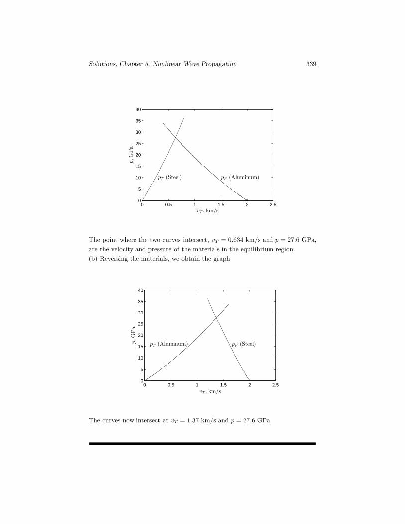
Solutions, Chapter 5. Nonlinear Wave Propagation 339
0 0.5 1 1.5 2 2.50
5
10
15
20
25
30
35
40
vT , km/s
p,GPa
pT (Steel) pF (Aluminum)
The point where the two curves intersect, vT = 0.634 km/s and p = 27.6 GPa,are the velocity and pressure of the materials in the equilibrium region.(b) Reversing the materials, we obtain the graph
0 0.5 1 1.5 2 2.50
5
10
15
20
25
30
35
40
vT , km/s
p,GPa
pT (Aluminum) pF (Steel)
The curves now intersect at vT = 1.37 km/s and p = 27.6 GPa
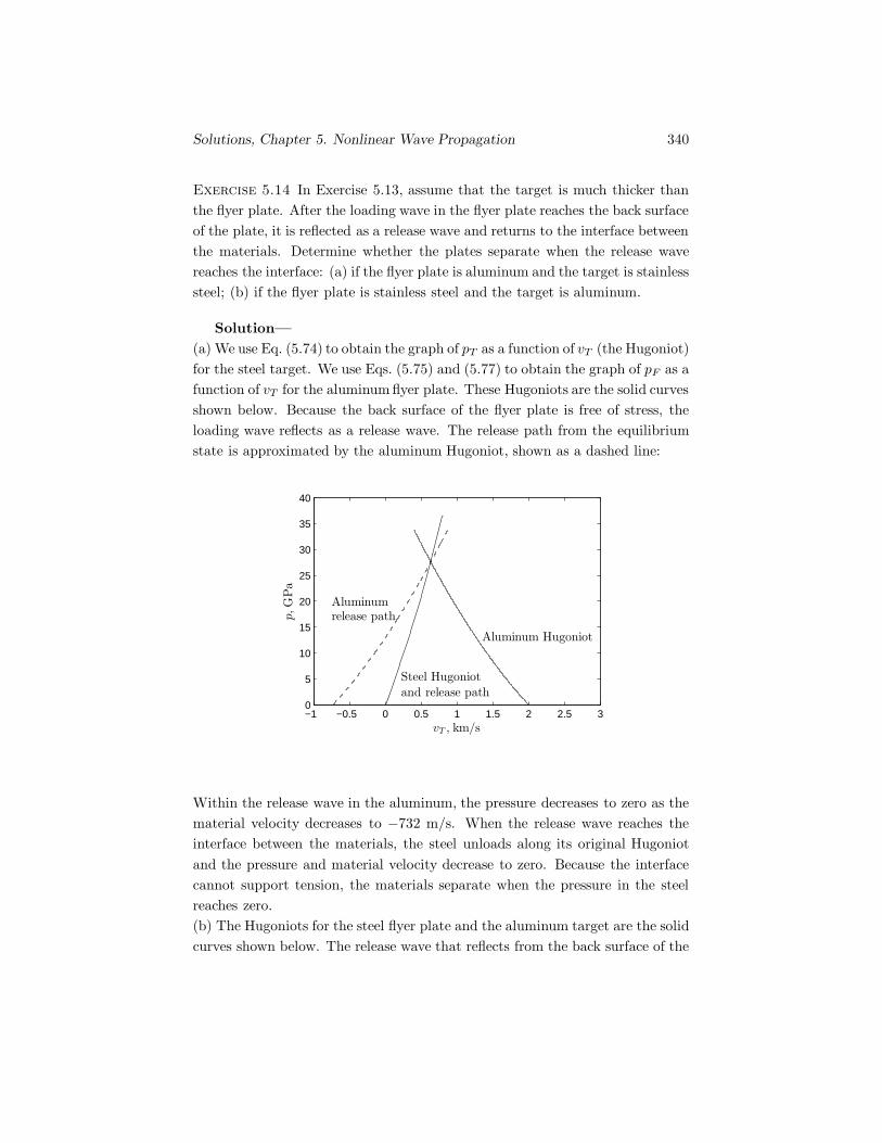
Solutions, Chapter 5. Nonlinear Wave Propagation 340
Exercise 5.14 In Exercise 5.13, assume that the target is much thicker thanthe flyer plate. After the loading wave in the flyer plate reaches the back surfaceof the plate, it is reflected as a release wave and returns to the interface betweenthe materials. Determine whether the plates separate when the release wavereaches the interface: (a) if the flyer plate is aluminum and the target is stainlesssteel; (b) if the flyer plate is stainless steel and the target is aluminum.
Solution—(a) We use Eq. (5.74) to obtain the graph of pT as a function of vT (the Hugoniot)for the steel target. We use Eqs. (5.75) and (5.77) to obtain the graph of pF as afunction of vT for the aluminum flyer plate. These Hugoniots are the solid curvesshown below. Because the back surface of the flyer plate is free of stress, theloading wave reflects as a release wave. The release path from the equilibriumstate is approximated by the aluminum Hugoniot, shown as a dashed line:
−1 −0.5 0 0.5 1 1.5 2 2.5 30
5
10
15
20
25
30
35
40
vT , km/s
p,GPa
Steel Hugoniot
and release path
Aluminum Hugoniot
Aluminumrelease path
Within the release wave in the aluminum, the pressure decreases to zero as thematerial velocity decreases to −732 m/s. When the release wave reaches theinterface between the materials, the steel unloads along its original Hugoniotand the pressure and material velocity decrease to zero. Because the interfacecannot support tension, the materials separate when the pressure in the steelreaches zero.(b) The Hugoniots for the steel flyer plate and the aluminum target are the solidcurves shown below. The release wave that reflects from the back surface of the

Solutions, Appendix A. Complex Analysis 341
flyer plate causes the pressure in the steel to decrease to zero and the velocityto decrease to 732 m/s. When the release wave reaches the interface betweenthe materials, the aluminum unloads along its Hugoniot. However, because thesteel is moving toward the aluminum target at 732 m/s, the pressure in thealuminum does not drop to zero. The target and flyer plate remain in contact,a partial release wave continues into the aluminum, and a reloading wave isformed in the steel. Because the release wave spreads as it travels from the freeleft surface of the aluminum plate to the interface, the reloading wave in thesteel is not a shock wave and approximately follows the steel Hugoniot shown.
0 0.5 1 1.5 2 2.50
5
10
15
20
25
30
35
40
vT , km/s
p,GPa Aluminum Hugoniot
and release
Steel Hugoniot
Steel release
Steel reloading
Appendix A. Complex Analysis
Exercise A.1 Show that the magnitude of a complex variable z is given bythe relation
|z| = (zz)1/2.
Solution—(zz)1/2 = [(x+ iy)(x − iy)]1/2
= (x2 − i2y2)1/2
= (x2 + y2)1/2
= |z|.

Solutions, Appendix A. Complex Analysis 342
Exercise A.2 Show that for any two complex numbers z1 and z2,
|z1z2| = |z1||z2| and∣∣∣∣z1z2
∣∣∣∣ =|z1||z2|
.
Solution—Consider the polar form of a complex variable
z = reiθ = r(cos θ + i sin θ).
Its magnitude is|reiθ| = |r cos θ + ir sin θ|
= (r2 cos2 θ + r2 sin2 θ)1/2
= r.
Using that result, we express z1 and z2 in polar form and obtain
|z1||z2| = |r1eiθ1 ||r2eiθ2 | = r1r2,
|z1z2| = |r1r2ei(θ1 + θ2)| = r1r2,
and|z1||z2|
=|r1eiθ1 ||r2eiθ2 |
=r1r2,∣∣∣∣z1z2
∣∣∣∣ =∣∣∣∣r1r2 ei(θ1 − θ2)
∣∣∣∣ =r1r2.
Exercise A.3
(a) Show that the exponential function f(z) = ez is analytic.(b) Show that the function f(z) = z is not analytic anywhere.
Solution—(a) Letting z = x+ iy, the exponential function can be written
ez = ex(cos y + i sin y).
Its real and imaginary parts are
u = ex cos y, v = ex sin y.
Solutions, Appendix A. Complex Analysis 343
Evaluating their partial derivatives,
∂u
∂x= ex cos y,
∂u
∂y= −ex sin y,
∂v
∂x= ex sin y,
∂v
∂y= ex cos y,
we see that∂u
∂x=∂v
∂y,
∂u
∂y= −∂v
∂x.
Thus the Cauchy-Riemann equations hold for all values of z, so the exponentialfunction is analytic everywhere.(b) The real and imaginary parts of the conjugate function f(z) = z are
u = x, v = −y.
Their partial derivatives are
∂u
∂x= 1,
∂u
∂y= 0,
∂v
∂x= 0,
∂v
∂y= −1.
Consequently,∂u
∂x�= ∂v
∂y,
∂u
∂y= −∂v
∂x.
The Cauchy-Riemann equations do not hold for any value of z, so the conjugatefunction is not analytic everywhere.
Exercise A.4 Evaluate the contour integral∫C
(1 + z) dz
along the contour shown from the point z = 0 to the point z = 1 + i. Compareyour result with the result of the example on page 357.
Solution—Consider two contours:

Solutions, Appendix A. Complex Analysis 344
x
y
1 + i
C1
C2Ce�
�
����
��
The contour C1 + C2 is the integration path for this exercise. The contour Ce
is the integration path in the example on page 357.Expressing the integrand in terms of its real and imaginary parts, for any
path C, ∫C
(1 + z) dz =∫
C
[(1 + x)dx− y dy] + i
∫C
[y dx+ (1 + x)dy].
To integrate along the path C1 +C2, we note that y = 0 on C1 and x = 1 on C2,obtaining ∫
C1+C2
(1 + z) dz =∫ 1
0
(1 + x) dx−∫ 1
0
y dy + i
∫ 1
0
2dy
=(x+
x
2
)∣∣∣10− y2
2
∣∣∣∣10
+ 2y|10
= 1 + 2i.
This is the same value we obtained on page 357 for integration along the pathCe.This result is confirmed by the Cauchy integral theorem. Because the integrand1 + z is analytic and C1, C2 and Ce form a piecewise-smooth closed contour,the theorem states that∫
C1
(1 + z) dz +∫
C2
(1 + z) dz −∫
Ce
(1 + z) dz = 0.
Exercise A.5
(a) Show that the function
f(z) =1
z − 1has a first-order pole at z = 1.(b) Show that the function
f(z) =1
(z − 1)2
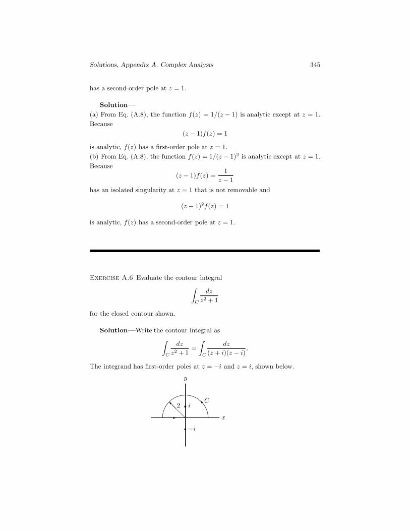
Solutions, Appendix A. Complex Analysis 345
has a second-order pole at z = 1.
Solution—(a) From Eq. (A.8), the function f(z) = 1/(z − 1) is analytic except at z = 1.Because
(z − 1)f(z) = 1
is analytic, f(z) has a first-order pole at z = 1.(b) From Eq. (A.8), the function f(z) = 1/(z − 1)2 is analytic except at z = 1.Because
(z − 1)f(z) =1
z − 1has an isolated singularity at z = 1 that is not removable and
(z − 1)2f(z) = 1
is analytic, f(z) has a second-order pole at z = 1.
Exercise A.6 Evaluate the contour integral∫C
dz
z2 + 1
for the closed contour shown.
Solution—Write the contour integral as∫C
dz
z2 + 1=
∫C
dz
(z + i)(z − i).
The integrand has first-order poles at z = −i and z = i, shown below.
x
y
2C
i
−i
�� ........
........
.............................................
........................
........................................................................................................................................................................................ �
��' '
�

Solutions, Appendix A. Complex Analysis 346
Only the pole at z = i is within the closed contour. Its residue is
limz→i
(1
z + i
)=
12i.
The value of the contour integral is 2πi times the sum of the residues of thepoles enclosed by the contour:∫
C
dz
z2 + 1= 2πi
(12i
)= π.
Exercise A.7 Evaluate the contour integral∫C
dz
z(z − 1)(z − 3)2
for the closed circular contour shown.
Solution—The integrand has poles at z = 0, z = 1, and z = 3, shownbelow. Only the first-order poles at z = 0 and z = 1 are within the closedcontour.
x
y
2C
0 1 3� � �........
........
.............................................
........................
.................................................................................................................................................................................................................................................................................................................................................................................
...................................................................................�
��' '
The residue of the pole at z = 0 is
limz→0
[1
(z − 1)(z − 3)2
]= −1
9.
The residue of the pole at z = 1 is
limz→1
[1
z(z − 3)2
]=
14.
The value of the contour integral is 2πi times the sum of the residues of thepoles enclosed by the contour:∫
C
dz
z(z − 1)(z − 3)2= 2πi
(14− 1
9
)=
518πi.
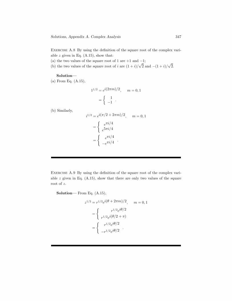
Solutions, Appendix A. Complex Analysis 347
Exercise A.8 By using the definition of the square root of the complex vari-able z given in Eq. (A.15), show that:(a) the two values of the square root of 1 are +1 and −1;(b) the two values of the square root of i are (1 + i)/
√2 and −(1 + i)/
√2.
Solution—(a) From Eq. (A.15),
11/2 = ei(2πm)/2, m = 0, 1
={
1−1 .
(b) Similarly,i1/2 = ei(π/2 + 2πm)/2, m = 0, 1
=
{eπi/4
e5πi/4
=
{eπi/4
−eπi/4.
Exercise A.9 By using the definition of the square root of the complex vari-able z given in Eq. (A.15), show that there are only two values of the squareroot of z.
Solution— From Eq. (A.15),
z1/2 = r1/2ei(θ + 2πm)/2, m = 0, 1
=
{r1/2eiθ/2
r1/2ei(θ/2 + π)
=
{r1/2eiθ/2
−r1/2eiθ/2.
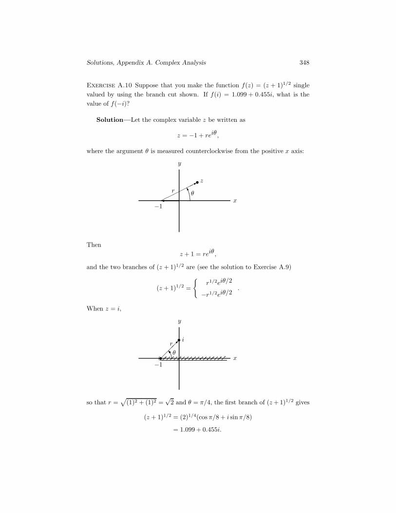
Solutions, Appendix A. Complex Analysis 348
Exercise A.10 Suppose that you make the function f(z) = (z + 1)1/2 singlevalued by using the branch cut shown. If f(i) = 1.099 + 0.455i, what is thevalue of f(−i)?
Solution—Let the complex variable z be written as
z = −1 + reiθ,
where the argument θ is measured counterclockwise from the positive x axis:
x
y
z
r θ
−1��$$$$$$/0
�.....................................................
Thenz + 1 = reiθ,
and the two branches of (z + 1)1/2 are (see the solution to Exercise A.9)
(z + 1)1/2 =
{r1/2eiθ/2
−r1/2eiθ/2.
When z = i,
x
y
r
θ
i
−1����
''���� ........
..........................
so that r =√
(1)2 + (1)2 =√
2 and θ = π/4, the first branch of (z+ 1)1/2 gives
(z + 1)1/2 = (2)1/4(cos π/8 + i sinπ/8)
= 1.099 + 0.455i.

Solutions, Appendix A. Complex Analysis 349
To have a single-valued function, we must remain on the first branch. Whenz = −i,
x
y
r
θ
−i
−1���.��
���� ........
............................
.......................................................................................................................................................................................................
so that r =√
2 and θ = 7π/4, the first branch of (z + 1)1/2 gives
(z + 1)1/2 = (2)1/4(cos 7π/8 + i sin 7π/8)
= −1.099 + 0.455i.
Exercise A.11 Suppose that you make the function f(z) = (z2 + 1)1/2 singlevalued by using the branch cuts shown. If f(1 + 2i) = 1.112 + 1.799i, what isthe value of f(−1 + 2i)?
Solution—Notice that
f(z) = (z − i)1/2(z + i)1/2,
so f(z) is the product of two multivalued functions. We introduce variables r1,r2, θ1, and θ2 defined as shown below:

Solutions, Appendix A. Complex Analysis 350
x
y
r1
r2
θ1
θ2
i
−i
$$$$/
$$$$/
0
0
�
�
� �
� �
........
................
........
................
If the complex variable z is written as
z = i+ r1eiθ1 ,
thenz − i = r1e
iθ1
and the two branches of (z − i)1/2 are (see the solution to Exercise A.9)
(z − i)1/2 =
{r1/21 eiθ1/2
−r1/21 eiθ1/2
.
Then if we write the complex variable z as
z = −i+ r2eiθ2 ,
the expressionz + i = r2e
iθ2
and the two branches of (z + i)1/2 are
(z + i)1/2 =
{r1/22 eiθ2/2
−r1/22 eiθ2/2
.
When z = 1 + 2i,

Solutions, Appendix A. Complex Analysis 351
x
y
r1
r2
θ1
θ2
i
−i
����
���������1
'
2
�
�
�� �
� �
........
....................
........
.....................................
..................
the termsr1 =
√(1)2 + (1)2 =
√2,
r2 =√
(1)2 + (3)2 =√
10,
θ1 = arctan(1/1) = 45◦,
θ2 = arctan(3/1) = 71.6◦.
Using the first branches of the two square roots, we obtain
f(1 + 2i) = r1/21 r
1/22 ei(θ1 + θ2)/2
= 1.112 + 1.799i.
To obtain a single-valued function, we must continue to use the first branchesof the square roots. When z = −1 + 2i,
x
y
r1
r2
θ1
θ2−i
���'
���������3
�
�
�
�
�� �
� �
...........................................................................................
.................................................
........
......................................
.................................................

Solutions, Appendix A. Complex Analysis 352
the termsr1 =
√2,
r2 =√
10,
θ1 = −225◦,
θ2 = 90◦ + arctan(1/3) = 108◦.
Using the first branches of the two square roots, we obtain
f(−1 + 2i) = r1/21 r
1/22 ei(θ1 + θ2)/2
= 1.112− 1.799i.

Appendix A
Complex Analysis
Complex variables are used extensively in the theory of elasticwave propagation. In this appendix we briefly summarize the resultsfrom complex analysis used in this book.
A.1 Complex Variables
Here we define a complex variable, give examples of functions of a complexvariable, and show how complex variables can be represented by points on aplane. We also define the derivative of a function of a complex variable andanalytic functions.
A complex variable is a variable of the form x+ iy, where x and y are realvariables and i is defined to have the property that i2 = −1. The variable x iscalled the real part of z, and the variable y is called the imaginary part. Wedenote the real and imaginary parts of a complex variable by the notations
x = Re(z), y = Im(z).
The magnitude |z| of a complex variable z is defined by
|z| = (x2 + y2)1/2,
and the conjugate z of z is defined by
z = x− iy.
353
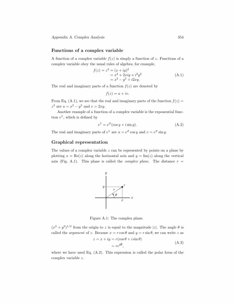
Appendix A. Complex Analysis 354
Functions of a complex variable
A function of a complex variable f(z) is simply a function of z. Functions of acomplex variable obey the usual rules of algebra; for example,
f(z) = z2 = (x+ iy)2
= x2 + 2xiy + i2y2
= x2 − y2 + i2xy.(A.1)
The real and imaginary parts of a function f(z) are denoted by
f(z) = u+ iv.
From Eq. (A.1), we see that the real and imaginary parts of the function f(z) =z2 are u = x2 − y2 and v = 2xy.
Another example of a function of a complex variable is the exponential func-tion ez , which is defined by
ez = ex(cos y + i sin y). (A.2)
The real and imaginary parts of ez are u = ex cos y and v = ex sin y.
Graphical representation
The values of a complex variable z can be represented by points on a plane byplotting x = Re(z) along the horizontal axis and y = Im(z) along the verticalaxis (Fig. A.1). This plane is called the complex plane. The distance r =
x
y
x
y zr
θ4(((((�....................................................................................................................
Figure A.1: The complex plane.
(x2 + y2)1/2 from the origin to z is equal to the magnitude |z|. The angle θ iscalled the argument of z. Because x = r cos θ and y = r sin θ, we can write z as
z = x+ iy = r(cos θ + i sin θ)
= reiθ,(A.3)
where we have used Eq. (A.2). This expression is called the polar form of thecomplex variable z.

Appendix A. Complex Analysis 355
Derivatives and analytic functions
The derivative of a function of a complex variable f(z) is defined in exactly thesame way as the derivative of a function of a real variable:
df(z)dz
= limΔz→0
f(z + Δz) − f(z)Δz
.
By writing f(z) = u(x, y) + iv(x, y) and Δz = Δx+ iΔy, we can express thisdefinition in the form
df(z)dz
= limΔx,Δy→0
∂u
∂xΔx+
∂u
∂yΔy + i
∂v
∂xΔx+ i
∂v
∂yΔy
Δx+ iΔy. (A.4)
Depending upon how Δx and Δy approach zero, the point z+Δz approaches zalong different paths in the complex plane. We set Δx = Δr cos θ and Δy =Δr sin θ, where Δr is the magnitude of Δz and the angle θ is the argumentof Δz (Fig. A.2). Equation (A.4) becomes
x
y
z
z + ΔzΔr
θ4((((��
Δx
Δy
Figure A.2: Points z and z + Δz in the complex plane.
df(z)dz
=
∂u
∂xcos θ +
∂u
∂ysin θ + i
∂v
∂xcos θ+ i
∂v
∂ysin θ
cos θ + i sin θ.
Multiplying this equation by cos θ − i sin θ, we obtain the result
df(z)dz
=(∂v
∂y− i
∂u
∂y
)sin2 θ +
(∂u
∂y+ i
∂v
∂y− i
∂u
∂x+∂v
∂x
)sin θ cos θ
+(∂u
∂x+ i
∂v
∂x
)cos2 θ.
(A.5)This expression is independent of the angle θ (that is, the value of the derivativeof f(z) is independent of the path along which z+Δz approaches z) only if the

Appendix A. Complex Analysis 356
coefficients of sin2 θ and cos2 θ are equal and the coefficient of sin θ cos θ equalszero. This requires that
∂u
∂x=
∂v
∂y,
∂u
∂y= −∂v
∂x.
(A.6)
These two equations, which are necessary conditions for the derivative of f(z)to have a unique value at z, are called the Cauchy-Riemann equations. Whenthey are satisfied, Eq. (A.5) becomes
df(z)dz
=∂u
∂x− i
∂u
∂y=∂v
∂y+ i
∂v
∂x.
If the partial derivatives ∂u/∂x, ∂u/∂y, ∂v/∂x, and ∂v/∂y are continuousand the Cauchy-Riemann equations are satisfied at a point z, the function f(z)is said to be analytic at z. When a function is analytic at every point, we simplysay that it is analytic.
Several important classes of functions are analytic or are analytic almosteverywhere in the complex plane.
• Polynomials of the form
f(z) = a0 + a1z + a2z2 + · · ·+ aNz
N , (A.7)
where a0, a1, a2, . . . , aN are constants, are analytic.
• Rational functions of the form
f(z) =p(z)q(z)
=a0 + a1z + a2z
2 + · · ·+ aNzN
b0 + b1z + b2z2 + · · ·+ bMzM(A.8)
are analytic except at points of the complex plane where q(z) = 0.
• Analytic functions of analytic functions are analytic.
A.2 Contour Integration
We first introduce the concept of contour integration and state the Cauchyintegral theorem. We then define poles and show how to evaluate contour inte-grals around closed contours that contain poles. We also discuss multiple-valuedcomplex functions and describe the use of branch cuts.
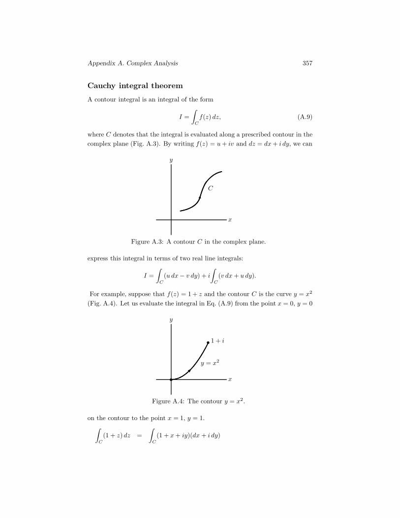
Appendix A. Complex Analysis 357
Cauchy integral theorem
A contour integral is an integral of the form
I =∫
C
f(z) dz, (A.9)
where C denotes that the integral is evaluated along a prescribed contour in thecomplex plane (Fig. A.3). By writing f(z) = u+ iv and dz = dx+ i dy, we can
x
y
C
55
Figure A.3: A contour C in the complex plane.
express this integral in terms of two real line integrals:
I =∫
C
(u dx− v dy) + i
∫C
(v dx+ u dy).
For example, suppose that f(z) = 1 + z and the contour C is the curve y = x2
(Fig. A.4). Let us evaluate the integral in Eq. (A.9) from the point x = 0, y = 0
x
y
1 + i
y = x2
�
�
��
Figure A.4: The contour y = x2.
on the contour to the point x = 1, y = 1.∫C
(1 + z) dz =∫
C
(1 + x+ iy)(dx + i dy)

Appendix A. Complex Analysis 358
=∫
C
[(1 + x) dx− y dy] + i
∫C
[y dx+ (1 + x) dy]
=∫ 1
0
(1 + x) dx−∫ 1
0
y dy + i
∫ 1
0
x2 dx+ i
∫ 1
0
(1 + y1/2) dy
= 1 + 2i.
The Cauchy integral theorem states that if a function f(z) is analytic on andwithin a closed, piecewise smooth contour C,∫
C
f(z) dz = 0.
Poles
If a function f(z) is not analytic at a point z0 of the complex plane, but isanalytic in some neighborhood 0 < |z − z0| < ε, where ε is a positive realnumber, the point z0 is called an isolated singularity of the function f(z). Ifa point z0 is an isolated singularity of f(z), but the limit of f(z) as z → z0
exists and is single valued, the point z0 is called a removable isolated singularityof f(z). When this is the case, the function f(z) is analytic at the point z0 ifthe value of f(z) at z0 is defined to be
f(z0) = limz→z0
f(z).
Let k be a positive integer. If the function (z − z0)kf(z) is analytic orhas a removable isolated singularity at z0, but (z − z0)k−1f(z) has an isolatedsingularity at z0 that is not removable, f(z) is said to have a kth-order poleat z0.
Suppose that we wish to evaluate the contour integral of a function f(z)about a closed contour C, and let us assume that f(z) is analytic on and withinCexcept at a finite number N of poles (Fig. A.5.a). That is, we want to evaluatethe integral
I =∫
C+f(z) dz, (A.10)
where the superscript + indicates that the integral is evaluated in the counter-clockwise direction. We cannot use the Cauchy integral theorem to evaluate thisintegral because the function f(z) is not analytic within the contour. However,we can apply the Cauchy integral theorem to the contour shown in Fig. A.5.b:∫
C+f(z) dz +
N∑k=1
∫C−
k
f(z) dz = 0,

Appendix A. Complex Analysis 359
x
y
C
(a)
1 2
N
��� �����
x
y
C
(b)
C1 C2
CN
��� ����
����
�...........................................................
........................................................................................................
�................................................................................................................................................................�..................................................................................................................................................
..............
x
y
(c)
C1 C2
CN
�����
����
�...........................................................
.................................................................................................................
�....................................................................................................................................................................
........�.................................................................................................................................................................
...........
Figure A.5: (a) A contour C containing a finite number N of poles. (b) A con-tour that doesn’t contain the poles. (c) Circular contours around the individualpoles.

Appendix A. Complex Analysis 360
where C−k is a circular contour about the k th pole. The − superscript indicates
that the integral is evaluated in the clockwise direction. This result shows thatthe integral over the contour C can be expressed as the sum of integrals overclosed circular contours about the poles of f(z) within C (Fig. A.5.c):∫
C+f(z) dz =
N∑k=1
∫C+
k
f(z) dz.
The usefulness of this result derives from the fact that simple expressions canbe derived for the contour integral of a function f(z) about a pole.
Residues
Suppose that a function f(z) has a first-order pole at a point z0. From thedefinition of a first-order pole, this means that the function φ(z) = (z − z0)f(z)has a removable isolated singularity at z0. We make the function φ(z) analyticat z0 by defining
φ(z0) = limz→z0
(z − z0)f(z).
Our objective is to evaluate the integral∫C
f(z) dz =∫
C
φ(z)z − z0
dz (A.11)
for a closed circular contour C of radius R around z0 (Fig. A.6.a). (We choose Rso that the function φ(z) is analytic on and within C.) Let z be a point on the
(a)
x
y
R
z0 C� ...............
..................................................................................................................................................................................................................................................................................................................................................
..........
����
(b)
x
y
z
z0
θ� .................................................................................................................................................................................................................................................................................................................................................................
..........
$$$$$$/
�����
����,
Figure A.6: (a) Circular contour around a pole z0. (b) A point z on the contour.
contour C. We can express z − z0 in polar form as (Fig. A.6.b)
z − z0 = Reiθ.

Appendix A. Complex Analysis 361
Using this expression, we can write Eq. (A.11) as∫C
f(z) dz =∫ 2π
0
iφ(z0 +Reiθ) dθ. (A.12)
To evaluate the integral on the right side, we express the function φ(z0 +Reiθ)in a Taylor series:
φ(z0 +Reiθ) = φ(z0) +dφ
dz(z0)Reiθ + 1
2
d2φ
dz2(z0)R2ei2θ + · · ·
= φ(z0) +∞∑
n=0
1n!dnφ
dzn(z0)Rneinθ.
We substitute this result into Eq. (A.12), obtaining the equation∫C
f(z) dz = iφ(z0)∫ 2π
0
dθ+∞∑
n=1
i
n!dnφ
dzn(z0)Rn
∫ 2π
0
einθ dθ.
The integrals ∫ 2π
0
einθ dθ = 0
for n = 1, 2, . . . Therefore we obtain the result∫C
f(z) dz = 2πiφ(z0) = 2πi limz→z0
(z − z0)f(z).
This equation gives the value of the contour integral of a function f(z) whenthe function is analytic on and within the contour except at a first-order pole z0within the contour. This result can be extended to the case when f(z) is analyticon and within the contour except at a kth-order pole z0:∫
C
f(z) dz = 2πi1
(k − 1)!lim
z→z0
dk−1
dzk−1[(z − z0)kf(z)].
The term1
(k − 1)!lim
z→z0
dk−1
dzk−1[(z − z0)kf(z)] (A.13)
is called the residue of a kth-order pole. Using this terminology, we can writethe value of the contour integral of a function f(z) that is analytic on and withinthe contour except at a finite number of poles in the simple form∫
C
f(z) dz = 2πi∑
Residues.
As an example, we evaluate the integral∫C
f(z) dz =∫
C
2z2
z2 − 2z − 3dz

Appendix A. Complex Analysis 362
x
y
2C
........
........
.............................................
........................
..................................................................................................................................................................................................................................................................................................................................................................................
..................................................................................�
��' '
Figure A.7: A closed contour C.
for the closed contour C shown in Fig. A.7. The integrand is a rational function(see Eq. (A.8)) and is analytic except at points where the denominator equalszero. It can be written
f(z) =2z2
(z + 1)(z − 3).
This function has first-order poles at z = −1 and at z = 3. The pole at z = 3is not within the contour. The residue of the pole at z = −1 is
Residue = limz→−1
(z + 1)2z2
(z + 1)(z − 3)= −1
2 .
The value of the integral is 2πi(−12) = −πi.
Exercises
Exercise A.1 Show that the magnitude of a complex variable z is given bythe relation
|z| = (zz)1/2.
Exercise A.2 Show that for any two complex numbers z1 and z2,
|z1z2| = |z1||z2| and∣∣∣∣z1z2
∣∣∣∣ =|z1||z2|
.
Discussion—Express z1 and z2 in polar form.
Exercise A.3
(a) Show that the exponential function f(z) = ez is analytic.(b) Show that the function f(z) = z is not analytic anywhere.

Appendix A. Complex Analysis 363
Exercise A.4
x
y
1 + i
�
�
��
��
Evaluate the contour integral ∫C
(1 + z) dz
along the contour shown from the point z = 0 to the point z = 1 + i. Compareyour result with the result of the example on page 357.
Exercise A.5
(a) Show that the function
f(z) =1
z − 1has a first-order pole at z = 1.(b) Show that the function
f(z) =1
(z − 1)2
has a second-order pole at z = 1.
Exercise A.6
x
y
2C
........
........
............................................
.......................
.......................................................................................................................................................................................... �
��' '
�
Evaluate the contour integral ∫C
dz
z2 + 1for the closed contour shown.
Discussion—Find the poles of the integrand by locating the points wherez2 + 1 = 0.
Answer: The value of the integral is π.

Appendix A. Complex Analysis 364
Exercise A.7
x
y
2C
........
........
............................................
........................
...................................................................................................................................................................................................................................................................................................................................................................................
..................................................................................�
��' '
Evaluate the contour integral ∫C
dz
z(z − 1)(z − 3)2
for the closed circular contour shown.Answer: The value of the integral is 5
18πi.

Appendix A. Complex Analysis 365
A.3 Multiple-Valued Functions
Some functions f(z) can have more than one value for a given value of z. Inthis section we describe the most common multiple-valued functions and showhow branch cuts are used to insure that they remain single valued.
Examples
Only three types of multiple-valued functions occur commonly in complex anal-ysis: roots, logarithms, and complex variables with complex exponents.
Roots
The square root of the complex variable z is defined by the expression
z1/2 = (reiθ)1/2 = r1/2eiθ/2. (A.14)
That is, the square root of z is defined in terms of its magnitude r and itsargument θ, and we see that(
r1/2eiθ/2)(
r1/2eiθ/2)
= reiθ = z.
If we increase the argument by 2π, the magnitude r and the argument θ + 2πdefine the same point z in the complex plane. However, this magnitude andargument give us a different value of the square root of z:
z1/2 = [rei(θ + 2π)]1/2 = r1/2ei(θ + 2π)/2.
It is easy to confirm that this square root is equal to the negative of the squareroot in Eq. (A.14):
r1/2ei(θ + 2π)/2 = −r1/2eiθ/2,
which is analogous to the square root of a real number.A natural question is whether there are more values of the square root of z.
Although the magnitude r and the argument θ + 2πn, where n is any integer,also define the same point z in the complex plane, it is easy to confirm thatthere are only two values of the square root of z. In fact, the complex variable zraised to the 1/n power has exactly n roots:
z1/n = r1/nei(θ + 2πm)/n, m = 0, 1, · · · , n− 1. (A.15)
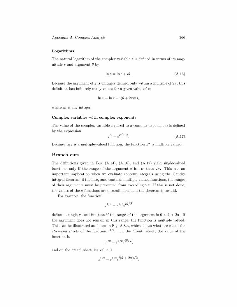
Appendix A. Complex Analysis 366
Logarithms
The natural logarithm of the complex variable z is defined in terms of its mag-nitude r and argument θ by
ln z = ln r + iθ. (A.16)
Because the argument of z is uniquely defined only within a multiple of 2π, thisdefinition has infinitely many values for a given value of z:
ln z = ln r + i(θ + 2πm),
where m is any integer.
Complex variables with complex exponents
The value of the complex variable z raised to a complex exponent α is definedby the expression
zα = eα ln z. (A.17)
Because ln z is a multiple-valued function, the function zα is multiple valued.
Branch cuts
The definitions given in Eqs. (A.14), (A.16), and (A.17) yield single-valuedfunctions only if the range of the argument θ is less than 2π. This has animportant implication when we evaluate contour integrals using the Cauchyintegral theorem; if the integrand contains multiple-valued functions, the rangesof their arguments must be prevented from exceeding 2π. If this is not done,the values of these functions are discontinuous and the theorem is invalid.
For example, the function
z1/2 = r1/2eiθ/2
defines a single-valued function if the range of the argument is 0 < θ < 2π. Ifthe argument does not remain in this range, the function is multiple valued.This can be illustrated as shown in Fig. A.8.a, which shows what are called theRiemann sheets of the function z1/2. On the “front” sheet, the value of thefunction is
z1/2 = r1/2eiθ/2,
and on the “rear” sheet, its value is
z1/2 = r1/2ei(θ + 2π)/2.

Appendix A. Complex Analysis 367
(a)
x
y
z
������
� �
(b)
x
y
Branch point Branch cut��� ��'
���
Figure A.8: (a) The Riemann sheets of the function f(z) = z1/2. (b) A branchcut in the complex plane.
In the figure we show an integration path in the complex plane that goes froma point z with argument π/4 to the same point z with argument π/4 + 2π.Observe that the function is multiple valued at z. As a consequence, its valueon the integration path is discontinuous.
Multiple-valued functions are avoided by using what are called branch cutsin the complex plane. A branch cut is simply a line in the complex plane thatintegration paths are not permitted to cross. This line is said to be “cut” fromthe complex plane. Figure A.8.b shows a branch cut along the positive real axis.On any integration path that does not cross this branch cut, the argument of zremains in the range 0 < θ < 2π and the function z1/2 is single valued. Theendpoint of a branch cut is called a branch point. Notice that any continuousline that begins at z = 0 and extends to infinity is an acceptable branch cut tomake the function z1/2 single valued.
As a second example, consider the function
f(z) = (z − z0)1/2.
By writing z as z = z0 + reiθ (Fig. A.9.a), we can see that f(z) has the twovalues
f(z) =
{r1/2eiθ/2,
r1/2ei(θ + 2π)/2.
We can make this function single valued by introducing the branch cut shownin Fig. A.9.b. It insures that θ remains in the range −3π/2 < θ < π/2. Observe

Appendix A. Complex Analysis 368
(a)
x
y
rz
z0
θ&�������
�6
(b)
x
y
z0
Branchpoint
Branchcut�����7
����� �
Figure A.9: (a) The points z0 and z. (b) A branch cut in the complex plane.
that the branch point is the point at which the expression within the squareroot equals zero.
Exercises
Exercise A.8 By using the definition of the square root of the complex vari-able z given in Eq. (A.15), show that:(a) the two values of the square root of 1 are +1 and −1;(b) the two values of the square root of i are 1
2
√2(1 + i) and −1
2
√2(1 + i).
Exercise A.9 By using the definition of the square root of the complex vari-able z given in Eq. (A.15), show that there are only two values of the squareroot of z.
Exercise A.10 Suppose that you make the function f(z) = (z + 1)1/2 singlevalued by using the branch cut
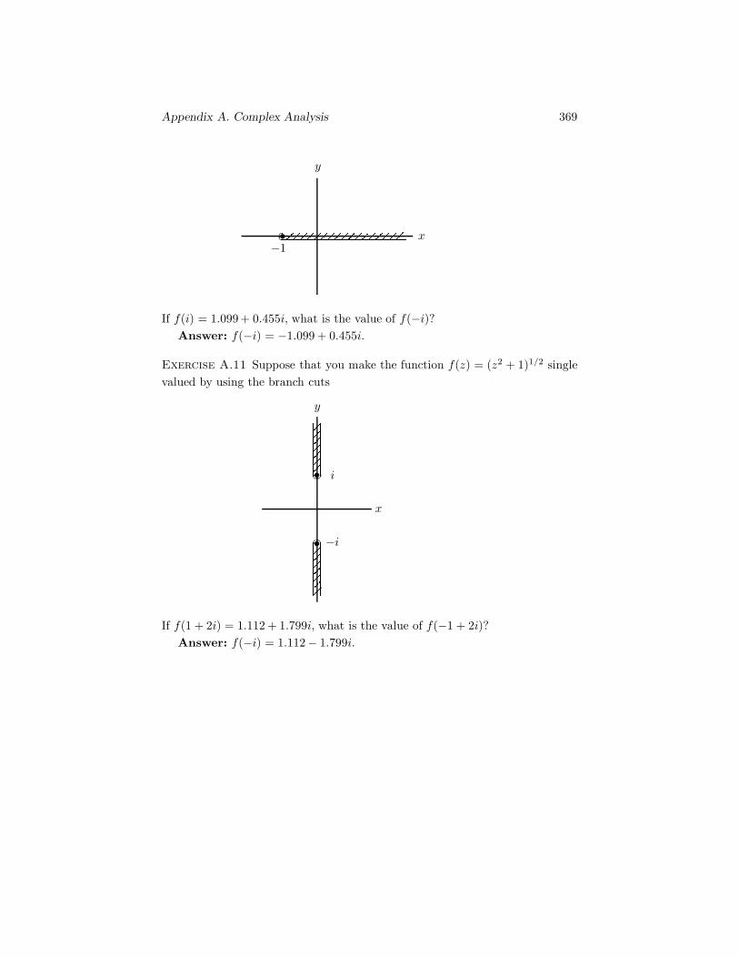
Appendix A. Complex Analysis 369
x
y
−1���
If f(i) = 1.099 + 0.455i, what is the value of f(−i)?Answer: f(−i) = −1.099 + 0.455i.
Exercise A.11 Suppose that you make the function f(z) = (z2 + 1)1/2 singlevalued by using the branch cuts
x
y
i
−i
�
�
� �
� �
If f(1 + 2i) = 1.112 + 1.799i, what is the value of f(−1 + 2i)?Answer: f(−i) = 1.112− 1.799i.
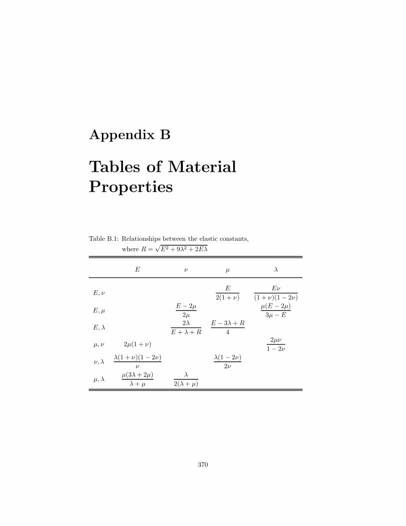
Appendix B
Tables of MaterialProperties
Table B.1: Relationships between the elastic constants,
where R =√E2 + 9λ2 + 2Eλ
E ν μ λ
E, νE
2(1 + ν)Eν
(1 + ν)(1 − 2ν)
E, μE − 2μ
2μμ(E − 2μ)
3μ− E
E, λ2λ
E + λ+ R
E − 3λ+ R
4
μ, ν 2μ(1 + ν)2μν
1 − 2ν
ν, λλ(1 + ν)(1 − 2ν)
ν
λ(1 − 2ν)2ν
μ, λμ(3λ+ 2μ)λ+ μ
λ
2(λ+ μ)
370

Appendix B. Tables of Material Properties 371
Table B.2: Properties of various solids
Material ρ α β E ν λ μ
(Mg/m3) (km/s) (km/s) (GPa) (GPa) (GPa)
Aluminum (rolled) 2.70 6.42 3.04 67.6 0.35 61.3 24.9Beryllium 1.87 12.8 8.88 309 0.04 15.7 147Bismuth 9.80 2.20 1.10 31.6 0.33 23.7 11.8Brass (yellow) 8.64 4.70 2.10 104 0.37 114 38.1Cadmium 8.60 2.80 1.50 50.2 0.29 28.7 19.3Copper (rolled) 8.93 5.01 2.27 126 0.37 132 46.0Epon 828 1.21 2.83 1.23 5.06 0.38 6.02 1.83Fused silica 2.20 5.70 3.75 69.2 0.11 9.60 30.9Glass (pyrex) 2.24 5.64 3.28 59.9 0.24 23.0 24.0Gold (hard drawn) 19.7 3.24 1.20 80.5 0.42 150 28.3Ice 0.91 3.99 1.98 9.61 0.33 7.40 3.59Iron 7.69 5.90 3.20 203 0.29 110 78.7Iron (cast) 7.22 4.60 2.60 123 0.26 55.1 48.8Lead 11.2 2.20 0.70 15.8 0.44 43.2 5.48Magnesium 1.73 5.80 3.00 41.2 0.31 27.1 15.6Molybdenum 10.0 6.30 3.40 299 0.29 165 115Nickel 8.84 5.60 3.00 206 0.29 118 79.5Platinum 21.4 3.26 1.73 167 0.30 99.3 64.0Silver 10.6 3.60 1.60 74.7 0.37 83.1 27.1Steel (mild) 7.80 5.90 3.20 206 0.29 111 79.8Steel (stainless) 7.89 5.79 3.10 196 0.29 112 75.8Titanium carbide 5.15 8.27 5.16 323 0.18 77.9 137Tungsten 19.4 5.20 2.90 415 0.27 198 163Zircaloy 9.36 4.72 2.36 139 0.33 104 52.1Nylon (6/6) 1.12 2.60 1.10 3.77 0.39 4.86 1.35Polyethylene 0.90 1.95 0.54 0.76 0.45 2.89 0.26Polystyrene 1.05 2.40 1.15 3.75 0.35 3.27 1.38

Appendix B. Tables of Material Properties 372
Table B.3: Properties of various liquids
Material ρ α λ
(Mg/m3) (km/s) (GPa)
Acetonyl acetone 0.72 1.40 1.42Alcohol (ethanol 25◦C) 0.79 1.20 1.15Alcohol (methanol) 0.79 1.10 0.96Argon (87K) 1.43 0.84 1.00Carbon tetrachloride (25◦C) 1.59 0.92 1.36Chloroform (25◦C) 1.49 0.98 1.45Fluorinert (FC-40) 1.86 0.64 0.76Gasoline 0.80 1.25 1.25Glycol (polyethylene 200) 1.08 1.62 2.85Helium-4 (2K) 0.14 0.22 0.00Honey (Sue Bee orange) 1.42 2.03 5.85Kerosene 0.81 1.32 1.41Nitromethane 1.13 1.33 1.99Oil (baby) 0.82 1.43 1.67Oil (jojoba) 1.17 1.45 2.47Oil (olive) 0.91 1.44 1.91Oil (peanut) 0.91 1.43 1.88Oil (SAE 30) 0.87 1.70 2.51Oil (sperm) 0.88 1.44 1.82Turpentine (25◦C) 0.88 1.25 1.38Water (20◦C) 1.10 1.40 2.16

Appendix B. Tables of Material Properties 373
Table B.4: Properties of various gases
Material ρ α λ
(kg/m3) (km/s) (MPa)
Air (dry at 0◦C) 1.29 0.33 0.14Carbon dioxide (0◦C) 1.97 0.25 0.13Helium (0◦C) 0.17 0.96 0.16Nitrogen (0◦C) 1.25 0.33 0.13Oxygen (0◦C) 1.42 0.31 0.14Oxygen (20◦C) 1.32 0.32 0.14


