Introduction toIntroduction toDynamical SystemsDynamical Systems

A HANDS-ON APPROACH WITH MAXIMA

Jaime E. Villate9 789729 939600

ISBN 972-99396-0-8

Introduction to Dynamical Systems

A Hands-on Approach with Maxima

Jaime E. VillateUniversity of Porto

College of EngineeringPorto, Portugal

Introduction to dynamical systems: a hands-on approach with MaximaCopyright c© 2006 Jaime E. VillateE-mail: villate@fe.up.pt

This work is licensed under the Creative Commons Attribution-Share Alike 2.5 License. To view a copy ofthis license, visit http://creativecommons.org/licenses/by-sa/2.5/ or send a letter to CreativeCommons, 543 Howard Street, 5th Floor, San Francisco, California, 94105, USA.

ISBN: 972-99396-0-8

This is a partial translation of Portuguese version 1.2 of February 27, 2007.

The cover figure is the Julia set for the complex number −0.75+ i0.1, with 48 iterations, as explained inchapter 12.

Contents

Preface vii

1 Introduction 11.1 Differential equations . . . . . . . . . . . . . . . . . . . . . . . . . . . . . . . . 1

1.2 Solving physics problems with Maxima . . . . . . . . . . . . . . . . . . . . . . 1

1.3 References . . . . . . . . . . . . . . . . . . . . . . . . . . . . . . . . . . . . . . 7

1.4 Multiple-choice questions . . . . . . . . . . . . . . . . . . . . . . . . . . . . . . 7

1.5 Problems . . . . . . . . . . . . . . . . . . . . . . . . . . . . . . . . . . . . . . 8

2 Discrete dynamical systems 92.1 Discrete systems evolution . . . . . . . . . . . . . . . . . . . . . . . . . . . . . 12

2.2 Graphical analysis . . . . . . . . . . . . . . . . . . . . . . . . . . . . . . . . . . 12

2.3 Fixed points . . . . . . . . . . . . . . . . . . . . . . . . . . . . . . . . . . . . . 15

2.4 Periodic points . . . . . . . . . . . . . . . . . . . . . . . . . . . . . . . . . . . 17

2.5 Solving equations numerically . . . . . . . . . . . . . . . . . . . . . . . . . . . 19

2.5.1 Iteration method . . . . . . . . . . . . . . . . . . . . . . . . . . . . . . 19

2.5.2 Newton’s method . . . . . . . . . . . . . . . . . . . . . . . . . . . . . . 21

2.6 References . . . . . . . . . . . . . . . . . . . . . . . . . . . . . . . . . . . . . . 23

2.7 Multiple-choice questions . . . . . . . . . . . . . . . . . . . . . . . . . . . . . . 23

2.8 Problems . . . . . . . . . . . . . . . . . . . . . . . . . . . . . . . . . . . . . . 24

Index 26

Bibliography 27

iv CONTENTS

List of Figures

1.1 Power dissipated in a resistor . . . . . . . . . . . . . . . . . . . . . . . . . . . . 4

1.2 Trajectory of a particle . . . . . . . . . . . . . . . . . . . . . . . . . . . . . . . 7

2.1 Evolution of yn+1 = cos(yn) with y0 = 2. . . . . . . . . . . . . . . . . . . . . . . 13

2.2 Staircase diagram for xn+1 = cos(xn) with x0 = 2. . . . . . . . . . . . . . . . . . 13

2.3 Solutions of the system yn+1 = y2n−0.2. . . . . . . . . . . . . . . . . . . . . . . 14

2.4 Solutions of the discrete logistic model . . . . . . . . . . . . . . . . . . . . . . . 15

2.5 Newton’s method for finding roots of an equation. . . . . . . . . . . . . . . . . . 22

vi LIST OF FIGURES

Preface

This book is updated very often. The number of the current version can be found on the secondpage and the most recent version can always be found on the Web at http://fisica.fe.up.pt/maxima/dynamicalsystems. This version has been written to be used with Maxima’s version5.11. (http://maxima.sourceforge.net).

This book started as the lecture notes for a one-semester course on the physics of dynamicalsystems, taught at the College of Engineering of the University of Porto, since 2003. The subjectof this course on dynamical systems is at the borderline of physics, mathematics and computing,and it substituted a course on classical mechanics that we used to teach to students majoring incomputing engineering.

Since dynamical systems is usually not taught with the traditional axiomatic method used in otherphysics and mathematics courses, but rather with an empiric approach, it is more appropriate touse a practical teaching method based on projects done with a computer.

The study of dynamical systems advanced very quickly in the decades of 1960 and 1970, givingrise to a whole new area of research with an innovative methodology that gave rise to heated de-bates within the scientific community. The innovative boost was fueled by the rapid developmentof computers.

A new generation of researchers rose, who used their computers as laboratories for experimentingwith equations discovering new phenomena. The traditional mathematicians criticized that ap-proach for the lack of a rigorous mathematical foundations for those new results. Many of thoseresults were found within the framework of physical problems: non-linear dynamics, condensed-matter physics and electromagnetism. However, many physicists regarded that new research fieldsimply as a computer simulation of old physical concepts long established, without any newphysics in it. A usual comment would be: “this is all very nice, but where is the physics init?”.

Thus, the pioneers in this new field of dynamical systems would be often confronted with rejectedpublications in scientific journals and negative assessments of their work. On the other hand, theiractivities awakened a strong interest that increased very quickly and were viewed by some as arefreshing new trend; the methods used in the study of dynamical systems match well with theworking environment of modern scientists.

The new paradigm spread to teaching and the traditional courses on physics and mathematicshave been gradually “infected” with this new experimental/ computational methodology, contrast-ing with the traditional axiomatic method. As it happened in the scientific community, the newmethodology has also led to some debate among teachers; at the same time, it has awakened biginterest as a better way to motivate today’s students. Subjects such as chaos and fractals are very

viii Preface

appealing to them.

In this book we intend to explore some topics on dynamical systems, using an active teachingapproach, supported by computing tools and trying to avoid too may abstract details. The use of aComputer Algebra System (CAS) does not eliminate the need for mathematical analysis from thestudent; using a CAS to teach an engineering course does not turn it into a purely technical subjecteither. One of the difficulties inherent to any Computer Algebra System is the fact that there areno unique solutions to the problems it solves. Different methods to solve a problem may lead tosolutions that look very different but might be equivalent. Or the solutions can be really differentand only equivalent within some domain. In some cases the system does not give any answer or itmight even give a wrong answer.

It is necessary to gain some experience to be able to use CAS tools successfully and to be able totest the validity of its results. In the process of gaining that experience, the user will also gain abetter insight into the mathematical methods implemented in the system.

Nowadays the great majority of engineering and exact sciences professionals depend on a calcu-lator to calculate the square root of a real number, for instance, 3456. Some of us were taught inSchool how to do that with pencil an paper, in a time when there were no calculators. I do notbelieve that this new dependency is a serious handicap, and I’m not in favor of teaching kids howto calculate square roots with paper and pencil before they are allowed to use the calculator. WhatI find very important is that the algorithm we used to calculate square roots with paper and pencilremains available and well documented in the literature; it is an valuable piece in our legacy ofalgorithms.

On the other hand, now that students have calculators to compute square roots, they can movefaster into other topics such as the study of quadratic equations; and in doing so, they might evengain a deeper insight of the function

√x, which they did not attain when they had to spend a

lot of time learning the algorithm to calculate square roots. In the case of differential equationsand difference equations, with the help of Computer Algebra Systems students can advance fasterinto subjects such as chaos and fractals, instead of dedicating a whole semester to learn severalalgorithms to obtain analytical solutions for a few types of equations.

I would like to acknowledge the help of my colleagues Helena Braga and Francisco Salzedas, withwhom I have taught the course on Physics of Dynamical Systems; I would also like to thank ourstudents in that course throughout the last 3 years; their positive comments have encouraged meto undertake the task of writing this book. The students have been asked to make projects forthat course, and some of those projects were very interesting and helped me learn some of thesubjects covered in this book. Special thanks go to the student Pedro Martins and to my colleagueFrancisco Salzedas, who made a careful review of the manuscript.

Jaime E. VillatePorto, February 2007

Chapter 1

Introduction

1.1 Differential equations

Differential equations play a very important role in Engineering and Science. Many problems leadto one or several differential equations that must be solved. Most attention has been given to linearequations in the literature; several analytical methods have been developed to solve that type ofequations.

Non-linear differential equations are much harder to analyze and there are no general solutiontechniques for those equations. Problems that lead to linear equations are easier to study. Fromthe last half of the 20th century, the rapid development of the computer made it possible to solvenon-linear problems using numerical methods. Non-linear systems lead to a wealth of new andinteresting phenomena not present in linear systems.

A new approach, that relies more on geometric interpretation rather than analytical analysis, hasgained popularity for the study of non-linear systems. Many of the concepts used in that geomet-rical approach, such as the phase space, have long be used in dynamics to study the motion of amechanical system.

In order to give a short introduction to that methodology to study differential equations, in thenext chapters we will consider several problems specific dynamics and electrical circuit theory.Before we begin, we will introduce a Computer Algebra System (CAS), Maxima, which will beused extensively throughout the book.

1.2 Solving physics problems with Maxima

Maxima is a software package in the category of Computer Algebra Systems (CAS), namely, asystem that can be used not just for numerical calculation but also to deal with algebraic equa-tions with abstract variables. There are various CAS packages available; we have decided to useMaxima because it is Free Software. That means that it can be installed and used by our studentswithout having to obtain a license for it, and they can even study its source code to get a betterunderstanding of how that system works. Another important advantage is the possibility of mod-ifying the original package to better suit our needs; we took advantage of that facility to add new

2 Introduction

features needed for this book.

Maxima includes several functions to manipulate mathematical functions, including differentia-tion, integration, power series approximation, Laplace transforms, solving ordinary differentialequations and graph plotting in 2 and 3 dimensions. It can also work with matrices and vec-tors. Maxima can be used to solve problems numerically and write down programs as done withtraditional programming languages.

The following examples should serve to give a first glimpse at the way Maxima can be used. Inthe next chapters we will go deeper into the subject, but readers who are not familiar with Maximaand would like to have a general overview from the beginning can start by going through appendixA. The examples that we will solve in this section are in the area of dynamics of a particle anddirect-current circuits, which are the main subjects in this book. A minimum knowledge in thosetwo subjects will be necessary in order to follow those examples.

Example 1.1A battery is connected to an external resistor with resistance R and the voltage across the resistoris measured with a voltmeter V. To find the electro-motive force ε and the internal resistance r ofthe battery, two external resistors of 1.13 kΩ and 17.4 kΩ were used. The voltage drop in bothcases were 6.26 V e 6.28 V. Find the intensity of the current in both cases. Obtain the values of ε

and r. Plot a graph of the power dissipated in the external resistance, as a function of R, for valuesof R within 0 and 5r.

Rε, r V

Solution: The current through R is found from Ohm’s law:

I =∆VR

(1.1)

With the values given for the potential difference, ∆V , and the resistance, R, we can use Maximato find the currents:

(%i1) 6.26/1.13e3;(%o1) .005539823008849558

When Maxima’s console is started, the (%i1) label appears indicating that the system is readyto accept a command; the letter “i” stands for input. The expression 1.13e3 is the form used torepresent the number 1.13×103 in Maxima. Each command must end with a semi-colon. Whenthe “Enter” key is pressed, the system responds with a label (%o1) followed by the result of thefirst command (%i1); “o” stands for output.

The current in the second case is computed in a similar way:

1.2 Solving physics problems with Maxima 3

(%i2) 6.28/17.4e3;(%o2) 3.609195402298851E-4

Thus, the current in the 1.13 kΩ resistor is 5.54 mA, and in the 17.4 kΩ resistor is 0.361 mA.

To obtain the battery’s electro-motive force and internal resistance we should use the voltage-current characteristic for a battery:

∆V = ε− rI (1.2)

replacing the two set of values given for ∆V and R we will get a system of two equations with twovariables. We will save those two equations in two Maxima variables that we will dub as eq1 andeq2

(%i3) eq1: 6.26 = emf - r*%o1;(%o3) 6.26 = emf - .005539823008849558 r(%i4) eq2: 6.28 = emf - r*%o2;(%o4) 6.28 = emf - 3.609195402298851E-4 r

notice that the symbol used to save a value in a variable is a colon and not an equal sign. A maximavariable can store a numerical value or something more abstract as a mathematical equation in thiscase. The equal sign makes part of the equation that is being stored. To avoid having to write thenumerical values of the currents obtained previously, we used the symbols %o1 and %o2 that standfor the value of those previous results.

The last two equations constitute a linear system of equations with two variables. That kind ofsystem can be solved in Maxima, using the command solve:

(%i5) solve([eq1,eq2]);983100 79952407

(%o5) [[r = ------, emf = --------]]254569 12728450

(%i6) %,numer;(%o6) [[r = 3.861821352953423, emf = 6.281393806787158]]

The syntax [eq1,eq2] was used to create a list with two elements, which is what the commandsolve expects when there are more than one equation to be solved. Some warning messagesgiven by Maxima were omitted above. The command solve gives an exact result, in the formof two rational numbers. The command in %i6 was used to approximate those rational numberswith fixed-point numbers. The symbol % stands for the output of the last command executed; inthis case it is equivalent to %o5. We thus conclude that the electro-motive force is approximately6.2814 V and the internal resistance is 3.8618 Ω.

The electric power dissipated in the resistance R is

P = RI2

the current I across the external resistor can be calculated in terms of the electro-motive force andthe resistances r and R

I =ε

R+ r

4 Introduction

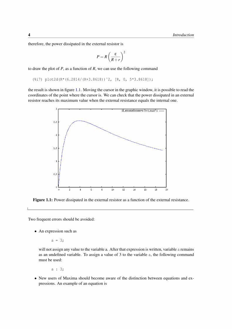
therefore, the power dissipated in the external resistor is

P = R(

ε

R+ r

)2

to draw the plot of P, as a function of R, we can use the following command

(%i7) plot2d(R*(6.2814/(R+3.8618))ˆ2, [R, 0, 5*3.8618]);

the result is shown in figure 1.1. Moving the cursor in the graphic window, it is possible to read thecoordinates of the point where the cursor is. We can check that the power dissipated in an externalresistor reaches its maximum value when the external resistance equals the internal one.

Figure 1.1: Power dissipated in the external resistor as a function of the external resistance.

Two frequent errors should be avoided:

• An expression such as

a = 3;

will not assign any value to the variable a. After that expression is written, variable a remainsas an undefined variable. To assign a value of 3 to the variable a, the following commandmust be used:

a : 3;

• New users of Maxima should become aware of the distinction between equations and ex-pressions. An example of an equation is

1.2 Solving physics problems with Maxima 5

xˆ2 - 3*x = 2*x + 5

while an expression is something like

2*x + 5

Some commands in Maxima accept only equations or expressions as their input values. Forinstance, the command plot2d used in the previous example accepts only expressions andnot equations. The command solve requires one equation, or a list with several equations,but it will also accept expressions instead of equations: each expression given will be auto-matically converted into an equation by equating it to zero; for instance, the command

solve(xˆ2 - 5*x + 5);

will find the two values of x that will solve the equation

x2−5∗ x+5 = 0

Example 1.2The position vector of a particle, as a function of time t, is given by the equation:

~r =(

5− t2 e−t/5)~ex +

(3− e−t/12

)~ey

in MKS units. Find the vectors for the position, velocity and acceleration at t = 0, t = 15 s, andwhen time approaches infinity. Plot the trajectory of the particle during the first 60 seconds of itsmotion.

Solution: We start by representing the position vector as a list with two elements; the first elementwill be the x coordinate and the second one will be the y coordinate. We will save that list in avariable named r, so we can use it later on.

(%i8) r: [5-tˆ2*exp(-t/5),3-exp(-t/12)];2 - t/5 - t/12

(%o8) [5 - t %e , 3 - %e ]

the vector velocity equals the derivative of the position vector and the vector acceleration is thederivative of the vector velocity. The command used in Maxima to find the derivative of an ex-pression is diff. The input to that command can also be a list with several expressions; thus, thevelocity and acceleration are:

(%i9) v: diff(r,t);2 - t/5 - t/12t %e - t/5 %e

(%o9) [---------- - 2 t %e , --------]5 12

(%i10) a: diff(v,t);

6 Introduction

2 - t/5 - t/5 - t/12t %e 4 t %e - t/5 %e

(%o10) [- ---------- + ----------- - 2 %e , - --------]25 5 144

the constant %e in Maxima represents the Euler number, e. To find the position, velocity andacceleration at t = 0, we use the following commands

(%i11) r, t=0, numer;(%o11) [5, 2](%i12) v, t=0, numer;(%o12) [0, .08333333333333333](%i13) a, t=0, numer;(%o13) [- 2, - .006944444444444444]

The argument numer, was used to get the result in floating-point form. In vector notation, theresults we obtained are:

~r(0) = 5~ex+2~ey

~v(0) = 0.08333~ey

~a(0) = −2~ex−0.006944~ey

For t = 15 s the results are obtained in a similar way

(%i14) r, t=15, numer;(%o14) [- 6.202090382769388, 2.71349520313981](%i15) v, t=15, numer;(%o15) [.7468060255179592, .02387539973834917](%i16) a, t=15, numer;(%o16) [0.0497870683678639, - .001989616644862431]

The limiting values when times goes to infinity can be calculated with Maxima’s command limit;the symbol used in Maxima to represent infinity is inf

(%i17) limit(r,t,inf);(%o17) [5, 3](%i18) limit(v,t,inf);(%o18) [0, 0](%i19) limit(a,t,inf);(%o19) [0, 0]

Thus, a particle will approach the point 5~ex +3~ey, where it will remain at rest.

To plot the graph of the trajectory we will use the option parametric of the command plot2d.the x and y components of the position vector will be given separately; the command plot2d willnot accept them inside a list as we have been using them. To get the first element of the list r (xcomponent) is labelled as r[1] and the second element r[2].

1.3 References 7

(%i20) plot2d([parametric,r[1],r[2],[t,0,60],[nticks,100]]);

The time domain, from 0 to 60, is defined with the notation [t,0,60]. The option nticks wasused to increase the number of intervals of t, because the default value of 10 intervals would rendera broken curve instead of a continuous trajectory. The graph obtained is shown in figure 1.2.

Figure 1.2: Trajectory of the particle during the first 60 seconds, from the initial instant when twas equal to 5.2 .

1.3 References

For more information about Maxima, see appendix A and the Maxima Book (de Souza et al.,2003).

1.4 Multiple-choice questions

1. Only one of the following Maxima com-mands is correct. Which one?

A. solve(t-6=0,u-2=0,[t,u]);

B. solve(t+4=0,u-4=0,t,u);

C. solve([xˆ3+4=2,y-4],x,y);

D. solve(x-6=0,y-2=0,[x,y]);

E. solve([t+3,u-4],[t,u]);

2. Newton’s second law was defined in Maximawith:(%i6) F = ma;

which Maxima command should be used tocompute the value of the force correspond-ing to a mass of 7 with an acceleration of 5(SI units).

A. solve(F, m=7, a=5);

8 Introduction

B. solve(F, [m=7, a=5]);

C. solve(%o6, m=7, a=5);

D. %o6, m=7, a=5;

E. solve(F: m=7, a=5)

3. If we input the following commands in Max-ima:

(%i1) x:3$

(%i2) x=5$(%i3) x;

which will be the output (%o3)?

A. 5B. xC. 3

D. true

E. 0

1.5 Problems

1. An ammeter was used to measure the current at points D and F in the circuit which diagramis shown in the figure. At point D the value obtained for the current was 0.944 mA, in thedirection ADC, and at point F it was 0.438 mA, in the direction CFE. (a) Store the equationfor Ohm’s law, V = IR, in a Maxima’s variable “ohm”. (b) Give a value to variable I equal tothe current at point D, and substitute the resistance in Ohm’s law with each of the values 2.2kΩ and 6.8 kΩ, to compute the potential difference in each of the resistors; repeat the sameprocedure to calculate the potential difference in each resistor.

A 6.8 kΩ B 3.3 kΩ E

9 V

F4.7 kΩC

6 V

1.0 kΩ

2.2 kΩD

3 V

2. The position of a particle moving along the x axis is given by the equation x = 2.5 t3−62 t2 +10.3 t, where x is measured in meters and t in seconds. (a) Find the expressions for the velocityand the acceleration as a function of time. (b) Find the values of the time, position and acceler-ation in all the instants when the particle is at rest (v = 0). (c) Draw the plots for the position,velocity and acceleration as a function of time, for t in the interval between 0 and 20 seconds.

3. The position vector of a particle, as a function of time, is given by the equation:

~r =(

5.76− e−t/2.51)~ex + e−t/2.51 cos(3.4 t)~ey

in SI units. (a) Compute the position, velocity and acceleration in the instants t=0, t=8 s, andwhen time goes to infinity. (b) Plot the graphs of the x and y components of the position, asa function of time, for t in the interval between 0 and 15 seconds. (c) Plot the graph of thetrajectory, on the plane xy, in the interval of t between 0 and 15 s.

Chapter 2

Discrete dynamical systems

A discrete dynamical system is a system with a state that only changes at a discrete sequence ofinstants t0, t1, t2, . . .. In the interval between two of those instants the state remains constant.

In this chapter we will only consider first-order discrete systems. In the following chapters themethods used in this chapter will be extended to the case of continuous dynamical systems. In thelast two chapters of the book we will resume the study of discrete systems and we will introducesecond-order systems and systems on the complex plane.

A first-order system is a system in which only one variable y is needed to describe its state. Thevalue of that variable at the instants t0, t1, t2, . . . will be a sequence y0, y1, y2, . . .. The intervalof time between a consecutive pair of instants tn and tn+1 does not have to be constant, for differentvalues of n.

The evolution equation allows us to compute the state yn+1, at an instant tn+1, from the value ofthe state yn at the previous instant tn:

yn+1 = F(yn) (2.1)

where F(y) is a known function. The equation above is a first-order difference equation. Givenan initial state y0, successive applications of the function F will generate the sequence of states yn

which determine the evolution of the system. In some cases it might be possible to find a generalexpression for yn as a function of n.

Example 2.1Find the first four terms in the evolution of the system xn+1 = cosxn, with initial state x0 = 2

Solution: Applying the difference equation three times, we obtain the first four terms in the se-quence:

2, cos(2), cos(cos(2)), cos(cos(cos(2))) (2.2)

10 Discrete dynamical systems

Example 2.2A loan of $ 500 is obtained from a bank, which charges a 5% yearly interest rate. The loan is tobe paid in 20 months, with monthly payments of $ 26.11. What will be the amount in debt after10 months?

Solution: During the month n the amount in debt, yn, will be equal to the amount in debt in theprevious month, yn−1, plus the interests due for that month, minus the monthly payment p:

yn = yn−1 + j yn−1− p (2.3)

where j is the monthly interest rate (in this case, 0.05/12). Using Maxima, the sequence of amountsin debt yn can be obtained by applying the above recurrence relation several times:

(%i1) j: 0.05/12$

(%i2) y: 500$

(%i3) y: y + j*y - 26.11;

(%o3) 475.9733333333333(%i4) y: y + j*y - 26.11;

(%o4) 451.8465555555555(%i5) y: y + j*y - 26.11;

(%o5) 427.619249537037

it would be necessary to repeat the command (%i3) ten times. The answer can be obtained in aneasier way if we define a Maxima function depending on an integer variable, using the recurrencerelation, and we use that function to calculate y10 directly:

(%i6) y[0]: 500$

(%i7) y[n] := y[n-1] + j*y[n-1] - 26.11;

(%o7) y := y + j y - 26.11n n - 1 n - 1

(%i8) y[10];

(%o8) 255.1779109580579

Some care should be taken in Maxima when using functions of an integer argument. In the previ-ous example, when we calculated y[10], the values of y[9], y[8],. . ., y[1], were also implicitlycalculated and stored in memory. If we changed the recurrence relation, those values that were

11

already calculated and stored would not be updated. Thus, before we change the recurrence rela-tion, or the initial value y[0], it is necessary to erase the previously calculated sequence, by usingthe command kill.

For example, if the value of the loan was duplicated to $ 1000, and the monthly payment was alsoduplicated, will the amount in debt after the tenth payment would also duplicate? let us see:

(%i9) kill(y)$

(%i10) y[0]: 1000$

(%i11) y[n] := y[n-1] + j*y[n-1] - 52.22;

(%o11) y := y + j y - 52.22n n - 1 n - 1

(%i12) y[10];

(%o12) 510.3558219161157

thus, the amount in debt also doubles.

Another question that we might ask in the original example is: what will the monthly paymentshould be if instead of 20 months we would want to pay the loan in 40 months?

To answer that question, we use a variable p to represent the monthly payment, we calculate theamount in debt after 40 months, as a function of p, and we equal that expression to zero to calculatethe value of p.

(%i13) kill(y)$

(%i14) y[0]: 500$

(%i15) y[n] := expand(y[n-1] + j*y[n-1] - p)$

(%i16) solve(y[40] = 0, p);72970398

(%o16) [p = --------]5366831

(%i17) %, numer;

(%o17) [p = 13.59655222979818]

The monthly payment should be $ 13.60. The function expand was used to force Maxima tocalculate the products in every step, avoiding large expressions with several parenthesis in thecalculation of yn. Some additional messages written by Maxima were omitted, which explain thatsome floating point numbers were represented as fractions, to prevent numerical errors.

12 Discrete dynamical systems

2.1 Discrete systems evolution

The evolution of a first-order discrete system:

yn+1 = F(yn) (2.4)

is obtained by applying successively a function F to the initial state y0 = c:

c,F(c),F(F(c)),F(F(F(c))), . . . (2.5)

or in a more compact form:

c,F(c),F2(c),F3(c), . . . yn = Fn(c) (2.6)

2.2 Graphical analysis

A graphical method to represent the evolution of a system consists on plotting a point for each stepin the sequence, with x-coordinate equal to the index n and y-coordinate equal to yn. In Maxima,the function evolution in the additional package dynamics will plot that kind of graph1.

Three arguments should be given to the program. The first argument must be an expression thatdepends only on the variable y; that expression will specify F(y) from the right hand side of thedifference equation 2.1. The second argument should be the initial value y0, and the third argumentis the number of sequence elements that should be plotted.

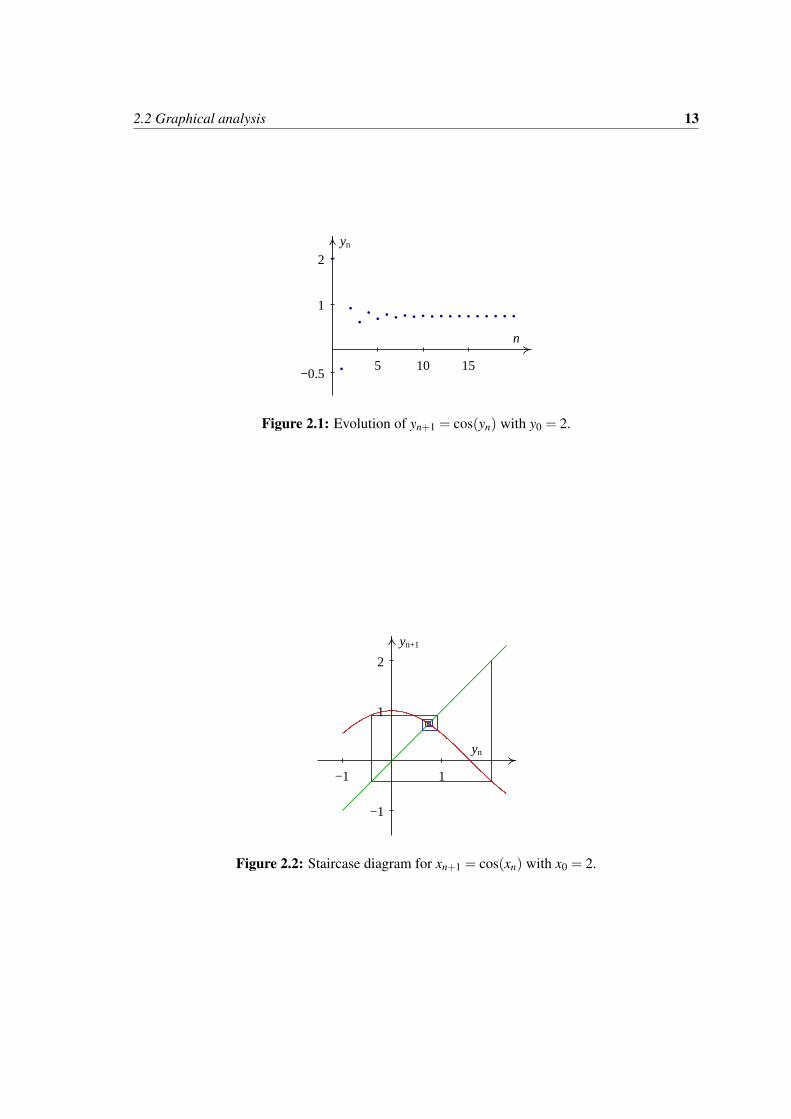
For instance, using y to identify the state variable in example 2.1, we have F(y) = cosy with initialvalue y0 = 2. To plot a graph with the first 20 terms, we use the commands:

(%i18) load("dynamics")$

(%i19) evolution(cos(y), 2, 20)$

The graph obtained in (%i19) is shown in figure 2.1.

Another type of diagram which will be very useful to analyze first-order discrete dynamical sys-tems is the so-called staircase diagram,2 which consists in plotting the functions y = F(x) andy = x, as well as an alternating sequence of horizontal and vertical segments joining the points(y0,y0), (y0,y1), (y1, y1), (y1,y2), and so on. For example, figure 2.2 shows the staircase diagram forthe sequence represented in figure 2.1

The function staircase, included in the additional package dynamics, plots staircase diagrams.That function needs the same three arguments as the function evolution; namely, function F(y)from the right-hand side of the difference equation 2.1, the initial value y0 and the number of stepsin the sequence. The independent variable in the expression for F should always be y. You might

1Maxima’s package dynamics was added in version 5.10; if you have an older version, you must upgrade it in orderto use that package.

2Also know as cobweb diagram.

2.2 Graphical analysis 13

n

yn

5 10 15

1

2

−0.5

Figure 2.1: Evolution of yn+1 = cos(yn) with y0 = 2.

yn

yn+1

1−1

1

2

−1

Figure 2.2: Staircase diagram for xn+1 = cos(xn) with x0 = 2.

14 Discrete dynamical systems

need to make the appropriate change if the state variable is something different from y in yourproblem.

The graph 2.2 was obtained with the command

(%i20) staircase(cos(y),2,8)$

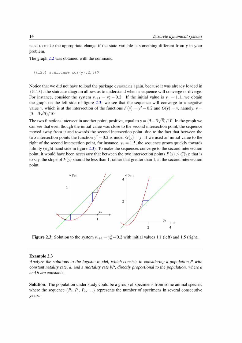
Notice that we did not have to load the package dynamics again, because it was already loaded in(%i18). the staircase diagram allows us to understand when a sequence will converge or diverge.For instance, consider the system yn+1 = y2

n − 0.2. If the initial value is y0 = 1.1, we obtainthe graph on the left side of figure 2.3; we see that the sequence will converge to a negativevalue y, which is at the intersection of the functions F(y) = y2 − 0.2 and G(y) = y, namely, y =(5−3

√5)/10.

The two functions intersect in another point, positive, equal to y = (5−3√

5)/10. In the graph wecan see that even though the initial value was close to the second intersection point, the sequencemoved away from it and towards the second intersection point, due to the fact that between thetwo intersection points the function y2− 0.2 is under G(y) = y. if we used an initial value to theright of the second intersection point, for instance, y0 = 1.5, the sequence grows quickly towardsinfinity (right-hand side in figure 2.3). To make the sequences converge to the second intersectionpoint, it would have been necessary that between the two intersection points F(x) > G(y); that isto say, the slope of F(y) should be less than 1, rather that greater than 1, at the second intersectionpoint.

yn

yn+1

1

1

yn

yn+1

2 4

2

4

Figure 2.3: Solution to the system yn+1 = y2n−0.2 with initial values 1.1 (left) and 1.5 (right).

Example 2.3Analyze the solutions to the logistic model, which consists in considering a population P withconstant natality rate, a, and a mortality rate bP, directly proportional to the population, where aand b are constants.

Solution: The population under study could be a group of specimens from some animal species,where the sequence P0, P1, P2, . . . represents the number of specimens in several consecutiveyears.

2.3 Fixed points 15

Let Pn represent the number of specimens at the beginning of period n. during that period of time,an average aPn new specimens are born, and bP2

n specimens die. Thus, in the beginning of the nextperiod, n+1, the population would be

Pn+1 = (a+1)Pn

(1− b

a+1Pn

)(2.7)

It is convenient to define a new variable yn = bPn/(a + 1). Thus, we obtain an equation with asingle parameter c = a+1

yn+1 = cyn(1− yn) (2.8)

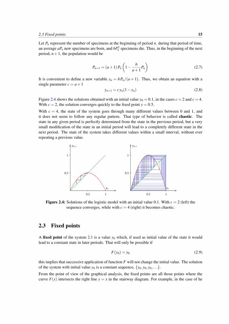
Figure 2.4 shows the solutions obtained with an initial value y0 = 0.1, in the cases c = 2 and c = 4.With c = 2, the solution converges quickly to the fixed point y = 0.5.

With c = 4, the state of the system goes through many different values between 0 and 1, andit does not seem to follow any regular pattern. That type of behavior is called chaotic. Thestate in any given period is perfectly determined from the state in the previous period, but a verysmall modification of the state in an initial period will lead to a completely different state in thenext period. The state of the system takes different values within a small interval, without everrepeating a previous value.

yn

yn+1

1

1

0.5

0.5

yn

yn+1

1

1

0.5

0.5

Figure 2.4: Solutions of the logistic model with an initial value 0.1. With c = 2 (left) thesequence converges, while with c = 4 (right) it becomes chaotic.

2.3 Fixed points

A fixed point of the system 2.1 is a value y0 which, if used as initial value of the state it wouldlead to a constant state in later periods. That will only be possible if

F(y0) = y0 (2.9)

this implies that successive application of function F will not change the initial value. The solutionof the system with initial value y0 is a constant sequence, y0,y0,y0, . . ..

From the point of view of the graphical analysis, the fixed points are all those points where thecurve F(x) intersects the right line y = x in the stairway diagram. For example, in the case of he

16 Discrete dynamical systems

logistic model, figure 2.4 shows that in the two cases c = 2 and c = 4 there are two fixed points,one of them at y = 0. We can use Maxima’s command solve to find the fixed points; in the casec = 4, the fixed points can be found in this way:

(%i21) flogistic: 4*y*(1-y);

(%o21) 4 (1 - y) y(%i22) fixed: solve(flogistic - y);

3(%o22) [y = -, y = 0]

4

The two fixed points are 0 and 0.75.

Let us consider a fixed point, where the curve F(x) intersects the straight line y = x, such that thederivative F ′(y) is bigger than 1 at that point. Namely, at the intersection point between the curveF(x) and the line y = x the curve F crosses from under the line, on the left, to over the line, on theright. Thus, if we plot the staircase diagram starting from a point near the fixed point, the sequencewill move away from the fixed point, describing a staircase in the staircase diagram. We call thatkind of fixed point a repulsive node.

If the derivative is negative and less than -1, the sequences will also move away from the fixedpoint, but alternating from side to side, describing a “cob web” in the staircase diagram. We callthat kind of fixed point a repulsive focus.

If the derivative of the function F near the fixed point has a value between 0 and 1, the sequencesthat start near the fixed point will approach it describing a staircase. That kind of fixed point iscalled an attractive node (an example of this case was already found in the left-hand side of 2.4).

If the derivative of the function F near the fixed point has a value between 0 and -1, the sequencesstarting near the point will approach it, describing a cob web that alternates from side to side inthe staircase diagram. That kind of point is called an attractive focus (an example of that kind ofpoint was already encountered in figure 2.2).

In summary, we have the following kinds of fixed points y0:

1. Attractive node, if 0 ≤ F ′(y0) < 1

2. Repulsive node, if F ′(y0) > 1

3. Attractive focus, if −1 < F ′(y0) < 0

4. Repulsive focus, if F ′(y0) <−1

If F ′(y0) equals 1 or -1, the situation is more complex: the fixed point could be either attractive orrepulsive, or even attractive from one side and repulsive from the other side.

Returning to our previous example of the logistic model (see (%i21) through (%o22) above), thevalue of the derivative of F at the fixed points is:

2.4 Periodic points 17

(%i23) dflogistic: diff(flogistic, y);

(%o23) 4 (1 - y) - 4 y(%i24) dflogistic, fixed[1];

(%o24) - 2(%i25) dflogistic, fixed[2];

(%o25) 4

Thus, in the case c = 4, both fixed points are repulsive. At y0 = 0 there is a repulsive node, andthere is a repulsive focus at y0 = 0.75.

2.4 Periodic points

If the sequence y0,y1,y2, . . . is a solution of the dynamical system

yn+1 = F(yn) (2.10)

any element in the sequence can be obtained from y0, applying the composed function Fn

yn = Fn(y0) = F(F(. . .(F︸ ︷︷ ︸n times

(y)))) (2.11)

A solution is dubbed a cycle of period 2, if it is a sequence of only two alternating values:y0,y1,y0,y1, . . .. The two points y0 and y1 are periodic points with period equal to 2. Sincey2 = F2(y0) = y0, it is necessary that F2(y0) = y0. Furthermore, since y3 = F2(y1) = y1 we alsohave F2(y1) = y1. Finally, since F(y0) = y1 6= y0, it is also necessary that F(y0) 6= y0, and sinceF(y1) = y0 6= y1, we also have F(y1) 6= y1.

Those conditions can be summarized by saying that two points y0 and y1 form a cycle of periodtwo if both of them are fixed points of the function F2(y), but none of them is a fixed point of thefunction F(y). Explained in a different way, if we calculate the fixed points of F2(y), all of thefixed points will appear, plus the periodic points of period 2 of functio F .

The cycle of period two will be attractive or repulsive according to the value of the derivative ofF2 at each point in the cycle.

To calculate the derivative of F2 at y0, we use the chain rule

(F2(y0))′ = (F(F(y0)))′ = F ′(F(y0))F ′(y0) = F ′(y0)F ′(y1) (2.12)

thus, the derivative of F2 takes the same value in the two points y0 and y1 of the cycle, and it isequal to the product of the derivatives of F in those two points.

Generalizing the definition a point y0 is part of a cycle of period m, if Fm(y0) = y0, but F j(y0) 6= y0for any j < m. The complete set of m points that make part of the cycle are

y0

18 Discrete dynamical systems

y1 = F(y0)y2 = F2(y0)

...

ym−1 = Fm−1(y0)

All those points are fixed points of Fm but they cannot be fixed points od F j, with j < m.

If the absolute value of the product of the derivative at the m points of the cycle:

m−1

∏j=0

F ′(y j) (2.13)

is greater than 1, then the cycle is repulsive; if the product is less than 1, the cycle is attractive, andif the product is identical to 1, the cycle could be either attractive or repulsive in different regions.

Example 2.4Find the cycles with period 2 for the logistic system

yn+1 = 3.1yn(1− yn)

and say whether they are attractive or repulsive.

Solution: We start by defining function F(y) and the composed function F2(y)

(%i26) flog: 3.1*y*(1-y)$

(%i27) flog2: flog, y=flog;

(%o27) 9.610000000000001 (1 - y) y (1 - 3.1 (1 - y) y)

The periodic points of period 2 will be among the solutions of the equation F2(y)− y = 0

(%i28) periodic: solve(flog2 - y);

sqrt(41) - 41 sqrt(41) + 41 21(%o28) [y = - -------------, y = -------------, y = --, y = 0]

62 62 31

The last two points, namely 0 and 21/31 are fixed points (the proof of that is left as an exercise forthe reader and can be done by solving the equation F(y) = y, or simply by showing the validity ofthat equation in each case).

The other two points must then form a cycle of period two; if we use any of them as initial value,the sequence will oscillate between those two points.

To find out whether the cycle is attractive or repulsive, we compute the product of the derivativeat the two points in the cycle

2.5 Solving equations numerically 19

(%i29) dflog: diff(flog, y);

(%o29) 3.1 (1 - y) - 3.1 y

(%i30) dflog, periodic[1], ratsimp, numer;

(%o30) - .3596875787352

(%i31) dflog, periodic[2], ratsimp, numer;

(%o31) - 1.640312421264802

(%i32) %o30*%o31;

(%o32) .5900000031740065

The absolute value of the product is less than 1, which implies that the cycle is attractive.

2.5 Solving equations numerically

Discrete, first-oder dynamical systems can be used for solving one-variable equations numerically.The problem to be solved consists on finding the roots of a real function f , namely, the values ofx that satisfy the equation

f (x) = 0 (2.14)

For example, suppose we want to find the values of x that solve the equation:

3x2− xcos(5x) = 6

That kind of equation cannot be solved analytically; it must be solved by numerical methods. Thenumerical methods to solve that equation consist on defining a dynamical system with convergentsequences which approach the solutions of the equation. In the following sections we will studytwo of those methods.

2.5.1 Iteration method

If the equation 2.14 can be written in the form

x = g(x) (2.15)

Its solutions are the fixed points of the dynamical system:

xn+1 = g(xn) (2.16)

20 Discrete dynamical systems

To find a fixed point, we choose an arbitrary initial point and calculate the evolution of the system.

Example 2.5Find the solution of the equation x = cosx

Solution: This equation is already given in a form that allows us to use the iteration method. Weuse the dynamical system with recurrence relation

xn+1 = cos(xn)

To find a fixed point, we choose an arbitrary initial point and calculate the evolution of the system

(%i33) x: 1$

(%i34) for i thru 15 do (x: float(cos(x)), print(x))$

0.540302305868140.857553215846390.654289790497780.793480358742570.701368773622760.763959682900650.722102425026710.750417761763760.731404042422510.744237354900560.735604740436350.741425086610110.737506890513240.740147335567880.73836920412232

The solution of the equation is approximately 0.74. This method was successful in this example,because the fixed point of the dynamical system chosen happened to be attractive. If the pointwere repulsive, the iteration method would have failed.

Example 2.6Find the square root of 5, using only additions, multiplications and divisions.

Solution: The square root of 5 is the positive solution of the equation

x2 = 5

2.5 Solving equations numerically 21

which can be written as:

x =5x

we solve the dynamical system associated to the function

f (x) =5x

It can be easily seen that for any initial value x0, different from√

5, the solution of that systemwill always be a cycle with period 2:

x0,5x0

,x0,5x0

, . . .

To escape from that cycle, and approach the fixed point at

√5, we can try to use the middle point:

xn+1 =12

(xn +

5xn

)That new system will converge quickly to the fixed point at

√5:

(%i35) x : 1$

(%i36) for i thru 7 do (x: float((x + 5/x)/2), print(x))$3.02.3333333333333342.2380952380952382.2360688956433632.2360679774999782.236067977499792.23606797749979

2.5.2 Newton’s method

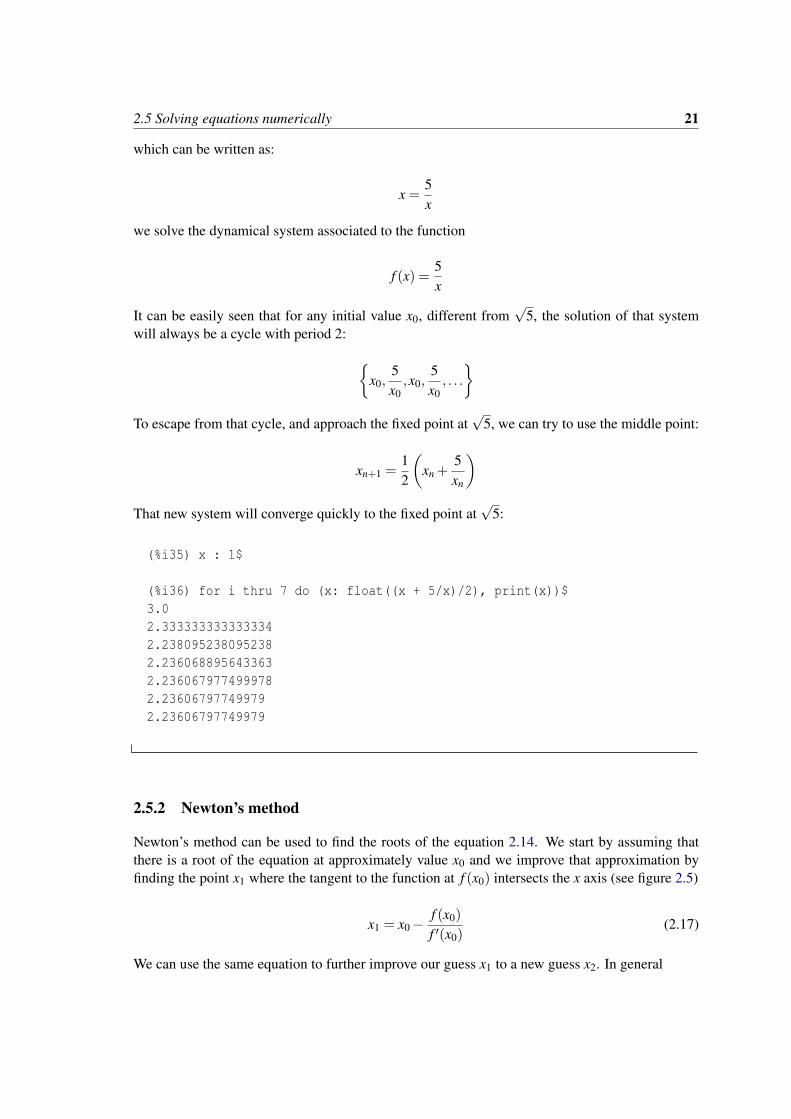
Newton’s method can be used to find the roots of the equation 2.14. We start by assuming thatthere is a root of the equation at approximately value x0 and we improve that approximation byfinding the point x1 where the tangent to the function at f (x0) intersects the x axis (see figure 2.5)

x1 = x0−f (x0)f ′(x0)

(2.17)

We can use the same equation to further improve our guess x1 to a new guess x2. In general

22 Discrete dynamical systems

xn+1 = xn−f (xn)f ′(xn)

(2.18)

x

f

x0x1

f(x0)

Figure 2.5: Newton’s method for finding roots of an equation.

It must be noticed that the roots of a continuous function f , points where f is zero, are fixed pointsof the dynamical system defined by equation 2.18 3.

The advantage of this method, over the iteration method, can be seen by using our analysis of thefixed points of a dynamical system. The function that generates the system 2.18 is

g(x) = 1− f (x)f ′(x)

(2.19)

the derivative of that function is

g′ = 1− ( f ′)2− f ′′ f( f ′)2 =

f ′′ f( f ′)2 (2.20)

at the fixed points, f vanishes. Thus, g′ will also vanish at the fixed points. Therefore, the fixedpoints of 2.18 will always be attractive. It means that if the initial point x0 is chosen close enoughto one of the roots of f , the sequence xn will approach it. The problem consists on finding whatclose enough means in each case.

To illustrate the method, we will solve example 2.6 once again, using Newton’s method.

The square root of 5 is one of the solutions of the equation x2 = 5. Hence, to find the square rootof 5 we can search for the positive root of the function

f (x) = x2−5

The derivative of that function isf ′(x) = 2x

substituting it into the recurrence relation 2.18, we obtain

xn+1 = xn−x2

n−52xn

=12

(xn +

5xn

)which is exactly the same sequence that we have already obtained and solved in the previoussection. However, in this case we did not need to introduce any clever tricks; we just applied thestandard method.

3If there are any regions where f and f ′ are both equal to zero, the roots will not be isolated points, but there willbe a whole interval with an infinite number of roots. In this section we will not study those kind of roots.

2.6 References 23

2.6 References

Some useful references, with a level similar to the one used here, are Chaos (Alligood et al., 1996),A First Course in Chaotic Dynamical Systems (Devaney, 1992) and Chaos and Fractals (Peitgenet al., 1992).

2.7 Multiple-choice questions

1. The state variable of a first-order, discretedynamical system takes on the values fromthe following sequence:3.4,6.8,7.2,5.1,6.8, ...what can be concluded about that system:

A. it does not have any cycles with periodless than 5.

B. it has a fixed point.

C. it is a chaotic system.

D. it has a cycle of period 3.

E. it has a cycle of period 2.

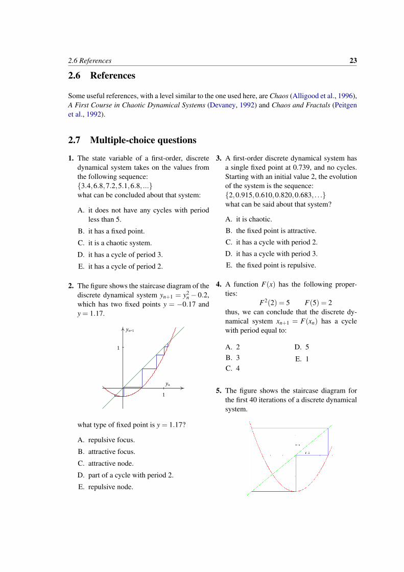
2. The figure shows the staircase diagram of thediscrete dynamical system yn+1 = y2

n − 0.2,which has two fixed points y = −0.17 andy = 1.17.

yn

yn+1

1

1

what type of fixed point is y = 1.17?

A. repulsive focus.

B. attractive focus.

C. attractive node.

D. part of a cycle with period 2.

E. repulsive node.

3. A first-order discrete dynamical system hasa single fixed point at 0.739, and no cycles.Starting with an initial value 2, the evolutionof the system is the sequence:2,0.915,0.610,0.820,0.683, . . .what can be said about that system?

A. it is chaotic.

B. the fixed point is attractive.

C. it has a cycle with period 2.

D. it has a cycle with period 3.

E. the fixed point is repulsive.

4. A function F(x) has the following proper-ties:

F2(2) = 5 F(5) = 2thus, we can conclude that the discrete dy-namical system xn+1 = F(xn) has a cyclewith period equal to:

A. 2B. 3C. 4

D. 5

E. 1

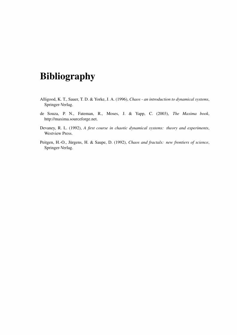
5. The figure shows the staircase diagram forthe first 40 iterations of a discrete dynamicalsystem.

24 Discrete dynamical systems

thus, we can conclude that the system has:

A. an attractive focus.

B. a repulsive focus.

C. a cycle with period 2.

D. a cycle with period 3.

E. a cycle with period 40.

2.8 Problems

1. The sequence obtained in this chapter to calculate square roots,

xn+1 =12

(xn +

axn

)was already known by the Sumerians, 4000 years ago. Using that method, calculate

√3,√

15and

√234. Use any positive initial value and represent the number a as a floating-point number

(for instance, 3.0), to force Maxima to give its results also as a floating-point number. In eachcase, compare the result with the value obtain using function sqrt() in Maxima.

2. Assume that the current whale population in the world is 1000 and that every year the normalincrease of the population (births minus deaths by natural causes) is 25%. Assuming that thenumber of whales killed by fishermen every year remained constant at 300 during the nextyears, how will the whale population evolve during the next 10 years?

3. Compute the first 10 terms of the sequence defined by the equation:

xn+1 = x2n−2

using the following initial values:

(a) x0 = 1

(b) x0 = 0.5

(c) x0 = 2

(d) x0 = 1.999

Discuss the behavior of the sequence in each case.

4. For each function in the following list, the point y = 0 makes part of a cycle for the systemyn+1 = F(yn). Determine the period of the cycle for each case and calculate the derivativeof the function in order to determine whether the cycle is attractive or repulsive. Draw thestaircase diagram of the sequence with initial value 0.

(a) F(y) = 1− y2

(b) F(y) =π

2cosy

(c) F(y) =−12

y3− 32

y2 +1

(d) F(y) = |y−2|−1

(e) F(y) =−4π

arctg(y+1)

5. Find the fixed points and the cycles with period 2 of the dynamical system:

yn+1 = F(yn)

and classify each point and cycle as attractive or repulsive, for each of the following cases:

2.8 Problems 25

(a) F(y) = y2− y2

(b) F(y) =2− y10

(c) F(y) = y4−4y2 +2

(d) F(y) =π

2siny

(e) F(y) = y3−3y

(f) F(y) = arctg(y)

In each case, start by drawing a staircase diagram using the function staircase and use it to findout the position of the fixed points and cycles; use the option domain to get a better overviewof the position of the fixed points. Then try to find the points analytically. In some cases thatwill not be possible and the result will have to be obtained approximately from the plots.

6. Considering the sequence xn+1 = |xn−2|

(a) Find all the fixed points. Show those points in a plot of the functions F(x) = |x−2| andG(x) = x.

(b) Explain the kind of sequence that will be obtained if x0 were a integer, either even or odd.

(c) Find the solution for the initial value 8.2.

(d) Find all the cycles with period two. Show all the points in those cycles in a plot of thefunctions F2(x) and G(x) = x.

7. Consider the function

F(x) =

2x , if x ≤ 14−2x , if x ≥ 1

(a) Show that F(x) is equivalent to 2−2|x−1|.(b) Plot, in the same graph, the functions F(x), F2(x), F3(x) and G(x) = x. What can you

conclude about the fixed points and cycles of the system xn+1 = F(xn)?

(c) Make a table or plot a graph of n against xn, between n = 0 and n = 100, for each of theinitial values 0.5, 0.6, 0.89, 0.893 and 0.1111111111. Discuss the results obtained.

(d) In the previous item, the sequence remains constant, starting at n = 55, for each of theinitial values. Compute again the sequences obtained in the last item, using the followingprogram, which uses higher numerical precision than the function evolution from thedynamics module.

evolution60(f, x0, n) :=block([x: bfloat(x0), xlist:[0, x0], fpprec: 60],for i thru ndo (x: ev(f), xlist: append(xlist, [i, float(x)])),openplot_curves([["plotpoints 1 nolines"], xlist]))

what can you conclude?

Index

Aattractive focus, 16attractive node, 16

Cchaotic, 15cycle, 17

Ddiff, 5difference equation, 9dynamics, 12, 14, 25

EEuler, 6evolution, 12, 25evolution equation, 9expand, 11

Ffixed point, 15

Iiteration method, 20

Kkill, 11

Llimit, 6list, 3

MMaxima, 1

NNewton’s method, 21nticks, 7numer, 6

OOhm’s law, 2

Pparametric, 6periodic points, 17plot2d, 5

Rrepulsive focus, 16repulsive node, 16roots, 19

Ssolve, 3, 5, 16staircase, 12staircase diagram, 12

Vvoltage-current characteristic, 3

Bibliography

Alligood, K. T., Sauer, T. D. & Yorke, J. A. (1996), Chaos - an introduction to dynamical systems,Springer-Verlag.

de Souza, P. N., Fateman, R., Moses, J. & Yapp, C. (2003), The Maxima book,http://maxima.sourceforge.net.

Devaney, R. L. (1992), A first course in chaotic dynamical systems: theory and experiments,Westview Press.

Peitgen, H.-O., Jurgens, H. & Saupe, D. (1992), Chaos and fractals: new frontiers of science,Springer-Verlag.