Introduction to Dynamical Systems - QMUL Mathsklages/mas424/lnotes_ds2007f.pdf · Introduction to...

Introduction to Dynamical Systems

Lecture Notes for MAS424/MTHM021

Version 1.2, 18/04/2008

Rainer Klages

School of Mathematical Sciences

Queen Mary, University of London

Notes for version 1.1 compiled by Phil Howard

c© Rainer Klages, Phil Howard, QMUL

Contents

1 Preliminaries . . . . . . . . . . . . . . . . . . . . . . . . . . . . . . . . . . . . . . . . . . . . . . . . . . . . . . . . . . . . . 5

I What is a dynamical system? 7

2 Examples of realistic dynamical systems. . . . . . . . . . . . . . . . . . . . . . . . . . . . . . . . . . . . 72.1 Driven nonlinear pendulum . . . . . . . . . . . . . . . . . . . . . . . . . . . 72.2 Bouncing ball . . . . . . . . . . . . . . . . . . . . . . . . . . . . . . . . . . . 92.3 Particle billiards . . . . . . . . . . . . . . . . . . . . . . . . . . . . . . . . . . 9

3 Definition of dynamical systems and the Poincare-Bendixson theorem. . . . . . . . 123.1 Time-continuous dynamical systems . . . . . . . . . . . . . . . . . . . . . . . 123.2 Time-discrete dynamical systems . . . . . . . . . . . . . . . . . . . . . . . . 163.3 Poincare surface of section . . . . . . . . . . . . . . . . . . . . . . . . . . . . 19

II Topological properties of one-dimensional maps 23

4 Some basic ingredients of nonlinear dynamics . . . . . . . . . . . . . . . . . . . . . . . . . . . . . . 244.1 Homeomorphisms and diffeomorphisms . . . . . . . . . . . . . . . . . . . . . 264.2 Periodic points . . . . . . . . . . . . . . . . . . . . . . . . . . . . . . . . . . 274.3 Dense sets, Bernoulli shift and topological transitivity . . . . . . . . . . . . . 294.4 Stability . . . . . . . . . . . . . . . . . . . . . . . . . . . . . . . . . . . . . . 35

5 Definitions of deterministic chaos . . . . . . . . . . . . . . . . . . . . . . . . . . . . . . . . . . . . . . . . . . 375.1 Devaney chaos . . . . . . . . . . . . . . . . . . . . . . . . . . . . . . . . . . . 375.2 Sensitivity and Wiggins chaos . . . . . . . . . . . . . . . . . . . . . . . . . . 385.3 Ljapunov chaos . . . . . . . . . . . . . . . . . . . . . . . . . . . . . . . . . . 395.4 Summary . . . . . . . . . . . . . . . . . . . . . . . . . . . . . . . . . . . . . 42

III Probabilistic description of one-dimensional maps 44

6 Dynamics of statistical ensembles. . . . . . . . . . . . . . . . . . . . . . . . . . . . . . . . . . . . . . . . . . 446.1 The Frobenius-Perron equation . . . . . . . . . . . . . . . . . . . . . . . . . 456.2 Markov partitions and transition matrices . . . . . . . . . . . . . . . . . . . 50

7 Measure-theoretic description of dynamics . . . . . . . . . . . . . . . . . . . . . . . . . . . . . . . . . 607.1 Probability measures . . . . . . . . . . . . . . . . . . . . . . . . . . . . . . . 607.2 Basics of ergodic theory . . . . . . . . . . . . . . . . . . . . . . . . . . . . . 69

Bibliography. . . . . . . . . . . . . . . . . . . . . . . . . . . . . . . . . . . . . . . . . . . . . . . . . . . . . . . . . . . . . . 75

4 Contents

1 Preliminaries

There exist two essentially different approaches to the study of dynamical systems, based onthe following distinction:

time-continuous nonlinear differential equations ⇋ time-discrete maps

One approach starts from time-continuous differential equations and leads to time-discretemaps, which are obtained from them by a suitable discretization of time. This path ispursued, e.g., in the book by Strogatz [Str94].1 The other approach starts from the study oftime-discrete maps and then gradually builds up to time-continuous differential equations,see, e.g., [Ott93, All97, Dev89, Has03, Rob95]. After a short motivation in terms of nonlineardifferential equations, for the rest of this course we shall follow the latter route to dynamicalsystems theory. This allows a generally more simple way of introducing the importantconcepts, which can usually be carried over to a more complex and physically realisticcontext.

As far as the style of these lectures is concerned, it is important to say that this course, andthus these notes, are presented not in the spirit of a pure but of an applied mathematician(actually, of a mathematically minded theoretical physicists). That is, we will keep technicalmathematical difficulties to an absolute minimum, and if we present any proofs they willbe very short. For more complicated proofs or elaborate mathematical subtleties we willusually refer to the literature. In other words, our goal is to give a rough outline of crucialconcepts and central objects of this theory as we see it, as well as to establish crosslinksbetween dynamical systems theory and other areas of the sciences, rather than dwellingupon fine mathematical details. If you wish, you may consider this course as an appliedfollow-up of the 3rd year course MAS308 Chaos and Fractals.

That said, it is also not intended to present an introduction to the context and historyof the subject. However, this is well worth studying, the field now encompassing overa hundred years of activity. The book by Gleick [Gle96] provides an excellent startingpoint for exploring the historical development of this field. The very recent book by Smith[Smi07] nicely embeds the modern theory of nonlinear dynamical systems into the generalsocio-cultural context. It also provides a very nice popular science introduction to basicconcepts of dynamical systems theory, which to some extent relates to the path we willfollow in this course.

This course consists of three main parts: The introductory Part I starts by exploring someexamples of dynamical systems exhibiting both simple and complicated dynamics. Wethen discuss the interplay between time-discrete and time-continuous dynamical systemsin terms of Poincare surfaces of section. We also provide a first rough classification ofdifferent types of dynamics by using the Poincare-Bendixson theorem. Part II introduces

1see also books by Arrowsmith, Percival and Richards, Guckenheimer and Holmes

6 1 Preliminaries

elementary topological properties of one-dimensional time-discrete dynamical systems, suchas periodic points, denseness and stability properties, which enables us to come up withrigorous definitions of deterministic chaos. This part connects with course MAS308 butpushes these concepts a bit further. Part III finally elaborates on the probabilistic, orstatistical, description of time-discrete maps in terms of the Frobenius-Perron equation.For this we need concepts like (Markov) partitions, transition matrices and probabilitymeasures. We conclude with a brief outline of essentials of ergodic theory. If you areinterested in further pursuing these topics, please note that there is a strong research groupat QMUL particularly focusing on (ergodic properties of) dynamical systems with crosslinksto statistical physics.2

The format of these notes is currently somewhat sparse, and it is expected that they willrequire substantial annotation to clarify points presented in more detail during the actuallectures. Please treat them merely as a study aid rather than a comprehensive syllabus.

2see http://www.maths.qmul.ac.uk/˜mathres/dynsys for further information

Part I

What is a dynamical system?

2 Examples of realistic dynamicalsystems

2.1 Driven nonlinear pendulum

Figure 2.1 shows a pendulum of mass M subject to a torque (the rotational equivalent ofa force) and to a gravitational force G. You may think, for example, of a clock pendulumor a driven swing. The angle with the vertical in a positive sense is denoted by θ = θ(t),where t ∈ R holds for the time of the system, and we choose −π ≤ θ < π.

θ

G

Rod

M

TorquePivot

Figure 2.1: Driven pendulum of mass M with a torque applied at the pivot and subject togravity.

Without worrying too much about how one can use physics to obtain an equation of motionfor this system starting from Newton’s equation of motion, see [Ott93, Str94] for suchderivations, we move straight to the equation itself and merely indicate whence each termarises:

8 2 Examples of realistic dynamical systems

Equation of motion: θ + νθ + sin θ = A sin (2πft)↑ ↑ ↑ ↑

Balance of forces: inertia + friction + gravity = periodic torque, (2.1)

where for sake of simplicity we have set the mass M equal to one. Here we write θ := dθdt

todenote the derivative of θ with respect to time, which is also sometimes called the angularvelocity. In (2.1) θ is an example of a dynamical variable describing the state of the system,whereas ν, A, f are called control parameters. Here ν denotes the friction coefficient, A theamplitude of the periodic driving and f the frequency of the driving force. In contrast todynamical variables, which depend on time, the values for the control parameters are chosenonce for the system and then kept fixed, that is, they do not vary in time. Equation (2.1)presents an example of a driven (driving force), nonlinear (because of the sine function,sin x ≃ x − x3/3!), dissipative (because of driving and damping) dynamical system.

It is generally impossible to analytically solve complicated nonlinear equations of motionsuch as (2.1). However, they can still be integrated by numerical methods (such as Runge-Kutta integration schemes), which allows the production of simulations such as the onesthat can be explored in “The Pendulum Lab”, a very nice interactive webpage [Elm98].Playing around with varying the values of control parameters there, one finds the followingfour different types of characteristic behaviour: This systems has already been studied inmany experiments, even by high school pupils!

ω

θ

ω

θ

ω

θ

ω

θ

(1)

(4)(3)

(2)

Figure 2.2: Plots of four different types of motion of the driven nonlinear pendulum (2.1)in the (θ, ω)-space under variation of control parameters.

1. No torque A = 0, no damping ν = 0, small angles θ ≪ 1 leading to

θ + θ = 0 . (2.2)

2.2 Bouncing ball 9

This system is called the harmonic oscillator, and the resulting dynamics is known aslibration. If we represent the dynamics of this system in a coordinate system where weplot θ and the angular velocity ω := θ as functions of time, we obtain pictures whichlook like the one shown in Fig. 2.2 (a).

2. same as 1. except that θ can be arbitrarily large, −π ≤ θ < π: Fixed points exist atθ = 0 (stable) and θ = π (unstable). If the initial condition θ(0) = π is taken withnon-zero initial velocity ω 6= 0, continual rotation is obtained; see Fig. 2.2 (b).

3. same as 2. except that the damping is not zero anymore, ν 6= 0: The pendulum comesto rest at the stable fixed point θ = 0 for t → ∞. This is represented by some spiralingmotion in Fig. 2.2 (c).

4. same as 3. except that now we have a periodic driving force, that is, A, f 6= 0: In thiscase we explore the dynamics of the full driven nonlinear pendulum equation (2.1).We observe a ‘wild’, rather unpredictable, chaotic-like dynamics in Fig. 2.2 (d).

We conclude this discussion by mentioning that the driven nonlinear pendulum is a paradig-matic example of a non-trivial dynamical system, which also displays chaotic behavior. Itis found in many physical and other systems such as in Josephson junctions (which aremicroscopic semi-conductor devices), in the motion of atoms and planets and in biologicalclocks. It is also encountered in many engineering problems.

2.2 Bouncing ball

Another seemingly simple system displaying non-trivial behavior is the bouncing ball schemat-ically depicted in Fig. 2.3: The figure shows an elastic ball of mass M falling under a gravita-tional force G by bouncing off a plate that vibrates with amplitude A and frequency f , thusallowing transfer of energy to and from the ball system. Additionally, the ball experiencesa friction ν at the collision.Without going into further detail here, such as writing down the systems’ equations ofmotion, we may mention that for certain values of the control parameters this systemexhibits simple periodic behavior in form of ‘frequency locking’, where the periodic motionof the bouncing ball and of the vibrating plate are in phase. This is like a ping-pong ballhopping vertically on your oscillating table tennis racket. In other words, here we have acertain type of ‘resonance’. However, under smooth variation of control parameters such asamplitude or frequency of the driving one typically observes a transition to periodic motionof increasingly higher order (called “bifurcations”) until the motion eventually becomescompletely irregular, or “chaotic”.1

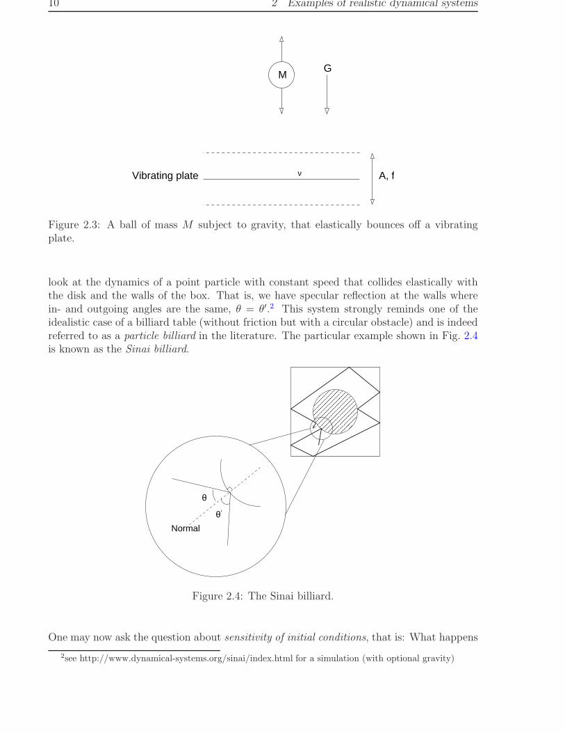
2.3 Particle billiards

A third example is provided by the following system, see Fig. 2.4: Let us consider a harddisk of radius r, whose centre is fixed in the middle of a square box in the plane. We now

1see N.Tufillaro’s webpage http://www.drchaos.net/drchaos/bb.html or the one by P.Pieranskihttp://fizyka.phys.put.poznan.pl/˜pieransk/BouncigBall.html for further details; see also the book by Teland Gruiz

10 2 Examples of realistic dynamical systems

A, f

MG

Vibrating plate ν

Figure 2.3: A ball of mass M subject to gravity, that elastically bounces off a vibratingplate.

look at the dynamics of a point particle with constant speed that collides elastically withthe disk and the walls of the box. That is, we have specular reflection at the walls wherein- and outgoing angles are the same, θ = θ′.2 This system strongly reminds one of theidealistic case of a billiard table (without friction but with a circular obstacle) and is indeedreferred to as a particle billiard in the literature. The particular example shown in Fig. 2.4is known as the Sinai billiard.

��

��

Normal

θ’

θ

Figure 2.4: The Sinai billiard.

One may now ask the question about sensitivity of initial conditions, that is: What happens

2see http://www.dynamical-systems.org/sinai/index.html for a simulation (with optional gravity)

2.3 Particle billiards 11

to two nearby particles in this billiard (which do not interact with each other) with slightlydifferent directions of their initial velocities? Since at the moment no computer simulationof this case is available to us, we switch to a slightly more complicated dynamical systemas displayed in Fig. 2.5, where we can numerically explore this situation [Miy03].

GM

Figure 2.5: A billiard where a point particle bounces off semicircles on a plate.

The dynamical system is defined as follows: we have a series of semicircles periodicallycontinued onto the line, which may overlap with each other. A point particle of mass Mnow scatters elastically with these semicircles under the influence of a gravitational forceG. In the simulation we study the spreading in time of an ensemble of particles startingfrom the same point, but with varied velocity angles. The result is schematically depictedin Fig. 2.6: We see that there are two important mechanisms determining the dynamics ofthe particles, namely a stretching, which initially is due to the choice of initial velocities butlater on also reflects the dispersing collisions at the scatterers, and a folding at the collisions,where the front of propagating particles experiences cusps. This sequence of “stretch” and“fold” generates very complicated structures in the position space of the system, which looklike mixing paint.

FoldStretch

Figure 2.6: Schematic representation of the stretch and fold mechanism of an ensemble ofparticles in a chaotic dynamical system.

As we shall see later in this course, this is one of the fundamental mechanisms of what iscalled “chaotic behavior” in nonlinear dynamical systems. The purpose of these lecturesis to put the handwaving assessment of the behavior illustrated above for some “realistic”dynamical systems onto a more rigorous mathematical basis such that eventually we can

answer the question what it means to say that a system exhibits “chaotic” dynamics. Tothe end of this course we will also consider the dynamics of statistical ensembles of particlessuch as in the simulation.

3 Definition of dynamical systems andthe Poincare-Bendixson theorem

Definition 1 [Las94, Kat95]1 A dynamical system consists of a phase (or state) space Pand a family of transformations φ

t: P → P , where the time t may be either discrete, t ∈ Z,

or continuous, t ∈ R. For arbitrary states x ∈ P the following must hold:

1. φ0(x) = x identity and

2. φt(φ

s(x)) = φ

t+s(x) ∀t, s ∈ R additivity

In other words, a dynamical system may be understood as a mathematical prescription forevolving the state of a system in time [Ott93, All97]. Property 2 above ensures that thetransformations φ

tform an Abelian group. As an exercise, you may wish to look up different

definitions of dynamical systems on the internet.

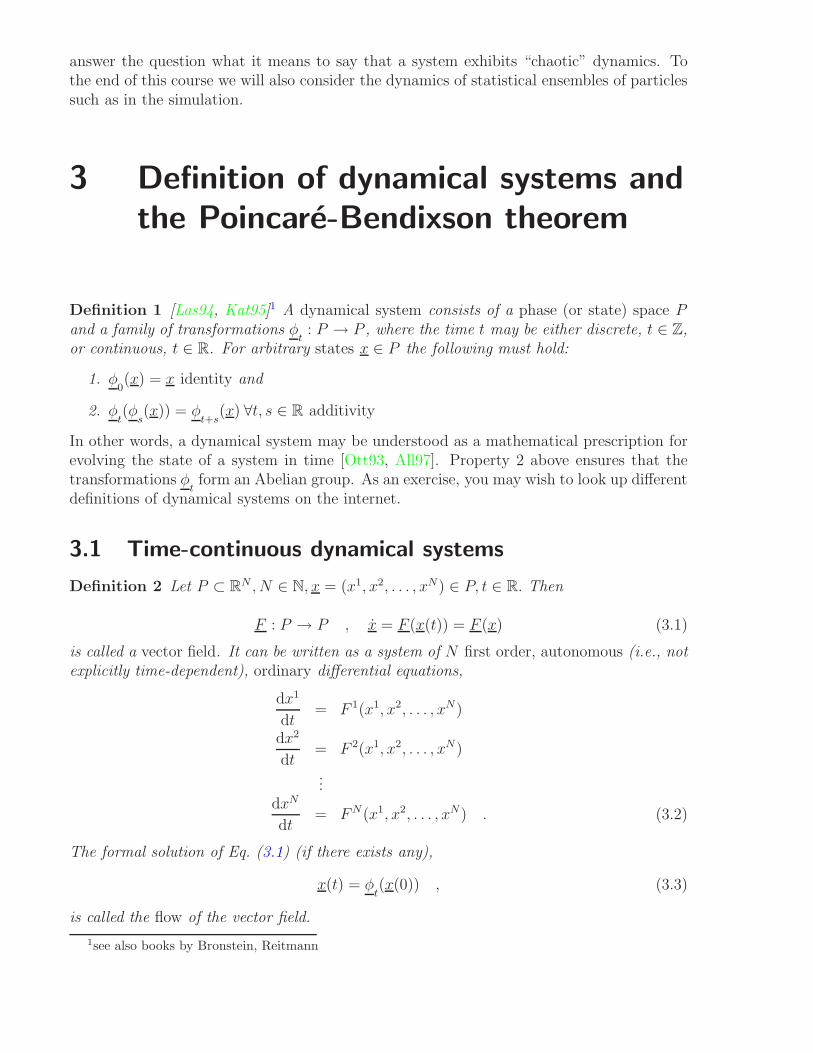
3.1 Time-continuous dynamical systems

Definition 2 Let P ⊂ RN , N ∈ N, x = (x1, x2, . . . , xN) ∈ P, t ∈ R. Then

F : P → P , x = F (x(t)) = F (x) (3.1)

is called a vector field. It can be written as a system of N first order, autonomous (i.e., notexplicitly time-dependent), ordinary differential equations,

dx1

dt= F 1(x1, x2, . . . , xN)

dx2

dt= F 2(x1, x2, . . . , xN)

...dxN

dt= F N(x1, x2, . . . , xN) . (3.2)

The formal solution of Eq. (3.1) (if there exists any),

x(t) = φt(x(0)) , (3.3)

is called the flow of the vector field.

1see also books by Bronstein, Reitmann

3.1 Time-continuous dynamical systems 13

Here φtis the transformation that we have already encountered in Definition 1 above. Note

that this does not answer the question of how to construct the flow for arbitrary initialconditions x(0).

Definition 3 A single path in phase space followed by x(t) in time is called the trajectoryor orbit of the dynamical system.2

See Fig. 3.1 for an example.

x3

x2

x1

x(0)

x(t)

Figure 3.1: Example of a trajectory in 3-dimensional phase space (note that the trajectoryis not supposed to cross itself).

In the following we will assume the existence and uniqueness of solutions of the vector fieldF . A proof of this exists if F is smooth (continuously differentiable, C1) [Str94].

Corollary 1 For smooth F two distinct trajectories cannot intersect, nor can a single tra-jectory cross itself for t < ∞.

Proof: Assume a single trajectory crosses itself, see Fig. 3.2. Starting with the initialcondition at the point of intersection there are two choices of direction to proceed in, whichcontradicts uniqueness. The same argument applies to two distinct trajectories. q.e.d.

Figure 3.2: A trajectory that crosses itself.

If ∃ uniqueness, x(0) determines the outcome of a flow after time t: we have what is calleddeterminism.

2In this course we use both words synonymously.

14 3 Definition of dynamical systems and the Poincare-Bendixson theorem

One may now ask about the general ‘character’ of a flow φt(x), intuitively speaking: Is it‘simple’ or ‘complicated’? In the following we give a first, rather qualitative answer.

Definition 4 We call a flow simple if for t → ∞ all x(t) are either fixed points x =constant, respectively x = 0, or periodic orbits, i.e., closed loops x(t + τ) = x(t), τ ∈ R.

Two examples of fixed points are shown in Figs. 3.3: In both cases the fixed point is locatedat the origin of the coordinate system in the two-dimensional plane. However, if we lookat initial conditions in an environment around these fixed points and how the trajectorydetermined by it evolves in time, we may observe different types of behavior: For example, inone case the trajectory ‘spirals in’ to the fixed point by approaching it time-asymptotically,whereas in the other case the trajectory ‘spirals out’.We remark that these are by far not the only cases of possible dynamics [Str94]. So we seethat a fixed point, apart from its mere existence, can have a very different impact onto itsenvironment: In the first case we speak of a stable fixed point, whereas in the second casethe fixed point is said to be unstable.

x2

x1

x2

x1

Stable fixed point Unstable fixed point

Figure 3.3: stable and unstable fixed points

The same reasoning applies to the simple example of a periodic orbit shown in Fig. 3.4: Theleft hand side depicts a circular periodic orbit. However, if we choose initial conditions thatare not on this circle we may observe, for example, the behavior illustrated on the righthand side of this figure: trajectories ‘spiral in’ onto the periodic orbit both from the interiorof the circle and from the exterior. An isolated closed trajectory such as this periodic orbitis called a limit cycle, which in this case is stable.Of course, as for the fixed point the opposite case is also possible, that is, the limit cycle isunstable if all nearby trajectories spiral out (you may wish to draw a figure of this). Thedetailed determination and classification of fixed points and periodic orbits is in the focusof what is called linear stability analysis in the literature, see [Ott93, Str94] in case of flows.For maps we will learn right this later in the course.

Definition 5 We call a flow complicated if it is not simple.

Typically, such a flow cannot be calculated analytically anymore, because it cannot be rep-resented in a simple functional form. In this case solutions can only be obtained numerically.Later on we will introduce ‘chaos’ as a subset of complicated solutions.3

3If ‘chaos’ defines a subset of complicated dynamics, this leaves the possibility of solutions that are

3.1 Time-continuous dynamical systems 15

x2

x1

x2

x1

Limit cycle

Figure 3.4: left: circular periodic orbit; right: approach to this orbit as a limit cycle

One may now ask the further question of how large the dimensionality N of the phase spacehas to be for complicated behaviour to be possible. The answer is given in terms of thefollowing important theorem:[Str94, Rob95]4

Theorem 1 (Poincare-Bendixson) Let x = F (x) be a smooth vector field acting on an openset containing a closed, bounded set R ⊂ R2, which is such that all trajectories starting inR remain in R. Then any trajectory starting in R is either a fixed point or a periodic orbit,or it spirals to one as t → ∞.

The proof of this theorem is elaborate and goes beyond the scope of this course. It is basedon the idea of uniqueness of solutions and that trajectories cannot cross each other; see, e.g.,[All97]. Under these conditions, the different topology in two and three dimensions plays acrucial role as is demonstrated in Fig. 3.5. See also [Str94] for more detailed discussions.

2d 3d

Figure 3.5: Trajectories in 2-d (left) cannot cross whereas in 3-d (right), they can.

Corollary 2 Let F (x) ∈ RN and the conditions of the Poincare-Bendixson theorem befullfilled. Then N ≤ 2 ⇒ solutions simple. Consequently, N ≥ 3 ⇒ ‘anything can happen’,i.e., complicated solutions are possible.

This raises the question of how to check these statements for a given differential equation,which we discuss for an example:

neither simple nor chaotic but nevertheless complicated. Such ‘weakly chaotic motion’ is a very active topicof recent research, see, e.g., Section 17.4 of [Kla07].

4see also a book by Hilborn


Example 1 Let us revisit the driven nonlinear pendulum that we have seen before,

θ + νθ + sin θ = A sin(2πft) .

Rewrite this dynamical system in the form of a vector field by using

x1 := θ, x2 := θ, x3 := 2πft .

The ‘trick’ of incorporating the time dependence of the differential equation as a thirdvariable allows us to make the vector field autonomous leading to

x1 = θ = −νx1 − sin x2 + A sin x3

x2 = x1

x3 = 2πf . (3.4)

Therefore N = 3: complicated dynamics is possible, as we have indeed seen in the simula-tions.

3.2 Time-discrete dynamical systems

Definition 6 Let P ⊂ RN , N ∈ N, xn ∈ P, n ∈ Z. Then

M : P → P , xn+1 = M(xn) (3.5)

is called a time-discrete map. xn+1 = M(xn) are sometimes called the equations of motionof the dynamical system.

Choosing the initial condition x0 determines the outcome after n discrete time steps (hencedeterminism) in the following way:

x1 = M(x0) = M 1(x0),

x2 = M(x1) = M(M(x0)) = M 2(x0)( 6= M(x0)M(x0)!).

⇒ Mm(x0) := M ◦ M ◦ · · ·M(x0)︸︷︷︸

m-fold composed map

. (3.6)

In other words, for maps the situation is formally simpler than for differential equations: ∃ aunique (why?) solution to the equations of motion in form of xn = M(xn−1) = . . . = Mn(x0).This is the counterpart of the flow for time-continuous systems.

Example 2 [Ott93] For N = 1 let zn ∈ N0 be the number of insects hatching out of eggsin year n ∈ N0. Let r > 0 be the average number of eggs laid per insect. In an (for theinsects) ‘ideal’ case we have

zn+1 = rzn = r2zn−1 = . . . = rn+1z0 = exp((n + 1) ln r)z0 , (3.7)

where we assume that insects live no longer than for one year. This straightforwardly impliesfor r > 1 an exponentially increasing and for r < 1 an exponentially decreasing population.

3.2 Time-discrete dynamical systems 17

In 1798 Malthus proposed to incorporate the effect of enemies, or overcrowding, by replacingthe control parameter r through the logistic growth r(1− zn

z), where z models a limited food

supply with 0 ≤ zn ≤ z. That is, if zn = z the food is exhausted and all insects die.Replacing r after the first equal sign of Eq. (3.7) above leads to the new equation

zn+1 = rzn(1 − zn

z) . (3.8)

Dividing both sides by z and defining the new variable xn := zn

zyields the famous logistic

map

xn+1 = rxn(1 − xn) , (3.9)

where here we restrict ourselves to 0 ≤ xn ≤ 1 , 0 < r ≤ 4.

How do we get information about the dynamics of this map? We could look, for example, atthe set of all iterates for a given initial condition x0, i.e. {x0, x1, x2, . . . , xn}, which definesthe trajectory or orbit of M(x0).Note that the same definition carries over to N -dimensional maps. However, in one dimen-sion we have a nice graphical representation of the trajectory in form of the cobweb plot, aswe may demonstrate for our above example:

Example 3 Cobweb plot for the logistic map restricted to the parameter range 1 < r < 2and for 0 ≤ x ≤ 1, see Fig. 3.6.

x0

y=x

M

y

xx1 x=1/2

y =M(x0)

y=x1

x0

unstablefixed point

x1 xsx2

y

x

stable fixed point

Figure 3.6: left: first step of a cobweb plot for the logistic map with 1 < r < 2; right:magnification of the left hand side with the result for the iterated procedure.

Constructing a cobweb plot for a map proceeds in five steps according to the followingalgorithm:

1. Choose an initial point x0 and draw a vertical line until it intersects the graph of thechosen map M(x). The point of intersection defines the value y = M(x0) of the mapafter the first iteration.

2. By using Eq. (3.5) we now identify y with the next position in the domain of the mapat time step n = 1 which leads to x1 = y.


3. This is represented in the figure by drawing a horizontal line from the previous pointof intersection until it intersects with the diagonal y = x.

4. Drawing a vertical line from the new point of intersection down to the x-axis makesclear that we have indeed graphically obtained the new position x1 on the abscissa.

5. However, in practice this last vetical line is neglected for making a cobweb plot. In-stead, we immediately construct the next iterate by repeating step 1 to 3 discussedabove for the new starting point x1 instead of x0, and so on.

In summary, for a cobweb plot we continuously alternate between vertical and horizontallines that intersect with the graph of the given map and the diagonal; see also p.5 of [All97]and [Has03] for details.

Definition 7 x is a fixed point of M if x = M(x).

For our one-dimensional example of the logistic map our cobweb plot Fig. 3.6 immediatelytells us that we have two fixed points, one at xu = 0 and another one at a (yet unspecified)larger value xs. Interestingly, the plot furthermore suggests that all points in the neigh-bourhood of xu move away from this fixed point and converge to xs. Hence, we may call xu

an unstable or repelling fixed point whereas we classify xs as being stable or attracting.In other words, a cobweb plot yields straightforwardly information both about the existenceof fixed points, which in one dimension are just the intersections x = M(x), and theirstability. Of course, the above statement provides only a qualitative assessment of thestability of fixed points. We will make this mathematically rigorous later on.

Definition 8 A map M is called invertible if ∃ an inverse M−1 with xn = M−1(xn+1).

Example 4

1. The logistic map is not invertible, since one image has two preimages, as you mayconvince yourself by a simple drawing.

2. Let us introduce the two-dimensional map

xn+1 = f(xn) − kyn , k 6= 0

yn+1 = xn . (3.10)

Here f(x) is just some function; as an example, let us choose f(x) = A − x2, A ∈ R.Eq. (3.10) together with this f(x) defines the famous Henon map (1976), derived fromthe (Hamiltonian) equations of motion for a star in a galaxy (1964) [Ott93].

Let us try to invert this mapping: We get

xn = yn+1

yn =1

k(f(xn) − xn+1)

=1

k(f(yn+1) − xn+1) , (3.11)

so we can conclude that the map is invertible.

3.3 Poincare surface of section 19

We may now be wondering whether there is any condition on N for the existence of ‘com-plicated solutions’ in time-discrete maps, in analogy to Corollary 2 for time-continuousdynamical systems. The answer is given as follows:

Corollary 3 [Ott93] (Poincare-Bendixson discretized) Let xn+1 = M(xn) be a smooth mapacting on an open set containing a closed, bounded set R ⊂ RN , which is such that alltrajectories starting in R remain in R. Let us look at trajectories starting in R for n → ∞.Let M be invertible. Then N = 1 ⇒ solutions simple. Consequently, N ≥ 2 ⇒ complicatedsolutions are possible. Let M be noninvertible. Then complicated solutions are alwayspossible.

So the discretized Poincare-Bendixson theorem leaves us with the possibility that the dy-namics even of simple one-dimensional maps is non-trivial, which is the reason why we aregoing to study them in detail.If you compare this Corollary with the previous one for flows, you will observe a reductionof the condition on the dimensionality N , implying regular dynamics, by one for invertiblemaps and by two for noninvertible maps in comparison with flows. This is no coincidenceas we will show in the following section. For a proof in case of invertible one-dimensionalmaps see [Has03, Kat95].

Example 5

1. Consider the logistic map Eq. (3.9) for 0 < r ≤ 4. It is smooth, defined on a compactset but not invertible, hence complicated solutions are possible.

2. Consider Henon’s map Eq. (3.10) for smooth f(x). This map is smooth, however,whether the time asymptotic dynamics is defined on a closed, bounded set R is notclear. On the other hand, the map is invertible and N = 2, hence complicated solutionsare in any case possible.

3.3 Poincare surface of section

A Poincare surface of section enables the reduction of an N -dimensional flow to an (N −1)-dimensional map. There exist two basic types:The first one is the Poincare surface of section in space. Fig. 3.7 shows an example for aflow defined by x = F (x) in N = 3-dimensional space.Let us consider the case, e.g., x3 = K, where K is a constant chosen by convenience. ThePoincare map for this system is then defined uniquely by the iteration

(x1

n+1

x2n+1

)

= M

(x1

n

x2n

)

(3.12)

from the nth to the (n + 1)st piercing under the condition that x3 = K is kept fixed.This definition appears to be fairly simple, however, there are at least two subtleties: Firstly,it is quite easy to produce a Poincare surface of section for a given differential equation nu-merically, but only in exceptional cases can the corresponding Poincare map be obtainedanalytically. Secondly, if the times τ between two piercings are constant, then some triv-ial information about the dynamical system is conveniently separated out by producing a


B(n+1)

C(n+2)

A(n)

x1

x3

x2

K

Figure 3.7: A continuous trajectory in space pierces the plane x3 = K at several points atdiscrete time n.

Poincare surface of section. However, most often there is no reason why τ should be con-stant. If this is not the case, the complete dynamics is defined by what is called a suspendedflow, or suspension flow,

xn+1 = M(xn) , xn ∈ RN−1 (3.13)

tn+1 = tn + T (xn) , T : RN−1 → R (3.14)

Eq. (3.14) is called the first-return time map.5 This allows some idea of how the Poincare-Bendixson theorem 1 applies to reduced-dimension discrete systems: The above suspendedflow still provides an exact representation of the underlying time-continuous dynamicalsystem. However, if we refer only to the first Eq. (3.13) by neglecting the second Eq. (3.14),as we did before, we reduce the dimensionality of the whole dynamical system by one.Of course we could also consider the whole suspended flow Eqs. (3.13),(3.14) as an N -dimensional map, however, the set on which Eq. (3.14) is defined is always unbounded andhence we could not relate to the Poincare-Bendixson theorem.Still, by construction our Poincare map Eq. (3.13) is invertible. However, if we neglect anysingle component of the vector in Eq. (3.13), implying that we further reduce the phase spacedimensionality by one, the resulting map will become noninvertible, because we have lostsome information. Hence, in view of the Poincare-Bendixson theorem 1 it is not surprisingthat despite their minimal dimensionality, one-dimensional noninvertible maps can exhibitcomplicated time-asymptotic behavior.

5Obviously, this equation then replaces the dynamics for the eliminated phase space variable, however,the detailed relation between these two different quantities is typically non-trivial [Gas98, Kat95].

3.3 Poincare surface of section 21

A second version of a Poincare map is obtained by a Poincare surface of section in time. Forthis purpose, we sample a time-continous dynamical system not with respect to a constraintin phase space but at discrete times tn = t0 + nτ, n ∈ N. In this case, the map determiningEq. (3.14) of the suspended flow boils thus down to T (xn) = nτ : We have what is called astroboscopic sampling of the phase space.

This variant is very convenient for dynamical systems driven by periodic forces such as,for example, our nonlinear pendulum Eq. (2.1) (why?). However, we wish to illustrate thistechnique for a simpler system, where this is easier to see. This system provides a rareexample for which the Poincare map can be calculated analytically. In order to do so, wefirst need to learn about a mathematical object called the (Dirac) ‘δ-function’, which wemay introduce as follows.

We are looking for a ‘function’ having the following properties:

δ(x) :=

{0 , x 6= 0∞ , x = 0

(3.15)

For example, think of the sequence of functions defined by

δγ(x) :=1

γ√

2πexp(− x2

2γ2) (3.16)

as shown in Fig. 3.8. It is not hard to see that in the limit of γ → 0 this sequence has thedesired properties, that is, δγ(x) → δ(x) (γ → 0).

x

Y γ 0γ3

γ2

γ1

Figure 3.8: A sequence of functions approaching the δ-function.

We remark that many other representations of the δ-function exist. Strictly speaking the‘δ-function’ is not a function but rather a functional, respectively a distribution defined ona specific (Schwartz) function space.6

6A nice short summary of properties of the δ-function, written from a physicist’s point of view, is given,for example, in the German version of the book by F.Reif, Statistische Physik und Theorie der Warme, seeAppendix A.7.


Two important properties of the δ-function that we will use in the following are its normal-ization,

∀ǫ > 0

∫ ǫ

−ǫ

dx δ(x) = 1 , (3.17)

and that for some integrable function f(x)

∫ ∞

−∞

dx f(x)δ(x) = f(0) . (3.18)

We are now prepared to discuss the following example:

Example 6 The kicked rotorA rotating bar of inertia I and length l suffers kicks of strength K/l applied periodically attime steps t = 0, τ, 2τ, . . . , τ ∈ R, see Fig. 3.9.

θ

length l, ’inertia’

kicks of strength_

I

no gravity

frictionless pivot

Kl

Figure 3.9: The kicked rotor.

The equation of motion for this dynamical system is straightforwardly derived from physicalarguments [Ott93], however, we just state it here in form of

θ = k sin θ∞∑

m=0

δ(t − mτ) , (3.19)

where the dynamical variable θ describes the turning angle and k := K/I is a controlparameter. As before we can rewrite this differential equation as a vector field,

θ = ω (3.20)

ω = k sin θ∞∑

m=0

δ(t − mτ) . (3.21)

According to Eq. (3.21) ω is constant during times t 6= mτ between the kicks but changesdiscontinuously at the kicks, which take place at times t = mτ . Eq. (3.20) then implies thatθ ∼ t between the kicks by changing continuously at the kicks, reflecting the discontinuouschanges in the slope ω.

Let us now construct a suitable Poincare surface of section in time for this dynamical system.Let us define θn := θ(t) and ωn := ω(t) at t = nτ + 0+, where 0+ is a positive infinitesimal.That is, we look at both dynamical variables right after each kick. We then integrateEq. (3.20) through the δ-function at t = (n + 1)τ leading to

∫ (n+1)τ+0+

nτ+0+

dt θ = θn+1 − θn = ωnτ (3.22)

The same way we integrate Eq. (3.21) to

ωn+1 − ωn = k

∫ (n+1)τ+0+

nτ+0+

dt sin θ∑

m

δ(t − mτ) = k sin θn+1 . (3.23)

For the special case τ = 1 we arrive at

θn+1 = θn + ωn (3.24)

ωn+1 = ωn + k sin θn+1 . (3.25)

This two-dimensional mapping is called the standard map, or sometimes also the Chirikov-Taylor map. It exhibits a dynamics that is typical for time-discrete Hamiltonian dynamicalsystems thus serving as a standard example for this class of systems [Ott93].7 For conve-nience, the dynamics of (θn, ωn) is often considered mod 2π. We remark in passing thatEqs. (3.24),(3.25) can also be derived from a toy model for cyclotron dynamics, wherea charged particle moves under a constant magnetic field and is accelerated by a time-dependent voltage drop.8

We may now further reduce the kicked rotor dynamics by feeding Eq. (3.24) into Eq. (3.25)leading to

ωn+1 = ωn + k sin(θn + ωn) (3.26)

By assuming ad hoc that θn ≪ ωn, which of course would have to be justified in detail ifone wanted to claim the resulting equation to be a realistic model for a kicked rotor,9 onearrives at

ωn+1 = ωn + k sin ωn . (3.27)

This one-dimensional climbing sine map is depicted in Fig. 3.10. It provides another exampleof a seemingly simple mapping exhibiting very non-trivial dynamics that changes in a verycomplicated way under parameter variation.

Part II7see, e.g., the book by Lichtenberg and Lieberman for further studies of this specific type of dynamical

systems.8see, e.g., a review by J.D.Meiss on symplectic twist maps for some details (Rev. Mod. Phys. 64, 795

(1992).9This justification is not trivial and depends very much on the choice of the control parameter k; see

research papers by Bak et al.

24 4 Some basic ingredients of nonlinear dynamics

Ln

Ln+1

π 2π

Figure 3.10: The climbing sine map.

Topological properties of

one-dimensional maps

4 Some basic ingredients of nonlineardynamics

One-dimensional maps are the simplest systems capable of chaotic motion. They are thusvery convenient for learning about some fundamental properties of dynamical systems. Theyalso have the advantage that they are quite amenable to rigorous mathematical analysis.On the other hand, it is not straightforward to relate them to realistic dynamical systems.However, as we have tried to illustrate in the first part of these lectures, one may argue forsuch connections by carefully using discretizations of time-continuous dynamics.1

Let us start the second part of our lectures with another very simple but prominent exampleof a one-dimensional map.

1The ‘physicality’ of one-dimensional maps is a delicate issue on which there exist different points ofview in the literature [Tel06].

25

x0

x

y

1

1

Figure 4.1: The tent map including a cobweb plot.

Example 7 [Ott93] The tent mapThe tent map shown in Fig. 4.1 is defined by

M : [0, 1] → [0, 1] , M(x) := 1 − 2

∣∣∣∣x − 1

2

∣∣∣∣=

{2x , 0 ≤ x ≤ 1/22 − 2x , 1/2 < x ≤ 1

(4.1)

As usual, its equations of motion are given by xn+1 = M(xn). One can easily see that thedynamics is bounded for x0 ∈ [0, 1].By definition the tent map is piecewise linear. One may thus wonder in which respect such amap can exhibit a possibly chaotic dynamics that is typically associated with nonlinearity.The reason is that there exists a point of nondifferentiability, that is, the map is continousbut not differentiable at x = 1/2. If we wanted to approximate the tent map by a sequenceof differentiable maps, we could do so by unimodal functions as sketched in Fig. 4.2 below.We would need to define the maxima of the function sequence and the curvatures aroundthem such that they asymptotically approach the tent map. So in a way, the tent map maybe understood as the limiting case of a sequence of nonlinear maps.

x

y

Figure 4.2: Approximation of the piecewise linear nondifferentiable tent map by a sequenceof nonlinear differentiable unimodal maps.

A second question may arise about the necessity, or the meaning, of the noninvertibilityof the tent map compared with realistic (Hamiltonian) dynamical systems, which are most


often invertible. The noninvertibility is necessary in order to model a “stretch-and-fold”-mechanism as we have seen it in the computer simulations for the bouncing ball billiard, seeFig. 4.3 for the tent map: Assume we fill the whole unit interval with a uniform distributionof points. We may now decompose the action of the tent map into two steps:

1. The map stretches the whole distribution of points by a factor of two, which leads todivergence of nearby trajectories.

2. Then it folds the resulting line segment due to the presence of the cusp at x = 1/2,which leads to motion bounded on the unit interval.

2

1

x

y

1

y=2x

fold

0 1/2

2

0 2

stretch

fold0

0

1

2x

2−2x1

10 1/2

Figure 4.3: Stretch-and-fold mechanism in the tent map.

The tent map thus yields a simple example for an essentially nonlinear stretch-and-foldmechanism, as it typically generates chaos. This mechanism is encountered not only inthe bouncing ball billiard but also in many other realistic dynamical systems. We mayremark that ‘stretch and cut’ or ‘stretch, twist and fold’ provide alternative mechanisms forgenerating complicated dynamics. You may wish to play around with these ideas in thoughtexperiments, where you replace the sets of points by kneading dough.

From now on we essentially consider one-dimensional time-discrete maps only. However,most of the concepts that we are going to introduce carry over, suitably amended, to n-dimensional and time-continuous dynamical systems as well.

4.1 Homeomorphisms and diffeomorphisms

The following sections draw much upon Ref. [Dev89]; see also [Rob95] for details.Let F : I → J, I, J ⊆ R, x 7→ y = F (x) be a function.

Definition 9 F (x) is a homeomorphism if F is bijective, continuous and ∃ continuousinverse F−1(x).

Example 8 Let F : (−π/2, π/2) → R , x 7→ F (x) = tan x. Then F−1 : R → (−π/2, π/2) , x 7→arctanx and thus it defines a homeomorphism; see Fig. 4.4.

4.2 Periodic points 27

y

x

−π/2 π/2

Figure 4.4: The function tanx is a homeomorphism.

Definition 10 F (x) is called a Cr-diffeomorphism (r-times continuously differentiable) ifF is a Cr-homeomorphism such that F−1(x) is also Cr.

Example 9

1. F (x) = tanx is a C∞-diffeomorphism, as one can see by playing around with thefunctional forms for arctanx and tanx under differentiation.

2. F (x) = x3 is a homeomorphism but not a diffeomorphism, because F−1(x) = x1/3 and(F−1)′(x) = 1

3x−2/3, so (F−1)′(0) = ∞.

4.2 Periodic points

Definition 11 The point x is a periodic point of period n of F if F n(x) = x. The leastpositive n for which F n(x) = x is called the prime period of x.

Pern(F ) denotes the set of periodic points of (not necessarily prime!) period n.

The set of fixed points F (x) = x is Fix(F ) = Per1(F ).

The set of all iterates of a periodic point forms a periodic orbit.

Remark 1 If x is a fixed point of F, i.e. F (x) = x, then F 2(x) = F (F (x)) = F (x) = x. Itfollows x ∈ Per1(F ) ⇒ x ∈ Per2(F ) ⇒ x ∈ Pern(F ) ∀n ∈ N. Hence the definition of primeperiod.

We furthermore remark that fixed points are the points where the graph {(x, F (x))} of Fintersects the diagonal {(x, x)}, as is nicely seen in cobweb plots.

Example 10

1. Let F (x) = x = Id(x). Then the set of fixed points is determined by Fix(F ) = R; seeFig. 4.5.

2. Let F (x) = −x. The fixed points must fulfill F (x) = x = −x ⇒ 2x = 0 ⇒ x = 0, soFix(F ) = 0.


y

x

F(x)

Figure 4.5: Set of fixed points for F (x) = x.

The period two points must fulfill F 2(x) = F (F (x)) = x. However, F (x) = −x andF (−x) = x, so Per2(F ) = R. But note that Prime Per2(F ) = R \ {0}!Both results could also have been inferred directly from Fig. 4.6.

y

x

F(x)

Figure 4.6: Set of fixed points and points of period two for F (x) = −x.

Remark 2 In typical dynamical systems the fixed points and periodic orbits are isolatedwith ‘more complicated’ orbits in between, as will be discussed in detail later on.There exists also a nice fixed point theorem: A continuous function F mapping a compactinterval onto itself has at least one fixed point; see [Dev89] for a proof and for relatedtheorems. The detailed discussion of such theorems is one of the topics of the module‘Chaos and Fractals’.

Example 11 Let F (x) = 3x−x3

2.

1. The fixed points of this mapping are calculated to F (x) = x = 3x−x3

2⇒ x − x3 =

x(1 − x2) = 0 ⇒ Fix(F ) = {0,±1}.

2. Let us illustrate the dynamics of this map in a cobweb plot. For this purpose, notethat the extrema are F ′(x) = 1

2(3 − 3x2) = 0 ⇒ x = ±1 with F (1) = 1, F (−1) = −1.

4.3 Dense sets, Bernoulli shift and topological transitivity 29

The roots of the map are F (x) = 0 = 3x−x3

2⇒ x(3− x2) = 0 ⇒ x ∈ {0,±

√3 ≃ 1.73}.

We can now draw the graph of the map, see Fig. 4.7. The stability of the fixed pointscan be assessed by cobweb plots of nearby orbits as we have discussed before.

y

xunstable 1

−1

−sqrt(3)

sqrt(3)

−1stable

stable1

Figure 4.7: Cobweb plot for the map defined by the function F (x) = 3x−x3

2.

3. The points of period 2 are determined by F 2(x) = x, so one has to calculate the roots ofthis polynomial equation. In order to do so it helps to separate the subset of solutionsFix(F ) ⊆ Per2(F ) from the polynomial equation, which defines the remaining period2 solutions by division.

Definition 12 A point x is called eventually periodic of period n if x is not periodic but∃m > 0 such that ∀i ≥ mF n+i(x) = F i(x), that is, F i(x) = p is periodic for i ≥ m, F n(p) =p.

Example 12

1. F (x) = x2 ⇒ F (1) = 1 is a fixed point, whereas F (−1) = 1 is eventually periodic withrespect to this fixed point; see Fig. 4.8.

2. One can easily construct eventually periodic orbits via backward iteration as illustratedin Fig. 4.9.

4.3 Dense sets, Bernoulli shift and topological transitivity

Definition 13 Let I be a set and d a metric or distance function. Then (I, d) is called ametric space.

Usually, in these lectures I ⊂ R with the Euclidean metric d(x, y) = |x − y|, so if not saidotherwise we will work on Euclidean spaces.


y

x

1

−1 1

Figure 4.8: An eventually periodic orbit for F (x) = x2.

x

y

fixed point

i=2

i=1

i=2

Figure 4.9: Construction of eventually periodic orbits for an example via backward iteration.


Definition 14 The epsilon neighbourhood of a point p ∈ R is the interval of numbersNǫ(p) := {x ∈ R | |x − p| < ǫ} for given ǫ > 0, i.e. the set ∀x ∈ R within a given distance ǫof p, see Fig. 4.10.

p

ε ε

Figure 4.10: Illustration of an ǫ neighbourhood Nǫ(p).

Definition 15 Let A, B ⊂ R and A ⊂ B. A is called dense in B if arbitrarily close to eachpoint in B there is a point in A, i.e. ∀x ∈ B ∀ǫ > 0 Nǫ(x) ∩ A 6= ∅, see Fig. 4.11.

x B∋

y ∋Α

ε 0

Figure 4.11: Illustration of a set A being dense in B.

An application of this definition is illustrated in the following proposition:

Proposition 1 The rationals are dense on the unit interval.

Proof: Let x ∈ [0, 1]. For given ǫ > 0 choose n ∈ N sufficiently large such that10−n < ǫ. Let {a1, a2, a3, . . . , an} be the first n digits of x in decimal representation. Then|x − 0.a1a2a3 . . . an| < 10−n < ǫ ⇒ y := 0.a1a2a3 . . . an ∈ Q is in Nǫ(x). q.e.d.

Certainly, much more could be said on the denseness and related properties of rational andirrational numbers in R. However, this is not what we need for the following. We willcontinue by introducing another famous map:

Example 13 The Bernoulli shift (also shift map, doubling map, dyadic transformation)

The Bernoulli shift shown in Fig. 4.12 is defined by

B : [0, 1) → [0, 1) , B(x) := 2x mod 1 =

{2x , 0 ≤ x < 1/22x − 1 , 1/2 ≤ x < 1

. (4.2)

Proposition 2 The cardinality |Pern(B)|, i.e., the number of elements of Pern(B), is equalto 2n − 1 and the periodic points are dense on [0, 1).


1/2 10

1

Figure 4.12: The Bernoulli shift.

Proof: Let us prove this proposition by using a more convenient representation of theBernoulli shift dynamics, which is defined on the circle.2 Let

S1 := {z ∈ C | |z| = 1} = {exp(i2πφ) | φ ∈ R} (4.3)

denote the unit circle in the complex plane [Rob95, Has03], see Fig. 4.13.

φ

|z|=1

Re(z)

Im(z)

Figure 4.13: Representation of a complex number z = cos φ + i sin φ on the unit circle.

Then define

B : S1 → S1 , B(z) := z2 = (exp(i2πφ))2 = exp(i2π2φ) . (4.4)

We have thus lifted the Bernoulli shift dynamics onto R in form of φ → 2φ. Note thatthe map on the circle is C0, whereas B in Eq. (4.2) is discontinuous at x = 1/2. This isone of the reasons why mathematically it is sometimes more convenient to use the circlerepresentation; see also below.

2Strictly speaking one first has to show that Eq. (4.2) is topologically conjugate to Eq. (4.4), which impliesthat many dynamical properties such as the ones we are going to prove are the same. Topological conjugacyis an important concept in dynamical systems theory which is discussed in detail in the module ‘Chaos andFractals’, hence we do not introduce it here; see also [Dev89, Ott93, Has03, All97].


Let us now calculate the periodic orbits for B(z). Let n ∈ N and

Bn(z) = ((z2)2 . . .)2

︸︷︷︸

n times

= z2n

= z . (4.5)

With z = exp(2πiφ) we get

exp(2ni2πφ) = exp(i2πφ) = exp(i2π(φ + k)) , (4.6)

where for the last equality we have introduced a phase k ∈ Z expressing the possibility thatwe have k windings around the circle. Matching the left with the right hand side yields2nφ = φ + k and, if we solve for φ,

φ =k

2n − 1. (4.7)

Now let us restrict onto 0 ≤ φ < 1 in order to reproduce the domain defined in Eq. (4.2).This implies the constraint

0 ≤ k < 2n − 1, k ∈ N0 . (4.8)

Let us discuss this solution for two examples before we state the general case: For n = 1we have according to Eq. (4.8) 0 ≤ k < 1, which implies φ = 0 = Fix(B). Analogously, forn = 2 we get 0 ≤ k < 3, which implies φ ∈ {0, 1

3, 2

3} = Per2(B).

In the general case, we thus find that the roots of z2n−1 = 1 are periodic points of B ofperiod n. There exist exactly 2n−1 of them, i.e. |Pern(B)| = 2n−1, and they are uniformlyspread over the circle, see n = 2 (if you wish, please convince yourself for higher n′s), withequal intervals of size δn → 0 (n → ∞). Hence, the periodic points are dense on [0, 1).

q.e.d.

Definition 16 [Has03, Rob95] A map F : J → J, J ⊆ R, is topologically transitive on Jif there exists a point x ∈ J such that its orbit is dense in J .

Intuitively, this definition means that F has points which eventually move under iterationfrom one arbitrarily small neighbourhood of points in J to any other. Another interpretationis given by the following theorem:

Theorem 2 (Birkhoff transitivity theorem) Let J be a compact subset of R and F be contin-uous. Then F is topologically transitive if and only if for any two open sets U, V ⊂ J ∃ N ∈N such that F N(U) ∩ V 6= ∅.

In other words, J cannot be decomposed into two disjoint sets that remain disjoint underthe action of F . The proof of this theorem is too elaborate to be presented in our lectures,see p.205 of [Has03] or p.273 of [Rob95] for details.

Example 14 We present it in the form of

Proposition 3 The Bernoulli shift B(x) is topologically transitive.


There are at least two different ways of how to prove this. The idea of the first version isto use the above theorem. For convenience (that is, to avoid the point of discontinuity) wemay consider again the map on the circle. Then for whatever subset U we choose ∃N ∈ N

such that BN (U) ⊇ S1 as sketched in Fig. 4.14, which is due to the linear expansion of themap. This just needs to be formalized [Has03]. It is no coincidence that this mechanismreminds us of what we have already encountered as “mixing”.

U

B(U)

B2(U)

2φ

Figure 4.14: Bernoulli shift B operating on a subset of the unit circle.

A second way is to use what is called a symbolic dynamics, or coding of an orbit. Specialcases are, for example, the binary or decimal representations of a real number. However,since symbolic dynamics is covered by the module Chaos and Fractals we do not introducethis concept in our course; see p.42 of [Dev89], p.212 of [Has03] or p.39 of [Kat95] for aproof and for further details.We have thus learned that the Bernoulli shift has both a dense set of periodic orbits andis topologically transitive, which earlier we have associated with ‘simple’ and ‘complicated’dynamics, respectively. So surprisingly this simple map simultaneously exhibits both typesof dynamics, depending on initial conditions.

Definition 17 F is called minimal if ∀x ∈ J the orbit is dense in J .

Example 15

1. The Bernoulli shift is not minimal (why?).

2. The rotation on the circle Rλ(θ) as defined on the exercise sheet is minimal if λ isirrational. The proof is a slight extension of what we have already shown in thecoursework, that is, for irrational λ there is no periodic orbit [Has03, Kat95, Dev89].

Remark 3

1. Obviously, minimality implies topological transitivity.

2. Minimality is rather rare in dynamical systems, because it allows no existence ofperiodic orbits.

3. Later on we will encounter ideas that are very similar to topological transitivity byadditionally employing what is called a measure, leading us to concepts of ergodictheory.

4.4 Stability 35

4.4 Stability

In this chapter we make our qualitative assessment of the stability of periodic points quan-titative, which we have explored in terms of cobweb plots. We start with the followingdefinition:

Definition 18 [Dev89, Rob95] Let p be a fixed point of the map F ∈ C1 acting on R.

If |F ′(p)| < 1 then p is called a sink or attracting fixed point.If |F ′(p)| > 1 then p is called a source or repelling fixed point.If |F ′(p)| = 1 then p is called a marginal (also indifferent, neutral) fixed point.

Remark 4

1. This means that for a sink all points “sufficiently close” to p are attracted to p.Accordingly, for a source all such points are repelled from p. For a marginal fixedpoint both is possible, and one can further classify this point as being marginallystable, unstable or both, depending on direction.

2. Above we followed Devaney [Dev89] by defining stability for differentiable fixed pointsF ′(p) only. One can dig a little bit deeper without requiring differentiability for F (p)by using ǫ-environments and then proving the above inequalities as a theorem [All97].

Definition 19 [All97] The set W s(p) of initial conditions x whose orbits converge to a sinkp, limn→∞ F n(x) = p, is called the stable set or basin of p. W u(p) denotes the unstable setof initial conditions, whose orbits are repelled from a source.

For invertible maps the definition of W u(p) can be made precise via backward iteration forgiven x. For non-invertible maps W u(p) can be defined as the set of all x for which thereexists a set of preimages F (x−i) = x−i+1 with limn→∞ F−n(x) = p [Rob95].

Example 16 Consider the map defined in Example 11 by the function F (x) = 3x−x3

2. Let

us recall that Fix(F ) = {0,±1}. Since F ′(x) = 12(3 − 3x2) we have F ′(0) = 3

2> 1, so as we

already know from cobwep plots in Fig 4.7 it is a source, whereas F ′(±1) = 0 < 1 are sinks.

Fig. 4.15 illustrates that the basin of attraction for p = 1 has actually a very complicated,intertwined structure [All97]. This is revealed by iterating backwards the set of initialconditions B1 leading to the two preimages B2 and B′

2, and so on. Because of symmetry,an analogous topology is obtained for p = −1. This points towards the fact that basins ofattraction can exhibit fractal structures,3 which indeed is often encountered in dynamicalsystems.

We now check for the stability of periodic points.

Corollary 4 Let p be a periodic point of F of period k, F k(p) = p.If |(F k)′(p)| < 1 then p is a periodic sink.If |(F k)′(p)| > 1 then p is a periodic source.

If |(F k)′(p)| = 1 then p is a marginal periodic point.

3This is a concept that we do not further discuss in this course, see again the module on Chaos andFractals.


B2B1

B3’

B2’

y

x

U

S

S

Figure 4.15: An example of a map exhibiting a complicated basin structure, which here isconstructed by generating preimages of a given subset of the basin.

Proof: This trivially follows from Definition 18. Define G(x) := F k(x) and look atG(p) = p. Then p is an attracting/repelling/marginal fixed point of G ⇐⇒ p is anattracting/repelling/marginal fixed point of F k ⇐⇒ p is an attracting/repelling/marginalperiodic orbit of F . q.e.d.

Definition 20 Hyperbolicity for one-dimensional maps [Dev89]

Let p be a periodic point of prime period k. The point p is said to be hyperbolic if |(F k)′(p)| 6=1. A map F ∈ C1 on J is called hyperbolic if ∃N ∈ N, such that ∀x ∈ J∀n ≥ N |(F n)′(x)| 6=1.

That is, for hyperbolic maps we wish to rule out any marginal behavior in the nth iterates.

Definition 21 [All97, Bec93]

F ∈ C1 on J is called expanding if ∀ x ∈ J |F ′(x)| > 1.

F ∈ C1 on J is called contracting if ∀ x ∈ J |F ′(x)| < 1.

Remark 5

1. There is the weaker notion of expansiveness for F /∈ C1, which differs from expanding[Dev89].

2. It can easily be shown that if F is expanding or contracting it is hyperbolic, see thecoursework.

3. If F /∈ C1 but the domain can be partitioned into finitely many intervals on whichF is C1, we say a map is piecewise C1 [All97, Has03]. Correspondingly, we speak ofpiecewise expanding/contracting/hyperbolic maps.

4. For contracting maps there exists a contraction principle assuring exponential conver-gence onto a fixed point [Has03].

Example 17

1. The tent map has a point of non-differentiability at x = 1/2, hence it is piecewiseC1 and piecewise expanding, which according to the remark above implies piecewisehyperbolicity.

2. Let us consider again the logistic map L(x) = rx(1 − x) , x ∈ [0, 1] , r > 0, see alsoEq. (3.9). It is L′(x) = r(1 − 2x) with L′(1/2) = 0 ∀r. Consequently L cannot beexpanding.

5 Definitions of deterministic chaos

We are finally able to define mathematically what previously we already referred to, in avery loose way, as “chaos”.

5.1 Devaney chaos

A first definition of deterministic chaos, which was pioneered by Devaney in the first editionof his textbook [Dev89], reads as follows:

Definition 22 Chaos in the sense of Devaney [Dev89, Has03, Rob95]A map F : J → J , J ⊆ R, is said to be D-chaotic on J if:

1. F is topologically transitive.

2. The periodic points are dense in J .

Remark 6 This definition highlights two basic ingredients of a chaotic dynamical system:

1. A dense set of periodic orbits related to ‘simple’ dynamics, which provide an elementof regularity.

2. Topological transitivity reflecting ‘complicated’ dynamics and thus an element of irreg-ularity.

Note that according to the Birkhoff Transitivity Theorem 2 topological transitivity alsoensures indecomposability of the map, which in turn implies that these two sets must beintertwined in a non-trivial way.

38 5 Definitions of deterministic chaos

Example 18 In Proposition 2 we have seen that the Bernoulli shift has a dense set ofperiodic orbits. However, Proposition 3 stated that it is also topologically transitive. Con-sequently it is D-chaotic.

5.2 Sensitivity and Wiggins chaos

Definition 23 Sensitivity1 [All97, Rob95, Dev89, Has03]A map F : J → J , J ⊆ R has sensitive dependence on initial conditions if ∃ δ > 0 suchthat ∀ x ∈ J ∀ Nǫ(x) ∃ y ∈ Nǫ(x) and ∃ n ∈ N such that |F n(x) − F n(y)| > δ.

Remark 7 Pictorially speaking, this definition means that all neighbours of x (as close asdesired) eventually move away at least a distance δ from F n(x) for n sufficiently large, seeFig. 5.1.

ε (x)NFn(x) Fn(y)x y

δε

∃ n

Figure 5.1: Illustration of the idea of sensitive dependence on initial conditions.

Example 19 This definition is illustrated by the following proposition:

Proposition 4 The Bernoulli shift on x ∈ [0, 1) , B(x) = 2x mod 1, is sensitive.

Proof:We simplify the proof by choosing y close enough to x such that x, y do not hit differentbranches of B(x) under iteration. That way, we exclude the technical complication causedby the discontinuity of the map at 1/2.2

We now verify the definition in a ‘reverse approach’: Let us assume that

δ = |Bm(x) − Bm(y)| = |2mx − 2my| = 2m|x − y| . (5.1)

For given δ, we need to choose y and m such that the definition is fulfilled. It is thus a goodidea to solve the above equation for m,

2m =δ

|x − y| , x 6= y

m ln 2 = lnδ

|x − y|

m =ln δ

|x−y|

ln 2. (5.2)

1This fundamental definition is originally due to Guckenheimer [Guc79].2This case could be covered by defining the map again on the circle, which for [0, 1) could be done by

introducing a “circle metric” [All97]. The proof then proceeds along the very same lines as shown in thefollowing.

5.3 Ljapunov chaos 39

Let us now choose δ > 0. Then the above solution stipulates that ∀x and ∀Nǫ(x)∃y ∈ Nǫ(x)such that after n > m iterations

|Bn(x) − Bn(y)| = 2n−m+m|x − y| = 2n−mδ > δ . (5.3)

q.e.d.

The concept of sensitivity enables us to come up with a second definition of chaos:

Definition 24 Chaos in the sense of Wiggins [Wig92]A map F : J → J , J ⊆ R is said to be W-chaotic on J if:


2. It has sensitive dependence on initial conditions.

Remark 8 Again we can detect two different ingredients in this definition:

1. Sensitivity related to some stretching mechanism, which eventually implies unpre-dictability.

2. Topological transitivity which means that there exists a dense orbit that, despitestretching, eventually returns close to its initial starting point. This implies thatthe dynamical systems must exhibit as well some folding mechanism.

This interplay between “stretch and fold” is precisely what we have seen in the earliercomputer simulations of Chapter 2.

One may now wonder why we have two different definitions of chaos and whether thereexists any relation between them. A first answer to this question is given by the followingtheorem:

Theorem 3 (Banks et al. [Ban92], Glasner and Weiss [Gla93])If F is topologically transitive and there exists a dense set of periodic orbits F is sensitive.Thus D-chaos implies W-chaos.

Example 20 The Bernoulli shift is D-chaotic, consequently it is W-chaotic.

5.3 Ljapunov chaos

As a warm-up, you are encouraged to check the web for different spellings and pronouncia-tions of the Russian name “Ljapunov”.Let us motivate this section with another application of our favourite map:

Example 21 Ljapunov instability of the Bernoulli shift [Ott93, Rob95]Consider two points that are initially displaced from each other by δx0 := |x′

0 − x0| withδx0 “infinitesimally small” such that x0, x

′0 do not hit different branches of the map around

x = 1/2. We then have

δxn := |x′n − xn| = 2δxn−1 = 22δxn−2 = . . . = 2nδx0 = en ln 2δx0 . (5.4)


We thus see that there is an exponential separation between two nearby points as we followtheir trajectories. The rate of separation λ(x0) := ln 2 is called the (local) Ljapunov exponentof B(x).

This simple example can be generalized as follows, leading to a general definition of theLjapunov exponent for one-dimensional maps F . Consider

δxn = |x′n − xn| = |F n(x′

0) − F n(x0)| =: δx0enλ(x0) (δx0 → 0) (5.5)

for which we presuppose that an exponential separation of trajectories exists.3 By further-more assuming that F is differentiable we can rewrite this equation to

λ(x0) = limn→∞

limδx0→0

1

nln

δxn

δx0

= limn→∞

limδx0→0

1

nln

|F n(x0 + δx0) − F n(x0)|δx0

= limn→∞

1

nln

∣∣∣∣

dF n(x)

dx

∣∣∣∣x=x0

. (5.6)

Using the chain rule we obtain

dF n(x)

dx

∣∣∣∣x=x0

= F ′(xn−1)F′(xn−2) . . . F ′(x0) , (5.7)

which leads to our final result

λ(x0) = limn→∞

1

nln

∣∣∣∣∣

n−1∏

i=0

F ′(xi)

∣∣∣∣∣

= limn→∞

1

n

n−1∑

i=0

ln |F ′(xi)| . (5.8)

The last expression defines a time average (in the mathematics literature this is sometimescalled a Birkhoff average), where n terms along the trajectory with initial condition x0 aresummed up by averaging over n. These considerations motivate the following importantdefinition:

Definition 25 [All97] Let F ∈ C1 be a map of the real line. The local Ljapunov numberL(x0) of the orbit {x0, x1, . . . , xn−1} is defined as

L(x0) := limn→∞

∣∣∣∣∣

n−1∏

i=0

F ′(xi)

∣∣∣∣∣

1

n

(5.9)

if this limit exists. The local Ljapunov exponent λ(x0) is defined as

λ(x0) := limn→∞

1

n

n−1∑

i=0

ln |F ′(xi)| (5.10)

if this limit exists.4

3We emphasize that this is not always the case, see, e.g., Section 17.4 of [Kla07].4This definition was proposed by A.M. Ljapunov in his Ph.D. thesis 1892.

5.3 Ljapunov chaos 41

Remark 9

1. If F is not C1 but piecewise C1, the definition can still be applied by excluding singlepoints of non-differentiability.

2. It holds ∃λ ⇔ ∃L 6= 0 or ∞. If either side is true we have ln L = λ.

3. If F ′(xi) = 0 ⇒6 ∃λ(x). However, typically this concerns only a finite set of points.

4. For an expanding map it follows from Definition 21 that λ(x) > 0. Likewise, for acontracting map λ(x) < 0.

The concept of Ljapunov exponents enables us to come up with a third definition of deter-ministic chaos:

Definition 26 Chaos in the sense of Ljapunov [Rob95, Ott93, All97, Bec93]A map F : J → J, J ⊆ R, F (piecewise) C1 is said to be L-chaotic on J if:


2. It has a positive Ljapunov exponent for a typical initial condition x0.

Remark 10

1. “Typical” means, loosely speaking, that this statement applies to any point that werandomly pick on J with non-zero probability.5

2. The reason why we require typicality for initial conditions is illustrated in Fig. 5.2. Itshows an example of a map with an unstable fixed point at x = 1/2, where λ(1/2) > 0.However, this value of λ is atypical for the map, since all the other points are attractedto the stable fixed points at {0, 1}, where the Ljapunov exponents are negative. Thusit would be misleading to judge for L-chaos based only on “some” initial condition.

3. So far we have only defined a local Ljapunov exponent λ(x) , x = x0. Later on wewill introduce a global λ, whose definition straightforwardly incorporates topologicaltransitivity and typicality. The global λ essentially yields a number that assesseswhether a map is chaotic in the sense of exhibiting an exponential dynamical instability.

4. This is the reason why in the applied sciences “chaos in the sense of Ljapunov” becamesuch a popular concept. However, it seems that mathematicians rather prefer to speakof chaos in the sense of Devaney or Wiggins.

5. λ > 0 implies that a map is sensitive, however, the other direction is not true. Thatis, W-chaos is weaker than L-chaos, since trajectories can separate more weakly thanexponentially.

6. Note also that W-chaos requires sensitivity ∀x, whereas for L-chaos λ > 0 for one(typical) x is enough. This is so because, in contrast to sensitivity, the Ljapunovexponent defines an average (statistical) quantity.

5We will give a rigorous definition of this statement later on, after we know what a measure is, seeDef. 48.


10

1

M’<1

M’>1

Figure 5.2: Example of a map that has a positive local Ljapunov exponent, whereas fortypical initial conditions the Ljapunov exponent is negative.

Definition 27 Ljapunov exponent for periodic pointsLet p ∈ R be a periodic point of period n. Then

λ(p) =1

n

n−1∑

i=0

ln |F ′(pi)| , p = p0 , pi = F i(p) (5.11)

is the Ljapunov exponent along the periodic orbit {p0, p1, . . . , pn−1}. For the fixed point casen = 1 we have λ(p) = ln |F ′(p)|.

Example 22

1. For the Bernoulli shift B(x) = 2x mod 1 we have B′(x) = 2∀x ∈ [0, 1) , x 6= 12, hence

λ(x) = ln 2 at these points. So here the Ljapunov exponent is the same for almost allx, because the map is uniformly expanding.

2. For the map F (x) = (3x − x3)/2 discussed previously, see Figs. 4.7 and 4.15, wealready know that Fix(F ) = {0,±1}. Let us calculate the map’s Ljapunov exponentsat these fixed points: With F ′(x) = 3

2− 3

2x2 we have F ′(0) = 3

2⇒ λ(0) = ln 3

2>

0 corresponding to a repelling fixed point. For the other two fixed points we getF ′(±1) = 0, so unfortunately in these (rare) cases the Ljapunov exponent is notdefined. The calculation of Ljapunov exponents for period two orbits will be subjectof the coursework sheet.

5.4 Summary

We conclude this second part with what may be called a tentative summary: Let us assumethat we have a map F ∈ C1 defined on a compact set and that it is topologically transitive.Figure 5.3 then outlines relationships between different dynamical systems properties, alltopologically characterizing “chaotic behavior” by assessing the stability of a dynamicalsystem in slightly different ways.However, there is one definition in the figure that we have not discussed so far:

Definition 28 F is topologically mixing if for any two open sets U, V ⊂ J ∃N ∈ N suchthat ∀n > N, n ∈ N , F n(U) ∩ V 6= ∅.You may wish to explore yourself in which respect this property relates to what we havepreviously encountered as topological transitivity, see Theorem 2.

expanding

topologicallymixing

D-chaos L-chaos

W-chaos

HKHK

HKBanks

cw

cw

lm lm

Figure 5.3: Tentative summary of relations between different topological chaos properties.

Figure 5.3 may be understood as follows: Open arrows represent logical implications thathold basically under the conditions stated above,6 crossed-out bold arrows denote situationswhere a counterexample can be found ruling out the existence of a respective implication.The label ‘HK refers to proofs contained in the book by Hasselblatt and Katok [Has03], ‘cw’means that you were supposed to show this in a coursework problem, ‘lm’ stands for thelogistic map, which provides counterexamples for certain values of the control parameter,‘Banks’ points to Theorem 3. The arrows without any labels hold for counterexamples thatcan be found elsewhere in the literature.7 See also the masters thesis by A.Fotiou [Fot05]for details, which summarizes recent literature on all these relations.Obviously there are still gaps in this diagram: Of particular importance would be to learnwhether W-chaos can imply topological mixing. One may furthermore wonder whether D-chaos and L-chaos can imply topological mixing, whereas it appears unlikely that topologicalmixing implies D-chaos or that it implies that a map is expanding. For the author of theselecture notes all these questions remain to be answered, and respective hints on solutionswould be most welcome.We may finally remark that apart from the topological chaos properties discussed here, onecan come up with further definitions of chaos which, however, are based on more sophisti-cated concepts of dynamical systems theory that go beyond the scope of these lectures.8

6In some cases the detailed technical requirements for the validity of the proofs can be more involved.7For W-chaos not implying D-chaos see counterexamples in [Ban92] and in a paper by Assaf, for W-chaos

not implying L-chaos see the Pomeau-Manneville map, for topologically mixing not implying L-chaos seesome research papers by Prozen and Campbell on irrational triangular billiards.

8This relates to notions of dynamical randomness in terms of, e.g., topological and measure-theoreticentropies or symbolic dynamics as they are encountered in what is called the ergodic hierarchy in theliterature [Arn68, Ott93, Guc90].

Part III

Probabilistic description of

one-dimensional maps

For this part of our lectures we recommend Refs. [Las94, Dor99, Bec93] as supplemetaryliterature. The first book introduces the topic from a rigorous mathematical point of view,whereas the other two books represent the physicist’s approach.

6 Dynamics of statistical ensembles

We first derive a fundamental equation that describes how a whole collection of points inphase space evolves in time under iteration of a mapping.

6.1 The Frobenius-Perron equation 45

x

y

1

15/64/63/62/61/60x

10

no. points in bin

Figure 6.1: Left: The logistic map for control parameter r = 4 with M = 6 bins; right:Histogram for an ensemble of points iterated n times in the logistic map, computed by usingthese bins.

6.1 The Frobenius-Perron equation

Let us introduce this equation by means of a simple example:

Example 23 [Las94]Let us consider again the logistic map Eq. (3.9), say, at the parameter value r = 4 for whichit reads L(x) = 4x(1 − x) , x ∈ [0, 1], see Fig 6.1 left for a picture. Let us now sample thenonlinear dynamics of this map by doing statistics in the following way:

1. Take what is called a statistical ensemble in phase space, which here are N points withinitial conditions xi

0, i = 1, . . . , N that are, e.g., uniformly distributed on [0, 1].1

2. Iterate all xi0 according to the usual equation of motion xi

n+1 = L(xin).

3. Split [0, 1] into M bins [ j−1M

, jM

), j = 1, . . . , M .

4. Construct histograms by counting the fraction Nn,j of the N points that are in the jthbin at time step n. This yields a result like the one depicted in Fig. 6.1 right.

This very intuitive approach, which is easily implemented on a computer, motivates thefollowing definition:

Definition 29

ρn(xj) :=number of points Nn,j in bin at position xjat time step n

total number of points N times bin width δx = 1M

(6.1)

where xj := 12( j−1

M+ j

M) = 2j−1

2Mis the centre of the bin, defines a probability density.

1The idea of a statistical ensemble is that one looks at a “swarm” of representative points in the phasespace of a dynamical system for sampling its statistical properties; see [Bec93] or Wikipedia in the internetfor further information.

46 6 Dynamics of statistical ensembles

Remark 11

1. ρn(xj) is normalised,

M∑

j=1

ρn(xj)δx =

∑

j Nn,jδx

Nδx=

N

N= 1 , (6.2)

and by definition ρn(xj) ≥ 0.

2. For M → ∞ (which implies δx → 0) and N → ∞ the sum can be replaced by thecontinuum limit,

M∑

j=1

ρn(xj)δx →∫ 1

0

dxρn(x) = 1 , (6.3)

which as normalisation may look more familiar to you.

The question is now whether there exists an equation that describes the dynamics of ρn(x)in the limits of infinitesimally small bins, δx → 0, and an infinite number of points, N → ∞.That is, we want to understand how ρn(x) changes with discrete time n by iterating themap. The answer is provided by the Frobenius-Perron equation. Here we derive it in anintuitive way, based on the idea of the conservation of the number of points for an ensembleunder iteration [Ott93]. Conservation of probability implies that2

ρ(y)δy = ρ(x)δx (6.4)

with y = F (x) if the map under consideration is one-to-one. However, a chaotic map suchas, for example, the Bernoulli shift, is not injective. According to Fig. 6.2 we thus have tomodify Eq. (6.4) to

ρ(y)δy =∑

y=F (xi)

ρ(xi)δxi . (6.5)

x0δ x1δ

δy

10

1

y

x

Figure 6.2: Idea of deriving the Frobenius-Perron equation, demonstrated for the exampleof the Bernoulli shift.

2In probability theory this is called transformation of variables.


This leads to

ρ(y) =∑

i

ρ(xi)δxi

δy

=∑

i

ρ(xi)1

δy/δxi

=∑

i

ρ(xi)1

|F ′(xi)| (δxi → 0) (6.6)

for which we have assumed that the map is at least piecewise differentiable and F ′(xi) 6= 0except at single points. We now identify ρn+1(x) = ρ(y) and ρn(x) = ρ(x) yielding our finalresult:

Definition 30 Let F be piecewise C1 and ρn(x) be the corresponding probability density.Then

ρn+1(x) =∑

x=F (xi)

ρn(xi)|F ′(xi)|−1 (6.7)

is called the Frobenius-Perron equation (FPE) of the map.

Remark 12

1. In physical terms this is an example of a continuity equation expressing the conserva-tion of the number of points in the phase space of a dynamical system.

2. This equation has the form of a recursive functional equation and can thus be solvedby (numerical ) iteration.

3. It can be generalized to arbitrary dimension and to continuous time [Dor99]. In thelatter case we arrive at the perhaps more famous Liouville equation, so Eq. (6.7) mayalso be considered as the “Liouville equation for time-discrete maps”.

The FPE can be written in the form of [Bec93]

ρn+1(x) = Pρn(x) , (6.8)

where P is the Frobenius-Perron operator acting on ρn,

Pρn(x) :=∑

x=F (xi)

ρn(xi)|F ′(xn)|−1 . (6.9)

Eq. (6.8) makes clear that there exists a formal analogy between the FPE and the equationof motion xn+1 = F (xn) of a map. Note, however, that the latter equation determines thedynamics of single points, whereas the FPE describes the dynamics of a statistical ensembleof them.It is easy to show (see coursework) that P exhibits the following two properties:

1. Linearity:P (λ1ρ

1 + λ2ρ2) = λ1Pρ1 + λ2Pρ2 , λ1, λ2 ∈ R (6.10)


2. Positivity:Pρ ≥ 0 if ρ ≥ 0 (6.11)

So we are dealing with a linear positive operator. We could explore further mathematicalproperties of it along these lines. For this purpose we first would have to define the functionspace on which P is acting.3 We could then characterize this operator, for example, interms of Markov and semigroup properties. However, these are advanced topics of functionalanalysis on which we do not want to elaborate in these lectures. Ref. [Las94] gives a niceintroduction if you are interested in this direction of research.Focusing onto more applied topics, an important question can be posed on the basis of thefollowing definition.

Definition 31 Any function ρ∗(x) that is invariant under P ,

ρ∗(x) = Pρ∗(x) (6.12)

is called a fixed point of P . ρ∗(x) is also called an invariant density, which expresses thefact that it does not change with time n.

A crucial problem is now to calculate ρ∗(x) for a given map, which requires to solve theFPE Eq. (6.7). This is of fundamental interest in the theory of dynamical systems, becauseρ∗(x) provides a statistical characteristisation of a map in terms of what eventually happensto an ensemble of points. However, to obtain analytical solutions is only possible in ratherspecial cases.In the next section we will learn about a basic method that works for certain classes ofpiecewise linear maps. However, let us first illustrate the above concept of the Frobenius-Perron operator and invariant densities for the simplest example we can think of:

Example 24 [Bec93]For the Bernoulli shift B(x) = 2x mod 1 the FPE Eq. (6.7) reads

Pρ(x) =1

|B′(x1)|ρ(x1) +1

|B′(x2)|ρ(x2) (6.13)

with

x = B(xi) , i = 1, 2

=

{2x1, 0 ≤ x1 < 1

2

2x2 − 1, 12≤ x2 < 1

, (6.14)

see Fig. 6.3. However, we can do better by explicitly constructing the Frobenius-Perronoperator P for this map, as follows: We first observe that B′(x) = 2 (except at x = 1/2).We can then calculate the two points x1 and x2 as functions of x by piecewise invertingEq. (6.14) to xi = B−1(x). This leads to

x1 = B−1(x) =x

2, 0 ≤ x1 <

1

2and 0 ≤ x < 1

x2 = B−1(x) =x + 1

2,

1

2≤ x2 < 1 and 0 ≤ x < 1 . (6.15)

3We wish to work on a Lebesgue space of measurable functions, which is at least L1.


x1 x2 10

1

y

x

x

Figure 6.3: Idea of deriving the Frobenius-Perron equation, demonstrated for the exampleof the Bernoulli shift.

Putting all pieces together we obtain

Pρ(x) =1

2ρ(x

2

)

+1

2ρ

(x + 1

2

)

, (6.16)

which represents the explicit form of the Frobenius-Perron operator for B(x). Let us nowlook for a fixed point of the FPE of this map, which for this operator must satisfy

ρ∗(x) = Pρ∗(x) =1

2ρ(x

2

)

+1

2ρ

(x + 1

2

)

. (6.17)

A naive guess might be that the invariant density for this map is simply uniform on thewhole interval, ρ∗(x) = c, where c is a constant (why?). We can easily check this hypothesisby plugging our ansatz into the above equation yielding ρ∗(x) = c = 1

2c + 1

2c, which verifies

that our guess is correct. Since ρ∗(x) is a probability density it must be normalized, whichfor a distribution that is uniform on the unit interval implies ρ∗(x) = 1. So we can concludethat B(x) has an invariant density of ρ∗(x) = 1.

Remark 13

1. We have obtained one fixed point of the FPE, however, is this the only one? Thatposes the question about uniqueness of the solution. Or in other words, if we choosedifferent initial densities ρ0(x) and iteratively solve the FPE for this map, is there anydependence on initial densities in that these densities converge to different invariantdensities?

That such a situation can easily occur is illustrated by the “double Bernoulli shift”depicted in Fig. 6.4: Start, for example, with a density that is concentrated on 0 ≤x ≤ 1/2 only but is zero otherwise. Then it will converge to a uniform density on thesame interval while it is zero otherwise. On the other hand, if we choose a densitythat is concentrated on 1/2 ≤ x ≤ 1 only but is zero otherwise, the invariant densitywill be uniform on the latter interval while it is zero otherwise. Consequently, we havehere a map that does not exhibit a unique invariant density – what we get dependson our choice of the initial density.


10

1

y

x

Figure 6.4: The “double Bernoulli shift” as an example of a map that has no unique invariantdensity.

In general, the question about existence and uniqueness of an invariant density for agiven map is difficult to answer [Las94, Bec93]. The result also depends on what kindof density we are looking for, as characterized by further mathematical properties likecontinuity, differentiability etc. that we may require for our result. We will get backto these questions in the following sections, which will give us some further insight.

2. In case of the Bernoulli shift we have solved the FPE for ρ∗(x) by just guessing acorrect solution. In the following section we will present a method by which, for acertain class of maps, one can systematically solve the FPE for obtaining invariantdensities.

6.2 Markov partitions and transition matrices

Before we solve the FPE, we need to introduce a number of important concepts.

Definition 32 partition, formally [Bec93]A partition of the interval I ⊂ R is a (finite or countable) set {Ii}, i = 1, . . . , M , ofsubintervals Ii such that

1. I =⋃M

i=1 Ii, that is, {Ii} is a complete subdivision of I

2. intIi ∩ intIj = ∅ (i 6= j), that is, there is only overlap at the boundaries.

Alternatively, there is the following verbal definition available:

Definition 33 partition, verbally [All97]A partition of the interval I is a collection of subintervals (also called parts, or cells of thepartition) whose union is I, which are pairwise disjoint except perhaps at the end points.

Example 25 Consider the unit interval I = [0, 1]. Then {Ii}i=1,2 = {I1, I2} = {[0, 12], [1

2, 1]}

is a partition; see Fig. 6.5. Note that one can find infinitely many different partitions here.

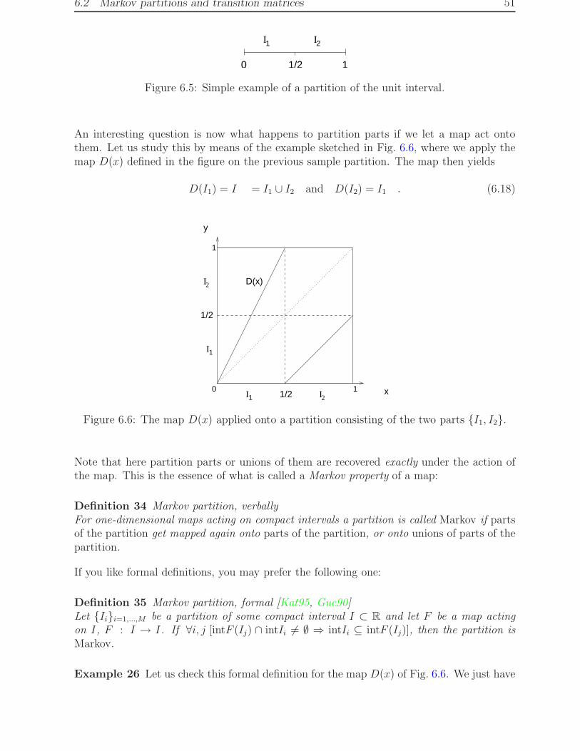
6.2 Markov partitions and transition matrices 51

1/20 1

1 I2I

Figure 6.5: Simple example of a partition of the unit interval.

An interesting question is now what happens to partition parts if we let a map act ontothem. Let us study this by means of the example sketched in Fig. 6.6, where we apply themap D(x) defined in the figure on the previous sample partition. The map then yields

D(I1) = I = I1 ∪ I2 and D(I2) = I1 . (6.18)

I1 I2

I2

I1

10

1

y

x1/2

1/2

D(x)

Figure 6.6: The map D(x) applied onto a partition consisting of the two parts {I1, I2}.

Note that here partition parts or unions of them are recovered exactly under the action ofthe map. This is the essence of what is called a Markov property of a map:

Definition 34 Markov partition, verballyFor one-dimensional maps acting on compact intervals a partition is called Markov if partsof the partition get mapped again onto parts of the partition, or onto unions of parts of thepartition.

If you like formal definitions, you may prefer the following one:

Definition 35 Markov partition, formal [Kat95, Guc90]Let {Ii}i=1,...,M be a partition of some compact interval I ⊂ R and let F be a map actingon I, F : I → I. If ∀i, j [intF (Ij) ∩ intIi 6= ∅ ⇒ intIi ⊆ intF (Ij)], then the partition isMarkov.

Example 26 Let us check this formal definition for the map D(x) of Fig. 6.6. We just have


to verify that the logical implication holds for the four cases

intD(I1) ∩ intI1 6= ∅ ⇒ intI1 ⊆ intD(I1). X



intD(I2) ∩ intI2 = ∅ X (6.19)

It is elucidating to discuss an example of a map with a partition that is not Markov:

Example 27 Let us look at the map E defined in Fig. 6.7.

I2I1

I1

I2

1

y

1/2

0 1 x1/2

E(x)

E(I2)

Figure 6.7: An example of a map E(x) with a partition that is not Markov.

The first branch of the map does not cause any problem, since it is identical with the oneof our previous map D(x). But let us look at the action of the second branch:

intE(I2) ∩ intI1 6= ∅ ⇒ intI1 ⊆ intE(I2). X

intE(I2) ∩ intI2 6= ∅ ⇒ intI2 ⊆ intE(I2). × not true! (6.20)

Consequently, the partition {I1, I2} is not Markov for E(x).

Remark 14

1. Maps for which there exists a Markov partition are often called Markov maps. How-ever, note that sometimes further conditions such as hyperbolicity, smoothness, etc.,are required in the literature.

2. Markov partitions appear to have first been constructed by Sinai in 1968 for the Sinaibilliard. For such higher dimensional systems the principle of Markov partitions is thesame as the one described above, however, the precise definition is technically a bitmore involved than for one-dimensional maps [Kat95, Guc90].

3. Markov partitions are not unique for a given map, see the coursework.


4. Markov partitions are important because they define, loosely speaking, an ‘invariantframe’ according to which the action of a map on statistical ensembles can be described.They enable to map the statistical dynamics of a system onto a Markov process – hencethe name –, which is precisely what we will explore in the following.

As usual, we start with a simple example:

Example 28 The map F shown in Fig. 6.8 is defined on a Markov partition (please convinceyourself that this is the case). Let N i

n be the number of points in partition part i at thenth iteration of this map. Let us start with a uniform distribution of N =

∑

i Nin points on

[0, 1] at time step n = 0. As one can infer from the left part of Fig. 6.8, the dynamics of N in

is then given as follows:

I2I1

I2

I1

N01 N0

2

N12

N11

F(x)

1 x1/20

1

y

1/2

t21

t11 t12

t22

1 x0

1

y

Figure 6.8: Left: A map that enables a matrix representation for the dynamics of a statisticalensemble of points; right: Illustration of where the transition matrix elements come fromfor this map.

N11 =

1

2N1

0 + N20 =

1

2[N1

0 + 2N20 ]

N21 =

1

2N1

0 + 0 · N20 =

1

2N1

0 . (6.21)

This can equivalently be written as(

N11

N21

)

=1

2

(1 21 0

)(N1

0

N20

)

(6.22)

or

Nn+1 =1

2T

FNn , (6.23)

where Nn ∈ R2 is a column vector and TF∈ M2,2 a topological transition matrix (or transfer

matrix) acting on Nn.

Let us focus for a moment on the (topological) structure of the matrix TF. There is a simple

recipe of how to obtain this matrix, as follows:


• Consider a map defined on a Markov partition such as F above.

• Identify the “grid” formed by the Markov partition under iteration of the map withthe rows and columns of the desired matrix T

F, however, by turning the grid “upside

down”.

• Check whether there exist any “links” between partition part i and partition part junder iteration: That is, does the graph of the map intersect the cell labeled by tij?And if so, how many times?

• Count the number of intersections, which yields the value of the matrix element tij .

Applied to the above example of map F , this prescription leads directly to the transitionmatrix T

Fof Eq. (6.22). An alternative representation of a transition matrix for a map is

obtained by using the following definition:

Definition 36 Markov graph [Has03, All97, Rob95]Let F : I → I , I ⊂ R be a map, {Ii} a Markov partition and T

F= ((tij)), i, j ∈ {1, . . . , M}

be the corresponding transition matrix. In a Markov graph tij arrows are drawn from j toi.

Example 29 The Markov graph for the map F of Fig. 6.8 acting on the given Markovpartition is sketched in Fig. 6.9.

1 2

t21

t12

t11

Figure 6.9: Markov graph for the map F on the given Markov partition.

Remark 15

1. What we encounter here is a representation of the action of F in terms of a symbolicdynamics of a map. The above Markov graph defines it with respect to the givenMarkov partition.4

2. Note that our definition is such that tij ∈ N0. In other literature you will usually findthat tij ∈ {0, 1}.5 Why our definition is a bit more convenient for practical purposesyou will see later on.

4Other partitions could be used as well. Symbolic dynamics is a fundamental concept in dynamicalsystems theory, which would deserve much more detailed explanations. However, since this is again a topicof the module on Chaos and Fractals we do not further discuss it in our course and refer to the literatureinstead [Bec93, All97].

5see, e.g., work by Ruelle and Bowen


3. Markov graphs can be constructed without having any transition matrix TF

available.It suffices to just look at how a map F acts onto a Markov partition. If you find itsimpler, you may thus first sketch the Markov graph and then obtain T

Ffrom it.

The following definition now makes mathematically precise what we actually mean with atopological transition matrix:

Definition 37 topological transition matrix (see, e.g., [Guc90])Let {Ii} be a Markov partition and let the map F be invertible on Ii. Then the topologicaltransition matrix T

F= ((tij)) , i, j ∈ {1, . . . , M}, is defined by

tij :=

{1, intIi ⊆ intF (Ij)0 otherwise

. (6.24)

If F is not invertible on Ij, let {Ijk}, k = 1, . . . , L be a refinement of the Markov partitionon Ij such that F is invertible on each Ijk. Then

tij :=

{number of parts Ijk such that intIi ⊆ intF (Ijk)0 otherwise

. (6.25)

Example 30 Let us apply this definition to the map F already studied above. Accordingto Fig. 6.10 F is invertible on I1, and we obtain

I2I1

I2

I1

I22I21

F(x)

1 x1/20

1

y

1/2

Figure 6.10: Construction of a transition matrix for the map F according to Definition 37.

intI1 ⊆ intF (I1) ⇒ t11 = 1

intI2 ⊆ intF (I1) ⇒ t21 = 1 (6.26)

However, F is not invertible on I2, hence we have to use a refinement on which F is invertiblesuch as the one shown in the figure. On this finer partitioning we get

intI1 ⊆ intF (I21) , intI1 ⊆ intF (I22) ⇒ t12 = 2

intI2 ⊆ intF (I21) not true , intI2 ⊆ intF (I22) not true ⇒ t22 = 0 (6.27)


Altogether we thus arrive at

TF

=

(1 21 0

)

, (6.28)

as before.

Let us now reconsider the action of the above transition matrix TF

onto the given Markovpartition. So far you have been provided with several pieces of a puzzle that we can nowput together. Recall Eq. (6.23) for the map F of Fig. 6.10, which read

Nn+1 =1

2T

FNn .

We now divide the whole equation by the product of the total number of points N timesdiam(Ii), where according to Fig. 6.10 diam(Ii) = 1/2. This yields

ρn+1

=1

2T

Fρ

n, (6.29)

where the topological transition matrix TF

acts onto probability density vectors ρn, ρ

n+1,

whose components are constant on the Markov partition parts.So what did we achieve with Eq. (6.29)? Using Markov partitions for a piecewise lin-ear map enabled us to construct the very simple version of the FPE Eq. (6.7), where theFrobenius-Perron operator is represented as a matrix and the probability densities are piece-wise constant step functions in form of vectors. We may expect that such an equation can besolved much more easily than the FPE in its original form. However, before we explore thiswe remark that the above construction can be performed under fairly general conditions:

Proposition 5 Let F : I → I , I ⊆ R be a piecewise linear map with uniformly constantslope |F ′(x)| = const.. If there exists a topological transition matrix T

F, and by restricting

ourselves to probability density vectors ρn

that are constant on Markov partition parts, theFPE of this map can be written as

ρn+1

=1

|F ′(x)| TF

ρn

. (6.30)

The proof of this proposition is a bit too lengthy for our lectures, but we outline the basicidea: First of all, note that for our example of map F considered above the correspondingFrobenius-Perron operator 1/2 T

Factually defines a stochastic matrix, where the sum of all

entries of a column is equal to one,∑M

i=1 tij/2 = 1.6 However, this case is rather special– consider, for example, map G depicted in Fig. 6.11. Based on the information given inthe figure one can show that the constant slope |G′(x)| 6∈ N. It is then easily seen thatthe corresponding matrix T

G/|G′(x)| cannot be a stochastic one, which refers to the typical

situation.Nevertheless, this connection with stochastic matrices points in the right direction: If theconditions of the above proposition are fulfilled there exists a systematic procedure of how to

6We remark that there is no unique definition of a stochastic matrix in the literature: some authorsdefine it as above [Kat95], others require that the sum of all row entries is one, instead of the column entries[Bec93]. Some authors identify a stochastic matrix with a Markov matrix, others distinguish between themdepending on whether the row or the column entries add up to one.


construct the Frobenius-Perron operator in terms of a transition matrix that is generally nota topological but a stochastic one, which acts on probabilities defined on Markov partitionparts, see Section 17.5 of Ref. [Bec93] for details. For uniformly constant slope this stochasticmatrix can be simplified to a topological transition matrix divided by the absolute value ofthe slope, which acts onto probability density vectors as given in the proposition.

I2

I1

I2I10

1/2

G(x)

I3

y1

1x

Figure 6.11: Example of a map G yielding a topological transition matrix that is not directlyrelated to a stochastic one.

Remark 16 For a single vector component Eq. (6.30) reads

ρin+1 = c

M∑

j=1

tij ρjn , (6.31)

where c = const. Note that all matrix elements tij defining the transition from states j attime step n to state i at time step n + 1 are constants. That is, they do not depend onthe history of the process at all previous time steps but are defined with respect to thestates i and j at time steps n + 1 and n only, which is the hallmark of a Markov process.Proposition 5 thus transforms the dynamics generated by the FPE onto a Markov chain[Bec93]. Note, however, that any transition matrix exhibits a specific topological structure,which to some extent characterizes a given map. This structure is encoded in the values ofthe tij ’s, and summing over all these matrix elements can make the corresponding Markovchain arbitrarily complicated.7

If one can transform a Frobenius-Perron operator onto a topological transition matrix,the resulting Frobenius-Perron matrix equation Eq. (6.30) can be used for calculating theinvariant density ρ∗ in form of the following algorithm:

7Interestingly, the topological structure of the transition matrix for a given map can change drasticallyunder tiny variation of control parameters. Such a topological instability of a dynamical system produces asensitivity of the whole dynamics with respect to control parameters [Kla07].


1. For a given map F defined on a Markov partition construct TF.

2. Solve the eigenvalue problem of TF

TFρ

τ= τρ

τ, (6.32)

where τ is an eigenvalue and ρτ

the corresponding eigenvector. If you did this calcu-

lation correctly, you will find that the largest eigenvalue is always equal to |F ′(x)|,8

τmax = |F ′(x)| , (6.33)

with eigenvector ρτmax

.

3. It follows: Chooseρ

n= c ρ

τmax

, (6.34)

where c is a constant. Then according to the Frobenius-Perron matrix equationEq. (6.30)

ρn+1

=c

|F ′|T Fρ

τmax

Eq. (6.32)= c

τmax

|F ′| ρτmax

Eq. (6.33)= cρ

τmax

Eq. (6.34)= ρ

n, (6.35)

from which we can draw the important conclusion that

c ρτmax

= ρ∗ , (6.36)

that is, the largest eigenvector is proportional to the invariant density.

4. It then remains to determine c by normalisation,

m∑

i=1

c ρiτmax

· diam(Ii) = 1 . (6.37)

This recipe of how to calculate invariant densities has a rigorous mathematical underpinning:

Theorem 4 Perron-Frobenius Theorem [Kat95, Rob95]Let T

Fbe such that for a certain power T n

Fall entries are positive.9 Then T

Fhas one

(up to a scalar) eigenvector ρτmax

with positive components and no other eigenvectors with

nonnegative components. The eigenvalue τmax

corresponding to ρτmax

is simple, positive and

greater than the absolute values of all other eigenvalues.

The proof of this important theorem is non-trivial, see the references cited above. If appliedonto stochastic matrices it directly justifies our ‘recipe’ given above, see p.157 of [Kat95].Note that if the conditions of this theorem are fulfilled it guarantees the existence of aunique invariant probability density vector, which gives an answer to the question posed inRemark 13.

Example 31 We now apply the above method for calculating invariant measures of piece-wise linear Markov maps to our previous map F introduced in Example 28:

8This fact is not trivial but a consequence of the following Proposition 4.9A nonnegative matrix that fulfills this property is called eventually positive.


1. The first step in this algorithm we have already performed before, see Examples 28and 30. They yielded the Frobenius-Perron matrix equation

ρn+1

=1

2T

Fρ

n, (6.38)

see Eq. (6.29), where

TF

=

(1 21 0

)

(6.39)

and the probability density vectors are defined by

ρn

=

(ρ1

n

ρ2n

)

∈ R2 , (6.40)

where ρin = const. on the ith Markov partition part.

2. Solve now the eigenvalue problem

TFρ

τ= τρ

τ(6.41)

by calculatingdet(T

F− τI) = 0 , (6.42)

where

I =

(1 00 1

)

(6.43)

is the identity matrix. We find

det

(1 − τ 2

1 −τ

)

= 0, (1 − τ)(−τ) − 2 = 0

− τ + τ 2 − 2 = 0 ⇒ τ =1

2±√

1

4+ 2 =

1

2± 3

2= 2 or − 1 . (6.44)

We see that indeed τmax = |F ′(x)|, as stated to the end of step 2 of our algorithm.

3. We now have to calculate the largest eigenvector by solving the equation(

1 21 0

)(ρ1

τmax

ρ2τmax

)

= 2

(ρ1

τmax

ρ2τmax

)

, (6.45)

which leads to

ρ1τmax

+ 2ρ2τmax

= 2ρ1τmax

ρ1τmax

= 2ρ2τmax

. (6.46)

Assuming that ρ1τmax

= 1 gives

ρ2τmax

=1

2ρ1

τmax=

1

2(6.47)

from which we obtain

ρτmax

=

(112

)

. (6.48)

4. The last step is to calculate ρ∗ by normalisation: It is

ρ∗ = cρτmax

(6.49)

with

1 =

2∑

i=1

ρ∗i · diam(Ii) = c

2∑

i=1

ρiτmax

· diam(Ii) = c3

4(6.50)

from which follows c = 4/3. Our final result thus reads

ρ∗ =

(4323

)

. (6.51)

It is not a bad idea to cross-check whether our solution indeed fulfills the Frobenius-Perronmatrix equation Eq. (6.38),

(4323

)

=1

2

(1 21 0

)(4323

)

=

(23

+ 23

23

)

. X (6.52)

7 Measure-theoretic description ofdynamics

So far we have analyzed the dynamics of statistical ensembles by using probability densities,which represents rather a physicist’s approach towards a probabilistic theory of dynamicalsystems. Mathematicians prefer to deal with measures, which are often more well-behavedthan probability densities.In this chapter we introduce these quantities, learn about basic properties of them andeventually briefly elaborate on some ergodic properties of dynamical systems. The firstsection particularly draws on Ref. [Las94], the second one on Refs. [Dor99, Arn68]. If youhave problems to associate any meaning with measures you may wish to take a look intoRef. [All97].

7.1 Probability measures

Let ρ(x), x ∈ I, be a probability density, see Definition 29. If ρ(x) exists and is integrableon a subinterval A ⊆ I then

µ(A) :=

∫

A

dxρ(x) (7.1)

is the probability of finding a point in A. µ(A) is called a measure of A, in the sense that we‘assign a positive number to the set A’. Let us demonstrate this idea for a simple example:

7.1 Probability measures 61

Example 32 Let I = [0, 1] and A = [0, 12] with ρ(x) = 1 – think, for example, of the

Bernoulli shift. Then

µ(A) =

∫ 1

2

0

dx 1 =1

2(7.2)

is the probability of finding a point in A.

We make this basic idea mathematically precise in terms of two definitions:

Definition 38 [Kat95, Las94]A nonempty countable collection A of subsets of a set I is called a σ-algebra1 if

1. A ∈ A ⇒ I \ A ∈ A complementarity

2. A1, A2, . . . , AN ∈ A ⇒ ⋃

k Ak ∈ A additivity

Example 33 Consider the three intervals I = [0, 1], A1 = [0, 1/2), A2 = [1/2, 1]. IsA = {A1, A2} a σ-algebra? Let us check the two parts of the above definition:

1. A1 ∈ A ⇒ I \ A1 = A2 ∈ A X and vice versa for A2.

2. A1, A2 ∈ A ⇒ A1 ∪ A2 = I ∈ A is not the case.

Even for an amended set {A1, A2, I} the first condition yields I \ I = ∅, which again is notan element of this new set. We thus find that A = {A1, A2, I, ∅} must be a σ-algebra ofI. It is a general feature of σ-algebras that the whole set I as well as the empty set mustalways be elements of the algebra.

Definition 39 [Las94]A function µ : A → R+ ∪∞ defined on a σ-algebra A is called a measure if

1. µ(A) ≥ 0 ∀A ∈ A .

2. µ(∅) = 0.

3. If A1, A2, . . . , An ∈ A and Ai ∩ Aj = ∅ (i 6= j) then

µ(⋃

k

Ak) =∑

k

µ(Ak) σ − additivity . (7.3)

Note the analogy between this definition and Kolmogorov’s axioms of probability theory.

Example 34 Let A = {A1, A2, I, ∅} as before. Let µ(A) be the length of the interval A;for example, if A = [a, b) then µ(A) := b − a. Is this function a measure? Let us check theabove definition step by step:

1. µ(A) ≥ 0 ∀A ∈ A is fulfilled, since a length can never be less than zero.

2. µ(∅) = 0 is also fulfilled.

1The symbol σ refers to the fact that condition 2 applies to a countably infinite number of subintervals,whereas for an ordinary algebra condition 2 applies to any two sets only, i.e. n = 2.

62 7 Measure-theoretic description of dynamics

3. For the third condition we have to check all the different cases:

A1 ∩ A2 = ∅ ⇒ µ(A1 ∪ A2) = µ(I) = 1 = µ(A1) + µ(A2) =1

2+

1

2X

A1 ∩ I 6= ∅ X

A2 ∩ I 6= ∅ X

A1 ∩ ∅ = ∅ ⇒ µ(A1 ∪ ∅) = µ(A1) =1

2= µ(A1) + µ(∅) X , (7.4)

since µ(∅) = 0. The same holds for A2 ∩ ∅ and I ∩ ∅.

We can conclude that µ(A) is a measure. This specific measure, which is defined by thelength of the interval, is called the Lebesgue measure. From now on we will denote it by µL.

These considerations motivate the following definition:

Definition 40 [Kat95] A measure space is a triple (I, A , µ) of a set I, a σ-algebra A ofsubsets of I and a measure µ.

In the following we will always work on measure spaces, mostly without saying it explicitly.For the example above (I, A , µL) defines a measure space. We will furthermore often requirethe following property:

Definition 41 µ is called a probability measure on I if µ(I) = 1.

If we think of µ in terms of Eq. (7.1), this refers to nothing else than normalisation.

Example 35 For any Lebesgue measure µL on I = [0, 1] it is µL(I) = 1, hence it defines aprobability measure. However, note that this does not hold for, say, I = [0, 2].

Remark 17 We emphasize that µL is only one example of a measure. There exist plenty ofother types of measure such as, for example, the Dirac measure discussed in the coursework[Las94].

Let us get back to our motivation Eq. (7.1). Let ρ(x) be a probability density on I ⊆ R andlet A be a σ-algebra on the same interval. Then µ(A) :=

∫

Adxρ(x) , A ∈ A , see Eq. (7.1),

defines a probability measure on I. That this holds true can be verified straightforwardlyby applying Definition 39 and using properties of Riemann integration.Let us now assume that ρ(x) is generated by a map such as, e.g., the Bernoulli shift, seeFig. 7.1. We have the Frobenius-Perron equation (FPE)

ρn+1(x) = PF ρn(x) (7.5)

with Frobenius-Perron operator PF for a map F governing the time evolution of the prob-ability densities ρn(x). The above choice of µ(A) raises the question whether there existsan equation for the evolution of this measure associated with a density that is analogous tothe FPE.In order to answer this question we employ again the principle of conservation of probabilityas for our derivation of the FPE in Section 6.1. With A = F ◦F−1(A) for a one-dimensionalmap F , where F−1(A) defines the preimages of the set A, the number of points xn in F−1(A)


10

1

y

x

B(x)

A

B−1(A)

Figure 7.1: Construction of the analogue of the FPE for the measure obtained by integratinga probability density.

must be equal to the number of points xn+1 in A. This implies that the probability measuresµ(A) =

∫

Adxρ(x) on image and preimages must be the same under iteration,

µn+1(A) = µn(F−1(A)) . (7.6)

See the Bernoulli shift B(X) = 2x mod 1 in Fig. 7.1 for an illustration. We thus arriveat the measure-theoretic version of the FPE Eq. (6.7) [Bec93]. Alternatively, this equationcan be obtained by just integrating the FPE.Recall that the fixed point of the FPE, ρ∗(x) = PF ρ∗(x), yielded the invariant densityof the map F , see Definition 31. This leads to the following analogous defnition for thecorresponding probability measure:

Definition 42 [Bec93]µn+1(A) = µn(A) =: µ∗(A) is called an invariant measure, i.e., the measure does not changewith time.

Hence, for our µ-version of the FPE it must hold that µ∗(A) = µ∗(F−1(A)) [All97]. A mapF that fulfills this property is also sometimes called measure preserving in the mathematicsliterature [Las94].We may now highlight another important property of the probability measure µ(A) obtainedfrom a density in form of the following definition:

Definition 43 absolute continuity [Kat95, Las94, dM93]Consider a measure space (I, A , µL), where I ⊆ R and µL is the Lebesgue measure. Let ρbe a probability density on I. If there exists a continuous

µ(A) :=

∫

A

dxρ(x) ∀A ∈ A , (7.7)

µ is called absolutely continuous with respect to µL.


Remark 18

1. Note that for the Lebesgue measure in the integral one may also write dx = dµL =µL(dx). This more general notation is often used in the mathematics literature.

2. Loosely speaking one may say that a measure is absolutely continuous if it is givenby integrating a density [Kat95, Has03]. However, this only implies continuity for themeasure µ if we specify the space of probability density functions on which we areworking. The function space should then exclude densities ρ that are singular suchas, e.g., the δ−function that we have encountered in Section 3.3, see Eq. (3.15). Thisis also illustrated in the following examples.

3. Rigorously mathematically speaking, the function space on which we should be work-ing here is the space of Lebesgue-integrable functions [Las94]: Let us replace theLebesgue measure µL(dx) by some other measure ν(dx). Then Lp(I, A , ν) , 1 ≤p < ∞ is the family of all possible real-valued measurable functions ρ satisfying∫

ν(dx) |ρ(x)|p < ∞, where this integral should be understood as a Lebesgue in-tegral.2 Note that if ρ ∈ Lp is not Riemann-integrable anymore, it may still beLebesgue-integrable, that is, the above integral may still exist.

4. Some authors define a measure µ to be absolutely continuous with respect to anothermeasure ν if for all measurable sets A ∈ I µ(A) = 0 whenever ν(A) = 0 [dM93, Las94].If ρ ∈ L1 and ν is σ-finite,3 then one can prove that this definition is equivalent toDefinition 43. This is the contents of the Radon-Nikodym Theorem, and ρ = dµ/dν iscalled the Radon-Nikodym derivative of µ with respect to ν [dM93, Las94].

5. If ρ ∈ C0 and bounded it follows from the fundamental theorem of calculus that µ isC1-smooth and dµ/dx = ρ(x).

6. If ρ(x) is continuous except at finitely many points and bounded, then there still existsa measure µ according to Eq. (7.7), however, it is not everywhere C1 anymore.

Let us illustrate the last two points of this remark by two examples:

Example 36

1. Consider the Bernoulli shift B(x) = 2x mod 1 on [0, 1) with ρ∗(x) = 1. It is easy tosee that there exists a differentiable absolutely continuous invariant measure µ∗(x) =∫ x

0dx ρ∗(x) = x.

2. Consider the step function ρ∗(x) sketched in the left part of Fig. 7.2. Integrating overthis function according to µ∗(x) =

∫ x

0dxρ∗(x) yields the graph depicted in the right

part of this figure, which ist still C0 but not differentiable at the points of discontinuityof ρ∗(x).

Definition 44 [Lev94, Las94]If the measure µ defined by Eq. (7.7) is not absolutely continuous, it is called singular.4

2I found the entry on Lebesgue integration in the online Wikipedia quite helpful to get an intuition ofwhat Lebesgue integration is about compared with ordinary Riemann integration.

3A measure is σ-finite if it can be written as the countable union of sets with finite measure.4One may also say that the measure µ defined by Eq. (7.7) decomposes into an absolutely continuous

one µa and a singular one µs, which is the contents of Lebesgue’s decomposition theorem [Las94].


a1

a3

a2

a4

x2 x3x1

x10

ρ

x2 x3x1

x10

µ

1

Figure 7.2: A step function density and the corresponding absolutely continuous probabilitymeasure obtained by integrating the density.

Example 37 For B(x) let ρ∗(x) := 12[δ(x − 1

3) + δ(x− 2

3)] be the invariant density defined

on the period 2 orbit {13, 2

3} only, see the left part of Fig. 7.3. Then µ∗(x) =

∫ x

0dx ρ∗(x),

see the right hand side of this figure, is singular.

x10

1

x10 1/3 2/3 1/3 2/3

1/2

~* ~*ρ µ8

Figure 7.3: A delta function density yields a singular measure via integration.

Definition 45 [All97]A measure µ is called atomic5 if all of the measure is contained in a finite or countablyinfinite set of points.

Example 38 The measure µ∗ of the above example is atomic,6 which in fact is better seenif we look at the measure µ∗(A) on sets A ⊆ [0, 1] rather than µ∗(x).

5In measure theory, an atom is a measurable set which has positive measure and contains no ”smaller”set of positive measure.

6This measure actually represents a linear combination of the Dirac measure as defined on a courseworksheet.


Remark 19 An atomic measure is singular, however, a singular measure is not necessarilyatomic.

For higher-dimensional dynamical systems we commonly have a combination of absolutelycontinuous and singular components of the invariant measure. This leads to another defini-tion, which we first motivate by two examples:

Example 39 [Dor99]

1. The baker map: (see also [Las94])

��

��

��

��

��

��

��

��

��

��

��

��

��

��

��

��

��

��

n=1

n=2 n times

2n layers

n 8

area conservation

x

y

1

1

0

1/2

10 2

1

0 1

Figure 7.4: The two-dimensional area-preserving baker map and its iterative action onto aset of points initially concentrated on the left half of the unit square.

In Fig. 7.4 we geometrically define the famous baker map, a paradigmatic exampleof a two-dimensional area-preserving chaotic dynamical system. This map stretchesthe unit square by a factor of two along the x-axis and squeezes it by a factor of 1/2in the y-direction. The resulting rectangle is cut in the middle, and both halfes areput on top of each other recovering the unit square. If we colour the left half of theunit square (or fill this half uniformly with points while leaving the right half empty,respectively) and iterate this map several times we obtain the layered structure shownin the figure.

Note that the corresponding density ρn(x, y) is uniform in the x direction, whereas itis a step function along y. However, in the limit of n → ∞ the strips become thinner


and thinner such that all points eventually distribute uniformly over the whole square,so there are no “steps” anymore along y. In other words, the invariant density of thebaker map is simply constant everywhere. But if we modify the map a little bit thesituation changes dramatically leading us to our second example.

2. The dissipative baker map:

n=2

��

��

��

��

��

��

��

��

��

��

��

x

y

1

1

0

n=1

n=3 n times

‘Fractal’ structureComplicated

Figure 7.5: The dissipative baker map eventually generates an invariant measure exhibitinga fractal structure in the y direction.

In Fig. 7.5 we introduce a little variant of the previous baker transformation, where westill stretch and squeeze the whole unit square parallel to the x- and to the y-direction,respectively. However, we do this now such that the big left (coloured) rectangle iscompressed into the little rectangle at the bottom of the second unit square, whereasthe little right (empty) rectangle is expanded into the big empty one on top. If werepeat this action, again a layered structure evolves which is similar to the one of theprevious figure. One observes that, as before, the density ρn(x, y) is uniform in thex-direction and that in the limit of n → ∞ the strips piling up along y become thinnerand thinner. However, in contrast to the previous example it can be shown that inthe limit of n → ∞ the invariant density is not uniform anymore on the whole unitsquare. Strictly speaking, in this case an invariant density does not exist anymore,because a fractal structure was generated in the y direction which makes the densityρn(x, y) non-integrable in the limit of n → ∞. However, there still exists an invariantmeasure µ∗(x, y). This measure turns out to be absolutely continuous along x withµ∗(x) ∈ C1 but it is singular along y with µ∗(y) ∈ C0. See [Dor99] for further details.

Definition 46 SRB measure [You02, Eck85, Bal00]An invariant probability measure µ∗ is called an SRB measure7 if it is absolutely continuous

7The acronym SRB holds for the initials of the mathematicians Ya.Sinai, D.Ruelle and R.Bowen whofirst introduced this measure.


along unstable manifolds.

Recall that the unstable manifold W u(p) of a source p of a map can be defined as the set ofinitial conditions whose orbits are repelled from p, see Definition 19. The same applies to pbeing an unstable periodic point.8

Remark 20

1. Some authors define an SRB measure by asking for slightly stronger C1-smoothnessalong unstable manifolds [Eck85].

2. We emphasize that this definition is designed for higher-dimensional dynamical sys-tems, where stable and unstable manifolds typically form complicated structures inphase space. Often the topology of these systems is such that the measure is smoothalong unstable manifolds, whereas it is fractal along stable ones. In this case the to-tal measure is not absolutely continuous, however, it is still SRB. So while absolutecontinuity of the total measure trivially implies that it is SRB, the reverse is not true.

Example 40

1. The Bernoulli shift B(x) = 2x mod 1 is unstable ∀x ∈ [0, 1), since with B′(x) = 2it is everywhere expanding (except at x = 1/2). Hence the whole system lives on anunstable manifold, and µ∗(x) =

∫ x

0dxρ∗(x) =

∫ x

0dx1 = x is an SRB measure.

2. The baker map of Fig. 7.4 has an SRB measure that is smooth along the x axis, whichiidentifies the direction of all unstable manifolds. It is also smooth in the y direction,although this defines the stable manifolds.

3. The dissipative baker map of Fig. 7.5 has an SRB measure that is smooth alongthe unstable manifolds in the x direction. However, it is singular along the stablemanifolds in the y direction.

Remark 21

1. SRB measures are important, because the property of being smooth along at leastone direction in phase space enables one to calculate ensemble averages of (physical)observables, see also the following section.

2. An important question is whether an SRB measure exists for a given dynamical system.These measures are supposed to be quite common, however, their existence is usuallyhard to prove. For so-called Anosov systems an important theorem (sometimes calledthe SRB theorem [Dor99]) ensures the existence of SRB measures [You02]. The abovetwo baker maps are examples of systems which have ‘Anosov-like’ properties [Dor99].

8For further details about the definition of stable and unstable manifolds see [Bec93, Ott93, Eck85].

7.2 Basics of ergodic theory 69

7.2 Basics of ergodic theory

In this section we introduce measure-theoretic properties which form the basis of what iscalled ergodic theory, an important branch of dynamical systems theory. Our presentationparticularly follows [Dor99, Arn68], for further mathematical details see [Kat95].Let as usual F : I → I , xn+1 = F (xn) , n ∈ N0 be a one-dimensional map acting on the setI ⊆ R and µ∗ be a corresponding invariant probability measure. Let us consider a functiong : I → R , g ∈ C0, which we may call an “observable”.

Definition 47 time and ensemble average

g(x) := limn→∞

1

n

n−1∑

k=0

g(xk) , (7.8)

x = x0, is called the time (or Birkhoff) average of g with respect to F .

〈g〉 :=

∫

I

dµ∗g(x) (7.9)

where, if it exists, dµ∗ = ρ∗(x)dx, is called the ensemble (or space) average of g with respectto F . Note that g(x) may depend on x, whereas 〈g〉 does not.

Example 41 In Definition 25 we have introduced the local Ljapunov exponent of a mapF . If we choose g(x) = ln |F ′(x)| as the observable in Eq. (7.8), we find that

λt(x) := ln |F ′(x)| = limn→∞

1

n

n−1∑

k=0

ln |F ′(xk)| , (7.10)

so calculating the local Ljapunov exponent actually means taking a time average along atrajectory. If we choose the same observable for the ensemble average Eq. (7.9) we obtain

λe := 〈ln |F ′(x)|〉 :=

∫

I

dxρ∗(x) ln |F ′(x)| . (7.11)

Let us check these two definitions for the Bernoulli shift B(x) = 2x mod 1, where B′(x) = 2for almost every x: We have that

λt(x) =1

n

n−1∑

k=0

ln 2 = ln 2 (7.12)

for almost every x ∈ [0, 1) and that

λe =

∫ 1

0

dxρ∗(x) ln 2 =

∫ 1

0

dx1 · ln 2 = ln 2 . (7.13)

In other words, time and ensemble average are the same for almost every x,

λt(x) = λe = ln 2 . (7.14)


gi��

i

I

Figure 7.6: Uniform partition of the interval I ⊆ R and a local average gi defined on theith partition part of an observable g(x).

In the following we will show that this result is not a coincidence. We do so in two steps:

Step 1: Let us define a uniform partition on the interval I, see Fig. 7.6, with a totalnumber of N partition parts, where the ith partition part is defined by the subintervalIi := [xi, xi+1]. Take a long trajectory {x0, x1, . . . , xn−1} generated by the map F and let ni

with∑N

i=1 ni = n be the number of occurrences when the trajectory is in partition part i.Let gi be the local average of g(x) with respect to the ith partition part,

gi :=1

ni

∑

k

g(xk) ∀xk ∈ Ii . (7.15)

Then

g(x) =1

n

n−1∑

k=0

g(xk) =1

n

N∑

i=1

nigi =N∑

i=1

ni

ngi . (7.16)

There is now a famous hypothesis relating the number of occurrences ni in the bin i to theinvariant probability measure µ∗

i of the region i. Before we can state it we need the followingdefinition:

Definition 48 almost everywhere [Kat95, Ott93]A property is said to hold µ-almost everywhere if the set of elements for which the propertydoes not hold is of measure zero with respect to a given measure µ. In this case one alsosays that the property holds for a typical element.

Hypothesis 1 Boltzmann’s ergodic hypothesis (1871) [Dor99, Tod92]The trajectory of a typical point in I spends equal time in regions of equal measure.

If this hypothesis applies we have that

ni

n=

µ∗i

µ∗(I)= µ∗

i , (7.17)

which together with Eq. (7.16) implies that

g(x) =N∑

i=1

µ∗i gi →

∫

I

dµ∗g(x) = 〈g〉 (n, N → ∞) . (7.18)

Step 1 summarizes Boltzmann’s intuitive approach to relate time and ensemble averages ofobservables. His hypothesis forms the rigorous foundation of the whole theory of statistical


mechanics [Tod92]. Step 2 now makes his idea mathematically precise by starting with animportant theorem:

Theorem 5 Birkhoff’s ergodic theorem (1931) [Dor99, Kat95, Arn68, Tod92]If there exists an invariant probability measure µ∗(I) with

∫

Idµ∗|g(x)| < ∞9 then for µ∗-

almost every x ∈ I there exists g(x).

For a proof see [Kat95]. Note that this theorem only ensures the existence of the timeaverage. It does not say anything about uniqueness, that is, g(x) might be different fordifferent initial conditions x ∈ I. However, this is clarified by the following definition:

Definition 49 ergodicity [Arn68, Dor99]A dynamical system is called ergodic if

g(x) = 〈g〉 (7.19)

µ∗-almost everywhere.

This implies that g(x) does not depend on x anymore. That the time average is constant issometimes also taken as a definition of ergodicity in the literature [Dor99, Bec93]. In fact,there is even a third definition, which is based on the following definition:

Definition 50 decomposability [Arn68]Assume I is the disjoint union of two sets I1, I2 of positive measure, each of which is in-variant under the map F : F (I1) = I1, F (I2) = I2. Such a system is called decomposable.

With this definition we have the following proposition:

Proposition 6 A map F is ergodic if and only if F on I is indecomposable.

The proof of this proposition is not hard [Dor99, Arn68]. In turn, sometimes this statementis used to define ergodicity [Kat95]. The equivalence between time and ensemble averagestated by Definition 49 then follows as a proposition. Let us discuss these notions by twoexamples:

Example 42

1. The “double tent map” shown in Fig. 7.7 is certainly decomposable. According toProposition 6 it is therefore not ergodic.

2. The Bernoulli shift B(x) is indecomposable and hence ergodic. However, a proof ofthis property is a bit cumbersome and goes along the lines as the one of ergodicity forthe baker map [Dor99].

3. The rotation on the unit circle Rα : S1 → S1 , Rα(θ) := θ + 2πα , α ∈ R as defined onone of the coursework sheets is non-ergodic if α is rational and ergodic if α is irrational.See [Arn68, Dor99, Tod92] for proofs, the one for ergodicity is a bit more elaborate.

9Strictly speaking this means that we require g to be Lebesgue-integrabel, g ∈ L1, see Remark 18.


I1 I2

I2

I1

10

1

y

x1/2

1/2

Figure 7.7: An example of a map that is decomposable and hence not ergodic.

Remark 22 You may have noticed that the properties of a map being topologically tran-sitive and being ergodic are of a very similar nature. However, note that ergodicity requiresus to use a measure, whereas topological transitivity works without a measure. In fact, fora continuous map it can be shown under fairly general conditions that ergodicity impliestopological transitivity, whereas the reverse does not hold [Kat95, Rob95].10

Let us now get back to the Ljapunov exponent studied in Example 41. For time averageλt(x) and ensemble average λe we have found that

λt(x) = λe = const. (7.20)

for the Bernoulli shift. From Definition 49 we have learned that this result must holdwhenever a map F is ergodic. However, this means that in case of ergodicity the Ljapunovexponent λ becomes a global quantity characterising a given map F for a typical pointx, irrespective of what value we choose for the initial condition, λt(x) = λe = λ. Thisobservation very much facilitates the calculation of λ, as is demonstrated by the followingexample:

Example 43 Let us reconsider our specific map F which has already been introducedpreviously, see Example 28. For convenience we display it again in Fig. 7.8.

In Example 31 the invariant density of this map was calculated to

ρ∗(x) =

{43, 0 ≤ x < 1

223, 1

2≤ x < 1

, (7.21)

see Eq. (6.51). This motivates us to calculate the Ljapunov exponent of this map by using

10For example, the reverse implication does not hold for the Pomeau-Manneville map.


F(x)

1 x1/20

1

y

1/2

Figure 7.8: A simple map that we have seen before, here used in order to demonstrate thecalculation of Ljapunov exponents via ensemble averages.

the ensemble average Eq. (7.11). We obtain

λe =

∫ 1

0

dxρ∗(x) ln |F ′(x)| = ln 2

(∫ 1

2

0

dx4

3+

∫ 1

1

2

dx2

3

)

= ln 2

(4

3· 1

2+

2

3· 1

2

)

= ln 2 .

(7.22)Actually, this result trivally follows from the fact that the slope of this map is uniform andthat the probability density normalises to one. However, the calculation demonstrates howthe definition of λ by ensemble averages could be used in case the slope and the invariantdensity are more complicated functions. By assuming that the map F is ergodic (which hereis the case), we can conclude that this result for λ represents the value for typical points inthe domain of F .

We conclude this section by using the concept of ergodicity for a further characterisation ofinvariant measures:

Definition 51 physical measure [You02]Let F : I → I , I ⊆ R, be a map and µ∗ be an invariant probability measure of this map. µ∗

is called a physical (or natural) measure if for an observable g : I → R, g ∈ C0 the map isergodic, that is, g(x) = 〈g〉 for µ∗-almost every x ∈ I.

Remark 23

1. Note that by restricting ourselves to typical points and considering measures that aredefined with respect to integrating probability densities we sort out periodic orbits,which are all of Lebesgue measure zero.

2. It is important to observe that a measure being SRB neither implies that it is physical,nor is the reverse true. For both directions one can construct counterexamples [You02,Bal00, Eck85]. For example, our double tent map considered above has an SRB


measure but not an ergodic one. On the other hand, the map C(x) = x/2 contractingonto a fixed point has trivially an ergodic measure on the attracting fixed point which,however, is not SRB.

3. Some authors define an SRB measure via ergodicity, so the definitions of SRB andphysical measure are not unique in the literature.

4. An alternative definition of a physical measure first suggested by Kolmogorov yieldsthe physical measure as the measure that emerges in the zero-noise limit of a dynamicalsystem under random perturbations [Eck85].

5. The SRB theorem mentioned before proves that for Anosov systems the SRB measureis equal to the physical one [You02], which identifies an important class of dynamicalsystems where both measures are identical.

6. You may wonder why physical measures are important at all. This is for the followingreason: Pick your favourite (physical) system such as, for example, the driven pen-dulum that we have encountered at the very beginning of these lectures. You maywish to characterize such a system in a statistical sense by calculating your favouriteobservable in terms of time or ensemble averages. You would hope that your averagesexist (i.e., that your computations converge to specific values in the limit of long timesor of large ensembles of points), and also that your results do not depend on the ini-tial conditions you choose. In mathematical terms, you would thus expect that thereexists a “nice” measure which guarantees that your averages exist and are the same.If your system exhibits a physical measure, it is the one you will typically “see” bymeasuring your observable. And being SRB guarantees that you can calculate yourobservables by projection along the unstable manifolds.

If you are further interested, I would highly recommend that you make yourself familiarwith what is called mixing in ergodic theory, see, e.g., [Arn68, Dor99].

Bibliography

[All97] K.T. Alligood, T.S. Sauer and J.A. Yorke, Chaos - An introduction to dynamicalsystems. (Springer, New York, 1997).

[Arn68] V.I. Arnold and A. Avez, Ergodic problems of classical mechanics. (W.A. Benjamin,New York, 1968).

[Bal00] V. Baladi, Positive Transfer Operators and Decay of Correlations, volume 16 ofAdvanced Series in Nonlinear Dynamics. (World Scientific, Singapore, 2000).

[Ban92] J. Banks, J. Brooks, G. Cairns, G. Davis and P. Stacey, On Devaney’s definitionof chaos. Amer. Math. Monthly 99, 332–334 (1992).

[Bec93] C. Beck and F. Schlogl, Thermodynamics of Chaotic Systems, volume 4 of Cam-bridge nonlinear science series. (Cambridge University Press, Cambridge, 1993).

[Dev89] R.L. Devaney, An introduction to chaotic dynamical systems. (Addison-Wesley,Reading, second edition, 1989).

[dM93] W. de Melo and S. van Strien, One-dimensional dynamics, volume 25 of Ergebnisseder Mathematik und ihrer Grenzgebiete, 3.Folge. (Springer, Berlin, 1993).

[Dor99] J.R. Dorfman, An introduction to chaos in nonequilibrium statistical mechanics.(Cambridge University Press, Cambridge, 1999).

[Eck85] J.-P. Eckmann and D. Ruelle, Ergodic theory of chaos and strange attractors. Rev.Mod. Phys. 57, 617–656 (1985).

[Elm98] F.-J. Elmer. The Pendulum Lab. University of Basel, 1998. Online simulation athttp://monet.unibas.ch/∼elmer/pendulum.

[Fot05] A. Fotiou, Deterministic chaos. Master’s Thesis, School of Mathematical Sci-ences, Queen Mary, University of London, 2005. see http://www.mpipks-dresden.mpg.de/∼rklages/people/msc fotiou.pdf.

[Gas98] P. Gaspard, Chaos, scattering, and statistical mechanics. (Cambridge UniversityPress, Cambridge, 1998).

[Gla93] E. Glasner and B. Weiss, Sensitive dependence on initial conditions. Nonlinearity6, 1067–1075 (1993).

[Gle96] J. Gleick, Chaos: Making a New Science. (Vintage, 1996).

76 Bibliography

[Guc79] J. Guckenheimer, Sensitive dependence to initial conditions for one dimensionalmaps. Comm. Math. Phys. 70, 133–160 (1979).

[Guc90] J. Guckenheimer and P. Holmes, Nonlinear oscillations, dynamical systems, andbifurcations of vector fields, volume 42 of Applied mathematical sciences. (Springer,Berlin, 3rd edition, 1990).

[Has03] B. Hasselblatt and A. Katok, A first course in dynamics. (Cambridge UniversityPress, 2003).

[Kat95] A. Katok and B. Hasselblatt, Introduction to the modern theory of dynamical sys-tems, volume 54 of Encyclopedia of Mathematics and its Applications. (CambridgeUniversity Press, Cambridge, 1995).

[Kla07] R. Klages, Microscopic chaos, fractals and transport in nonequilibrium statisticalmechanics, volume 24 of Advanced Series in Nonlinear Dynamics. (World Scientific,Singapore, 2007).

[Las94] A. Lasota and M.C. Mackay, Chaos, Fractals, and Noise. (Springer-Verlag, 1994).

[Lev94] R.W. Leven, B.-P. Koch and B. Pompe, Chaos in dissipativen Systemen. (AkademieVerlag, Berlin, second edition, 1994).

[Miy03] T. Miyasaka and T. Harayama. Corrugated floor simulation, 2003. Simulationcourtesy of Dr. Takahisa Harayama and Dr. Tomohiro Miyasaka, ATR labs, Kyoto,Japan.

[Ott93] E. Ott, Chaos in Dynamical Systems. (Cambridge University Press, Cambridge,1993).

[Rob95] C. Robinson, Dynamical Systems. (CRC Press, London, 1995).

[Smi07] L. Smith, Chaos - A very short introduction. (Oxford University Press, Oxford,2007).

[Str94] S. H. Strogatz, Nonlinear Dynamics and Chaos: With Applications to Physics,Biology, Chemistry, and Engineering. Studies in nonlinearity. (Addison Wesley,Reading, MA, 1994).

[Tel06] T. Tel and M. Gruiz, Chaotic Dynamics. (Cambridge University Press, Cambridge,2006).

[Tod92] M. Toda, R. Kubo and N. Saito, Statistical Physics, volume 1 of Solid State Sci-ences. (Springer, Berlin, 2nd edition, 1992).

[Wig92] S. Wiggins, Chaotic transport in dynamical systems, volume 2 of InterdisciplinaryApplied Mathematics. (Springer, New York, 1992).

[You02] L.-S. Young, What are SRB measures, and which dynamical systems have them?J. Stat. Phys. 108, 733–754 (2002).

Introduction to Dynamical Systems - QMUL Mathsklages/mas424/lnotes_ds2007f.pdf · Introduction to...

Documents

Transcript of Introduction to Dynamical Systems - QMUL Mathsklages/mas424/lnotes_ds2007f.pdf · Introduction to...