Introduction to Dynamic Light Scattering for Particle Size ......images for RM 8011 Technique Size...

© 2016 HORIBA, Ltd. All rights reserved. 1© 2016 HORIBA, Ltd. All rights reserved. 1

Introduction to Dynamic Light Scattering for Particle Size

Determination

www.horiba.com/us/particle

Jeffrey Bodycomb, Ph.D.

© 2016 HORIBA, Ltd. All rights reserved. 3

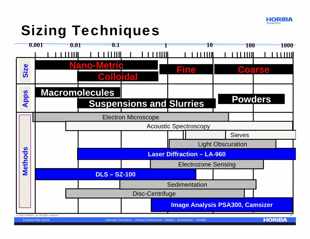
0.01 0.1 1 10 100 10000.001

Colloidal

Suspensions and Slurries

DLS – SZ-100

Electron Microscope

Powders

Fine Coarse

Image Analysis PSA300, Camsizer

Laser Diffraction – LA-960

Acoustic Spectroscopy

Electrozone Sensing

Disc-Centrifuge

Light Obscuration

Macromolecules

Nano-Metric

Met

hods

App

sA

pps

Size

Size

Sedimentation

Sieves

Sizing Techniques


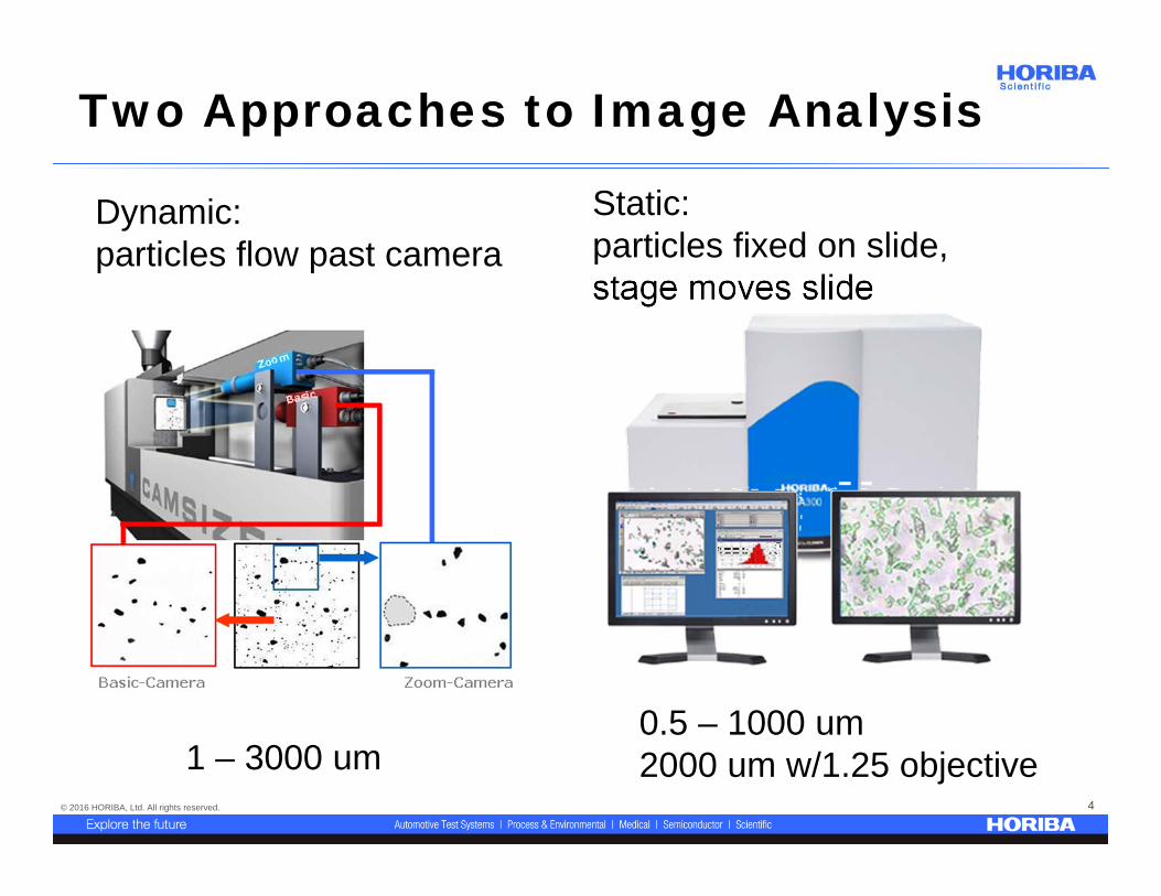
Dynamic:particles flow past camera

Static:particles fixed on slide,stage moves slide

1 – 3000 um0.5 – 1000 um2000 um w/1.25 objective

Two Approaches to Image Analysis


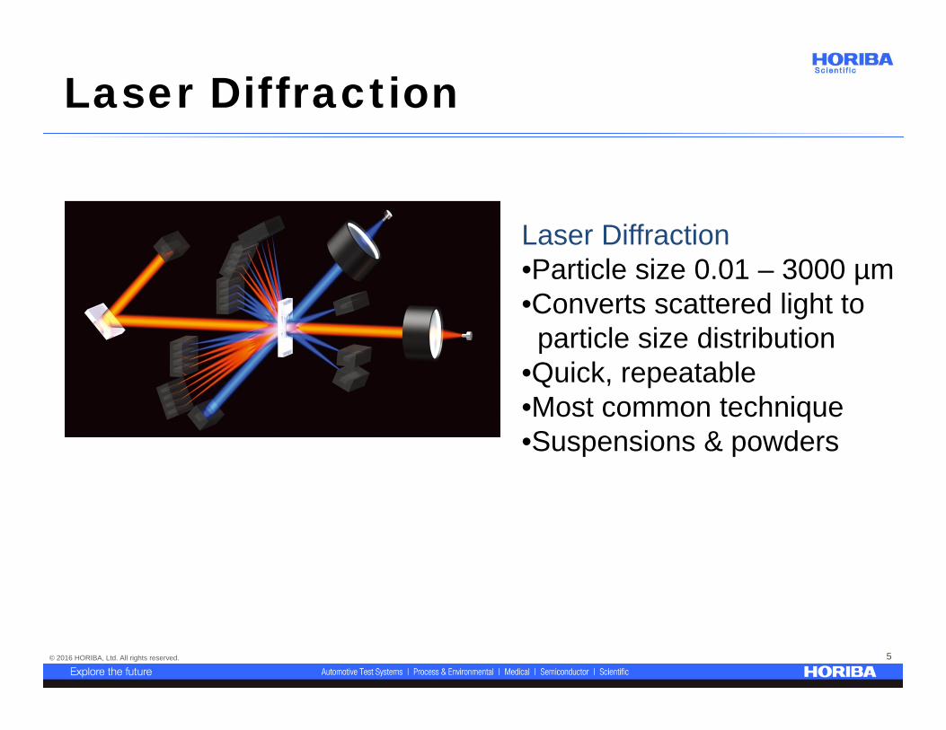
Laser Diffraction•Particle size 0.01 – 3000 µm•Converts scattered light to particle size distribution

•Quick, repeatable•Most common technique•Suspensions & powders

Laser Diffraction


Laser Diffraction

q(%

)

Diameter(µm)

0

14

2

4

6

8

10

12

10.00 3000100.0 10000

100

10

20

30

40

50

60

70

80

90

Silica~ 30 nm

Coffee Results0.3 – 1 mm

Suspension Powders


What is Dynamic Light Scattering?

• Dynamic light scattering refers to measurement and interpretation of light scattering data on a microsecond time scale.

• Dynamic light scattering can be used to determine – Particle/molecular size– Size distribution– Relaxations in complex fluids


Other Light Scattering Techniques

• Static Light Scattering: over a duration of ~1 second. Used for determining particle size (diameters greater than 10 nm), polymer molecular weight, 2nd virialcoefficient, Rg.

• Electrophoretic Light Scattering: use Doppler shift in scattered light to probe motion of particles due to an applied electric field. Used for determining electrophoretic mobility, zeta potential.


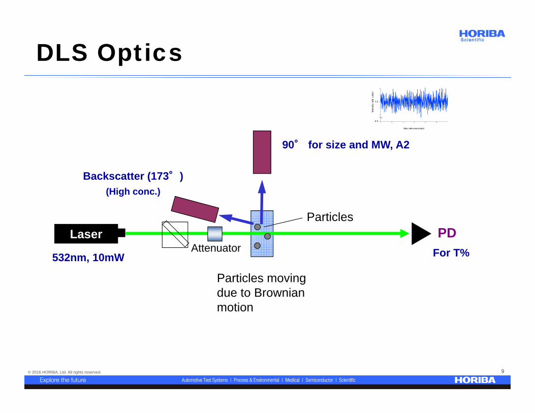
Particles

Backscatter (173°)(High conc.)

90° for size and MW, A2

Laser PDFor T%532nm, 10mW

Attenuator

Particles movingdue to Brownianmotion

DLS Optics


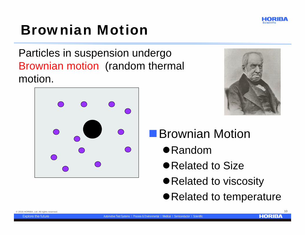
Particles in suspension undergo Brownian motion (random thermal motion.

Brownian MotionRandomRelated to SizeRelated to viscosityRelated to temperature

Brownian Motion


DLS signal

• Random motion of particles leads to random fluctuations in signal (due to changing constructive/destructive interference of scattered light.


Correlation Function

• Random fluctuations are interpreted in terms of the autocorrelation function (ACF), C().

)2exp(1)( C

)()(

)()()( 0

tItI

dttItIC

T


Gamma to Size

2sin4 nq

m

Bh DT

TkD)(3

2qDm decay constantDm diffusion coefficientq scattering vectorn refractive index wavelength scattering angleDh hydrodynamic diameter viscositykB Boltzman’s constant

Note effect of temperature!


What is Hydrodynamic Size?

• DLS gives the diameter of a sphere that moves (diffuses) the same way as your sample.

Dh DhDh


Hydrodynamic Size• The instrument reports the size of sphere

that moves (diffuses) like your particle.• This size will include any stabilizers bound

to the molecule (even if they are not seen by TEM).

SEM (above) and TEM (below) images for RM 8011

Technique Size nmAtomic Force Microscopy 8.5 ± 0.3Scanning Electron Microscopy 9.9 ± 0.1Transmission Electron Microscopy 8.9 ± 0.1Dynamic Light Scattering 13.5 ± 0.1

Gold Colloids


Nanogold Data

Z-avg. Diameter, nm

Run 1 50.5

Run 2 51.1

Run 3 49.2

Run 4 51.5

Run 5 49.7

Run 6 50.9

Avg. 50.5

St. Dev.

0.9

COV 1.7 %


Nanogold Data

Z-avg. Diameter, nm

Run 1 10.5Run 2 10.6Run 3 10.2Run 4 10.5Run 5 10.3Avg. 10.4St. Dev.

0.2

COV 1.9 %

Z-avg. Diameter, nm

Avg. 50.5St. Dev. 0.9

COV 1.7 %


Lab to Lab comparison

Mean determined Z-average size

(nm)

COV (%)

Dynamic Light Scattering with

SZ-100, laboratory 1

34.4 0.7

Dynamic Light Scattering with

SZ-100, laboratory 2

34.6 0.3

Colloidal Silica


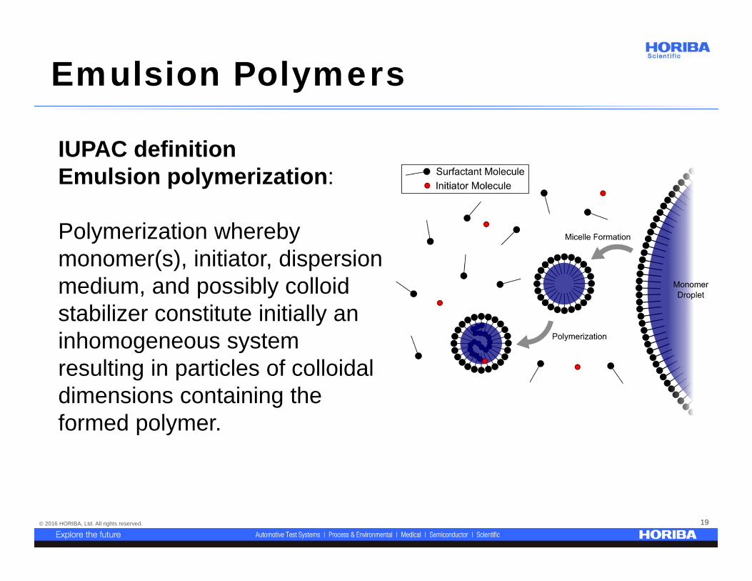
Emulsion Polymers

IUPAC definitionEmulsion polymerization:

Polymerization whereby monomer(s), initiator, dispersionmedium, and possibly colloid stabilizer constitute initially an inhomogeneous systemresulting in particles of colloidal dimensions containing the formed polymer.


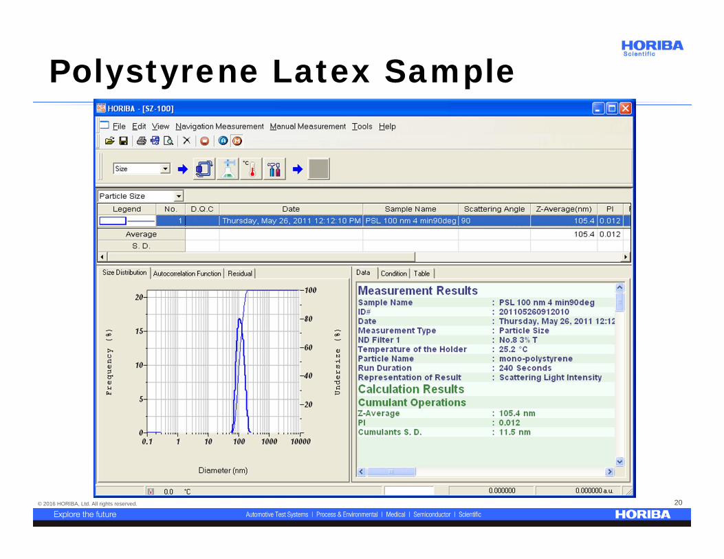
Polystyrene Latex Sample


Polydisperse Sample CumulantsFor a mixture of sizes, the autocorrelation function can be interpreted in terms of cumulants. This is the most robust method of analyzing DLS data.

m

Bhz DT

TkD)(3,

22

!22exp1)( C

2qDm

22

sityPolydisper

“z-average size”

)2exp(1)( C


SiO2

Run Z-average Diameter (nm)

Polydispersity Index

1 473.2 0.1272 479.5 0.0663 478.8 0.0774 487.7 0.039Avg. 479.8 0.077


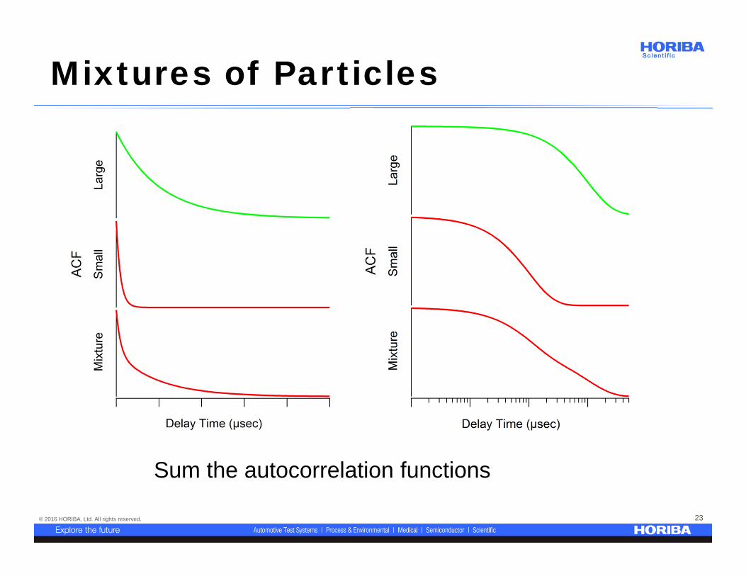
Mixtures of Particles

Sum the autocorrelation functions


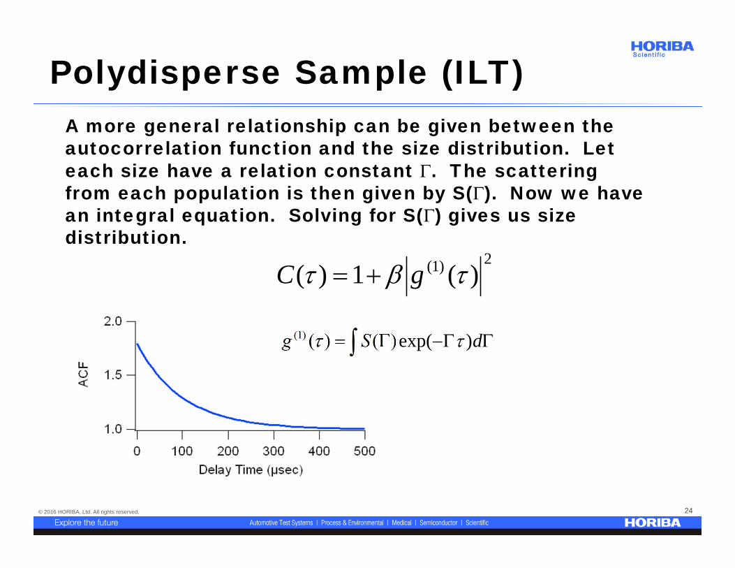
Polydisperse Sample (ILT)A more general relationship can be given between the autocorrelation function and the size distribution. Let each size have a relation constant . The scattering from each population is then given by S(). Now we have an integral equation. Solving for S() gives us size distribution.

dSg )exp()()()1(

2)1( )(1)( gC


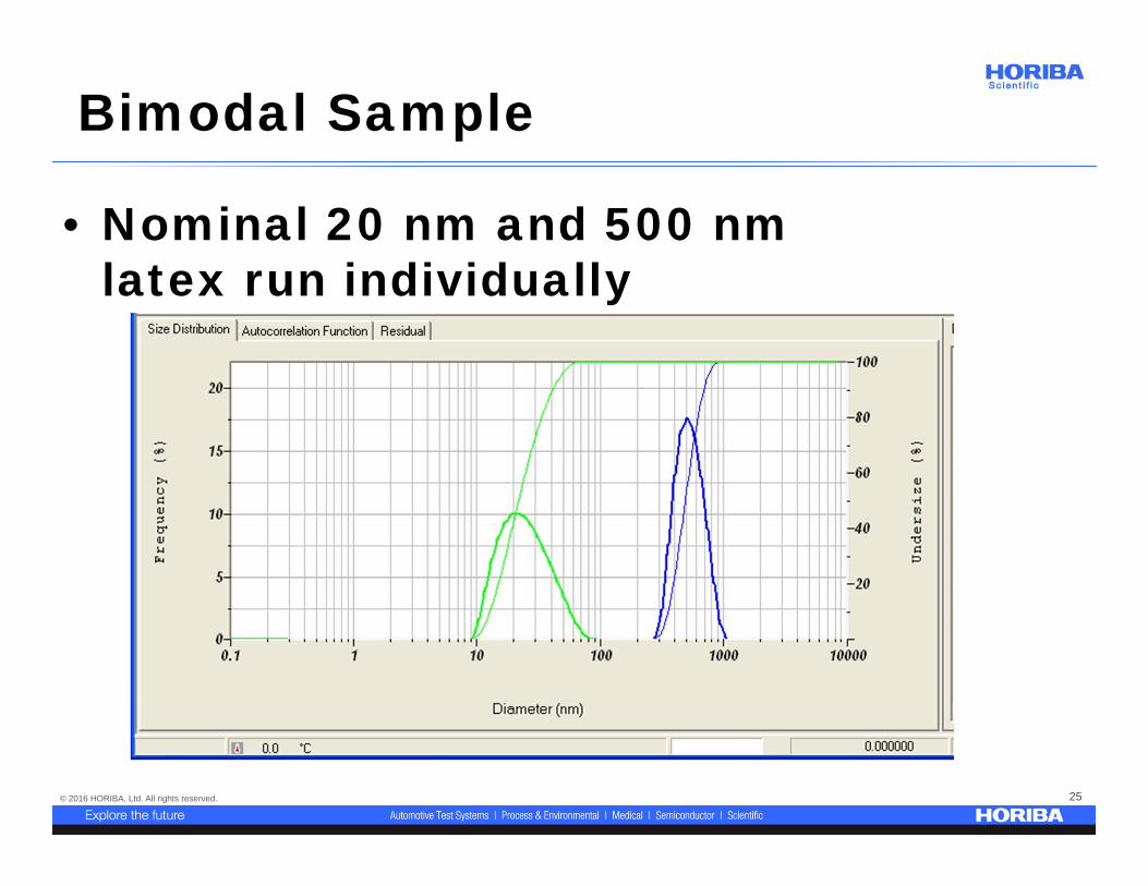
Bimodal Sample

• Nominal 20 nm and 500 nm latex run individually


Bimodal Sample

• Mixed sample (in black)


Dust

• Dust: large, rare particles in the sample

• Generally not really part of the sample

• Since they are rare cannot get good statistics


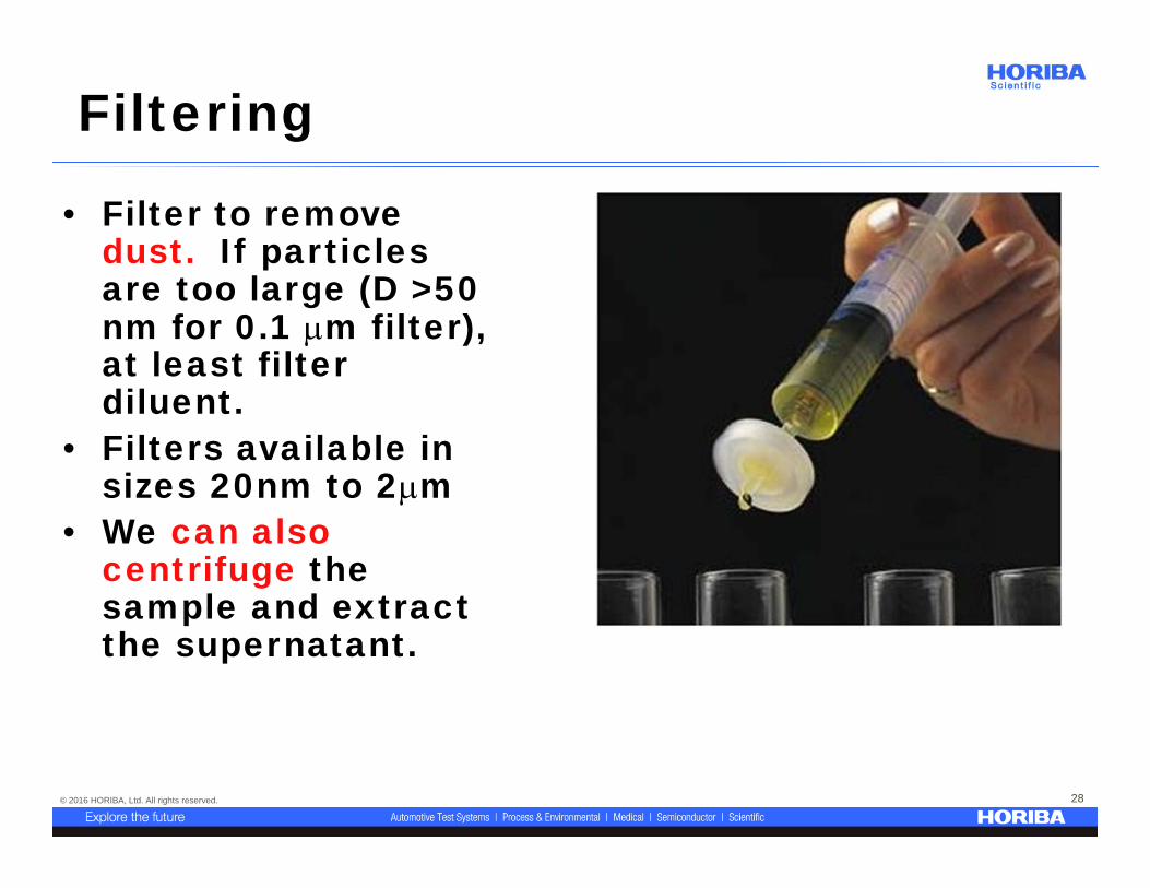
Filtering

• Filter to removedust. If particles are too large (D >50 nm for 0.1 m filter), at least filter diluent.

• Filters available in sizes 20nm to 2m

• We can also centrifuge the sample and extract the supernatant.


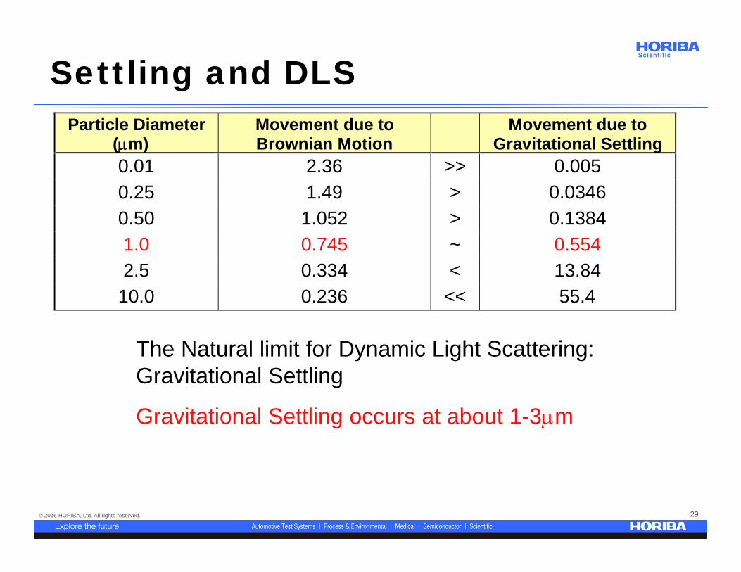
The Natural limit for Dynamic Light Scattering: Gravitational Settling

Gravitational Settling occurs at about 1-3m

Particle Diameter(m)

Movement due toBrownian Motion

Movement due toGravitational Settling

0.01 2.36 >> 0.0050.25 1.49 > 0.03460.50 1.052 > 0.13841.0 0.745 ~ 0.5542.5 0.334 < 13.84

10.0 0.236 << 55.4

Settling and DLS


Why DLS?

• Non-invasive measurement• Requires only small quantities of

sample• Good for detecting trace amounts

of aggregate• Good technique for macro-

molecular sizing


Nanoparticle Analyzer

• Single compact unit that performs size, zeta potential, and molecular weight measurements.


Q&A

Ask a question at [email protected]

Keep reading the monthly HORIBA Particle e-mail newsletter!

Visit the Download Center to find the video and slides from this webinar.

Jeff Bodycomb, Ph.D. P: 800-446-7422E: [email protected]

Introduction to Dynamic Light Scattering for Particle Size ......images for RM 8011 Technique Size...

Documents

Transcript of Introduction to Dynamic Light Scattering for Particle Size ......images for RM 8011 Technique Size...