Introduction to Differential...
62
- Introduction to Differential Equations w ith the systematic study of differential equations, the calculus of functions of a single variable reaches a state of completion. Modeling by differential equations greatly expands the list of possible applications. The list continues to grow as we discover more differential equation models in old and in new areas of application. The use of differential equations makes available to us the full power of the calculus. When explicit solutions to differential equations are available, they can be used to predict a variety of phenomena. Whether explicit solutions are available or not, we can usually compute useful and very accurate approximate numerical solutions. The use of modem computer technology makes possible the visualization of the results. Furthermore, we continue to discover ways to analyze solutions without knowing the solutions explicitly. The subject of differential equations is solving problems and making predic- tions. In this book, we will exhibit many examples of this-in physics, chemistry, and biology, and also in such areas as personal finance and forensics. This is the process of mathematical modeling. If it were not true that differential equations were so useful, we would not be studying them, so we will spend a lot of time on the modeling process and with specific models. In the first section of this chapter we will present some examples of the use of differential equations. The study of differential equations, and their application, uses the derivative and the integral, the concepts that make up the calculus. We will review these ideas starting in Sections 1.2 and 1.3. A . 1
Transcript of Introduction to Differential...
-
Introduction to Differential Equations w ith the systematic study of differential equations, the calculus of functions of a single variable reaches a state of completion. Modeling by differential equations greatly expands the list of possible applications. The list continues to grow as we discover more differential equation models in old and in new areas of application. The use of differential equations makes available to us the full power of the calculus.
When explicit solutions to differential equations are available, they can be used to predict a variety of phenomena. Whether explicit solutions are available or not, we can usually compute useful and very accurate approximate numerical solutions. The use of modem computer technology makes possible the visualization of the results. Furthermore, we continue to discover ways to analyze solutions without knowing the solutions explicitly.
The subject of differential equations is solving problems and making predic- tions. In this book, we will exhibit many examples of this-in physics, chemistry, and biology, and also in such areas as personal finance and forensics. This is the process of mathematical modeling. If it were not true that differential equations were so useful, we would not be studying them, so we will spend a lot of time on the modeling process and with specific models. In the first section of this chapter we will present some examples of the use of differential equations.
The study of differential equations, and their application, uses the derivative and the integral, the concepts that make up the calculus. We will review these ideas starting in Sections 1.2 and 1.3.
A . 1
I oduction t o Differential Equations
la1 Equation Models To start our study of differential equations, we will give a number of examples. This list is meant to be indicative of the many applications of the topic. It is far from being exhaustive. In each case, our discussion will be brief. Most of the examples will be discussed later in the book in greater detail. This section should be considered as advertising for what will be done in the rest of the book.
The theme that you will see in the examples is that in every case we compute the rate of change of a variable in two different ways. First there is the mathematical way. In mathematics, the rate at which a quantity changes is the derivative of that quantity. This is the same for each example. The second way of computing the rate of change comes from the application itself and is different from one application to another. When these two ways of expressing the rate of change are equated, we get a differential equation, the subject we will be studying.
Mechanics Isaac Newton was responsible for a large number of discoveries in physics and math- ematics, but perhaps the three most important are the following:
The systeinatic development of the calculus. Newton's achievement was the realization and utilization of the fact that integration and differentiation are operations inverse to each other. The discovery of the laws of mechanics. Principal among these was Newton's second law, which says that force is equal to the rate of change of momentum with respect to time. Momentum is defined to be the product of mass and velocity, or mu. Thus the force is equal to the derivative of the momentum. If the mass is constant,
d d v -mu = /?I-- = m a , r l t d t
where a is the acceleration. Newton's second law says that the rate of change of momentum is equal to the force F. Expressing the equality of these two ways of loolung at the rate of change, we get the equation
F = ma, (1.1)
the standard expression for Newton's second law. The discovery of the universal law of gravitation. This law says that any body with mass M attracts any other body with mass m directly toward the mass M , with a magnitude proportional to the product of the two masses and inversely proportional to the square of the distance separating them. This means that there is a constant G, which is universal, such that the magnitude of the force is
G M m
r2 '
where r is the distance between the two bodies.
1.1 Differential Equation Models 3
All of these discoveries were made in the period betweell 1665 and 167 1. The discoveries were presented originally in Newton's E-'liilo.so~~lzic~c NCI~LII.(I~~.V Pt-illci/)i(l Mutherncztic~r, better known as Principia M~~thrwzt~tira, published in 1687.
Newton's de\relopment of the calculus is what makes the theory and use of differential equations possible. His laws of mechanics create a templ;lte for a nod el for motion in allnost complete generality. It is necessary in each case to figure out what forces are acting on a body. His law of gravitation does just that in one very important case.
The simplest example is the motion of a ball thrown into the air near the surface of the earth. If .r measures the distance the ball is above the earth, then the velocity and acceleration of the ball are
d.r . du d 2 ~ x LI = - and a = - = -
dt d t dt" Since the ball is assumed to move only a short distance in comparison to the radius of the earth. the force given by (1.2) may be assumed to be constant. Notice that nz, the mass of the ball, occurs in (1.2). We can write the force as F = -mg, where g = G M / ~ ~ and r is the radiu5 of the earth. The constant g is called the earth's acceleration due to gravity. The minus sign reflects the fact that the displacement x is measured positively above the surface of the earth, and the force of gravity tends to decrease x. Newton's second law, (1. l), becomes
d v d'x - ntg = ma = nl- = m-.
rl t dt2 The masses cancel, and we get the differential equatinn
d 2 x p = -g . (1.3)
which is our mathematical model for the rrotion of the ball. The equation in (1.3) is called a differential equation because it involves an
unknown function .r(t) and at least one of its derivatives. In this case the highest derivative occurring is the second order, so this is called a differential equation of second order.
A more interesting example of the application of Newton's ideas has to do with planetary motion. For this case, we will assume that the sun with mass M is tixed and put the origin of our coordinate system at the center of'the sun. We will denote by x ( t ) the vector that gives the location of a planet relative to the sun. The vector x(t) has three components. Its derivative is
d x v(t) = -,
d t which is the vector valued velocity of the planet. For this example, Newton's second law and his law of gravitation become
d 2 x GMnl x m- = dt2 /xI2 1x1'
This system of three second-order differential equations is Newton's model of planetary motion. Newton solved these and verified that the three laws observed by Kepler follow from his model.
loduction t o Differential Equations
Population models Consider a population P ( t ) that is varying with time.' A mathematician will say that the rate at which the population is changing with respect to time is given by the derivative
d P d t
However, the population biologist will say that the rate of change is roughly propor- tional to the population. This means that there is a constant r , called the reproductive rate, such that the rate of change is equal to r P . Putting together the ideas of the mathematician and the biologist, we get the equation
This is an equation for the function P ( t ) . It involves both P and its derivative, so it is a differential equation. It is not difficult to show by direct substitution into (1 .4 ) that the exponential function
P ( t ) = poerf
is a solution. Thus, assuming that the reproductive rate r is positive, our population will grow exponentially.
If at this point you go back to the biologist he or she will undoubtedly say that the reproductive rate is not really a constant. While that assumption works for small populations, over the long term you have to take into account the fact that resources of food and space are limited. When you do, a better model for the the reproductive rate is the function r ( l - P I K ) , and then the rate at which the population changes is better modeled by r (1 - PI K ) P . Here both r and K are constants.
When we equate our two ideas about the rate at which the population changes, we get the equation
This differential equation for the function P ( t ) is called the logistic equation. It is much harder to solve than (1 .4) , but it does a creditable job of predicting how single populations grow in isolated circumstances.
Pollution Consider a lake that has a volume of V = 100 km3. It is fed by an input river, and there is another river which is fed by the lake at a rate that keeps the volume of the lake constant. The flow of the input river varies with the season, and assuming that t = 0 corresponds to January 1 of the first year of the study, the input rate is
Notice that we are measuring time in years. Thus the maximum flow into the lake occurs when t = 114, or at the beginning of April.
'For the time being, the population can be anything-humans, paramecia, butterflies, etc. We will be more careful later.
1.1 Differential Equation Models 5
In addition, there is a factory on the lake that introduces a pollutant into the lake at the rate of 2 kmVyear. Let x ( t ) denote the total amount of pollution in the lake at time t . If we make the assumption that the pollutant is rapidly mixed throughout the lake, then we can show that x ( t ) satisfies the differential equation
This equation can be solved and we can then answer questions about how dan- gerous the pollution problem really is. For example, if we know that a concentration of less than 2% is safe, will there there be a problem? The solution will tell us.
The assumption that the pollutant is rapidly mixed into the lake is not very realistic. We know that this does not happen, especially in this situation, where there is a flow of water through the lake. This assumption can be removed, but to do so, we need to allow the concentration of the pollutant to vary with position in the lake as well as with time. Thus the concentration is a function c ( t , x , y , z ) , where (x, y , z ) represents a position in the three-dimensional lake. Instead of assuming perfect mixing, we will assume that the pollutant diffuses through water at a certain rate.
Once again we can construct a mathematical model. Again it will be a differ- ential equation, but now it will involve partial derivatives with respect to the spatial coordinates x , y, and z , as well as the time t .
Personal finance How much does a person need to save during his or her work life in order to be sure of a retirement without money worries? How much is it necessary to save each year in order to accumulate these assets? Suppose one's salary increases over time. What percent of one's salary should be saved to reach one's retirement goal?
All of these questions, and many more like them, can be modeled using dif- ferential equations. Then, assuming particular values for important parameters like return on investment and rate of increase of one's salary, answers can be found.
Other examples We have given four examples. We could have given a hundred more. We could talk about electrical circuits, the behavior of musical instruments, the shortest paths on a complicated-looking surface, finding a family of curves that are orthogonal to a given family, discovering how two coexisting species interact, and many others.
All of these examples use ordinary differential equations. The applications of partial differential equations go much farther. We can include electricity and mag- netism; quantum chromodynamics, which unifies electricity and magnetism with the weak and strong nuclear forces; the flow of heat; oscillations of many kinds, such as vibrating strings; the fair pricing of stock options; and many more.
The use of differential equations provides a way to reduce many areas of appli- cation to mathematical analysis. In this book, we will learn how to do the modeling and how to use the models after we make them.
oduction t o Differential Equations
................ EXERCISES The phrase "y is proportional to x" implies that .y is related to x via the equation y = k x , where k is a constant. In a similar manner, "y is proportional to the square of x" implies y = kx', " y is proportional to the product of ,T and ,-" implies y = kx,- , and " y is inversely proportional to the cube of x" implies y = k / x ! For example, when Newton proposed that the force of attraction of one body on another is proportional to the product of the masses and inversely proportional to the square of the distance between them, we can immediately write
GM1n F = - ,
r2
where G is the constant of proportionality, usually known as the universal gravita- tional constant. In Exercises 1-10, use these ideas to model each application with a differential equation. All rates are assumed to be with respect to time.
1. The rate of growth of bacteria in a petri dish is proportional to the number of bacteria in the dish.
2. The rate of growth of a population of field mice is inversely proportional to the square root of the population.
3. A certain area can sustain a maximum population of 100 ferrets. The rate of growth of a population of ferrets in this area is proportional to the product of the population and the difference between the actual population and the maximum sustainable population.
4. The rate of decay of a given radioactive substance is proportional to the amount of substance remaining.
5. The rate of decay of a certain substance is inversely proportional to the amount of substance remaining.
6. A potato that has been cooking for some time is removed from a heated oven. The room temperature of the kitchen is 65°F. The rate at which the potato cools is proportional to the difference between the room temperature and the temperature of the potato.
7. A thermometer is placed in a glass of ice water and allowed to cool for an ex- tended period of time. The themlometer is removed from the ice water and placed in a room having temperature 77°F. The rate at which the thermometer warms is proportional to the difference in the room temperature and the tem- perature of the thermometer.
8. A particle moves along the x-axis, its position from the origin at time t given by x ( t ) . A single force acts on the particle that is proportional to but opposite the object's displacement. Use Newton's law to derive a differential equation for the object's motion.
9. Use Newton's law to develop the equation of motion for the particle in Exercise 8 if the force is proportional to but opposite the square of the particle's velocity.
10. Use Newton's law to develop the equation of motion for the particle in Exercise 8 if the force is inversely proportional to but opposite the square of the particle's displacement from the origin.
1.2 The Derivative 7
11. The voltage drop across an inductor is proportional to the rate at which the current is changing with respect to time.
1.2 The Derivative Before reading this section, ask yourself, "What is the derivative?'Several answers may come to mind, but remember your first answer.
Chances are very good that your answer was one of the following five:
1. The rate of change of a function
Table 1 A table of 2. The slope of the tangent line to the graph of a function
derivatives 3. The best linear approximation of a function
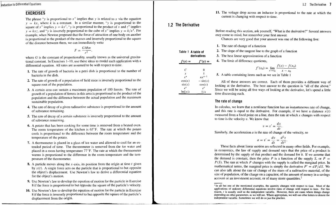
f (x) = f'(r) = 4. The limit of difference quotients,
f ' (xo) = lim f ( - r ) - f (xo) C 0 x-'xo x - XO
X 1 5. A table containing items such as we see in Table 1 xn nxn-'
cos(x) - sin(x) All of these answers are correct. Each of them provides a different way of sin(x) Cos(x) looking at the derivative. The best answer to the question is "all of the above."
ex ex Since we will be using all five ways of looking at the derivative, let's spend a little In(l1-I) 'IX time discussing each.
The rate of change In calculus, we learn that a nonlinear function has an instantaneous rate of change, and this rate is equal to the derivative. For example, if we have a distance x ( t ) measured from a fixed point on a line, then the rate at which x changes with respect to time is the velocity v . We know that
f d x v = x =-. d t
Similarly, the acceleration a is the rate of change of the velocity, so
d v d ' ~ a = v = - = - d t dt2 '
These facts about linear motion are reflected in many other fields. For example, in economics, the law of supply and demand says that the price of a product is determined by the supply of that product and the demand for it. If we assume that the demand is constant, then the price P is a function of the supply S, or P = P ( S ) . The rate at which P changes with the supply is called the marginal price. In mathematical terms, the marginal price is simply the derivative P' = d P / d S . We can also talk about the rate of change of the mass of a radioactive material, of the size of population, of the charge on a capacitor, of the amount of money in a savings account or an investment account, or of many more quantities.'
'In all but one of the mentioned examples, the quantity changes with respect to time. Most of the applications of ordinary differential equations involve rates of change with respect to time. For this reason, t is usually used as the independent variable. However, there are cases where things change depending on other parameters, as we will see. Where appropriate, we will use other letters to denote the independent variable. Sometimes we will do so just for practice.
lodUCtion to Differential Equations
We will see all of these examples and more in this book. The point is that when any quantity changes, the rate at which it changes is the derivative of that quantity. It is this fact that starts the modeling process and makes the study of differential equations so useful. For this reason we will refer to the statement that the derivative is the rate of change as the modeling definition of the derivative.
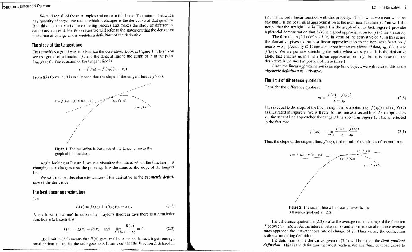
The slope of the tangent line This provides a good way to visualize the derivative. Look at Figure 1. There you see the graph of a function f , and the tangent line to the graph of f at the point (xo, f (x")). The equation of the tangent line is
From this formula, it is easily seen that the slope of the tangent line is f ' (xo).
Figure 1 The derivative is the slope of the tangent line to the graph of the function.
Again looking at Figure 1, we can visualize the rate at which the function f is changing as x changes near the point xo. It is the same as the slope of the tangent line.
We will refer to this characterization of the derivative as the geometric defini- tion of the derivative.
The best linear approximation Let
L is a linear (or affine) function of .r. Taylor's theorem says there is a remainder function R(x) , such that
R ( x ) f (x) = L ( x ) + R ( x ) and lirn - = 0.
++xo X - X o
The limit in (2.2) means that R ( x ) gets small as x -+ xo. In fact, it gets enough smaller than x - xo that the ratio goes to 0. It turns out that the function L defined in
1.2 The Derivative 9
(2. I) is the only linear function with this property. This is what we mean when we say that L is the best linear approximation to the nonlinear function f . You will also notice that the straight line in Figure 1 is the graph of L. In fact, Figure 1 provides a pictorial demonstration that L ( x ) is a good approximation for f ( x ) for x near .yo.
The formula in (2.1) defines L(.r) in terms of the derivative of f . In this sense, the derivative gives us the best linear approximation to the nonlinear function f near .x = xo. [Actually (2.1) contains three important pieces of data, xo, f (x") , and f l ( . ro). We are perhaps stretching the point when we say that it is the derivative alone that enables us to find a linear approximation to f , but it is clear that the derivative is the most important of these three.]
Since the linear approximation is an algebraic object, we will refer to this as the algebraic definition of derivative.
The limit of difference quotients Consider the difference quotient
This is equal to the slope of the line through the two points (xo, f (xo)) and ( x , f ( x ) ) as illustrated in Figure 2. We will refer to this line as a secant line. As .r approaches xo, the secant line approaches the tangent line shown in Figure 1. This is reflected in the fact that
f '(xo) = lim f ( x ) - f (xo) "+To X - . Y O
Thus the slope of the tangent line, f ' ( xo ) , is the limit of the slopes of secant lines.
Figure 2 The secant line with slope rn given by the difference quotient in (2.3).
The difference quotient in (2.3) is also the average rate of change of the function f between xo and x . As the interval between xo and x is made smaller, these average rates approach the instantaneous rate of change of f . Thus we see the connection with our modeling definition.
The definition of the derivative given in (2.4) will be called the limit quotient definition. This is the definition that most mathematicians think of when asked to -

p d u c t i o n to Differential Equations
define the derivative. However, as we will see, it is also very useful, even when attempting to find mathematical models.
The table of formulas By memorizing a table of derivatives and a few formulas (especially the chain rule), we can learn the skill of differentiation. It isn't hard to be confident that you can compute the derivative of any given function. This skill is important. However, it is clear that this formulaic de$nition of derivative is quite different from those given previously.
A complete understanding of the formulaic definition is important, but it does not provide any information about the other definitions we have examined. There- fore, it helps us neither to apply the derivative in modeling nature nor to understand its properties. For that reason, the formulaic definition is incomplete. This is not true of the other definitions. Starting with one of them, it is possible to construct a table that will give us the formulaic finesse we need. However, admittedly that is a big task. That was what was done (or should have been done) in your first calculus course.
To sum up, we have examined five definitions of the derivative. Each of these emphasizes a different aspect or property of the derivative. All of them are impor- tant. We will see this as we progress through the study of differential equations. If your answer to the question at the beginning of the section was any of these five, your answer is correct. However, a complete understanding of the derivative requires the understanding of all five definitions.
Even if your answer was not on the list of five, it may be correct. The famous mathematician William Thurston once compiled a list of over 40 "definitions" of the derivative. Of course many of these appear only in more advanced parts of math- ematics, but the point is made that the derivative appears in many ways in mathemat- ics and in its applications. It is one of the most fundamental ideas in mathematics and in its application to science and technology.
We can start once more by aslung the question, "What is the integral?" This time our list of possible answers is not so long.
1. The area under the graph of a function
2. The antiderivative
3. A table containing items such as we see in Table 1
Let's look at each of them briefly.
The area under the graph The first answer emphasizes the definite integral. The integral
1.3 Integration 11
Table 1 A table of integrals
f ( x ) = I f (x) dx = f ( x ) = l f ( x ) d x =
is interpreted as the area under the graph of the function f , between x = a and x = b. It represents the area of the shaded region in Figure I.
This is the most fundamental definition of the integral. The integral was in- vented to solve the problem of finding the area of regions that are not simple rect- angles or circles. Despite its origin as a method to use in this one application, it has found numerous other applications.
Figure 1 The area of the shaded region is the integral ;n (3.1).
The antiderivative This answer emphasizes the indefinite integral. In fact, the phrase indejinite inte- gral is a synonym for antiderivative. The definition is summed up in the following equivalence. If the function g is continuous, then
f ' = g if and only if 1 g(x) d x = f ( x ) + C . (3 .2)
htroduction to Differential Equations
In (3.2), C refers to the arbitrary constant of integration. Thus the process of indefi- nite integration involves finding antiderivatives. Given a function g , we want to find a function f such that f ' = g.
The connection between the definite and the indefinite integral is found in the fundamental theorem of calculus. This says that if f ' = g , then
J h g ( x ) d x = f ( h ) - f ( a ) .
The table of formulas This formulaic approach to the integral has the same features and failures as the formulaic approach to the derivative. It leads to the handy skill of integration, but it does not lead to any deep understanding of the integral.
All of these approaches to the integral are important. It is very important to understand the first two and how they are connected by the fundamental theorem. However, for the elementary part of the study of ordinary differential equations, it is really the second and third approaches that are most important. In other words, it is important to be able to find antiderivatives.
Solution by integration The solution of an important class of differential equations amounts to finding an- tiderivatives. A first-order differential equation can be written as
Y' = f ( t , y ) , (3.3)
where the right-hand side is a function of the independent variable t and the un- known function y. Suppose that the right-hand side is a function only of r and does not depend on y. Then equation (3.3) becomes
y' = f ( t ) .
1 Comparing this with (3.2), we see immediately that the solution is
y ( t ) = f ( t ) d t
Let's look at an example.
L E 3 . 5 + Solve the differential equation y1 = COS t .
h According to (3.4), the solution is
) ( I ) = / COS(~) d t = sin t + C. J
where C is an arbitrary constant. That's pretty easy. It is just the process of integra- tion. It's old hat to you by now. Solving the more general equation in (3.3) is not so easy, as we will see.
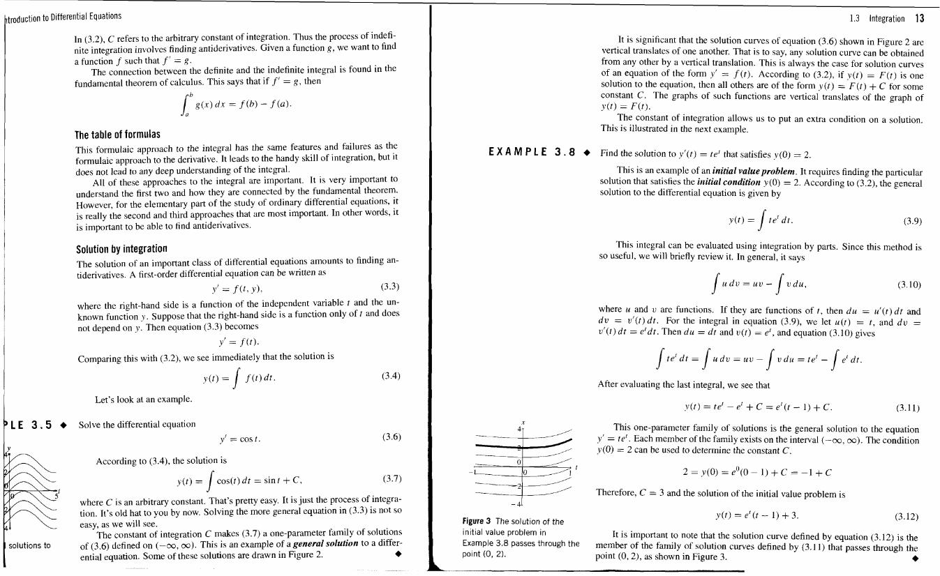
The constant of integration C makes (3.7) a one-parameter family of solutions solutions to of (3.6) defined on (-oo, w). This is an example of a general solution to a differ-
ential equation. Some of these solutions are drawn in Figure 2. +
1.3 Integration 13
It is significant that the solution curves of equation (3.6) shown in Figure 2 are vertical translates of one another. That is to say, any solution curve can be obtained from any other by a vertical translation. This is always the case for solution curves of an equation of the form y' = f ( t ) . According to (3.2), if y ( t ) = F ( r ) is one solution to the equation, then all others are of the form y ( t ) = F ( t ) + C for some constant C. The graphs of such functions are vertical translates of the graph of y ( t ) = F ( t ) .
The constant of integration allows us to put an extra condition on a solution. This is illustrated in the next example.
E X A M P L E 3 . 8 + Find the solution to y l ( t ) = te' that satisfies y(0) = 2.
This is an example of an initial valueproblem. It requires finding the particular solution that satisfies the itzitial condition y(0) = 2. According to (3.2), the general solution to the differential equation is given by
y(r) = S tet d t . (3.9)
This integral can be evaluated using integration by parts. Since this method is so useful, we will briefly review it. In general, it says
S u d v = u v - 1 v d u ,
where u and v are functions. If they are functions of t , then d u = u l ( t ) d t and d v = v l ( t ) d t . For the integral in equation (3.9), we let u ( r ) = t , and d v = v l ( t ) d t = etdt . Then d u = dt and v(r) = el, and equation (3.10) gives
After evaluating the last integral, we see that
This one-parameter family of solutions is the general solution to the equation -+z y' = tet . Each member of the family exists on the interval (-oo, oo). The condition y(0) = 2 can be used to determine the constant C.
t 2 = y(0) = eO(O- 1) + C = -1 + C
% Therefore, C = 3 and the solution of the initial value problem is -
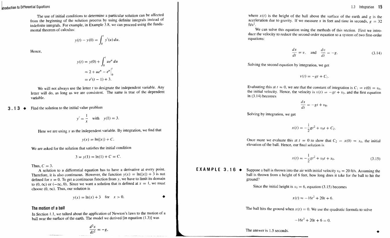
y ( t ) = et( t - 1 ) + 3. (3.12) Figure 3 The solution of the initial value problem in It is important to note that the solution curve defined by equation (3.12) is the
1 Example 3.8 Passes through the member of the family of solution curves defined by (3.1 1 ) that passes through the I
point (0, 2). point ( 0 , 2 ) , as shown in Figure 3.
l tmdudion to Differential Equations
The use of initial conditions to determine a particular solution can be affected from the beginning of the solution process by using definite integrals instead of indefinite integrals. For example, in Example 3.8, we can proceed using the funda- mental theorem of calculus:
Hence,
We will not always use the letter t to designate the independent variable. Any letter will do, as long as we are consistent. The same is true of the dependent variable.
3 . 1 3 Find the solution to the initial value problem
1 y' = - with y (1 ) = 3 .
X
Here we are using x as the independent variable. By integration, we find that
We are asked for the solution that satisfies the initial condition
Thus, C = 3. A solution to a differential equation has to have a derivative at every point.
Therefore, it is also continuous. However, the function y ( x ) = ln((x1) + 3 is not defined for x = 0 . To get a continuous function from y , we have to limit its domain to ( 0 , oo) or ( - o o , 0). Since we want a solution that is defined at x = 1 , we must choose ( 0 , oo ) . Thus, our solution is
y ( x ) = In(x) + 3 for x > 0 .
The motion of a ball In Section 1 . 1 , we talked about the application of Newton's laws to the motion of a ball near the surface of the earth. The model we derived [in equation (1.3)] was
1.3 Integration 15
where x ( t ) is the height of the ball above the surface of the earth and g is the acceleration due to gravity. If we measure x in feet and time in seconds, g = 32 ft/s2.
We can solve this equation using the methods of this section. First we intro- duce the velocity to reduce the second-order equation to a system of two first-order equations:
d x - d v - = u . and - - -g. (3 .14 ) d t dr
Solving the second equation by integration, we get
Evaluating this at t = 0, we see that the constant of integration is CI = v ( 0 ) = UI),
the initial velocity. Hence, the velocity is v ( t ) = -gt + v", and the first equation in (3 .14) becomes
Solving by integration, we get
Once more we evaluate this at t = 0 to show that C2 = ~ ( 0 ) = xO, the initial elevation of the ball. Hence, our final solution is
1 ~ ( t ) = --gt2 + Uot + Xo.
2 (3 .15)
E X A M P E 3 . 1 6 Suppose a ball is thrown into the air with initial velocity vg = 20 ft/s. Assuming the ball is thrown from a height of 6 feet, how long does it take for the ball to hit the ground?
Since the initial height is xo = 6, equation (3 .15 ) becomes
The ball hits the ground when x ( t ) = 0 . We use the quadratic formula to solve
The answer is 1.5 seconds.
ltlOdUction to Differential Equations
EXERCISES
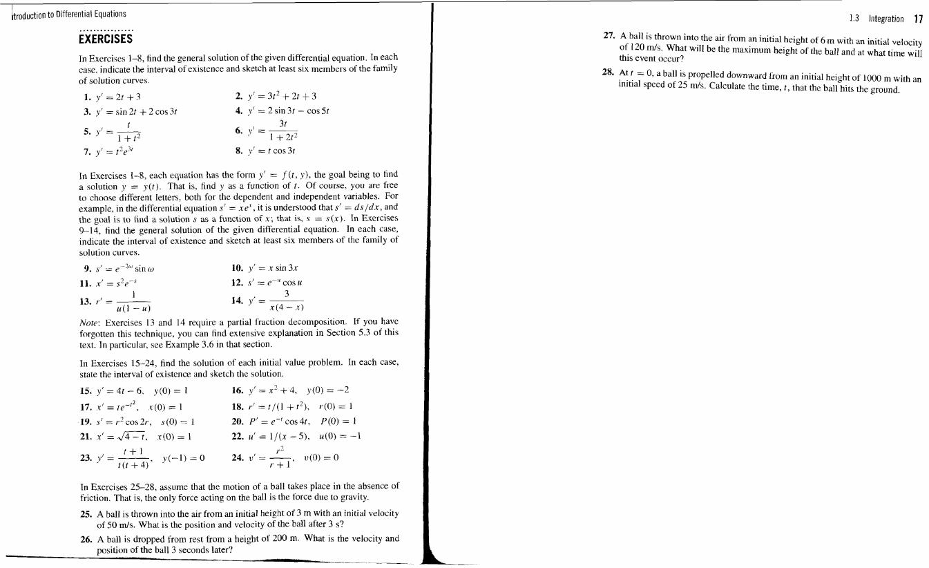
In Exercises 1-8, find the general solution of the given differential equation. In each case, indicate the interval of existence and sketch at least six members of the family of solution curves.
1. y' = 2t + 3 2. y' = 3t2 + 2t + 3
3. y' = sin 2t + 2 cos 3t 4. j' = 2sin3r - cos5t
In Exercises 1-8, each equation has the form y' = f (t, y), the goal being to find a solution y = y(t). That is, find y as a function of t. Of course, you are free to choose different letters. both for the dependent and independent variables. For example, in the differential equation s' = xel , it is understood that s' = dsldx, and the goal is to find a solution s as a function of x; that is, s = s(x). In Exercises 9-14, find the general solution of the given differential equation. In each case, indicate the interval of existence and sketch at least six members of the family of solution curves.
9. s' = e-2W sin w 10. y' = I sin 3x
11. x' = s2p+ 12. s' = e-" cos u
Note: Exercises 13 and 14 require a partial fraction decomposition. If you have forgotten this technique, you can find extensive explanation in Section 5.3 of this text. In particular, see Example 3.6 in that section.
In Exercises 15-24, find the solution of each initial value problem. In each case, state the interval of existence and sketch the solution.
12 17. x' = re- , ~ ( 0 ) = 1 18. r' = t / ( l + t 2 ) , r(0) = 1
19. s' = r2 cos 2r, s (0) = 1 20. P 1 = e - ' c o s ~ ~ , P ( O ) = l
21. .r' = w, x ( 0 ) = 1 22. u ' = l / (x - 3 , u(0) = -1
Tn Exercises 25-28, assume that the motion of a ball takes place in the absence of friction. That is, the only force acting on the ball is the force due to gravity.
25. A ball is thrown into the air from an initial height of 3 m with an initial velocity of 50 mls. What is the position and velocity of the ball after 3 s?
26. A ball is dropped from rest from a height of 200 m. What is the velocity and position of the ball 3 seconds later?
-
1.3 Integration 17 27. A ball is thrown into the air from an initial height of 6 m with an initial velocity
of 120 m/s. What will be the maximum height of the ball and at what time will this event occur?
28. At r = 0, a ball is propelled downward from an initial height of 1000 m with an initial speed of 25 rnls. Calculate the time, t, that the ball hits the ground.
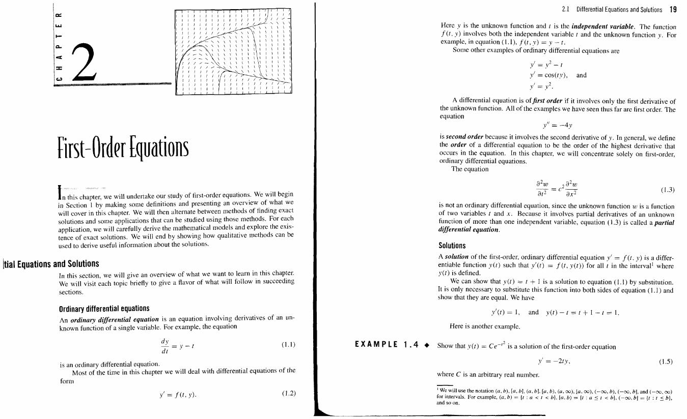
First-Order Equations I n this chapter. we will undertake our study of first-order equations. We will begin in Section 1 by making some definitions and presenting an overview of what we will cover in this chapter. We will then alternate between methods of finding exact solutions and some applications that can be studied using those methods. For each application, we will carefully derive the mathematical models and explore the exis- tence of exact solutions. We will end by showing how qualitative methods can be used to derive useful information about the solutions.
/tial Equations and Solutions In this section, we will give an overview of what we want to learn in this chapter. We will visit each topic briefly to give a flavor of what will follow in succeeding sections.
Ordinary differential equations An ordinary differential equation is an equation involving derivatives of an un- known function of a single variable. For example, the equation
is an ordinary differential equation. Most of the time in this chapter we will deal with differential equations of the
form
I 2.1 Differential Equations and Solutions 19
Here y is the unknown function and t is the independent variable. The function f ( t , y) involves both the independent variable t and the unknown function y. For example, in equation ( l . l ) , f ( t , y) = y - t.
Some other examples of ordinary differential equations are
2 y = y - 1
yf=cos( ty) , and 2 y = y .
A differential equation is offirst order if it involves only the first derivative of the unknown function. All of the examples we have seen thus far are first order. The equation
Y'/ = -4y
is second order because it involves the second derivative of y. In general, we define the order of a differential equation to be the order of the highest derivative that occurs in the equation. In this chapter, we will concentrate solely on first-order, ordinary differential equations.
The equation
is not an ordinary differential equation, since the unknown function w is a function of two variables t and s. Because it involves partial derivatives of an unknown function of more than one independent variable, equation (1.3) is called a partial differential equation.
Solutions A solution of the first-order, ordinary differential equation y' = f (t, p) is a differ- entiable function y(t) such that yl(t) = f (t, y(t)) for all t in the interval' where y(t) is defined.
We can show that y(t) = t + I is a solution to equation (1.1) by substitution. It is only necessary to substitute this function into both sides of equation (1.1) and show that they are equal. We have
y l ( t ) = l , and y ( t ) - t = t + l - t = l .
Here is another example.
E X A M P L E 1 . 4 Show that y(t) = cc t2 is a solution of the first-order equation
I where C is an arbitrary real number. - ' We will use the notation (a, b), [a, bl, (a, bl. [a, b), (a, oo), [a , co), (-co, b), (-w, b ] , and (-CQ, W) for intervals. For example, (a, b) = [ r : a < t < b], [a, b) = [t : a ( t < b], (-oo, b] = [ t : t 5 b ] , and so on.
Irst-order Equations
We compute both sides of the equation and compare them. On the left, we 2 2
have y f ( t ) = -2tCe-' , and on the right, -2ty( t ) = -2tCe-' , so the equation is satisfied. Both y ( t ) and y l ( t ) are defined on the interval (-oo, co). Therefore, for each real number C , y ( t ) = Ce-" is a solution of equation (1.5) on the interval (-m, CO).
+ Example 1.4 illustrates the fact that a differential equation can have lots of solu-
tions. The solution formula y ( t ) = C e t 2 , which depends on the arbitrary constant C , describes a family of solutions and is called a general solution. The graphs of these solutions are called solution curves, several of which are drawn in Figure 1.
Initial value problems
;elutions to In Example 1.4, we have found a general solution, as indicated by the presence of an undetermined constant in the formula. This reflects the fact that an ordinary dif- ferential equation has infinitely many solutions. In applications, it will be necessary to use other information, in addition to the differential equation, to determine the value of the constant and to determine the solution completely. Such a solution is called a particular solution.
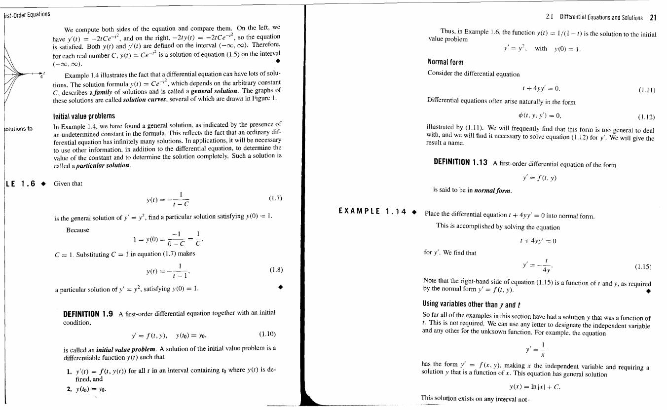
L E 1 . 6 + Given that
I I is the general solution of y' = y2, find a particular solution satisfying y(0) = 1.
Because
1 C = 1. Substituting C = 1 in equation (1.7) makes
a particular solution of y' = y2, satisfying y (0) = 1. +
DEFINITION 1.9 A first-order differential equation together with an initial condition,
is called an initial value problem. A solution of the initial value problem is a differentiable function y ( t ) such that
1. y l ( t ) = f ( t , y ( t ) ) for all t in an interval containing to where y( t ) is de- fined, and
2. y(t0) = yo.
2.1 Differential Equations and Solutions 21
Thus, in Example 1.6, the function y ( t ) = 1/(1 - t ) is the solution to the initial value problem
y' = y2 , with y (0) = 1
Normal form Consider the differential equation
t + 4yy' = 0.
Differential equations often arise naturally in the form
@ ( t , Y . y f ) = 0, (1.12) illustrated by ( I . I I ) . We will frequently find that this form is too general to deal with, and we will find it necessary to solve equation (1 .l?) for y ' We will give the result a name.
DEFINITION 1.1 3 A first-order differential equation of the form
is said to be in normal form.
E X A M P E 1 . 1 4 + Place the differential equation t + 4yy' = 0 into normal form.
This is accomplished by solving the equation
for y'. We find that t
y' = --. 4y
Note that the right-hand side of equation (1.1 5 ) is a function of t and y, as required by the normal form y' = f ( t , y). + Using variables other than y and t So far all of the examples in this section have had a solution y that was a function of t . This is not required. We can use any letter to designate the independent variable and any other for the unknown function. For example. the equation
has the form yf = f ( x , y), making x the independent variable and requiring a solution y that is a function of x . This equation has general solution
- This solution exists on any interval not i -
irst-Order Equations
For another example, in the equation
the independent variable is r and the unknown function is i. which must be a func- tion of r . The general solution of this equation is
I This general solution exists on the interval LO, oo).
Interval of existence The interval of existence of a solution to a differential equation is defined to be the largest interval over which the solution can be defined and remain a solution. It is important to remember that solutions to differential equations are required to be differentiable, and this implies that they are continuous. The solution to the initial value problem in Example 1.6 is revealing.
E 1 . 1 6 6 Find the interval of existence for the solution to the initial value problem
).I = y 2 with y(O)= 1 .
In Example 1.6. we found that the solution is
-1 y(l> = -. t - 1
The graph of y is a hyperbola with two branches, as shown in Figure 2 The func- tion y has an infinite discontinuity at t = 1. Consequently, this function cannot be
I / considered to be a solution to the differential equation y' = y2 over the whole real line.
Note that the left branch of the hyperbola in Figure 2 passes through the point (0, I), as required by the initial condition y ( 0 ) = I . Hence, the left branch of the hyperbola is the solution curve needed. This particular solution curve extends indefinitely to the left, but rises to positive infinity as it approaches the asy~nptote
,aph of t = 1 from the left. Any attempt to extend this solution to the right would have to include t = I , at which point the function y ( t ) is undefined. Consequently. the maximum interval on which this solution curve is defined is the interval (-m, 1). This is the interval of existence.
6
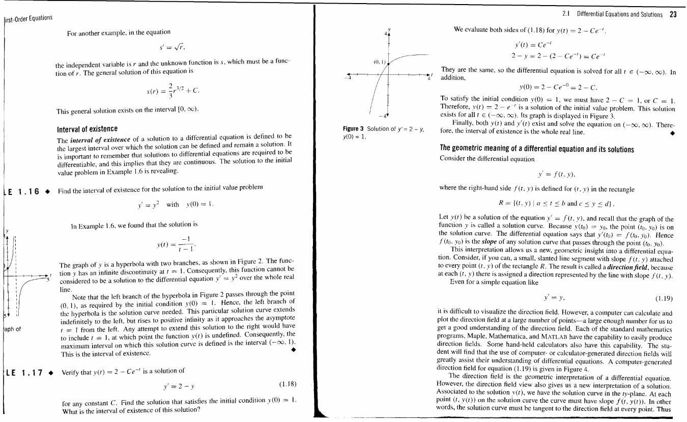
L E 1 . 1 7 6 Verify that y(r) = 2 - Ce-' is a solution of
y 1 = 2 - y
for any constant C . Find the solution that satisfies the initial condition y(0) = 1 . What is the interval of existence of this solution?
2.1 Differential Equations and Solutions 23
4 i
We evaluate both sides of (1.18) for y ( t ) = 2 - Cect .
They are the same, so the differential equation is solved for all t E (-oo, oo). In addition,
0 y ( O ) = 2 - C e - = 2 - C .
To satisfy the initial condition g(0) = 1 , we must have 2 - C = 1, or C = 1. Therefore, v ( r ) = 2 - ec' is a solution of the initial value problem. This solution exists for all t E (-oo, oo). Its graph is displayed in Figure 3.
Finally, both y ( t ) and y f ( t ) exist and solve the equation on (-oo, ca). There- Figure 3 Solution of Y' = 2 - Yl fore, the interval of existence is the whole real line. 6 y(0) = 1.
The geometric meaning of a differential equation and its solutions Consider the differential equation
where the right-hand side f ( t , J ) is defined for ( t , y ) in the rectangle
Let y ( t ) be a solution of the equation y' = f ( t , p), and recall that the graph of the function y is called a solution curve. Because ' ( t o ) = yo, the point (to, yo) is on the solution curve. The differential equation says that yf(ro) = f (to, y o ) Hence J'(to, yo) is the slope of any solution curve that passes through the point (to, yo).
This interpretation allows us a new, geometric insight into a differential equa- tion. Consider, if you can, a small, slanted line segment with slope f ( t . y ) attached to every point (t . p ) of the rectangle R. The result is called a directionjeld, because at each (t, y ) there is assigned a direction represented by the line with slope f ( t , y) .
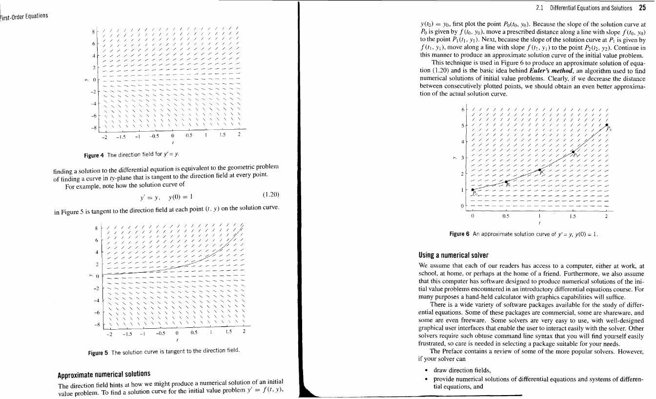
Even for a simple equation like
it is difficult to visualize the direction field. However, a computer can calculate and plot the direction field at a large number of points-a large enough number for us to get a good understanding of the direction field. Each of the standard mathematics programs, Maple, Mathematica. and MATLAB have the capability to easily produce direction fields. Some hand-held calculators also have this capability. The stu- dent will find that the use of computer- or calculator-generated direction fields will greatly assist their understanding of differential equations. A computer-generated direction field for equation (1.19) is given in Figure 4.
The direction field is the geometric interpretation of a differential equation. However, the direction field view also gives us a new interpretation of a solution. Associated to the solution v ( t ) , we have the solution curve in the ry-plane. At each point ( t , y ( t ) ) on the solution curve the curve must have slope f ( t , y ( t ) ) . In other words, the solution curve must be tangent to the direction field at every point. Thus
Iirst-Order Equations
Figure 4 The direction field for y '= y.
finding a solution to the differential equation is equivalent to the geometric problem of finding a curve in 0-plane that is tangent to the direction field at every point.
For example, note how the solution curve of
in Figure 5 is tangent to the direction field at each point ( t , y) on the solution curve.
Figure 5 The solution curve is tangent to the direction field.
Approximate numerical solutions The direction field hints at how we fight produce a numerical solution of an initial value problem. To find a solution curve for the initial value problem y' = f ( t , y ) ,
2.1 Differential Equations and Solutions 25
y(to) = yo, first plot the point Po(to, yo). Because the slope of the solution curve at Po is given by f (to, yo), move a prescribed distance along a line with slope f ( to, yo) to the point PI ( t l , y l ) . Next, because the slope of the solution curve at PI is given by f ( t l , y l ) , move along a line with slope f ( t l , y I ) to the point P2(t2, y2). Continue in this manner to produce an approximate solution curve of the initial value problem.
This technique is used in Figure 6 to produce an approximate solution of equa- tion (1.20) and is the basic idea behind Euler's method, an algorithm used to find numerical solutions of initial value problems. Clearly, if we decrease the distance between consecutively plotted points, we should obtain an even better approxima- tion of the actual solution curve.
Figure 6 An approximate solution curve of y ' = y, y(0) = 1.
Using a numerical solver We assume that each of our readers has access to a computer, either at work, at school, at home, or perhaps at the home of a friend. Furthermore, we also assume that this computer has software designed to produce numerical solutions of the ini- tial value problems encountered in an introductory differential equations course. For many purposes a hand-held calculator with graphics capabilities will suffice.
There is a wide variety of software packages available for the study of differ- ential equations. Some of these packages are commercial, some are shareware, and some are even freeware. Some solvers are very easy to use, with well-designed graphical user interfaces that enable the user to interact easily with the solver. Other solvers require such obtuse command line syntax that you will find yourself easily frustrated, so care is needed in selecting a package suitable for your needs.
The Preface contains a review of some of the more popular solvers. However, if your solver can
draw direction fields, provide numerical solutions of differential equations and systems of differen- tial equations, and
t,t-l)rder Equations
plot solutions of differential equations and systems of differential equations,
then your solver will be adequate for use with this text.
Test drive your solver Let's test our solvers in order to assure ourselves that they will provide adequate support for the material in this text.
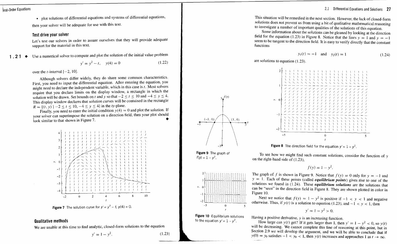
1 . 2 1 + Use a numerical solver to compute and plot the solution of the initial value problem
over the t-interval [-2, 101.
Although solvers differ widely, they do share some common characteristics. First, you need to input the differential equation. After entering the equation, you might need to declare the independent variable, which in this case is t . Most solvers require that you declare limits on the display window, a rectangle in which the solution will be drawn. Set bounds on t and y so that -2 _( t 5 10 and -4 5 y 5 4. This display window declares that solution curves will be contained in the rectangle R = {(t, y) 1 -2 5 t 5 10, -4 5 y 5 4) in the ty-plane.
Finally, you need to enter the initial condition y (4) = 0 and plot the solution. If your solver can superimpose the solution on a direction field, then your plot should look similar to that shown in Figure 7. +
Figure 7 The solution curve for y '= y2 - t, y(4) = 0.
Qualitative methods We are unable at this time to find analytic, closed-form solutions to the equation
Figure 9 The graph of f(y) = 1 - y2.
Figure 10 Equilibrium solutions to the equation y l = 1 - y2.
2.1 Differential Equations and Solutions 27
This situation will be remedied in the next section. However, the lack of closed-form solutions does not prevent us from using a bit of qualitative mathematical reasoning to investigate a number of important qualities of the solutions of this equation.
Some information about the solutions can be gleaned by looking at the direction field for the equation (1.23) in Figure 8. Notice that the lines y = 1 and y = -1 seem to be tangent to the direction field. It is easy to verify directly that the constant functions
y ~ ( t ) = - l and y 2 ( t ) = 1 (1.24)
are solutions to equation (1.23).
Figure 8 The direction field for the equation y '= 1 - y2.
To see how we might find such constant solutions, consider the function of y on the right-hand side of (1.23),
The graph of f is shown in Figure 9. Notice that f (y) = 0 only for y = -1 and y = I . Each of these points (called equilibrium poirlts) gives rise to one of the solutions we found in (1.24). These equilibrium solutions are the solutions that can be "seen" in the direction field in ~ i ~ u r e 8. They are shown plotted in color in Figure 10.
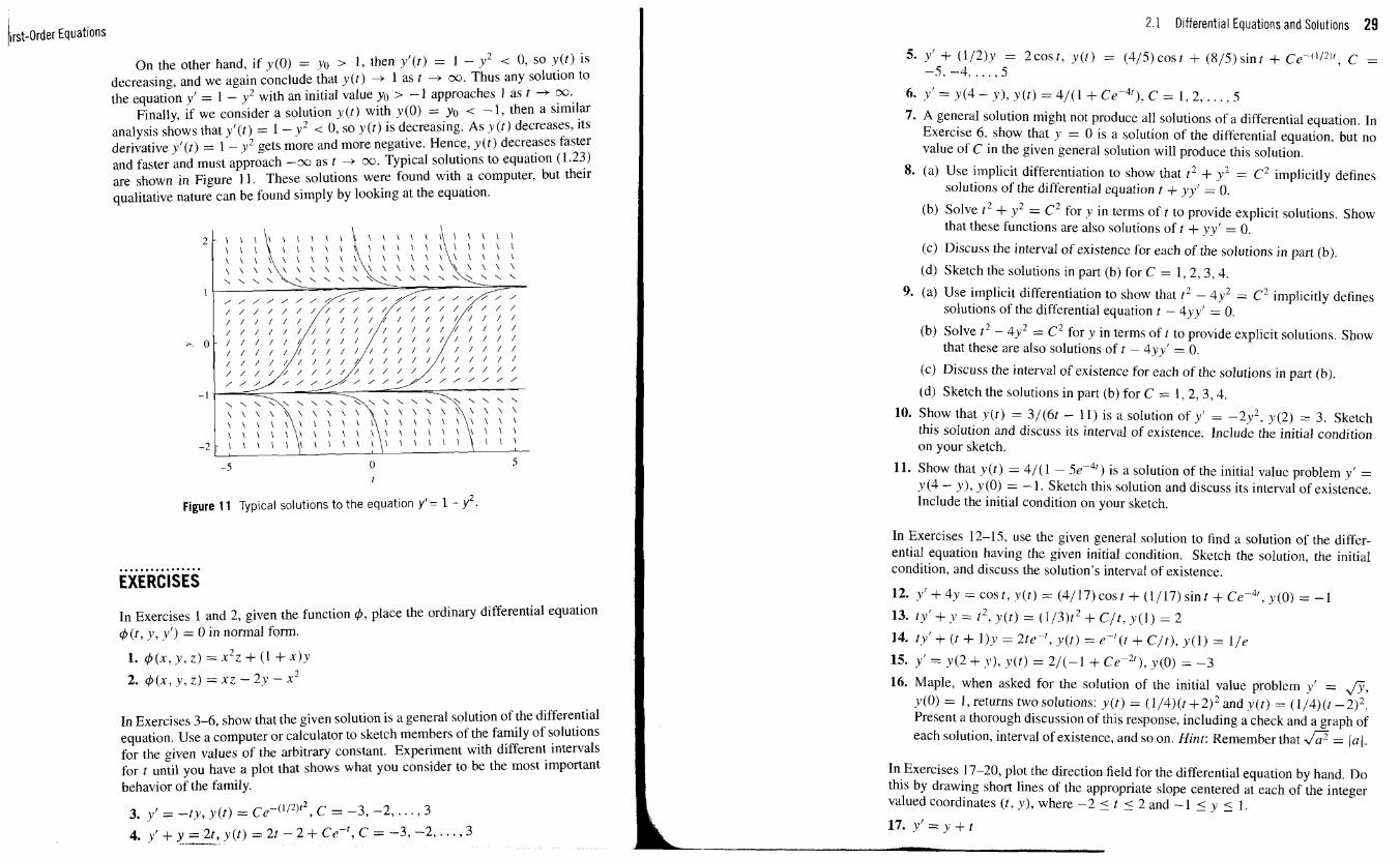
Next we notice that f (y) = I - y2 is positive if -1 < y < 1 and negative otherwise. Thus, if y(t) is a solution to equation (1.23), and -1 < y < 1, then
Having a positive derivative, y is an increasing function. How large can y (t) get? If it gets larger than 1, then y' = 1 - y2 < 0, so y (t)
will be decreasing. We cannot complete this line of reasoning at this point, but in Section 2.9 we will develop the argument, and we will be able to conclude that if y (0) = yo satisfies - 1 < yo < 1, then y (t) increases and approaches 1 as t + oo. -
/rst-order Equations
On the other hand, if y(0) = yo > 1, then yl(t) = 1 - y2 < 0, so y(t) is decreasing, and we again conclude that y (t) + 1 as t i oo. Thus any solution to the equation y' = 1 - y2 with an initial value yo > -1 approaches 1 as t -+ oo.
Finally, if we consider a solution y (r) with y(0) = yo - 1, then a similar
analysis shows that yl(t) = 1 - y2 < 0, so y(t) is decreasing. As y(r) decreases, its derivative yl(t) = 1 - y2 gets more and more negative. Hence, y ( r ) decreases faster and faster and must approach -oo as t + cm. Typical solutions to equation (1.23) are shown in Figure 11. These solutions were found with a computer, but their qualitative nature can be found simply by looking at the equation.
Figure 11 Typical solutions to the equation y l = 1 - y2.
................ EXERCISES
In Exercises 1 and 2, given the function 4, place the ordinary differential equation 4 (r, y, y') = 0 in normal form.
In Exercises 3-6, show that the given solution is a general solution of the differential equation. Use a computer or calculator to sketch members of the family of solutions for the given values of the arbitrary constant. Experiment with different intervals for t until you have a plot that shows what you consider to be the most important behavior of the family.
3. y' = -ty, y(t) = ~ e - ( l l ' ) ' ~ , C = -3, -2.. . . . 3
4. y' + y = 2t, y (t) = 2t - 2 + Ce-', C = -3, -2, . . . , 3 --
2.1 Differential Equations and Solutions 29
5. y' + (1/2)y = 2 cos t, y ( t ) = (415) cos t + (815) sin t + ~ e - ( ' / ~ ) ' , C = -5, -4, . . . . 5
7. A general solution might not produce all solutions of a differential equation. In Exercise 6, show that y = 0 is a solution of the differential equation, but no value of C in the given general solution will produce this solution.
8. (a) Use implicit differentiation to show that t2 + y2 = c2 implicitly defines solutions of the differential equation t + yyt = 0.
(b) Solve t2 + y2 = c2 for y in terms of t to provide explicit solutions. Show that these functions are also solutions o f t + yy' = 0.
(c) Discuss the interval of existence for each of the solutions in part (b).
(d) Sketch the solutions in part (b) for C = 1, 2 ,3 ,4 .
9. (a) Use implicit differentiation to show that t2 - 4y2 = C2 implicitly defines solutions of the differential equation t - 4yy' = 0.
(b) Solve t 2 - 4y2 = c2 for y in terms of t to provide explicit solutions. Show that these are also solutions o f t - 4yy' = 0.
(c) Discuss the interval of existence for each of the solutions in part (b).
(d) Sketch the solutions in part (b) for C = 1,2, 3 ,4 .
10. Show that y ( t ) = 3/(6t - 11) is a solution of y' = -2y2, y(2) = 3. Sketch this solution and discuss its interval of existence. Include the initial condition on your sketch.
11. Show that y(t) = 4/(1 - 5ec4') is a solution of the initial value problem y' = y (4 - y), y (0) = -1. Sketch this solution and discuss its interval of existence. Include the initial condition on your sketch.
In Exercises 12-15, use the given general solution to find a solution of the differ- ential equation having the given initial condition. Sketch the solution, the initial condition, and discuss the solution's interval of existence.
13. ty' + .v = t2, y(t) = (1/3)t2 + C l t , y(1) = 2
14. ty' + (r + l )y = 2teP', y(t) = r-'(t + C/t), y(1) = l / e
16. Maple, when asked for the solution of the initial value problem y' = a, y(0) = 1, returns two solutions: y(t) = (1/4)(t+212 and y(t) = (1/4)(t -2)2. Present a thorough discussion of this response, including a check and a graph of each solution, interval of existence, and so on. Hint: Remember that @ = (a ( .
In Exercises 17-20, plot the direction field for the differential equation by hand. Do this by drawing short lines of the appropriate slope centered at each of the integer valued coordinates ( t , y), where -2 5 t 5 2 and - 1 5 y 5 1.
17. y ' = y + t
I rst-Order Equations
In Exercises 21-24, use a computer to draw a direction field for the given first-order differential equation. Use the indicated bounds for your display window. Obtain a printout and use a pencil to drdw a number of possible solution trajectories on the direction field. If possible, check your solutions with a computer.
- 3 < t ( 3 , - 5 5 y ' S ) 21. y' = -ty, R = {(t, V ) . -
22. y' = y2 - t , R = { ( t , y) : -2 I t I 10, -4 5 y 5 4)
23. y ' = t - y + I, R = {(t, y ) : -6 I t 1 6 , -6 I Y 5 6 )
24. y' = (y + t)/(y - t), R = {(t, y) : -5 5 t 5 5, -5 I Y 5 51
For each of the initial value problems in Exercises 25-28, use a numerical solver to plot the solution curve over the indicated interval. Try different display windows by experimenting with the bounds on y. Note: Your solver might require that you first place the differential equation in normal form.
26. y' + ty = t2, y(0) = 3, t E [-4,41
27. y' - 3y = sint, y(0) = -3, t E [-6~r, n/41
28. v' + (cos t)y = sin t , y (0) = 0, r E [-lo. 101
Some solvers allow the user to choose dependent and independent variables. For example, your solver may allow the equation r' = -2sr + e-', but other solvers will insist that you change variables so that the equation reads y' = -2ty + e-'. or y' = -2xy + e-', should your solver require x as the independent variable. For each of the initial value problems in Exercises 29 and 30, use your solver to plot solution curves over the indicated interval.
In Exercises 31-34, plot solution curves for each of the initial conditions on one set of axes. Experiment with the different display windows until you find one that exhibits all of the important behavior of your solutions. Note: Selecting a good display window is an art, a skill developed with experience. Don't become overly frustrated in these first attempts.
31. y' = y(3 - y), y(0) = -2, -1,O, 1 ,2 , 3 , 4 , 5
32. x ' - x 2 =t ,x(O) = -2,0,2,x(2) =O,x(4) = -3 ,0 ,3 ,x(6) = O
2.2 Solutions to Separable Equations 31
In Exercises 35-38. the exact solution accompanies each initial value problem. (i) Verify that the y (t) is a solution of the initial value problem.
(ii) Use your numerical solver to plot the solution of the initial value uroblem. (iii) Plot thz graph of y(t) and compare with the numerical solution found in part
(ii).
37. y' + 4y = cost + sint. y(0) = 1, y(t) = (3/17)cost + (5/17)sint + (14/17)e-~'
38. y' = ty, y(O) = 2, y(1) = 2e('/2"2
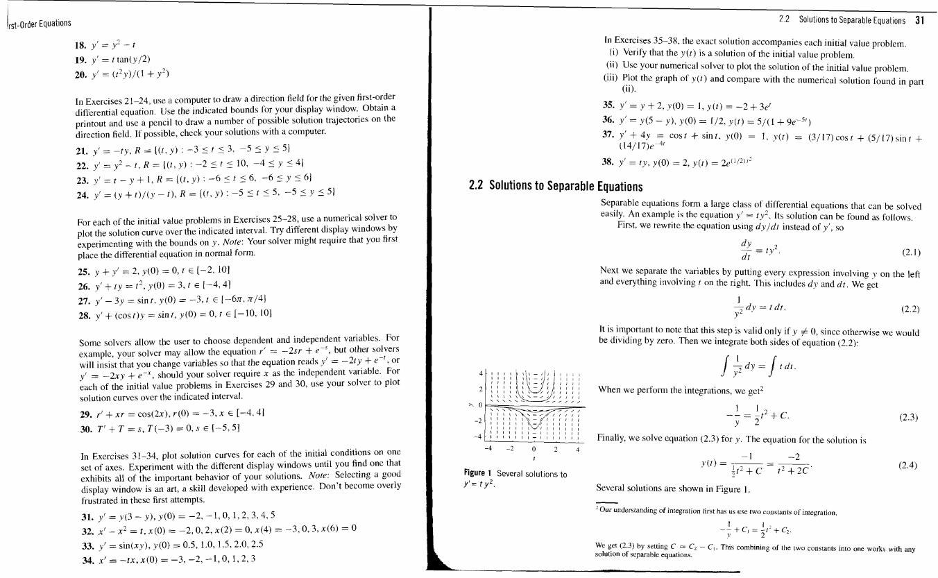
2.2 Solutions to Separable Equations Separable equations form a large class of differential equations that can be solved easily. An example is the equation y' = ty2. Its solution can be found as follows.
First, we rewrite the equation using dy/dt instead of y', so
Next we separate the variables by putting every expression involving y on the left and everything involving t on the right. This includes d y and dt . We get
I -dy = t d t . y2 (2.2)
It is important to note that this step is valid only if y # 0, since otherwise we would be dividing by zero. Then we integrate both sides of equation (2.2):
C l . f dt .
1 1 1 1 1 ) - I ! 1 1 1 1
2 I I I I ~ l \ \ : / t I I I I I When we perform the integrations. we get2 \ \ \ \ \ \ \ - / , , , / I , \\\..- //.,,, 1 I
I l l \ \ \-,- / / / I t -- - - St2 + c. I I l \ i \ \ - / I I I I I I -2 l l l l l ! \ - ~ ! ! l l 1 1
I I I I I I \ I I I I I I I l l I I I l 1 - l J I I O I
-4 1 I I I - I I I I I Finally, we solve equation (2.3) for v . The equation for the solution is
Figure 1 Several solutions to Y ' = t y 2 . Several solutions are shown in Figure I
- 'Our understanding of integration first has us use two constants of integration,
We get (2.3) by setting C = CZ - CI. This combining of the two constants into one works with any
L solution of separable equations.
Irst-0rder Equations
Treating dy and d t as mathematical entities, as we did in separating the vari- ables in equation (2.2), may be troublesome to you. If so, it is probably because you have learned your calculus very well. We will explain this step at the end of this section under the heading "Why separation of variables works."
The general method Clearly the key step in this method is the separation of variables. This is the step going from equation (2.1) to equation (2.2). The method of solution illustrated here will work whenever we can perform this step, and this can be done for any equation of the two equivalent forms
and
Equations of either form are called separable differential equations. For both we can separate the variables; for example, for equation (2.6), we get
(We must be careful here to avoid those points where f ( y ) = 0.) We can integrate both sides of this equation,
Thus we can find the solution to separable equations by perfornling two integrations. An equation in the form of (2.5) can be handled in a similar manner.
What about those points where f ( y ) = 0 in equation (2.6)? It turns out to be quite easy to find the solutions in such a case, since if f (yo) = 0 , then by substitution we see that the constant function y ( t ) = 4'0 is a solution 2 to (2.6). In particular, the function y ( t ) = 0 is a solution to the equation 3,' = tv .
Let's look at some examples.
I L E 2 . 7 + Consider the equation x' = r x , where r is an arbitrary constant and r is the assumed independent variable.
This equation is perhaps the one that arises most in applications. We will see it often. Because of the form of its solutions, it is called the exponential equation. The equation is separable, so we rewrite it as
dx - = r x , dr
(2.8)
2.2 Solutions to Separable Equations 33
and then we separate the variables to obtain
1 - dx = r dt. X (2.9)
In doing so we have to be cautious about dividing by zero, so for now we insist that x #O.
We want to integrate (2.9), but there is a slight hitch with the left-hand side of the equation. If x > 0, then / ( l / x ) d x = In x, but what if x < O? In this case, we have j ( l / x ? dx = In(-x). Hence, when we integrate both sides of equation (2.9), it becomes
It remains to solve for x . Taking the exponential of both sides of equation (2.10), we get
I x ( t ) 1 = er'+c = ecer'.
Since eC and err are both positive, there are two cases
We can simplify the solution by introducing
eC, i f x > 0 ; -eC, i fx ( 0 .
Therefore, the solution is also described by the simpler formula
where A is a constant different from zero, but otherwise arbitrary. In arriving at equation (2.9), we divided both sides of equation (2.8) by x, and
this procedure is not valid when x = 0. However, as we pointed out before this example, t h s means that n = 0 is a solution of the original equation, x' = r x . Consequently, the solution
~ ( t ) = Aer', (2.12)
where A is completely arbitrary, gives us the solution in all cases. + E X A M P L E 2 . 1 3 + Find a solution to the initial value problem y' = 0.3y with j(0) = 4.
This is a special case of the equation in Example 2.7. Therefore, we know that the general solution is
y ( t ) = ~ e ' . ~ ' .
Substituting t = 0 and using the initial condition, we get
4 = y (0 ) = A .
Hence A = 4 and our solution is y ( t ) = 4e0.3'. +
! rst-Order Equations
Using definite integration Sometimes it is useful to use definite integrals when solving initial value problems for separable equations.
E 2 . 1 4 + Solve the differential equation y' = ry with y(0) = 3.
The equation is separable, so we first rewrite it as
dy - = ty. dt
Separating variables, we get dy - = t d t . Y
The next step is to integrate both sides, but this time let's use definite integrals to bring in the initial condition y (0) = 3. Thus t = 0 corresponds to y = 3, and we have
Notice that we changed the variables of integration because we want the upper limits of our integrals to be y and t. Performing the integration, we get
We can solve for y by exponentiating, and our answer is
Let's look back at equation (2.15). where we implemented the initial condition. In general, the initial condition is of the form y(to) = yo. Thust = to corresponds to y = yo. These are the initial points for our integrals, and equation (2.1 5) becomes
This integrates to - -
When we solve for y, we get
2.2 Solutions t o Separable Equations 35
Implicitly defined solutions After the integration step, we need to solve for the solution. However, this is not always easy. In fact, it is not always possible. We will look at a series of examples.
E X A M P E 2 . 1 6 + Consider the equation r' = (cos u)/r: where u is the independent variable. We will be interested in the initial conditions r(0) = 1 and r (0) = - 1 .
We rewrite the equation and separate the variables,
d r cosu - or r d r = c o s u d u . clu r
Integrating, we get
1 -r2 = sin 1~ + C or r 2 = 2 sin i r + 2C. 2
To simplify things slightly, replace the constant 2C by D, so
2 r = 2sinu + D. (2.17) r
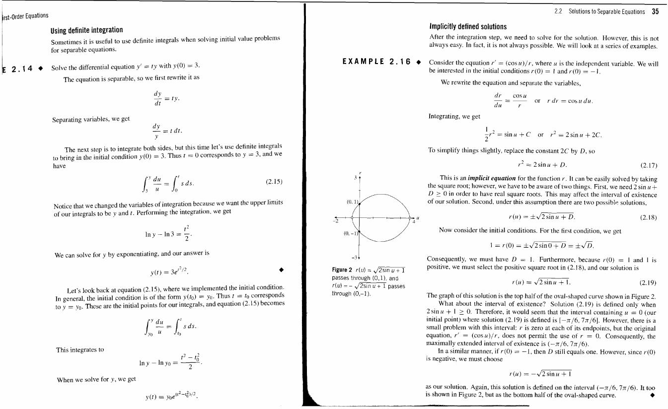
This is an implicit equation for the function r . It can be easily solved by taking the square root; however, we have to be aware of two things. First, we need 2 sin u + D > 0 in order to have real square roots. This may affect the interval of existence of our solution. Second. under this assumption there are two possible solutions,
. : r(u) = k2/2 sin u + D. -2 (2.18)
Now consider the initial conditions. For the first condition, we get
I = r(O) = k J2sin0 + D = k f i .
-3 4 Consequently, we must have D = I . Furthermore, because r(0) = I and 1 is Figure 2 r (u) = 2 / Z E E i positive. we must select the positive square root in (2.18), and our solution is
passes through (0,1), and r ( u ) = - 2/- passes through (0,-1). The graph of this solution is the top half of the oval-shaped curve shown in Figure 2.
What about the interval of existence? Solution (2.19) is defined only when 2 sin u + 1 2 0. Therefore, it would seem that the interval containing u = 0 (our initial point) where solution (2.19) is defined is [-n/6,7n/6]. However, there is a small problem with this interval: r is zero at each of its endpoints, but the original equation, r ' = (cosu)/r, does not permit the use of r = 0. Consequently, the maximally extended interval of existence is (-n/6. 7x16).
In a similar manner, if r (0) = -1, then D still equals one. However, since r (0) is negative, we must choose
as our solution. Again, this solution is defined on the interval (-n/6, 7n/6). It too is shown in Figure 2, but as the bottom half of the oval-shaped curve. +
p - o r d e r Equations
Let's be sure we know what the terminology means. An explicit solution is one for which we have a formula that is a mathematical expression involving only the independent variable. Such a formula enables us, in theory at least, to calculate it. For example, (2.19) is an explicit solution to the equation in the previous example. In contrast, (2.17) is an implicit equation for the solution. In this example, the implicit equation can be solved easily, but this is not always the case.
Unfortunately, implicit solutions occur frequently. Consider again the general problem in the form dyldr = g(r)/ h(y). Separating variables and integrating. we get
If we let
H(y) = \ My) dy and GO) = \ g(t) dl. l
and then introduce a constant of integration, equation (2.20) can be rewritten as
H(y) = G(t) + C. (2.21)
Unless H(y) = y, this is an implicit equation for y(t). To find an explicit solution we must be able to compute the inverse function H - ' . If this is possible, then we have
Let's look at a slightly more complicated example.
. E 2 . 2 2 + Find the solutions of the equation y' = e" / (1 + y), having initial conditions y (0) = 1 and y(0) = -4.
Separate the variables and integrate.
1 2 ~ + ~ y = e X + C
t Rearrange equation (2.23) as
y2 + 2y - 2(e-' + C) = 0.
If \ This is an implicit equation for y (x) that we can solve using the quadratic formula.
(0, 11, while - = -1 f J1 +2(ex + C) ?ex passes
Again we get two solutions from the quadratic formula, and the initial condition will dictate which solution we choose. If y(0) = 1, then we must use the positive square root and we find that C = 112. The solution is
y(x) = -1 +&?G. (2.24) > -- .- ..- . -
2.2 Solutions to Separable Equations 37
On the other hand, if y(0) = -4, then we must use the negative square root and we find that C = 3. The solution in this case is
Both solutions are shown in Figure 3. What about the interval of existence? A quick glance reveals that each solution
is defined on the interval (-ca, oo). Some calculation will reveal that y'(x) is also defined on (-ca. ca). However, for each solution to satisfy the equation y' = eX/(l + y), y must not equal -1. Fortunately, neither solution (2.24) or (2.25) can ever equal - 1. Therefore, the interval of existence is (-ca, ca). +
Let's do one more example.
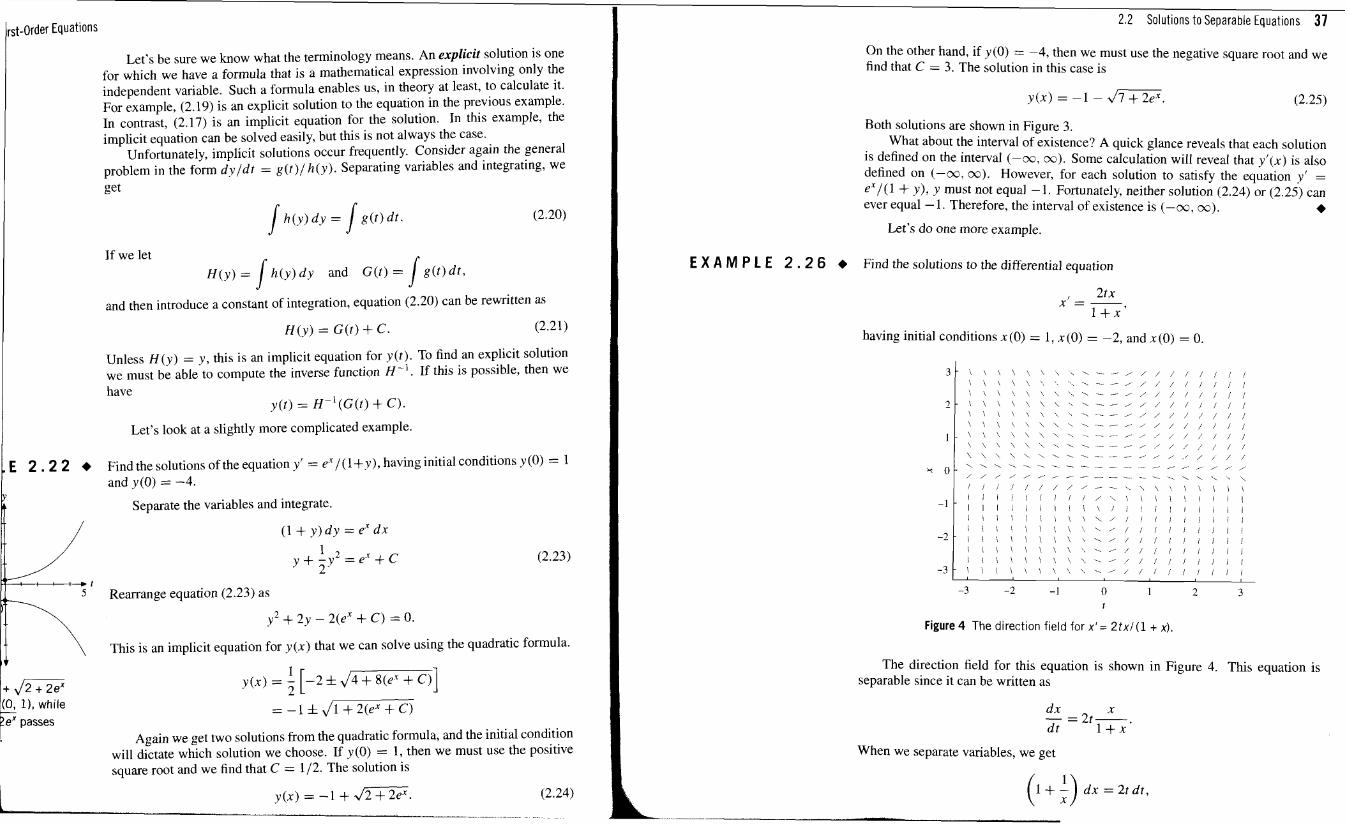
E X A M P E 2 . 2 6 + Find the solutions to the differential equation
having initial conditions x (0) = 1, x (0) = -2, and x (0) = 0.
Figure 4 The direction field for x ' = 2 t x l ( 1 + x).
The direction field for this equation is shown in Figure 4. This equation is separable since it can be written as
When we separate variables, we get
(1 + -!) dx = 2f df, L--
irst-Order Equations I assuming that x # 0 . Integrating, we get
where C is an arbitrary constant. For the initial condition x ( 0 ) = I , this becomes I = C. Hence our solution is implicitly defined by
This is as far as we can go. We cannot solve equation (2.28) explicitly for x ( t ) , so we have to be satisfied with this as our answer. The solution x is defined implicitly by equation (2.28).
For the initial condition x ( 0 ) = -2, we can find the constant C in the same manner. We get -2 + In(\ - 21) = C , or C = In 2 - 2. Hence the solution is defined implicitly by
2 .r + ln(l.xJ) = t + In2 - 2 .
Our initial condition is negative, so our solution must also be negative. Hence 1x1 = -.r, and our final implicit equation for the solution is
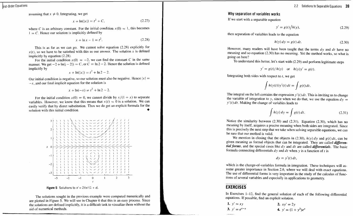
For the initial condition x ( 0 ) = 0 , we cannot divide by x / ( l + x) to separate variables. However, we know that this means that .r(t) = 0 is a solution. We can easily verify that by direct substitution. Thus we do get an explicit formula for the solution with this initial condition.
Figure 5 Solutions to x ' = 2 t x / ( l + x).
The solutions sought in the previous example were computed numerically and are plotted in Figure 5. We will see in Chapter 6 that this is an easy process. Since the solutions are defined implicitly, it is a difficult task to visualize them without the aid of numerical methods.
2.2 Solutions to Separable Equations 39
Why separation of variables works If we start with a separable equation
then separation of variables leads to the equation
However, many readers will have been taught that the terms d y and d t have no meaning and so equation (2.30) has no meaning. Yet the method works, so what is going on here?
To understand this better, let's start with (2.29) and perform legitimate steps
Integrating both sides with respect to t , we get
The integral on the left contains the expression y l ( t ) d t . This is inviting us to change the variable of integration to y , since when we do that, we use the equation d y = y ' ( t ) d t . Making the change of variables leads to
Notice the similarity between (2.30) and (2.31). Equation (2.30), which has no meaning by itself, acquires a precise meaning when both sides are integrated. Since this is precisely the next step that we take when solving separable equations, we can be sure that our method is valid.
We mention in closing that the objects in (2.30), h ( y ) d y and g ( t ) d t , can be given meaning as formal objects that can be integrated. They are called difSeren- tial forms, and the special cases like dy and d t are called differentials. The basic formula connecting differentials d y and d t when y is a function of t is
d y = ~ ' ( t ) d t ,
which is the change-of-variables formula in integration. These techniques will as- sume greater importance in Section 2.6, where we will deal with exact equations. The use of differential forms is very important in the study of the calculus of func- tions of several variables and especially in applications to geometry.
................ EXERCISES In Exercises 1-12, find the general solution of each of the following differential equations. If possible, find an explicit solution.
2. xy' = 2y
4. y' = ( 1 + y2)eX
irst-order Equations
5. y' = xy + y 6. y' = ye' - 2e' + y - 2
7. y' = x/(y + 2) 8. y ' = xyl(x - 1) 1 r 9. s-y = y In y - y' 10. xy' - y = 2x2y
11. y3y' = x + 2y' 12. "' = (2xy + 2x)/(x2 - I)
In Exercises 13-18, find the exact solution of the initial value problem. Indicate the interval of existence.
In Exercises 19-22, find exact solutions for each given initial condition. State the interval of existence in each case. Plot each exact solution on the interval of exis- tence. Use a numerical solver to duplicate the solution curve for each initial value problem.
An unstable nucleus is radioactive. At any instant, it can emit a particle, trans- forming itself into a different nucleus in the process. For example, 2 3 x ~ is an alpha emitter that decays spontaneously according to the scheme 2 3 8 ~ 4 2 3 4 ~ h + ' ~ e , where 'He is the alpha particle. In a sample of 2 3 x ~ , a certain percentage of the nuclei will decay during a given observation period. If at time t the sample contains N (t) radioactive nuclei, then we expect that the number of nuclei that decay in the time interval At will be approximately proportional to both N and At. In symbols,
AN = N(t + At) - N(t) -hN(t)dt, (2.32)
where h is a constant of proportionality. Use this fact to solve Exercises 23-26.
23. Show that N (t) satisfies the differential equation
24. If No represents the number of 2 " ~ nuclei present at time t = 0, use equa- tion (2.33) to show that the number of 2 3 8 ~ present at time t is given by the equation
N (r ) = ~oe-" . (2.34)
2.2 Solutions to Separable Equations 41
25. The half--life of a radioactive substance is defined as the amount of time that it takes one-half of the substance to decay. Show that the half-life of the defined by equation (2.34), is given by the formula
26. The half-life of 2 3 8 ~ is 4.47 x lo7 yr.
(a) Use equation (2.35) to compute the decay constant h for 2 3 8 ~ .
(b) Suppose that 1000 mg of '"u are present initially. Use equation (2.34) and the decay constant determined in part (a) to determine the time for this sample to decay to 100 mg.
27. "P, an isotope of phosphorus, is used in leukemia therapy. After 10 hours, 615 mg of a 1000-mg sample remain. Determine the half-life of 3 2 ~ .
28. Tritium, 9, is an isotope of hydrogen that is sometimes used as a biochemical tracer. Suppose that 100 mg of % decays to 80 mg in 4 hours. Determine the half-life of 3 ~ .
29. The isotope Technitium 99m is used in medical imaging. It has a half-life of about 6 hours, a useful feature for radioisotopes that are injected into humans. The Technitium, having such a short half-life, is created artificially on scene by harvesting it from a more stable Molybdenum isotope, 9 9 ~ b . If 10 g of 9 9 ' n ~ c are "harvested" from the Molybdenum, how much of this sample remains after 9 hours?
30. The isotope Iodine 13 1 is used to destroy tissue in an overactive thyroid gland. It has a half-life of 8.04 days. If a hospital receives a shipment of 500 mg of I" I, how much of the isotope will be left after 20 days?
In the laboratory, a more useful measurement is the decay rate R, usually measured in disintegrations per second, counts per minute, etc. Thus, the decay rate is de- fined as R = -dN/dt. Using equation (2.33), it is easily seen that R = AN. Furthermore, differentiating (2.34) with respect to t reveals that
in which Ro is the decay rate at t = 0. That is, because R and N are proportional, they both decrease with time according to the same exponential law.
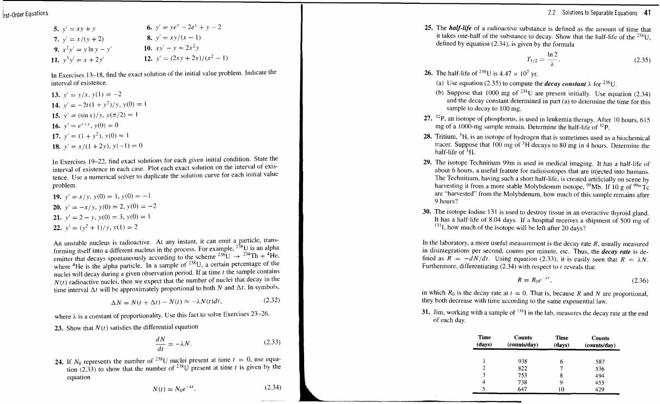
31. Jim, working with a sample of I3'l in the lab, measures the decay rate at the end of each day.
Time Counts Time Counts (days) (countslday) (days) (countdday)
Ir~t-Order Equations 2.2 Solutions to Separable Equations 43
Taking the natural logarithm of both sides of equation (2.36) produces the result
Therefore, plotting In R versus t should produce a line with slope -h. On a sheet of graph paper, plot the natural logarithm of the decay rates versus the time, and then estimate the slope of the line of best fit. Use this estimate to approximate the half-life of 13'1.
32. A 1.0-g sample of Radium 226 is measured to have a decay rate of 3.7 x 10'O disintegrationsls. What is the half-life of ' "~a in years? Note: A chemical constant, called Avogadro's number, says that there are 6.02 x 10" atoms per mole, a common unit of measurement in chemistry. Furthermore, the atomic mass of 2 2 h ~ a is 226 glmol.
33. A substance contains two Radon isotopes, 2 ' 0 ~ n [ t ~ , ~ = 2.42 h] and 2 1 1 ~ n [t1/2 = 15 h ] At first, 20% of the decays come from "'Rn How long must one wait until 80% do so?
34. Radiocarbon dating. Carbon 14 is produced naturally in the earth's atmo- sphere through the interaction of cosmic rays and Nitrogen 14. A neutron comes along and strikes a nucleus, knoclung off a proton and creating a I4c atom. This atom now has an affinity for oxygen and quickly oxidizes as a 14c02 molecule, which has many of the same chemical properties as regu- lar C02. Through photosynthesis. the 14c02 molecules work their way into the plant system, and from there into the food chain. The ratio of to regular car- bon in living things is the same as the ratio of these carbon atoms in the earth's atmosphere, which is fairly constant, being in a state of equilibrium. When a living being dies, it no longer ingests "C and the existing "C in the now de- funct life form begins to decay. In 1949, Willard F. Libby and his associates at the University of Chicago measured the half-life of this decay at 5568 f 30 years, which to this day is known as the Libby half-life. We now know that the half-life is closer to 5730 years, called the Cambridge half-life, but radiocar- bon dating labs still use the Libby half-life for technical and historical reasons. Libby was awarded the Nobel p r i ~ e in chemistry for his discovery.
(a) Carbon 14 dating is a useful dating tool for organisms that lived during a specific time period. Why is that? Estimate this period.
(b) Suppose that the ratio of to carbon in the charcoal on a cave wall is 0.617 times a similar ratio in living wood in the area. Use the Libby half- life to estimate the age of the charcoal.
35. Newton's law of cooling asserts that the rate at which an object cools is propor- tional to the difference between the object's temperature (T) and the tempera- ture of the surrounding medium (A) . (a) Show that
T = A + (To - A)ePk',
where To is the temperature of the body at time t = 0 and k is the propor- tionality constant.
(b) A murder victim is discovered at midnight and the temperature of the body is recorded at 3 1°C. One hour later, the temperature of the body is 29°C.
Assume that the surrounding air temperature remains constant at 21°C. Calculate the victims' time of death. Note: The "normal" temperature of a living human being is approximately 37°C.
36. Suppose a cold beer at 40°F is placed into a warm room at 70°F. Suppose 10 minutes later, the temperature of the beer is 48°F. Use Newton's law of cooling to find the temperature 25 minutes after the beer was placed into the room.
37. Referring to the previous problem, suppose a bottle of beer at 50°F is discov- ered on a kitchen counter in a 70°F room. Ten minutes later, the bottle is 60°F. If the refrigerator is kept at 40°F, how long had the bottle of beer been sitting on the counter when it was first discovered?
38. Consider the equation
y' = f ( a t + by +c ) , where a , 0, and c are constants. Show that the substitution x = a t + by + c changes the equation to the separable equation .wf = a +bf(x). Use this method to find the general solution of the equation y' = (y + t)2.
39. Suppose a curve y = f (x) lies in the first quadrant and suppose that for each x, the piece of the tangent line at (x, y(x)) which lies in the first quadrant is bisected by the point (x, y(.r)). Find y(x).
40. Suppose the projection of the part of the line normal to the graph of y = y (x) from the point (x. y(x)) to the x-axis has length 2. Find y(.r).
41. Suppose a polar graph r = r(8) has the property that 6 always equals twice the angle from the radial line (i.e., the line from the origin to (8, r(8))) to the tangent. Find the function r(8).
42. Suppose y(x) is a continuous, nonnegative function with y(0) = 0. Find y(x) if the area under the curve y = y(t) from 0 to x is always equal to one-fourth the area of the rectangle with vertices at (0.0) and (x, y(x)).
43. A football, in the shape of an ellipsoid, is lying on the ground in the rain. Its length is 8 inches and its cross section at its widest point is a circular disc of radius 2 inches. A rain drop hits the top half of the football. Find the path that it follows as it runs down the top half of the football. Hint: Recall that the gradient of a function f (x, y) points in the (x, y)-direction of maximum increase of f .
44. From Torricelli's law. water in an open tank will flow through a hole in the bottom at a speed equal to that it would acquire in a free-fall from the level of the water to the hole. A parabolic bowl has the shape of v = x2, 0 5 x 5 1, (units are feet) revolved around the y-axis. This bowl is initially full of water and at t = 0. a hole of radius a is punched at the bottom. How long will it take for the bowl to drain? Hint: An object dropped from height h will hit the ground at a speed of v = J@i where g is the gravitational constant. This formula is derived from equating the kinetic energy of impact, (1/2)mv2, with the work required to raise the object, mgh.
45. Refening to the previous problem, for what function f would the bowl defined by y = f (x) have the property that the water 1- 1
tilSt-0rder Equations
46. A destroyer is hunting a submarine in a dense fog. The fog lifts for a moment, disclosing that the submarine lies on the surface 4 miles away. The subma- rine immediately descends and departs in a straight line in an unknown direc- tion. The speed of the destroyer is three times that of the submarine. What path should the destroyer follow to be certain of intercepting the submarine? Hint: Establish a polar coordinate system with the origin located at the point where the submarine was sighted. Look up the formula for arclength in polar coordinates.
if Motion One of the most intensively studied scientific problems is the study of motion. This is true in particular for the motion of the planets. The history of the ideas involved is one of the most interesting chapters of human history. We will start by giving a brief summary of the development of models of motion.
A hrief history of models of motion
The study of astronomy goes back 3000 years to the Babylonians. Their interest in the stars was furthered by the Greeks, who came up with a descriptive model of the motion of the planets. They assumed that the earth was the center of the universe and that everything revolved around the earth. At first they thought that the planets moved in circular paths around the earth, but as they grew more proficient in their measurements they realized that this was not true. They modified their theory by inventing epicycles. These were smaller circles, the centers of which moved along circular arcs centered at the earth. The planets moved along the epicycles as the epicycles moved around the earth. When this theory proved to be inadequate in some cases, the Greeks added epicycles to the epicycles.
The theory of epicycles enabled the Greeks to compute and predict the motion of the planets. In many ways it was a highly satisfactory scientific theory. However, it left many questions unanswered. Most important, why do the planets have such a complicated motion as that suggested by the theory of epicycles? There was no causal explanation of why the use of epicycles predicted the motion of the planets. Their theory was only descriptive in nature.
A major improvement on this theory came in 1543. when Copernicus made the radical suggestion that the earth was not the center of the universe. Instead, he proposed that the sun was the center. Of course this required a major change in the thinking of all humankind in matters of religion and philosophy as well as in astronomv. It did, however, make the theory of epicycles somewhat easier, because .
fewer epicycles were needed to explain the motion of the planets. Starting in 1609, and based on extensive and careful astronomical observations
made by Tycho Brahe, Kepler proposed that the planets moved in ellipses around the sun. This did away with the need for epicycles, but his theory remained descriptive. Kepler devised three experimental laws of planetary motion. He was able to show that the known planets satisfied his laws. However, his new theory still provided no causal explanation for the motion of the planets.
2.3 Models of Motion 45
A causal explanation was provided by Isaac Newton. However he did much more. He made three major advances.' First, he proved the fundamental theorem of calculus, and for that reason he is given credit for inventing the calculus. The fundamental theorem made possible the easy evaluation of integrals. As has been demonstrated, this made possible the solution of differential equations. Newton's second contribution was his formulation of the laws of mechanics. In particular, his second law, which says that force is equal to mass times acceleration, means that the study of motion can be reduced to a differential equation or to a system of dif- ferential equations. Finally. he discovered the universal law of gravity, which gave a mathematical description of the force of gravity. A11 of these results were published in 1687 in his Philosophiae Naturalis Principia Marhenzatica (The Mcrthetnatical Principles of Natural Philosophy), commonly referred to as the Principiu.
Using his three discoveries, Newton was able to derive Kepler's laws of plan- etary motion. This means that for the first time there was a causal explanation of the motion of the planets. Newton's results were much broader in application, since they explained any kind of mechanical motion.
There were still difficulties with Newton's explanation. In particular, the force of gravity. as Newton described it, was a force acting at a distance. One body acts on any other without any indication of a physical connection. Philosophers and physicists wondered how this was possible. In addition, by the end of the nineteenth century, some anomalous phenomena had been observed. Although in most cases Newton's theory provided good answers, there were some situations in which the predictions of Newton's theory were not quite accurate.
These difficulties were apparently resolved in 1919, when Albert Einstein pro- posed his general theory of relativity. In this theory, gravity is explained as being the result of the curvature of four-dimensional space-time. This curvature in turn is caused by the masses of the bodies. The space-time itself provided the connection between the bodies and did away with problems of action at a distance. Finally, the general theory seems to have adequately explained most of the anomalies.
However, this is not the end of the story. Most physicists are convinced that all forces should be manifestations of one unified force. Early in the twentieth century they realized that there were four fundamental forces: gravity, the weak and strong nuclear forces, and electromagnetism. In the 1970s they were able to use quantum mechanics to unify the last three of these forces, but to date there is no generally accepted theory that unites gravity with the other three. There seems to be a fundamental conflict between general relativity and quantum mechanics.
A number of theories have been proposed to unify the two, but they remain unverified by experimental findings. Principal among these is string theory. The fundamental idea of' string theory is that a particle is a tiny string that is moving in a 10-dimensional space-time. Four of these dimensions correspond to ordinary space- time. The extra six dimensions are assumed to have a tiny extent, on the order of 1 0 33 cm. This explains why these directions are not noticeable. It also gives a clue as to why string theory has no experimental verification. Nevertheless, as a theory it is very exciting. Hopefully someday it will be possible to devise an experimental test of the validity of string theory.
- We have already discussed this briefly in Section 1 of Chapter 1.
/int-Order Equations
What we have described is a sequence of at least six different theories or math- ematical models. The first were devised to explain the motion of the planets. Each was an improvement on the previous one, and starting with Newton they began to have more general application. With Newton's theory we have a model of all motion based on ordinary differential equations. His model was a complete departure from those that preceded it. It is his model that is used today, except when the relative velocities are so large that relativistic effects must be taken into account.
The continual improvement of the model in this case is what should take place wherever a mathematical model is used. As we learn more, we change the model to make it better. Furthermore, changes are always made on the basis of experimental findings that show faults in the existing model. The scientific theories of motion are probably the most mature of all scientific theories. Yet as our brief history shows, they are still being refined. This skepticism of the validity of existing theories is an important part of the scientific method. As good as our theories may seem, they can always be improved.
Linear motion Let's look now at Newton's theory of motion. We will limit ourselves for the mo- ment to motion in one dimension. Think in terms of a ball that is moving only up and down near the surface of the earth. Recall that we have already discussed this in Sections 1 and 3 of Chapter 1.
To set the stage, we recall from Chapter 1 that the displacement x is the distance the ball is above the surface of the earth. Its derivative v = xi is the velocity, and its second derivative a = v' = x" is the acceleration. The mathematical model for motion is provided by Newton's second law. In our terms this is
where F is the force on the body and m is its mass. The gravitational force on a body moving near the surface of the earth is
where g is the gravitational constant. It has value g = 32 ftls2 = 9.8 d s 2 . The minus sign is there because the direction of the force of gravity is always down, in the direction opposite to the positive .r-direction. Thus, in this case, Newton's second law (3.1) becomes
We solved equation (3.2) in Section 3 of Chapter 1, and the solution is
where cl and c2 are constants of integration.
2.3 Models of Motion 47
Air resistance In the derivation of our model in equation (3.2), we assumed that the only force acting was gravity. Now let's take into account the resistance of the air to the motion of the ball. If we think about how the resistance force acts, we come up with three simple facts. First, if there is no motion, then the velocity is zero, and there is no resistance. Second, the force always acts in the direction opposite to the motion. Thus if the ball is moving up, the resistance force is in the down direction, and if the ball is moving down, the force is in the up direction. From these considerations, we conclude that the resistance force has sign opposite to that of the velocity. We can put this mathematically by saying that the resistance force R has the form
R ( x , v ) = - r ( x , v ) v , (3.4) where r is a function that is always nonnegative.
Beyond these considerations, experiments have shown that the resistance force is somewhat complicated and it does not have a form that applies in all cases. Physi- cists use two models. In the first, resistance is proportional to the velocity, and in the second. the magnitude of the resistance is proportional to the square of the velocity. We will look at each of these cases in turn.
In the first case, r is a positive constant. Our total force is
Using Newton's second law, we get
Notice that equation (3.5) is separable. Let's look for solutions. We separate variables to get
d v = -dt .
g + r v l m When we integrate this and solve for v, we get
where C is a constant of integration. We discover an interesting fact if we look at the limit of the velocity for large t .
The exponential term in (3.6) decays to 0, so the velocity reaches a limit
mg lim v ( t ) = --. t - + ~ r
Thus the velocity does not continue to increase as the ball is falling. lnstead i t approaches the velocity
UL,,, = -nzg/r,
which is called the terminal velocity.
i irst-Order Equations
We still have to solve for the displacement and for this we use equation (3.6), which we rewrite as
dx - - - u = ~ e - ~ ' ' " ' - rng/r. dt
This equation can be solved by integration to get
! where A is another constant of integration. ! I
1 L E 3 . 8 4 Suppose you drop a brick from the top of a building that is 250 m high. The brick I
has a mass of 2 kg, and the resistance force is given by R = - 4 u How long will it take the brick to reach the ground? What will be its velocity at that time?
The equation for the velocity of the brick is given in (3.6). Since we are drop- ping the brick, the initial condition is u (0) = 0, and we can use (3.6) to find that
Then 2r d" = v ( f ) = 4.9 (e- - 1).
d t
Integrating, we get
,x(t) = 4.9 (- f e 2 t - t ) + A
The initial condition x(0) = 250 enables us to compute A, since evaluating the previous equation at t = 0 gives
Thus the equation for the height of the brick becomes
We want to find t such that x(t) = 0. This equation cannot be solved using alge- bra, but a hand-held calculator or a computer can find a very accurate approximate solution. In this way we obtain t = 5 1.5204 seconds.
For a time this large the exponential term in (3.6) is negligible, so the brick has reached its terminal velocity of v,,, = -4.91111s.
4
Now let's turn to the second case, where the magnitude of the resistance force is proportional to the yuare of the velocity. Given the form of R in (3.4) together with the fact that r >_ 0, we see that the magnitude of R is
2.3 Models of Motion 49
for some non-negative constant k . Since v2 = (v12, we conclude that r = k ( v l , and the resistance force is R ( v ) = - k ( v 1 v . In this case, Newton's second law becomes
Again, (3.9) is a separable equation. Let's look for solutions. Because of the absolute value, we have to consider separately the situation when the velocity is positive and the ball is moving upward and when the velocity is negative and the ball is descending. We will solve the equation for negative velocity and leave the other case to the exercises. When v < 0, J v J = -v, so (3.9) becomes
Scaling variables to ease computation We could solve (3.10) using separation of variables, but the constants cause things to get a little complicated. Instead, let's first introduce new variables by scaling the old ones. We introduce
v = a w and t = B s ,
where the constants a and B will be determined in a moment. Then
so equation (3.10) becomes
Now we choose a and ,9 to make both coefficients equal to 1. This means that
sB kab' - = 1 a and - = I m
and requires that
ksB2 a = gB and - - - 1. m
Thus
B = g and a = R . As a reward for all of this, our differential equation in (3.1 1) simplifies to
irst-Order Equations
The separable equation (3.12) can be solved in the usual way. We first get
Next we use partial fractions to write this as
This can be integrated to get
where C is an arbitrary constant. When we exponentiate, we get
By allowing A to be negative or 0, we see that in general
Solving for w , we find that
In terms of our original variables u and t . this becomes
We want to observe the limiting behavior of o ( t ) as r - m. From (3.13), we see that the exponential term decays to 0. and the velocity approaches the terminal velocity
- -m. Uterm -
This should be compared to equation (3.7), which gives the terminal velocity when the air resistance is proportional to the velocity instead of to its square.
................ EXERCISES
1. The acceleration due to gravity (near the earth's surface) is 9.8 m/s2. If arocket- ship in free space were able to maintain this constant acceleration indefinitely, how long would it take the ship to reach a speed equaling (1/5)c, where c is the speed of light? How far will the ship have traveled in this time? Ignore air resistance. Note: The speed of light is 3.0 x lo8 d s .
2. A balloon is ascending at a rate of 15 mis at a height of LOO m above the ground when a package is dropped from the gondola. How long will it take the package to reach the ground? Ignore air resistance.
2.3 Models of Motion 51
3. A stone is released from rest and dropped into a deep well. Eight seconds later, the sound of the stone splashing into the water at the bottom of the well returns to the ear of the person who released the stone. How long does it take the stone to drop to the bottom of the well? How deep is the well? Ignore air resistance. Note: The speed of sound is 340 d s .
4. A rocket is fired vertically and ascends with constant acceleration a = 100 m/s2 for 1.0min. At that point, the rocket motor shuts off and the rocket continues upward under the influence of gravity. Find the maximum altitude acquired by the rocket and the total time elapsed from the take-off until the rocket returns to the earth. Ignore air resistance.
5. A body is released from rest and travels the last half of the total distance fallen in precisely one second. How far did the body fall and how long did it take to fall the complete distance? Ignore air resistance.
6. A ball is projected vertically upward with initial velocity vo from ground level. Ignore air resistance.
(a) What is the maximum height acquired by the ball?
(b) How long does it take the ball to reach its maximum height? How long does it take the ball to return to the ground? Are these times identical?
(c) What is the speed of the ball when it impacts the ground on its return?
7. A particle moves along a line with x , v , and a representing position, velocity, and acceleration, respectively. The chain rule states that
Assuming constant acceleration a and the fact that dv ld t = a , show that
where xo and L I ~ are the position and velocity of the particle at time t = 0, re- spectively. A car's speed is reduced from 60 m i h to 30 milh in a span covering 500 ft. Calculate the magnitude and direction of the constant deceleration.
8. Near the surface of the earth, a ball is released from rest and its flight through the air offers resistance that is proportional to its velocity. How long will it take the ball to reach one-half of its terminal velocity? How far will it travel during this time?
9. A ball having mass m = 0.1 kg falls from rest under the influence of gravity in a medium that provides a resistance that is proportional to its velocity. For a velocity of 0.2 d s , the force due to the resistance of the medium is - 1 N. [One Newton (N) is the force required to accelerate a 1 kg mass at a rate of 1 m/s2. Hence, 1 N = 1 kg m/s2.] Find the terminal velocity of the ball.
10. An object having mass 70 kg falls from rest under the influence of gravity. The terminal velocity of the object is -20 d s . Assume that the air resistance is proportional to the velocity.
(a) Find the velocity and distance traveled at the end of 2 seconds. (b) How long does it take the object to reach 80% of its terminal velocity?
- -
\irst-Order Equations
A ball is thrown vertically into the air with unknown velocity vo at time t = 0. Assume that the ball is thrown from about shoulder height, say ?lo = 1.5 m. The ball reaches a maximum height of 15 m. If you ignore air resistance. then it is easy to show that du/dt = -8, where g = 9.8 m/s2 is the acceleration due to gravity. Follow the lead of Exercise 7 to show that v dv = -g dy. Further, because the velocity of the ball is zero when it reaches its maximum height,
Find the initial velocity of the ball if the ball reaches a maximum height of 15 m.
Next, let's include air resistance. Suppose that R(v) = -ru and show that the equation of motion becomes
If the mass of the ball is 0.1 kg and r = 0.02 N/(ds) , find the initial velocity if the ball is again released from shoulder height (yo = 1.5 m) and reaches a maximum heiiht of 15 m. -- - -
12. A mass of 0.2 kg is released from rest. As the object falls, air provides a re- sistance proportional to the velocity (R(v) = -0. lv). where the velocity is measured in d s . If the mass is dropped from a height of 50 m, what is its velocity when it hits the ground?
13. An object having mass rn = 0 1 kg is launched from ground level with an initial vertical velocity of 230 d s . The air offen resistance proportional to the square of the object's velocity (R(v) = -O.O5uu]), where the velocity is measured in mls. Find the maximum height acquired by the object.
14. One of the great discoveries in science is Newton's universal law of gravitation, which states that the magnitude of the gravitational force exerted by one point mass on another is proportional to their masses and inversely proponional to . - the square of the distance between them. In symbols,
GMm I F ( = - 7
r2
where G is a universal gravitational constant. This constant. first measured by Lord Cavendish in 1798, has a currently accepted value approximately equal to 6.6726 x LO-" ~ m ~ l k g ~ . Newton also showed that the law was valid for two spherical masses. In this case, you may assume that the mass is concentrated at the point at the center of each sphere.
Suppose that an object with mass m is launched from the earth's surface with initial velocity vo. Let y represent its position above the earth's surface, as shown in Figure 1.
(a) If air resistance is ignored, show that
dv G M ' ; 7 ; ; = - ( ~ + ~ ) 2 '
2.3 Models of Motion 53
(b) Assuming that y(0) = 0 (the object is launched from earth's surface) and v(0) = vo, solve equation (3.15) to show that
(c) Show that the maximum height reached by the object is given by
(d) Show that the initial velocity
is the minimum required for the object to "escape" earth's gravitational field. Hint: If an object "escapes" earth's gravitational field, then the maxi- mum height acquired by the object is potentially infinite
. . - - - - . 15. Inside the Earth, the surrounding mass exerts a gravitational pull in all direc-
tions. Of course. there is more mass towards the center of the Earth than any other direction. The magnitude of this force is proportional to the distance from the center (can you prove this?). Suppose a hole is drilled to the center of the Earth and a mass is dropped in the hole. Ignoring air resistance, with what ve- locity will the mass strike the center of the Earth? As a hint, write down the second order differential equation for the distance, x(t), from the surface of the Earth to the mass m; let v = d.r/dt and convert the differential equation into one involving v and .K by using the following equation
d2x dv d v d x dv -- - - - - -- - - -u. dt2 d t d x d t dx
.Y 16. An object with mass m is released from rest at a distance of a meters above the earth's surface (see Figure 2). Use Newton's universal law of gravitation (see
- - Exercise 14) to show that the object impacts the earth's surface with a velocity determined by
where g is the acceleration due to gravity at the earth's surface and R is the radius of the earth. Ignore any effects due to the earth's rotation and atmosphere.
Figure 2 The object in Exercise Hint: On the earth's surface, explain why mg = GMrn/R2, where M is the 16. mass of the earth and G is the universal gravitational constnnt .----. 17. A 2-foot length of a 10-foot chain hangs off the end of a high table. Neglecting
friction, find the time required for the chain to slide off the table. Hint: Model this problem with a second order differential equation and then solve it using the following reduction of order technique: if x is the length of the chain hanging off the table and v = dx ld t then dvld t = (dvldx) (dxldt) = v(dv/dxl.
I~ i rs t -Order Equations I 2.4 Linear Equations 55
quations
18. A skydiver of mass 60 kg free-falls from an airplane at an altitude of 5000 meters. He is subjected to an air resistance force that is proportional to his speed. Assume the constant of proportionality is 10 (kglsec). Find and solve the differential equation governing the altitude of the skydiver at time t seconds after the start of his free-fall. Assuming he does not deploy his parachute, find his limiting velocity and how much time will elapse before he hits the ground.
19. In our models of air resistance the resistance force has depended only on the velocity. However, for an object that drops a considerable distance, such as the parachutist in the previous exercise, there is a dependence on the altitude as well. It is reasonable to assume that the resistence force is proportional to air pressure, as well as to the velocity. Furthermore, to a first approximation the air pressure varies exponentially with the altitude (i.e., it is proportional to e?"', where n is a constant and .r is the altitude). Present a model using Newton's second law for the motion of an object in the earth's atmosphere subject to such a resistence force.
A first-order linear equation is one of the form
X' = N ( ~ ) x + f ( t ) .
I f f (t) = 0, the equation has the form
X I = a(t)x,
and the linear equation is said to be homogeneous. Otherwise it is inhomogeneous. The functions a ( t ) and f (t) in (4.1) are called the coeficients of the equation.
We will sometimes consider equations of the more general form
These are still linear equations, and they can be put into the form (4.1) by dividing by b(t)-provided b(t) is not zero. The important point about linear equations is that the unknown function x and its derivative X' both appear alone and only to first order. This means that we do not allow x', (x')" ,.rxl, ex, cos(x'), or anything more complicated than just .r and .s' to appear in the equation. Thus the equations
X I = sin(t).r. 21 y ' = e y + c o s t , and
2 x' = (3t + 2)x + t - 1
are all linear. while
x' = t sin(.r),
y '=yy ' , and
y1 = 1 - y2
are all nonlinear.
Solution of the homogeneous equation Linear equations can be solved exactly, and we will show how in this section. We stan with the ho~nogeneous equation (4.2). You will notice that this is a separable equation. Following our method for separable equations, we have
The constant e' is positive. We will replace it with the constant A and we will allow it to be positive or negative so that we can get rid of the absolute value. Hence the general solution is
E X A M P L E 4 . 5 + Solve
Using the method for separable equations,
In 1x1 = - COS(~) + c JX(t) 1 = e-C(l"+C = cos t
Solution of the inhomogeneous equation We will illustrate the solution method with an example.
E X A M P E 4 . 6 + The principal P( t ) in a bank account earns interest at a rate r . Deposits are made
at the rate of D dollars per year. which we treat as being made continuously. The principal can be shown to satisfy the linear equation
P' = r P + D.
Solve this equation.
If we rewrite this as
irst-Order Equations
then the left-hand side looks like the formula for the derivative of a product. In fact, if we multiply equation (4.7) by e-'.', the left-hand side becomes the derivative of a product
(e-rt P ) I - - e - r ~ P' - P = De-". (4.8)
We can now integrate both sides of this equation to get
This is the general solution to our linear equation. + That worked pretty well. Can we always do this'? Let's start with the general
linear equation in (4.1) and go through the same steps. First we rewrite it as X' - a x = f , (4.10)
in analogy to (4.7). Next, in analogy to (4.8), we want to find a function u( t ) . like e-" in the previous example, such that
u ( X I - a x ) = (ux) ' . (4.1 1 )
We will call such a function an integrating factor. Assume for the moment that we have found an integrating factor u. Multiplying
(4.10) by u , and using (4.1 I ) , we get
(ux)' = u (x' - a x ) = u f .
As we did for equation (4.8) in Example 4.6, we can integrate this directly to get
which is the general solution to (4.1). Thus, the key to the method is finding an integrating factor, a function u that
satisfies equation (4.11); that is,
u(x' - a x ) = (ux) ' .
If we expand both sides, this becomes I I u,xt - aux = ux + u x .
Clearly these will be equal if and only if u1 = -au.
But this is a linear homogeneous equation, and, as we saw earlier in (4.4), a solution is given by
u ( t ) = e - J ' a ( t ) d t . (4.14)
(Notice that we do not need the constant A that appears in (4.4) because we only need one particular solution. Any solution to (4.13) will do for the present purpose.)
E X A M P L E 4 . 1 7 +
2.4 Linear Equations 57
Summary of the method We have found a general method of solving arbitrary linear equations
X' = ax + f .
Let's list the steps.
1. Rewrite the equation as
X I - ax = f. 2. Find an integrating factor, which is any function u for which
The integrating factor will be any solution to the homogeneous equation u' = -au. A solution is given by
After you have found the integrating factor u, it is always a good idea to check that equation (4.16) is satisfied.
3. Multiply both sides of (4.15) by the integrating factor. Then using (4.16) we have
(ux)' = u f. 4. Integrate this equation to obtain
u(t)+x(t) = u( t ) f ( t ) dt + C, 1 whence
Let's look at some examples.
Find the general solution to the equation
Let's go about this very carefully. The first thing to do is to bring the term involving x to the left-hand side,
Next we find an integrating factor u. Since a ( t ) = 1, we find u by solving the equation u' = -u. A solution is given by
~ ( t ) = e - J l d t = e-'.
Multiply equation (4.18) by the integrating factor, getting
e-t (x' - x ) = e-2t.
* 0
9 m
0
0
3,g
5' ",
9 %
0
0
El-
E.
08
5
a
0 m
5
$ m
0
R 5' 0
3
%
F '
I1 3-
F
11 h
".
I '
N
w k
s 3
X
II
a g
5 0
0
0 s.
l e
, e, 3
.EL g
g l
?a
r
g R
0
CJl
a
X 0
e. 2
3
0,
5.
s.
5$
E
g 0
0
X e,
e, -
3 0
z.%
?
% g. V
)
R
El- %
Y
0
C 2. m
El- - 5 a 0 E.
l 6
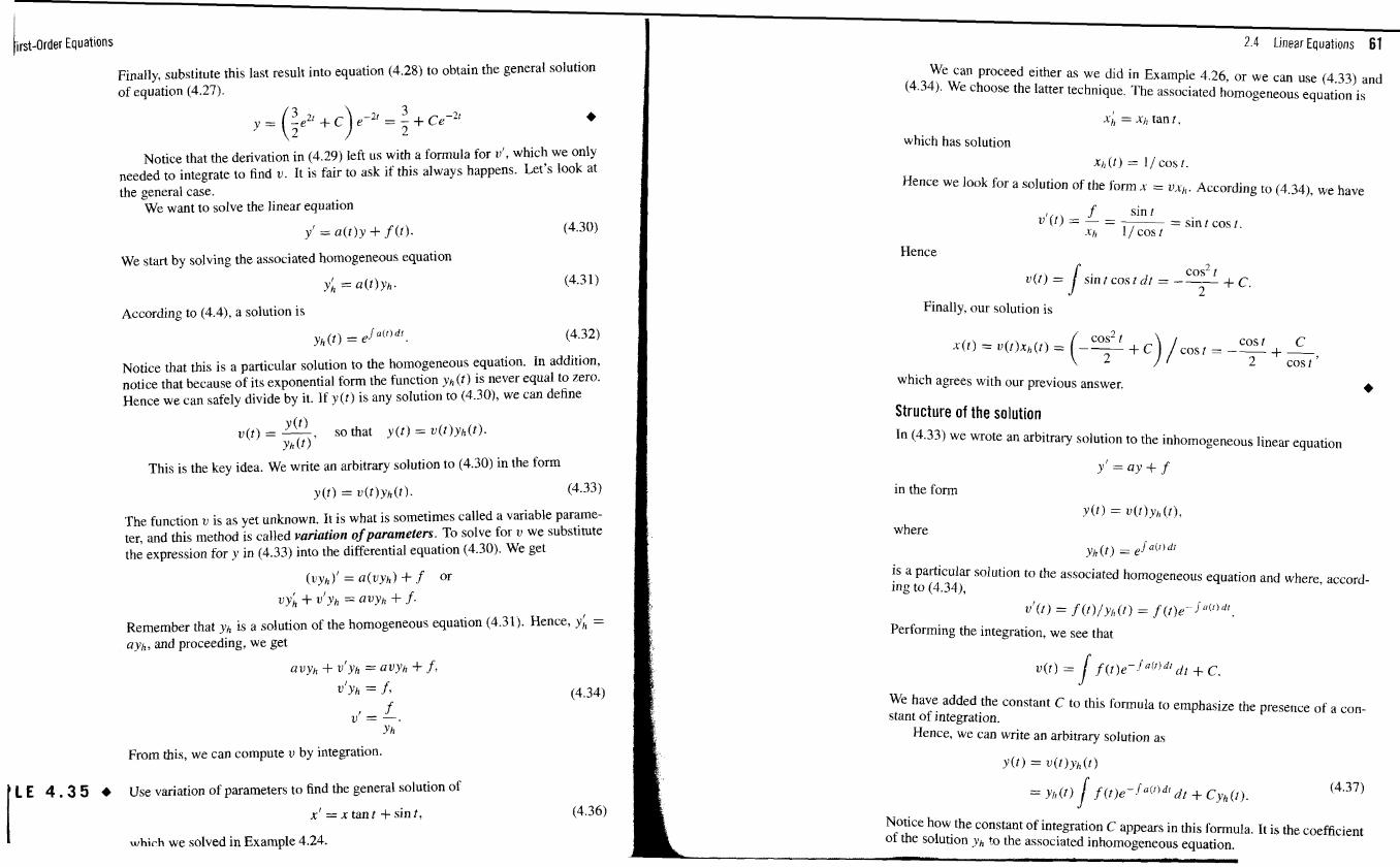
Finally, this last result into equation (4.28) to obtain the general We can proceed either as we did in Example 4.26, or we can use (4.33) and of equation (4.27). (4.34). We choose the latter technique. The associated homogeneous is
which has solution Notice that the denvation in (4.29) left US with a f0IXlllla for u', which we xh ( t ) = 1/ cos t.
needed to integrate to find IJ. It is fair to ask if this always happens- Letfs look at the general case. Hence we look for a solution of the form x = v.xh. According to (4.341, we have
We want to solve the linear equation f sin t ~ ' ( t ) = - = --- = sin t cos t .
y' = a ( t ) y + f (f). xh l / cos t
We start by solving the associated homogeneous equation Hence
y;, = a(t)yh.
According to (4 .4 , a solution is Finally. our solution is
~ ( t ) d t yh(t) = eJ . ~ ( t ) = u ( ~ ) x ~ ( t ) = --- cost C ( C0;21 + C ) / C O S I = -- + --,
ti^^ that this is a particular solution to the homogeneous equation. In addition, 2 cost notice that because of its exponential fonn the function yh ( t ) is never to which agrees with our previous answer. Hence we can safely divide by it. If p(t) is any ~0lUtion to (4.30), we can define
Structure of the solution ' ( ' ) so that y ( t ) = u(t)yh(t). v ( t ) = - yh ( t ) ' In (4.33) we wrote an arbitrary solution to the inhomogeneous linear equation
This is the key idea. We write an arbitrary ~ 0 l ~ t i o n to (4.30) in the form Y' = ay + f
y( t ) = u ( t ) ~ h ( t ) . in the form
The function is as yet unknown. It is what is sometimes called a variable parame- ~ ( t ) = IJ(t)y,,(t),
ter, and this method is called variation of parameters. To solve for 7~ we substitUte where
the expression for JJ in (4.33) into the differential equation (4.30). We get yh ( t ) e S ~ ( ' ) d t
( z I Y ~ ) ' a(vyh) + f Or is a particular solution to the associated homogeneous equation and where, accord- ing to (4.34),
vy;, + V ' Y ~ = avyh + f ' ~ ' ( t ) = f ( t ) / yh ( t ) = f ( t )e-JQ(')dt .
Remember that yh is a solution of the homogeneous equation (4.31). Y ; = Performing the integration, we see that ayh, and proceeding, we get
avyh + V ' Y ~ =avYh + f ~ u'yh = f,
f We have added the constant C to this formula to emphasize the presence of a con- IJ = -. stant of integration.
Y h Hence, we can write an arbitrary solution as From this, we can compute v by integration.
Y ( ~ I = V(t)) 'h( t)
E 4 . 3 5 6 Use variation of parameters to find the general solution of
X' = x tan t + sin t ,
which we solved in Example 4.24.
lirst-Order Equations
If we pick a particular solution y,,(r). i t will be associated with a ~anicular value of the constant C, say C,, so that
Comparing (4.37) and (4.38). we see that the difference of the two solutions to the inho~nogeneous equation is
Thus, the difference y - y,, is a constant multiple of y,, and is itself a solution to the homogeneous equation. Furthemore, if we set A = C - C,,, we see that an arbitrary solution y can be written as
Thus, we have demonstrated the following result, showing how the constant of in- tegration appears in the general solution to a linear equation. -
HEOREM 4.39 Suppose that y,, is a particular solution to the inhomogeneous equation
and that yh is a particular solution to the associated homogeneous equation. Then every solution to the inhomogeneous equation is of the form
y(t) = ?'/,(t) + Ayh(t), (4.40)
where A is an arbitrary constant. -
I In Exercises 1-12, find the general solution of each first-order, linear equation.
1. y 1 + y = 2 2. y' -3y = 5
3. y' + (2/x)y = (cos x)/x2 4. y' + 2ty = 5r
6. tx' = 4x + t -I 5. x' - 2x/(t + I) = (t + 112 2 5
7. ( I + x)yl + y = COSX 8. (1 + x"yl = 3x2y + x + x
9. L(di/dt) + Ri = E , L, R , E real constants
I 10. = my + clemx, m. cl real constants
11. y' = cosx - ysecx.
12. x' - (n/ t)x = ef tn , n a positive integer
13. (a) The differential equation y' + y cos r = cosx is linear. Use the technique of this section (integrating factor) to find the general solution.
(b) The equation y' + y c0s.r = cosx is also separable. Use the separation of variables technique to solve the equation and discuss any discrepancies (if any) between this solution and the solution found in part (a).
2.4 Linear Equations 63
In Exercises 14-17, find the solution of each initial value problem.
14. y' = y + 2xe2", y (0) = 3 15. (.u2 + l )y1+3xy = 6x, y(0) = -1 16. (1 + t2)y' + 4ty = (1 + t2)-2. y ( I ) = O 17. x' + x cos t = sin 2t, .r (0) = 1
In Exercises 18-21, find the solution of each initial value problem. Discuss the interval of existence and provide a sketch of your solution.
18. xy' + 2y = sin x , y (7712) = O
19. (2x + 3)y' = y + (2x + 3)'/', ))(-I) = 0 20. y l = c o s x - y s e c - r , y(O)= 1
21. ( 1 + t ) s l + s =cos t , x(-7712) = 0 22. The presence of nonlinear terms prevents us from using the technique of this
section. In special cases. a change of variable will transform the nonlinear equation into one that is linear. The equation known as Bernoulli's equation,
was proposed for solution by James Bernoulli in December 1695. In 1696, Leibniz pointed out that the equation can be reduced to a linear equation by taking XI-" as the dependent variable. Show that the change of variable, z = x ' ~ " . will transform the nonlinear Bernoulli equation into the linear equation
Hint: If z = XI-", then dz/dt = (dz/dx)(clx/dt) = (1 - n)x-"(d-rldt).
In Exercises 23-26, use the technique of Exercise 22 to transform the Bernoulli equation into a linear equation. Find the general solution of the resulting linear equation.
23. y' + x-'y = xy2 24. y' + Y = y2 25. xyl + y = x4y" 26. P' = aP - bp ' 27. The equation
where @, 4, and x are functions of t , is called the generalized Riccati equation. In general, the equation is not integrable by quadratures. However, suppose that one solution, say y = yl, is known.
(a) Show that the substitution y = + z reduces the generalized Riccati equa- tion to
dz - + (2y,@ + $12 + @z2 = 0, d t
which is an instance of Bernoulli's equation (see Exercise 22).
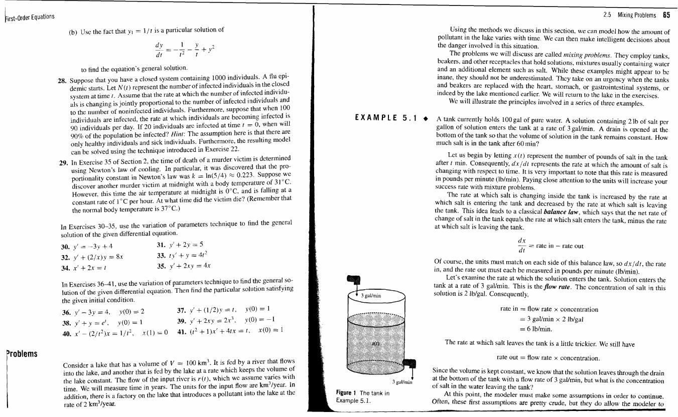
irst-Order Equations
(b) Use the fact that yl = l l t is a particular solution of
to find the equation's general solution.
28. Suppose that you have a closed system containing 1000 individuals. A flu epi- demic starts. Let N ( z ) represent the number of infected individuals in the closed system at time r . Assume that the rate at which the number of infected individu- als is changing is jointly proportional to the number of infected individuals and to the number of noninfected individuals Furthermore, suppose that when 100 individuals are infected, the rate at which individuals are becoming infected is 90 individuals per day. If 20 individuals arc infccted at time t = 0, when will 90% of the population be infected? Hint: The assumption here is that there are only healthy individuals and sick individuals. Furthermore, the resulting model can be solved using the technique introduced in Exercise 22.
29. In Exercise 35 of Section 2, the time of death of a murder victim is determined using Newton's law of cooling. In particular, it was discovered that the pro- portionality constant in Newton's law was k = ln(514) % 0.223 Suppose we discover another murder victim at midnight with a body temperature of 31°C. However, this time the air temperature at midnight is 0°C. and is falling at a constant rate of I "C per hour. At what time did the victim die? (Remember that the normal body temperature is 37°C.)
In Exercises 30-35. use the variation of parameters technique to find the general solution of the given differential equation.
30. y' = -3y + 4 31. y' + 2y = 5
32. y' + (2/x)y = 8x 33. tv' + y = 4t2
34. x' + 2x = t 35. JJ' + 2xy = 4x
In Exercises 3 6 4 1 , use the variation of parameters technique to find the general SO-
lution of the given differential equation. Then find the particular solution satisfying the given initial condition.
36. y' - 3y = 4. ~ ( 0 ) = 2 37. y 1 + ( 1 / 2 ) y = t , y (O)=I
38. y ' + y = e t , y ( O ) = l 39. + 2 . ~ ~ = 2 ~ ~ . ~ ( 0 ) = -1
40. x' - (2/r2)x = l / t 2 , x(1) = 0 41. (t2 + 1)x' + 4tx = t . x(0) = I
I roblems
Consider a lake that has a volume of V = 100 km3. It is fed by a river that flows into the lake, and another that is fed by the lake at a rate which keeps the volume of the lake constant. The flow of the input river is r ( t ) , which we assume varies with time. We will measure time in years. The units for the input flow are h3/year . In addition, there is a factory on the lake that introduces a pollutant into the lake at the rate of 2 km3/year.
2.5 Mixing Problems 65
Using the methods we discuss in this section, we can model how the amount of pollutant in the lake varies with time. We can then make intelligent decisions about the danger involved in this situation.
The problems we will discuss are called miking probleras. They employ tanks, beakers, and other receptacles that hold solutions, mixtures usually containing water and an additional element such as salt. While these examples might appear to be inane, they should not be underestimated. Thcy take on an urgency when the tanks and beakers are replaced with the heart, stomach, or gastrointestinal systems, or indeed by the lake mentioned earlier. We will return to the lake in the exercises.
We will illustrate the principles involved in a series of three examples.
E X A M P L E 5 . 1 + A tank currently holds 100 gal of pure water. A solution containing 2 lh of salt per gallon of solution enters the tank at a rate of 3 gal/min. A drain is opened at the bottom of the tank so that the volume of solution in the tank remains constant. How much salt is in the tank after 60 min?
Let us begin by letting x(t) represent the number of pounds of salt in the tank after t min. Consequently, dx/dt represents the rate at which the amount of salt is changing with respect to time. It is very important to note that this rate is measured in pounds per minute (lblmin). Paying close attention to the units will increase your success rate with mixture problems.
The rate at which salt is changing inside the tank is increased by the rate at which salt is entering the tank and decreased by the rate at which salt is leaving the tank. This idea leads to a classical balance law, which says that the net rate of change of salt in the tank equals the rate at which salt enters the tank, minus the rate at which salt is leaving the tank.
dx - = rate in - rate out dt
Of course, the units must match on each side of this balance law, so dxld t , the rate in, and the rate out must each be measured in pounds per minute (Iblmin).
Let's examine the rate at which the solution enters the tank. Solution enters the tank at a rate of 3 gallmin. This is theflow rate. The concentration of salt in this solution is 2 Ib/gal. Consequently,
rate in = flow rate x concentration
= 3 gal/min x 2 lb/gal
= 6 1 b/min.
The rate at which salt leaves the tank is a little trickier. We still have
rate out = flow rate x concentration.
Since the volume is kept constant, we know that the solution leaves through the drain " 4 at the bottom of the tank with a flow rate of 3 gal/rnin, but what is the concentration 3 gaVnliri
of salt in the water leaving the tank? Figure 1 The tank in At this point, the modeler must make some assumptions in order to continue. Example 5.1. Often, these first assumptions are pretty crude, but they do allow the modeler to
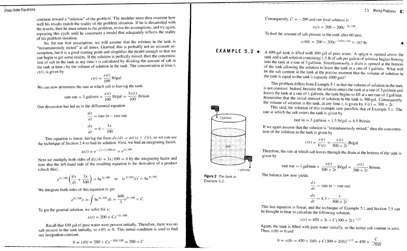
First-Order Equations
continue toward a "solution" of the problem. The modeler must then examine how well his results match the reality of the problem situation. If he is dissatisfied with the results, then he must return to the problem, revise his assumptions, and try again, repeating this cycle until he constructs a model that adequately reflects the reality of his problem situation.
So, for our first assumption, we will assume that the mixture in the tank is "instantaneously mixed" at all times. Granted, this is probably not an accurate as- sumption, but it is a good starting point and simplifies the model enough so that we can begin to get some results. If the solution is perfectly mixed, then the concentra- tion of salt in the tank at any time t is calculated by dividing the amount of salt in the tank at time r by the volume of solution in the tank. The concentration at time t , c ( t ) , is given by
We can now determine thc rate at which salt is leaving the tank.
( t ) 3 x ( t ) rate out = 3 gallmin x - lbtgal = --- lblmin 100 100
Our discussion has led us to the differential equation
d x - = rate in - rate out d t
d x - -
3 x = 6 - -.
dt 100
This equation is linear, having the for111 d x l d t = a ( t ) x + f ( I ) , SO we can use the technique of Section 2.4 to find its solution. First, we find an integrating factor,
Next we multiply both sides of dxlcit + 3x/100 = 6 by the integrating factor and note that the left-hand side of the resulting equation is the derivative of a product (check this).
We integrate both sides of this equation to get
e3r/100 600 = 1 6e3'/11"dr = -e3'/l" + (2.
3
To get the general solution, we solve for x:
x ( t ) = 200 + CU-""~O.
Recall that 100 gal of pure water were present initially. Therefore, there was no salt present in the tank initially, so x ( 0 ) = 0. This initial condition is used to find our integration constant.
0 = x(O) = 200 + ~ e - ~ ( ~ ) l ' ~ ~ = 200 + C .- -- -- - -
I 2.5 Mixing Problems 6;
E X A M P L E
Consequently, C = -200 and our final solution i 4
x ( r ) = 200 - 2 0 0 e ~ ~ ~ " ~ " .
To find the amount of salt present 111 the tank after 60 min,
x ( 6 0 ) = 200 - 200r -'("'/"'" % 167 lb.
A 600-gal tank is filled with 300 gal of pure water. A spigot is opened above the tank and a salt solution containing 1.5 Ib of salt per gallon of solution begins flowing into the tank at a rate of 3gallmin. Simultaneously, a drain is opened at the bottom of the tank allowing the solution to leave the tank at a rate of I gallmin. What will be the salt content in the tank at the precise moment that the volume of solution in the tank is equal to the tank's capacity (600 gal)?
This problem differs from Example 5.1 in that the volume of solution in the tank is not constant Indeed, because the solution enters the tank at a rate of 3 gallmin and leaves the tank at a rate of 1 gallmin, the tank begins to fill at a net rate of 2 gallmin. Remember that the initial amount of solution in the tank is 300 gal. Consequently, the volume of solution in the tank, at any time t , is given by V ( r ) = 300 t 2t.
This said, the solution of this example now parallels that of Example 5 . 1 The rate at which the salt enters the tank is given by
rate in = 3 gaVmin x 1.5 Iblgal = 4.5 Iblmin.
If we again assume that the solution is "instantaneously mixed," then the concentra- tion of the solution in the tank is given by
~ ( 0 - c ( t ) = - - Iblgal.
V ( t ) 300 + 2t Therefore, the rate at which salt leaves through the drain at the bottom of the tank is given by
rate out = 1 gallmin x x ( r ) Iblgal =
300 + 2t X ( t )
Iblmin. 300 + 2t
Figure 2 The tank rn The balance law now yields
Example 5.2. d x - = rate in - rate out, dt
This last equation is linear, and the technique of Example 5.1 and Section 2.5 can be brought to bear to calculate the following solution.
Again, the tank is filled with pure water initially, so the initial salt content is zero. Thus, ~ ( 0 ) = 0 and
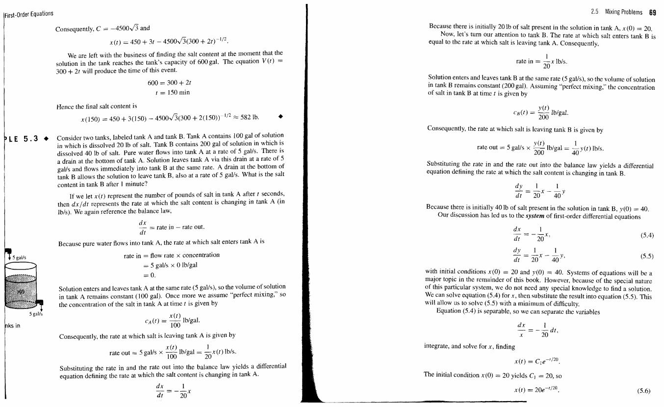
Ififst-Order Equations 2.5 Mixing Problems 69
I Consequently, C = - 4 5 0 0 a and
We are left with the business of finding the salt content at the moment that the solution in the tank reaches the tank's capacity of 600 gal. The equation V ( t ) = 300 + 2t will produce the time of this event.
600 = 300 + 2t t = 150 min
1 Hence the final salt content is
) L E 5 . 3 4 Consider two tanks, labeled tank A and tank B. Tank A contains 100 gal of solution in which is dissolved 20 lb of salt. Tank B contains 200 gal of solution in which is dissolved 40 Ib of salt. Pure water flows into tank A at a rate of 5 gaVs. There is a drain at the bottom of tank A. Solution leaves tank A via this drain at a rate of 5 gays and flows immediately into tank B at the same rate. A drain at the bottom of tank B allows the solution to leave tank B, also at a rate of 5 gal/s. What is the salt content in tank B after 1 minute?
If we let x(t) represent the number of pounds of salt in tank A after t seconds, then dx ld t represents the rate at which the salt content is changing in tank A (in lbls). We again reference the balance law,
nx - = rate in - rate out. dt
Because pure water flows into tank A, the rate at which salt enters tank A is
5 gaVs b rate in = flow rate x concentration = 5 gaVs x 0 lblgal
= 0.
Solution enters and leaves tank A at the same rate (5 galls), so the volume of solution in tank A remains constant (100 gal). Once more we assume "perfect mixing," so the concentration of the salt in tank A at time t is given by
x(t> CA (t) = - lblgal.
100
I Consequently, the rate at which salt is leaving tank A is given by
x( t> 1 rate out = 5 gays x --- lblgal = -x(t) lbls.
100 20
Substituting the rate in and the rate out into the balance law yields a differential equation defining the rate at which the salt content is changing in tank A.
Because there is initially 20 Ib of salt present in the solution in tank A, x(0) = 20. Now, let's turn our attention to tank B. The rate at which salt enters tank B is
equal to the rate at which salt is leaving tank A. Consequently,
1 rate in = -x lbls.
20
Solution enters and leaves tank B at the same rate (5 gaVs), so the volume of solution in tank B remains constant (200 gal). Assuming "perfect mixing," the concentration of salt in tank B at time t is given by
Consequently, the rate at which salt is leaving tank B is given by
v(t> 1 rate out = 5 galls x I-- Iblgal = - y (t) lbls. 200 40
Substituting the rate in and the rate out into the balance law yields a differential equation defining the rate at which the salt content is changing in tank B.
Because there is initially 40 lb of salt present in the solution in tank B, y (0) = 40. Our discussion has led us to the system of first-order differential equations
with initial conditions x(0) = 20 and y(0) = 40. Systems of equations will be a major topic in the remainder of this book. However, because of the special nature of this particular system, we do not need any special knowledge to find a solution. We can solve equation (5.4) for x, then substitute the result into equation (5.5). This will allow us to solve (5.5) with a minimum of difficulty.
Equation (5.4) is separable, so we can separate the variables
integrate, and solve for x, finding
The initial condition x(0) = 20 yields C1 = 20, so
x ( t ) = 20e-'Iz0.
We now substitute equation (5.6) into equation (5.5) and simplify to obtain the equation
This equation is linear, and u ( t ) = et/" is an integrating factor. Multiplying both sides of equation (5.7) by u , we get
lntegrating and solving for Y, we get
et/40y = -40e-'/~' + C2 or
y(t) = -40c-'/~' + ~ ~ e - ~ / ~ ~ ' .
The initial condition y (0) = 40 yields C2 = 80 and
y (t) -40e-'/~' + 80e~ ' /~ ' .
Finally, we can use equation (5.8) to find the salt content in tank B at t = 1 min = 60 seconds, finding that
~1(60) = -40e-("O'l'' + 80e-'~''" % 15.9 1b.
................ EXERCISES 1. A tank contains 100 gal of pure water. At time zero, a sugar-water solution
containing 0.2 lb of sugar per gallon enters the tank at a rate of 3 gal per minute. Simultaneously, a drain is opened at the bottom of the tank allowing the sugar- solution to leave the tank at 3 gal per minute. Assume that the solution in the tank is kept perfectly mixed at all times.
(a) What will be the sugar content in the tank after 20 minutes?
(b) How long will it take the sugar content in the tank to reach 15 Ib?
(c) What will be the eventual sugar content in the tank?
2. A tank initially contains 50 gal of sugar water having a concentration of 2 lb of sugar for each gallon of water. At time zero, pure water begins pouring into the tank at a rate of 2 gal per minute. Simultaneously, a drain is opened at the bottom of the tank so that the volume of the sugar-water solution in the tank remains constant.
(a) How much sugar is in the tank after 10 minutes?
(b) How long will it take the sugar content in the tank to dip below 20 lb? \ , -
(c) What will be the eventual sugar content in the tank?
3. A tank initially contains 100 gal of water in which is dissolved 2 lb of salt. A salt-water solution containing 1 lb of salt for every 4 gal of solution enters the tank at a rate of 5 gal per minute. Solution leaves the tank at the same rate, allowing for a constant solution volume in the tank.
2.5 M~xing Problems 71
(a) Use an analytic method to determine the eventual salt content in the tank.
(b) Use a numerical solver to determine the eventual salt content in the tank and compare your approximation with the analytical solution found in part (a).
4. A tank contains 500 gal of a salt-water solution containing 0.05 lb of salt per gallon of water. Pure water is poured into the tank and a drain at the bottom of the tank is adjusted so as to keep the volume of solution in the tank constant. At what rate (gallmin) should the water be poured into the tank to lower the salt concentration to 0.01 lblgal of water in under one hour?
5. A 50 gal tank initially contains 20 gal of pure water. Salt-water solution con- taining 0.5 lb of salt for each gallon of water begins entering the tank at a rate of 4 gallmin. Simultaneously, a drain is opened at the bottom of the tank, allowing the salt-water solution to leave the tank at a rate of 2 gallmin. What is the salt content (lb) in the tank at the precise moment that the tank is full of salt-water solution?
6. A tank initially contains 100 gal of a salt-water solution containing 0.05 Ib of salt for each gallon of water. At time zero, pure water is poured into the tank at a rate of 2 gal per minute. Simultaneously, a drain is opened at the bottom of the tank that allows salt-water solution to leave the tank at a rate of 3 gal per minute. What will be the salt content in the tank when precisely 50 gal of salt solution remain?
7. A tank initially contains 100 gal of pure water. Water begins entering a tank via two pipes: through pipe A at 6 gal per minute. and pipe B at 4 gal per minute. Simultaneously, a drain is opened at the bottom of the tank through which solution leaves the tank at a rate of 8 gal per minute.
(a) To their dismay, supervisors discover that the water coming into the tank through pipe A is contaminated, containing 0.5 lb of pollutant per gallon of water. If the process had been running undetected for I0 minutes, how much pollutant is in the tank at the end of this 10-minute period?
(b) The supervisors correct their error and shut down pipe A, allowing pipe B and the drain to function in precisely the same manner as they did before the contaminant was discovered in pipe A. How long will it take the pollutant in the tank to reach one half of the level achieved in part (a)?
8. Suppose that a solution containing a drug enters a bodily organ at the rate a cm"/s, with drug concentration K glcm". Solution leaves the organ at a slower rate of b cmqs. Further. the faster rate of infusion causes the organ's volume to increase with time according to V(t) = Vo + r t , with Vo its initial volume. If there is no initial quantity of the drug in the organ, show that the concentration of the drug in the organ is given by
9. A lake, with volume V = 100 km3, is fed by a river at a rate of r km31yr. In addition, there is a factory on the lake that introduces a pollutant into the lake at the rate of p km3/yr. There is another river that is fed by the lake at a rate which
/ ~ i rs t -Order Equations
keeps the volume of the lake constant. This means that the rate of flow from the lake into the outlet river is (p + r ) km31yr. Let x(t) denote the volume of the pollutant in the lake at time t, and let c(t) = x(t) /V denote the concentration of the pollutant.
(a) Show that, under the assumption of immediate and perfect mixing of the pollutant into the lake water, the concentration satisfies the differential equation
(b) It has been determined that a concentration of over 2% is hazardous for the fish in the lake. Suppose that r = 50 krdlyr, p = 2 km31yr, and the initial concentration of pollutant in the lake is zero. How long will it take the lake to become hazardous to the health of the fish?
10. Suppose that the factory in Exercise 9 stops operating at time t = 0 and that the concentration of pollutant in the lake was 3.5% at the time. Approximately how long will it take before the concentration falls below 2%, and the lake is no longer hazardous for the fish?
11. Rivers do not flow at the same rate year-around. They tend to be full in the spring when the snow melts, and to flow more slowly in the fall. TO take this into account, suppose the flow of the input river in Exercise 9 is
Our river flows at its maximum rate one-third into the year (i.e., around the first of April) and at its minimum around the first of October.
(a) Setting p = 2, and using this flow rate, use your numerical solver to plot the concentration for several choices of initial concentration between 0% and 4%. (You might have to reduce the relative error tolerance of your solver, perhaps to 5 x 10-12.) How would you describe the behavior of the concentration for large values of time?
(b) It might be expected that after settling into a steady state, the concentra- tion would be greatest when the flow was smallest (i.e., around the first of October). At what time of year does it actually occur?
12. Consider two tanks, labeled tank A and tank B for reference. Tank A contains 100 gal of solution in which is dissolved 20 lb of salt. Tank B contains 200 gal of solution in which is dissolved 40 lb of salt. Pure water flows into tank A at a rate of 5 galls. There is a drain at the bottom of tank A. Solution leaves tank A via this drain at a rate of 5 galls and flows immediately into tank B at the same rate. A drain at the bottom of tank B allows the solution to leave tank B at a rate of 2.5 galls. What is the salt content in tank B at the precise moment that tank B contains 250 gal of solution?
13. Lake Happy Times contains 100 km3 of pure water. It is fed by a river at a rate of 50 km31yr. At time zero, there is a factory on one shore of Lake Happy Times that begins introducing a pollutant to the lake at a rate of 2 km3Iyr. There is another river that is fed by Lake Happy Times at a rate which keeps the volume of Lake Happy Times constant. This means that the rate of flow from
2.6 Exact Differential Equations 73
Lake Happy Times into the outlet river is 52 km31yr. In turn, the flow from this outlet river goes into another lake, Lake Sad Times, at an equal rate. Finally, Lake Sad Times feeds another outlet river at a rate that keeps the volume of Lake Sad Times at a constant 100 km3.
(a) Find the amount of pollutant in Lake Sad Times at the end of 3 months.
(b) At the end of 3 months, observers close the factory due to environmental concerns and no further pollutant enters Lake Happy Times. How long will it take for the pollutant in Lake Sad Times (found in part (a)) to be cut in half? Hint: Plot the solution of pollutant versus time for positive time.
14. Two tanks, tank 1 and tank 11, are filled with V gal of pure water. A solution containing a lb of salt per gallon of water is poured into tank I at a rate of b gal per minute. The solution leaves tank I at a rate of b gallmin and enters tank 11 at the same rate (b gallmin). A drain is adjusted on tank I1 and solution leaves tank I1 at a rate of b gallmin. This keeps the volume of solution constant in both tanks (V gal). Show that the amount of salt solution in tank 11, as a function of time t, is given by a V - ~ b t e - ( ~ / " ) ~ - a ~e-(~!") ' .
2.6 Exact Differential Equations In this section, we will consider differential equations that can be written as
dy P(x, y) + Q(x, y)- = 0, dx (6.1)
where P and Q are functions of both the independent variable x and the dependent variable y. This is a very general class of differential equations. As usual, a so- lution will be a differentiable function y ( ~ ) defined for x in an interval, such that equation (6.1) is satisfied at each point in the interval.
E X A M P L E 6 . 2 + The differential equation
has the function y(x) = as a solution on the whole real line. This can be verified by direct computation, since y'(x) = -.xe--'Li2 = -xy. + Differential forms and differential equations It will be convenient when dealing with differential equations of the generality cov- ered by equation (6.1) to use the language of differential forms. A differential form in the two variables x and y is an expression of the type
where P and Q are functions of x and y. The simple forms dx and dy are called differentials.
Suppose that Y = y(x). Then dy = y1(x) dx. If we substitute this into the differential form w in (6.3), we get
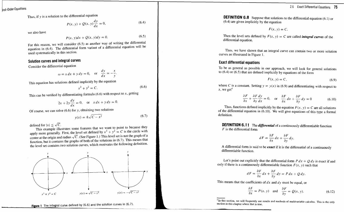
lrst-0rder Equations I Thus, if y is a solution to the differential equation
we also have
P ( x , y ) d x + Q ( x , y )dy = 0. (6.5)
For this reason, we will consider (6.5) as another way of writing the differential equation in (6.4). The differential form variant of a differential equation will be used systematically in this section.
Solution curves and integral curves Consider the differential equation
This equation has solutions defined implicitly by the equation x 2 + y2 = C . (6.6)
This can be verified by differentiating formula (6.6) with respect to x , getting
Of course, we can solve (6.6) for y , obtaining two solutions
defined for ( x ( 5 z. This example illustrates some features that we want to point to because they
apply more generally. First, the level set defined by x 2 + y2 = C is the circle with center at the origin and radius z. (See Figure I ) This level set is not the graph of a function, but it contains the graphs of both of the solutions in (6.7). This means that the level set contains two solution curves, which motivates the following definition.
Figure 1 The integral curve defined by (6.6) and the solution curves in (6.7). , ' . . - -
2.6 Exact Differential Equations 75
DEFINITION 6.8 Suppose that solutions to the differential equation (6.1) or (6.4) are given implicitly by the equation
Then the level sets defined by F ( x , y ) = C are called integral curves of the differential equation.
Thus, we have shown that an integral curve can contain two or more solution curves as illustrated in Figure 1.
Exact differential equations To be as general as possible in our approach, we will look for general solutions to (6.4) or (6.5) that are defined implicitly by equations of the form
where C is a constant. Setting y = y ( x ) in (6.9) and differentiating with respect to x , we get4
Thus, functions defined implicitly by the equation F ( x , y ) = C are all solutions of the differential equation in (6.10). We will give equations of this type a formal definition.
DEFINITION 6.1 1 The diflerential of a continuously differentiable function F is the differential form
A differential form is said to be exact if it is the differential of a continuously differentiable function.
Let's point out explicitly that the differential form P d x + Q d y is exact if and only if there is a continuously differentiable function F ( x , y ) such that
a F a F d F = - d x + - d y = P d x + Q d y .
ax ay
This means that the coefficients of d x and d y must be equal, or
a F a F - = P ( x , y ) and - = Q ( x , y ) . ax ay
41n this section, we will frequently use results and methods of multivariable calculus. This is the only section in this chapter where that is true.
)&order Equations
E 6 . 1 3 4 Solve the equation 2x dx + 4y3 dy = 0. Because the variables are separated in the equation, it is not difficult to discover
that
Consequently, the differential form 2x dx + 4y3 dy is exact. Furthermore, the gen- eral solution to the equation 2x d r + 4y3 dy = 0 is given by
Example 6.13 illustrates that it is quite easy to solve an exact differential equa- tion. However, two questions come to mind.
I. Given a differential form w = P dx + Q dy, how do we know if it is exact?
2. If a differential form is exact, is there an easy way to find F such that d F = P d x + Qdy?
Both of these questions are answered in the next result.
w--
Let w = P dx + Q dy be a differential form where both P and Q are continuously I-- differentiable.
(a) If w is exact, then
in a rectangle R , then w is exact in R. More precisely, o = d~ in R , where F (x . y ) is defined for (x, y ) in R by the formula
and @ satisfies
Proof To prove (a), suppose that w = d F . Then
a F aF - = P and -- - Q . ax a y
Both P and Q are continuously differentiable. so F is twice continuously differen- tiable. This means that the mixed second-order derivatives of F are equal. Conse- quently,
2.6 Exact Differential E ~ u a t i o n s 77
To prove (b), we need to find a function F satisfying both equations in (6.17). If we integrate the equation a F l ax = P , then by the fundamental theorem of calculus, we must have
F(x, Y) = P(x, Y) dx + @(y), S where 4 is a function of y only. This is equation (6.15). In this formula 1 P(x , y) dx represents a particular indefinite integral, and @(y) represents the constant of inte- gration. Since we are integrating with respect to x, this "constant" can still depend on y.
To discover what @ is, we differentiate F as given in (6.15) with respect to y
The second formula in (6.17) says that a F l ay = Q, so we see that @ must satisfy
This is equation (6.16), and it can be solved by integration provided that the function on the right does not depend on the variable x. The hypothesis of our theorem guarantees that this is true. To see this, it suffices to show that the derivative of the function on the right with respect to x is zero. We have
The statement of Theorem 6.14 gives us a method for solving exact equations. Let's look at an example.
E X A M P 1 E 6 . 1 8 4 Show that the equation eY dx + (xey - sin y) dg = 0 is exact and find a general solution.
Since
we know the equation is exact. To find a general solution, we need to find a function F(x, y ) such that
aF aF - = eY and - = xeY - sin y . ax ay
I 2.6 Exact Differential Equations 79 1irst-Order Equations
We solve the first equation by integrating, getting
Differeiaiating with respect to y , and using that a f /ay = xe' - sin Y , we get
xe' - sin y = r e ' + 4 ' ( y ) .
Therefore. d l ( y ) = - sin x. which has solution 4 ( y ) = COS y. Finally. F(-r. .?') = + cosy, and solutioils are given implicitly by
E 6 . 1 9 4 l a the equation -?. dx + x d y = 0 exact?
In this case, P ( x . x ) = - y and Q ( X , y ) = x . Hence
a p a Q - = -1 and - = 1, n y ax
I Since these are not equal, the equation is not exact. 4
Solutions and integrating factors NOW let's look at a differential equation
P ( x . y ) dx + Q(.r. y ) dx = 0.
which niay or may not be exact. Again we will look for general solutions that are defined implicitly by equations of the form
where C is a constant. Suppose y = f i x ) is defined by (6.21). Differentiating (6.21) with respect to
.r, we get
i3F aF d y tly - -- a F / a x ; I , + ~ Z = O ~ Or -- d x a F / a y
On the other hand, notice that if y ( x ) is a solution to (6.20), we have
Comparing (6.23) with (6.22). we see that y is a solution provided that
If we let p = p ( x , y ) be defined as this common factor, we have
a F a F - = p P and - - a x a y - PQ.
Then
This shows that pw is exact. Let's make a definition.
DEFINITION 6.25 An integrating factor for the differential equation w = P d.u + Q d y = O is a function p ( x , y ) such that the form p(r., = p ( x , y ) P ( x , y ) d x + M x , .y)Q(x, y ) d y is exact.
We have shown that every differential equation for which there is a general solution of the form F ( x , y ) = C has an integrating factor. This suggests a strategy for finding a general solution to a differential equation
1. Find an integrating factor p , so that pP d x + W Q d v is exact.
2. Find a function F such that d F = p P d x + p Q d y .
Then a general solution is given implicitly by F ( x , y ) = C
E X A M P L E 6 . 2 6 + Consider the equation ( x + y ) d x - x d y = 0. Show that the equation is not exact and that 1 / x 2 is an integrating factor. Find a general solution.
Since
the equation is not exact. On the other hand, after we multiply the equation by 1 / x 2 , we get the equation
( x + y ) d x d y -- = 0. x 2 X
For this equation. we have
so the equation is exact and 1 / x 2 is an integrating factor. To solve it, we set
To find 4 , we differentiate this with respect to y , using the fact that a F l a y = - l l x . We get
This can be easily solved for y , so we write Our ~olufion as
y(x) = x ln 1x1 - C x .
We will exploit this strategy in what follows. It is reassuring to know that integrating factors always exist, but as we will see, it is not always easy to find one. Even in Example 6.26, the choice of l / x 2 is not at all obvious.
Separable equations A differential equation of the form
P ( x ) dx + Q ( Y ) dy = 0
is said to have its variables separated. The coefficient P depends only on x , so we have a P/By = 0. For the same reason a Q /ax = 0. Thus we see that any equation with separated variables is exact. Therefore, by Theorem 6.14, the solution is given implicitly by the equation F (x , y ) = C, where
and
Hence $ ( y ) = Q ( y ) dy and
A differential equation is said to be separable if there is an integrating factor that will separate the variables. Most important are equations of the type
In differential notation, t h s becomes
Multiplication by the integrating factor q ( y ) yields
... ~ ; , - h has its variables separated.
E X A M P L E 6 .2 8 4 Solve the equation -
2.6 Exact Differential Equations 81
In Example 6.19, we showed that the differential equation -g d x f x dy = 0 is not exact. However, this equation is separable. If we multiply this equation by I / xy , we get
Consequently, we can write down the solution using (6.27). To avoid problems with division by zero, we must stay away from where x = 0 or y = 0. Let's stay in the first quadrant where both x and y are positive. Then (6.27) becomes
Thus, our general solution is I n ( y / x ) = C. This can be written more conveniently by exponentiating. Then with A = eC
we get y = Ax as our general solution. Of course, this solution is only valid where both .x and y are positive, but we can redo the analysis in each quadrant and we get the same formula. Hence y = A x is indeed the general formula, and the solution curves are simply the straight half-lines through the origin. 4
Separable equations are dealt with in some detail in Section 2.2, so we will not spend any more time on them here.
Finding integrating factors Although an integrating factor exists whenever there is a general solution, this fact and its proof do not give us any insight into finding an integrating factor. In fact, there is no general procedure for finding integrating factors. Finding them is a genuine mathematical art.
One general way to search for an integrating factor starts from the criterion for exactness that we found in Theorem 6.14. Suppose u = P d x + Q dy and we want to find p such that pu = p P dx + p Q dy is exact. According to Theorem 6.14, p must satisfy
This is a partial differential equation for p. However, we only need to find one solution, and sometimes we can make assumptions about ,u that make this equation simpler. Here's an example where this process is successful.
E X A M P L E 6 . 3 1 4 Solve the equation (xy - 2) dx + (x2 - x y ) dy = 0.
In this case, a Play = x and a Q/ax = 2x - y, so the equation is not exact. Multiply both sides of the equation by an undetermined integrating factor.
p(xy - 2) dx + p(x2 - xy) dy = 0
I1 o
lr
3
El?
o
first-Order Equations
Homogeneous equations A function G(x, y) is homogeneous of degree n if
G(tx, ty) = tnG(x, y)
for all t > 0 and all x # 0 and y # 0. Thus the functions
I l n ( x ) 2x3 - 3x2y + 2xy2 - y3, and
x2 + v2 '
are homogeneous of degrees -2,0,3, and 1, respectively. The functions
x + x y , sin(x). l n ( x + y + l ) . and x - y - 2
are not homogeneous. A differential equation
P d x + Q d y = O
is said to be homogeneous5 if both of the coefficients P and Q are homogeneous of the same degree. Homogeneous equations can be put into a form in which they can be solved by using the substitution y = XU, where u is a new variable. Let's look at an example first and then we will examine the general case.
L E 6 . 3 5 + Verify that (x2 + y2) dx + xy dy = 0 is homogeneous and find a solution.
Both x2 + y2 and xy are homogeneous of degree 2. so the equation is ho- mogeneous. To solve the equation, we make the substitution y = xu. Then d Y = u dx + x du, so the equation becomes
I (x2 + x2u2) d~ + X ~ U ( L ~ dx + x du) = 0.
After canceling out the common factor x2 and collecting terms, this becomes
(1 + 2v2) dx + xu dv = 0.
Although this is not immediately solvable, it is separable. The integrating factor I
transforms the equation into the equation dx vdv - +-=o. x 1 + 2v2
Integrating, we get l n ~ x l + In( l+ 2 7 ~ ~ ) " ~ = k ,
where k is a constant. If we multiply by 4 and exponentiate, this becomes
x4(1 +2v2) = e4k = C .
Substituting v = y/x, we get our final answer x4 + 2x2y2 = C.
- We have used the term homogeneous differential equation with a completely different meaning in Sec-
tion 2.4. Unfortunately. both usages have become standard. The meanings are sufficiently different that you should not have any difficulty, but keep your eyes open.
2.6 Exact Differential Equations 85
In working this example, we did two things. First we made the substitution y = xu, and then we looked for an integrating factor that will separate the variables. These two steps will serve to find the solution for any homogeneous equation. To see this, let's start with
where P and Q are both homogeneous of degree n. We make the substitution y = xu, and we get
P(x, X U ) dx + Q(x, xu) (vd.r + x du) = 0.
The homogeneity means that P(x.xu) = x n P ( l . o) and Q(x, xu) = x U Q ( l , u). Using this, dividing out the common term x" , and collecting terms, our differential equation becomes
(P(1, v) + uQ(1. u)) dx + xQcl, u) dv = 0.
We recognize that the integrating factor
x(P(1, v) + vQ(1. u>>
will separate the variables, leaving us with the equation
This equation has separated variabIes, so it can be solved. Finally. we substitute u = v/x to put the answer in terms of the original variables. This verifies that the method works in general. However, when working problems of this type, it is usually better to make the substitution y = ux and then compute with the result, rather than remember the formula in (6.36).
................ EXERCISES In Exercises 1-8, calculate the total differential d F for the given function F.
In Exercises 9-21, determine which of the equations are exact and solve the ones that are.
9. (2x + y) dx + (X - 6y) dy = 0
10. (1 - y sinx) dx + (cosx) dy = 0
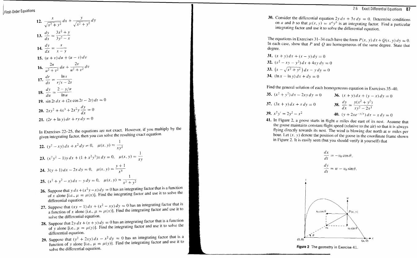
In Exercises 22-25. the equations are not exact. However, if you multiply by the given integrating factor, then you can solve the resulting exact equation.
y 4 - 1 24. 3 ( y + l ) d x - 2 x d y = O , @ ( x , y ) = - x4
1 25. ( ,x2+y2 - x ) d x - y d y = 0, @(s, y ) = -
x2 + .Y2
26. Suppose that y dx + (x2 y - x ) dy = 0 has an integrating factor that is a function of x alone [i.e., p = ~ ( x ) ] . Find the integrating factor and use it to solve the differential equation.
27. Suppose that ( x y - 1) dx + (x2 - x y ) dy = 0 has an integrating factor that is a function of x alone [i.e., p = ~ ( x ) ] . Find the integrating factor and use it to solve the differential equation.
28. Suppose that 2v dx + ( x + y ) dy = 0 has an integrating factor that is a function of y alone [i.e., p = ~ ( g ) ] . Find the integrating factor and use it to solve the differential equation. --
29. Suppose that (y2 + 2xy) dx - x2 dy = 0 has an integrating factor that is a function of y alone [i.e., P = p ( y ) ] . Find the integrating factor and use it to solve the differential equation.
30. Consider the differential equation 2y d a + 3.x dy = 0. Determine conditions on n and b so that p ( x , v ) = x0y" is an integrating factor. Find a particular integrating factor and use it to solve the differential equation.
The equations in Exercises 31-34 each have the form P(x , y ) dx + Q ( u , y ) dv = 0. In each case, show that P and Q are homogeneous of the same degree. State that degree.
32. ( x2 - xy - y 2 ) d x + 4xy dy = 0
33. ( x - J m ) d x - y d y = O
34. ( I n x - I n y ) d x + d y = O
Find the general solution of each homogeneous equation in Exercises 35-40,
35. ( x2 + v 2 ) rix - 2xy dy = 0 36. (x + y ) d x + ( y - x ) d y = 0
nv y(.r2 + y2 ) 37. (3x + y ) d x + .x dy = 0 38. - = d x zy2 - 2x3
39. x2 y' = 2y2 - x2 40. ( v + 2xe-HX) dx - x dy = 0 41. In Figure 2, a goose starts in flight u miles due east of its nest. Assume that
the goose maintains constant flight speed (relative to the air) so that it is always flying directly towards its nest. The wind is blowing due north at ul miles per hour. Let ( x , .Y) denote the position of the goose in the coordinate frame shown in Figure 2. It is easily seen (but you should verify it yourself) that
- = w - vo sin 0. d t
Figure 2 The geometry in Exercise 41.
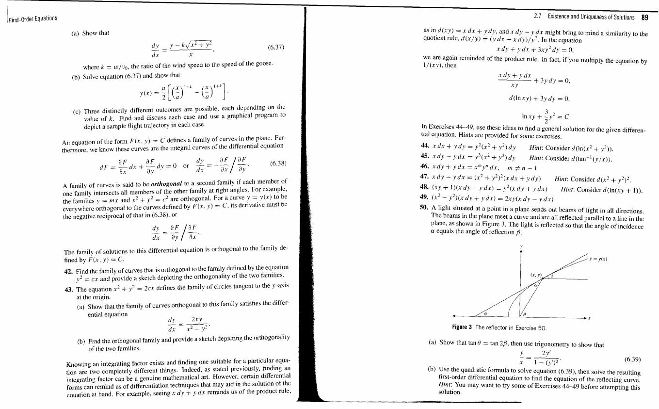
~irst-Order Equations
(a) Show that
where k = w/uO, the ratio of the wind speed to the speed of the goose.
(b) Solve equation (6.37) and show that
(c) Three distinctly different outcomes are possible, each depending on the value of k. Find and discuss each case and use a graphical program to depict a sample flight trajectory in each case.
An equation of the form F ( r , y ) = C defines a family of curves in the plane. Fur- thermore, we know these curves are the integral curves of the differential equation
A family of curves is said to be orthogonal to a second family if each member of one family intersects all members of the other family at right angles. For example, the families y = rnx and x 2 + y2 = c2 are orthogonal. For a curve y = y ( x ) to be everywhere orthogonal to the curves defined by F ( x , )I) = C. its derivative must be the negative reciprocal of that in (6.38), or
The family of solutions to this differential equation is orthogonal to the family de- fined by F ( x , y ) = C.
42. Find the family of curves that is orthogonal to the family defined by the equation y2 = c x and provide a sketch depicting the orthogonality of the two families.
43. The equation x 2 + y2 = 2cx defines the family of circles tangent to the y-axis at the origin.
(a) Show that the family of curves orthogonal to this family satisfies the differ- ential equation
d j j - 2.ry - - d x m.
( b ) Find the orthogonal family and provide a sketch depicting the orthogonality of the two families.
Knowing an integrating factor exists and finding one suitable for a particular equa- tion are two completely different things. Indeed, as stated previously, finding an integrating factor can be a genuine mathematical art. However, certain differential forms can remind us of differentiation techniques that may aid in the solution of the eauation at hand. For example, seeing .u d y + y d s reminds us of the product rule,
as in d ( x y ) = x d x + y d y , and x d y - v d x might bring to mind a similarity to the quotient rule, d ( x / y ) = ( y d x - x d y ) / y 2 . In the equation
x d y + y d x + 3 x . ~ ~ d ~ = 0 , we are again reminded of the product rule. In fact, if you multiply the equation by 1 / ( x p) , then
L In Exercises 44-49, use these ideas to find a general solution for the given differen- tial equation. Hints are provided for some exercises.
44. x d.r + y d y = y2(x2 + y2) d y Hint: Consider d( ln ( r2 + Y ~ ) ) . 45. x d y - y d r = y 3 ( x 2 + y2) d y Hint: Consider d(tanp' ( y l r ) ) . 46. x d y + y d x = xmy"d.r, rn # n - 1 47- x d ~ - Y d x = ( x 2 + y2)'(x d x + y d g ) Hint: Consider d ( x 2 + J I ' ) ~ .
48- ( x y + l ) ( x d . ~ - .Y d x ) = y 2 ( x d y + y d x ) Hint: Consider d(ln(.rv + 1)). 49. (s2 - y 2 ) ( x d y + y d x ) = 2.ry(x d y - y d x )
50. A light situated at a point in a plane sends out beams of light in all directions. The beams in the plane meet a curve and are all reflected parallel to a line in the plane, as shown in Figure 3. The light is reflected so that the angle of incidence a equals the angle of reflection ,6.
Figure 3 The reflector in Exercise 50.
(a) Show that tan 8 = tan 28, then use trigonometry to show that
Y - - - 2yr x 1 - ( y o 2 . (6.39)
(b) Use the quadratic formula to solve equation (6.39), then solve the resulting first-order differential equation to find the equation of the reflecting curve. Hint: You may want to try some of Exercises 4 4 4 9 before attempting this solution.
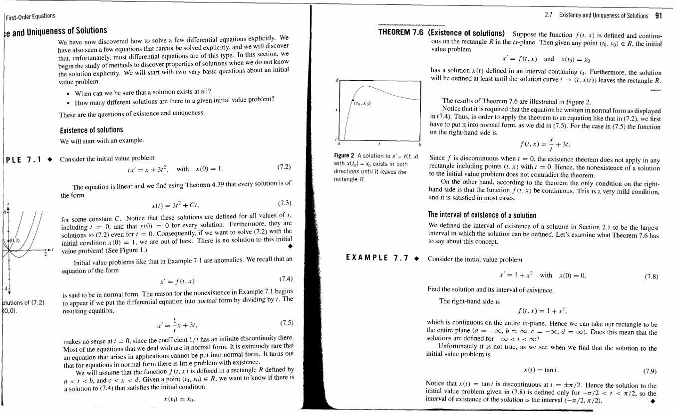
I First-Order Equations
;e and Uniqueness of Solutions We have now discovered how to solve a few differential equations explicitly. We have also seen a few equations that cannot be solved explicitly, and we will discover that, unfortunately, most differential equations are of this type. In this section, we begin the study of methods to discover properties of solutions when we do not know the solution explicitly. We will start with two very basic questions about an initial value problem.
When can we be sure that a solution exists at all?
How many different solutions are there to a given initial value problem?
These are the questions of existence and uniqueness.
Existence of solutions We will start with an example.
p L E 7 . 1 + Consider the initial value problem
tx' = x + 3t2, with x(0) = 1.
The equation is linear and we find using Theorem 4.39 that every solution is of the form
X
A ~ ( t ) = 3t2 + C t , (7.3)
for some constant C . Notice that these solutions are defined for all values of t , including t = 0, and that x ( 0 ) = 0 for every solution. Furthermore, they are solutions to (7.2) even for t = 0. Consequently, if we want to solve (7.2) with the initial condition x(0) = I , we are out of luck. There is no solution to this initial
d t value problem! (See Figure 1 .) 6
Initial value problems like that in Example 7 1 are anomalies. We recall that an equation of the form
x ' = f ( t , x ) (7.4)
4i is said to be in normal form. The reason for the nonexistence in Example 7.1 begins llutions of (7.2) to appear if we put the differential equation into normal form by dividing by t . The 0,O). resulting equation,
makes no sense at t = 0, since the coefficient l / t has an infinite discontinuity there. Most of the equations that we deal with are in normal form. It is extremely rare that an equation that arises in applications cannot be put into normal form. It turns out that for equations in normal form there is little problem with existence.
We will assume that the function f ( t , x ) is defined in a rectangle R defined by a i t < b, and c < x < d . Given a point ( to, xo) E R, we want to know if there is a solution to (7.4) that satisfies the initial condition
x (to) = xo .
2.7 Existence and Uniqueness of Solutions 91 . ~ , ~ ~ " ~ ~ ~ ~ ~ ~ ~ , ~ ~ ~ , * l l ( l l a ~ ~ ~ ~ , ~ ~ ~ l O , ~ V , ~ * I ~ < ~ . , " , ~ % ~ ~ , " ~ , ~ ~ ~ L ~ . ~ ~ ~ 2 . < ~ , , , , s ~ ~ , ~ , , , ,
THEOREM 7.6 (Existence of solutions) Suppose the function f ( t , x ) is defined and continu- ous on the rectangle R in the tx-plane. Then given any point (to, xo) E R, the initial value problem
X I = f ( t , x ) and x ( t o ) = x 0
has a solution x ( t ) defined in an interval containing to. Furthermore, the solution will be defined at least until the solution curve t -, ( t , x ( r ) ) leaves the rectangle R.
The results of Theorem 7.6 are illustrated in Figure 2. Notice that it is required that the equation be written in normal form as displayed
in (7.4). Thus, in order to apply the theorem to an equation like that in (7.2), we first have to put it into normal form, as we did in (7.5). For the case in (7.5) the function on the right-hand side is
Figure 2 A solution to x i= f ( f , x) Since f is &scontinuous when r = 0, the existence theorem does not apply in any with x(to) = xo exists in both rectangle including points ( t , x ) with t = 0. Hence, the nonexistence of a solution directions until it leaves the to the initial value problem does not contradict the theorem. rectangle R. On the other hand, according to the theorem the only condition on the right-
hand side is that the function f ( t , x ) be continuous. This is a very mild condition, and it is satisfied in most cases.
The interval of existence of a solution We defined the interval of existence of a solution in Section 2.1 to be the largest interval in which the solution can be defined. Let's examine what Theorem 7.6 has to say about this concept.
E X A M f' L E 7 . 7 + Consider the initial value problem
x' = 1 + x2 with x(0) = 0.
Find the solution and its interval of existence.
The right-hand side is
f ( t , x ) = 1 + x2,
which is continuous on the entire tx-plane. Hence we can take our rectangle to be the entire plane (a = -oo, b = oo, c = - m , d = m ) . Does this mean that the solutions are defined for -oo < t < oo?
Unfortunately it is not true, as we see when we find that the solution to the initial value problem is
x ( t ) = tan t . (7.9)
Notice that x ( t ) = tan t is discontinuous at t = f n / 2 . Hence the solution to the initial value problem given in (7.8) is defined only for - n / 2 < t < 1~12, so the interval of existence of the solution is the interval ( -n /2 , r r /2 ) . 6
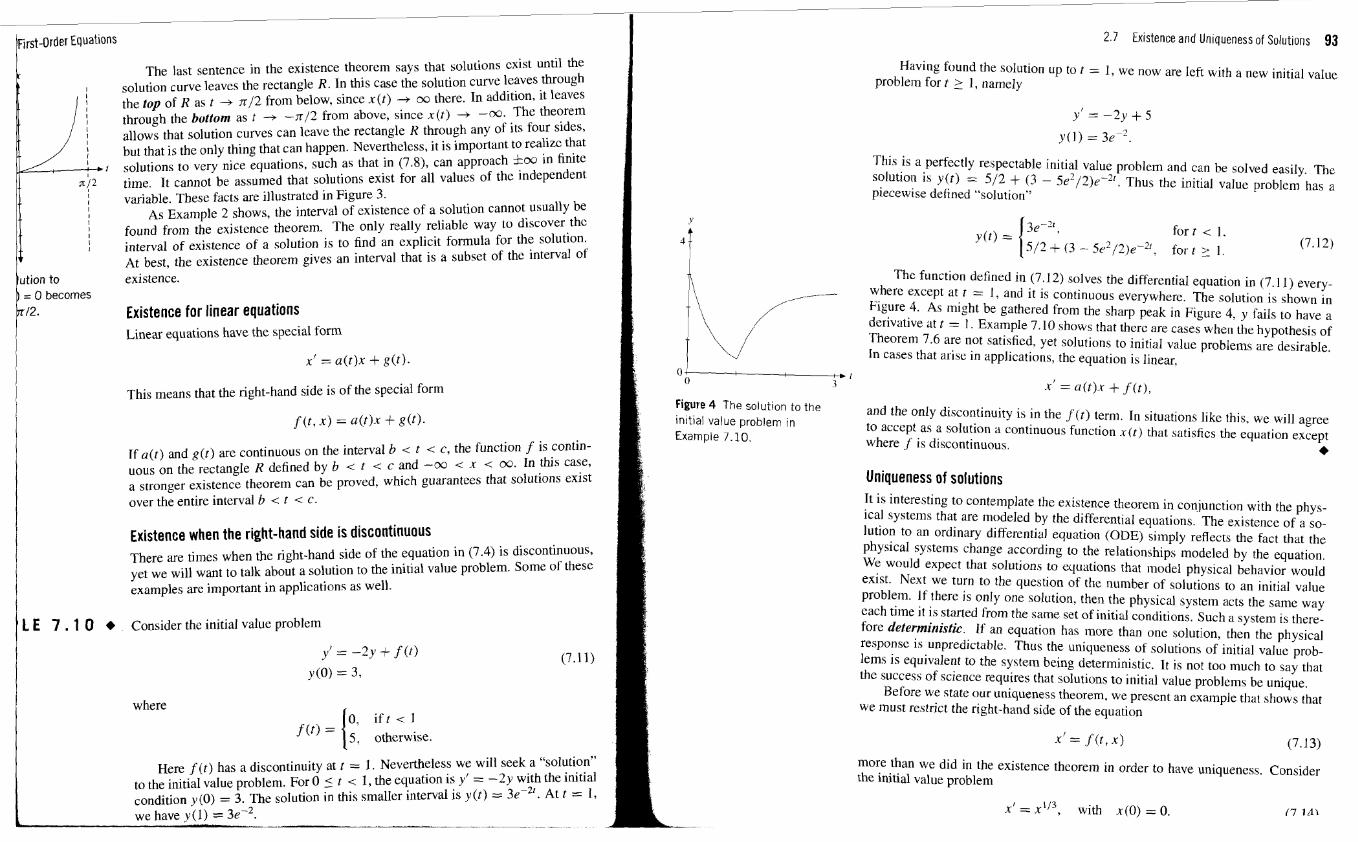
First-Order Equations
The last sentence in the existence theorem says that solutions exist until the 1 solution curve leaves the rectangle R. In this case the solution curve leaves through
\ the top of R as t + n / 2 from below, since x ( t ) + m there In addition, it Leaves I through the buttom as t + - n / 2 from above, since x ( r ) + -m. The theorem I allows that solution curves can leave the rectangle R through any of its four sides, I but that is the only thing that can happen. Nevertheless, it is important to realize that
t solutions to very nice equations, such as that in (7.8), can approach &CQ in finite
n(2 time. It cannot be assumed that solutions exist for all values of the independent i variable. These facts are illustrated in Figure 3. I As Example 2 shows, the interval of existence of a solution cannot usually be I
I found from the existence theorem. The only really reliable way to discover the I
I interval of existence of a solution is to find an explicit formula for the solution. v At best, the existence theorem gives an interval that is a subset of the interval of ution to existence.
) = 0 becomes n/2. Existence for linear equations
Linear equations have the special form
x' = a(t)x + g(t).
This means that the right-hand side is of the special form
If a ( t ) and g( t ) are continuous on the interval b c t < c, the function f is contin- uous on the rectangle R defined by b < t < c and -m < x < w. In this case, a stronger existence theorem can be proved, which guarantees that solutions exist over the entire interval b < t < c.
Existence when the right-hand side is discontinuous There are times when the right-hand side of the equation in (7.4) is discontinuous, yet we will want to talk about a solution to the initial value problem. Some of these examples are important in applications as well.
L E 7 . 1 0 + Consider the initial value problem
y' = -2y + f ( t )
y(0) = 3 ,
where
Here f ( t ) has a discontinuity at t = 1. Nevertheless we will seek a "solution" to the initial value problem. For 0 ( t < 1, the equation is y' = -2y with the initial condition y (0) = 3. The solution in this smaller interval is y( t ) = 3eC2*. At t = 1,
1 we have y ( I ) = 3e-2. . -
2.7 Existence and Uniqueness of Solutions 93
Having found the solution up to t = 1, we now are left with a new initial value problem for t > 1, namely
This is a perfectly respectable initial value problem and can be solved easily. The solution is g(t) = 512 + ( 3 - 5e2/2) r" . Thus the initial value problem has a piecewise defined "solution"
The function defined in (7.12) solves the differential equation in (7.1 1) every-
& where except at t = 1, and it is continuous everywhere. The solution is shown in Figure 4. As might be gathered from the sharp peak in Figure 4, y fails to have a derivative at t = I . Example 7 10 shows that there are cases when the hypothesis of Theorem 7.6 are not satisfied, yet solutions to initial value problems are desirable. In cases that arise in applications, the equation is linear,
0 1 3 x' = a(t)x + f ( t ) ,
Figure 4 The solution to the and the only discontinuity is in the J ( t ) term. In situations like this. we will agree initial value problem in
to accept as a solution a continuous function x ( t ) that satisfies the equation except Example 7.10. where f is discontinuous. 4
Uniqueness of solutions It is interesting to contemplate the existence theorem in con.junction with the phys- ical systems that are modeled by the differential equations. The existence of a so- lution to an ordinary differential equation (ODE) simply reflects the fact that the physical systems change according to the relationships modeled by the equation. We would expect that solutions to equations that model physical behavior would exist. Next we turn to the question of the number of solutions to an initial value problem. If there is only one solution, then the physical system acts the same way each time it is started from the same set of initial conditions. Such a system is there- fore deterministic. If an equation has inore than one solution, then the physical response is unpredictable. Thus the uniqueness of solutions of initial value prob- lems is equivalent to the system being deterministic. It is not too much to say that the success of science requires that solutions to initial value problems be unique.
Before we state our uniqueness theorem, we present an example that shows that we must restrict the right-hand side of the equation
more than we did in the existence theorem in order to have uniqueness. Consider the initial value problem
= x 1 / 3 , with x(0) = 0.
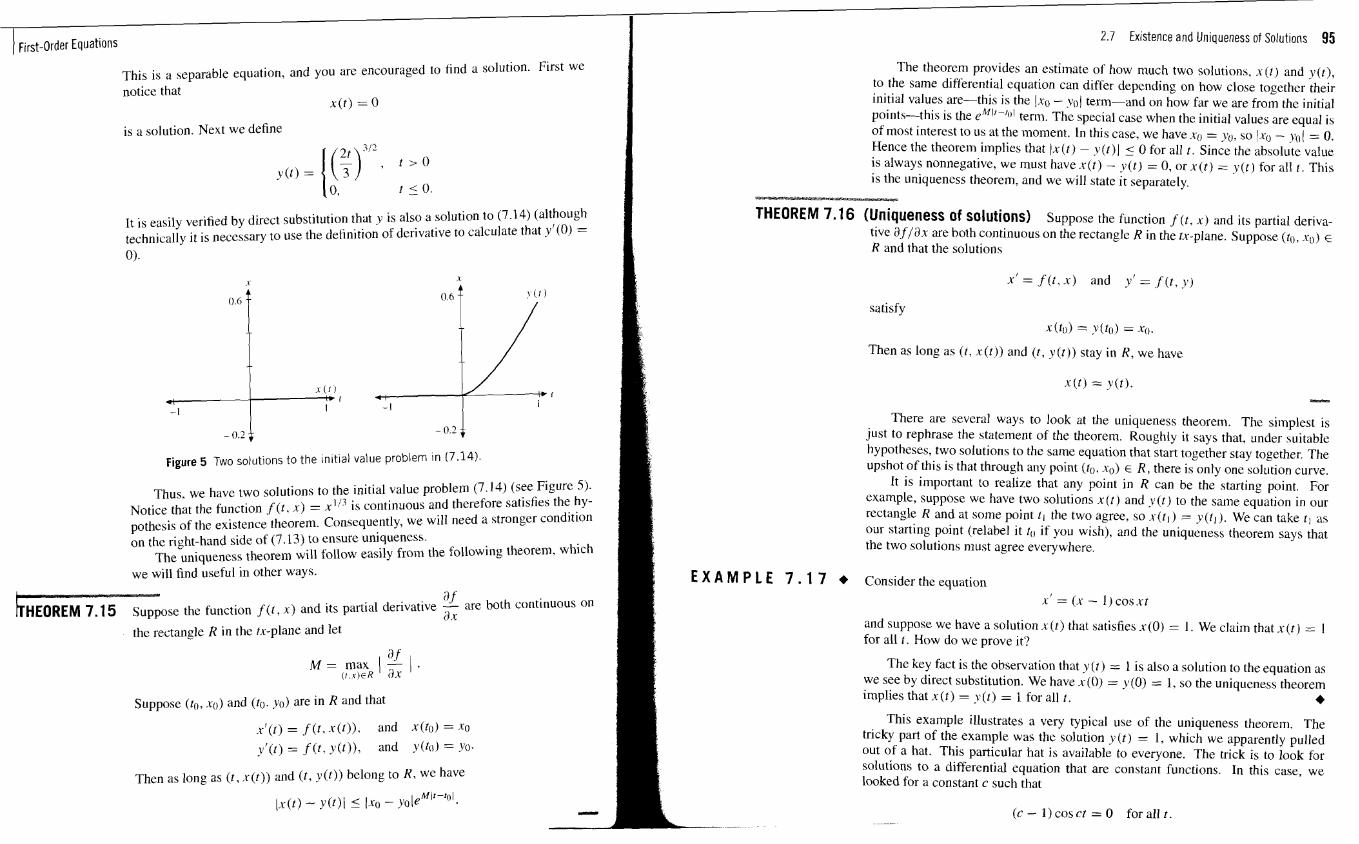
First-Order Equations
This is a separable equation, and you are encouraged to find a solution. First we notice that
x(t) = 0
is a solution. Next we define
It is easily verified by direct substitution that y is also a solution to (7.14) (although technically it is necessary to use the definition of derivative to calculate that y'(0) = 0).
Figure 5 Two solutions to the initial value problem in (7.14)
Thus. we have two solutions to the initial value problem (7.14) (see Figure 5) . Notice that the function f (t. x) = x'/ ' is continuous and therefore satisfies the hy- pothesis of the existence theorem. Consequently, we will need a stronpr condition on the right-hand side of (7.13) to ensure uniqueness.
The uniqueness theorem will follow easily from the following theorem. which we will find useful in other ways.
3 f ose the function f (t, x) and its partial derivative - a ,l- are both continuous on
the rectangle R in the t-r-plane and let
B f M = max 1 - 1 .
( I . x ) E R
Suppose (to, so) and (to, yo) are in R and that
xl(t) = f (t, x (t)), and x (to) = xo
y'(t) = f (t, y(t)), and y(to) = yo.
Then as long as (t, x(t)) and (t, y (t)) belong to R, we have
2.7 Existence and Uniqueness of Solutions 95
The theorem provides an estimate of how much two solutions, x(t) and y(t), to the same differential equation can differ depending on how close together their initial values are-this is the 1x0 - yo1 term-and on how far we are from the initial points-this is the eMl'-'~l term. The special case when the initial values are equal is of most interest to us at the moment. In this case, we have xo = yo, SO JxO - yo/ = 0. Hence the theorem implies that Ix (t) - y (t) 1 ( 0 for all t . Since the absolute value is always nonnegative, we must have .u(t) - y (t) = 0, or x(t) = y ( t ) for all t. This is the uniqueness theorern, and we will state it separately.
T H E O R E M 7.16 (Uniqueness of solutions) Suppose the function f (t. x) and its partial deriva- tive a f /ax are both continuous on the rectangle R in the tx-plane. Suppose (to, xu) E
R and that the solutions
x' = f (t, x ) and y' = f ( t , p)
satisfy
Then as long as ( t , x(t)) and (t, y(t)) stay in R, we have
There are several ways to look at the uniqueness theorem. The simplest is just to rephrase the statement of the theorem. Roughly it says that, under suitable hypotheses, two solutions to the same equation that start together stay together. The upshot of this is that through any point (to, xo) E R , there is only one solution curve.
It is important to realize that any point in R can be the starting point. For example, suppose we have two solutions x(t) and y(t) to the same equation in our rectangle R and at some point tj the two agree, so x( t l ) = y (tl). We can take ti as our starting point (relabel it to if you wish), and the uniqueness theorern says that the two solutions must agree everywhere.
E X A M P E 7 . 1 7 + Consider the equation
and suppose we have a solution x( t ) that satisfies x(0) = 1. We claim that x(t) = 1 for all t. How do we prove it?
The key fact is the observation that y(t) = 1 is also a solution to the equation as we see by direct substitution. We have x(0) = y(0) = 1, so the uniqueness theorem implies that x(t) = y ( t ) = 1 for all t. +
This example illustrates a very typical use of the uniqueness theorem. The tricky part of the example was the solution y (t) = 1, which we apparently pulled out of a hat. This particular hat is available to everyone. The trick is to look for solutions to a differential equation that are constant functions. In this case, we looked for a constant c such that
-. A -
(c - 1) cos ct = 0 for all t .
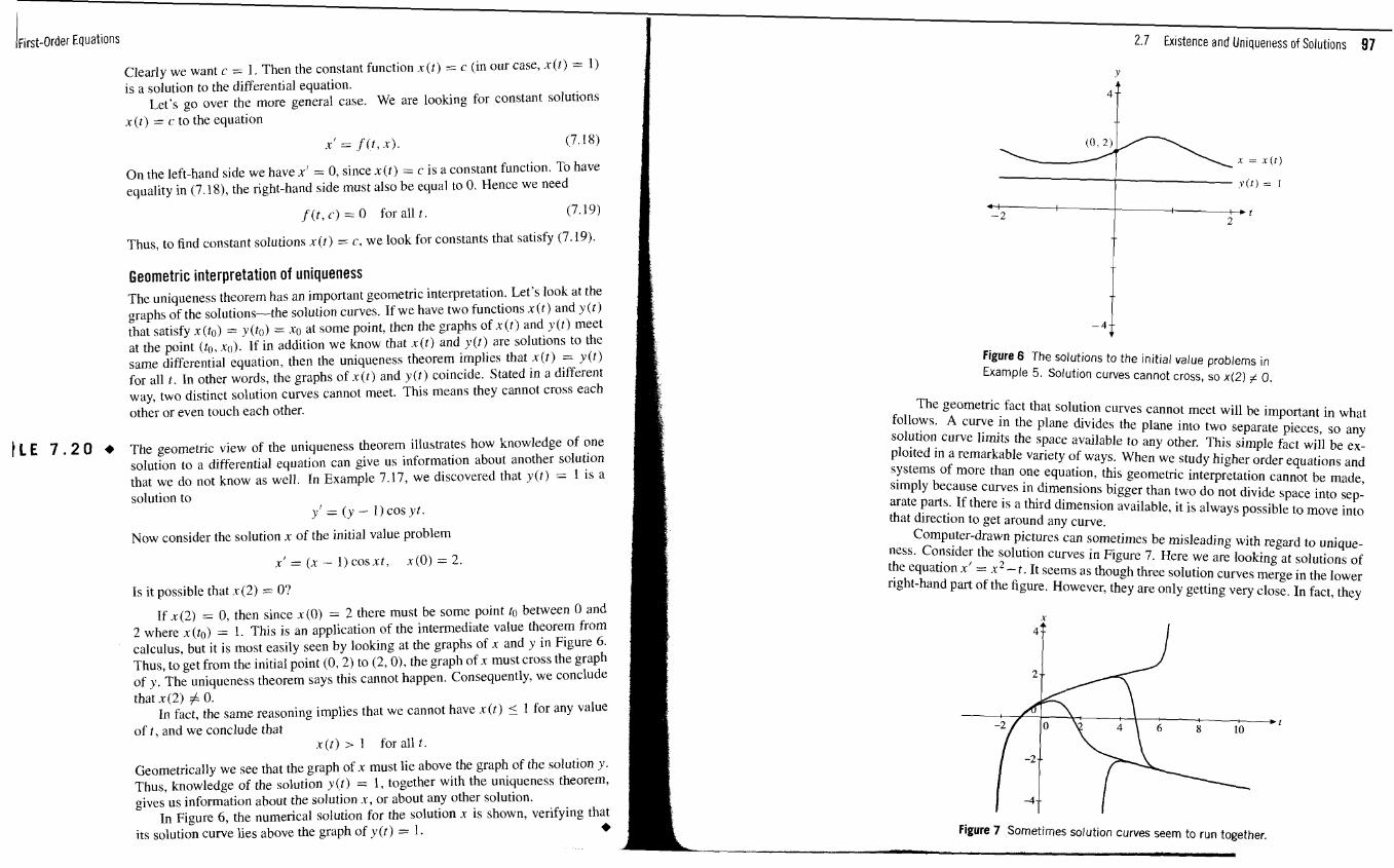
I 2.7 Existence and Uniquerless of Solutions 97 first-Order Equations
Clearly we want c = 1. Then the constant function x ( t ) = c (in our case, x ( t ) = 1) is a solution to the differential equation.
Let's go over the more general case. We are looking for constant solutions x ( t ) = c to the equation 1 On the left-hand side we have x' = 0, since x ( t ) = c is a constant function. To have equality in (7.18). the right-hand side must also be equal to 0. Hence we need
,f ( t , r ) = 0 for all t . (7.19)
Thus, to find constant solutions x ( t ) = c, we look for constants that satisfy (7.19).
Geometric interpretation of uniqueness The uniqueness theorem has an important geometric interpretation. Let's look at the graphs of the solutions-the solution curves. If we have two functions x ( t ) and y ( r ) that satisfy x (to) = y(to) = .KO at some point, then the graphs of x ( t ) and y ( t ) meet at the point (to, x u ) If in addition we know that x ( t ) and y( t ) are solutions to the same differential equation, then the uniqueness theorem implies that x ( t ) = y( t ) for all t . In other words, the graphs of x ( t ) and y ( t ) coincide. Stated in a different way, two distinct solution curves cannot meet. This means they cannot cross each other or even touch each other.
L E 7 . 2 0 The geometric view of the uniqueness theorem illustrates how knowledge of one solution to a differential equation can give us information about another solution that we do not know as well. In Example 7.17, we discovered that y(t) = 1 is a solution to
= ( y - 1) cos y t .
Now consider the solution x of the initial value problem
Is it possible that s ( 2 ) = O?
If x(2) = 0, then since x(0) = 2 there must be some point to between 0 and 2 where x(to) = 1. This is an application of the intermediate value theorem from calculus, but it is most easily seen by looking at the graphs of x and y in Figure 6. Thus, to get from the initial point (0 ,2 ) to (2.0). the graph of r must cross the graph of v. The uniqueness theorem says this cannot happen. Consequently, we conclude that x(2) # 0,
In fact, the same reasoning implies that we cannot have n ( t ) <_ 1 for any value of t , and we conclude that
x ( t ) > 1 foral l t .
Geometrically we see that the graph of x must lie above the graph of the solution y . Thus, knowledge of the solution y(t) = 1, together with the uniqueness theorem, gives us information about the solution .r, or about any other solution.
In Figure 6, the numerical solution for the solution x is shown, verifying that its solution curve lies above the graph of y ( t ) = 1 .
Figure 6 The solutions to the initial value problems in Example 5. Solution curves cannot cross, so x(2) # 0.
The geometric fact that solution curves cannot meet will be important in what follows. A curve in the plane divides the plane into two separate pieces, so any solution curve limits the space available to any other. This simple fact will be ex- ploited in a remarkable variety of ways. When we study higher order equations and systems of more than one equation, this geometric interpretation cannot be made, simply because curves in dimensions bigger than two do not divide space into sep- arate pa.rts. If there is a third dimension available, it is always possible to move into that direction to get around any curve,
Computer-drawn pictures can sometimes be misleading with regard to unique- ness. Consider the solution curves in Figure 7. Here we are looking at solutions of the equation x' = x2 - t . It seems as though three solution curves merge in the lower right-hand part of the figure. However, they are only getting very close. In fact, they
Figure 7 Sometimes solution curves seem to run together.
I
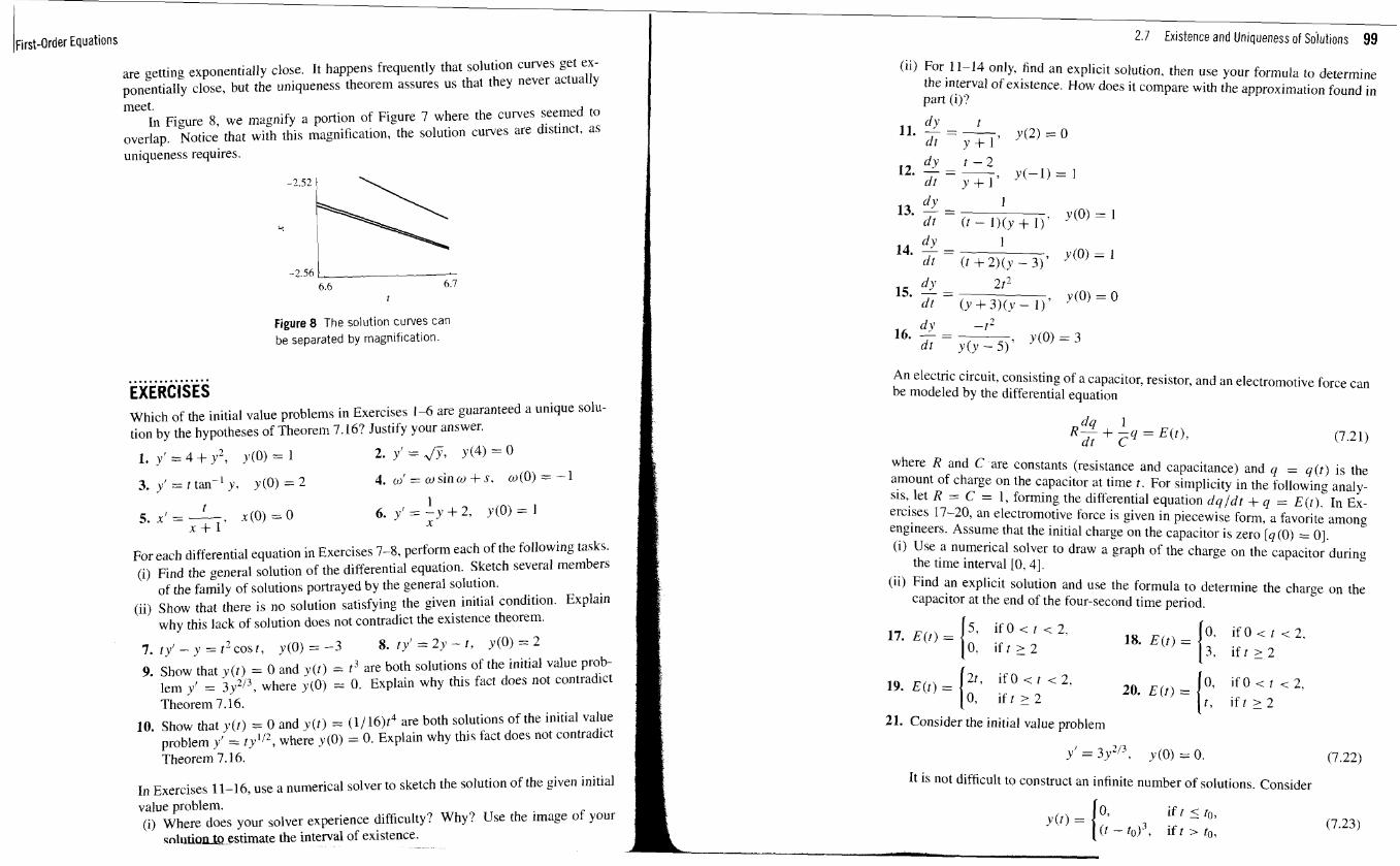
first-Order Equations
are getting exponentially close. It happens frequently that solution curves get ex- ponentially close, but the uniqueness theorem assures us that they never actually meet.
In Figure 8, we magnify a portion of Figure 7 where the curves seemed to overlap. Notice that with this magnification, the solution curves are distinct. as uniqueness requires.
Figure 8 The solution curves can be separated by magnification.
................ EXERCISES Which of the initial value problems in Exercises 1-6 are guaranteed a unique solu- tion by the hypotheses of Theorem 7.16? Justify your answer.
1. y' = 4 + Y2, y(0) = 1 2. y ' = a , y ( 4 ) = 0
For each differential equation in Exercises 7-8, perform each of the following tasks. (i) Find the general solution of the differential equation. Sketch several members
of the family of solutions portrayed by the general solution. (ii) Show that there is no solution satisfying the given initial condition. Explain
why this lack of solution does not contradict the existence theorem.
7. ty! - y = t2 cost, y(0) = -3 8. ty' = 2y - t , y(0) = 2
9. Show t h a y (t) = 0 and y (1) = t b r e both solutions of the initial value prob- lem y' = 3y2I3, where y(0) = 0. Explain why this fact does not contradict Theorem 7.16.
10. Show that y(t) = 0 and y(t) = ( I / 16)t4 are both solutions of the initial value problem y' = ty1I2, where y(0) = 0. Explain why this fact does not contradict Theorem 7.16.
In Exercises 11-16, use a numerical solver to sketch the solution of the given initial value problem. (i) Where does your solver experience difficulty? Why? Use the image of your
sn1ution-Q estimate the interval of existence.
2.7 Existence and Uniqueness of sdutions 99
(ii) For 11-14 only, find an explicit solution. then use your formula to deterlnine the interval of existence. How does it compare with the approximation found in part (i)'?
An electric circuit, consisting of a capacitor, resistor, and an electromotive force can be modeled by the differential equation
where R and C are constants (resistance and capacitance) and q = q(r) is the amount of charge on the capacitor at time t For simplicity in the following analy- sis, let R = C = I, forming the differential equation dq/dr + q = E(t). In Ex- ercises 17-20, an electromotive force is given in piecewise form, a favorite among engineers. Assume that the initial charge on the capacitor is zero [q(O) = 01. (i) Use a numerical solver to draw a graph of the charge on the capacitor during
the time interval [0,4]. (ii) Find an explicit solution and use the formula to determine the charge on the
capacitor at the end of the four-second time period.
, 21. Consider the initial value problem
y' = 3y2I3, y(0) = 0. (7.22) It is not difficult to construct an infinite number of solutions. Consider
i ~ i rs t -o rder Equations
where to is any positive number. It is easy to calculate the derivative of y(t). when t # to,
but the derivative at to remains uncertain.
(a) Evaluate both
showing that
i f t 5 to, y'(r) = iff > to .
(b) Finally, show that y (t) is a solution of (7.22). Why doesn't this example contradict Theorem 7.16?
22. Consider again the "solution" of equation (7.1 1) in Example 3,
I 3e-2', for t < 1, y(t) = 512 + (3 - 5e2/2)eP2' for t >_ 1.
(a) Follow the lead in Exercise 21 to calculate the derivative of y (t).
(b) In the sense of Definition 1 from Section 2.1, is y(t) a solution of (7.11)? Why or why not?
(c) Show that y (t) satisfies equation (7.11) for all t except t = 1.
23. Show that
0, for t < 0,
is a solution of the initial value problem ty' = 4y, where y (0) = 0, in the sense of Definition 1 from Section 2.1. Find a second solution and explain why this lack of uniqueness does not contradict Theorem 7.16.
24. Uniqueness is not just an abstraction designed to please theoretical mathemati- cians. For example, consider a cylindrical drum filled with water. A circular drain is opened at the bottom of the drum and the water is allowed to pour out. Imagine that you come upon the scene and witness an empty drum. YOU have no idea how long the drum has been empty. Is it possible for you to determine when the drum was full? (a) Using physical intuition only, sketch several possible graphs of the height
of the water in the drum versus time. Be sure to mark the time that you appeared on the scene on your graph.
2.7 Existence and Uniqueness of Solutions 101
(b) It is reasonable to expect that the speed at which the water leaves through the drain depends upon the height of the water in the drum. Indeed, Tori- celli's law predicts that this speed is related to the height by the formula v2 = 2gh, where g is the acceleration due to gravity near the surface of the earth. Let A and a represent the area of a cross section of the drum and drain, respectively. Argue that A Ah = av At, and in the limit, A dh ld t = av. Show that dh ld t = - ( a / A ) a .
(c) By introducing the dimensionless variables o = a h and s = fit and then choosing parameters
1 a = - and /3 = (z) /$,
11 0
where ho represents the height of a full tank, show that the equation dh ld t = -(a/A)&$ becomes dwlds = - fi. Note that when w = 0. the tank is empty, and when w = 1, the tank is full.
(d) You come along at time s = so and note that the tank is empty. Show that the initial value problem, dwlds = -fi, where ul(so) = 0, has an infi- nite number of solutions. Why doesn't this fact contradict the uniqueness theorem? Hint: The equation is separable and the graphs you drew in part (a) should provide the necessary hint on how to proceed.
25. Is it possible to find a function f ( t , x) that is continuous and has continuous partial derivatives such that the functions x 1 (t) = t and x2 (t) = sin t are both solutions to x' = f (t, x) near t = O?
26. Is it possible to find a function f (t, x ) that is continuous and has continuous partial derivatives such that the functions XI (t) = cos t and x2(t) = 1 - sin t are both solutions to x' = f (t, x) near t = n/2?
27. Suppose that x is a solution to the initial value problem
x ' = x c o s 2 t and x(O)= 1.
Show that x(t) > 0 for all t for which x is defined.
28. Suppose that y is a solution to the initial value problem
yf = ( y - 3)ecos(t~) and y ( l ) = l
Show that y (t) < 3 for all t for which y is defined.
29. Suppose that y is a solution to the initial value problem
2 yr = (y - l)etY and y ( l ) = 0.
Show that -1 < y(t) < 1 for all t for which y is defined.
30. Suppose that x is a solution to the initial value problem
x 3 - x x =-
1 + t2x2 and x (0 )=1 /2 .
Show that 0 < x ( t ) < 1 for all t for which x is defined.
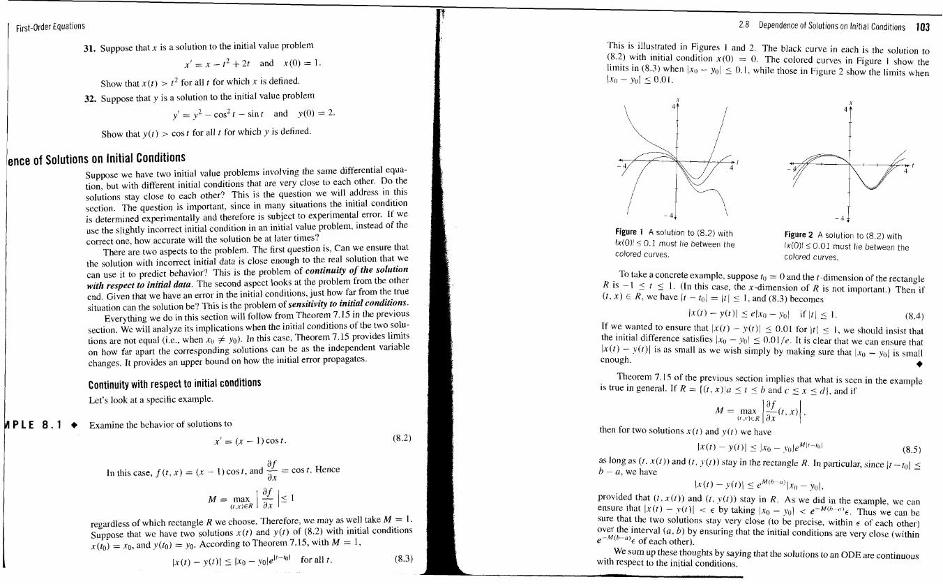
I First-Order Equations
31. Suppose that x is a solution to the initial value problem 2 . r l = x - r + 2 t and x ( 0 ) = 1 .
Show that x( t) > t2 for all r for which x is defined.
32. Suppose that y is a solution to the initial value problem 2 y ' = y 2 - c o s t - s i n t and y ( 0 ) = 2 .
1 Show that y(t) > cost for all t for which y is defined.
ence of Solutions on Initial Conditions Suppose we have two initial value problems involving the same differential equa- tion, but with different initial conditions that are very close to each other. Do the solutions stay close to each other? This is the question we will address in this section. The question is important, since in many situations the initial condition is determined experimentally and therefore is subject to experimental error. If we use the slightly incorrect initial condition in an initial value problem. instead of the correct one, how accurate will the solution be at later times?
There are two aspects to the problem. The first question is, Can we ensure that the solution with incorrect initial data is close enough to the real solution that we can use it to predict behavior? This is the problem of continuity of the solution with respect to initial data. The second aspect looks at the problem from the other end. Given that we have an error in the initial conditions, just how far from the true situation can the solution be? This is the problem of sensitivity to initial conditions.
Everything we do in this section will follow from Theorem 7.15 in the previous section. We will analyze its implications when the initial conditions of the two solu- tions are not equal (i.e., when xu # yo). In this case, Theorem 7.15 provides limits on how far apart the corresponding solutions can be as the independent variable changes. It provides an upper bound on how the initial error propagates.
Continuity with respect to initial conditions Let's look at a specific example.
P L E 8 . 1 + Examine the behavior of solutions to
x' = (x - 1) cos I. (8.2)
a f In this case, f ( t , x) = (x - 1) cost, and - = cost. Hence ax
I af M = mar 1-/51
( t . x ) ~ R a , ~ regardless of which rectangle R we choose. Therefore, we may as well take M = 1. Suppose that we have two solutions x(t) and y(t) of (8.2) with initial conditions x(to) = xo, and y(to) = yo. According to Theorem 7.15, with M = 1,
( ~ ( t ) - y(t)l 5 1x0 - vo(e't-tO' for all t.
2.8 Dependence of Solutions on Initial Conditions 103
This is illustrated in Figures I and 2. The black curve in each is the solution to ( 8 2 ) with initial condition x(0) = 0. The colored curves in Figure I show the limits in (8.3) when lxo - yo1 i 0. I, while those in Figure 2 show the limits when 1x0 - yo1 ( 0.01.
Figure 1 A solution to (8.2) with Figure 2 A solution to (8.2) with Ix(0)I 1 0 . 1 must lie between the Ix(O)I 1 0.01 must lie between the colored curves. colored curves.
To take a concrete example, suppose to = 0 and the t-dimension of the rectangle R is -1 5 t 5 I. (In this case, the x-dimension of R is not important.) Then if (t. x ) E R , we have It - tol = It1 i I . and (8.3) becomes
(x(t) - y(t)l i el.xo - yo1 if It1 5 1 . (8.4) If we wanted to ensure that Ix(t) - y(t)l i 0.01 for It ( 5 1 , we should insist that the initial difference satisfies (xu - yoJ 5 0.01/e. It is clear that we can ensure that Ix(t) - y(t)I is as small as we wish simply by making sure that Ixo - y[)l is small enough. +
Theorem 7 15 of the previous section implies that what is seen in the example is true in general. If R = {(t, x)lu i t 5 b and c 5 x 5 ( I } , and if
M = max -(r.xj , ( r ) ) E K l a f ax I
then for two solutions x(t ) and y (t) we have
Ix(t) - y(t)J 5 Ixo - voleMtpt(lI (8.5) as long as (r. x( t)) and (t, ~ ( r ) ) stay in the rectangle R. In particular, since It -to/ 5 b - u, we have
(x(t) - p(t)l i e"(hp") 1x0 - yol, E provided that ( t , x(t)) and (t. ~ ( r ) ) stay in R. As we did in the example. we can
ensure that Ix(t) - !(r)l < 6 by taking 1x0 - yo] < e-M(hp"'e. Thus we can be sure that the two solutions stay very close (to be precise, within 6 of each other) over the interval (a, b) by ensuring that the initial conditions are very close (within e - ~ ( b - ~ ) c of each other).
We sum up these thoughts by saying that the solutions to an ODE are continuous with respect to the initial conditions.
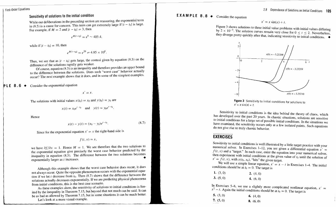
1 Arst-Order Equations
Sensitivity of solutions to the initial condition While our deliberations in the preceding section are reassuring, the exponential term in (8.5) is a cause for concern. This term can get extremely large if It - to1 is large. For example, if M = 2 and It - to1 = 3, then
while if It - to1 = 10, then
Thus, we see that as It - tot gets large, the control given by equation (8.5) on the difference of the solutions rapidly gets weaker.
Of course, equation (8.5) is an inequality and therefore provides an upper bound to the difference between the solutions. Does such "worst case" behavior actually occur'? The next example shows that it does, and in some of the simplest examples.
P L E 8 . 6 + Consider the exponential equation I x = x.
The solutions with initial values x(to) = xo and y(to) = yo are
~ ( t ) = x ~ ~ ~ ~ - ~ O and y(t) = yoe'-'O.
Hence
x(t) - y(t) = (xo - yo)e'-'O
Since for the exponential equation x' = x the right-hand side is
we have af / a . = 1. Hence M = 1. We see therefore that the two solutions to the exponential equation give precisely the worst case behavior predicted by the inequality in equation (8.5). The difference between the two solutions becomes exponentially larger as t increases.
+
Although this example shows that the worst case behavior does occur, it does not always occur. Quite the opposite phenomenon occurs with the exponential equa- tion if we let t decrease from to. Then (8.7) shows that the Qfference between the solutions actually decreases exponentially. If we are predicting physical phenomena from initial conditions, this is the best case scenario.
As these examples show, the sensitivity of solutions to initial conditions is lim- ited by the inequality in Theorem 7.15, but beyond that not much can be said. It can be as bad as allowed by Theorem 7.15, but in some situations it can be much better.
Let's look at a more visual example.
2.8 Dependence of Solutions on Initial Conditions 105
E X A M P L E 8 . 8 Consider the equation
x' = x sin(x) + t . Figure 3 shows solutions to three initial value problems with initial values differing by 2 x l0-I. The solution curves remain very close for 0 5 t 5 2. Nevertheless, they diverge pretty quickly after that, indicating sensitivity to initial conditions. 4
Figure 3 Sensitivity to initial conditions for solutions to x' = x sin(x) + t.
Sensitivity to initial conditions is the idea behind the theory of chaos, which has developed over the past 20 years. In chaotic situations, solutions are sensitive to initial conditions for a large set of possible initial conditions. In the situations we have examined, the sensitivity occurs only at a few isolated points. Such equations do not give rise to truly chaotic behavior.
................ EXERCISES Sensitivity to initial conditions is well illustrated by a little target practice with your numerical solver. In Exercises 1-12, you are given a differential equation x' = f (t, x) and a "target." In each case, enter the equation into your numerical solver, then experiment with initial conditions at the given value of to until the solution of x' = f ( t , x), with x(t0, xo), "hits" the given tareet. - " We will use a simple linear equation, x' = x - t in Exercises 1 4 . The initial conditions should be at to = 0. The target is
In Exercises 5-8, we use a slightly more complicated nonlinear equation, x f = x2 - t. Again the initial conditions should be at to = 0. The target is
5. (390) 6. (4,O)
7. (590) 8. (6.01
1 First-Order Equations
For Exercises 9-12, we use the equation in Example 8.8, x' = ,x sinx + t. Again the initial conditions should be at to = 0. The target is
9. (3,O) 10. (4,O)
11. (5,O) 12. (6,O)
13. This exercise addresses a very cornmon instance of a motion that is sensitive to initial conditions. Flip a coin with your thumb and forefinger, and let the coin land on a pillow. The motion of the coin is governed by a system of ordinary differential equations. It is not immediately important what that system is. It is only important to realize that the motion is governed entirely by the initial con- ditions (i.e., the upward velocity of the coin and the rotational energy impded to it when it is flipped). If the motion were not sensitive to initial conditions, it would be possible to learn how to Rip ten heads in a row. Try to learn how to do this, and report the longest chain of heads you are able to achieve.
The flipping of a coin is often considered to have a random outcome. In fact the result is determined by the initial conditions. It is the sensitivity of the result to the initial conditions that gives the appearance of randomness. - -
Let's plot the error bounds shown in Figure 1. First, solve x' = (x - 1) cos t . x(0) = 0, and plot the solution over the interval [-4.41. Next, as we saw in Example 8.1. if y(t) is a second solution with 1,x (0) - y(O)I 5 0.1. then the inequality (8.3) becomes lx(t) - y(t)l 5 0.lelC'. Solve this inequality for x(t). placing your final answer in the form eL(t) 5 x (t) 5 e~ (I); then add the graphs of eL(t) and eH(t) to your plot. How can you use Theorem 7.15 to show that no solution starting with initial condition lx(0) - y(O)( 5 0.1 has any chance ..- - - of rising as far as indicated by eH (t)'!
15. Draw the enor bounds shown in Figure 2. See Exercise 14 for assistance.
16. Consider the equation x' = (x - 1) cos t . (a) Let x(t) and y (1) be two solutions. What is the upper bound on the separa-
tion Ix (t) - y(t)l predicted by Theorem 7.15?
(b) Find the solution x(t) with initial value x(0) = 0, and the solution y(t) with initial value y(0) = 1/10. Does the separation x(t) - y(t) satisfy the inequality found in part (a)'?
(c) Are there any values of t where the separation achieves the maximum pre- dicted?
17. Consider x' + 2x = sin t.
(a) Let x(t) and y(t) be two solutions. What is the upper bound on the separa- tion Ix(t) - y(t)( predicted by Theorem 7.15?
(b) Find the solution x (t ) with initial value .x (0) = - 115, and the solution y (t) with initial value y(0) = -3110. Does the separation x(t) - y(t) satisfy the inequality found in part (a)?
(c) Are there any values of t where the separation achieves the maximum pre- dicted?
2.9 Autonomous Equations and Stability 107
18. Let x, (t) and xi@) be solutions of x' = x2 - r having initial conditions x1 (0) = 0 and ~ ( 0 ) = 314. Use Theorem 7.15 to determine an upper bound for 1x1 ( t ) - xl(t)l, as long as the solutions x l ( t ) and x ? ( t ) remain inside the rect- angle defined by R = ((t, x ) : - 1 5 t 5 1, -2 < x 2). Use your numerical - solver to draw the solutions xl (1) and xz(t), restricted to the rectangular region R. Estimate m a x ~ 1x1 (1) - x2 (1) 1 and compare with the estimated upper bound.
2.9 Autonomous Equations and Stability A first-order autonomous equation is an equation of the special form
x' = f (x). (9.1)
Notice that the independent variable, which we have usually been denoting by t, does not appear explicitly on the right-hand side of equation (9.1). This is the defin- ing feature of an autonomous e~uation.
In Section 2.3, we derived the differential equation for the velocity of a weight dropping near the surface of the earth. It is
where g is the acceleration due to gravity, m is the mass of the body, and k is a proportionality constant. This is an autonomous equation. Other examples are
XI = sin(x), y' = y2 + 1, and zt = e z .
The equations
are not autonomous. The presence of the independent variable on the right-hand side of each equation implies that the equation is not autonomous.
Autonomous equations occur very frequently in applications. A differential equation model of any physical system that is evolving without external forces will be autonomous. It is usually the external forces that give rise to terms that depend explicitly on time.
The direction field and solutions Since the function f (t, x ) on the right-hand side of (9. I) does not depend on t, the
I
r slopes of the direction lines have the same feature. This is illustrated by the direction field for equation (9.2) shown in Figure I. The slopes do not change as we move 1 from right to left in this figure.
Because of this fact, we would expect the same behavior for the solution curves. We would expect that one solution curve translated to the Ieft or right would be another solution curve. We can see this analytically.
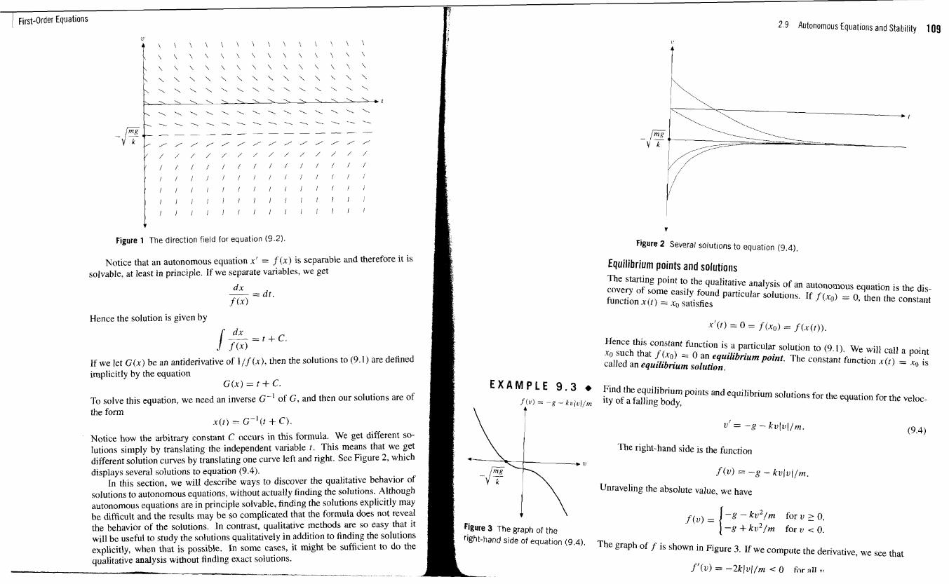
1 First-Order Equations
Figure 1 The direction field for equation (9.2).
Notice that an autonomous equation x' = f (x) is separable and therefore it is solvable, at least in principle. If we separate variables, we get
dx - = d t . f (.u)
Hence the solution is given by
If we let G ( x ) be an antiderivative of 1 / f ( x ) , then the solutions to (9.1 ) are defined implicitly by the equation
G(.u) = t + C.
To solve this equation, we need an inverse G-' of G, and then our solutions are of the form
x ( t ) = ~ - ' ( t + C).
Notice how the arbitrary constant C occurs in this formula. We get different so- lutions simply by translating the independent variable t . This means that we get different solution curves by translating one curve left and right. See Figure 2 , which displays several solutions to equation (9.4).
In this section, we will describe ways to discover the qualitative behavior of solutions to autonomous equations, without actually finding the solutions. Although autonomous equations are in principle solvable, finding the solutions explicitly may be difficult and the results may be so complicated that the formula does not reveal the behavior of the solutions. In contrast, qualitative methods are so easy that it will be useful to study the solutions qualitatively in addition to finding the solutions explicitly, when that is possible. In some cases, it might be sufficient to do the qualitative analysis without finding exact solutions.
rl/ln
. U
I).
2.9 Autonomous Equations and Stability 109
?
Figure 2 Several solutions to equation (9.4).
Equilibrium points and solutions The starting point to the qualitative analysis of an autonomous equation is the dis- covery of some easily found particular solutions. If f ( x g ) = 0, then the constant function x ( t ) = xo satisfies
Hence this constant function is a particular solution to (9.1). We will call a point xo such that f (xo) = 0 an equilibrium point. The constant function x ( t ) = ro is called an equilibrium solution.
Find the equilibrium points and equilibrium solutions for the equation for the veloc- ity of a falling body,
/ v = - g - k v lv l lm.
The right-hand side is the function
f ( v ) = -g - k t l ( v ( / m .
Unraveling the absolute value, we have
-g - k v 2 / m for v L 0, f (u ) = -6 + k v 2 / m for v i 0.
The graph of f is shown in Figure 3. If we compute the derivative. we see that
f ' ( v ) = -2klvl/m < 0 for 211 9 1
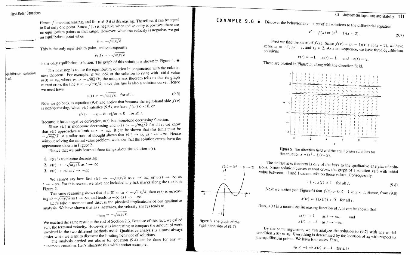
First-Order Equations
Hence f is nonincreasing, and for u # 0 it is decreasing. Therefore. it can be equal to 0 at only one point. Since j ( v ) is negative when the velocjty is positive. there are no equilibrium points in that range. However. when the velocity is neglive. we get an equilibrium point when
F - H 1 v = -Ja. This is the only equilibrium point, and consequently
r--- t ) , ( t ) = -v m g / k
i s the only equilibrium solution. The graph of this solution is shown in Figure 4. 4 .- - -
The next step is to use the equilibrium solution in conjunction with the unique- !quilibrlum so'ution ness theorem. For example, if we look at the solution to (9.4) with initial value ).4). "(0) = uo, where un > -,/*. the unique~~ess theorem tells us that its graph
cannot cross the line u = ,/m. since this line is also a solution curve. Hence we must have
,(t) > - JG for all t .
Now we go back to equation (9.4) and notice that because the right-hand side f ( a ) is nondecrcasing, when v ( t ) satisties (9.5). we have f ( u ( t ) ) < 0, or
vl(r) = -g - kulvl/m < 0 for all t .
Because it has a negative derivative. u( t ) is a monulone decreasing function. Since u(r) is monotone decreasing and u( t ) > - Js for all t . we know
that a(t) approaches a limit as t -+ m It can be shown that this limit must be - A similar tram of thought shows that v ( t ) 4 ca as t -r -03. Hence without solving the initial value problem, we know that the solution curvea have the appearance shown in Figure 2.
Notice that we only learned threc things about the solution I ) ( [ ) :
1. v ( t ) is monotone decreasing
2. v ( t ) -+ -,I* as t -+ oo 3. tl(t) -+ cc as t -+ -cc
We cannot say how fast r ( t ) -+ -Ja as t 4 w, or L J ( ~ ) 4 ~o as t -+ -oo. For this reason, we have not included any tick marks along the r axis in Figure 2.
The same reasoning shows that ~f v(0) = ua < - d s , then u ( t ) is increas- ing to -e as f + w , and tends to -oc as t -t -CQ.
Let's take a moment and discuss the physical implications of our qualitative analysis. We hake shown that as t Increases, the velocity always tends to
We reached the same result at the end of Section 2.3. Because of this fact, we called a,,,, the terminal velocity. However, it is interesting to compare the amount of work involved in the two different methods used. Qualitative analysis is almost always easier when we want to discover the limiting behavior of solutions.
The analysis camed out above for equation (9.4) can be done for any au- 4 n - - m n ~ ~ ~ eauation. Let's illustrate this with another example.
2.9 Autonomous Equations and Stabilitv 11 1 E X A M P L E 9 . 6 + Discover the behavior as t -+ oc of all solutions to the differential equation
First we find the zeros of f ( x ) . Since f ( x ) = ( x - 1)(x + l ) ( x - 2). we have zeros X I = -1, xi = I . and x? = 2. As a consequence, we have three equilibrium solutions
~ ( t ) = -1, x ( t ) = 1 , and x ( t ) = 2. These are plotted in Figure 5, along with the direction field.
Figure 5 The direction field and the equilibrium solutions for the equation x ' = ( x2 - 1 ) ( x - 2 ) .
The uniqueness thcorem is one of the keys to the qualitative analysis of solu- f ( x ) = (x? - I ) ( X - 2 tions. Since solution curves cannot cross. the graph of a solution x ( t ) with initial
value between - 1 and 1 cannot take on those values. Consequently,
Thus. x ( t ) is a nlonotone increasing function of t . It can be shown that 1-11 x(t) --t 1 as t --t oo, and Figure 6 The graph of the ( t - as t - - t -oc . right-hand side of (9.7).
By the samc argument, we can analyze the solution to (9.7) with any initial condition x(0) = q. Everything is determined by the location of xo with respect to the equilibrium points. We have four cases. First,
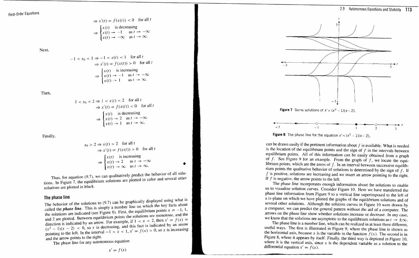
First-Order Equations
Next,
+ xf(t) = f (x(f)) < 0 for all t
x (t) is decreasing x ( t ) + - 1 a s t - + - m x(t) -. -CC, as t w.
- l < x o < l + - I < x ( t ) r l forallt 3 x' (t) = f (x(t)) > 0 for all t
x (t) is increasing x(t) -t -1 as t 4 -oo x ( t ) - + l a s t 4 X .
Then,
1 < x o < 2 j 1 < x ( t ) < 2 foral l t
j ~ ' ( t ) = f (x(t)) < 0 for all t
x (t ) is decreasing x ( t ) - 2 a s t - -02
x ) a s t - m .
Finally,
xo > 2 j x ( t ) > 2 forallt j x r ( t ) = f ( s ( t ) ) > 0 foral l t
x (t) is increasing x ( t ) + 2 a s t + - o o x(t) 4 CC, as t + oo. +
Thus. for equation (9.7), we can qualitatively predict the behavior of all solu- tions. In Figure 7, the equilibrium solutions are plotted in color and several other solutions are plotted in black.
The phase line The behavior of the solutions to (9.7) can be graphically displayed using what is called the phase line. This is simply a number line on which the key facts about the solutions are indicated (see Figure 8). First, the equilibrium points x = - 1, 1, and 2 an plotted. Between equilibrium points the solutions are monotone, and the direction is indicated by an armw For example, if 1 < x < 2, then x' = f (x) = (x2 - 1 - 2) c 0, so x is decreasing, and this fact is indicated by an arrow minting to the left. In the interval -1 < x < I. x' = f (x) > 0, so x is increasing Bnd thearrow points to the right.
The phase line for any autonomous equation
2.9 Autonomous Equations and Stability 11 3
Figure 7 Some solutions of x ' = (x2 - l ) ( x - 2 ) .
Figure 8 The phase line for the equation x'= ( x 2 - l ) ( x - 2 ) .
can be drawn easily if the pertinent information about f is available. What is needed is the location of the equilibrium points and the sign of f in the intervals between equilibrium points. A11 of this information can be easily obtained from a graph of f . See Figure 9 for an example. From the graph of f , we locate the equi- librium points, which are the zeros of f . In an interval between successive equilib- rium points the qualitative behavior of solutions is determined by the sign of f . If f is positive. solutions are increasing and we insert an arrow pointing to the right. I f f is negative, the arrow points to the left.
The phase line incorporates enough information about the solutions to enable us to visualize solution curves. Consider Figure 10. Here we have transferred the phase line information from Figure 9 to a vertical line superimposed to the left of a tx-plane on which we have plotted the graphs of the equilibrium solutions and of several other solutions. Although the solution curves in Figure 10 were drawn by a computer, we can predict the general pattern without the aid of a computer. The arrows on the phase line show whether solutions increase or decrease. In any case, we know that the solutions are asymptotic to the equilibrium solutions as t + f w.
The phase line is a number line, which can be realized in at least three different, useful ways. The first is illustrated in Figure 9, where the phase line is shown as the horizontal axis, because x is the variable in the function f (x). The second is in Figure 8, where it appears by itself. Finally, the third way is depicted in Figure 10, where it is the vertical axis, since x is the dependent variable as a solution to the differential equation x' = f (x).
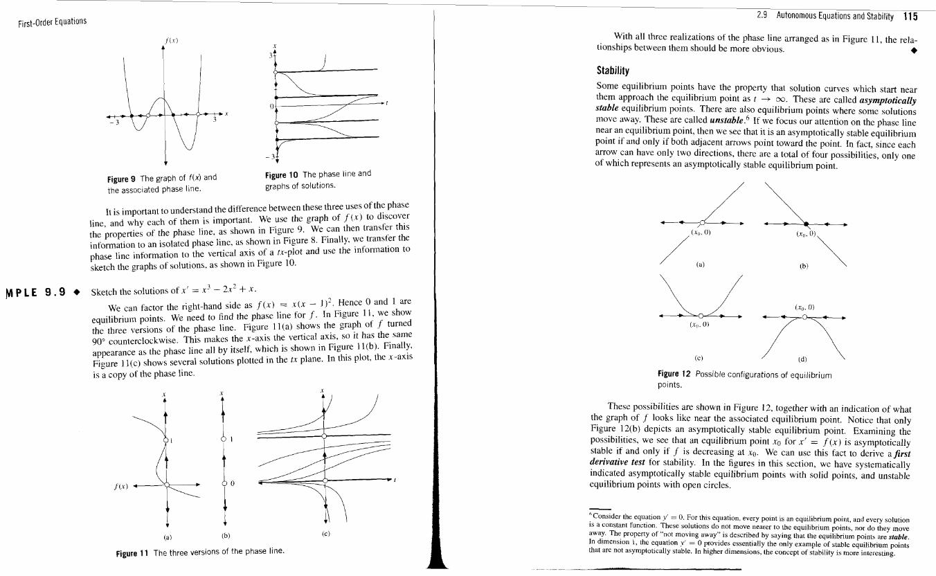
First-Order Equations
Figure 9 The graph of f ( x ) and Figure 10 The phase line and
the associated phase line. graphs of solutions.
It is important to understand the difference between these three uses of the phase line, and why each of them is important. We use the graph of f (x) to discover the properties of the phase line, as shown in Figure 9 We can then transfer this information to an isolated phase line, as shown in Figure 8 Finally. we transfer the nhaqe line information to the vertical axis of a ix-plot and use the information to -
sketch the graphs of solutions, as shown in Figure 10.
M P L E 9 . 9 + Sketch the solutions of x' = x' - 2x2 + X.
We can factor the right-hand side as f (x) = .x(x - I)'. Hence 0 and 1 are equilibrium points. We need to find the phase line for f . In Figure 1 I, we show the three versions of the phase line. Figure l l (a ) shows the graph of f turned 90" counterclockwise. This makes the x-axis the vertical axis, so it has the same appearance as the phase line all by itself, which is shown in Figure 1 l ( b ) Finally. Figure 1 l(c) shows several solutions plotted in the tx plane. In this plot, the x-axis u
is a copy of the phase line.
(a) (b)
Figure 11 The three versions of the phase line.
2.9 Autonomous Equations and Stability 11 5
With all three realizations of the phase line arranged as in Figure 11, the rela- tionships between them should be more obvious. + Stability Some equilibrium points have the property that solution curves which start near them approach the equilibrium point as r + co. These are called asymptotically stable equilibrium points. There are also equilibrium points where some solutions move away. These are called u n ~ t a b l e . ~ If we focus our attention on the phase line near an equilibrium point, then we see that it is an asymptotically stable equilibrium point if and only if both adjacent arrows point toward the point. In fact, since each arrow can have only two directions, there are a total of four possibilities, only one of which represents an asymptotically stable equilibrium point.
Figure 12 Possible configurations of equilibrium points.
These possibilities are shown in Figure 12, together with an indication of what the graph of f looks like near the associated equilibrium point. Notice that only Figure 12(b) depicts an asymptotically stable equilibrium point. Examining the possibilities, we see that an equilibrium point x o for x' = f (x) is asymptotically stable if and only if f is decreasing at xo. We can use this fact to derive afirst derivative test for stability. In the figures in this section, we have systematically indicated asymptotically stable equilibrium points with solid points, and unstable equilibrium points with open circles.
'Consider the equation y' = 0. For this equation. every point is an equilibrium point, and every solution is a constant function. These solutions do not move nearer to the equilibrium points, nor do they move away. The property of "not moving away" is described by saying that the equilibrium points are stable. In dimension I , the equation y' = 0 provides essentially the only example of stable equilibrium points that are not asymptotically stable. In higher dimensions, the concept of stability is more interesting.
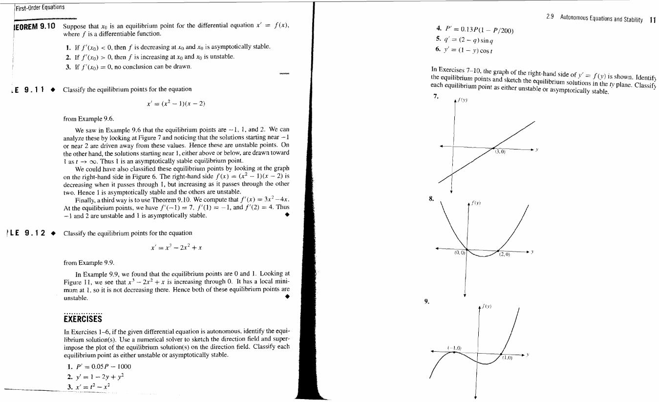
First-Order Equations I EOREM 9.10 Suppose that xo is an equilibrium point for the differential equation x' = f (x),
where f is a differentiable function. I
1. If fl(xo) < 0, then f is decreasing at no and xo is asymptotically stable.
2. If f '(no) > 0, then f i s increasing at no and xo is unstable.
3. If f '(xo) = 0, no conclusion can be drawn. ,-
, E 9 . 1 1 + Classify the equilibrium points for the equation
from Example 9.6.
We saw in Example 9.6 that the equilibrium points are -1, 1, and 2. We can analyze these by looking at Figure 7 and noticing that the solutions starting near - 1 or near 2 are driven away from these values. Hence these are unstable points. On the other hand, the solutions starting near 1, either above or below, are drawn toward 1 as t -+ CQ. Thus 1 is an asymptotically stable equilibrium point.
We could have also classified these equilibrium points by looking at the graph on the right-hand side in Figure 6. The right-hand side f (x) = (x2 - l)(x - 2) is decreasing when it passes through 1, but increasing as it passes through the other two. Hence 1 is asymptotically stable and the others are unstable.
Finally, a third way is to use Theorem 9.10. We compute that f '(x) = 3x2 -4x. At the equilibrium points, we have f '(- I ) = 7 . f '(1) = - 1, and f '(2) = 4. Thus - 1 and 2 are unstable and 1 is asymptotically stable. +
1 L E 9 . 1 2 6 Classify the equilibrium points for the equation
from Example 9.9.
In Example 9.9, we found that the equilibrium points are 0 and 1. Looking at Figure 11, we see that n3 - 2x2 + x is increasing through 0. It has a local rnini- mum at 1, so it is not decreasing there. Hence both of these equilibrium points are unstable. + ................ EXERCISES In Exercises 1-6, if the given differential equation is autonomous, identify the equi- librium solution(s). Use a numerical solver to sketch the direction field and super- impose the plot of the equilibrium solution(s) on the direction field. Classify each equilibrium point as either unstable or asymptotically stable.
1. P' = 0.05P - 1000
2. y' = 1 - 2y + y2
2.9 Autonolnous Equations a n d Stability 11 4. P' = 0.13 P ( l - P/200)
5. 9' = ( 2 - q ) sin q
6. y' = (1 - y ) cos t
In Exercises 7-10, the graph of the right-hand side of g' = f (g) is shown. Identifl the equilibrium points and sketch the equilibrium solutions in the tv plane. Classifi each equilibrium point as either unstable or asymptotically stable.
7. f
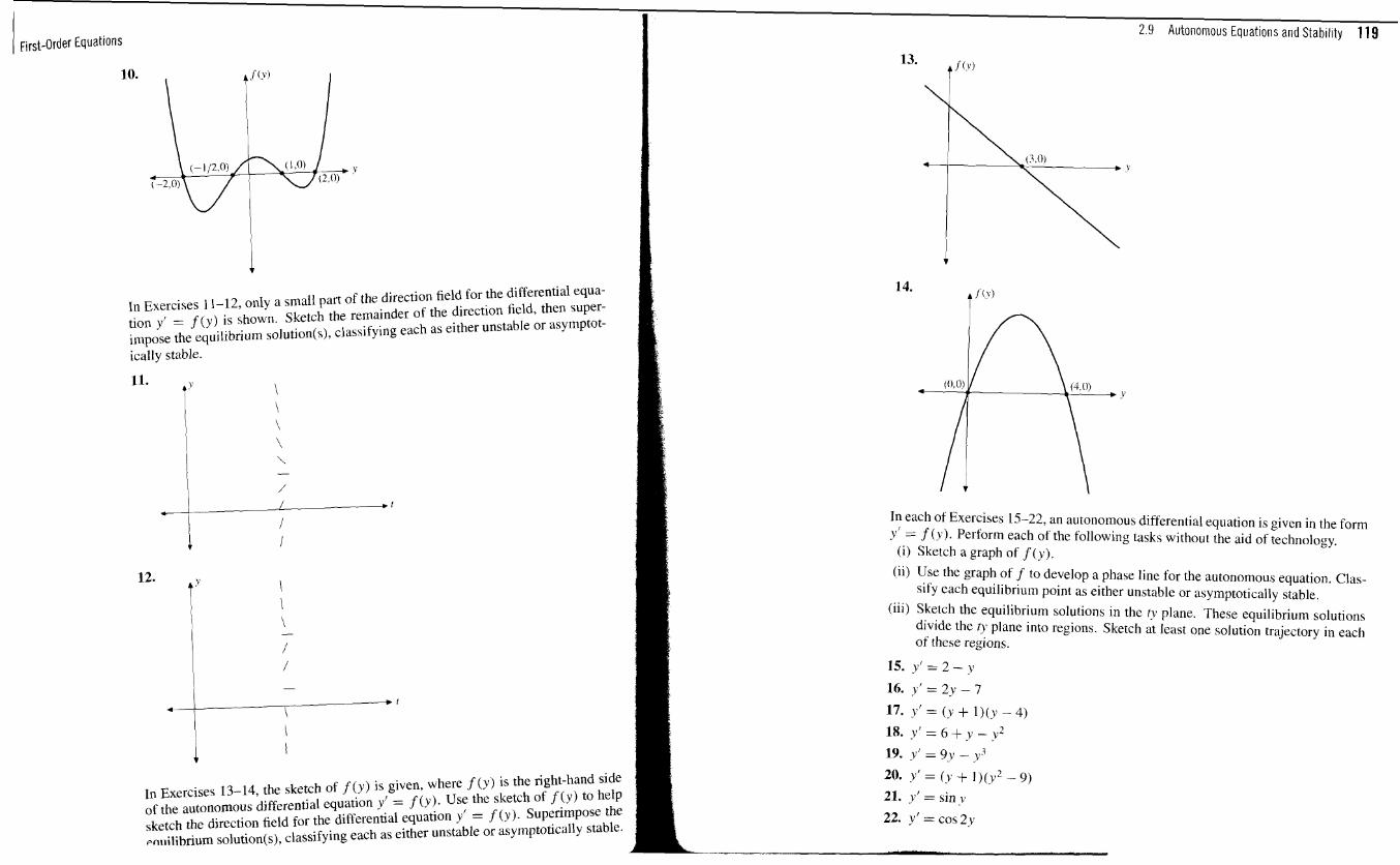
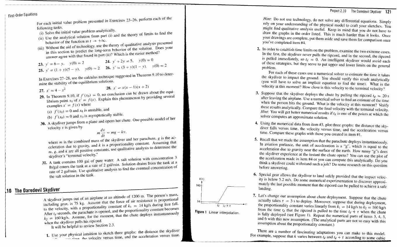
First-Order Equations
fir each initial value problem presented in Exercises 23-26. perform each the
following tasks. (i) Solve the initial value problem analytically.
(ii) Use the analytical solution from part (i) and the theory of limits to find the behavior of the function as t -+ 4-00.
(iii) Without the aid of technology. use the thcoly of qualitative analyds ~rewnted in this senion to predict the long-tern behavior of the solution. Does Your answer agree with that found in part (ii)? Which is the easier method?
23. y' = 6 - y , y(0) = 2 24. y' + 2y = 5 , y (0) = 0
25. v' = (1 + y ) ( 5 - y). ~ ' ( 0 ) = 2 Y (0) = 2 26. y' = (3 i- y)(l - Y ) . .
In Exercises 27-28, use the calculus technique suggesed in Theorem 9.10 to deter- mine the stability of the equilibrium solutions. -,
27. x' = 4 - x 2 28. x' = x(x - l)(x + 2 )
29. In Theorem 9.10, if f ' (re) = 0, no conclusion can be drawn about the equi- librium point xo of r' = f ( x ) . Explain this phenomenon by providing several
(a) f ' ( x o ) = 0 and xu is unstable, and (b) f '(x,,) = 0 and xo is asymptotically stable.
30. A skydiver jumps from a plane and opens her chutc. One possible model of her velocity u is given by dv
m y =mg - k v , d t
where m is the combined mass of the skydiver and her parachute. g is the ac- celeration due to gravity, and 1 is a proportionality constant. Assuming that nl, a, and k are all positive constants, use qualitative analysis to determine the skydiver's "terminal velocity."
-
31. A tank contains 100 gal of pure water. A salt solution with concentration 3 lblgal enters the tank at a rate of 2 gallmin. Solution drains from the tank at a rate of 2 gallmi*. Use qualitative analysis to find the eventual concentration of the salt solution in the tank.
.I0 The Daredevil Skydiver
A skydiver jumps out of an airplane at a11 altitude of 1200 m. The person's mass, including gear, is 75 kg. Assume that the force of air resistance is proportional to the velocity, with a proportionality constant of ki = 14 kgls during free fdl. After rd seconds, the parachute is opened, and the propurtionrlity constant becomes 1. = If50 kg/s Assume, for the moment, that the chute deploys instantaneousl~ 'L' - - - ~ u
whcn the skydiver pulls his ripcord. It will be helpful to review Section 2.3.
1. Use your physical intuition to sketch three graphs: the distance the skydiver ~ - - - - : +he ~ ~ l o c i t ~ versus time, and the acceleratio~l versus time.
I Project 2.10 The Daredevil Skydiver 121
HWt: Do not use technology, do not solve any differential equations. Simply rely on your understanding of the phyacal model to craft your sketches. You might find qualitative analysis useful. Keep in mind that you do not have to draw the graphs in the order listed. This is much harder than it hoks. Once your drawings are complete, put them aside and save them for comparison once you've completed item #4.
2. In order to establish time limits on the problem, examine the two extreme cases. In the first, the skydiver never pulls the ripcord, and in the second, the ripcord is pulled immediately, so t d = 0. An intelligent skydiver would avoid each of these strategies, but they serve to put upper and lower limits on the general problem.
For each of these cases use a numerical solver to estimate the time it takes the skydiver to impact the ground. You should verify this result analytically (you will have to solve an implicit equation to find the time). What is the velocity at this moment? How close is this velocity to the terminal velocity?
3. Suppose that the skydiver deploys the chute by pulling the ripcord td = 20 s after leaving the airplane. Use a numerical solver to find an estimate of thc time when the person hits the ground. What is the velocity at this moment? Verify thesc rcsults al~alytically. Compare the final velocity with the terminal velocity. H i n t : You will get better numerical results if td is one of the points at which the solver computes an approximate solution.
4. Using the numerical data from item #3, plot three graphs: the distance the sky- diver falls versus time. the velocity versus time, and the acceleration versus time. Compare these graphs with those you created in item #l.
5. Recall that we made the assumption that the parachute deploys instantaneously. In aviation parlance, the unit of accclcration is a "g", which is equal to the acceleration due to gravity near the surface of the earth. How many "g"s does the skydiver experience at the instant the chute opens? You can use the plot of the accelcration made in item #4 or you can compute this analytically. Do you think a skydiver could withstand such a jolt? Do some research on this question before answering.
6. Special gear allows the skydiver to land safely provided that the impact veloc- k ( r ) ity is below 5.2 d s . Do some numerical experimentation to discover approxi-
mately thc last possible moment that the ripcord can be pulled to achieve a safe
/--- landing. 7. Let's change our assumption about chute deployment. Suppose that the chute
14 actually takes r = 3 s to deploy. Moreover, suppose that during deployment, t the proportionality constant varies linearly from ki = 14 kg/s to kz = 160 kgis
from the time t d that the ripcord is pulled to the time td + r when the chute I Figure 1 Linear interpolation.
is fully deployed (see Figure 1). Repeat the numerical parts of items 3, 4. 5, and 6 with this new assumption. (The analytical parts are not so easy with this assumption about the proportionality constant.)
There are a number of fascinating adaptations you can make to this model. For example, suppose that k varies between td and td + r according to some cubic
first-Order Equations
interpolation. Or, suppose that the skydiver started at a higher altitude and you take the density of the air into account when determining the force of resistance.
Finally, there are a number of useful articles that will aid in your pursuit of this model. . Drucker, I., Minimal time of descent, The College Mathematics Journal, 26 . ~
(1995), pp. 252-235. ~ ~ ~ d ~ . D.B., ODE Models for the Parachute Problem, SIAM Review, 40 - A . - . . - ,
(1998), pp. 327-332. . Melka and Famior, Explorution of the parachute problem with STELLA. Newsletter for the Consortium for Ordinary Differential Equations Ex~ef i - ments, Sumrner-Fall, 1995
Modding and Applications T h e discovery of the calculus occurred at the beginning of the scientific revolution in the seventeenth century. This discovery was not a side issue in the revolution. Rather, it was the linchpin on which much of what followed was based. For the first time, humanlund had a systematic way to study how things changed. In many cases, the study of change has led to a differential equation, or to a system of differential equations through the process known as modeling.
We have explored a few applications, and we have constructed the correspond- ing models in Chapter 2. In this chapter, we will look carefully at the modeling process itself. The process will then be used in several applications. Along the way, we will also consider some examples of modeling that are faulty.
The main idea in the modeling process is explained easily. Suppose x is a quantity that varies with respect to the variable t . We want to model how it changes. From the mathematical point of view, the rate of change of x is the derivative
Building a model of the process involves finding an alternate expression for the rate of change of x as a function of t and x , say f ( t , x) . This leads us to the differential equation
This equation is the mathematical model of the process. The problem, of course, is discovering how the rate of change varies, and this
means discovering the function f ( t , x ) . Let's look at some examples.