INTRODUCTION TO DESCRIPTIVE SET THEORY

ANUSH TSERUNYAN

Mathematicians in the early 20th century discovered that the Axiom of Choice implied theexistence of pathological subsets of the real line lacking desirable regularity properties (forexample nonmeasurable sets). This gave rise to descriptive set theory, a systematic study ofclasses of sets where these pathologies can be avoided, including, in particular, the definablesets. In the first half of the course, we will use techniques from analysis and set theory, aswell as infinite games, to study definable sets of reals and their regularity properties, such asthe perfect set property (a strong form of the continuum hypothesis), the Baire property,and measurability.

Descriptive set theory has found applications in harmonic analysis, dynamical systems,functional analysis, and various other areas of mathematics. Many of the recent applicationsare via the theory of definable equivalence relations (viewed as sets of pairs), which providesa framework for studying very general types of classification problems in mathematics. Thesecond half of this course will give an introduction to this theory, culminating in a famousdichotomy theorem, which exhibits a minimum element among all problems that do notadmit concrete classification.

Acknowledgements. These notes owe a great deal to [Kec95]; in fact, some sections are almostliterally copied from it. Also, the author is much obliged to Anton Bernshteyn, Lou van den Dries,Nigel Pynn-Coates, and Jay Williams for providing dense sets of corrections and suggestions, whichsignificantly improved the readability and quality of these notes.

Contents

Part 1. Polish spaces 41. Definition and examples 42. Trees 6

2.A. Set theoretic trees 62.B. Infinite branches and closed subsets of AN 62.C. Compactness 72.D. Monotone tree-maps and continuous functions 8

3. Compact metrizable spaces 93.A. Basic facts and examples 93.B. Universality of the Hilbert Cube 103.C. Continuous images of the Cantor space 103.D. The hyperspace of compact sets 11

4. Perfect Polish spaces 134.A. Embedding the Cantor space 144.B. The Cantor–Bendixson Theorem, Derivatives and Ranks 15

1

2

5. Zero-dimensional spaces 165.A. Definition and examples 165.B. Luzin schemes 175.C. Topological characterizations of the Cantor space and the Baire space 175.D. Closed subspaces of the Baire space 185.E. Continuous images of the Baire space 18

6. Baire category 196.A. Nowhere dense sets 196.B. Meager sets 196.C. Relativization of nowhere dense and meager 206.D. Baire spaces 20

Part 2. Regularity properties of subsets of Polish spaces 227. Infinite games and determinacy 22

7.A. Non-determined sets and AD 237.B. Games with rules 23

8. The perfect set property 248.A. The associated game 24

9. The Baire property 259.A. The definition and closure properties 259.B. Localization 269.C. The Banach category theorem and a selector for =∗ 279.D. The Banach–Mazur game 299.E. The Kuratowski–Ulam theorem 309.F. Applications 32

10. Measurability 3310.A. Definitions and examples 3310.B. The null ideal and measurability 3410.C. Non-measurable sets 3510.D. The Lebesgue density topology on R 35

Part 3. Definable subsets of Polish spaces 3711. Borel sets 37

11.A. σ-algebras and measurable spaces 3711.B. The stratification of Borel sets into a hierarchy 3811.C. The classes Σ0

ξ and Π0ξ 40

11.D. Universal sets for Σ0ξ and Π0

ξ 4011.E. Turning Borel sets into clopen sets 42

12. Analytic sets 4312.A. Basic facts and closure properties 4412.B. A universal set for Σ1

1 4412.C. Analytic separation and Borel = ∆1

1 4512.D. Souslin operation A 46

13. More on Borel sets 4813.A. Closure under small-to-one images 4813.B. The Borel isomorphism theorem 50

3

13.C. Standard Borel spaces 5013.D. The Effros Borel space 5113.E. Borel determinacy 52

14. Regularity properties of analytic sets 5314.A. The perfect set property 5414.B. The Baire property and measurability 5614.C. Closure of BP and MEAS under the operation A 56

15. The projective hierarchy 5816. Γ-complete sets 60

16.A. Σ0ξ- and Π0

ξ-complete sets 60

16.B. Σ11-complete sets 61

Part 4. Definable equivalence relations, group actions and graphs 6317. Examples of equivalence relations and Polish group actions 64

17.A. Equivalence relations 6417.B. Polish groups 6517.C. Actions of Polish groups 66

18. Borel reducibility 6719. Perfect set property for quotient spaces 68

19.A. Co-analytic equivalence relations: Silver’s dichotomy 6919.B. Analytic equivalence relations: Burgess’ trichotomy 6919.C. Meager equivalence relations: Mycielski’s theorem 70

20. Concrete classifiability (smoothness) 7120.A. Definitions 7120.B. Examples of concrete classification 7220.C. Characterizations of smoothness 7420.D. Nonsmooth equivalence relations 7420.E. General Glimm–Effros dichotomies 7620.F. Proof of the Becker–Kechris dichotomy 77

21. Definable graphs and colorings 7921.A. Definitions and examples 7921.B. Chromatic numbers 8021.C. G0—the graph cousin of E0 8221.D. The Kechris–Solecki–Todorcevic dichotomy 83

22. Some corollaries of the G0-dichotomy 8322.A. Proof of Silver’s dichotomy 8322.B. Proof of the Luzin–Novikov theorem 8422.C. The Feldman–Moore theorem and E∞ 84

References 85

4

Part 1. Polish spaces

1. Definition and examples

Definition 1.1. A topological space is called Polish if it is separable and completely metri-zable (i.e. admits a complete compatible metric).

We work with Polish topological spaces as opposed to Polish metric spaces because wedon’t want to fix a particular complete metric, we may change it to serve different purposes;all we care about is that such a complete compatible metric exists. Besides, our maps arehomeomorphisms and not isometries, so we work in the category of topological spaces andnot metric spaces.

Examples 1.2.

(a) For all n ∈ N, n = {0, 1, ..., n− 1} is Polish with discrete topology; so is N;

(b) Rn and Cn, for n ≥ 1;

(c) Separable Banach spaces; in particular, separable Hilbert spaces, `p(N) and Lp(R) for0 < p <∞.

The following lemma, whose proof is left as an exercise, shows that when working withPolish spaces, we may always take a complete compatible metric d ≤ 1.

Lemma 1.3. If X is a topological space with a compatible metric d, then the following metricis also compatible: for x, y ∈ X, D(x, y) = min(d(x, y), 1).

Proposition 1.4.

(a) Completion of any separable metric space is Polish.(b) A closed subset of a Polish space is Polish (with respect to relative topology).(c) A countable disjoint union1 of Polish spaces is Polish.(d) A countable product of Polish spaces is Polish (with respect to the product topology).

Proof. (a) and (b) are obvious. We leave (c) as an exercise and prove (d). To this end, letXn, n ∈ N be Polish spaces and let dn ≤ 1 be a complete compatible metric for Xn. Forx, y ∈

∏n∈NXn, define

d(x, y) ..=∑n∈N

2−ndn(x(n), y(n)).

It is easy to verify that d is a complete compatible metric for the product topology on∏n∈NXn. �

Examples 1.5.

(a) RN, CN;

(b) The Cantor space C ..= 2N, with the discrete topology on 2;

1Disjoint union of topological spaces {Xi}i∈I is the space⊔i∈I Xi

..=⋃i∈I {i} ×Xi equipped with the

topology generated by sets of the form {i} × Ui, where i ∈ I and Ui ⊆ Xi is open.

5

(c) The Baire space N ..= NN, with the discrete topology on N.

(d) The Hilbert cube IN, where I = [0, 1].

As mentioned in the previous proposition, closed subsets of Polish spaces are Polish. Whatother subsets have this property? The proposition below answers this question, but first werecall here that countable intersections of open sets are called Gδ sets, and countable unionsof closed sets are called Fσ.

Lemma 1.6. If X is a metric space, then closed sets are Gδ; equivalently, open sets are Fσ.

Proof. Let C ⊆ X be a closed set and let d be a metric for X. For ε > 0, define Uε ..={x ∈ X : d(x,C) < ε}, and we claim that C =

⋂n U1/n. Indeed, C ⊆

⋂n U1/n is trivial, and

to show the other inclusion, fix x ∈⋂n U1/n. Thus, for every n, we can pick xn ∈ C with

d(x, xn) < 1/n, so xn → x as n→∞, and hence x ∈ C by the virtue of C being closed. �

Proposition 1.7. A subset of a Polish space is Polish if and only if it is Gδ.

Proof. Let X be a Polish space and let dX be a complete compatible metric on X.⇐: Considering first an open set U ⊆ X, we exploit the fact that it does not contain itsboundary points to define a compatible metric for the topology of U that makes the boundaryof U “look like infinity” in order to prevent sequences that converge to the boundary frombeing Cauchy. In fact, instead of defining a metric explicitly2, we define a homeomorphism ofU with a closed subset of X × R by

x 7→(x,

1

dX(x, ∂U)

),

where dX is a complete compatible metric for X. It is, indeed, easy to verify that this map isan embedding and its image is closed.

Combining countably-many instances of this gives a proof for Gδ sets: given Y ..=⋂n∈N Un

with Un open, the map Y → X × RN defined by

x 7→(x,

(1

dX(x, ∂Un)

)n

)is a homeomorphism of Y with a closed subset of X × RN.⇒ (Alexandrov): Let Y ⊆ X be completely metrizable and let dY be a complete compatiblemetric for Y . Define an open set Vn ⊆ X as the union of all open sets U ⊆ X that satisfy

(i) U ∩ Y 6= ∅,(ii) diamdX (U) < 1/n,(iii) diamdY (U ∩ Y ) < 1/n.

We show that Y =⋂n∈N Vn. First fix x ∈ Y and take any n ∈ N. Take an open neighborhood

U1 ⊆ Y of x in Y of dY -diameter less than 1/n. By the definition of relative topology, thereis an open set U2 in X such that U2 ∩ Y = U1. Let U3 be an open neighborhood of x in X ofdX-diameter less than 1/n. Then U = U2 ∩ U3 satisfies all of the conditions above. Hencex ∈ Vn.

Conversely, if x ∈⋂n∈N Vn, then for each n ∈ N, there is an open (relative to X)

neighborhood Un ⊆ X of x satisfying the conditions above. Condition (ii) implies that x ∈ Y ,so any open neighborhood of x has a nonempty intersection with Y ; because of this, we can

2This version of the proof was suggested by Anton Bernshteyn.

6

replace Un by⋂m≤n Um and assume without loss of generality that (Un)n∈N is decreasing.

Now, take xn ∈ Un ∩ Y . Conditions (i) and (ii) imply that (xn)n∈N converges to x. Moreover,condition (iii) and the fact that (Un)n∈N is decreasing imply that (xn)n∈N is Cauchy withrespect to dY . Thus, since dY is complete, xn → x′ for some x′ ∈ Y . Because limit is uniquein Hausdorff spaces, x = x′ ∈ Y . �

As an example of a Gδ subset of a Polish space, we give the following proposition, whoseproof is left to the reader.

Proposition 1.8. The Cantor space C is homeomorphic to a closed subset of the Baire spaceN , whereas N is homeomorphic to a Gδ subset of C.

2. Trees

2.A. Set theoretic trees. For a nonempty set A, we denote by A<N the set of finite tuplesof elements of A, i.e.

A<N =⋃n∈N

An,

where A0 = {∅}. For s ∈ A<N, we denote by |s| the length of s; thus, s is a function from{0, 1, ..., |s| − 1} to A. Recalling that functions are sets of pairs, the notation s ⊆ t fors, t ∈ A<N means that |s| ≤ |t| and s(i) = t(i) for all i < |s|.Definition 2.1. For a set A, a subset T of A<N is called a (set theoretic) tree if it is closeddownward under ⊆, i.e. for all s, t ∈ A<N, if t ∈ T and s ⊆ t, then s ∈ T .

For s ∈ A<N and a ∈ A, we write saa to denote the extension of s to a tuple of length|s| + 1 that takes the value a at index |s|. For s, t ∈ A<N, we also write sat to denote thetuple obtained by appending t at the end of s.

To see why the sets T in the above definitions are called trees, we now show how to obtaina graph theoretic rooted tree GT from a set theoretic tree T . Define the vertex set of GT tobe T . Note that since T is nonempty, ∅ ∈ T , and declare ∅ the root of GT . Now put an edgebetween s, t ∈ T if t = saa for some a ∈ A.

Conversely, given a graph theoretic rooted tree G (a connected acyclic graph) with rootv0, one obtains a set theoretic tree TG on V (G) (the set of vertices of G) by identifying eachvertex v with (v1, ..., vn), where vn = v and (v0, v1, ..., vn) is the unique path from v0 to v.

2.B. Infinite branches and closed subsets of AN. Call a tree T on A pruned if for everys ∈ T , there is a ∈ A with saa ∈ T .

Given a tree T on a set A, we denote by [T ] the set of infinite branches through T , that is,

[T ] ={x ∈ AN : ∀n ∈ N(x|n ∈ T )

}.

Thus we obtain a subset of AN from a tree. Conversely, given a subset Y ⊆ AN, we canobtain a tree TY on A by:

TY = {x|n : x ∈ Y, n ∈ N} .Note that TY is a pruned tree. It is also clear that Y ⊆ [TY ], but for which subsets Y do wehave [TY ] = Y ? To answer this question, we give A the discrete topology and consider AN asa topological space with the product topology. Note that the sets of the form

Ns..={x ∈ AN : s ⊆ x

},

for s ∈ A<N, form a basis for the product topology on AN.

7

Lemma 2.2. For a tree T on A, [T ] is a closed subset of AN.

Proof. We show that the complement of [T ] is open. Indeed, if x /∈ [T ], then there is n ∈ Nsuch that s = x|n /∈ T . But then Ns ∩ [T ] = ∅. �

Proposition 2.3. A subset Y ⊆ AN is closed if and only if Y = [TY ].

Proof. The right-to-left direction follows form the previous lemma, so we prove left-to-right.Let Y be closed, and as Y ⊆ [TY ], we only need to show [TY ] ⊆ Y . Fix x ∈ [TY ]. By thedefinition of TY , for each n ∈ N, there is yn ∈ Y such that x|n ⊆ yn. It is clear that (yn)n∈Nconverges pointwise to x (i.e. converges in the product topology) and hence x ∈ Y since Y isclosed. �

Note that if A is countable, then AN is Polish. Examples of such spaces are the Cantorspace and the Baire space, which, due to their combinatorial nature, are two of the most usefulPolish spaces in descriptive set theory. We think of the Cantor space and the Baire space asthe sets of infinite branches through the complete binary and N-ary trees, respectively. Treeson N in particular play a crucial role in the subject, as we will see below.

2.C. Compactness. Above, we characterized the closed subsets of AN as the sets of infinitebranches through trees on A. Here we characterize the compact subsets.

For a tree T on A, and s ∈ T , put

T (s) ..={a ∈ A : saa ∈ T

}.

We say that a tree T on A is finitely branching if for each s ∈ T , T (s) is finite. Equivalently,in GT every vertex has finite degree.

Lemma 2.4 (Konig). Any finitely branching infinite tree T on A has an infinite branch, i.e.[T ] 6= ∅.

Proof. Very easy, left to the reader. �

For a tree T ⊆ A<N, sets of the form Ns ∩ [T ], for s ∈ A<N, form a basis for the relativetopology on [T ]. Also, for s ∈ A<N, putting Ts ..= {t ∈ T : t ⊆ s ∨ t ⊇ s}, it is clear that Tsis a tree and [Ts] = Ns ∩ [T ].

Proposition 2.5. For a tree T ⊆ A<N, if T is finitely branching, then [T ] is compact. For apruned tree T ⊆ A<N, the converse also holds: if [T ] is compact, then T is finitely branching.Thus, a closed set Y ⊆ AN is compact if and only if TY is finitely branching.

Proof. We leave proving the first statement as an exercise. For the second statement, letT be a pruned tree and suppose that [T ] is compact. Assume for contradiction that T isnot finitely branching, i.e. there is s ∈ T such that T (s) is infinite. Since [T ] is compact, sois [Ts] being a closed subset, so we can focus on [Ts]. For each a ∈ T (s), the set [Tsaa] isnonempty because T is pruned. But then {[Tsaa]}a∈T (s) is an open cover of [Ts] that doesn’thave a finite subcover since the sets in it are nonempty and pairwise disjoint. �

A subset of a topological space is called σ-compact or Kσ if it is a countable union ofcompact sets. The above proposition shows that the Baire space is not compact. In fact, wehave something stronger:

Corollary 2.6. The Baire space N is not σ-compact.

8

Proof. For x, y ∈ N , we say that y eventually dominates x, if y(n) ≥ x(n) for sufficientlylarge n. Let (Kn)n∈N be a sequence of compact subsets of N . By the above proposition, TKn

is finitely branching and hence there is xn ∈ N that eventually dominates every element ofKn. By diagonalization, we obtain x ∈ N that eventually dominates xn for all n ∈ N. Thus,x eventually dominates every element of

⋃n∈NKn, and hence, the latter cannot be all of

N . �

The Baire space is not just an example of a topological space that is not σ-compact, it isin fact the canonical obstruction to being σ-compact as the following dichotomy shows:

Theorem 2.7 (Hurewicz). For any Polish space X, either X is σ-compact, or else, Xcontains a closed subset homeomorphic to N .

We will not prove this theorem here since its proof is somewhat long and we will not beusing it below.

2.D. Monotone tree-maps and continuous functions. In this subsection, we show howto construct continuous functions between tree spaces (i.e. spaces of infinite branches throughtrees).

Definition 2.8. Let S, T be trees (on sets A,B, respectively). A map ϕ : S → T is calledmonotone if s ⊆ t implies ϕ(s) ⊆ ϕ(t). For such ϕ let

Dϕ ={x ∈ [S] : lim

n→∞|ϕ(x|n)| =∞

}.

Define ϕ∗ : Dϕ → [T ] by letting

ϕ∗(x) ..=⋃n∈N

ϕ(x|n).

We call ϕ proper if Dϕ = [S].

Proposition 2.9. Let ϕ : S → T be a monotone map (as above).

(a) The set Dϕ is Gδ in [S] and ϕ∗ : Dϕ → [T ] is continuous.(b) Conversely, if f : G→ [T ] is continuous, with G ⊆ [S] a Gδ set, then there is monotone

ϕ : S → T with f = ϕ∗.

Proof. The proof of (b) is outlined as a homework problem, so we will only prove (a) here.To see that Dϕ is Gδ note that for x ∈ [S], we have

x ∈ Dϕ ⇐⇒ ∀n∃m|ϕ(x|m)| ≥ n,

and the set Un,m = {x ∈ [S] : |ϕ(x|m)| ≥ n} is trivially open as membership in it dependsonly on the first m coordinates. For the continuity of ϕ∗, it is enough to show that for eachτ ∈ T , the preimage of [Tτ ] under ϕ∗ is open; but for x ∈ Dϕ,

x ∈ (ϕ∗)−1([Tτ ])⇔ ϕ∗(x) ∈ [Tτ ]

⇔ ϕ∗(x) ⊇ τ

⇔ (∃σ ∈ S with ϕ(σ) ⊇ τ) x ∈ Sσ,

and in the latter condition, ∃ is a union, and x ∈ Sσ defines a basic open set. �

9

Using this machinery, we easily derive the following useful lemma.A closed set C in a topological space X is called a retract of X if there is a continuous

function f : X → C such that f |C = id |C (i.e. f(x) = x, for all x ∈ C). This f is called aretraction of X to C.

Lemma 2.10. Any nonempty closed subset X ⊆ AN is a retract of AN. In particular, forany two nonempty closed subsets X ⊆ Y , X is a retract of Y .

Proof. Noting that TX is a nonempty pruned tree, we define a monotone map ϕ : A<N → TXsuch that ϕ(s) = s for s ∈ TX and thus ϕ∗ will be a retraction of AN to X. For s ∈ A<N, wedefine ϕ(s) by induction on |s|. Let ϕ(∅) ..= ∅ and assume ϕ(s) is defined. Fix a ∈ A. Ifsaa ∈ TX , put ϕ(saa) ..= saa. Otherwise, there is b ∈ A with ϕ(s)ab ∈ TX because TX ispruned, and we put ϕ(saa) ..= ϕ(s)ab. �

3. Compact metrizable spaces

3.A. Basic facts and examples. Recall that a topological space is called compact if everyopen cover has a finite subcover. By taking complements, this is equivalent to the statementthat every (possibly uncountable) family of closed sets with the finite intersection property3

has a nonempty intersection. In the following proposition we collect basic facts about compactspaces, which we won’t prove (see Sections 0.6, 4.1, 4.2, 4.4 of [Fol99]).

Proposition 3.1.

(a) Closed subsets of compact topological spaces are compact.(b) Compact (in the relative topology) subsets of Hausdorff topological spaces are closed.(c) Union of finitely many compact subsets of a topological space is compact. Finite sets are

compact.(d) Continuous image of a compact space is compact. In particular, if f : X → Y is

continuous, where X is compact and Y is Hausdorff, then f maps closed (resp. Fσ) setsto closed (resp. Fσ) sets.

(e) A continuous injection from a compact space into a Hausdorff space is an embedding(i.e. a homeomorphism with the image).

(f) Disjoint union of finitely many compact spaces is compact.(g) (Tychonoff’s Theorem) Product of compact spaces is compact.

Definition 3.2. For a metric space (X, d) and ε > 0, a set F ⊆ X is called an ε-net if anypoint in X is within ε distance from a point in F , i.e. X =

⋃y∈F B(y, ε), where B(y, ε) is

the open ball of radius ε centered at y. Metric space (X, d) is called totally bounded if forevery ε > 0, there is a finite ε-net.

Lemma 3.3. Totally bounded metric spaces are separable.

Proof. For every n, let Fn be a finite 1n-net. Then, D =

⋃n Fn is countable and dense. �

Proposition 3.4. Let (X, d) be a metric space. The following are equivalent:

(1) X is compact.(2) Every sequence in X has a convergent subsequence.(3) X is complete and totally bounded.

3We say that a family {Fi}i∈I of sets has the finite intersection property if for any finite I0 ⊆ I,⋂i∈I0 Fi 6= ∅.

10

In particular, compact metrizable spaces are Polish.

Proof. Outlined in a homework exercise. �

Examples of compact Polish spaces include C, T = R/Z, I = [0, 1], IN. A more advancedexample is the space P (X) of Borel probability measures on a compact Polish space X underthe weak∗-topology. In the next two subsections we will see however that the Hilbert cubeand the Cantor space play special roles among all the examples.

3.B. Universality of the Hilbert Cube.

Theorem 3.5. Every separable metrizable space embeds into the Hilbert cube IN. In particular,the Polish spaces are, up to homeomorphism, exactly the Gδ subspaces of IN, and the compactmetrizable spaces are, up to homeomorphism, exactly the closed subspaces of IN.

Proof. Let X be a separable metrizable space. Fix a compatible metric d ≤ 1 and a densesubset (xn)n∈N. Define f : X → IN by setting

f(x) ..=(d(x, xn)

)n∈N,

for x ∈ X. It is straightforward to show that f is injective and that f, f−1 are continuous. �

Corollary 3.6. Every Polish space can be embedded as a dense Gδ subset into a compactmetrizable space.

Proof. By the previous theorem, any Polish space is homeomorphic to a Gδ subset Y of theHilbert cube and Y is dense in its closure, which is compact. �

As we just saw, Polish spaces can be thought of as Gδ subsets of a particular Polish space.Although this is interesting on its own, it would be more convenient to have Polish spaces asclosed subsets of some Polish space because the set of closed subsets of a Polish space has anice structure, as we will see later on. This is accomplished in the following theorem.

Theorem 3.7. Every Polish space is homeomorphic to a closed subspace of RN.

Proof. Let X be a Polish space and, by the previous theorem, we may assume that X is aGδ subspace of IN. Letting d be a complete compatible metric on IN, we use a trick similarto the one used in Proposition 1.7 when we made a Gδ set “look closed” by changing themetric. Let X =

⋂n Un, where Un are open in IN, and put Fn = IN \ Un. Define f : X → RN

as follows: for x ∈ X,

f(x)(n) ..=

{x(k) if n = 2k

1d(x,Fk)

if n = 2k + 1.

Even coordinates ensure that f is injective and the odd coordinates ensure that the image isclosed. The continuity of f follows from the continuity of the coordinate functions x 7→ f(x)(n),for all n ∈ N. Thus, f is an embedding as IN is compact (see (e) of Proposition 3.1); in fact,f−1 is just the projection onto the even coordinates and hence is obviously continuous. �

3.C. Continuous images of the Cantor space. Theorem 3.5 characterizes all compactmetrizable spaces as closed subspaces of IN. Here we give another characterization usingsurjections instead of injections (reversing the arrows).

Theorem 3.8. Every nonempty compact metrizable space is a continuous image of C.

11

Proof. First we show that IN is a continuous image of C. For this it is enough to show that Iis a continuous image of C since C is homeomorphic to CN (why?). But the latter is easilydone via the map f : C → I given by

x 7→∑n

x(n)2−n−1.

Now let X be a compact metrizable space, and by Theorem 3.5, we may assume that X isa closed subspace of IN. As we just showed, there is a continuous surjection g : C → IN andthus, g−1(X) is a closed subset of C, hence a retract of C (Lemma 2.10). �

3.D. The hyperspace of compact sets. In this subsection we discuss the set of all compactsubsets of a given Polish space and give it a natural topology, which turns out to be Polish.

Notation 3.9. For a set X and a collection A ⊆P(X), define the following for each subsetU ⊆ X:

(U)A ..= {A ∈ A : A ⊆ U} ,[U ]A ..= {A ∈ A : A ∩ U 6= ∅} .

Now let X be a topological space. We denote by K(X) the collection of all compact subsetsof X and we equip it with the Vietoris topology, namely, the one generated by the sets of theform (U)K and [U ]K, for open U ⊆ X. Thus, a basis for this topology consists of the sets

〈U0;U1, ..., Un〉K ..=(U0)K ∩ [U1]K ∩ [U2]K ∩ ... ∩ [Un]K

= {K ∈ K(X) : K ⊆ U0 ∧K ∩ U1 6= ∅ ∧ ... ∧K ∩ Un 6= ∅} ,

for U0, U1, ..., Un open in X. By replacing Ui with Ui ∩U0, for i ≤ n, we may and will assumethat Ui ⊆ U0 for all i ≤ n.

Now we assume further that (X, d) is a metric space with d ≤ 1. We define the Hausdorffmetric dH on K(X) as follows: for K,L ∈ K(X), put

δ(K,L) ..= maxx∈K

d(x, L),

with convention that d(x, ∅) = 1 and δ(∅, L) = 0. Thus, lettingB(L, r) ..= {x ∈ X : d(x, L) < r},we have

δ(K,L) = infr

[K ⊆ B(L, r)].

δ(K,L) is not yet a metric because it is not symmetric. So we symmetrize it: for arbitraryK,L ∈ K(X), put

dH(K,L) = max {δ(K,L), δ(L,K)} .Thus,

dH(K,L) = infr

[K ⊆ B(L, r) and L ⊆ B(K, r)].

Proposition 3.10. Hausdorff metric is compatible with the Vietoris topology.

Proof. Left as an exercise. �

Proposition 3.11. If X is separable, then so is K(X).

12

Proof. Let D be a countable dense subset of X, and put

Fin(D) = {F ⊆ D : F is finite} .Clearly Fin(D) ⊆ K(X) and is countable. To show that it is dense, fix a nonempty basic openset 〈U0;U1, ..., Un〉K, where we may assume that ∅ 6= Ui ⊆ U0 for all i ≤ n. By density of D inX, there is di ∈ Ui∩D for each 1 ≤ i ≤ n, so {di : 1 ≤ i ≤ n} ∈ 〈U0;U1, ..., Un〉K∩Fin(D). �

Next we will study convergence in K(X). Given Kn → K, we will describe what K isin terms of Kn without referring to Hausdorff metric or Vietoris topology. To do this, wediscuss other notions of limits for compact sets.

Given any topological space X and a sequence (Kn)n∈N in K(X), define its topologicalupper limit, T limnKn to be the set

{x ∈ X : Every open nbhd of x meets Kn for infinitely many n} ,and its topological lower limit, T limnKn, to be the set

{x ∈ X : Every open nbhd of x meets Kn for all but finitely many n} .It is immediate from the definitions that T limnKn ⊆ T limnKn and both sets are closed (butmay not be compact). It is also easy to check that

T limnKn =⋂i∈N

⋃j≥i

Kj.

If T limnKn = T limnKn, we call the common value the topological limit of (Kn)n∈N, anddenote it by T limnKn. If d ≤ 1 is a compatible metric for X, then one can check (left as anexercise) that Kn → K in Hausdorff metric implies K = T limnKn. However, the conversemay fail as the following examples show.

Examples 3.12.

(a) Let X = Rm and Kn = B(~0, 1 + (−1)n

n). Then Kn → B(~0, 1) in Hausdorff metric.

(b) Let X = R and Kn = [0, 1] ∪ [n, n+ 1]. The Hausdorff distance between different Kn is1, so the sequence (Kn)n does not converge in Hausdorff metric. Nevertheless T limnKn

exists and is equal to [0, 1].

(c) Let X = R, K2n = [0, 1] and K2n+1 = [1, 2], for each n ∈ N. In this case, we have

T limnKn = [0, 2], whereas T limnKn = {1}.Finally, note that if X is first-countable (for example, metrizable) and Kn 6= ∅ then the

topological upper limit consists of all x ∈ X that satisfy:

∃(xn)n∈N[∀n(xn ∈ Kn) and xni→ x for some subsequence (xni

)i∈N],

and the topological lower limit consists of all x ∈ X that satisfy:

∃(xn)n∈N[∀n(xn ∈ Kn) and xn → x].

The relation between these limits and the limit in Hausdorff metric is explored morein homework problems. Here we just use the upper topological limit merely to prove thefollowing theorem.

Theorem 3.13. If X is completely metrizable then so is K(X). In particular, if X is Polish,then so is K(X).

13

Proof. Let d ≤ 1 be a complete compatible metric on X and let (Kn)n∈N be a Cauchysequence in K(X), where we assume without loss of generality that Kn 6= ∅. Setting

K = T limnKn =⋂N∈N

⋃n≥N Kn, we will show that K ∈ K(X) and dH(Kn, K)→ 0.

Claim. K is compact.

Proof of Claim. Since K is closed and X is complete, it is enough to show that K is totallybounded. For this, we will verify that given ε > 0 there is a finite set F ⊆ X such thatK ⊆ B(F, ε). Let N be such that dH(Kn, Km) < ε/4 for all n,m ≥ N , and let F be anε/4-net for KN , i.e. KN ⊆ B(F, ε/4). Thus, for each n ≥ N ,

Kn ⊆ B(KN , ε/4) ⊆ B(F, ε/4 + ε/4)

so⋃n≥N Kn ⊆ B(F, ε/2), and hence

K ⊆⋃n≥N

Kn ⊆ B(F, ε/2) ⊆ B(F, ε).

�

It remains to show that dH(Kn, K)→ 0. Fix ε > 0 and let N be such that dH(Kn, Km) <ε/2 for all n,m ≥ N . We will show that if n ≥ N , dH(Kn, K) < ε.

Proof of δ(K,Kn) < ε. By the choice of N , we have Km ⊆ B(Kn, ε/2) for each m ≥ N . Thus⋃m≥N Km ⊆ B(Kn, ε/2) and hence K ⊆

⋃m≥N Km ⊆ B(Kn, ε).

Proof of δ(Kn, K) < ε. Fix x ∈ Kn. Using the fact that (Km)m≥n is Cauchy, we can findn = n0 < n1 < ... < ni < ... such that dH(Kni

, Km) < ε2−(i+1) for all m ≥ ni. Then, definexni∈ Kni

as follows: xn0..= x and for i > 0, let xni

∈ Knibe such that d(xni

, xni+1) < ε2−(i+1).

It follows that (xni)i∈N is Cauchy, so xni

→ y for some y ∈ X. By the definition of K, y ∈ K.Moreover, d(x, y) ≤

∑∞i=0 d(xni

, xni+1) <

∑∞i=0 ε2

−(i+1) = ε. �

Proposition 3.14. If X is compact metrizable, so is K(X).

Proof. It is enough to show that if d is a compatible metric for X, with d ≤ 1, then (K(X), dH)is totally bounded. Fix ε > 0. Let F ⊆ X be a finite ε-net for X. Then it is easy to verifythat P(F ) is an ε-net for K(X), i.e. K(X) ⊆

⋃S⊆F BdH (S, ε). �

4. Perfect Polish spaces

Recall that a point x of a topological space X is called isolated if {x} is open; call x alimit point otherwise. A space is perfect if it has no isolated points. If P is a subset of atopological space X, we call P perfect in X if P is closed and perfect in its relative topology.For example, Rn, RN, Cn, CN, IN, C, N are perfect. Another example of a perfect space isC(X), where X compact metrizable.

Caution 4.1. Q is a perfect topological space, but it is not a perfect subset of R because itisn’t closed.

14

4.A. Embedding the Cantor space. The following definition gives a construction that isused when embedding the Cantor space.

Definition 4.2. A Cantor scheme on a set X is a family (As)s∈2<N of subsets of X suchthat:

(i) Asa0 ∩ Asa1 = ∅, for s ∈ 2<N;

(ii) Asai ⊆ As, for s ∈ 2<N, i ∈ {0, 1}.

If (X, d) is a metric space and we additionally have

(iii) limn→∞ diam(Ax|n) = 0, for x ∈ C,

we say that (As)s∈2<N has vanishing diameter. In this case, we let

D =

{x ∈ C :

⋂n∈N

Ax|n 6= ∅

}and define f : D → X by {f(x)} ..=

⋂Ax|n . This f is called the associated map. Note that f

is injective.

Theorem 4.3 (Perfect Set Theorem). Let X be a nonempty perfect Polish space. Then thereis an embedding of C into X.

Proof. Fix a complete compatible metric for X. Using that X is nonempty perfect, define aCantor scheme (Us)s∈2<N on X by induction on |s| so that

(i) Us is nonempty open;(ii) diam(Us) < 1/|s|;(iii) Usai ⊆ Us, for i ∈ {0, 1}.We do this as follows: let U∅ = X and assume Us is defined. Since X does not have isolatedpoints, Us must contain at least two points x 6= y. Using the fact that X is Hausdorff, taketwo disjoint open neighborhoods Usa0 3 x and Usa1 3 y with small enough diameter so thatthe conditions (ii) and (iii) above are satisfied. This finishes the construction.

Now let f : D → X be the map associated with the Cantor scheme. It is clear that D = Cbecause for x ∈ C,

⋂n∈N Ux|n =

⋂n∈N Ux|n 6= ∅ by the completeness of X. It is also clear that

f is injective, so it is enough to prove that it is continuous (since continuous injections fromcompact to Hausdorff are embeddings). To this end, let x ∈ C and, for ε > 0, take an openball B ⊆ X of radius ε around f(x). Because diam(Ux|n)→ 0 as n→∞ and f(x) ∈ Ux|n forall n, there is n such that Ux|n ⊆ B. But then

f(Nx|n) ⊆ Ux|n ⊆ B.

�

Corollary 4.4. Any nonempty perfect Polish space has cardinality continuum.

Corollary 4.5. For a perfect Polish space X, the generic compact subset of X is perfect.More precisely, the set

Kp(X) = {K ∈ K(X) : K is perfect}is a dense Gδ subset of K(X).

Proof. Left as a homework exercise. �

15

4.B. The Cantor–Bendixson Theorem, Derivatives and Ranks. The following theo-rem shows that Continuum Hypothesis holds for Polish spaces.

Theorem 4.6 (Cantor–Bendixson). Let X be a Polish space. Then X can be uniquely writtenas X = P ∪ U , with P a perfect subset of X and U countable open.

The perfect set P is called the perfect kernel of X.We will give two different proofs of this theorem. In both, we define a notion of smallness

for open sets and throw away the small basic open sets from X to get P . However, the smallopen sets in the first proof are “larger” than those in the second proof, and thus, in the firstproof, after throwing small basic open sets away once, we are left with no small open set,while in the second proof, we have to repeat this process transfinitely many times to get ridof all small open sets. This transfinite analysis provides a very clear picture of the structureof X and allows for defining notions of derivatives of sets and ranks.

Call a point x ∈ X a condensation point if it does not have a small open neighborhood, i.e.every open neighborhood of x is uncountable.

Proof of Theorem 4.6. We will temporarily call an open set small if it is countable. Let Pbe the set of all condensation points of X; in other words, P = X \ U , where U is the unionof all small open sets. Thus it is clear that P is closed and doesn’t contain isolated points.Also, since X is second countable, U is a union of countably many small basic open sets andhence, is itself countable. This finishes the proof of the existence.

For the uniqueness, suppose that X = P1 ∪ U1 is another such decomposition. Thus, bydefinition, U1 is small and hence U1 ⊆ U . So it is enough to show that P1 ⊆ P , whichfollows from the fact that in any perfect Polish space Y , all points are condensation points.This is because if U ⊆ Y is an open neighborhood of a point x ∈ Y , then U itself is anonempty perfect Polish space by Proposition 1.7 and hence is uncountable, by the PerfectSet Theorem. �

Corollary 4.7. Any uncountable Polish space contains a homeomorphic copy of C and inparticular has cardinality continuum.

In particular, it follows from Proposition 1.7 that every uncountable Gδ or Fσ set in aPolish space contains a homeomorphic copy of C and so has cardinality continuum; thus, theContinuum Hypothesis holds for such sets.

To give the second proof, we temporarily declare an open set small if it is a singleton.

Definition 4.8. For any topological space X, let

X ′ = {x ∈ X : x is a limit point of X} .We call X ′ the Cantor–Bendixson derivative of X. Clearly, X ′ is closed since X ′ = X \ U ,where U is the union of all small open sets. Also X is perfect iff X = X ′.

Using transfinite recursion we define the iterated Cantor–Bendixson derivativesXα, α ∈ ON,as follows:

X0 ..= X,

Xα+1 ..= (Xα)′,

Xλ ..=⋂α<λ

Xα, if λ is a limit.

16

Thus (Xα)α∈ON is a decreasing transfinite sequence of closed subsets of X. The followingtheorem provides an alternative way of constructing the perfect kernel of a Polish space.

Theorem 4.9. Let X be a Polish space. For some countable ordinal α0, Xα = Xα0 for allα > α0, and Xα0 is the perfect kernel of X.

Proof. Since X is second countable and (Xα)α∈ON is a decreasing transfinite sequence ofclosed subsets of X, it must stabilize in countably many steps, i.e. there is a countable ordinalα0, such that Xα = Xα0 for all α > α0. Thus (Xα0)′ = Xα0 and hence Xα0 is perfect.

To see that X \Xα0 is countable, note that for any second countable space Y , Y \Y ′ is equalto a union of small basic open sets, and hence is countable. Thus, X\Xα0 =

⋃α<α0

(Xα\Xα+1)is countable since such is α0. �

Definition 4.10. For any Polish space X, the least ordinal α0 as in the above theorem iscalled the Cantor–Bendixson rank of X and is denoted by |X|CB. We also let

X∞ = X |X|CB = the perfect kernel of X.

Clearly, for X Polish, X is countable ⇐⇒ X∞ = ∅.

5. Zero-dimensional spaces

5.A. Definition and examples. A topological space X is called disconnected if it can bepartitioned into two nonempty open sets; otherwise, call X connected. In other words, X isconnected if and only if the only clopen (closed and open) sets are ∅, X.

For example, Rn,Cn, IN,T are connected, but C and N are not. In fact, in the latter spaces,not only are there nontrivial clopen sets, but there is a basis of clopen sets; so these spacesare in fact very disconnected.

We call topological spaces that admit a basis of clopen sets zero-dimensional ; the namecomes from a general notion of dimension (small inductive dimension) being 0 for exactly thesespaces. It is clear (why?) that Hausdorff zero-dimensional spaces are totally disconnected, i.e.the only connected subsets are the singletons. However the converse fails in general even formetric spaces.

The proposition below shows that zero-dimensional second-countable topological spaceshave a countable basis consisting of clopen sets. To prove this proposition, we need thefollowing.

Lemma 5.1. Let X be a second-countable topological space. Then every open cover V of Xhas a countable subcover.

Proof. Let (Un)n∈N be a countable basis and put

I = {n ∈ N : ∃V ∈ V such that V ⊇ Un} .Note that (Un)n∈I is still an open cover of X since V is a cover and every V ∈ V is a unionof elements from (Un)n∈I . For every n ∈ I, choose (by AC) a set Vn ∈ V such that Vn ⊇ Un.Clearly, (Vn)n∈I covers X, since so does (Un)n∈I . �

Proposition 5.2. Let X be a second-countable topological space. Then every basis B of Xhas a countable subbasis.

Proof. Let (Un)n∈N be a countable basis and for each n ∈ N, choose a cover Bn ⊆ B of Un(exists because B is a basis). Since each Un is a second-countable topological space, thelemma above gives a countable subcover B′n ⊆ Bn. Put B′ =

⋃n B′n and note that B′ is a

basis because every Un is a union of sets in B′ and (Un)n∈N is a basis. �

17

5.B. Luzin schemes.

Definition 5.3. A Luzin scheme on a set X is a family (As)s∈N<N of subsets of X such that

(i) Asai ∩ Asaj = ∅ if s ∈ N<N, i 6= j;

(ii) Asai ⊆ As, for s ∈ N<N, i ∈ N.

If (X, d) is a metric space and we additionally have

(iii) limn→∞ diam(Ax|n) = 0, for x ∈ N ,

we say that (As)s∈N<N has vanishing diameter. In this case, we let

D =

{x ∈ N :

⋂n∈N

Ax|n 6= ∅

}and define f : D → X by {f(x)} ..=

⋂Ax|n . This f is called the associated map.

From now on, for s ∈ N<N, we will denote by Ns the basic open sets of N , i.e.

Ns = {x ∈ N : x ⊇ s} .Here are some useful facts about Luzin schemes.

Proposition 5.4. Let (As)s∈N<N be a Luzin scheme on a metric space (X, d) that has vanishingdiameter and let f : D → X be the associated map.

(a) f is injective and continuous.

(b) If A∅ = X and As =⋃iAsai for each s ∈ N<N, then f is surjective.

(c) If each As is open, then f is an embedding.

(d) If (X, d) is complete and Asai ⊆ As for each s ∈ N<N, i ∈ N, then D is closed. Ifmoreover, each As is nonempty, then D = N .

Also, same holds for a Cantor scheme.

Proof. In part (a), injectivity follows from (i) of the definition of Luzin scheme, and continuityfollows from vanishing diameter because if xn → x in D, then for every k ∈ N, f(xn) ∈ Ax|kfor large enough n, so d(f(xn), f(x)) ≤ diam(Ax|k), but the latter goes to 0 as k →∞.

Part (b) is straightforward, and part (c) follows from the fact that f(Ns ∩D) = As ∩ f(D).For (d), we will show that Dc is open. Fix x ∈ Dc and note that the only reason why⋂nAx|n is empty is because Ax|n = ∅ for some n ∈ N since otherwise,

⋂nAx|n =

⋂nAx|n 6= ∅

by the completeness of the metric. But then the entire Nx|n is contained in Dc, so Dc isopen. �

5.C. Topological characterizations of the Cantor space and the Baire space.

Theorem 5.5 (Brouwer). The Cantor space C is the unique, up to homeomorphism, perfectnonempty, compact metrizable, zero-dimensional space.

Proof. It is clear that C has all these properties. Now let X be such a space and let d be acompatible metric. We will construct a Cantor scheme (Cs)s∈2<N on X that has vanishingdiameter such that for each s ∈ 2<N,

(i) Cs is nonempty;(ii) C∅ = X and Cs = Csa0 ∪ Csa1;(iii) Cs is clopen.

18

Assuming this can be done, let f : D → X be the associated map. Because X is compactand each Cs is nonempty closed, we have D = C. Therefore, f is a continuous injection of Cinto X by (a) of Proposition 5.4. Moreover, because C is compact and X is Hausdorff, f isactually an embedding. Lastly, (ii) implies that f is onto.

As for the construction of (Cs)s∈2<N , partition X =⋃i<nXi, n ≥ 2, into nonempty clopen

sets of diameter < 1/2 (how?) and put C0i = Xi ∪ ... ∪Xn−1 for i < n, and C0ia1 = Xi fori < n− 1. Now repeat this process within each Xi, using sets of diameter < 1/3, and so on(recursively). �

Theorem 5.6 (Alexandrov–Urysohn). The Baire space N is the unique, up to homeomor-phism, nonempty Polish zero-dimensional space, for which all compact subsets have emptyinterior.

Proof. Outlined in a homework problem. �

Corollary 5.7. The space of irrational numbers is homeomorphic to the Baire space.

5.D. Closed subspaces of the Baire space.

Theorem 5.8. Every zero-dimensional separable metrizable space can be embedded into bothN and C. Every zero-dimensional Polish space is homeomorphic to a closed subset of N anda Gδ subset of C.

Proof. The assertions about C follow from those about N and Proposition 1.8. To prove theresults about N , let X be as in the first statement of the theorem and let d be a compatiblemetric for X. Then we can easily construct Luzin scheme (Cs)s∈N<N on X with vanishingdiameter such that for each s ∈ N<N,

(i) C∅ = X and Cs =⋃i∈NCsai;

(ii) Cs is clopen.

(Some Cs may, however, be empty.) Let f : D → X be the associated map. By (i) and (ii),f is a surjective embedding, thus a homeomorphism between D and X. Finally, by (d) ofProposition 5.4, D is closed if d is complete. �

5.E. Continuous images of the Baire space.

Theorem 5.9. Any nonempty Polish space X is a continuous image of N . In fact, for anyPolish space X, there is a closed set C ⊆ N and a continuous bijection f : C → X.

Proof. The first assertion follows from the second and Lemma 2.10. For the second assertion,fix a complete compatible metric d on X.

By (a), (b) and (d) of Proposition 5.4, it is enough to construct a Luzin scheme (Fs)s∈N<N

on X with vanishing diameter such that for each s ∈ N<N,

(i) F∅ = X and Fs =⋃i∈N Fsai;

(ii) Fsai ⊆ Fs, for i ∈ N.

We put F∅ ..= X and attempt to define F(i) for i ∈ N as follows: take an open cover (Uj)j∈Nof X such that diam(Uj) < 1, and put F(i)

..= Ui \ (⋃n<i Un). This clearly works. We can

apply the same process to each F(i) and obtain F(i,j), but now (ii) may not be satisfied. Tosatisfy (ii), we need to use that F(i) is Fσ (it is also Gδ, but that’s irrelevant) as we will seebelow. Thus, we add the following auxiliary condition to our Luzin scheme:

(iii) Fs is Fσ.

19

To construct such (Fs)s∈N<N , it is enough to show that for every Fσ set F ⊆ X and everyε > 0, we can write F =

⋃n∈N Fn, where Fn are pairwise disjoint Fσ sets of diameter

< ε such that Fn ⊆ F . To this end, write F =⋃i∈NCi, where (Ci)i∈N is an increasing

sequence of closed sets with C0 = ∅. Then F =⋃i∈N(Ci+1 \ Ci) and, as above, we can write

Ci+1 \ Ci =⋃j∈NEi,j, where Ei,j are disjoint Fσ sets of diameter < ε. Thus F =

⋃i,j Ei,j

works since Ei,j ⊆ Ci+1 \ Ci ⊆ Ci+1 ⊆ F . �

6. Baire category

6.A. Nowhere dense sets. Let X be a topological space. A set A ⊆ X is said to be densein B ⊆ X if A ∩B is dense in B.

Definition 6.1. Let X be a topological space. A set A ⊆ X is called nowhere dense if thereis no nonempty open set U ⊆ X in which A is dense.

Proposition 6.2. Let X be a topological space and A ⊆ X. The following are equivalent:

(1) A is nowhere dense;(2) A misses a nonempty open subset of every nonempty open set (i.e. for every open set

U 6= ∅ there is a nonempty open subset V ⊆ U such that A ∩ V = ∅);(3) The closure A has empty interior.

Proof. Follows from definitions. �

Proposition 6.3. Let X be a topological space and A,U ⊆ X.

(a) A is nowhere dense if and only if A is nowhere dense.

(b) If U is open, then ∂U ..= U \ U is closed nowhere dense.(c) If U is open dense, then U c is closed nowhere dense.(d) Nowhere dense subsets of X form an ideal4.

Proof. Part (a) immediately follows from (2) of Proposition 6.2. For (b) note that ∂U isdisjoint from U so its interior cannot be nonempty. Since it is also closed, it is nowhere denseby (2) of Proposition 6.2, again. As for part (c), it follows directly from (b) because by thedensity of U , ∂U = U c. Finally, we leave part (d) as an easy exercise. �

For example, the Cantor set is nowhere dense in [0, 1] because it is closed and has emptyinterior. Also, any compact set K is nowhere dense in N because it is closed and thecorresponding tree TK is finitely branching. Finally, in a perfect Hausdorff (T2 is enough)space, singletons are closed nowhere dense.

6.B. Meager sets.

Definition 6.4. Let X be a topological space. A set A ⊆ X is meager if it is a countableunion of nowhere dense sets. The complement of a meager set is called comeager.

Note that the family MGR(X) of meager subsets of X is a σ-ideal5 on X; in fact, it isprecisely the σ-ideal generated by nowhere dense sets. Consequently, comeager sets form acountably closed filter6 on X.

4An ideal on a set X is a collection of subsets of X containing ∅ and closed under subsets and finite unions.5An σ-ideal on a set X is an ideal that is closed under countable unions.6A filter on a set X is the dual to an ideal on X, more precisely, it is a collection of subsets of X containing

X and closed under supersets and finite intersections. If moreover, it is closed under countable intersections,we say that it is countably closed.

20

Meager sets often have properties analogous to those enjoyed by the null sets in Rn (withrespect to the Lebesgue measure). The following proposition lists some of them.

Proposition 6.5. Let X be a topological space and A ⊆ X.

(a) A is meager if and only if it is contained in a countable union of closed nowhere densesets. In particular, every meager set is contained in a meager Fσ set.

(b) A is comeager if and only if it contains a countable intersection of open dense sets. Inparticular, dense Gδ sets are comeager.

Proof. Part (b) follows from (a) by taking complements, and part (a) follows directly fromthe corresponding property of nowhere dense sets proved above. �

An example of a meager set is any σ-compact set in N . Also, any countable set in anonempty perfect Hausdorff space is meager, so, for example, Q is meager in R.

As an application of some of the statements above, we record the following random fact:

Proposition 6.6. Every second countable space X contains a dense Gδ (hence comeager)subset Y that is zero-dimensional in the relative topology.

Proof. Indeed, if {Un}n∈N is a basis for X, then F =⋃n(Un\Un) is meager Fσ and Y = X \F

is zero-dimensional. �

6.C. Relativization of nowhere dense and meager. Let X be a topological space andP be a property of subsets of X (e.g. open, closed, compact, nowhere dense, meager). Wesay that property P is absolute between subspaces if for every subspace Y ⊆ X and A ⊆ Y ,A has property P as a subset of Y iff it has property P as a subset of X. Examples ofproperties that are absolute between subspaces are compactness and connectedness7 (why?).It is clear that properties like open or closed are not absolute. Furthermore, nowhere denseis not absolute: let X = R and A = Y = {0}. Now A is clearly nowhere dense in R but inY all of a sudden it is, in fact, open, and hence not nowhere dense. Thus being nowheredense does not transfer downward (from a bigger space to a smaller subspace); same goesfor meager. However, the following proposition shows that it transfers upward and that it isabsolute between open subspaces.

Proposition 6.7. Let X be a topological space, Y ⊆ X be a subspace and A ⊆ Y .

(a) If A is nowhere dense (resp. meager) in Y , it is still nowhere dense (resp. meager) inX.

(b) If Y is open, then A is nowhere dense (resp. meager) in Y iff it is nowhere dense (resp.meager) in X.

Proof. Straightforward, using (2) of Proposition 6.2. �

6.D. Baire spaces. Being a σ-ideal is a characteristic property of many notions of “smallness”of sets, such as being countable, having measure 0, etc, and meager is one of them. However,it is possible that a topological space X is such that X itself is meager, so the σ-ideal ofmeager sets trivializes, i.e. is equal to P(X). The following definition isolates a class ofspaces where this doesn’t happen.

Definition 6.8. A topological space is said to be Baire if every nonempty open set isnon-meager.

7Thanks to Lou van den Dries for pointing out that connectedness is absolute.

21

Proposition 6.9. Let X be a topological space. The following are equivalent:

(a) X is a Baire space, i.e. every nonempty open set is non-meager.(b) Every comeager set is dense.(c) The intersection of countably many dense open sets is dense.

Proof. Follows from the definitions. �

As mentioned above, in any topological space, dense Gδ sets are comeager. Moreover, bythe last proposition, we have that in Baire spaces any comeager set contains a dense Gδ set.So we get:

Corollary 6.10. In Baire spaces, a set is comeager if and only if it contains a dense Gδ set.

Proposition 6.11. If X is a Baire space and U ⊆ X is open, then U is a Baire space.

Proof. Follows from (b) of Proposition 6.7. �

Theorem 6.12 (The Baire Category Theorem). Every completely metrizable space is Baire.Every locally compact Hausdorff space is Baire.

Proof. We will only prove for completely metrizable spaces and leave the locally compactHausdorff case as an exercise (outlined in a homework problem). So let (X, d) be a completemetric space and let (Un)n∈N be dense open. Let U be nonempty open and we show that⋂n Un ∩ U 6= ∅. Put V0 = U and since U0 ∩ V0 6= ∅, there is a nonempty open set V1 of

diameter < 1 such that V1 ⊆ U0 ∩ V0. Similarly, since U1 ∩ V1 6= ∅, there is a nonempty openset V2 of diameter < 1/2 such that V2 ⊆ U1 ∩ V1, etc. Thus there is a decreasing sequence(Vn)n≥1 of nonempty closed sets with vanishing diameter (diam(Vn) < 1/n) and such thatVn ⊆ Un ∩ U . By the completeness of X,

⋂n Vn is nonempty (is, in fact, a singleton) and

hence so is⋂n Un ∩ U . �

Thus, Polish spaces are Baire and hence comeager sets in them are “truly large”, i.e. theyare not meager! This immediately gives:

Corollary 6.13. In nonempty Polish spaces, dense meager sets are not Gδ. In particular, Qis not a Gδ subset of R.

Proof. If a subset is dense Gδ, then it is comeager, and hence nonmeager. �

Definition 6.14. Let X be a topological space and P ⊆ X. If P is comeager, we say thatP holds generically or that the generic element of X is in P . (Sometimes the word typical isused instead of generic.)

In a nonempty Baire space X, if P ⊆ X holds generically, then, in particular, P 6= ∅. Thisleads to a well-known method of existence proofs in mathematics: in order to show that agiven set P ⊆ X is nonempty, where X is a nonempty Baire space, it is enough to showthat P holds generically. Although the latter task seems harder, the proofs are often simplersince having a notion of largeness (like non-meager, uncountable, positive measure) allowsusing pigeon hole principles and counting, whereas constructing a concrete object in P isoften complicated. The first example of this phenomenon was due to Cantor who proved theexistence of transcendental numbers by showing that there are only countably many algebraicones, whereas reals are uncountable, and hence, “most” real numbers are transcendental.Although the existence of transcendental numbers was proved by Liouville before Cantor,the simplicity of Cantor’s proof and the apparent power of the idea of counting successfully“sold” Set Theory to the mathematical community.

22

Part 2. Regularity properties of subsets of Polishspaces

In this part we will discuss various desirable properties for subsets of Polish spaces and inthe next part we will discuss classes of subsets that have them. In some sense the strongestregularity property for a subset A is that of being determined ; it is based on infinite gamesassociated with A and roughly speaking implies the other regularity properties. Thus, wewill first start with infinite games.

7. Infinite games and determinacy

Let A be a nonempty set and D ⊆ AN. We associate with D the following game:

I a0 a2

· · ·II a1 a3

Player I plays a0 ∈ A, II then plays a1 ∈ A, I plays a2 ∈ A, etc. Player I wins iff (an)n∈N ∈ D.We call D the payoff set.

We denote this game by G(A,D) or G(D) if A is understood. We refer to s ∈ A<N as aposition in the game, and we refer to x ∈ AN as a run of the game. A strategy for Player I isa “rule” by which Player I determines what to play next based on Player II’s previous moves;formally, it is just a map ϕ : A<N → A, and we say that Player I follows the strategy ϕ if heplays a0 = ϕ(∅), a2 = ϕ((a1)), a4 = ϕ((a1, a3)), ..., when Player II plays a1, a3, ....

Equivalently (but often more conveniently), we can define a strategy for Player I as a treeσ ⊆ A<N such that

(i) σ is nonempty;(ii) if (a0, a1, ..., a2n−1) ∈ σ, then for exactly one a2n ∈ A, (a0, a1, ..., a2n−1, a2n) ∈ σ;(iii) if (a0, a1, ..., a2n) ∈ σ, then for all a2n+1 ∈ A, (a0, a1, ..., a2n, a2n+1) ∈ σ.

Note that σ must necessarily be a pruned tree. Again, this is interpreted as follows: I startswith the unique a0 ∈ A such that (a0) ∈ σ. If II next plays a1 ∈ A, then (a0, a1) ∈ σ, andPlayer I plays the unique a2 ∈ A such that (a0, a1, a2) ∈ σ, etc.

The notion of a strategy for Player II is defined analogously.A strategy for Player I is winning in G(A,D) if for every run of the game (an)n∈N in which

I follows this strategy, (an)n∈N ∈ D. Similarly, one defines a winning strategy for Player II.Note that it cannot be that both I and II have a winning strategy in G(A,D).

Definition 7.1. We say that the game G(A,D), or just the set D ⊆ AN, is determined ifone of the two players has a winning strategy.

Proposition 7.2. If |A| ≥ 2 and σ ⊆ A<N is a strategy for one of the players in G(A,D),then [σ] is a nonempty perfect subset of AN. Moreover, if σ is a winning strategy for Player I(Player II), then [σ] ⊆ D ([σ] ⊆ Dc).

Proof. Clear from the definitions. �

23

7.A. Non-determined sets and AD. Not all subsets D ⊆ AN are determined: the Axiomof Choice (AC) allows construction of pathological sets which are not determined. Here is anexample.

Example 7.3. (AC) Let A be a countable set containing at least two elements. If σ ⊆ A<N

is a winning strategy for one of the players in the game G(D) for some D ⊆ AN, then by theproposition above, [σ] is a nonempty perfect subset of either D or Dc, and hence either Dor Dc (maybe both) contains a nonempty perfect subset. Hence, to construct a set that isnon-determined, it is enough to construct a set B ⊆ AN such that neither B, nor Bc, containsa nonempty perfect subset. Such a set is called a Bernstein set.

The construction uses AC and goes as follows: assuming that A is countable, there are atmost 2ℵ0 (=continuum) many perfect subsets (why?), and hence, by AC, there is a transfiniteenumeration (Pξ)ξ<2ℵ0 of all nonempty perfect subsets of AN. Now by transfinite recursion,pick distinct points aξ, bξ ∈ Pξ (by AC, again) so that aξ, bξ /∈ {aλ, bλ : λ < ξ}. This canalways be done since the cardinality of the latter set is 2|ξ| ≤ max {|ξ|,ℵ0} < 2ℵ0 , while|Pξ| = 2ℵ0 .

Now put B = {bξ}ξ<2ℵ0 and thus {aξ}ξ<2ℵ0 ⊆ Bc. It is clear that there is no ξ < 2ℵ0 suchthat Pξ ⊆ B or Pξ ⊆ Bc. Thus, B is a Bernstein set.

It perhaps shouldn’t be surprising that sets that come from AC (out of nowhere) havepathologies. However, the sets that are “definable” (constructed from open sets using certainoperations such as countable unions, complements, projections) are expected to have niceproperties, for example, be determined. An important class of definable sets is that of Borelsets8. We will see later on that Borel sets are determined, but ZFC cannot possibly provedeterminacy of definable sets beyond Borel.

The Axiom of Determinacy (AD) is the statement that all subsets of NN are determined.As we just saw, AC contradicts AD. However ZF +AD is believed to be consistent, althoughone cannot prove it in ZF since AD implies the consistency of ZF, so it would contradictGodel’s Incompleteness theorem.

7.B. Games with rules. It is often convenient to consider games in which the players donot play arbitrary a0, a1, ... from a given set A, but have to also obey certain rules. Formally,this means that we are given A and a nonempty pruned tree T ⊆ A<N, which determines thelegal positions. For D ⊆ [T ] consider the game G(T,D) played as follows:

I a0 a2

· · ·II a1 a3

Players I and II take turns playing a0, a1, ... so that (a0, ..., an) ∈ T for each n. I wins iff(an)n∈N ∈ D.

Thus if T = A<N and D ⊆ A<N, G(A<N, D) = G(A,D) in our previous notation.The notions of strategy, winning strategy, and determinacy are defined as before. So, for

example, a strategy for I would now be a nonempty pruned subtree σ ⊆ T satisfying conditions(ii) and (iii) as before, as long as in (iii) a2n+1 is such that (a0, a1, ..., a2n, a2n+1) ∈ T .

8The Borel σ-algebra B(X) of a topological space X is the smallest σ-algebra containing all the open sets.A subset A ⊆ X is called Borel if A ∈ B.

24

Note that the game G(T,D) is equivalent to the game G(A,D′), where D′ ⊆ AN is definedby

x ∈ D′ ⇐⇒(∃n(x|n /∈ T ) ∧ (the least n such that x|n /∈ T is even)

)or(x ∈ [T ] ∧ x ∈ D

),

and two games G, G′ are said to be equivalent if Player I (resp. II) has a winning strategy inG iff I (resp. II) has a winning strategy in G′. Thus the introduction of “games with rules”does not really lead to a wider class of games.

8. The perfect set property

Let X be a Polish space.

Definition 8.1. A set A ⊆ X is said to have the perfect set property (PSP) if it is eithercountable or contains a nonempty perfect subset (and thus has cardinality continuum).

By the perfect set theorem, X itself has the PSP and so does any Gδ subset A ⊆ X sinceit is Polish in the relative topology. We will see later that actually all Borel sets have thePSP. However, Bernstein set B constructed in Example 7.3 does not have the PSP: indeed,it does not contain a perfect subset by definition, neither is it countable, because otherwise,Bc would be uncountable Gδ, and hence would contain a perfect set; a contradiction.

8.A. The associated game. We now describe a game that is associated with the PSP andexplore the connection between the PSP and determinacy.

Let X be a nonempty perfect Polish space with complete compatible metric d. Fix alsoa basis {Vn}n∈N of nonempty open sets for X. Given A ⊆ X, consider the following gameG∗(A) called the ∗-game:

I (U(0)0 , U

(0)1 ) (U

(1)0 , U

(1)1 )

· · ·II i0 i1

Here, for i ∈ {0, 1} and n ∈ N, U(n)i is a nonempty basic open set with diam

(U

(n)i

)< 1

n+1,

U(n)0 ∩ U (n)

1 = ∅, in ∈ {0, 1}, and U(n+1)0 ∪ U (n+1)

1 ⊆ U(n)in

. Note that because X is nonemptyperfect, each nonempty open U ⊆ X contains two disjoint nonempty basic open sets, andtherefore, the game above is well-defined (will never get stuck at a finite step). Let x ∈ X be

defined by {x} ..=⋂n U

(n)in

. Then I wins iff x ∈ A.Thus in this game Player I starts by playing two disjoint basic open sets of diameter < 1

and II next picks one of them. Then I plays two disjoint basic open sets of diameter < 1/2,whose closures are contained in the set that II picked before, and then II picks one of them,etc. (So this is a version of a cut-and-choose game.) The sets that II picked define a uniquex. Then I wins iff x ∈ A.

This is clearly a game G(T,DA) with rules, where T is a tree on the set {Vn}2n∈N ∪ {0, 1}

defined according to the rules described above, and DA ⊆ [T ] is the set of all runs of thegame such that x, defined as above, belongs to A.

Theorem 8.2. Let X be a nonempty perfect Polish space and A ⊆ X.

(a) I has a winning strategy in G∗(A) iff A contains a Cantor set.(b) II has a winning strategy in G∗(A) iff A is countable.

25

Proof. (a) Using a winning strategy for Player I, we can easily construct a Cantor scheme(Us)s∈2<N with Us open, Usa0 ∪Usa1 ⊆ Us, diam(Us) < 1/|s| for s 6= ∅, and such that for eachy ∈ C, if {x} =

⋂n Uy|n , then x ∈ A. So A contains a Cantor set.

Conversely, if C ⊆ A is a Cantor set (or any nonempty perfect set), we can find a winning

strategy for Player I as follows: I starts with (a legal) (U(0)0 , U

(0)1 ) such that U

(0)i ∩ C 6= ∅ for

all i ∈ {0, 1}. Next II chooses one of U(0)0 , U

(0)1 , say U

(0)0 for definiteness. Since C is perfect, I

can play (a legal) (U(1)0 , U

(1)1 ) such that U

(1)i ∩ C 6= ∅ for all i ∈ {0, 1}, etc. Clearly, this is a

winning strategy for I.

(b) If A is countable, say A = {xn}n∈N, then a winning strategy for Player II is defined by

having him choose U(n)in

in his nth move so that xn /∈ U (n)in

.Finally, assume σ is a winning strategy for II. Given x ∈ A, we call a position

p = ((U(0)0 , U

(0)1 ), i0, ..., (U

(n)0 , U

(n)1 ), in)

good for x if it has been played according to σ (i.e., p ∈ σ) and x ∈ U (n)in

. By convention, theempty position ∅ is good for x. If every good for x position p has a proper extension that isalso good for x, then there is a run of the game according to σ, which produces x ∈ A, andhence Player I wins, giving a contradiction. Thus for every x ∈ A, we can pick a positionpx ∈ σ that is maximal good for x.

We claim that the map x 7→ px is injective, in other words, a position p cannot be maximal

good for two distinct x, y ∈ A. Indeed, otherwise, there are disjoint open sets U(n+1)0 3 x

and U(n+1)1 3 y small enough so that p′ = pa(U

(n+1)0 , U

(n+1)1 ) is a legal move. But then no

matter what in+1 ∈ {0, 1} is, p′ain+1 is a good position for one of x and y, contradicting themaximality of p. Thus we have an injective map from A into σ and hence A is countable. �

Note that AD implies the determinacy of all games on a countable set C, including thosewith rules (i.e. on trees T ⊆ CN). In particular, it implies that the ∗-game above is determined.And thus we have:

Corollary 8.3 (AD). All subsets of an arbitrary Polish space X have the PSP.

Proof. The ∗-game and the above theorem are for perfect Polish spaces, while X may notbe perfect. However, using the Cantor–Bendixson theorem, we can apply the ∗-game to theperfect kernel of X. �

9. The Baire property

9.A. The definition and closure properties. Let I be a σ-ideal on a setX. For A,B ⊆ X,we say that A and B are equal modulo I , noted A =I B, if the symmetric differenceA∆B = (A \ B) ∪ (B \ A) ∈ I . This is clearly an equivalence relation that respectscomplementation and countable unions/intersections.

In the particular case where I is the σ-ideal of meager sets of a topological space, we writeA =∗ B if A and B are equal modulo a meager set.

Definition 9.1. Let X be a topological space. A set A ⊆ X has the Baire property (BP) ifA =∗ U for some open set U ⊆ X.

Recall that a σ-algebra on a set X is a collection of subsets of X containing ∅ and closedunder complements and countable unions (and thus under countable intersections). For atopological space X, let BP(X) denote the collection of all subsets of X with the BP.

26

Proposition 9.2. BP(X) is a σ-algebra on X. In fact, it is the smallest σ-algebra containingall open sets and all meager sets.

Proof. The second assertion follows from the first and the fact that any set A ∈ BP(X) canbe written as A = U∆M , where U is open and M is meager.

For the first assertion, we start by noting that if U is open, then U \ U is closed andnowhere dense, so U =∗ U . Taking complements, we see that if F is closed, F \ Int(F ) isclosed nowhere dense, so F =∗ Int(F ), and hence closed sets have the BP. This implies thatBP is closed under complements because if A has the BP, then A =∗ U for some open U , andthus Ac =∗ U c =∗ Int(U c), so Ac has the BP. Finally, if each An has the BP, say An =∗ Unwith Un open, then

⋃nAn =∗

⋃n Un, so

⋃nAn has the BP. �

In particular, all open, closed, Fσ, Gδ, and in general, all Borel sets, have the BP.

Proposition 9.3. Let X be a topological space and A ⊆ X. Then the following are equivalent:

(1) A has the BP;(2) A = G ∪M , where G is Gδ and M is meager;(3) A = F \M , where F is Fσ and M is meager.

Proof. Follows from the fact that every meager set is contained in a meager Fσ set (seeProposition 6.5). �

Corollary 9.4. For a nonempty perfect Polish space X, any non-meager set A ∈ BP(X)contains a nonempty perfect set.

Proof. By the previous proposition, A = G ∪M , where G is Gδ and M is meager. Thus, Gis non-meager and hence is uncountable. So, G is an uncountable Polish space and thereforecontains a copy of the Cantor space, by the Cantor–Bendixson theorem. �

This corollary in particular shows that AC implies that not all sets have the BP. Forexample, we claim that any Bernstein set B ⊆ N (see Example 7.3) does not have the BP:indeed, otherwise, both of B,Bc have the BP and at least one of them is non-meager, so itmust contain a nonempty perfect subset, contradicting the definition of a Bernstein set.

Definition 9.5. For topological spaces X, Y , a function f : X → Y is called Baire measurableif the preimage of every open set has the BP.

Proposition 9.6. Let X, Y be topological spaces and suppose Y is second countable. Thenany Baire measurable function f : X → Y is continuous on a comeager set, i.e. there is acomeager set D ⊆ X such that f |D : D → Y is continuous.

Proof. Let {Vn}n∈N be a countable basis for Y . Because f is Baire measurable, f−1(Vn) =∗ Unfor some open set Un ⊆ X. Put Mn = f−1(Vn)∆Un and let D = X \

⋃nMn. Now to show that

f |D is continuous, it is enough to check that for each n, (f |D)−1(Vn) = Un ∩D. For this, justnote that (f |D)−1(Vn) = f−1(Vn)∩D, and sinceMn∩D = ∅, we have f−1(Vn)∩D = Un∩D. �

9.B. Localization. Recall that nonempty open subsets of Baire spaces are Baire themselvesin the relative topology and all of the notions of category are absolute when relativizing toan open subset. This allows localizing the notions of category to open sets.

27

Definition 9.7. Let X be a topological space and U ⊆ X an open set. We say that A ismeager in U if A ∩ U is meager in X9 and A is comeager in U if U \ A is meager. If A iscomeager in U , we say that A holds generically in U or that U forces A, in symbols U A.

Thus, A is comeager iff X A.Note that if A ⊆ B, U ⊆ V and V A, then U B. Also, A =∗ U ⇒ U A.We now have the following simple fact that will be used over and over in our arguments

below.

Proposition 9.8 (Baire alternative). Let A be a set with the BP in a topological space X.Then either A is meager or it is comeager in some nonempty open set10. If X is a Bairespace, exactly one of these alternatives holds.

Proof. By the BP, A =∗ U for some open U . If U = ∅, then A is meager; otherwise, U 6= ∅and U A. �

We can now derive the following formulas concerning the forcing relation U A. A weakbasis for a topological space X is a collection V of nonempty open sets such that everynonempty open set U ⊆ X contains at least one V ∈ V .

Proposition 9.9. Let X be a topological space.

(a) If An ⊆ X, then for any open U ⊆ X,

U ⋂n

An ⇐⇒ ∀n(U An).

(b) If X is a Baire space, A has the BP in X and U ⊆ X is nonempty open, then

U Ac ⇐⇒ ∀V ⊆ U(V 1 A),

where V varies over a weak basis for X.(c) If X is a Baire space, the sets An ⊆ X have the BP, and U is nonempty open, then

U ⋃n

An ⇐⇒ ∀V ⊆ U∃W ⊆ V ∃n(W An).

where V,W vary over a weak basis for X.

Proof. Left as an exercise. �

9.C. The Banach category theorem and a selector for =∗. The following lemma givesan example of a case when an uncountable union of meager sets is still meager.

Lemma 9.10. Let X be a topological space and let (Ai)i∈I be a family of nowhere dense(resp. meager) subsets of X (I may be uncountable). If there is a disjoint family (Ui)i∈I ofopen sets such that Ai ⊆ Ui, then A =

⋃i∈I Ai is nowhere dense (resp. meager).

Proof. The assertion with “meager” follows from that with “nowhere dense”. For the assertionwith “nowhere dense”, let U be open and assume that U ∩ A 6= ∅. We need to show thatthere is a nonempty open V ⊆ U disjoint from A. Because (Ui)i∈I covers A, there is i ∈ Iwith U ∩ Ui 6= ∅. Since Ai is nowhere dense, there is nonempty open V ⊆ U ∩ Ui disjointfrom Ai. But this V is also disjoint from Aj for j 6= i simply because Aj is disjoint fromUi ⊇ V . Thus, V is disjoint from A, and we are done. �

9This is equivalent to A ∩ U being meager relative to U .10Both alternatives can hold if the space X is not Baire.

28

Theorem 9.11 (The Banach Category Theorem). Let X be an arbitrary topological spaceand A ⊆ X. If A is locally meager, then it is meager; more precisely, if there is a (possiblyuncountable) open cover U of A such that for each U ∈ U , A∩U is meager, then A is meager.In particular, arbitrary unions of open meager sets are meager.

Proof. The second assertion follows immediately from the first, so we only prove the first. LetU be the collection of all open sets U ⊆ X such that A ∩ U is meager; by the hypothesis, Ucovers A. Using Zorn’s lemma, take a maximal disjoint subfamily {Vi}i∈I of U . Let U =

⋃U

and V =⋃i∈I Vi.

Claim. V is dense in U , i.e. U ⊆ V .

Proof of Claim. Otherwise, there is nonempty open W ⊆ U disjoint from V . Although thisW itself may not be a member of U , there is U ′ ∈ U such that V ′ = W ∩ U ′ 6= ∅. Butthen, by the definition of U , V ′ ∈ U and is disjoint from V , contradicting the maximality of{Vi}i∈I . �

Thus, A \ V ⊆ U \ V ⊆ V \ V , so A \ V is nowhere dense. Therefore, it is enough to showthat A ∩ V is meager, but this follows from the lemma above applied to Ai = A ∩ Vi. �

We now draw a number of immediate corollaries.

Corollary 9.12. Let X be a topological space and A ⊆ X. Put

U(A) =⋃{U open : U A} .

Then U(A) A, i.e. U(A) \A is meager. In particular, A has the BP if and only if A \U(A)is meager if and only if A =∗ U(A).

Proof. Note that for every open U A, U ∩Ac is meager, so by the Banach category theorem,U(A) \ A = U(A) ∩ Ac is meager.

Now if A has the BP, then A =∗ U , for some open U . In particular, U A and henceU ⊆ U(A). But then A \ U(A) ⊆ A \ U is meager. �

A set U in a topological space X is called regular open if U = Int(U). Dually, a set F is

regular closed if F c is regular open (equivalently, F = Int(F )).

Proposition 9.13 (Canonical representatives for =∗-classes). Let X be a Baire space. IfA ⊆ X has the BP, then U(A) is the unique regular open set U with A =∗ U . Thus,U(A) =∗ A and A =∗ B ⇒ U(A) = U(B), i.e. the map A 7→ U(A) is a selector for theequivalence relation =∗ on BP(X).

Proof. Outlined in homework exercises. �

Letting RO(X) denote the class of regular open subsets of a Baire space X, what thisproposition says is that we can canonically identify BP(X)/MGR(X) with RO(X).

For a topological space X and A ⊆ X, recall the Baire alternative (Proposition 9.8): if Ahas the BP, then A is meager or A is comeager in some nonempty open set. The converseis clearly false because for example we can take A to be a disjoint union of some nonemptyopen set and a set that doesn’t have the BP. Then the second alternative will hold, but Awon’t have the BP. Not to mention that if X itself is meager (in particular, isn’t a Bairespace) then the second alternative vacuously holds for every set A. However, the following

29

proposition shows that if X is Baire and the Baire alternative holds for A \U , for every openset U , then A does have the BP.

Proposition 9.14. Let X be a Baire space and A ⊆ X. The following are equivalent:

(1) A has the BP;(2) For every open set U ⊆ X, either A\U is meager or A\U is comeager in some nonempty

open set V ⊆ X;(3) Either A \ U(A) is meager or A \ U(A) is comeager in some nonempty open set V ⊆ X;(4) A \ U(A) is meager.

Proof. (1)⇒(2) is just the statement of the Baire alternative, (2)⇒(3) is trivial, and (4)⇒(1)is stated in the previous corollary. For (3)⇒(4), assume for contradiction that V A \ U(A)for some nonempty open V ⊆ X; in particular, V A and hence V ⊆ U(A), so V is disjointfrom A \ U(A). But then V = V \ (A \ U(A)) is meager, contradicting X being Baire. �

9.D. The Banach–Mazur game. In this subsection we define a game associated with theBaire alternative.

Notation 9.15. For sets A,B in a topological space X, write A ⊆c B or B ⊇c A if A ⊆ B.

Let X be a nonempty Polish space and d a complete compatible metric on X. Also let Wbe a countable weak basis for X and let A ⊆ X. We define the Banach–Mazur game (or the∗∗-game) G∗∗(A) as follows:

I U0 U1

· · ·II V0 V1

Un, Vn ∈ W , diam(Un), diam(Vn) < 1/n, U0 ⊇c V0 ⊇c U1 ⊇c V1 . . .. Let x be such that{x} =

⋂n Un(=

⋂n Vn). Then I wins iff x ∈ A.

Theorem 9.16 (Banach–Mazur, Oxtoby). Let X be a nonempty Polish space. Then

(a) A is meager iff II has a winning strategy in G∗∗(A).(b) A is comeager in a nonempty open set iff I has a winning strategy in G∗∗(A).

Proof. (a) ⇒: If A is meager, it is contained in⋃n Fn, where each Fn is closed nowhere

dense. Thus, at the nth round, when Player I plays Un, we let Player II respond by a legalVn ⊆c Un \ Fn. This is indeed a winning strategy for Player II since

⋂n Vn ⊆

⋂n F

cn ⊆ Ac.

⇐: Now let σ be a winning strategy for Player II. For x ∈ X, call a position

p = (U0, V0, ..., Un, Vn)

good for x if it is played according to σ (i.e. p ∈ σ) and x ∈ Vn. By convention, the emptyposition ∅ is good for x. If x ∈ A and every good for x position p has a proper extension thatis also good for x, then there is a run of the game according to σ, which produces x ∈ A, andhence Player I wins, giving a contradiction. Thus for every x ∈ A, there is a maximal goodposition for x, so A ⊆

⋃p∈σMp, where Mp is the set of all x ∈ X, for which p is maximal

good (Mp = ∅ if |p| is odd). For p as above, note that

Mp = {x ∈ Vn : for any legal Player I move Un+1, if Vn+1 is played by II according to σ

then x /∈ Vn+1},

30

and hence Mp is nowhere dense since otherwise there would be a nonempty open set U ⊆ Vnin which Mp is dense, so letting Player I play a legal Un+1 ⊆ U and Player II respond byVn+1 according to σ, Vn+1 should be disjoint from Mp by the very definition of the latter,contradicting Mp being dense in Vn+1. Thus, what we have shown is that A is meager.

(b) ⇒: Let A be comeager in some nonempty open U . Then we let Player I play a legalU0 ⊆ U as his first move, and the rest is similar to ⇒ of part (A) with U0 instead of X,U0 \ A instead of A, and the roles of the players switched.

⇐: Suppose now that σ is a winning strategy for Player I, and let U0 be his first move (inparticular, U0 6= ∅). We can now run the same proof as for ⇐ of (A) with U0 instead of X,U0 \A instead of A, and the roles of the players switched, to show that U0 \A is meager, andhence A is comeager in U0. �

Corollary 9.17. Let X be a nonempty Polish space and let A ⊆ X. Then A has the BP ifand only if G∗∗(A \ U(A)) is determined.

Proof. Follows immediately from Proposition 9.14 and the previous theorem. �

The ∗∗-game is played on a countable set W , and thus, AD implies that it is determinedfor all A ⊆ X, so we have:

Corollary 9.18 (AD). All subsets of a Polish space have the BP.

9.E. The Kuratowski–Ulam theorem. In this subsection we prove an analog of Fubini’stheorem for Baire category. We start by fixing convenient notation.

Let X be a topological space. For a set A ⊆ X and x ∈ X, we put

A(x) ⇐⇒ x ∈ A,viewing A as a property of elements of X and writing A(x) to mean that x has this property.We also use the following notation:

∀∗xA(x) ⇐⇒ A is comeager,

∃∗xA(x) ⇐⇒ A is non-meager.

We read ∀∗ as “for comeager many” x, and ∃∗ as “for non-meager many” x.Similarly, for U ⊆ X open, we write

∀∗x ∈ UA(x) ⇐⇒ A is comeager in U,

∃∗x ∈ UA(x) ⇐⇒ A is non-meager in U.

Thus, denoting the negation by ¬, we have:

¬∀∗x ∈ UA(x) ⇐⇒ ∃∗x ∈ UAc(x).

With this notation, assuming the hypothesis of Proposition 9.9, we can rewrite it as follows:

(a) (∀∗x) (∀n) An(x) ⇐⇒ (∀n) (∀∗x) An(x);(b) (∀∗x ∈ U) A(x) ⇐⇒ (∀V ⊆ U) (∃∗x ∈ V ) A(x);(c) (∀∗x ∈ U) (∃n) An(x) ⇐⇒ (∀V ⊆ U) (∃W ⊆ V ) (∃n) (∀∗x ∈ W ) An(x).

Recall that for arbitrary topological spaces X×Y , the projection function proj1 : X×Y →X defined by (x, y) 7→ x is continuous and open (images of open sets are open). Conversely,for every y ∈ Y , the function X → X × Y defined by x 7→ (x, y) is an embedding, i.e. ahomeomorphism with its image.

31

Theorem 9.19 (Kuratowski–Ulam). Let X, Y be second countable topological spaces. LetA ⊆ X × Y have the BP, and denote Ax = {y ∈ Y : A(x, y)}, Ay = {x ∈ X : A(x, y)}.(i) ∀∗x(Ax has the BP in Y ). Similarly, ∀∗y(Ay has the BP in X).(ii) A is meager ⇐⇒ ∀∗x(Ax is meager) ⇐⇒ ∀∗y(Ay is meager).(iii) A is comeager ⇐⇒ ∀∗x(Ax is comeager) ⇐⇒ ∀∗y(Ay is comeager). In symbols:

∀∗(x, y)A(x, y) ⇐⇒ ∀∗x∀∗yA(x, y) ⇐⇒ ∀∗y∀∗xA(x, y).

Proof. First we need the following:

Claim. If F ⊆ X × Y is nowhere dense, then ∀∗x(Fx is nowhere dense).

Proof of Claim. We may assume Y 6= ∅ and F is closed. Put G = F c, and since Gx is openfor every x ∈ X, it is enough to prove that ∀∗x(Gx is dense). Fix a countable basis {Vn}n∈Nof nonempty open sets in Y and we need to show

∀∗x∀n(Gx ∩ Vn 6= ∅),which is equivalent to

∀n∀∗x(Gx ∩ Vn 6= ∅).Thus we fix n and show that the set Un = {x ∈ X : Gx ∩ Vn 6= ∅} is open dense (and hencecomeager). Note that Un = proj1(G ∩ (X × Vn)) and hence is open. We claim that it is alsodense: indeed, if U ⊆ X is nonempty open then because G is dense in X×Y , G∩(U×Vn) 6= ∅.But Un ∩ U = proj1(G ∩ (U × Vn)) and thus Un ∩ U 6= ∅. �

This claim implies that if M ⊆ X × Y is meager, then ∀∗x(Mx is meager), so we haveshown ⇒ of (ii).

For (i), let A ⊆ X × Y have the BP, so A = U∆M for some open U and meager M . Thenfor every x ∈ X, Ax = Ux∆Mx and Ux is open. Since also ∀∗x(Mx is meager), it follows that∀∗x(Ax has the BP).

Since clearly (ii) implies (iii) by taking complements, it remains to prove ⇐ of (ii).

Claim. Let P ⊆ X,Q ⊆ Y . D = P ×Q is meager iff at least one of P,Q is meager.

Proof of Claim. ⇒: By above we have ∀∗x(Dx is meager). Thus either P is meager, or thereis x ∈ P such that Dx is meager in Y . But Dx = Q for x ∈ P , so Q is meager.⇐: It is enough to show that if P is nowhere dense, then so is P × Q. Let G ⊆ X × Ybe nonempty open. Then there is U × V ⊆ G with U, V nonempty open sets in X, Y ,respectively. Because P is nowhere dense, there is nonempty open U ′ ⊆ U with P ∩ U ′ = ∅.Thus, G′ ..= U ′ × V ⊆ G is nonempty open and (P ×Q) ∩G′ = ∅. �

We are now ready to prove ⇐ of (ii). Let A ⊆ X × Y have the BP and be such that∀∗x(Ax is meager). By the BP, A = G∆M for some open G and meager M in X × Y . By⇒ of (ii), we have ∀∗x(Mx is meager) and thus, since Gx = Ax∆Mx for every x ∈ X, ourassumption gives

∀∗x(Gx is meager).

Now suppose for contradiction that A is non-meager, and hence G must also be non-meager.Because X and Y are both second countable, G is a countable union of basic open sets ofthe form U × V with U ⊆ X and V ⊆ Y open. Because G is non-meager, one of these basicopen sets U × V ⊆ G must be non-meager. Thus, by the previous claim, both U and Vare non-meager, and hence there is x ∈ U such that Gx is meager. But for this x, Gx ⊇ V ,contradicting V being non-meager. �

32

The Kuratowski–Ulam theorem fails if A does not have the BP. For example, using AC,one can construct a non-meager set A ⊆ R2 so that no three points of A are on a straightline.

9.F. Applications.

Corollary 9.20. A finite product of second-countable Baire spaces is Baire.

Proof. Left as an exercise. �

Given a sequence (Xn)n∈N of sets, let X =∏

nXn and define an equivalence relation EX0on X as follows: for x, y ∈ X,

xEX0 y ⇐⇒ ∀∞n ∈ N x(n) = y(n).

A subset A ⊆ X is called a tail set if it is EX0 -invariant, i.e. x ∈ A and yEX0 x implies thaty ∈ A.

Theorem 9.21 (Second topological 0−1 law). Let (Xn)n∈N be a sequence of second countableBaire spaces and let A ⊆ X ..=

∏nXn have the BP. If A is a tail set, then A is either meager

or comeager.

Proof. Suppose that A is non-meager. Thus, by the BP, A is comeager in some nonemptybasic open set U × Z ⊆ X, where U is nonempty open in Y ..=

∏i<nXi and Z =

∏i≥nXi,

for some n. By the corollary above, Y is Baire and hence U is non-meager in Y . Note thatA being comeager in U × Z simply means

∀∗(y, z) ∈ U × Z A(y, z),

so Kuratowski–Ulam gives∀∗z ∈ Z∀∗y ∈ U A(y, z).

Because A is a tail set, (y, z) being in A depends only on z, so for each z ∈ Z, if there isy ∈ Y such that (y, z) ∈ A, then actually ∀y ∈ Y A(y, z). But ∀∗z ∈ Z there is such a y in Ubecause U is non-meager. Thus,

∀∗z ∈ Z∀y ∈ Y A(y, z),

and hence, by Kuratowski–Ulam again, A is comeager. �

Theorem 9.22. Let X be a nonempty perfect Polish space. No wellordering < of X has theBP (as a subset of X2).

Proof. Suppose for contradiction that < is a wellordering of X with the BP. Call a set A ⊆ Xan initial segment if it is closed downward, i.e. for every x ∈ A, <x⊆ A.

Claim. Let A ⊆ X be a non-meager initial segment and have the BP. Then < |A ..=< ∩A2 isnon-meager.

Proof of Claim. Suppose < |A is meager. Then Kuratowski–Ulam implies

∀∗x((< |A)x and (< |A)x are meager).

Thus, since A is non-meager, there is x ∈ A with (< |A)x and (< |A)x meager. But becausealso {x} is nowhere dense (X is perfect), we get that

A = (< |A)x ∪ (< |A)x ∪ {x}is meager, a contradiction. �

33

Applying this claim to A = X, we get that < must be non-meager. Thus, by Kuratowski–Ulam,

∃∗x ∈ X(<x is non-meager and has the BP).

In particular, there exists x ∈ X with <x being non-meager and having the BP. Let x0 be the<-least such and put A =<x0 . By the claim, < |A is non-meager. Thus, by Kuratowski–Ulamagain,

∃∗x((< |A)x is non-meager and has the BP),

which is the same as

∃∗x ∈ A(<x is non-meager and has the BP).

Since A is non-meager, there must exist such an x ∈ A, i.e. x < x0 with <x being non-meagerand having the BP, contradicting the minimality of x0. �

10. Measurability

Measures are one of the powerful useful tools in descriptive set theory and the measurabilityof sets plays a central role among the regularity properties. However, it takes work toproperly develop the theory of measures, so in this section, we will only give some brief andnoninformative definitions, as well as make some vague remarks about how measurability istied with infinite games and determinacy.

10.A. Definitions and examples. Let X be a Polish space and let B(X) denote the Borelσ-algebra of X, i.e. the smallest σ-algebra that contains all open sets.

Definition 10.1. A Borel measure on X is a function µ : B(X)→ R+ ∪ {∞} that takes ∅to 0 and that is countably additive, i.e. for pairwise disjoint Borel sets An, n ∈ N, we have

µ(⋃n

An) =∑n

µ(An).

Examples 10.2.

(a) The Lebesgue measure on Rn defined first on rectangles as the product of their sidelengths, and then extended to all Borel sets using Caratheodory’s extension theorem.On R,R2 and R3, this measure corresponds to our intuition of what length, area, andvolume of sets should be.

(b) The natural measure on the unit circle S1 defined by pushing forward the measure from[0, 1] to S1 via the map x 7→ e2πxi.

(c) The Cantor space can be equipped with the so-called coin flip measure, which is given

by µ(Ns) = 2−|s|, thus µ(C) = 1.

(d) In general, it is a theorem of Haar that every locally compact Hausdorff topologicalgroup admits a unique, up to a constant multiple, nontrivial regular11 left-invariantmeasure that is finite on compact sets; it is called Haar measure. This generalizes all ofthe above examples, including the coin flip measure on the Cantor space since we canidentify C = (Z/2Z)N.

11A Borel measure µ on a topological space X is called regular if for every measurable set A ⊆ X,µ(A) = inf {µ(U) : U ⊇ A,U open} = sup {µ(F ) : F ⊆ A,F closed}.

34

(e) On any set X, one can define the so-called counting measure µc by giving each singletonmeasure 1. Similarly, when X is say N+, one can also assign measure 1/2n to {n}, forn ∈ N+ and obtain a probability measure.

A Borel measure µ on X is called continuous (or nonatomic) if every singleton has measurezero. For example, the measures in all but the last example above are continuous, whereas inthe last example it is purely atomic.

Furthermore, call a Borel measure µ on X finite if µ(X) <∞, and it is called σ-finite ifX can be written as X =

⋃nXn with µ(Xn) <∞. In case µ(X) = 1, we call µ a probability

measure. For example, the measures on S1 and C defined above are probability measures,the Lebesgue measure on Rn is σ-finite, and the counting measure (Example 10.2(e)) on anyuncountable set X is not σ-finite. In analysis and descriptive set theory, one usually dealswith σ-finite measures, and even more often with probability measures.

10.B. The null ideal and measurability.

Definition 10.3. The null ideal of µ, noted NULLµ, is the family of all subsets of Borel setsof measure 0.

Because of countable additivity, NULLµ is a σ-ideal, and the sets in it are called µ-null(or just null) sets.

We now define measurability of sets analogously to the BP, using NULLµ instead of MGR.For two sets A,B ⊆ X, we write A =µ B if A∆B ∈ NULLµ. This is clearly an equivalencerelation.

Definition 10.4. For a Borel measure µ, a set A ⊆ X is called µ-measurable if A =µ B forsome Borel set B. In this case, we will define µ(A) ..= µ(B), and extend µ to be defined onall measurable sets.

Clearly, µ-measurable subsets of X form a σ-algebra, which we denote by MEASµ(X).

Definition 10.5. A subset A of a Polish space X is called universally measurable if it isµ-measurable for every σ-finite Borel measure µ.

Again, it is clear that universally measurable subsets of X form a σ-algebra and we denoteit by MEAS(X).

In this definition, due to σ-finiteness of µ, the set A is µ-measurable if and only if A∩B isµ-measurable for every µ-measurable subset B ⊆ X of finite µ-measure. This shows that wecan replace “σ-finite” by “probability” in the definition of universal measurability. In fact, itis enough to consider continuous probability measures since probability measures can have atmost countably many atoms and countable sets are clearly universally measurable.

This, together with the following theorem (which we won’t prove in these notes), shows thatthe notion of universally measurable is very robust and it doesn’t depend on the underlyingPolish space:

Theorem 10.6 (Isomorphism of measures). Let X be a Polish space and let µ be a conti-nuous Borel probability measure on X. Then the measure space (X,µ) is Borel isomorphicto ([0, 1], λ), where λ is the Lebesgue measure on [0, 1]; more precisely, there is a Borelisomorphism12 f : X → [0, 1] such that the pushforward measure fµ is equal to λ.

12Borel isomorphism is a bijection such that it and its inverse map Borel sets to Borel sets.

35

10.C. Non-measurable sets. Using AC, one can easily construct non-measurable subsetsof R. The most common example is the following.

Example 10.7. Let Ev be the equivalence relation on R defined as follows: for x, y ∈ R,xEvy iff x − y ∈ Q. In other words it is the orbit equivalence relation of the translationaction of Q on R. This is known as the Vitali equivalence relation. A transversal for anequivalence relation is a set that meets every equivalence class at exactly one point. Let Abe a transversal for Ev|[0,1]. We will show that it is not Lebesgue measurable.

Indeed, let (qn)n∈N enumerate (without repetitions) all rationals in [−1, 1]. Note thatqn + A ∩ qm + A = ∅ for n 6= m and that

[0, 1] ⊆⋃n

(qn + A) ⊆ [−1, 2].

If A is measurable, so is qn + A, and thus we have

1 ≤ λ(⋃n

qn + A) ≤ 3,

where λ denotes the Lebesgue measure. But because qn + A are pairwise disjoint and haveequal measure (the Lebesgue measure is translation invariant),

λ(⋃n

qn + A) =∑n

λ(A),

and hence,

1 ≤∑n

λ(A) ≤ 3.

The second inequality implies that λ(a) = 0, but the first implies the opposite, a contradiction.

As with the PSP and BP, it is expected that “definable” sets are measurable. Borelsets for example, are measurable by definition. It can be shown that the so-called analyticsets (projections of Borel) are measurable, and thus so are their complements. But themeasurability of definable sets beyond what’s mentioned turns out to already be independentfrom ZFC.

As the measure isomorphism theorem above shows, when considering measurability ofsubsets of Polish spaces, we can restrict our attention to X = [0, 1] with the Lebesgue measure.Just like with the PSP and BP, there are infinite games associated to measurability. Onesuch game is the Banach–Mazur game for the so-called Lebesgue density topology on [0, 1],which we will discuss in the sequel.

10.D. The Lebesgue density topology on R. Let λ denote the Lebesgue measure on R.We now recall the notion of density and the related theorem from analysis.

Definition 10.8. For a measurable set A ⊆ R, define the density function dA : R→ [0, 1]by letting I vary over bounded open intervals and setting

dA(x) ..= limI3x,|I|→0

λ(A ∩ I)

λ(I)

if this limit exists, and leaving it undefined otherwise.

Theorem 10.9 (Lebesgue density). For a measurable set A ⊆ R, dA = 1A a.e.

Proof. Left as an exercise. �

36

For a measurable set A ⊆ R, put D(A) = {x ∈ R : dA(x) = 1}, so by the Lebesgue densitytheorem, A =λ D(A). Note that for A,B ⊆ R, if A =λ B then dA = dB. The converse isalso true by the Lebesgue density theorem. Thus, A =λ B if and only if D(A) = D(B); inother words, D(A) is a canonical representative for the =λ-equivalence class of A and themap A 7→ D(A) is a selector for the equivalence relation =λ. This is the analogue of U(A) inBaire category theory.

Definition 10.10. The density topology on R is defined by declaring a set A ⊆ R open if itis measurable and A ⊆ D(A). It is straightforward to check that this is indeed a topologyand it is finer than the usual topology on R.

Note that this topology is not second-countable: for any countable family U = (Un)n ofnonempty open sets in this topology, we can choose a point xn ∈ Un and have U = R \ {xn}nopen (in the density topology), yet it is not a union of sets in U . In particular, the densitytopology is not Polish. However, it still has some of the crucial properties of Polish spaces:namely, it is regular 13 and, more importantly, it has the property called strong Choquet, whichensures that certain decreasing sequences of open sets have nonempty intersection.

The main reason for defining the density topology is the following fact.

Proposition 10.11. For a set A ⊆ R, the following are equivalent:

(1) A is nowhere dense in the density topology;(2) A is meager in the density topology;(3) A is λ-null.

Proof. Left as an exercise. �

Corollary 10.12. A set A ⊆ R is Lebesgue measurable if and only if it has the BP in thedensity topology.

Proof. Follows immediately from the previous proposition and the Lebesgue density theorem.�

The fact that the density topology is strong Choquet14 implies that it is Baire. Moreover,because it contains a Polish topology (the usual topology on R), Theorem 9.16 about Banach–Mazur games still holds for this topology. Thus, determinacy of Banach–Mazur games playedon R with the density topology will imply BP for subsets of R in the density topology, andhence Lebesgue measurability.

13A topology X is called regular if for any point x ∈ X and closed set C ⊆ X with x /∈ C, there aredisjoint open sets U, V ⊆ X such that x ∈ U and C ⊆ V

14In fact, just Choquet is enough.

37

Part 3. Definable subsets of Polish spaces

In this part, we discuss important classes of the so-called definable subsets of Polish spaces,i.e. subsets that are defined explicitly from the very basic sets (the open sets) using simpleset-theoretic operations such as complementation, countable unions and projections.

We will mainly study the Borel sets and the so-called analytic sets (projections of Borel).We will also mention the co-analytic sets (complements of analytic) without going deeplyinto their theory. We will see that the mentioned classes of sets enjoy most of the regularityproperties. Nevertheless, the questions of whether the definable sets beyond co-analytic havethe familiar regularity properties (such as the PSP, the BP, measurability) turn out to beindependent from ZFC. The latter fact, however, is beyond the realm of this course.

11. Borel sets

11.A. σ-algebras and measurable spaces. Recall that an algebra A on a set X is a familyof subsets of X containing ∅ and closed under complements and finite unions (hence alsofinite intersections). An algebra A on X is called a σ-algebra if it is closed under countableunions (hence also countable intersections). For a family E of subsets of X, let σ(E) denotethe smallest σ-algebra containing E . We say that E generates the given σ-algebra A or thatE is a generating set for A if σ(E) = A.

For a collection E of subsets of X, put ∼ E = {Ac : A ∈ E}, where Ac = X \ A.

Proposition 11.1. Let X be a set and ∅ ∈ E ⊆P(X). Then σ(E) is the smallest collection Sof sets that contains E ,∼ E , and is closed under countable unions and countable intersections.

Proof. Put S ′ = {A ∈ S : A,Ac ∈ S}. Clearly, S ′ ⊇ E and it is trivially closed undercomplements. Because complement of a union is the intersection of complements, S ′ is alsoclosed under countable unions, and thus is a σ-algebra. Hence, σ(E) ⊆ S ′ ⊆ S ⊆ σ(E). �

Definition 11.2. A measurable space is a pair (X,S) where X is a set and S is a σ-algebraon X. For measurable spaces (X,S), (Y,A), a map f : X → Y is called measurable iff−1(A) ∈ S for each A ∈ A.

Recall that for a topological space Y , B(Y ) denotes the σ-algebra generated by all open setsand it is called the Borel σ-algebra of Y . For a measurable space (X,S), a map f : X → Yis called measurable if it is measurable as a map from (X,S) to (Y,B(Y )), i.e. the preimageof a Borel set is in S .

For topological spaces X, Y , recall that a map f : X → Y is said to be Baire measurable ifit is measurable as a map from (X,BP(X)) to Y , i.e. the preimages of Borel sets have theBP in X. Furthermore, f is called Borel (or Borel measurable) if it is measurable as a mapfrom (X,B(X)) to Y , i.e. the preimages of Borel sets are Borel.

Proposition 11.3. Let (X,S), (Y,A) be measurable spaces and let F be a generating set forA. Then, a map f : X → Y is measurable if f−1(A) ∈ S for every A ∈ F . In particular, ifY is a topological space and A = B(Y ), then f is measurable if the preimage of every openset is in S.

38

Proof. It is easy to check that A′ ..= {A ∈ A : f−1(A) ∈ S} is a σ-algebra and contains F .Thus, A′ = A, and hence, f−1(A) ∈ S for every A ∈ A. �

This proposition in particular implies that continuous functions are Borel.

11.B. The stratification of Borel sets into a hierarchy. Let X be a topological space.We will now define the hierarchy of the Borel subsets of X, i.e. the recursive construction ofBorel sets level-by-level, starting from the open sets.

Let ω1 denote the first uncountable ordinal, and for 1 ≤ ξ < ω1, define by transfiniterecursion the classes Σ0

ξ ,Π0ξ of subsets of X as follows:

Σ01(X) ..= {U ⊆ X : U is open}

Π0ξ(X) ..=∼ Σ0

ξ(X)

Σ0ξ(X) ..=

{⋃n

An : An ∈ Π0ξn(X), ξn < ξ, n ∈ N

}, if ξ > 1.

In addition, we define the so-called ambiguous classes ∆0ξ(X) by

∆0ξ(X) = Σ0

ξ(X) ∩Π0ξ(X).

Traditionally, one denotes by G(X) the class of open subsets of X, and by F (X) the classof closed subsets of X. For any collection E of subsets of subsets of X, let

Eσ =

{⋃n

An : An ∈ E , n ∈ N}

Eδ =

{⋂n

An : An ∈ E , n ∈ N}.

Then we have Σ01 = G(X),Π0

1(X) = F (X),Σ02(X) = Fσ(X),Π0

2(X) = Gδ(X),Σ03(X) =

Gδσ(X),Π03(X) = Fσδ(X), etc. Also, note that ∆0

1(X) = {A ⊆ X : A is clopen}.

Proposition 11.4 (Closure properties). For a topological space X and for each ξ ≥ 1, theclasses Σ0

ξ(X),Π0ξ(X) and ∆0

ξ(X) are closed under finite intersections and finite unions.

Moreover, Σ0ξ is closed under countable unions, Π0

ξ under countable intersections, and ∆0ξ

under complements.

Proof. The only statement worth checking is the closedness of the classes Σ0ξ under finite

intersections, but it easily follows by induction on ξ using the fact that⋃n

An ∩⋃n

Bn =⋃n,m

(An ∩Bm).

The statements about Π0ξ follows from those about Σ0

ξ by taking complements. �

Proposition 11.5. Let X be a metrizable space.

(a) Σ0ξ(X) ∪Π0

ξ(X) ⊆∆0ξ+1(X).

(b) B(X) =⋃ξ<ω1

Σ0ξ(X) =

⋃ξ<ω1

∆0ξ(X) =

⋃ξ<ω1

Π0ξ(X).

Proof. For part (a), by taking complements, it is enough to show that Σ0ξ(X) ⊆∆0

ξ+1(X). By

the definition of Π0ξ+1(X), Σ0

ξ(X) ⊆ Π0ξ+1(X), so it remains to show that Σ0

ξ(X) ⊆ Σ0ξ+1(X),

which we do by induction on ξ. For ξ = 0 this is just the fact that open sets are Fσ

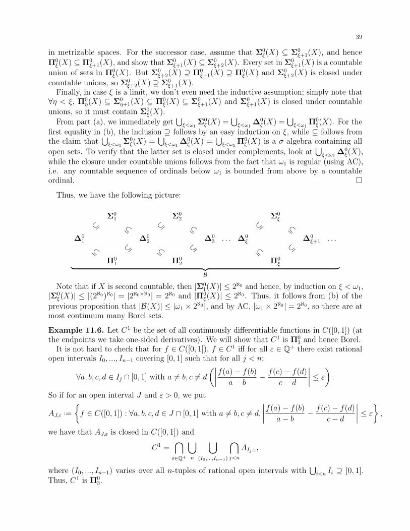
39

in metrizable spaces. For the successor case, assume that Σ0ξ(X) ⊆ Σ0

ξ+1(X), and hence

Π0ξ(X) ⊆ Π0

ξ+1(X), and show that Σ0ξ+1(X) ⊆ Σ0

ξ+2(X). Every set in Σ0ξ+1(X) is a countable

union of sets in Π0ξ(X). But Σ0

ξ+2(X) ⊇ Π0ξ+1(X) ⊇ Π0

ξ(X) and Σ0ξ+2(X) is closed under

countable unions, so Σ0ξ+2(X) ⊇ Σ0

ξ+1(X).Finally, in case ξ is a limit, we don’t even need the inductive assumption; simply note that∀η < ξ, Π0

η(X) ⊆ Σ0η+1(X) ⊆ Π0

ξ(X) ⊆ Σ0ξ+1(X) and Σ0

ξ+1(X) is closed under countable

unions, so it must contain Σ0ξ(X).

From part (a), we immediately get⋃ξ<ω1

Σ0ξ(X) =

⋃ξ<ω1

∆0ξ(X) =

⋃ξ<ω1

Π0ξ(X). For the

first equality in (b), the inclusion ⊇ follows by an easy induction on ξ, while ⊆ follows fromthe claim that

⋃ξ<ω1

Σ0ξ(X) =

⋃ξ<ω1

∆0ξ(X) =

⋃ξ<ω1

Π0ξ(X) is a σ-algebra containing all

open sets. To verify that the latter set is closed under complements, look at⋃ξ<ω1

∆0ξ(X),

while the closure under countable unions follows from the fact that ω1 is regular (using AC),i.e. any countable sequence of ordinals below ω1 is bounded from above by a countableordinal. �

Thus, we have the following picture:

Σ01 Σ0

2 Σ0ξ

⊆ ⊆ ⊆ ⊆ ⊆ ⊆∆0

1 ∆02 ∆0

3 . . . ∆0ξ ∆0

ξ+1 . . .

⊆ ⊆ ⊆ ⊆ ⊆ ⊆Π0

1 Π02 Π0

ξ︸ ︷︷ ︸B

Note that if X is second countable, then |Σ01(X)| ≤ 2ℵ0 and hence, by induction on ξ < ω1,

|Σ0ξ(X)| ≤ |(2ℵ0)ℵ0| = |2ℵ0×ℵ0| = 2ℵ0 and |Π0

ξ(X)| ≤ 2ℵ0 . Thus, it follows from (b) of the

previous proposition that |B(X)| ≤ |ω1 × 2ℵ0|, and by AC, |ω1 × 2ℵ0| = 2ℵ0 , so there are atmost continuum many Borel sets.

Example 11.6. Let C1 be the set of all continuously differentiable functions in C([0, 1]) (atthe endpoints we take one-sided derivatives). We will show that C1 is Π0

3 and hence Borel.It is not hard to check that for f ∈ C([0, 1]), f ∈ C1 iff for all ε ∈ Q+ there exist rational

open intervals I0, ..., In−1 covering [0, 1] such that for all j < n:

∀a, b, c, d ∈ Ij ∩ [0, 1] with a 6= b, c 6= d

(∣∣∣∣f(a)− f(b)

a− b− f(c)− f(d)

c− d

∣∣∣∣ ≤ ε

).

So if for an open interval J and ε > 0, we put

AJ,ε ..=

{f ∈ C([0, 1]) : ∀a, b, c, d ∈ J ∩ [0, 1] with a 6= b, c 6= d,

∣∣∣∣f(a)− f(b)

a− b− f(c)− f(d)

c− d

∣∣∣∣ ≤ ε

},

we have that AJ,ε is closed in C([0, 1]) and

C1 =⋂ε∈Q+

⋃n

⋃(I0,...,In−1)

⋂j<n

AIj ,ε,

where (I0, ..., In−1) varies over all n-tuples of rational open intervals with⋃i<n Ii ⊇ [0, 1].

Thus, C1 is Π03.

40

11.C. The classes Σ0ξ and Π0

ξ. Let B, Σ0ξ ,Π

0ξ ,∆

0ξ denote the classes of the corresponding

types of sets in metrizable spaces, for example Σ0ξ is the union of Σ0

ξ(X), where X variesover all metrizable spaces.

Proposition 11.7. For each ξ ≥ 1, the classes Σ0ξ ,Π

0ξ and ∆0

ξ are closed under continuouspreimages, i.e. if X, Y are Polish spaces, f : X → Y is continuous and A ⊆ Y is in one ofthese classes, then f−1(A) is also in the same class.

Proof. Easy induction on ξ. �

Let Γ be a class of sets in various spaces (such as Σ0ξ ,Π

0ξ , ∆0

ξ , B, etc.). We denote by

Γ(X) the collection of subsets of X that are in Γ. We also denote by Γ the dual class ofΓ, i.e. Γ(X) =∼ Γ(X), and we let ∆ denote its ambiguous part: ∆(X) = Γ(X) ∩ Γ(X).Furthermore, for any Polish space Y put

∃Y Γ = {proj1(A) : X is Polish, A ∈ Γ(X × Y )} ,∀Y Γ =∼ ∃Y Γ.

With this notation, we have the following:

Proposition 11.8. For all 1 6 ξ < ω1, Σ0ξ+1 = ∃NΠ0

ξ. Thus also Π0ξ+1 = ∀NΣ0

ξ.

Proof. Follows from the fact that the operation ∃N is the same as taking the union of thefibers. �

Thus,⋃

1≤n<ω Σ0ξ are all the sets that can be obtained from open sets using operations ∼,

∃N (and also the binary operation ∪). These set-theoretic operations obviously correspond tothe logical operations ¬, ∃, and ∨, where ∃ varies over N (arithmetical definability). Thesuperscript 0 in the notation Σ0

n,Π0n corresponds to the order of quantification: it is 0 in our

case as the quantification ∃N is done over N. We will later define classes Σ1n,Π

1n, where the

quantification is done over N = NN, i.e. functions from N to N. One could also define theclasses Σ2

n,Π2n using quantification over NN , i.e. functions from N to N, and so on.

11.D. Universal sets for Σ0ξ and Π0

ξ. The classes Σ0ξ ,Π

0ξ and ∆0

ξ provide for each Polishspace X a hierarchy for B(X) of at most ω1 levels. We will next show that this is indeed aproper hierarchy, i.e., all these classes are distinct, when X is uncountable. We will use theusual diagonalization technique due to Cantor:

Lemma 11.9 (Diagonalization). For a set X and R ⊆ X2, put AntiDiag(R) = {x ∈ X : ¬R(x, x)}.Then AntiDiag(R) 6= Rx for any x ∈ X.

Proof. Assume for contradiction that AntiDiag(R) = Rx, for some x ∈ X. Then we get acontradiction because

¬R(x, x) ⇐⇒ x ∈ AntiDiag(R) ⇐⇒ x ∈ Rx ⇐⇒ R(x, x). �

Thus, we first need to construct, for each ξ, a set that parameterizes Σ0ξ . The following

definition makes this precise:

Definition 11.10. Let Γ be a class of sets in topological spaces (such as Σ0ξ ,Π

0ξ , ∆0

ξ , B,etc.) and let X, Y be topological spaces. We say that a set U ⊆ Y ×X parameterizes Γ(X) if

{Uy : y ∈ Y } = Γ(X).

If, moreover, U itself is in Γ (i.e. U ∈ Γ(Y ×X)), we say that U is Y -universal for Γ(X).

41

Theorem 11.11. Let X be a separable metrizable space. Then for each ξ ≥ 1, there is aC-universal set for Σ0

ξ(X), and similarly for Π0ξ(X).

Proof. We prove by induction on ξ. Let (Vn)n∈N be an open basis for X. Because everyΣ0

1(=open) set is a union of some subsequence of these Vn, we define U ⊆ C ×X as follows:for y ∈ C, put

Uy ..=⋃

n,y(n)=1

Vn.

It is clear U parameterizes Σ01(X). Moreover, U is open because for (y, x) ∈ C ×X,

(y, x) ∈ U ⇐⇒ x ∈⋃

n,y(n)=1

Vn ⇐⇒ ∃n ∈ N (y(n) = 1 ∧ x ∈ Vn).

Thus indeed, U is C-universal for Σ01.

Note next that if U ⊆ C ×X is C-universal for Γ(X), then U c is C-universal for the dualclass Γ(X). In particular, if there is a C-universal set for Σ0

ξ(X), there is also one for Π0ξ(X).

Assume now that we have already defined C-universal sets V η for Π0η for all η < ξ.

Let ηn < ξ, n ∈ N, be such that ηn ≤ ηn+1 and sup {ηn + 1 : n ∈ N} = ξ. Because C ishomeomorphic to CN, it is enough to construct a CN-universal set for Σ0

ξ . Just like for the

open sets, define U ⊆ CN ×X as follows: for y ∈ CN, put

Uy ..=⋃n

V ηny(n).

By definition, U parameterizes Σ0ξ(X). To see why U itself is in Σ0

ξ , note that for (y, x) ∈CN ×X,

(y, x) ∈ U ⇐⇒ x ∈⋃n

V ηny(n) ⇐⇒ ∃n ∈ N V ηn(y(n), x).

The latter condition defines a set in Σ0ξ(X) because V ηn is in Σ0

ξ(C×X), the projection function

y 7→ y(n) is continuous for each n ∈ N, and Σ0ξ is closed under continuous preimages. �

Lemma 11.12 (Relativization to subsets). Let X be a topological space, Y ⊆ X, and let ξbe an ordinal with 1 ≤ ξ < ω1.

(a) If Γ is one of Σ0ξ ,Π

0ξ ,B, then Γ(Y ) = Γ(X)|Y ..= {A ∩ Y : A ∈ Γ(X)}.

(b) We also always have ∆0ξ(Y ) ⊇∆0

ξ(X)|Y . If moreover, Y ∈∆0ξ(X), then we also have

∆0ξ(Y ) ⊆∆0

ξ(X)|Y . However, the last inclusion is in general false for arbitrary Y .

Proof. Left as an exercise. �

Corollary 11.13. Let X be separable metrizable and Y be uncountable Polish. For any1 ≤ ξ < ω1, there is a Y -universal set for Σ0

ξ(X), and similarly for Π0ξ.

Proof. The existence of a Y -universal set for Σ0ξ(X) follows from that for Π0

ξ(X), so it is

enough to construct a Y -universal set for Π0ξ(X).

By the perfect set property for Polish spaces, there is a homeomorphic copy C ⊆ Y of theCantor space. By the above theorem, there is a C-universal set Uξ ∈ Π0

ξ(C×X) for Π0ξ(X); in

particular, U parameterizes Π0ξ(X). By the previous lemma, Π0

ξ(C ×X) = Π0ξ(Y ×X)|C×X ,

and since C ×X is closed in Y ×X (i.e. is in Π01(Y ×X)) and Π0

ξ(Y ×X) is closed under

finite (in fact, countable) intersections, Π0ξ(Y ×X)|C×X ⊆ Π0

ξ(Y ×X), so Uξ is still Π0ξ as a

42

subset of Y ×X, i.e. Uξ ∈ Π0ξ(Y ×X). (This wouldn’t be true for Σ0

1 and that’s why we chose

to construct a universal set for Π0ξ instead of Σ0

ξ .) Thus, Uξ is Y -universal for Π0ξ(X). �

Corollary 11.14. For every uncountable Polish space X and every 1 ≤ ξ < ω1, Σ0ξ(X) 6=

Π0ξ(X). In particular, ∆0

ξ(X) ( Σ0ξ(X) ( ∆0

ξ+1(X), and the same holds for Π0ξ.

Proof. Let U ⊆ X ×X be an X-universal set for Σ0ξ(X) and take A = AntiDiag(U). Since

A = δ−1(U c), where δ : X → X2 by x 7→ (x, x), A ∈ Π0ξ(X). However, by the Diagonalization

lemma, A 6= Ux for any x ∈ X, and thus A /∈ Σ0ξ(X). �

11.E. Turning Borel sets into clopen sets. The following theorem is truly one of themost useful facts about Borel sets. Recall that a Polish space X is formally a set X with atopology T on it (i.e. the collection of the open sets), so it is really a pair (X, T ). We denotethe Borel subsets of X by B(X, T ) or just B(T ), when we want to emphasize the topologywith respect to which the Borel sets are taken.

Theorem 11.15. Let (X, T ) be a Polish space. For any Borel set A ⊆ X, there is a finerPolish topology TA ⊇ T with respect to which A is clopen, yet B(TA) = B(T ).

We will prove this theorem after proving the following useful lemmas.

Lemma 11.16. Let (X, T ) be a Polish space. For any closed set F ⊆ X, the topology TFgenerated by T ∪ {F} is Polish. Moreover, F is clopen in TF and B(TF ) = B(T ).

Proof. The assertions in the second sentence of the statement are obvious. To see that TF isPolish, note that (X, TF ) is a direct sum of the topological spaces (F, T |F ) and (F c, T |F c),where T |F and T |F c are the relative topologies on F and F c as subspaces of (X, T ). Butthen (X, TF ) is Polish being a direct sum of two Polish spaces. �

Lemma 11.17. Let (X, T ) be a Polish space and let {Tn}n∈N be a sequence of Polishtopologies on X with T ⊆ Tn, for all n ∈ N. Then the topology T∞ generated by

⋃n Tn is

Polish. Moreover, if Tn ⊆ B(T ), for all n ∈ N, then B(T∞) = B(T ). (We will actually seelater that B(T∞) = B(T ) is already implied by ∀n ∈ N(T ⊆ Tn)).

Proof. 15 Let (Xn, Tn) be the topological space with the underlying set Xn = X and topologyTn. Then the product space Y ..=

∏n(Xn, Tn) is Polish, and we let δ : (X, T∞)→ Y be the

diagonal map: x 7→ (x, x, ...). By definition, δ is a continuous bijection from (X, T∞) to δ(X)because each coordinate function projn ◦δ : (X, T∞)→ (X, Tn) is continuous.

Claim. If a sequence(δ(xm)

)m∈N converges in Y , then (xm)m∈N converges in (X, T∞).

Proof of Claim. By the definition of product topology, for each n ∈ N, the projectionsprojn

(δ(xm)

)converge in Tn, as m→∞, to some yn ∈ Xn = X. But projn

(δ(xm)

)= xm,

so (xm)m∈N converges to yn in Tn, and hence also in T . Because T is Hausdorff, these ynmust all be equal and we denote the common value by y. Thus, (xm)m∈N converges to y inTn for all n ∈ N, and hence also in T∞. �

This claim implies that δ(X) is closed in Y and δ−1 is continuous, so δ is a homeomorphismbetween (X, T∞) and a closed subset of Y , and hence, (X, T∞) is Polish. �

15Thanks to Anton Bernshteyn for suggesting the exposition of this proof using sequences as opposed toopen sets.

43

Proof of Theorem 11.15. Let S be the collection of all sets A ⊆ X for which there exists aPolish topology TA ⊇ T ∪ {A} with B(TA) = B(T ). It is clear that S contains all of theopen sets, and by the last two lemmas, it also contains all of the closed sets and is closedunder countable unions. Thus, S contains all the Borel sets. �

We now give a couple of very useful applications.

Corollary 11.18. Borel subsets of Polish spaces have the PSP.

Proof. Let B be an uncountable Borel subset of a Polish space (X, T ). By the previoustheorem, there is a Polish topology T ′ ⊇ T in which B is clopen and hence (B, T ′|B) isPolish, where T ′|B denotes the relative topology on B with respect to T ′. Now by the PSPfor Polish spaces, there is an embedding f : C ↪→ (B, T ′|B). But then f is still continuous asa map from C into (B, T |B) as T |B has fewer open sets. Hence, because C is compact, f isstill automatically an embedding from C into (B, T |B). �

Corollary 11.19. Let (X, T ) be a Polish space, Y be a second countable space, and f : X →Y be a Borel function. There is a Polish topology Tf ⊇ T with B(Tf ) = B(T ) that makes fcontinuous.

Proof. Let {Vn}n∈N be a countable basis for Y and let Tn ⊇ T be a Polish topology on Xthat makes f−1(Vn) open and has the same Borel sets as T . By Lemma 11.17, the topologyT∞ generated by

⋃n Tn is Polish, and clearly, f : (X, T∞)→ Y is continuous. �

Corollary 11.20. Let (X, T ) be a Polish space and B ⊆ X be Borel. There is a closedsubset F ⊆ N and a continuous bijection f : F → B. In particular, if B 6= ∅, there is acontinuous surjection f : N � B.

Proof. Let T ′ ⊇ T be a Polish topology making B clopen. Hence (B, T ′|B) is Polish andand we apply Theorem 5.9. �

The proofs of the following two corollaries are left as exercises.

Corollary 11.21. Any Borel action Γ y (X, T ) of a countable group Γ on a Polish space(X, T ) has a continuous realization, i.e. there is a finer topology TΓ ⊇ T such that the actionΓ y (X, TΓ) is continuous.

Corollary 11.22. For any Polish (X, T ), there is a zero-dimensional Polish topology T0 ⊇ Twith B(T0) = B(T ).

12. Analytic sets

It is clear that the class of Borel sets is closed under continuous preimages, but is it closedunder continuous images?

Definition 12.1. A subset A of a Polish space X is called analytic if it is a continuous imageof a Borel subset of some Polish space; more precisely, if there is a Polish space Y , a Borelset B ⊆ Y and a continuous function f : Y → X such that f(B) = A.

Clearly, all Borel sets are analytic, but is the converse true? Historically, Lebesgue hada “proof” that continuous images of Borel sets are Borel, but several years later Souslinfound a mistake in Lebesgue’s proof; moreover, he constructed an example of a closed setwhose projection was not Borel. Hence continuous images of Borel sets were new kinds ofsets, which he and his advisor Luzin called analytic and systematically studied the propertiesthereof. This is often considered the birth of descriptive set theory.

44

12.A. Basic facts and closure properties. Before we exhibit an analytic set that is notBorel, we give the following equivalences to being analytic.

Proposition 12.2. Let X be Polish and ∅ 6= A ⊆ X. The following are equivalent:

(1) A is analytic.(2) There is Polish Y and continuous f : Y → X with A = f(Y ).(3) There is continuous f : N → X with A = f(N ).(4) There is closed F ⊆ X ×N with A = proj1(F ).(5) There is Polish Y and Borel B ⊆ X × Y with A = proj1(B).(6) There is Polish Y , Borel B ⊆ Y and Borel f : Y → X with A = f(B).

Proof. (4)⇒(5)⇒(1) are trivial, (1)⇒(2) is immediate from Theorem 11.15, (2)⇒(3) followsfrom Theorem 5.9, and (3)⇒(4) follows from the fact that graphs of continuous functions areclosed and f(Y ) = proj1(Graph(f)).

Finally, the implication (1)⇒(6) is trivial and the reverse implication follows from Corol-lary 11.19. Alternatively, one could deduce (6)⇒(5) from the fact that if f : Y → X andB ⊆ Y are Borel, then Graph(f |B) is Borel and f(B) = proj1(Graph(f |B)). �

Let Σ11 denote the class of all analytic subsets of Polish spaces, so for a Polish space X,

Σ11(X) is the set of all analytic subsets of X. Let Π1

1 =∼ Σ11 denote the dual class, and we

call the elements of Π11 co-analytic. By (4) of the above proposition, we have

Σ11 = ∃NB = ∃NΠ0

1,

and consequently,

Π11 = ∀NB = ∀NΣ0

1.

Furthermore, put ∆11 = Σ1

1 ∩Π11. It is clear that B ⊆∆1

1, and we will see later that they areactually equal. For now, we will just list some closure properties of Σ1

1:

Proposition 12.3. The class Σ11 is closed under

(i) continuous images and preimages;(ii) (in fact) Borel images and preimages;(iii) countable intersections and unions.

Proof. We only prove the closure under countable intersections and leave the rest as anexercise. Let An be analytic subsets of a Polish space X. By (4) of Proposition 12.2, thereare closed sets Cn ⊆ X ×N such that An = proj1(Cn). Let Y = X ×N N and consider theset C ⊆ Y defined by

(x, (yn)n∈N) ∈ C :⇔ ∀n ∈ N(x, yn) ∈ Cn.

Clearly, C is Borel (in fact it is closed) and⋂nAn = proj1(C). �

12.B. A universal set for Σ11. We now focus on showing that Σ1

1 6= Π11 and hence there

are analytic sets that are not Borel. As with the Borel hierarchy, we start with a universalanalytic set:

Theorem 12.4 (Souslin). For any uncountable Polish Y and Polish X, there is a Y -universalset U ⊆ Y ×X for Σ1

1(X). The same holds for Π11(X).

45

Proof. The idea is to use (4) of Proposition 12.2, so we start with a Y -universal set F ⊆Y × (X × N ) for Π0

1(X × N ), which exists by Corollary 11.13. Put U ..= proj1,2(F ) ..={(y, x) ∈ Y ×X : ∃z ∈ N (y, x, z) ∈ F} and note that U is analytic being a projection of aclosed set. We claim that U is universal for Σ1

1(X). Indeed, let A ⊆ X be analytic, so by(4) of Proposition 12.2, there is a closed set C ⊆ X ×N with A = proj1(C). Then there isy ∈ Y with Fy = C and hence A = proj1(C) = proj1(Fy) = (proj1,2(F ))y = Uy and we aredone. �

Corollary 12.5 (Souslin). For any uncountable Polish space X, Σ11(X) 6= Π1

1(X). Inparticular, B(X) ⊆∆1

1(X) 6= Σ11(X), and same for Π1

1(X).

Proof. Take an X-universal set U ⊆ X ×X for Σ11(X) and put

A ..= AntiDiag(U) = {x ∈ X : (x, x) /∈ U} .Let δ : X → X ×X by x 7→ (x, x) and note that it is continuous. Because A = δ−1(U c) andU c is co-analytic, A is also co-analytic. However, it is not analytic since otherwise A wouldhave to be equal to a fiber Ux of U , for some x ∈ X, contradicting the diagonalization lemma.

In particular, A is not Borel, so Ac is analytic but not Borel. �

12.C. Analytic separation and Borel = ∆11.

Theorem 12.6 (Luzin). Let X be a Polish space and let A,B ⊆ X be disjoint analytic sets.There is a Borel set D ⊆ X that separates A and B, i.e. D ⊇ A and Dc ⊇ B.

Proof. Call disjoint sets P,Q ⊆ X Borel-separable if there is a Borel set R ⊆ X with R ⊇ Pand R ∩Q = ∅. Note that the collection of sets that are Borel-separable from a given set Qforms a σ-ideal: indeed, if P =

⋃n Pn and each Pn is separable from Q by Rn, then the set⋃

nRn separates P from Q. Thus we have:

Claim. If P =⋃n Pn and Q =

⋃mQm, and Pn, Qm are Borel-separable for any n,m ∈ N,

then P,Q are Borel-separable.

Proof of Claim. First fix n and note that Pn is separable from Q since it is separable fromeach Qm. But then Q is separable from P . �

An obvious example of disjoint sets that are Borel-separable are distinct singletons {x} , {y}(because X is Hausdorff). Iterating the above claim, we will show that if A,B are not Borel-separable, then it should boil down to two singletons not being Borel-separable, which wouldbe a contradiction.

Let f : N → A and g : N → B be continuous surjections, which exist by (3) ofProposition 12.2. Put As ..= f(Ns) and Bs

..= g(Ns) for each s ∈ N<N. Using the claim, wecan follow the non-Borel-separable branch of N<N and recursively define x, y ∈ N such thatfor every n ∈ N, Ax|n and By|n are not Borel-separable. Put a ..= f(x) and b ..= g(y). BecauseA and B are disjoint, a 6= b, so there are disjoint open neighborhoods U 3 a and V 3 b. Bythe continuity of f and g, there is n such that Ax|n = f(Nx|n) ⊆ U and By|n = g(Ny|n) ⊆ V .So Ax|n and By|n are Borel-separable, contradicting the choice of x and y. �

Corollary 12.7 (Souslin). Let X be Polish and A ⊆ X. If A and Ac are both analytic, thenA is Borel. In other words, B(X) = ∆1

1(X).

Proof. Take a Borel set B separating A and Ac and note that B has to be equal to A. �

Corollary 12.8. Let X, Y be Polish and f : X → Y . The following are equivalent:

46

(1) f is Borel;(2) The graph of f is Borel;(3) The graph of f is analytic.

Proof. (1)⇒(2): Fix a countable basis {Vn}n∈N for Y and note that for (x, y) ∈ X × Y , wehave

f(x) = y ⇐⇒ ∀n(y ∈ Vn → x ∈ f−1(Vn)).

ThusGraph(f) =

⋂n

(proj−1

2 (V cn ) ∪ proj−1

1 (f−1(Vn))),

and hence is Borel.(3)⇒(1): Assume (3) and let U ⊆ Y be open; we need to show that f−1(U) is Borel. But forx ∈ X, we have

x ∈ f−1(U) ⇐⇒ ∃y ∈ Y (f(x) = y and y ∈ U)

⇐⇒ ∀y ∈ Y (f(x) = y → y ∈ U),

so f−1(U) is both analytic and co-analytic, and hence is Borel by Souslin’s theorem. �

Corollary 12.9. Let X be Polish and let {An}n∈N be a disjoint family of analytic subsets ofX. Then there is a disjoint family {Bn}n∈N of Borel sets with Bn ⊇ An.

12.D. Souslin operation A. In this subsection, we will define an important operation onschemes of sets and we will give yet another characterization of analytic sets in terms of thisoperation.

For a set X and a pruned tree T ⊆ N<N, we refer to a sequence of subsets (Ps)s∈T of X asa Souslin scheme on X. Call this scheme monotone if

(i) Pt ⊆ Ps for all t ⊇ s, s, t ∈ T ,

and call it proper 16 if it is monotone and also

(ii) Psai ∩ Psaj = ∅, for all s ∈ T , i 6= j, i, j ∈ T (s).

Definition 12.10. We define the Souslin operation A applied to an arbitrary Souslin scheme(Ps)s∈T as follows:

A(Ps)s∈T ..=⋃y∈[T ]

⋂n∈N

Py|n .

Note that by taking some of the sets to be empty, we can always assume that T = N<N.Also note that we don’t require (Ps)s∈T to be proper (not even monotone). In fact, thefollowing lemma shows that when it is proper, this operation trivializes in the sense that theuncountable union is replaced by a countable union:

Lemma 12.11. If (Ps)s∈T is a proper Souslin scheme, then A(Ps)s∈T =⋂n∈N

⋃s∈T,|s|=n

Ps.

Proof. The inclusion ⊆ follows easily by taking s = y|n for each n. For ⊇, take

x ∈⋂n∈N

⋃s∈T,|s|=n

Ps,

16This generalizes our earlier definition of a Luzin scheme.

47

so for each n, there is sn ∈ T of length n such that x ∈ Psn . The sequence (sn)n must becoherent (i.e. increasing) because otherwise, if n < m and sn * sm, then by monotonicity,x ∈ Pt with t = sm|n, so x ∈ Pt ∩ Psn 6= ∅, contradicting properness. �

For a class Γ of subsets in topological spaces, let AΓ denote the class of all sets of theform A(Ps)s∈N<N , where each Ps ∈ Γ(X), for a fixed topological space X.

The following shows that the operation A can be implemented via projection.

Lemma 12.12. For a Souslin scheme (Ps)s∈N<N on a set X, A(Ps)s∈N<N = proj1(P ), whereP ⊆ X ×N is defined as follows: for (x, y) ∈ X ×N ,

(x, y) ∈ P ..⇐⇒ ∀n ∈ N ∃s ∈ N<N y|n = s ∧ x ∈ Ps⇐⇒ ∀n ∈ N ∀s ∈ N<N y|n 6= s ∨ x ∈ Ps.

In particular, if Γ is a class of subsets in topological spaces that contains clopen sets and isclosed under finite unions and countable intersections, then AΓ ⊆ ∃NΓ.

Proof. Straightforward, left as an exercise. �

The next lemma shows that the converse also holds for Γ = Σ11.

Lemma 12.13. Let T ⊆ N<N be a pruned tree, X a Polish space and f : [T ]→ X continuous.Then Ps ..= f([Ts]) is analytic for each s ∈ T , and the Souslin scheme (Ps)s∈T satisfies thefollowing:

(i) for each s ∈ T , Ps 6= ∅;(ii) for each s ∈ T , Ps =

⋃i∈T (s) Psai (in particular, it is monotone);

(iii) for each y ∈ [T ] and U ⊆ X open, if Py ..=⋂n Py|n ⊆ U , then Py|n ⊆ U for some n ∈ N;

(iv) it is of vanishing diameter, i.e. for all y ∈ [T ], diam(Py|n)→ 0 as n→∞.

Moreover, f([T ]) = A(Ps)s∈T = A(Ps)s∈T .

Proof. The properties (i)-(ii) and the equality f([T ]) = A(Ps)s∈T are immediate from thedefinition of (Ps)s∈T , and (iii)-(iv) follow from the continuity of f . The equality A(Ps)s∈T =A(Ps)s∈T also follows from the continuity of f as follows: it is enough to show that for fixedy ∈ [T ],

⋂n Py|n ⊆

⋂n Py|n , so take x ∈

⋂n Py|n , and we claim that f(y) = x. Otherwise,

there are disjoint open sets U, V ⊆ X such that U 3 f(y) and V 3 x, so x /∈ U . But by (iii),there is n ∈ N such that Py|n ⊆ U , so x /∈ Py|n , a contradiction. �

Proposition 12.14 (Characterization of analytic via operation A). Let X be Polish and∅ 6= A ⊆ X. The following are equivalent:

(1) A is analytic.(2) A = A(Fs)s∈N<N, where each Fs is nonempty closed, and the Souslin scheme (Fs)s∈N<N

is monotone and of vanishing diameter (for any compatible metric on X).(3) A = A(Ps)s∈N<N, where each Ps is analytic.

In particular, Σ11 = AΣ1

1 = AΠ01.

Proof. (1)⇒(2): Suppose A is analytic, so, by Proposition 12.2, A = f(N ) for some continuousfunction f : N → X. Putting Ps = f(Ns), (2) follows from 12.13 by taking Fs = Ps.(2)⇒(3): Trivial.(3)⇒(1): Follows immediately from Lemma 12.12. �

48

13. More on Borel sets

13.A. Closure under small-to-one images. In general, images of Borel sets under Borelfunctions are analytic and may not be Borel. However, the situation may be different if thepreimage of every point is “small”. In this subsection, we will state and prove some resultswith various notions of “small”, starting from the cases where the domain space itself if“small”.

Below we use the terms σ-compact or Kσ for subsets of topological spaces that are countableunions of compact sets.

Proposition 13.1.

(a) Continuous functions map compact sets to compact sets.(b) Continuous functions map Kσ sets to Kσ sets.(c) Tube lemma. For topological spaces X, Y with Y compact, proj1 maps closed subsets

of X × Y to closed subsets of X.

Proof. (a) is just by unraveling the definitions and it immediately implies (b). For (c), letF ⊆ X × Y be closed, x /∈ proj1(F ) and consider the open cover (Vy)y∈Y of Y where Vy 3 yis open and is such that for some nonempty open neighborhood Uy ⊆ X of x, Uy × Vy isdisjoint from F . �

Examples 13.2.

(a) proj1 : R× R→ R does not, in general, map closed sets to closed sets: e.g., take F tobe the graph of 1/x with domain (0, 1]; then F is closed, but its projection is (0, 1].

(b) However, because R is σ-compact (hence Kσ = Fσ) and Hausdorff (hence compact setsare closed), it follows from (b) of Proposition 13.1 that proj1 : R×R→ R maps Fσ sets(in particular, closed sets) to Fσ sets.

The following is one of the most used results in descriptive set theory.

Theorem 13.3 (Luzin–Souslin). Let X, Y be Polish spaces and f : Y → X be Borel. IfA ⊆ Y is Borel and f |A is injective, then f(A) is Borel.

Proof. By Corollary 11.19 (or by replacing Y with Y ×X, A with Graph(f |A), and f withproj2), we may assume that f is continuous. Moreover, by Corollary 11.20, we may assumethat Y = N and A ⊆ N is closed. Thus, A = [T ] for some pruned tree T ⊆ N<N. For eachs ∈ T , put Ps = f([Ts]) and hence each Ps is analytic and, by Lemma 12.13, we have

f([T ]) = A(Ps)s∈T = A(Ps)s∈T .

Note that by injectivity of f |[T ], the scheme (Ps)s∈T is proper, so

f([T ]) = A(Ps)s∈T =⋂n∈N

⋃s∈T,|s|=n

Ps,

but this still doesn’t imply that f([T ]) is Borel since each Ps may not be Borel. On the otherhand, with (Ps)s∈T it is the opposite: each Ps is Borel, but the scheme (although monotone)may not be proper. We fix this by approximating Ps from outside by a Borel set Bs whilestaying within Ps. This is done using iterative applications of the analytic separation theoremas follows: for each n, recursively apply Corollary 12.9 to the collection {Ps : s ∈ T, |s| = n}to get pairwise disjoint sequence (Bs)s∈T of Borel sets with Ps ⊆ Bs. By taking intersections,

49

we may assume that Bs ⊆ Ps, as well as Bs ⊆ Bt for every t ⊆ s. Thus, (Bs)s∈T is a properSouslin scheme, as desired.

Because Ps ⊆ Bs ⊆ Ps, we have

A(Ps)s∈T ⊆ A(Bs)s∈T ⊆ A(Ps)s∈T ,

so all these inclusions are actually equalities. Finally, because (Bs)s∈T is proper, we have

f([T ]) = A(Ps)s∈T = A(Bs)s∈T =⋂n∈N

⋃s∈T,|s|=n

Bs,

and hence f([T ]) is Borel. �

Corollary 13.4. Let X, Y be Polish and f : X → Y be Borel. If f is injective, then it is aBorel embedding, i.e. f maps Borel sets to Borel sets.

The Luzin–Souslin theorem together with Corollary 11.20 gives the following characteriza-tion of Borel sets:

Corollary 13.5. A subset B of a Polish space X is Borel iff it is an injective continuousimage of a closed subset of N .

This shows the contrast between Borel and analytic as the latter sets are just continuousimages of closed subsets of N .

Now, how big can the “small” be so that the Borel sets are still closed under “small”-to-oneimages? It turns out that for small being σ-compact, this is still true and this is a deeptheorem of Arsenin and Kunugui [Kec95, 18.18]. Here we will only state a very importantspecial case of this, which will be enough for our purposes.

For topological spaces X, Y , call a set A ⊆ X × Y a Borel graph if A is Borel and for everyx ∈ X, the fiber Ax := {y ∈ Y : (x, y) ∈ A} has at most one element.

Theorem 13.6 (Luzin–Novikov). Let X, Y be Polish spaces and B ⊆ X × Y be a Borel setall of whose X-fibers are countable, i.e. for every x ∈ X, Bx is countable. Then B can bepartitioned into countably many disjoint Borel graphs B =

⊔nBn.

In Subsection 22.B, we will deduce the last theorem from another big theorem about graphcolorings.

Corollary 13.7. The class of Borel subsets of Polish spaces is closed under countable-to-oneBorel images.

Proof. Let Z,X be Polish spaces, f : Z → X be a countable-to-one Borel function, B ⊆ Z aBorel set, and we show that f(B) is Borel. By replacing B with Graph(f |B), we may assumethat Z = X × Y , for some Polish space Y , and f = proj1. By the Luzin–Novikov theorem,B =

⊔nBn, where each Bn is a Borel graph. For each n, f(Bn) is Borel by Theorem 13.3,

and thus, so is f(B) =⋃n f(Bn). �

The next corollary says, in particular, that given a Borel set B ⊆ X × Y with countableX-fibers, for each x ∈ proj1(B), we can choose in a Borel way (“uniformly”) a witness y ∈ Ywith (x, y) ∈ B.

Corollary 13.8 (Countable uniformization). For Polish spaces Z,X, any countable-to-oneBorel function f : Z → X admits a Borel right inverse g : f(Z)→ Z.

50

Proof. Just like in the proof of Corollary 13.7, we may assume that Z = X×Y and f = proj1.By the Luzin–Novikov theorem, B =

⊔nBn, where each Bn is a Borel graph. Define

k : X → N by x 7→ the least n ∈ N with x ∈ proj1(Bn), and finally define g : X → X × Y byx 7→ (x, y), where y ∈ Y is the unique element with (x, y) ∈ Bk(x). It is straightforward tocheck that the function k, and hence also g, is Borel. �

13.B. The Borel isomorphism theorem. Using that the Borel sets are closed under one-to-one Borel images, we show in this subsection that any two uncountable Polish spaces areBorel isomorphic.

Corollary 13.9 (The Borel Schroder–Bernstein theorem). Let X, Y be Polish and f : X ↪→ Y ,g : Y ↪→ X be Borel injections. Then X and Y are Borel isomorphic.

Proof. Run the same proof as for the regular Schroder–Bernstein theorem and note that allthe sets involved are images of Borel sets under f or g, and hence are themselves Borel. Thus,the resulting bijection is a Borel isomorphism. �

The following theorem shows how robust the framework of Polish spaces is when studyingBorel sets and beyond.

Theorem 13.10 (The Borel Isomorphism Theorem). Any two Polish spaces of the samecardinality are Borel isomorphic. In particular, any two uncountable Polish spaces are Borelisomorphic.

Proof. The statement for countable Polish spaces is obvious since their Borel σ-algebrais all of their powerset. For uncountable Polish space, it is enough to show that if X isuncountable, then it is Borel isomorphic to C. By the Borel Schroder–Bernstein, it is enoughto show that there are Borel injections C ↪→ X and X ↪→ N since N embeds into C. By theCantor–Bendixson theorem and the perfect set theorem, there is a continuous embedding ofC into X. It remains to show that X ↪→ N and we give two ways to see this.Way 1: By Theorem 5.9, there is a closed set F ⊆ N and a continuous bijection f : F → X.But then, by Theorem 13.3, f−1 : X → N is a Borel embedding.Way 2: By Corollary 11.22, we may assume that X is zero-dimensional. But then X ishomeomorphic to a closed subset of N , by Theorem 5.8. �

13.C. Standard Borel spaces. As the Borel Isomorphism Theorem shows, it really doesnot matter which Polish space to consider when working in the Borel context. The followingdefinition makes abstracting from the topology but keeping the Borel structure precise.

Definition 13.11. A measurable space (X,S) is called a standard Borel space if there is aPolish topology T on X such that B(T ) = S . In this case, we call T a compatible Polishtopology and refer to the sets in S as Borel sets. Similarly, we call a subset A ⊆ X analytic(resp. co-analytic) if for some (equivalently any) compatible Polish topology T , A is analytic(resp. co-analytic) as a subset of (X, T ).

In the definition above, the notion of an analytic set is well-defined, i.e. it does notdepend on which compatible Polish topology one picks; indeed, if T , T ′ are compatible Polishtopologies on X, then the identity map from (X, T ) to (X, T ′) is a Borel isomorphism, andhence A is analytic in (X, T ) iff it is analytic in (X, T ′).Examples 13.12.

51

(a) An obvious example of a standard Borel space is a Polish space with its Borel σ-algebra:(X,B(X)).

(b) A less immediate example is a Borel subset A of a Polish space X with the relative Borelσ-algebra: (A,B(X)|A), where B(X)|A = {B ∩ A : B ∈ B(X)} = {B ∈ B(X) : B ⊆ A}.This is because there is a Polish topology on X making A clopen and hence Polish inthe relative topology.

13.D. The Effros Borel space. We now consider an interesting and important example ofa standard Borel space. For a topological space X, let F (X) denote the collection of theclosed subsets of X. We endow F (X) with the σ-algebra E generated by the sets of the form

[U ]F(X)..= {F ∈ F (X) : F ∩ U 6= ∅} ,

for U open in X. If X has a countable basis {Un}n∈N, it is of course enough to consider U inthat basis. The measurable space (F (X), E) is called the Effros Borel space of X.

Theorem 13.13. For any Polish space X, the Effros Borel space of X is standard.

Proof. Let (Un)n∈N be a countable basis for X and consider the map c : F (X)→ C by F 7→the characteristic function of {n ∈ N : F ∩ Un 6= ∅}. It is clear that c is measurable sincethe preimage of a pre-basic open set {x ∈ C : x(n) = i}, for i ∈ {0, 1}, is [Un]F(X) or itscomplement, depending on whether i = 1 or 0. It is also clear that c is injective and, lettingY ..= c(F (X)),

c([Un]F(X)

)= {x ∈ C : x(n) = 1} ∩ Y,

so c−1 : Y → F (X) is also measurable. This makes c an isomorphism between measurablespaces (F (X), E) and (Y,B(C)|Y ). Hence, if Y is Borel, then these measurable spaces arestandard Borel.

We in fact show that Y is a Gδ subset of C. Indeed, fix a complete compatible metric onX. Then one can verify (left as a homework exercise) that for x ∈ C,

x ∈ Y ⇐⇒ ∀Un ⊆ Um[x(n) = 1→ x(m) = 1]

and

∀Un∀ε ∈ Q+[x(n) = 1→ ∃Um ⊆ Un with diam(Um) < ε such that x(m) = 1)

].

Thus, Y is clearly Gδ. �

As the following example shows, the fact that the Effros space is standard Borel allowsconsidering spaces of seemingly third order objects, such as Polish spaces themselves, in thecontext of Polish spaces.

Example 13.14. Theorem 3.7 states that we can think of F (RN) as the space of all Polishspaces, and by Theorem 13.13, it is a standard Borel space. This allows us, for example, totalk about the homeomorphism of Polish spaces as an equivalence relation on F (RN).

Lastly, we will discuss the possibility of choosing a “canonical” point from every nonemptyclosed subset of a Polish space.

Definition 13.15. Let X be a Polish space. A function s : F (X)→ X is called a selectorif s(F ) ∈ F for every nonempty F ∈ F (X).

52

Intuitively, one can recognize when such a selector is canonical; for example, choosing theleftmost branch of TC for a given nonempty closed subset C ⊆ N . Another example is fora nonempty closed subset C ⊆ R, let M ∈ N be the least such that C ∩ [−M,M ] 6= ∅ andchoose the point c = min(C ∩ [−M,M ]) from C. For a general Polish space X, the Effrosstructure on F (X) makes the notion of canonical precise: simply require the selector functionto be Borel! The following shows that such a function always exists.

Theorem 13.16. For every Polish space X, the Effros Borel space F (X) admits a Borelselector.

Proof. Outlined in a homework exercise. �

13.E. Borel determinacy. We have already proven that Borel sets have the PSP and theyalso clearly have the BP because the collection of sets with BP forms a σ-algebra. Borel setsare also obviously measurable under any Borel measure. In this subsection, we discuss thedeterminacy of Borel sets, and we start with open/closed sets. For the rest of the section letA be a discrete set and let T ⊆ A<N be a pruned tree on which the games will be played (soT is a game with rules).

Theorem 13.17 (Gale–Stewart). Any open or closed subset D ⊆ [T ] is determined, i.e. thegame G(T,D) is determined.

Proof. Suppose D is open or closed, so the payoff set O for one of the players is open and forthe other one the payoff set C is closed (of course, {O,C} = {D,Dc}). We refer the formeras Player O and to the latter as Player C. Call a position p ∈ T winning for Player O if hehas a winning strategy starting from p. Clearly we have the following:

Claim. Let p ∈ T be not winning for Player O. If it is Player C’s turn to play, then there isa legal move a ∈ A that Player C can make so that the position paa ∈ T is still not winningfor Player O. If it is Player O’s turn to play, then no matter what legal a ∈ A he plays, thenew position paa ∈ T will still be not winning for Player O.

Now suppose Player O does not have a winning strategy; in other words, ∅ ∈ T is notwinning for Player O. We inductively construct a winning strategy for Player C as follows:assuming that the game is at position p ∈ T that is not winning for Player O and it is PlayerC’s turn to play, then Player C chooses an extension of p that is still not winning for PlayerO. If Player C plays according to this strategy, then the run of the game x ∈ [T ] is suchthat for every n ∈ N, x|n is not winning for Player O. Thus, x must be in the closed payoffset C since otherwise, if x ∈ O, then there would be n ∈ N with [Tx|n ] ⊆ O and hence x|nwould be winning for Player O, a contradiction. �

Although this theorem only proves determinacy for open/closed sets, we will use it inproving regularity properties of analytic sets. We can do this mainly because analytic setsare projections of closed subsets of X ×N , so we will somehow construct equivalent gameson these closed subsets and use their determinacy to conclude determinacy for the originalgames for analytic sets.

The following is one of the most important and grandiose results in descriptive set theory:

Theorem 13.18 (Borel Determinacy, Martin 1975). For any set A (possibly uncountable)and any tree T ⊆ A<N, all Borel sets B ⊆ [T ] are determined.

53

We won’t give the proof of this theorem here, but we will describe its general flow. Bydefinition, every Borel set in [T ] can be (transfinitely) “unraveled” up to clopen sets. Similarly,the main idea of the proof is to “unravel” every Borel game to a clopen game in such a waythat the determinacy of the latter (which we know holds) implies that of the former. Thefollowing makes this precise:

Definition 13.19. Let T ⊆ A<N be a tree. A covering of T is a triple (T , π, ϕ) where

(i) T is a pruned tree on some set A.

(ii) π : T → T is a length-preserving (i.e. |π(s)| = |s| for s ∈ T ) monotone map (think of

it as a projection). Thus, π gives rise to a continuous function π∗ : [T ]→ [T ]. We willabuse the notation and still write π for π∗.

(iii) ϕ maps strategies for Player I (resp. II) in T (i.e. certain pruned subtrees) to strategies

for Player I (resp. II) in T in such a way that for a strategy σ in T , ϕ(σ) restricted topositions of length ≤ n depends only on σ restricted to positions of length ≤ n.

(iv) If σ is a strategy in T , then ϕ([σ]) ⊇ [ϕ(σ)]. In other words, if a run x ∈ [T ] is played

according to ϕ(σ), then there is a run x ∈ [T ] played according to σ such that π(x) = x.

It should be clear from the definition that for D ⊆ [T ], the game G(T,D) can be simulatedby the game G(T , D), where D = π−1(D). More precisely, if σ is a winning strategy forPlayer I (resp. II) in G(T , D), then ϕ(σ) a winning strategy for the same player in G(T,D).

Definition 13.20. We say that a covering (T , π, ϕ) of T unravels D ⊆ [T ] if π−1(D) ⊆ [T ]is clopen.

Thus, if (T , π, ϕ) unravels D ⊆ [T ], then, by the Gale–Stewart theorem, G(T , π−1(D)) isdetermined, and hence so is G(T,D). So to prove Borel determinacy, it is enough to provethat for every Borel set D ⊆ [T ] there is a covering (T , π, ϕ) of T that unravels D. The proofis done by transfinite induction on the construction of Borel sets17. The hardest part (theheart of the proof) is the base case, i.e. showing that open sets can be unraveled. As forthe inductive step, first note that if D ⊆ [T ] can be unraveled, then the same covering alsounravels [T ] \ D. So we only need to show that if An are unraveled by (Tn, πn, ϕn), thenA =

⋃nAn can be unraveled as well. By taking an inverse limit (in some appropriate sense)

of the coverings18 (Tn, πn, ϕn), we get a covering that unravels all An simultaneously, so thepreimage of A is open and hence it can be unraveled further using the base of the induction.

14. Regularity properties of analytic sets

In this section we prove that analytic sets enjoy the PSP and the BP. The determinacy ofanalytic sets is already independent of ZFC (under some large cardinal hypothesis19).

We have already considered games that are associated to these properties, namely the∗-game G∗(D) and the ∗∗-game G∗∗(D), for D ⊆ X, where X is a perfect Polish space. Notethat either of these games is played on a certain countable pruned tree T of legal positions.In the case of the ∗-game, the moves of the players are from the set A = {0, 1} ∪W2, where

17For the induction to go through, one actually has to construct so-called k-coverings instead of coverings,but we will keep this technicality out of our exposition.

18One has to actually take a coherent sequence of coverings (Tn, πn, ϕn), which we assume exists byinduction.

19It is actually equivalent to the existence of sharps.

54

W is a weak basis for X, and in the case of the ∗∗-game A = W . Let g : [T ] → X be thefunction that associates an element x ∈ X with a given run a ∈ [T ] in either of these games:

for the ∗-game, {x} =⋂n U

(n)in

, and for the ∗∗-game, {x} =⋂n Un. In either game, it is clear

that this function is continuous. In particular, if D ⊆ X is closed (resp. Borel, analytic, etc),then so is g−1(D) ⊆ [T ]. Thus Σ1

1-determinacy automatically implies that analytic sets havethe PSP and the BP.

However, as mentioned above, Σ11-determinacy is independent from ZFC, so we can’t use

it to prove that all analytic sets have the PSP and the BP (in ZFC). Instead, based onthe fact that analytic subsets of X are projections of closed subsets of X ×N , we will usethe so-called unfolding technique to reduce the determinacy of the ∗- and the ∗∗-games foranalytic sets to that for closed sets, whose determinacy we already know (the Gale–Stewarttheorem).

14.A. The perfect set property. We start with defining the unfolded ∗-game. SupposeX is a perfect Polish space and let F ⊆ X ×N . The unfolded ∗-game G∗u(F ) for F is thefollowing:

I (U(0)0 , U

(0)1 ), y0 (U

(1)0 , U

(1)1 ), y1

· · ·II i0 i1

where Players I and II play as they do in the ∗-game, but additionally Player I plays yn ∈ Nis his nth move. If {x} =

⋂n U

(n)in

and y = (yn)n∈N, then Player I wins iff (x, y) ∈ F .

Theorem 14.1. Let X be a perfect Polish space, F ⊆ X ×N , and A = proj1(F ). Then

(a) Player I has a winning strategy in G∗u(F ) ⇒ A contains a Cantor set.(b) Player II has a winning strategy in G∗u(F ) ⇒ A is countable.

Proof. (a) If Player I has a winning strategy in G∗u(F ), then ignoring the y(n)-s, we get awinning strategy for Player I in the original game G∗(A), so A contains a Cantor set.(b) Assume Player II has a winning strategy σ in G∗u(F ). For each x ∈ A, we choose a witnessy ∈ N , so that (x, y) ∈ F . Call a position

p = (((U(0)0 , U

(0)1 ), y0, ), i0, ..., ((U

(n)0 , U

(n)1 ), yn), in)

good for (x, y) if it is played according to σ (i.e. p ∈ σ), y ⊇ (yi)i≤n and x ∈ Uin . For aposition p as above, and for b ∈ N, let Ap,b denote the set of x ∈ X such that p doesn’t havea good extension for (x, y), for any y ∈ N that extends (yi)i≤n

ab, i.e.

Ap,b ..= {x ∈ X : ∀ legal moves ((U(n+1)0 , U

(n+1)1 ), b), if in+1 is played by II according to σ

then x /∈ U (n+1)in+1

}.

As before, for every (x, y) ∈ F , there must exist a maximal good position p ∈ σ sinceotherwise (x, y) ∈ [σ], contradicting σ being a winning strategy for Player II. Thus, for suchp and b = y(n+ 1), x ∈ Ap,b, and hence

A ⊆⋃

p∈σ,b∈N

Ap,b.

55

To conclude that A is countable, it remains to note that each Ap,b can have at most oneelement; indeed, if x, z ∈ Ap,b and x 6= z, then by Hausdorffness, there is a legal move

((U(n+1)0 , U

(n+1)1 ), b) of Player I such that x ∈ U (n+1)

0 and z ∈ U (n+1)1 , so regardless of what

Player II’s response in+1 is, U(n+1)in+1

contains either x or z, contradicting x, z ∈ Ap,b. �

Corollary 14.2. Analytic subsets of Polish spaces have the PSP.

Proof. Let X be a Polish space and let A ⊆ X be analytic. By taking X = its perfectkernel, we may assume that X is perfect. Now let F ⊆ X × N be a closed set such thatA = proj1(F ). If g : [T ]→ X ×N is the function associating an element (x, y) ∈ X ×N toevery run of G∗u(F ), then g−1(F ) is closed and hence the game G∗u(F ) is determined (by theGale–Stewart theorem). Thus, by the previous theorem, A is either countable or contains aCantor set. �

We now give a completely different (probabilistic in spirit) proof of the PSP for analyticsets using the notion of Baire category in the hyperspace K(X) of compact sets, for a Polishspace X. Here we use that analytic sets are continuous images of Polish spaces, i.e. A ⊆ Y isanalytic if there is Polish X and continuous f : X → Y such that f(X) = A.

Theorem 14.3. Let X, Y be Polish spaces and f : X → Y be a continuous function suchthat A = f(X) is uncountable. Then there is a Cantor set C ⊆ X such that f |C is injective.In particular, f(C) is a Cantor set in A, and hence any analytic set has the PSP.

Proof. By restricting to the perfect kernel of X, we may assume without loss of generalitythat X is perfect. In particular, by Corollary 4.5, the set Kp(X) of all perfect compact setsis dense Gδ in K(X). Thus, to prove the theorem, it is enough to show that the set

Kf (X) = {K ∈ K(X) : f |K is injective}is a dense Gδ subset of K(X) since then Kp(X) ∩Kf (X) 6= ∅, and hence there is a compactperfect set K ∈ Kf (X), which of course contains a Cantor set, concluding the proof.

To ensure the density of Kf(X), we assume without loss of generality that for everynonempty open U ⊆ X, f(U) is uncountable. This can be achieved as follows: fix a countablebasis {Un}n∈N and subtract from X all the Un for which f(Un) is countable. By doing so,we have thrown away all open sets U for which f(U) is countable. The remaining set X ′ isnonempty since f(X ′) is still uncountable, and X ′ is perfect since for every open set U ⊆ X ′,f(U) is uncountable. Thus, we assume that X = X ′ to start with.

Claim. Kf (X) is dense in K(X).

Proof of Claim. Let 〈U0;U1, ..., Un〉K be a Vietoris basic open set in K(X) with Ui ⊆ U0 for alli ≤ n. Since each f(Ui) is uncountable, we can recursively define a sequence (xi)

ni=1 such that

xi ∈ Ui and f |K is injective, where K ..= {xi}ni=1. Thus, K ∈ Kf (X) ∩ 〈U0;U1, ..., Un〉K. �

It remains to show that Kf (X) is a Gδ subset of K(X). To this end, fix a countable basisU for X and note that for K ∈ K(X),

K ∈ Kf (X) ⇐⇒ ∀U1, U2 ∈ U with U1 ∩ U2 = ∅[f(U1 ∩K) ∩ f(U2 ∩K) = ∅].To finish the proof, it is enough to show that for fixed U1, U2 ∈ U with U1 ∩ U2 = ∅ the set

V ={K ∈ K(X) : f(U1 ∩K) ∩ f(U2 ∩K) = ∅

}is open in K(X), which we leave as an exercise. �

56

14.B. The Baire property and measurability. We now define the unfolded ∗∗-game.Suppose X is a Polish space and let F ⊆ X ×N . The unfolded ∗∗-game G∗∗u (F ) for F is thefollowing:

I U0, y0 U1, y1

· · ·II V0 V1

where Players I and II play as they do in the ∗∗-game, but additionally Player I plays yn ∈ Nis his nth move. If {x} =

⋂n Un and y = (yn)n∈N, then Player I wins iff (x, y) ∈ F .

Theorem 14.4. Let X be a Polish space, F ⊆ X ×N and A = proj1(F ).

(a) Player II has a winning strategy in G∗∗u (F ) ⇒ A is meager.(b) Player I has a winning strategy in G∗∗u (F ) ⇒ A is comeager in some nonempty open set.

Proof. (a) Modify the proof of (a) of Theorem 9.16 just like we modified the proof of (b) ofTheorem 8.2 in the proof of (b) of Theorem 14.1.(b) If Player I has a winning strategy in G∗∗u (F ), then forgetting the y(n)-s gives a winningstrategy in the original game G∗∗(A), so A is comeager in some nonempty open set. �

Corollary 14.5 (Luzin–Sierpinski). Analytic subsets of Polish spaces have the BP.

Proof. Let X be a Polish space and A ⊆ X be analytic. By (3) of Proposition 9.14, it isenough to show that the Baire alternative holds for A \ U(A). But A \ U(A) is still analyticand hence there is a closed set F ⊆ X × N such that A \ U(A) = proj1(F ). Then, ifg : [T ] → X × N is the function associating an element (x, y) ∈ X × N to every run ofG∗∗u (F ), then g−1(F ) is closed and hence the game G∗∗u (F ) is determined. Thus, by theprevious theorem, A \ U(A) satisfies the Baire alternative. �

The same proof applied to the density topology on R shows that analytic sets are universallymeasurable. However, since we didn’t prove the Banach–Mazur theorem for the densitytopology, we will give an alternative proof of measurability of analytic sets (as well as, forthe BP) in the next subsection.

14.C. Closure of BP and MEAS under the operation A. We now isolate a property ofσ-algebras (satisfied by BP and MEASµ), which ensures closure under the operation A. Firstnote that both BP and MEASµ come with corresponding σ-ideals MGR and NULLµ. Thefollowing definition extracts this ideal for a given σ-algebra.

Definition 14.6. Let S be a σ-algebra on a set X. We denote by Idealσ(S) the collectionof sets A ⊆ X with the property that for every B ⊆ A, B ∈ S .

It is straightforward to check that Idealσ(S) is indeed a σ-ideal, and it is immediate fromthe definitions that MGR ⊆ Idealσ(BP) and NULLµ ⊆ Idealσ(MEASµ). Although we willnot use it below, both of the latter inclusions are actually equalities because one can showusing AC that every nonmeager (resp. µ-positive) set contains a set which doesn’t have theBP (resp. is µ-nonmeasurable).

Definition 14.7. Let (X,S) be a measurable space. We call a set B ∈ S an S-envelope fora set A ⊆ X if A ⊆ B and any subset C ⊆ B \ A is either in Idealσ(S) or is not in S (i.e. itis either “small” or “nonmeasurable”). We say that S (or (X,S)) admits envelopes if everysubset A ⊆ X has an S-envelope.

57

It follows from this definition that if E1, E2 are S-envelopes for A ⊆ X, then E1∆E2 ∈Idealσ(S). Moreover, for any measurable space (X,S), because Idealσ(S) is a σ-ideal, thecollection E(X,S) of subsets of X that admit S-envelopes is closed under countable unions.

Examples 14.8.

(a) For any σ-finite measure space (X,S , µ), MEASµ(X) admits envelopes20. Indeed, firstnote that because µ is σ-finite and E(X,S) is a σ-algebra, we may assume that µ is aprobability measure. Now let A ⊆ X and put

µ∗(A) = inf {µ(B) : B ⊇ A and B ∈ MEASµ(X)} .Note that this infimum is actually achieved because if (Bn)n is a sequence of µ-measurablesets with Bn ⊇ A and limn→∞ µ(Bn) = µ∗(A), then B ..=

⋂nBn is µ-measurable, contains

A and µ(B) ≤ µ(Bn) for all n, so µ(B) = µ∗(A). It easily follows now that B is aMEASµ-envelope for A.

(b) For any topological space X, BP(X) admits envelopes. Indeed, one can easily constructenvelopes using Corollary 9.12 (or the Banach category theorem) and we leave it as anexercise.

Theorem 14.9 (Szpilrajn–Marczewski). Let (X,S) be a measurable space. If S admitsenvelopes then it is closed under the operation A, i.e. if (Ps)s∈N<N is a Souslin scheme of setsin S, then A(Ps)s∈N<N ∈ S.

Proof. Let (Ps)s∈N<N be a Souslin scheme of sets in S and assume, as we may, that it ismonotone. For each s ∈ N<N, put Ps = A(Pt)s⊆t∈N<N , so

Ps ⊇ Ps =⋃i∈N

Psai.

For each s ∈ N<N, let Es denote an S-envelope for Ps, which we may assume is a subset ofPs by replacing the latter with Ps ∩ Es. Because Ps =

⋃i∈N Psai, the set

⋃i∈NEsai is also an

S-envelope for Ps, so

Qs..= Es \

⋃i∈N

Esai ∈ Idealσ(S),

and hence Q ..=⋃s∈N<N Qs ∈ Idealσ(S).

Claim. E∅ \Q ⊆ A(Es)s∈N<N .

Proof of Claim. This is true for any Souslin scheme in general. Indeed, let x ∈ E∅ \Q andrecursively construct an ⊆-increasing sequence (sn)n ⊆ N<N with |sn| = n such that x ∈ Esnfor all n ∈ N as follows: if x ∈ Esn then because x /∈ Qsn , it must be that x ∈

⋃i∈NEsnai,

so there is i ∈ N with x ∈ Esnai and we let sn+1..= sai. Putting y =

⋃n sn, we get that

x ∈⋂nEy|n ⊆ A(Es)s∈N<N . �

Because Es ⊆ Ps for each s ∈ N<N, we get E∅ \ Q ⊆ A(Ps)s∈N<N = P∅, or equivalently,E∅ \ P∅ ⊆ Q, which implies that E∅ \ P∅ ∈ S and hence P∅ ∈ S . �

Corollary 14.10. Analytic subsets of Polish spaces have the BP and are universally measu-rable.

20µ is only defined on S , but as usual, we take the completion µ and denote by MEASµ(X) the set ofµ-measurable sets.

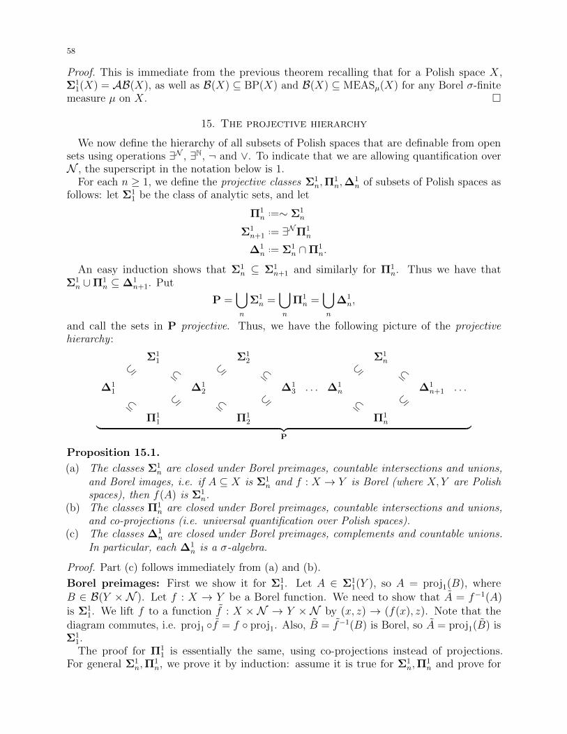
58

Proof. This is immediate from the previous theorem recalling that for a Polish space X,Σ1

1(X) = AB(X), as well as B(X) ⊆ BP(X) and B(X) ⊆ MEASµ(X) for any Borel σ-finitemeasure µ on X. �

15. The projective hierarchy

We now define the hierarchy of all subsets of Polish spaces that are definable from opensets using operations ∃N , ∃N, ¬ and ∨. To indicate that we are allowing quantification overN , the superscript in the notation below is 1.

For each n ≥ 1, we define the projective classes Σ1n,Π

1n,∆

1n of subsets of Polish spaces as

follows: let Σ11 be the class of analytic sets, and let

Π1n..=∼ Σ1

n

Σ1n+1

..= ∃NΠ1n

∆1n..= Σ1

n ∩Π1n.

An easy induction shows that Σ1n ⊆ Σ1

n+1 and similarly for Π1n. Thus we have that

Σ1n ∪Π1

n ⊆∆1n+1. Put

P =⋃n

Σ1n =

⋃n

Π1n =

⋃n

∆1n,

and call the sets in P projective. Thus, we have the following picture of the projectivehierarchy :

Σ11 Σ1

2 Σ1n

⊆ ⊆ ⊆ ⊆ ⊆ ⊆∆1

1 ∆12 ∆1

3 . . . ∆1n ∆1

n+1 . . .

⊆ ⊆ ⊆ ⊆ ⊆ ⊆Π1

1 Π12 Π1

n︸ ︷︷ ︸P

Proposition 15.1.

(a) The classes Σ1n are closed under Borel preimages, countable intersections and unions,

and Borel images, i.e. if A ⊆ X is Σ1n and f : X → Y is Borel (where X, Y are Polish

spaces), then f(A) is Σ1n.

(b) The classes Π1n are closed under Borel preimages, countable intersections and unions,

and co-projections (i.e. universal quantification over Polish spaces).(c) The classes ∆1

n are closed under Borel preimages, complements and countable unions.In particular, each ∆1

n is a σ-algebra.

Proof. Part (c) follows immediately from (a) and (b).

Borel preimages: First we show it for Σ11. Let A ∈ Σ1

1(Y ), so A = proj1(B), whereB ∈ B(Y × N ). Let f : X → Y be a Borel function. We need to show that A = f−1(A)

is Σ11. We lift f to a function f : X × N → Y × N by (x, z) → (f(x), z). Note that the

diagram commutes, i.e. proj1 ◦f = f ◦ proj1. Also, B = f−1(B) is Borel, so A = proj1(B) isΣ1

1.The proof for Π1

1 is essentially the same, using co-projections instead of projections.For general Σ1

n,Π1n, we prove it by induction: assume it is true for Σ1

n,Π1n and prove for

59

Σ1n+1,Π

1n+1 using the same proof as for Σ1

1,Π11, where the set B is assumed to be Π1

n (resp.Σ1n) instead of Borel.

Countable unions and intersections: We will only prove this for Σ1n since it would then

follow for Π1n by taking complements. The closure under countable unions is easily proven by

induction on n because if Ai = proj1(Bi) with Bi ∈ B(X ×N ), then⋃iAi = proj1(

⋃iBi).

To prove the closure under intersections, again let Ai = proj1(Bi) with Bi ∈ B(X ×N ) anduse a coding trick: for x to be in Ai, there has to be a witness yi ∈ N such that (x, yi) ∈ Bi;now we code these witnesses yi into one witness y as follows:

x ∈⋂i

Ai ⇐⇒ ∀i ∈ N ∃yi ∈ N (x, yi) ∈ Bi

⇐⇒ ∃y ∈ N N ∀i ∈ N (x, y(i)) ∈ Bi.

Thus, we are done since N N is homeomorphic to N by N N = (NN)N 'h NN×N 'h NN = N ,where 'h denotes the relation of being homeomorphic.

Borel images: Again the proof is by induction on n. For n = 1 it follows from the definitionof Σ1

1, so suppose it is true for Σ1n, and let X, Y be Polish spaces, A ∈ Σ1

n+1(X), andf : X → Y Borel. We need to show that f(A) is Σ1

n+1. Take B ∈ Π1n(X ×N ) such that

A = proj1(B). By Theorem 5.9, let g : N → X ×N be a continuous surjection. Then wehave

y ∈ f(A) ⇐⇒ ∃x ∈ X(x ∈ A and f(x) = y

)⇐⇒ ∃x ∈ X ∃z ∈ N

((x, z) ∈ B and f(x) = y

)⇐⇒ ∃w ∈ N

(g(w) ∈ B and f(proj1(g(w))) = y

).

The latter condition defines a set in ∃NΠ1n..= Σ1

n+1, so f(A) ∈ Σ1n+1. �

Above we proved various properties of Borel and analytic sets. Using infinite games, weshowed that analytic sets enjoy the PSP and the BP. Similarly, one could also show that theyare universally measurable. This implies that Π1

1 sets also have the BP and are universallymeasurable. However, whether or not all Π1

1 sets satisfy the PSP is already independent fromZFC21. The same is true for Σ1

2 sets regarding all of the regularity properties mentioned, i.e.whether or not Σ1

2 sets have either of the PSP or the BP, or are universally measurable (i.e.measurable with respect to any σ-finite Borel measure), is independent from ZFC.

Proposition 15.2. For any uncountable Polish space Y , Σ1n+1 = ∃Y Π1

n.

Proof. Any such Y is Borel isomorphic to N and Π1n is closed under Borel preimages. �

Proposition 15.3. For any uncountable Polish space X and Polish Y , there is an X-universalset U ⊆ X × Y for Σ1

n(Y ). Same for Π1n.

Proof. We have already constructed this for n = 1, and note that if U is X-universalU ⊆ X×Y for Σ1

n(Y ), then U c is X-universal U ⊆ X×Y for Π1n(Y ). We prove by induction

on n. Suppose that F ⊆ X × Y ×N is an X-universal set for Π1n(Y ×N ). Then clearly

U = proj1,2(F ) is Σ1n+1(Y ), and it is obvious that U parameterizes Σ1

n+1(Y ). �

21Strictly speaking, a large cardinal hypothesis (existence of an inaccessible cardinal) is needed to showthat it is consistent with ZFC that all Π1

1 sets satisfy the PSP. However, the consistency of the failure ofthis statement can be shown in ZFC.

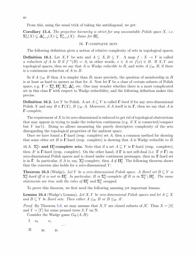
60

From this, using the usual trick of taking the antidiagonal, we get:

Corollary 15.4. The projective hierarchy is strict for any uncountable Polish space X, i.e.Σ1n(X) ( ∆1

n+1(X) ( Σ1n+1(X). Same for Π1

n.

16. Γ-complete sets

The following definition gives a notion of relative complexity of sets in topological spaces.

Definition 16.1. Let X, Y be sets and A ⊆ X,B ⊆ Y . A map f : X → Y is calleda reduction of A to B if f−1(B) = A, in other words, x ∈ A ⇔ f(x) ∈ B. If X, Y aretopological spaces, then we say that A is Wadge reducible to B, and write A ≤W B, if thereis a continuous reduction of A to B.

So if A ≤W B then A is simpler than B; more precisely, the question of membership in Bis at least as hard to answer as that for A. Now let Γ be a class of certain subsets of Polishspace, e.g. Γ = Σ0

ξ ,Π0ξ ,Σ

11,∆

13, etc. One may wonder whether there is a most complicated

set in this class Γ with respect to Wadge reducibility, and the following definition makes thisprecise.

Definition 16.2. Let Y be Polish. A set A ⊆ Y is called Γ-hard if for any zero-dimensionalPolish X and any B ∈ Γ(X), B ≤W A. Moreover, if A itself is in Γ, then we say that A isΓ-complete.

The requirement ofX to be zero-dimensional is enforced to get rid of topological obstructionsthat may appear in trying to make the reduction continuous (e.g. if X is connected/compactbut Y isn’t). Doing so allows measuring the purely descriptive complexity of the setsdisregarding the topological properties of the ambient space.

Once we have found a Γ-hard (resp. complete) set A, then a common method for showingthat some other set B is Γ-hard (resp. complete) is showing that A is Wadge reducible to B.

16.A. Σ0ξ- and Π0

ξ-complete sets. Note that if a set A ⊆ Y is Γ-hard (resp. complete),

then Ac is Γ-hard (resp. complete). On the other hand, if Γ is not self-dual (i.e. Γ 6= Γ) onzero-dimensional Polish spaces and is closed under continuous preimages, then no Γ-hard setis in Γ. In particular, if A is, say, Σ0

ξ-complete, then A /∈ Π0ξ . The following theorem shows

that the converse also holds for a zero-dimensional Y :

Theorem 16.3 (Wadge). Let Y be a zero-dimensional Polish space. A Borel set B ⊆ Y isΣ0ξ-hard iff it is not in Π0

ξ. In particular, B is Σ0ξ-complete iff B is in Σ0

ξ \Π0ξ. The same

statements are true with the roles of Π0ξ and Σ0

ξ swapped.

To prove this theorem, we first need the following amusing yet important lemma:

Lemma 16.4 (Wadge’s Lemma). Let X, Y be zero-dimensional Polish spaces and let A ⊆ Xand B ⊆ Y be Borel sets. Then either A ≤W B or B ≤W Ac.

Proof. By Theorem 5.8, we may assume that X, Y are closed subsets of N . Thus X = [S]and Y = [T ] for some pruned trees S, T on N.

Consider the Wadge game GW (A,B):

I x0 x1

· · ·II y0 y1

61

where xn, yn ∈ N, (xi)i<n ∈ T and (yi)i<n ∈ S for all n. Let x = (xn)n∈N and y = (yn)n∈N.Player II wins iff (x ∈ A↔ y ∈ B).

Note that this game is a usual game with rules with a Borel payoff set since A,B are Borel.Thus, it is determined. Suppose Player II has a winning strategy. We can view this strategyas a monotone map ϕ : T → S such that |ϕ(s)| = |s|, for s ∈ S. By (a) of Proposition 2.9, ϕgives rise to a continuous map ϕ∗ : [S] → [T ]. Since ϕ is a winning strategy for Player II,x ∈ A↔ ϕ∗(x) ∈ B; in other words, A = (ϕ∗)−1(B), so A ≤W B.

Now suppose that Player I has a winning strategy. Note that I wins the above game if(y ∈ B ↔ x /∈ A). Thus, repeating the argument above with roles of the players switched, weget B ≤W Ac. �

Now we are ready to prove the above theorem.

Proof of Theorem 16.3. Because Σ0ξ 6= Π0

ξ , it is clear that if B is Σ0ξ-hard then B is not in

Π0ξ . For the converse, suppose B ⊆ Y is a Borel set not in Π0

ξ and let A ∈ Σ0ξ(X) for some

zero-dimensional Polish X. By Wadge’s lemma, either A ≤W B or B ≤W Ac. The latteralternative cannot happen since it would imply that B ∈ Π0

ξ , which isn’t the case. �

16.B. Σ11-complete sets. Every analytic set in N is a projection of a closed set in N 2.

Identify N 2 with (N×N)N and note that this turns the projection function proj1 : N 2 → Nto p : (N× N)N → NN defined by (xn, yn)n∈N → (xn)n∈N. Recall that closed sets in (N× N)N

are the sets of infinite branches through a tree T on N× N. Thus, a set A ⊆ NN is analyticiff there is a tree T on N× N such that A = p[T ]. (Here we abused the notation and wrotep[T ] instead of p([T ]).)

For a tree T on N× N and x ∈ NN, put

Tx ={s ∈ N<N : (x||s|, s) ∈ T

}and note that Tx is a tree on N. Also note that

x ∈ p[T ] ⇐⇒ [Tx] 6= ∅.This allows us to construct a Σ1

1-complete set.

Definition 16.5. Let T be a tree on a set A. Call T well-founded if the partial order ⊇ onT is well-founded, i.e. there is no infinite chain s0 ( s1 ( s2 ( ... with sn ∈ T . Otherwise,call T ill-founded.

Note that T is well-founded iff [T ] = ∅.We identify P(N<N) with 2N

<Nand thus a tree T on N is an element of 2N

<N. Let Tr

denote the set of trees on N and note that it is a closed subset of 2N<N

and hence Polish. LetIF denote the set of ill-founded trees and note that it is an analytic subset of Tr because forT ∈ Tr,

T ∈ IF ⇐⇒ ∃(sn)n∈N ∈ (N<N)N∀n(sn ∈ T and sn ⊆ sn+1 and |sn| = n).

Proposition 16.6. IF is Σ11-complete.

Proof. Let X be zero-dimensional Polish and A ⊆ X be analytic. By Theorem 5.8, we canidentify X with a closed subset of N . Because closed subsets of N are analytic, A is stillanalytic when viewed as a subset of N , so it is enough to show that (A,N ) ≤W (IF,Tr).

Let T be a tree on N× N such that A = p[T ], so for x ∈ N , we have

x ∈ A ⇐⇒ Tx ∈ IF .

62

Thus, the map N → Tr given by x 7→ Tx is a reduction of A to IF, and it is straightforwardto check that this map is continuous, so we are done. �

63

Part 4. Definable equivalence relations, group actionsand graphs

In the past twenty five years, a major focus of descriptive set theory has been the study ofequivalence relations on Polish spaces that are definable when viewed as sets of pairs (e.g.orbit equivalence relations of continuous actions of Polish groups are analytic). This studyis motivated by foundational questions such as understanding the nature of classificationof mathematical objects (measure-preserving transformations, unitary operators, Riemannsurfaces, etc.) up to some notion of equivalence (isomorphism, conjugacy, conformal equiva-lence, etc.), and creating a mathematical framework for measuring the complexity of suchclassification problems. Due to its broad scope, it has natural interactions with other areasof mathematics, such as ergodic theory and topological dynamics, functional analysis andoperator algebras, representation theory, topology, model theory, etc.

The following definition makes precise what it means for one classification problem to beeasier (not harder) than another.Definition. Let E and F be equivalence relations on Polish spaces X and Y , respectively.We say that E is Borel reducible to F and write E ≤B F if there is a Borel map f : X → Ysuch that for all x0, x1 ∈ X, x0Ex1 ⇐⇒ f(x0)Ff(x1).

We call E smooth (or concretely classifiable) if it Borel reduces to the identity relation Id(X)on some (any) Polish space X (note that such E is automatically Borel). An example of suchan equivalence relation is the similarity relation of matrices; indeed, if J(A) denotes the Jordan

canonical form of a matrix A ∈ Rn2

, then for A,B ∈ Rn2

, we have A ∼ B ⇐⇒ J(A) = J(B).

It is not hard to check that the computation of J(A) is Borel, so J : Rn2 → Rn2

is a Borel

reduction of ∼ to Id(Rn2

), and hence ∼ is smooth. Another (much more involved) exampleis the isomorphism of Bernoulli shifts, which, by Ornstein’s famous theorem, is reduced tothe equality on R by the map assigning to each Bernoulli shift its entropy.

However, many equivalence relations that appear in mathematics are nonsmooth. Forexample, the Vitali equivalence relation Ev on [0, 1] defined by xEvy ⇐⇒ x− y ∈ Q can beeasily shown to be nonsmooth using measure-theoretic or Baire category arguments. Thefollowing theorem (known as the General Glimm–Effros dichotomy, see [HKL90]) shows thatin fact containing Ev is the only obstruction to smoothness:

Theorem (Harrington–Kechris–Louveau ’90). Let E be a Borel equivalence relation on aPolish space X. Then either E is smooth, or else Ev vB E.22

This was one of the first major victories of descriptive set theory in the study of equivalencerelations. It in particular implies that Ev is the easiest among all nonsmooth Borel equivalencerelations in the sense of Borel reducibility. Besides its foundational importance in the theoryof Borel equivalence relations, it also generalized earlier important results of Glimm andEffros. By now, many other dichotomy theorems have been proved and general methods ofplacing a given equivalence relation among others in the Borel reducibility hierarchy have

22Here, vB means that there is an injective Borel reduction.

64

been developed. However, there are still many fascinating open problems left and the Borelreducibility hierarchy is yet to be explored.

Another very active area of descriptive set theory is combinatorics of definable graphs, inparticular, coloring problems of various classes of definable graphs on Polish spaces. Thereare dichotomy theorems known for graph colorings as well, and they are tightly connected tothe dichotomy theorems for equivalence relations. Below, we will discuss the first dichotomytheorem for graphs by Kechris–Solecki–Todorcevic [KST99].

17. Examples of equivalence relations and Polish group actions

17.A. Equivalence relations. Let X denote a Polish space. We start by listing somefamiliar examples of equivalence relations that appear in various areas of mathematics.

Examples 17.1.

(a) The identity (equality) relation Id(X) on X is a closed equivalence relation.

(b) The Vitali equivalence relation Ev on [0, 1], defined by xEvy :⇔ x− y ∈ Q, is clearly anFσ equivalence relation.

(c) Define the equivalence relation E0(X) on XN of eventual equality of sequences, namely:

for x, y ∈ XN, xE0(X)y :⇔ ∀∞n(x(n) = y(n)). This is again an Fσ equivalence relation.Important special cases when X = 2, i.e. XN = C, and when X = N . In the first casewe simply write E0

..= E0(2) and in the second case we write E1..= E0(N ).

(d) The similarity relation ∼ of matrices on the space Mn(C) of n × n matrices: forA,B ∈Mn(C), A ∼ B ⇔ ∃Q ∈ GLn(C) QAQ−1 = B. By definition, this is an analyticequivalence relation, but we will see below that it is actually Borel.

(e) Consider the following subgroups of RN under addition:

• `p ={x ∈ RN :

∑n |x(n)|p <∞

}, for 1 ≤ p <∞,

• `∞ ={x ∈ RN : supn |x(n)| <∞

},

• c0 ={x ∈ RN : limn x(n) = 0

}.

The first two are Fσ subsets of RN and the last is Π03. Thus, if I is one of these

subgroups, then the equivalence relation EI on RN, defined by

xEIy :⇔ x− y ∈ I ,

is Fσ for I = `p, 1 ≤ p ≤ ∞, and is Π03 for I = c0.

(f) Fix a countable first-order relational language L = {Ri}i∈N, where Ri is a relationsymbol of arity ni. The set of countable L-structures can be turned into a Polish spaceby fixing their underlying set to be N and, for each i, identifying the interpretation ofRi (i.e. a relation on Nni) with its characteristic function. Such a structure is simply anelement of XL ..=

∏i∈N 2N

ni . This allows talking about the Polish spaces of countableorderings and countable graphs, for example. Also, because any first-order language canbe turned into a relational language by replacing function symbols with relation symbolsfor their graphs, we can also consider Polish spaces of countable groups, rings, fields, etc.

Thus, isomorphism of countable L-structures, denoted by 'L, naturally falls intothe framework of descriptive set theory as it is an analytic equivalence relation on XL;

65

indeed, two structures are isomorphic if and only if there exists a certain bijection ffrom N to N, i.e. a certain element f ∈ N .

17.B. Polish groups. Many natural analytic equivalence relations arise as orbit equivalencerelations of continuous (or Borel) actions of Polish groups.

Definition 17.2. A topological group is a group with a topology on it so that groupmultiplication (x, y) → xy and inverse x → x−1 are continuous functions. Such a group iscalled Polish if its topology happens to be Polish.

Here are some important examples of Polish groups.

Examples 17.3.

(a) All countable groups with the discrete topology are Polish. In fact, it is an exercise toshow that the only Polish topology on a countable group is the discrete topology.

(b) The unit circle S1 ⊆ C is a Polish group under multiplication.

(c) Rn,RN, (Z/2Z)N are Polish groups under coordinatewise addition (note that the latter isjust the Cantor space C).

(d) The group S∞ of permutations of N (i.e. bijections from N to N) is a Gδ subset of N ,so is a Polish group with the relative topology.

(e) Let (X,B, µ) be a standard probability space, i.e. (X,B) is a standard Borel space andµ is a probability measure on B; we will often simply write (X,µ). A measure-preservingautomorphism of (X,µ) is a bimeasurable23 bijection T : X → X such that for everymeasurable A ⊆ X, µ(T−1(A)) = µ(A). For example, take X = [0, 1) with the Lebesguemeasure and let Tα : X → X be the translation modulo 1 by a real α ∈ (0, 1).

Let Aut(X,µ) denote the set of all measure-preserving automorphisms up to a.e.equality. This is clearly a group under composition and we equip it with the so-calledweak topology defined in terms of convergent sequences as follows:

Tn → T :⇔ ∀A ∈ B µ(Tn(A)∆T (A))→ 0.

One can show that this is indeed a Polish topology, making Aut(X,µ) a Polish group.

(f) Let H be a separable Hilbert space and let U(H) denote the group of unitary operatorson H, i.e. invertible linear operators U : H → H that preserve the inner product(equivalently, U∗ = U−1). This is a Polish group under the strong operator topology24

defined in terms of convergent sequences as follows:

Un → U :⇔ ∀h ∈ H ||Un(h)− U(h)||H → 0.

23Bimeasurable means both T and T−1 are measurable.24The strong and weak operator topologies (defined on the space B(H) of bounded operators on H)

coincide on U(H).

66

17.C. Actions of Polish groups.

Definition 17.4. Let G be a Polish group and X be a Polish space. An action a : Gy Xof G on X is said to be continuous (resp. Borel) if the action function a : G×X → X givenby (g, x) 7→ g ·a x is continuous (resp. Borel).

We denote by EG (or sometimes by Ea) the orbit equivalence relation induced by such anaction. Note that EG is analytic because for x, y ∈ X,

xEGy ⇐⇒ ∃g ∈ G(g ·a x = y).

Here we list some examples of continuous actions of Polish groups.

Examples 17.5.

(a) Any Polish group acts on itself by left multiplication, as well as by conjugation. Itfollows from the definition of topological groups that these actions are continuous.

(b) Let G be a Polish group and H < G be a Polish (equivalently, closed) subgroup. The leftmultiplication action of H on G is clearly continuous and the induced orbit equivalencerelation EH is the relation of being in the same right H-coset, i.e. xEHy ⇔ Hx = Hy.We refer to EH as the H-coset equivalence relation.

(c) The Vitali equivalence relation Ev is exactly the orbit equivalence relation of the transla-tion action of Q on R.

(d) The relation E0 of eventual equality on C is induced by a continuous action of a countable

group as follows: for each n ∈ N, let σn : C → C be the map that flips the nth bit:

σn(x)(i) ..=

{1− x(i) if i = nx(i) otherwise,

and let Γ be the group generated by {σn : n ∈ N}, which is just the direct sum⊕

n∈N Z/2Z.It is clear that each σn is a homeomorphism of C and EΓ = E0.

One can also show that, after throwing away two orbits (more precisely, restricting E0

to C ′ = {x ∈ C : x has infinitely many 0-s and 1-s}), we can realize E0 by a continuousaction of Z known as the odometer action. We leave this as an exercise.

(e) A rotation of S1 is simply an action Z y S1, where 1 ∈ Z acts as multiplication by eαπi,for a fixed α ∈ R. Clearly this action is continuous and we denote the orbit equivalencerelation by Eα.

(f) The equivalence relations E0,Ev,Eα are examples of countable equivalence relations. Ingeneral, orbit equivalence relations induced by continuous or Borel actions of countablegroups are examples of countable Borel (why?) equivalence relations. Curiously enough,these are all of the examples! More precisely, any countable Borel equivalence relationarises as the orbit equivalence relation of a Borel action of a countable group. This is atheorem by Feldman and Moore, and we will prove it below.

(g) The similarity relation ∼ of matrices in Mn(R) is induced as the orbit equivalencerelation of the conjugation action of GLn(R) on Mn(R).

(h) For a first-order relational language L, the group S∞ admits a natural action on the Polishspace XL of countable L-structures by permuting their underlying sets. Clearly, theinduced orbit equivalence relation is exactly the relation of isomorphism of L-structures.

67

(i) For a standard probability space (X,B, µ), let MALG denote the σ-algebra of µ-measurable sets modulo the σ-ideal of µ-null sets. The metric d(A,B) ..= µ(A 4 B)on MALG is complete and the fact that B is countably generated implies that it isseparable, so MALG is a Polish space and the natural action of Aut(X,µ) on MALG isby isometries. It also follows that this action is continuous.

(j) Similarly, for a separable Hilbert space H, the natural action of U(H) on H is continuous.

18. Borel reducibility

Let E and F be equivalence relations on Polish spaces X and Y , respectively. The followingdefines the class of functions from X to Y that induce functions from X/E to Y/F .

Definition 18.1. A function f : X → Y is called a homomorphism from E to F if for allx0, x1 ∈ X,

x0Ex1 ⇒ f(x0)Ff(x1).

f : X → Y is called a reduction of E to F if for all x0, x1 ∈ X,

x0Ex1 ⇔ f(x0)Ff(x1).

Note that reductions induce injections X/E ↪→ Y/F .

The following makes it precise what it means for a classification problem in mathematicsto be easier (not harder) than another classification problem:

Definition 18.2. Let E and F be equivalence relations on Polish spaces X and Y , respectively.We say that E is Borel reducible to F , and write E ≤B F , if there is a Borel reduction ofE to F . Furthermore, we say that E is strictly below F , and write E <B F , if E ≤B F butF �B E.

The choice of “Borel” as the regularity condition on the reduction is mainly because anytwo uncountable Polish spaces are Borel isomorphic, so the existence of Borel reductions doesnot depend on the particular choice of the underlying Polish spaces and it only depends onthe inherent complexity of the equivalence relations, which is what we want to measure.

We replace the subscript B in ≤B by c if there is a continuous reduction, and we write vinstead of ≤ if the reduction is injective.

It is clear that ≤B is a quasi-order25 on the class of all equivalence relations on Polishspaces26. We call E and F Borel bireducible, and write E ∼B F , if E ≤B F and F ≤B E.Since Borel reductions induce Borel embeddings X/E ↪→ Y/E, we refer to the bireducibilityclass of E as the Borel cardinality of X/E.

We also call E and F Borel isomorphic, and write E 'B F , if there is a bijective Borelreduction (thus a Borel isomorphism from X to Y ) of E to F .

Remark 18.3. In general, E vB F and F vB E does not imply E 'B F ; more precisely, theSchroder–Bernstein argument doesn’t work unless both reductions are “locally surjective onclasses”. The latter means that the Borel reduction f : X → Y has the property that forevery x ∈ X, f([x]E) is an entire F -class, i.e. f([x]E) = [f(x)]F . Indeed, imagine a situationof having injective Borel reductions f : X ↪→ Y and g : Y ↪→ X of E to F and F to E,

25Quasi-order is a reflexive and transitive relation, not necessarily antisymmetric.26This is actually a set if we fix a particular uncountable Polish space, which we can do as any two of

them are Borel isomorphic.

68

respectively, such that for some x ∈ X, [x]E ∩ g(Y ) = ∅ and f([x]E) ( [f(x)]F . Then, theSchroder–Bernstein argument would map the elements of [x]E by f into [f(x)]F and theelements in [f(x)]F \ f([x]E) by g into [g(f(x))]E. But [g(f(x))]E 6= [x]E because [x]E isdisjoint from [g(Y )]F , so the elements in f([x]E) would go to a different E-class (namely, [x]E)than the elements in [f(x)]F \ f([x]E), and hence, the resulting map will not be a reduction.

The systematic study of the Borel reducibility hierarchy of definable equivalence relationsis sometimes referred to as invariant descriptive set theory. It was pioneered by Silver,Harrington, Kechris, Louveau, and others, in the late ’80s and early ’90s. The goal ofinvariant descriptive set theory is to understand the Borel reducibility hierarchy (and hence,the complexity of classification problems that appear in many areas of mathematics suchas analysis, ergodic theory, operator algebras, model theory, recursion theory, etc.), andto develop methods for placing a given equivalence relation into its “correct” spot in thishierarchy.

19. Perfect set property for quotient spaces

Given a definable equivalence relation E on a Polish space X, first thing one would want toknow about the quotient space X/E is its cardinality. A strengthening of this is the questionof whether or not X/E has the perfect set property and the following definition makes itprecise:

Definition 19.1. We say that E has perfectly many classes if Id(C) vc E.

Proposition 19.2. For an equivalence relation E on a Polish space X,

Id(C) vc E ⇐⇒ Id(C) vB E ⇐⇒ Id(C) ≤B E.

Proof. Left as an exercise. �

Proposition 19.3. Let E be an analytic or co-analytic equivalence relation on a Polish spaceX. If E has countably many equivalence classes, then E is Borel and hence E ≤B Id(N).

Proof. Say E is analytic (the proof is the same for co-analytic), and hence, so is each E-class(being a fiber of E). But the complement of each E-class C is a countable union of E-classes,so is analytic as well. Thus, C is ∆1

1 and hence is Borel. Letting {xn}n<k, k ≤ ω, be a set ofrepresentatives of the E-classes (one from each), we see that for all x, y ∈ X,

xEy ⇔ ∃n < k (x, y ∈ [xn]E).

This shows that E is Borel since each [xn]E is Borel. Moreover, the function that maps allelements of [xn]E to n is a Borel map from X to k witnessing E ≤B Id(k) vc Id(N). �

In the light of last two propositions, the question of whether X/E has the perfect setproperty is the same as whether

Id(N) <B E <B Id(C).

We give some answers to this question in the next subsections.

69

19.A. Co-analytic equivalence relations: Silver’s dichotomy. In 1980, Silver showedthat the perfect set property holds for Π1

1 equivalence relations, namely:

Dichotomy 19.4 (Silver ’80). Any co-analytic equivalence relation E on a Polish space Xhas either countably many or perfectly many classes. In other words, either E ≤B Id(N), orId(C) ≤B E.

Silver’s original proof was quite complicated and used forcing. Later on Harrington reprovedit using a finer topology (not Polish) on X that comes from recursion theory, the so-calledGandy–Harrington topology. Finally, in 2008, Ben Miller found a classical proof (using onlyBaire category arguments) of a dichotomy theorem by Kechris–Solecki–Todorcevic aboutBorel colorings of analytic graphs, and from this he deduced Silver’s dichotomy (and otherdichotomies as well). We will give this proof later on in the notes.

19.B. Analytic equivalence relations: Burgess’ trichotomy. The perfect set propertydoes not hold for analytic equivalence relations! For example, let LO denote the Polish spaceof all linear orderings (this is a closed subset of XL, with L = {<}), let WO ⊆ LO denote theset of all well-orderings, and define an equivalence relation E on LO as follows: for x, y ∈ LO,

xEy :⇔ (x /∈WO∧y /∈WO) ∨ (x ' y),

where ' stands for isomorphism of orderings. E is clearly analytic since WO is co-analytic(it is an exercise to show that WO is actually Π1

1-complete) and ' is analytic (isomorphismof structures is analytic because it holds when there exists a certain bijection from N to N).All non-well-orderings in LO are E-equivalent (belong to one E-class) and there are preciselyω1-many nonisomorphic wellorderings of N. Thus, E has exactly ω1-many classes and henceif the continuum hypothesis doesn’t hold, E won’t have the perfect set property.

So what are the possibilities for the cardinality of X/E for a given analytic E?

Trichotomy 19.5 (Burgess ’78). Any analytic equivalence relation E on a Polish space Xhas either countably many, ω1-many, or perfectly many classes.

We won’t prove this theorem in these notes, but the proof can be found in [Gao09].

The Vaught conjecture. Let L be a countable language and let T be first-order L-theory, i.e.a set of L-sentences. A straightforward induction on the length of formulas in T shows thatthe set Mod(T ) of countable models of T is a Borel subset of XL.

Vaught conjecture. Any countable first-order theory T has either countably many orperfectly many nonisomorphic countable models.

As mentioned above, the isomorphism relation of countable structures is precisely the orbitequivalence relation ES∞ induced by the natural action of S∞ on XL. Thus, the Vaughtconjecture is simply the statement that Silver’s dichotomy holds for ES∞|Mod(T ), and it hasthe following generalization (a present from model theory to descriptive set theory):

Topological Vaught conjecture. Borel actions of Polish groups on Polish spaces haveeither countably many or perfectly many orbits.

The best currently known result in this direction is a theorem of Becker stating thattopological Vaught conjecture holds for the so-called cli groups, i.e. Polish groups that admita complete left-invariant metric.

70

19.C. Meager equivalence relations: Mycielski’s theorem. Many interesting equiva-lence relations have small equivalence classes and the following proposition shows that theseare exactly the meager equivalence relations.

Proposition 19.7. Let E be an equivalence relation on a Polish space X having the BP.Then E is meager if and only if each E-class is meager.

Proof. Implication ⇐ is by the Kuratowski–Ulam theorem. For ⇒, the Kuratowski–Ulamtheorem merely gives

∀∗x ∈ X ([x]E is meager), (∗)so a priori there may be an x0 ∈ X with [x0]E non-meager. But then, since for every x ∈ [x0]E,[x]E = [x0]E, the set

A = {x ∈ X : [x]E is non-meager}contains [x0]E, so is non-meager, contradicting (∗). �

Examples 19.8.

(a) All countable27 Borel equivalence relations on nonempty perfect Polish spaces are meager.This includes E0, Ev, the irrational rotation Eα, and in general, any orbit equivalencerelation induced by a Borel action of a countable group.

(b) For any Polish space X with |X| ≥ 2, the equivalence relation E0(X) of eventual equality

on XN is meager; in particular, E1 = E0(N ) is meager. This is because for each x ∈ XN,[x]E0(X) =

⋃nAn, where An ..= {y ∈ Y : ∀k ≥ n y(k) = x(k)} is nowhere dense (has

empty interior and is closed).

(c) The equivalence relations EI for I = c0 or `p, 1 ≤ p ≤ ∞. This is because everyEI equivalence class is homeomorphic to I , c0 ⊆ `p ⊆ `∞, and `∞ is meager because`∞ =

⋃nAn, where An ..=

{x ∈ RN : supn |x(n)| ≤ n

}is nowhere dense (has empty

interior and is closed).

Note that since each equivalence class of a meager equivalence relation (with the BP) ismeager, there must be uncountably many classes. In fact, we have:

Theorem 19.9 (Mycielski). Any meager equivalence relation E on a Polish space X hasperfectly many classes.

Proof. Write E =⋃n Fn, where each Fn ⊆ X × X is nowhere dense and Fn ⊆ Fn+1. In

order to get a desired embedding C ↪→ X, we will construct a Cantor scheme (Us)s∈2<N on Xof vanishing diameter (with respect to a fixed complete metric d for X) with the followingproperties:

(i) Us is nonempty open and Usai ⊆ Us, for each s ∈ 2<N, i ∈ {0, 1};(ii) (Us × Ut) ∩ Fn = ∅, for all distinct s, t ∈ 2n and n ∈ N.

Granted this construction, let f : C ⇀ X be the associated map. By Proposition 5.4, thedomain of f is all of C, and f is continuous and injective. Hence f is a topological embeddingsince C is compact. To show that f is also a reduction of Id(C) to E, we need to fix distinctσ, τ ∈ C and show that (f(σ), f(τ)) /∈ E. To this end, let k ∈ N be such that σ|n 6= τ |n, for

27We call an equivalence relation countable if every equivalence class is countable; not to be confused withthe number of equivalence classes being countable.

71

all n ≥ k. But for each n ≥ k, f(σ) ∈ Uσ|n and f(τ) ∈ Uτ |n , so by (ii), (f(σ), f(τ)) /∈ Fn.Since the Fn are increasing, (f(σ), f(τ)) /∈ Fn for all n < k as well, so (f(σ), f(τ)) /∈ E.

To construct such a scheme, first note that X is perfect: indeed, if x ∈ X is an isolatedpoint, then {(x, x)} is open in X2 and {(x, x)} ⊆ E, contradicting E being meager. Thisallows us to construct a Cantor scheme with property (i) as done in the proof of the perfectset theorem for Polish spaces. As for (ii), one has to iteratively use the following fact: fora nowhere dense set F ⊆ X2 and any nonempty open sets U, V ⊆ X, there are nonemptyopen sets U ′ ⊆ U and V ′ ⊆ V such that (U ′ × V ′) ∩ F = ∅. We leave the details of thisconstruction as an exercise. �

20. Concrete classifiability (smoothness)

In this section we make it precise what it means to classify mathematical objects (matrices,measure-preserving transformations, unitary operators, Riemann surfaces, etc.) up to somenotion of equivalence (isomorphism, conjugacy, conformal equivalence, etc.). We will considersome examples and nonexamples, as well as discuss related (famous) dichotomy theorems.

20.A. Definitions.

Definition 20.1. An equivalence relation E on a Polish space X is called concretely classifi-able (or smooth) if E ≤B Id(R). By the Borel isomorphism theorem, R can be replaced byany other uncountable Polish space.

Note that smooth equivalence relations are necessarily Borel : indeed, if f : X → R is aBorel reduction of E to Id(R), then the function f2 : X2 → R2 by (x, y) 7→ (f(x), f(y)) isBorel and E = f−1

2 (∆R), where ∆R is the diagonal in R2. But ∆R is closed in R2, so E isBorel being a preimage of Borel.

A special case of smoothness is when we can select a canonical representative from eachequivalence class.

Definition 20.2. Let E be an equivalence relation on a Polish space X. A map s : X → Xis called a selector for E if for all x ∈ X, s(x) ∈ [x]E, and s is a reduction of E to Id(X), i.e.xEy ⇔ s(x) = s(y). A set Y ⊆ X is called a transversal for E if it meets every E-class atexactly one point, i.e. for each x ∈ X, [x]E ∩ Y is a singleton.

Proposition 20.3. An analytic equivalence relation E on a Polish space X admits a Borelselector if and only if it admits an analytic transversal.28

Proof. If s : X → X is a Borel selector for E, then it is clear that s(X) is an analytictransversal. For the converse, let Y ⊆ X be an analytic transversal and define s : X → X byx 7→ the unique y ∈ Y with xEy. To prove that s is Borel, we fix a Borel set B ⊆ X andshow that s−1(B) is Borel. Note that s−1(B) = [B ∩ Y ]E and hence is analytic. But also(s−1(B))c = s−1(Bc) = [Bc ∩ Y ]E, so (s−1(B))c is also analytic, and thus s−1(B) is Borel. �

Thus, the chain of implications for analytic equivalence relations is as follows:

Borel transversal ⇒ analytic transversal ⇔ Borel selector ⇒ smooth.

Concerning the reverse direction of the first implication, we have the following:

28Thanks to Aristotelis Panagiotopoulos for pointing out that assuming the existence of a merely analytictransversal still implies the existence of a Borel selector.

72

Proposition 20.4. For orbit equivalence relations of Borel actions of Polish groups, anyanalytic transversal is actually Borel.

Proof. Let Gy X be a Borel action of a Polish group G on a Polish space X, and let Y ⊆ Xbe an analytic transversal for EG. Then, for x ∈ X,

x /∈ Y ⇐⇒ ∃g ∈ G (gx ∈ Y and gx 6= x),

so Y c is analytic as well, and hence Y is Borel by Souslin’s theorem (Corollary 12.7). �

As for the implication “Borel selector ⇒ smooth”, it is a theorem of Burgess that thereverse implication is also true for the orbit equivalence relations of continuous actions ofPolish groups. Here we will record a special case of this29.

Definition 20.5. An equivalence relation E on a Polish space X is called countable if eachE-class is countable.

Proposition 20.6. A countable equivalence relation E on a Polish space X is smooth if andonly if it admits a Borel selector.

Proof. The nontrivial direction follows immediately from Corollary 13.8. �

20.B. Examples of concrete classification. We start by listing some well known examplesof equivalence relations from different areas of mathematics that admit concrete classification.

Examples 20.7.

(a) Isomorphism of finitely generated abelian groups. Let Lg = {·, 1} be the language ofgroups. Then the set Y ⊆ XLg of all finitely generated abelian groups is Σ0

3 (∃ finitelymany elements such that ∀ group elements γ ∃ a combination equal to γ), and hencestandard Borel. We know from algebra that every Γ ∈ Y is isomorphic to a group of theform Zn

⊕Zq1⊕Zq2⊕

...⊕Zqk , where q1 ≤ q2 ≤ ... ≤ qk are powers of primes. The

map Γ 7→ Zn⊕Zq1⊕Zq2⊕

...⊕Zqk from Y to Y is a selector for Iso(Y ) and it can

be shown to be Borel, witnessing the smoothness of Iso(Y ).

(b) Similarity of matrices. Let Mn(C) denote the Polish space of complex n× n matricesand ∼ denote the similarity relation on Mn(C), which is Σ1

1 by definition. For eachA ∈ Mn(C), let J(A) denote its Jordan canonical form. We know from linear algebrathat A ∼ B ⇔ J(A) = J(B), in other words, J is a selector for ∼. Moreover, one canshow that it is Borel, so ∼ is smooth. In particular, ∼ is a Borel equivalence relation,which wasn’t apparent at all from its definition.

(c) Isomorphism of Bernoulli shifts. Let (X,µ) be a probability space (X can be finite)

and let µZ denote the product measure on XZ. Let S : XZ → XZ denote the shiftautomorphism, i.e. for f ∈ XZ and n ∈ Z, T (f)(n) = f(n− 1). The dynamical system(XZ, µZ, S) is called a Bernoulli shift. By the measure isomorphism theorem, everyBernoulli shift is isomorphic to ([0, 1], λ, T ), where λ is the Lebesgue measure and Tsome measure-preserving automorphism of ([0, 1], λ). In this case, we would call Ta Bernoulli shift as well, and let B ⊆ Aut([0, 1], λ) be the set of all Bernoulli shifts.Ornstein showed that B is a Borel subset of Aut([0, 1], λ), and hence is a standardBorel space. Furthermore, to each T ∈ Aut([0, 1], λ), one can attach a real numbere(T ) ∈ R∪ {∞} called the entropy of the dynamical system ([0, 1], λ, T ), which somehow

29The fact this is a special case is due to the Feldman–Moore theorem 22.2 and Corollary 11.21

73

measures the probabilistic unpredictability of the action of T . This notion of entropyis defined by Kolmogorov and it follows from the definition that it is an isomorphisminvariant. For the Bernoulli shifts however (i.e. T ∈ B), it is a celebrated theoremof Ornstein that entropy is a complete invariant! In other words, for T1, T2 ∈ B,([0, 1], λ, T1) ' ([0, 1], λ, T2)⇔ e(T1) = e(T2). It can also be checked that the functionT 7→ e(T ) is Borel, hence a Borel reduction of the isomorphism relation of Bernoullishifts to Id(R ∪ {∞}), witnessing the smoothness of the former.

The following proposition gives a new batch of examples.

Proposition 20.8. Let E be an equivalence relation on a Polish space X. If each E-class isGδ and the E-saturations of open sets are Borel, then E is smooth. Moreover, if each E-classis actually closed, then E admits a Borel selector.

Proof. The map ρ : X → F (X) by x 7→ [x]E is a reduction of E to Id(F (X)) because if

[x]E = [y]E, then both [x]E, [y]E are dense Gδ subsets of [x]E, hence comeager in [x]E (in the

relative topology of [x]E). By the Baire category theorem, [x]E ∩ [y]E 6= ∅, so [x]E = [y]E.It remains to show that ρ is Borel, which follows from the fact that if U ⊆ X is open, thenρ−1({F ∈ F (X) : F ∩ U 6= ∅}) = [U ]E is Borel by the hypothesis.

If moreover, each E-class is closed, then composing ρ with a Borel selector for F (X) (seeTheorem 13.16) gives a Borel selector for E. �

Lemma 20.9. Let G be a group and let it act Gy X by homeomorphisms on a Polish spaceX. Then the saturations of open subsets of X are open.

Proof. For open U ⊆ X, [U ]G =⋃g∈G gU is open because each gU is open being a homeo-

morphic image of U . �

This lemma, together with the above proposition, gives:

Corollary 20.10. Let a group G act by homeomorphisms on a Polish space X and let EGdenote the induced orbit equivalence relation. If every orbit is Gδ, then EG is smooth. Ifevery orbit is closed, then EG admits a Borel selector.

Examples 20.11.

(a) Orbit equivalence relation EK induced by a continuous action of a compact group K on aPolish space X admits a Borel selector. This is because every orbit [x]K is equal to K · x,and hence is compact being a continuous image of a compact space K. In particular,[x]K is closed.

(b) For a closed subgroup H < G of a Polish group G, the H-coset equivalence relation EHadmits a Borel selector. Indeed, each EH-class is just an H-coset Hg, for some g ∈ Gand hence is closed.

(c) For a discrete subgroup Γ < G of a Polish group G, the Γ-coset equivalence relation EΓ

admits a Borel selector. This is a special case of the previous example because discretesubgroups of Polish groups are closed. Indeed, the relative topology of Γ is discrete andhence Polish. But by a homework exercise, Polish subgroups of Polish groups are closed.

As an instance of the last example, the Z-coset equivalence relation on R in fact admits aBorel transversal, namely, the interval [0, 1).

74

20.C. Characterizations of smoothness.

Definition 20.12. Let E be an equivalence relation on a Polish space X and let F be afamily of subsets of X. We say that F generates E if

xEy ⇐⇒ ∀A ∈ F (x ∈ A⇔ y ∈ A).

Theorem 20.13 (Combinatorial characterization of smoothness). An equivalence relation Eon a Polish space X is smooth if and only if it is generated by a countable Borel family.

Proof. For the forward direction, let f : X → R be a Borel reduction of E to Id(R) and let{Un}n be a countable open basis for R. Then it is easy to check that the family {f−1(Un)}ngenerates E.

Conversely, if {Bn}n is a countable Borel family generating E then it is easy to check thatthe function f : X → C, defined by x 7→ the characteristic function of {n ∈ N : x ∈ Bn}, is aBorel reduction of E to Id(C). �

Using this, one also gets:

Theorem 20.14 (Topological characterization of smoothness). An equivalence relation Eon a Polish space (X, T ) is smooth if and only if there is a Polish topology TE ⊇ T on X(and hence automatically B(TE) = B(T )) such that E is closed in (X2, T 2

E ).

Proof. Outlined in a homework problem. �

The following proposition gives a class of examples of closed equivalence relations on Polishspaces.

Proposition 20.15. Orbit equivalence relations induced by continuous actions of compactgroups are closed.

Proof. Let G be a compact group, X a topological space and consider a continuous actionGy X, i.e. a : G×X → X is continuous. Then the graph Graph(a) of the function a is aclosed subset of G×X2 and EG = proj2,3(Graph(a)). Therefore, EG is closed by the tube

lemma30 since G is compact. �

20.D. Nonsmooth equivalence relations.

Definition 20.16. An equivalence relation E on a Polish space X (resp. measure space(X,B, µ)) is called generically ergodic (resp. µ-ergodic) if every invariant subset of X withthe BP (resp. µ-measurable) is either meager (resp. µ-null) or comeager (resp. µ-conull).

We call a (continuous or measurable) group action G y X generically ergodic (resp.µ-ergodic) if such is the induced orbit equivalence relation EG.

Proposition 20.17. Let E be an equivalence relation on a Polish space X and let f : X → Cbe a Baire measurable homomorphism of E to Id(C). If E is generically ergodic, then thereis y ∈ C such that f−1(y) is comeager. Letting µ be a Borel measure on X, the analogousstatement holds for µ-ergodic E.

30The tube lemma states that for topological spaces K,Y , if K is compact then projections of closedsubsets of K × Y onto Y are closed.

75

Proof. We only prove the topological statement since the proof of the measure-theoreticstatement is analogous. First note that for any A ⊆ C, f−1(A) is E-invariant by the virtueof f being a homomorphism. By recursion on n, we now define an increasing sequence(sn)n ⊆ 2<N such that |sn| = n and f−1(Nsn) is comeager. Put s0 = ∅, and suppose sn isdefined and satisfies the requirements. Since f−1(Nsn) = f−1(Nsna0) ∪ f−1(Nsna1), for atleast one i ∈ {0, 1}, f−1(Nsnai) must be nonmeager, and hence comeager because f−1(Nsnai)is invariant and has the BP. Set sn+1 = sn

ai. Having finished the construction of (sn)n, puty =

⋃n sn. Then f−1(y) = f−1(

⋂nNsn) =

⋂n f−1(Nsn) is comeager. �

Corollary 20.18. Let E be an equivalence relation on a Polish space X. If E is genericallyergodic (resp. ergodic) and every E-class is meager, then E is not smooth. Letting µ be anontrivial Borel measure on X, the analogous statement holds for µ-ergodic E.

Proof. If f : X → C is a Baire measurable reduction of E to Id(C), then the preimage of everypoint y ∈ f(X) is an E-class, and hence is meager, contradicting the previous proposition. �

Proposition 20.19. Let Γ be a group acting on a Polish space X by homeomorphisms, i.e.each γ ∈ Γ acts as a homeomorphism of X. The following are equivalent:

(1) EΓ is generically ergodic.(2) Every invariant nonempty open set is dense.(3) For comeager-many x ∈ X, the orbit [x]Γ is dense.(4) There is a dense orbit.(5) For every nonempty open sets U, V ⊆ X, there is γ ∈ Γ such that (γU) ∩ V 6= ∅.

Proof. The only implications worth proving are the following:(2)⇒(3): Fixing a countable basis {Un}n, note that D ..=

⋂n[Un]Γ is comeager and for every

x ∈ D, the orbit [x]Γ intersects every Un, so is dense.(5)⇒(1): Let A ⊆ X be invariant and have the BP. If neither of A,Ac are meager, then,by the Baire alternative, there are nonempty open sets U, V such that U A and V Ac.Let γ ∈ Γ be such that W ..= (γU) ∩ V 6= ∅. Because γ is a homeomorphism, γU γAand hence γU A because γA = A. Thus, W A and W Ac, contradicting W beingnonmeager. �

Corollary 20.20. If a group Γ acts by homeomorphisms on a Polish space X such that everyorbit is meager (e.g. when Γ is countable and X is perfect) and there is a dense orbit, then EΓ

is nonsmooth. In particular, if G is a Polish group and Γ < G is a countable dense subgroup,then the orbit equivalence relation EΓ of the left translation action Γ y G is nonsmooth.

Proof. The second statement is immediate from the first, and the first statement follows fromCorollary 20.18 and Proposition 20.19. �

Examples 20.21.

(a) The Vitali equivalence relation Ev is nonsmooth. Indeed, Ev is the orbit equivalencerelation of the translation action of Q on R.

(b) The irrational rotation Eα of S1 is nonsmooth. Indeed, let Γ be the subgroup of S1

generated by e2παi. It is clear that Eα is precisely the orbit equivalence relation inducedby the translation action Γ y S1, and it follows from irrationality of α that Γ is dense.

76

(c) E0 is nonsmooth. Indeed, each E0-class is countable dense and E0 is induced by acontinuous action of a countable group as described in Example 17.5(d). Moreover, likein the previous two examples, we can even view E0 as the orbit equivalence relationinduced by the translation action of a countable dense subgroup Γ < (Z/2Z)N, namely,Γ = (Z/2Z)⊕N ..=

{q ∈ (Z/2Z)N : ∀∞n q(n) = 0

}.

It follows from Silver’s dichotomy (or Mycielski’s theorem for Ev,Eα,E0) that all Borelnonsmooth equivalence relations E are strictly above Id(C) in the Borel reducibility hierarchy;in particular, Id(C) <B Ev,Eα,E0.

20.E. General Glimm–Effros dichotomies. For an equivalence relation E on a Polishspace X, it is clear that if E0 ≤B E then E is nonsmooth. The following striking theoremshows that this is the only impediment to smoothness!

Dichotomy 20.22 (Harrington–Kechris–Louveau ’90). For any Borel equivalence relationE on a Polish space X, either E is smooth or E0 vc E.

This theorem shows, in particular, that E0 is the ≤B-minimum element (up to ∼B) amongall nonsmooth Borel equivalence relations; in other words, it is the minimum unsolvableclassification problem among the Borel ones. Moreover, an application of Mycielski’s theoremto E0 gives Id(C) <B E0 vc E, for any Borel nonsmooth equivalence relation E.

Because orbit equivalence relations induced by continuous actions of Polish groups are ingeneral analytic, the Harrington–Kechris–Louveau dichotomy doesn’t apply to them. However,the following theorem shows that for a large class of orbit equivalence relations the dichotomystill holds. Before we state it, recall Corollary 20.10, which states whenever the action is suchthat every orbit is Gδ, then the orbit equivalence relation is smooth.

Dichotomy 20.23 (Becker–Kechris ’9?). Let a Polish group G act continuously on a Polishspace X so that every Gδ orbit is also Fσ. Then either every orbit is Gδ and hence EG issmooth, or else, E0 vc EG.

We will prove the latter theorem in the next subsection. The proof of the Harrington–Kechris–Louveau dichotomy is somewhat harder as it involves the Gandy–Harrington topo-logy31, however the construction of the embedding of E0 is similar in spirit to that in theBecker–Kechris theorem.

The reader may be wondering why the above theorems are referred to as generalizedGlimm–Effros dichotomies. This is because they generalize the following dichotomy of Effros,which in its turn, supersedes the theorem of Glimm below.

Dichotomy 20.24 (Effros). Let a Polish group G act continuously on a Polish space X sothat the orbit equivalence relation EG is Fσ. Then either EG is smooth, or else, E0 vc EG.

Dichotomy 20.25 (Glimm). Let a locally compact Polish group G act continuously on aPolish space X. Then either EG is smooth, or else, E0 vc EG.

To see why Effros’s dichotomy implies Glimm’s, first note that every locally compact Polishspace is σ-compact32, so if G is a locally compact Polish group, we can write G =

⋃nKn,

31This is a topology on N defined by the means of recursion theory and it is finer than the usual Polishtopology.

32This is because there is a countable basis of precompact open sets, so their closures cover the space.

77

where each Kn is compact. Also, if a : G×X → X is the map of the action, then

EG = proj2,3(Graph(a)) = proj2,3(⋃n

Graph(a)|Kn) =⋃n

proj2,3(Graph(a)|Kn),

where Graph(a)|Kn..= Graph(a) ∩ (Kn ×X2). By the continuity of the action, Graph(a) ⊆

G × X2 is closed and hence proj2,3(Graph(a)|Kn) is closed as well, by the tube lemma.Therefore, EG is Fσ.

20.F. Proof of the Becker–Kechris dichotomy. First, we reduce the Becker–Kechrisdichotomy to proving the following analogue of Mycielski’s theorem for orbit equivalencerelations33:

Theorem 20.26 (Becker–Kechris). Let EG be the orbit equivalence relation induced by acontinuous action of a Polish group G on a Polish space X. If EG is meager and there is adense orbit34, then E0 vc EG.

Let us explain how the Becker–Kechris dichotomy boils down to this.

Reduction of the Becker–Kechris dichotomy to Theorem 20.26. Let Gy X and EG be as inthe statement of the dichotomy. If every orbit is Gδ, we are done; so suppose there is an orbit[x]G that is not Gδ.

Claim 1. We may assume without loss of generality that [x]G is dense.

Proof of Claim. Let Y = [x]G. Note that Y is invariant because if xn → y for xn ∈ [x]G,y ∈ Y , and g ∈ G, then gxn → gy by the continuity of the action, and hence gy ∈ Y as well.Thus we may assume X = Y to start with. �

Claim 2. We may assume without loss of generality that every orbit is dense.

Proof of Claim. LetZ = {y ∈ X : [y]G is dense in X} .

This set is Gδ because fixing a countable basis {Un}n of nonempty open sets, we see that fory ∈ X,

y ∈ Z ⇐⇒ ∀n([y]G ∩ Un 6= ∅) ⇐⇒ ∀n(y ∈ [Un]G),

and [Un]G =⋃g∈G gUn is open. Clearly Z is invariant and [x]G ⊆ Z, so, by moving from X

to Z we have achieved that every orbit is dense. Note that an orbit in Z is Gδ relative to Xif and only if it is Gδ relative to Z, so we still have that [x]G is not Gδ in Z, and every Gδ

orbit in Z is also Fσ relative to Z. Hence, we may assume that Z = X to start with. �

Claim 3. No orbit is Gδ.

Proof of Claim. If there was a Gδ orbit [z]G ⊆ X, then it would be different from [x]G, so[x]G ⊆ X \ [z]G, and hence X \ [z]G is dense. Moreover, by the hypothesis, [z]G is also Fσ,so X \ [z]G is Gδ. But then both [z]G and X \ [z]G are dense Gδ, contradicting the Bairecategory theorem. �

We now invoke (without proof) the following surprising characterization of when exactlyan orbit is Gδ (the proof is not very hard, see [Gao09, Theorem 3.2.4]).

33This is what is often referred to as the Becker–Kechris theorem.34Recall that, by Proposition 20.19, this is equivalent to EG being generically ergodic.

78

Theorem 20.27 (Effros). Let G y X be a continuous action of a Polish group G on aPolish space X. For every x ∈ X, [x]G is Gδ if and only if [x]G is not meager in itself (i.e.in the relative topology of [x]G).

Note that the forward direction simply follows from the fact that Gδ subsets are Polishand hence Baire, but what is surprising is that for orbits the converse is also true.

This theorem together with the last claim implies that every orbit is meager in itself, whichthen implies that it is meager in X since being meager transfers upward (see Part (a) ofProposition 6.7). But EG has the BP (being analytic), so by the Kuratowski–Ulam theorem,it must be meager, and hence, by Theorem 20.26, E0 vc EG. �

Proof of Theorem 20.26. The proof is similar to that of Mycielski’s theorem with the anextra complication coming from the complexity of E0 over that of Id(C). Write EG =

⋃n Fn,

where each Fn ⊆ X ×X is symmetric and nowhere dense, and Fn ⊆ Fn+1. In order to get adesired embedding C ↪→ X, we will construct a sequence (gs,t)s,t∈2n,n∈N ⊆ G and a Cantorscheme (Us)s∈2<N of vanishing diameter (with respect to a fixed complete metric d for X)with the following properties for all n ∈ N, s, t ∈ 2n, and i ∈ {0, 1}:(i) Us is nonempty open and Usai ⊆ Us;(ii) (Usa0 × Uta1) ∩ Fn = ∅;(iii) gsap,tap = gs,t, for all p ∈ 2<N;(iv) gs,tUs = Ut.

Because of (iv), we refer to the group elements gs,t as links. Granted this construction, letf : C ⇀ X be the associated map. By Proposition 5.4, the domain of f is all of C, and f iscontinuous and injective. Hence f is a topological embedding since C is compact. To showthat f is also a reduction of E0 to E, fix x, y ∈ C.

Suppose xE0y. Then x = saz and y = taz, for some s, t ∈ 2n and z ∈ C. By (iii) and (iv),we have gs,tUx|m = Uy|m for all m ≥ n, so gs,tf(x) = f(y) and hence f(x)EGf(y).

Now suppose x��E0y. Then for infinitely many n ∈ N, we have x|n+1 = (x|n)ai andy|n+1 = (y|n)ai, so (ii) and the symmetry of Fn yield (Ux|n+1 × Uy|n+1) ∩ Fn = ∅, and hence(f(x), f(y)) /∈ Fn. Since the sequence (Fn)n is increasing, it follows that (f(x), f(y)) /∈⋃

n Fn = EG.

We now turn to the construction of (gs,t)s,t∈2n,n∈N and (Us)s∈2<N . To make the constructionof (gs,t)s,t∈2n,n∈N easier, we additionally enforce that for all n ∈ N and s, t, p ∈ 2n, we have

(v) gs,s = 1G, g−1s,t = gt,s and gs,p = gt,pgs,t.

Putting g∅,∅ ..= 1G and U∅ ..= X, assume inductively that for n ∈ N, the sequences (gs,t)s,t∈2n

and (Us)s∈2n have been defined and satisfy all of the conditions. Right away, condition (iii)forces us to define

• gsai,tai ..= gs,t, for all s, t ∈ 2n and i ∈ {0, 1}.Next, note (as we did in Mycielski’s theorem) that the meagerness of EG implies that X isperfect. This allows us to find first approximations of U(0n)a0 and U(0n)a1, namely, disjointnonempty open sets U, V ⊆c U0n of diameter at most 2−n. To address condition (ii), we willuse the following fact, which is immediate from definitions.

Fact 20.28. For nowhere dense F ⊆ X2, nonempty open U, V ⊆ X and g, h ∈ G, there arenonempty open U ′ ⊆ U and V ′ ⊆ V such that (gU ′ × hV ′) ∩ F = ∅.

79

For s, t ∈ 2n, thinking of g(0n)a0,sa0U and g(0n)a1,ta1V as approximations of Usa0 and Uta1,shrink U, V by iteratively applying Fact 20.28 to g(0n)a0,sa0U , g(0n)a1,ta1V , and Fn, and achieve

(g(0n)a0,sa0U × g(0n)a1,ta1V ) ∩ Fn = ∅, for all s, t ∈ 2n.

Having addressed (ii), we use the existence of a dense orbit to get g ∈ G with gU ∩ V 6= ∅(see Proposition 20.19). We are now in a position to define

• g(0n)a0,(0n)a1..= g,

• U0n+1..= U ∩ g−1V ,

so U0n+1 ⊆ U and g(0n)a0,(0n)a1U0n+1 ⊆ V . Finally, conditions (v) and (iv) force us to definethe rest as follows:

• g(0n)a1,(0n)a0..= g−1

(0n)a0,(0n)a1,

• gsai,tai ..= g(0n)ai,tai g(0n)ai,(0n)ai gsai,(0n)ai,• Up = g(0n)a0,pU(0n)a0,

for all s, t ∈ 2n, p ∈ 2n+1 and i ∈ {0, 1}. It follows from the definitions that

Usa0 ⊆ g(0n)a0,sa0U and Uta1 ⊆ g(0n)a0,ta1U0n+1 = g(0n)a1,ta1g(0n)a0,(0n)a1U0n+1 ⊆ g(0n)a1,ta1V,

so (Usa0 × Uta1) ∩ Fn = ∅ by above, hence condition (ii) is fulfilled. �

21. Definable graphs and colorings

The study of definable equivalence relations is tightly connected to the study of definablegraphs and chromatic numbers.

21.A. Definitions and examples. We think of graphs as sets of edges, more precisely:

Definition 21.1. A directed graph G on a set X is just a relation on X. We call it undirected(or just a graph) if it is irreflexive and symmetric.

Just like with equivalence relations, we can define the notion of homomorphisms betweengraphs as follows.

Definition 21.2. Let G,H be graphs (directed or undirected) on sets X, Y , respectively. Afunction f : X → Y is called a homomorphism from G to H if for all x0, x1 ∈ X,

x0Gx1 ⇒ f(x0)Hf(x1).

We write G → H to mean that there is a homomorphism from G to H, and we add asuperscript →c (resp. →B) to mean that there is a continuous (resp. Borel) homomorphism.

Here are some examples of Borel or analytic graphs on Polish spaces.

Examples 21.3.

(a) Generation by a function. Let X be a Polish space and f : X → X a Borel function.Then Gf = Graph(f) is a Borel graph on X. This is a directed graph with the propertythat each vertex has exactly one outgoing edge.

(b) Generation by a semigroup action. A pointed semigroup is a pair (Γ, S), where Γ is asemigroup and S ⊆ Γ is a generating set for Γ. To this we associate a directed graph,called the Cayley graph and denoted by Cay(Γ, S), defined as follows: for γ, δ ∈ Γ,

γ Cay(Γ, S)δ :⇔ ∃σ ∈ S(σγ = δ).

80

Letting X be a Polish space, consider an action Γ y X by Borel functions. The Cayleygraph Cay(Γ, S) induces a directed graph GΓ on X as follows: for x, y ∈ X,

xGΓy ⇐⇒ ∃σ ∈ S(σ · x = y).

Clearly, if S is countable, then GΓ is Borel. Note that this generalizes the previousexample, taking Γ = N and S = {1}. Note that each connected component need not bea homomorphic image of Cay(Γ, S); take a surjective but noninjective function f in theprevious example, then the connected components do not have a “beginning” (unlike N)due to surjectivity and they are not just lines/chains due to noninjectivity.

(c) Generation by a group action. An important special case of the previous example iswhen we have a Borel action of a pointed group (Γ, S) on a Polish space X, where S issymmetric (i.e. S−1 = S) and 1Γ /∈ S. In this case, Cay(Γ, S), and hence also GΓ, areundirected; moreover, the connected components of GΓ are precisely the orbits of theaction, and each connected component [x]Γ is indeed a homomorphic image of Cay(Γ, S)by the map γ 7→ γ · x. In fact, if the action is free, then each connected component isisomorphic to Cay(Γ, S).

For example, if Γ = Z and S = {±1}, then GZ is a collection of lines or cycles(there won’t be cycles if the action is free). More generally, if Γ is the free group F onn ≤ ω generators and S is the canonical symmetric generating set, then Cay(Fn, S) is a2n-regular tree (because |S| = 2n). Thus, if the action of Fn y X is free, then GFn is aforest of 2n-regular trees.

Finally, note that if Γ is a Polish group and S is Borel, then the action map a :G×X → X being Borel implies that GΓ is analytic. If S is countable, then it is actuallyBorel.

(d) Generation by a metric. A metric d on a Polish space X generates an undirected graphGd on X as follows: for x, y ∈ X,

xGdy ⇐⇒ d(x, y) = 1.

Clearly, Gd is closed.

The examples above already reveal some connection between graphs and equivalencerelations. More generally, any equivalence relation E on a Polish space X can be thought ofas undirected graph after subtracting the diagonal; namely, let GE = E \ Id(X). Conversely,any graph G on X induces the equivalence relation EG of being in the same connectedcomponent, i.e. for x, y ∈ X,

xEGy ⇐⇒ ∃n ∈ N ∃z ∈ Xn[z(0) = x ∧ z(n− 1) = y ∧ ∀i < n− 1(xiGxi+1 ∨ xi+1Gxi)].It is clear from the definition that if G is analytic, then so is EG .

21.B. Chromatic numbers.

Definition 21.4. For a graph G on a set X, a function c : X → Z, for some set Z, is calleda coloring of G if for all x, y ∈ X,

xGy ⇒ c(x) 6= c(y).

Letting GC(Z) denote the complete undirected graph on Z, i.e. GC(Z) = X2 \ Id(X), wenote that c : X → Y is a coloring of G if it is a homomorphism from G to GC(Z).

81

We refer to Z as the set of colors (or the color set) and we call this function c a Z-coloringif we want to emphasize the color set. For each z ∈ Z, the set c−1(z) is referred to as the setof vertices having color z. Note that every set c−1(z) is independent, i.e. there are no edgesbetween the vertices in c−1(z), i.e. G|c−1(z) = ∅.

Note that the identity function on X is always a coloring for any graph on X. The questionis: can we do better? Namely, find a coloring c : X → Z with |Z| < |X|.

In descriptive set theory, we are concerned with colorings from certain classes Γ of functionsthat have additional regularity properties, e.g. Borel, Baire measurable, µ-measurable (forsome Borel measure µ on X), etc. We refer to these as Γ-colorings.

Definition 21.5. Let Γ be a class of functions between Polish spaces. For a graph G on aPolish space X, define its Γ chromatic number χΓ(G) as the smallest cardinality of a Polishspace Z for which there is a Γ coloring c : G → Z. In particular, the Borel chromatic numberof G is denoted by χB(G).

Note that by the perfect set property of Polish spaces, the only possible chromatic numbersare 0, 1, 2, ...,ℵ0, 2

ℵ0 .The usual notion of chromatic number from combinatorics coincides with Γ being the class

of all functions, and we will refer to this as just the chromatic number. Depending on Γ, the Γchromatic number may be different for the same graph. For example, the chromatic numberfor any acyclic graph G is 2 because one would just select one vertex in every connectedcomponent (the resulting set S will be a transversal for EG), and color by red (resp. blue) allvertices whose graph-distance from S is even (resp. odd).35 However, this algorithm doesnot yield a Borel, or even Baire or µ-measurable, coloring because it involves choosing apoint from every connected component, which, as we already know, cannot always be donedefinably (e.g. Ev, E0, Eα). In fact, the following example shows that it cannot be done evenfor a simple graph such as a forest of Z-lines.

21.6. Irrational rotation is not Borel 2-colorable. Consider an irrational rotation Tα : S1 → S1

of the unit circle, i.e. α ∈ R \Q and Tα acts as multiplication by e2παi. This is a special caseof example (a) above and we let Gα denote the induced graph. Since the action of Tα is free,each connected component of Gα is just a Z-line, so the usual chromatic number of Gα is 2.

However, we claim that the Baire measurable chromatic number is bigger than 2! Indeed,suppose for contradiction that there is a Baire measurable Z-coloring c : S1 → {0, 1}, andlet A = c−1(0), so Ac = c−1(1). Note that Tα(A) = Ac, so A and Ac are homeomorphic.Moreover, they have the Baire property and are invariant under the action of T 2

α = T2α. But2α is still irrational, so the action of T2α is still generically ergodic (see Example 20.21(b)),so both A and Ac have to be meager or comeager simultaneously, contradicting the Bairecategory theorem.

Similarly, one can also show that the Lebesgue measurable chromatic number of Gα isbigger than 2 using the ergodicity of Tα with respect to the Lebesgue measure on S1.

Nevertheless, one can construct a Borel 3-coloring of Gα (as outlined in homework exercises),showing that the Borel (as well as Baire/Lebesgue measurable) chromatic number is precisely3.

35Note that this algorithm works also for graphs with no odd cycles.

82

21.C. G0—the graph cousin of E0. In the sequel, we will define a graph counterpart ofE0 on C in the sense that EG0 = E0. We will show that even though G0 is acyclic, it’s Borel(or even Baire or µ-measurable) chromatic number is 2ℵ0 .

For S ⊆ 2<N, define the graph GS on C by

GS ..={

(saiaz, saiaz) : s ∈ S, i ∈ {0, 1} , z ∈ C},

where i ..= 1 − i. In other words, we use elements of S as portals to flip the next bit. Inparticular, each edge in G0 is associated with a unique s ∈ S.

Note that for x, y ∈ C,

xGSy ⇐⇒ ∃s ∈ S[x, y ⊇ s ∧ x(|s|) 6= y(|s|) ∧ ∀n > |s|(x(n) = y(n))],

so GS is Fσ and EGS ⊆ E0. Also note that GS does not have any cycles of odd length; indeed,if x0, x1, ..., xn, x0 = xn is a cycle in GS, then in order to start with x0 and come back to it,each bit needs to be flipped even number of times and hence the number of edges n must beeven.

The next three lemmas demonstrate how various properties of S affect GS.

Lemma 21.7. If S contains at most one s ∈ S of every length, then GS is acyclic.

Proof. Assume for contradiction that there is a cycle (with no repeating vertex) and considerthe longest s ∈ S associated with its edges. We leave the details as an exercise. �

Lemma 21.8. If S contains at least one s ∈ S of every length, then EGS = E0.

Proof. For each n ∈ N, show by induction on n that for each s, t ∈ 2n and x ∈ C, there is apath in G0 from sax to tax, i.e. sax can be transformed to tax by a series of appropriate bitflips. We leave the details as an exercise. �

Call a set S ⊆ 2<N dense if for every t ∈ 2<N there is s ∈ S with s ⊇ t.

Lemma 21.9. If S is dense, then for every nonmeager A ⊆ C with the BP, GS|A 6= ∅, i.e.there are x, y ∈ A with xGSy. The analogous statement is true for a µ-measurable A ⊆ C ofpositive measure, where µ is the fair coin flip measure (i.e. the Haar measure) on C.

Proof. We only prove the Baire category statement as the proof of the measure-theoreticstatement is analogous (using the Lebesgue density theorem instead of the Baire alternative).By the Baire alternative, there is a nonempty open U ⊆ C with U A. Because S isdense, there is s ∈ S such that Ns ⊆ U , so Ns A. Define a bit-flip map f : Ns → Ns bysaiaz 7→ saiaz. Clearly f is a homeomorphism of Ns, so Ns f(A) as well, and hence thereis x ∈ A ∩ f(A). But xGSf(x) and both x, f(x) ∈ A. �

Corollary 21.10. If S is dense, then the Baire measurable (as well as µ-measurable) chro-matic number of GS is 2ℵ0.

Proof. Assume for contradiction that c : C → N is a Baire measurable coloring. Then foreach n ∈ N, c−1(n) has the BP and is GS-independent (i.e. GS|c−1(n) = ∅). But one of c−1(n)has to be nonmeager, contradicting the previous lemma. �

Thus, for GS to have all of the above properties, we need S ⊆ 2<N to be dense and containexactly one element of each length. Here is how to define such a set S: enumerate (tn)n ⊆ 2<N

so that |tn| ≤ n, and for each n ∈ N, choose sn ∈ 2n extending tn. It is clear then thatS = {sn}n is as desired. For this S, we write G0 for GS.

83

To summarize, G0 is an acyclic Fσ graph on C, EG0 = E0, and the Baire measurable (aswell as µ-measurable) chromatic number of G0 is 2ℵ0 .

21.D. The Kechris–Solecki–Todorcevic dichotomy. Letting Γ denote a class of functi-ons between Polish spaces closed under composition, note that for two graphs G,H on Polishspaces X, Y , respectively, if there is a Γ graph homomorphism f : X → Y from G to H thenχΓ(G) ≤ χΓ(H) because for any Γ coloring c : Y → Z of H, the composition c ◦ f is a Γcoloring of G. In particular, if there is a continuous homomorphism from G0 to H, then theBaire measurable chromatic number of H is 2ℵ0 . The following dichotomy shows that foranalytic graphs this is the only obstruction to being countably Borel colorable.

The G0-dichotomy 21.11 (Kechris–Solecki–Todorcevic). For any analytic graph G on aPolish space X, either χB(G) ≤ ℵ0, or else, G0 →c G (and hence χB(G) = 2ℵ0).

The original proof of this dichotomy (see [KST99]) used basic recursion theory via theGandy–Harrington topology. Later on in 2008, Ben Miller found a classical proof using onlyBaire category arguments. We won’t give this proof in these notes, but it can be found in[Mil09].

22. Some corollaries of the G0-dichotomy

In the next two subsections, we show how the G0-dichotomy implies Silver’s dichotomy aswell as the Luzin–Novikov theorem. These implications are due to Ben Miller [Mil09, Theorem11 and Exercise 19]. In the last subsection, we will prove the Feldman–Moore theorem usingthe Luzin–Novikov theorem.

22.A. Proof of Silver’s dichotomy. Let us first recall the theorem:

Dichotomy (Silver ’80). Any co-analytic equivalence relation E on a Polish space X haseither countably many or perfectly many classes. In other words, either E ≤B Id(N), orId(C) ≤B E.

To prove this dichotomy, note that G = Ec is an undirected analytic graph on X and applythe Kechris–Solecki–Todorcevic dichotomy to G.

Case 1: χB(G) ≤ ℵ0. Note that for x, y ∈ X, if [x]E 6= [y]E then xGy. Thus, taking atransversal Y ⊆ X for E (using AC) and letting c : X → N be a Borel coloring of G, we seethat G|Y is the complete graph on Y and hence c|Y is injective. Thus, Y must be countable,and hence, so is X/E.

Case 2: ∃ϕ : G0 →c G. Let E ′ be the pullback of E via the map ϕ, i.e. E ′ = (ϕ× ϕ)−1(E).Note that E ′ is an equivalence relation on C and, by definition, the map ϕ is a continuousreduction of E ′ to E.

Claim. E ′ is meager.

Proof of Claim. Otherwise, by Kuratowski–Ulam, one of the E ′-equivalence classes C ⊆ Cmust be nonmeager, so by Lemma 21.9, there are x, y ∈ C such that xG0y and henceϕ(x)Gϕ(y) because ϕ is a graph homomorphism from G0 to G. One the other hand, xE ′yimplies ϕ(x)Eϕ(y) because ϕ is a reduction of E ′ to E, contradicting G = Ec. �

This claim allows us to apply Mycielski’s theorem to E ′ and get Id(C) vc E ′ ≤c E. Thus,Id(C) ≤c E, which concludes the proof of Silver’s theorem.

84

22.B. Proof of the Luzin–Novikov theorem. To prove the Luzin–Novikov theorem, wewill need the following uniform version of the Kechris–Solecki–Todorcevic dichotomy:

Uniform G0-dichotomy 22.1. Let X, Y be Polish spaces and G ⊆ X × Y 2 be an analyticset, whose every X-fiber is an undirected graph, i.e. Gx is an undirected graph for everyx ∈ X. Then

either: there is a Borel function c : X × Y → N so that cx ..= c(x, ·) is a coloring for Gx, for everyx ∈ X;

or: G0 →c Gx0, for some x0 ∈ X.

Proof. Let G ′ be the graph on X × Y defined as follows: for (x, y), (x′, y′) ∈ X × Y ,

(x, y)G ′(x′, y′) :⇔ x = x′ ∧ yGxy′.In particular, G ′ is an undirected analytic graph and we apply the G0-dichotomy to G ′. Itis clear that if c : X × Y → N is a countable Borel coloring of G ′, then cx is a coloring forGx, for every x ∈ X, so we are done. Thus, assume that we have the other option, namely,ϕ : G0 →c G ′. Note that the ϕ-image of each E0-class has to be contained in one X-fiberof G because EG0 = E0 and connected components have to map to connected components.Hence, the function proj1 ◦ϕ is constant on each E0-class. But each E0-class is dense in Cand proj1 ◦ϕ is continuous, so proj1 ◦ϕ must be a constant function. Letting x0 be its uniquevalue concludes the proof. �

Proof of the Luzin–Novikov Theorem 13.6. Define G ⊆ X × Y 2 so that for each x ∈ X, Gxis the complete graph on Bx, i.e.

y0Gxy1 :⇔ y0 6= y1 ∧ y0 ∈ Bx ∧ y1 ∈ Bx.

Clearly G is Borel, so the uniform G0-dichotomy applies. If it is the first option, i.e. there isa Borel c : X × Y → N such that cx is a coloring of Gx, for every x ∈ X, then Bn = c−1(n)is as desired. It remains to show that the second option can never happen; indeed, if forsome x0 ∈ X we had G0 →c Gx0 , then G0 would be countably Borel colorable since Gx0 iscountable, a contradiction. �

22.C. The Feldman–Moore theorem and E∞. The following is one of the most importantapplications of the Luzin–Novikov theorem.

Theorem 22.2 (Feldman–Moore). For any countable Borel equivalence relation E on a Polishspace X, there is a Borel action Γ y X of a countable group Γ with EΓ = E. Moreover, Γ canbe taken to be generated by involutions36 so that for every (x, y) ∈ E, there is an involutionγ ∈ Γ with γ · x = y.

Proof. First let us fix some notation. For R ⊆ X2, put R−1 ..= {(x, y) : (y, x) ∈ R}. We viewa Borel graph f ⊆ X2 as a partial function f : X ⇀ X with domain dom(f) ..= proj1(f),which is Borel by the Luzin–Souslin Theorem 13.3. Its range ran(f) ..= proj2(f) is analyticin general, but it is Borel if f is injective.

Now Luzin–Novikov allows us to write E as a disjoint union of Borel partial functionsE =

⊔n fn. We will use these partial functions to build a set of Borel involutions of X, and

the group generated by them will be the desired group Γ with its natural action on X.

36A group element γ ∈ Γ is called an involution if γ2 = 1Γ, or equivalently, γ−1 = γ.

85

Note that these fn may not be injective. We fix this by noting that E = E−1 =⊔m f

−1m ,

so by replacing (fn)n with (fn ∩ f−1m )n,m, we may assume without loss of generality that each

fn is injective.Next, we would like to extend each fn to a Borel involution of X. We could do so if

dom(fn) and ran(fn) were disjoint; indeed, we would define an extension fn : X → X by

fn(x) ..=

fn(x) if x ∈ dom(fn)f−1n (x) if x ∈ ran(fn)x otherwise

,

which would clearly be a Borel involution. Thus, all we have to do is make the domain and therange of each fn disjoint and we do it as follows: the Hausdorffness and second-countabilityof X together allow us to write X2 \ Id(X) =

⋃n Un × Vn, where Un, Vn ⊆ X are disjoint

open. Hence,

E = Id(X) ∪ (E ∩⋃m

Um × Vm) = Id(X) ∪⋃n,m

(fn ∩ (Um × Vm)

),

so every graph in the latter union has its domain and range disjoint, and again, by replacing(fn)n with

(fn ∩ (Um × Vm)

)n,m

, we may assume that every fn is already like this.

Extending each fn to a Borel involution fn : X → X as above, we let Γ be the group (undercomposition) generated by

{fn}n, so the natural action of Γ on X is Borel and EΓ = E

because E =⋃γ∈Γ Graph(γ). �

This theorem allows us to define a universal countable Borel equivalence relation in thefollowing sense:

Definition 22.3. For a class Γ of equivalence relations on Polish spaces (e.g. Borel, analytic,smooth, countable Borel), an equivalence relation EΓ on a Polish space X is called a universalΓ equivalence relation if any equivalence relation E ∈ Γ is Borel reducible to EΓ.

For example, Id(C) is a universal smooth equivalence relation. Using a C-universal set forΣ1

1(N 2), one can define a universal analytic equivalence relation as outlined in a homeworkproblem. Furthermore, using the Feldman–Moore theorem and the fact that any countablegroup is a homomorphic image of Fω, the free group on ω generators, one can show that theorbit equivalence relation EFω of the shift action of Fω on (C)Fω is a universal countable Borelequivalence relation. The proof of this fact is also outlined in a homework problem. Lastly,with a bit of coding, one can show that in fact even the orbit equivalence relation inducedby the shift action of F2 on 2F2 is already a universal countable Borel equivalence relation,commonly known as E∞.

References

[Fol99] G. B. Folland, Real Analysis, 2nd ed., Pure and Applied Mathematics, John Wiley & Sons Inc.,1999.

[Gao09] S. Gao, Invariant Descriptive Set Theory, Pure and Applied Mathematics: A Series of Monographsand Textbooks, vol. 293, Taylor & Francis Group, 2009.

[HKL90] L. A. Harrington, A. S. Kechris, and A. Louveau, A Glimm–Effros dichotomy for Borel equivalencerelations, Journal of the Amer. Math. Soc. 3 (1990), no. 4, 903–928.

[Kec95] A. S. Kechris, Classical Descriptive Set Theory, Grad. Texts in Math., vol. 156, Springer, 1995.[KST99] A. S. Kechris, S. Solecki, and S. Todorcevic, Borel chromatic numbers, Advances in Mathematics

141 (1999), no. 1, 1-44.

86

[Mil09] B. D. Miller, Lecture I: Silver’s theorem, Paris lectures: Forceless, ineffective, powerless proofsof descriptive dichotomy theorems, 2009, available at https://dl.dropboxusercontent.com/u/

47430894/Web/otherwork/parisone.pdf.

Department of Mathematics, UIUC, Urbana-Champaign, IL, 61801, USAE-mail address: anush@illinois.edu