1

Introduction to Data Transformation in SPSS Using the 2018 Labour

Force PUMF (CHASS Annual Edition) Wednesday, November 28, 2018

Berenica Vejvoda, Data Services Team Librarian, SFU

bvejvoda@sfu.ca

Objectives

This introductory session will focus on some of the main data manipulation functions in SPSS

using the 2018 Labour Force Survey PUMF (CHASS annual edition, based to 2011 Census). The

annual 2018 file is cumulative to the end of October 2018 (weighting variable produced by

CHASS reflects this).

Learning Outcomes

• Navigate SPSS using both the menus and dialogs

• Use the Syntax Editor and SPSS commands

• Import data using syntax files

• Missing values

• Weight variables

• Select cases and using conditional expressions

• Recode variables

• Calculate unemployment rate

• Cross tabulations

Navigate in SPSS using menus and dialogs

Open SPSS. This will bring you to the Data Editor window. The Data Editor Window has two

views. Data View and Variable View. You can switch between the two views by choosing the

appropriate tabs in the left bottom corner of the screen.

The Data View displays the data and the Variable View contains information about the data

(e.g., variable names, labels).

The Data Editor window contains the following menus that can be accessed on the top of the

screen:

File – used to open existing files, read data files, save data files, and exit SPSS

Edit – copy, cut and paste functions

2

View – allows you to switch between data and variable view and hide or show toolbars/status

bars

Data – used to perform various functions on your data (define variables, insert variables or

cases, sort cases, transpose, merge files, aggregate, split files, select cases and replace missing

values

Transform – used to perform computations on variables, to recode variables, count and rank

cases, replace missing values, anonymize variables, etc.

Analyze – used to perform statistical analyses

Graphs – used to generate different graphs/charts

Most data entry, data manipulation and data analysis can be conducted in SPSS using pull-down

menus.

A few scenarios exist where using the pull-down menu is NOT always the best strategy.

• You have to conduct the same analysis with similar datasets

• After running your analysis, you find a typo in the data and have to re-run analyses again

• Six months after submitting your study to a journal, you’ve got suggestions from the

reviewers of your paper to modify some of the analyses of your data

Use the SPSS Syntax Editor and SPSS Commands

Using the SPSS Syntax Editor instead of the pull-down menus allows you to deal with these and

other issues quickly and efficiently.

Working with the Syntax Editor also allows you to keep a precise log of your work with SPSS and

run the program as many times as needed. It also allows you to make minor changes for various

analyses and then re-run the program.

To start using syntax, you simply need to click “Paste” instead of OK in any dialogue window. To

run analyses from syntax, select syntax lines and click the “Run” button on the toolbar.

You can also customize your syntax by adding comments. Every comment should begin with *

and end with a period. When working with Syntax, you will work in three windows in SPSS: Data

Editor (.sav), Syntax (.sps), and Output (.spv). Each type of window saves a file with a different

file extension.

The output window displays the results of your analyses. When you just manage and

manipulate your data, you won’t see any output except syntax commands.

3

Import data using syntax files For this workshop, I have prepared files to bring into SPSS from SDA @ CHASS ahead of time in

case we don’t have access SDA @ CHASS from UBC. The files are located here:

https://vault.sfu.ca/index.php/apps/files/?dir=%2FACCOLEDS2018.

Included is the raw text data file (lfs2018data.txt), the SPSS syntax code (syntax.sps) and the

codebook (cdbk.txt) for the 2018 Labour Force Survey. I chose SDA @ CHASS so that I could

download the raw text files and syntax so as to show importing data using syntax.

1. Click File -> Open -> Syntax... and open syntax.sps

2. Notice that the DATA LIST command is fixed.

FIXED. Fixed-format data. Each variable is recorded in the same column location on the

same record for each case in the data. FIXED is the default.

FREE. Freefield data. The variables are recorded in the same order for each case but not

necessarily in the same column locations. More than one case can be entered on the

same record. By default, values are separated by blanks or commas. You can also specify

different value delimiters.

3. Enter the full directory of your data file (lfs2018data.txt) in the FILE= command. Forward

or back slashes work in SPSS (unlike R).

4. Edit the SAVE OUTFILE= command with the directory for where to save the newly

created .sav file (include the filname).

5. Add EXECUTE with a period at the end of the script.

6. Re-save your syntax file.

7. Select all the code and run it by clicking on the green arrow button.

Missing values

4

This LFS file has system-missing values denoted with a . (period). In SPSS, observations with

system-missing or user-missing values are both excluded from data manipulation and analyses.

However, they differ in a couple ways.

One notable difference is that SPSS assigns system-missing values by default, while users define

user-missing values. System-missing values are represented as a . (period) in the data view.

User-missing values are actual scores meant to signify a missing observation.

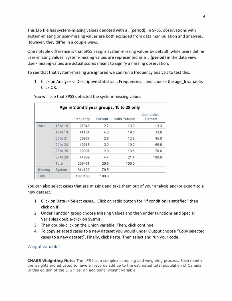
To see that that system-missing are ignored we can run a frequency analysis to test this.

1. Click on Analyze -> Descriptive statistics... Frequencies... and choose the age_6 variable.

Click OK.

You will see that SPSS detected the system-missing values

You can also select cases that are missing and take them out of your analysis and/or export to a

new dataset.

1. Click on Data -> Select cases... Click on radio button for “If condition is satisfied” then

click on If...

2. Under Function group choose Missing Values and then under Functions and Special

Variables double-click on Sysmis.

3. Then double-click on the Union variable. Then, click continue.

4. To copy selected cases to a new dataset you would under Output choose “Copy selected

cases to a new dataset”. Finally, click Paste. Then select and run your code.

Weight variables

CHASS Weighting Note: The LFS has a complex sampling and weighting process. Each month

the weights are adjusted to have all records add up to the estimated total population of Canada.

In this edition of the LFS files, an additional weight variable

5

fweighta has been created and is intended to be used when analyzing all 12 monthly

surveys of an LFS year at one time.

Each record contains a variable identifying the month. If you are doing an analysis on a monthly

basis and use only the records for that month then the weight variable will produce an estimate

for the total population. If you are using all records on the file (ie all 12 monthly surveys,

the weighted estimates (counts) using the 'fweight' variable provided by Statistics

Canada will be about 12 times what they should be. The computed 'fweighta' variable

consists of the 'fweight' variable divided by 12 to adjust for this.

Similarly, if you are using only 10 months worth of records then the estimate will be 10 times

what it should be and you must divide the resulting estimates (counts) by 10. This is not an

exact procedure and you may not end up with the same estimates as those released monthly by

Statistics Canada.

Let’s add the weight variable to the dataset so we can produce a population estimate for the

Canadian population using the cumulative CHASS file.

6

1. Run a frequency count for lfsstat (labour force status) and compare the numbers with

the weight on and the weight off. For fun add the fweight to see the grossly inflated

amount.

Select cases and using conditional expressions

You might also be interested in running some analyses only for a selected group of cases with certain

characteristics.

In this case, you will need to use the SPSS command called select cases.

1. To select cases, follow Data -> Select cases. Select If condition is satisfied.

7

2. Then click on If...

3. Write an expression where those living in Vancouver work for a firm that is more than 500

employees in size and whose occupational status is senior management

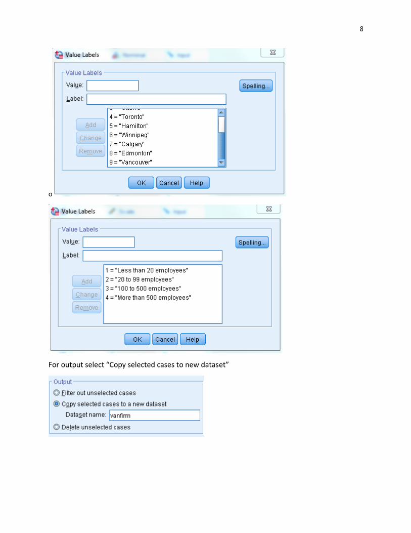
8

o

For output select “Copy selected cases to new dataset”

9

Click Paste and run the code in the Syntax editor.

Recode variables

Sometimes you will want to transform a variable by grouping its categories or values together.

For example, you may want to change a continuous variable into a categorical variable, or you

may want to merge the categories of a nominal variable. In SPSS, this type of transform is called

recoding.

Let’s consider you want to do a comparison of unemployment that looks at 15-29 years

compared to 30-44 years and 45-59 years.

We can see that the values of the age_12 includes 5-year age groups that could be aggregated

up.

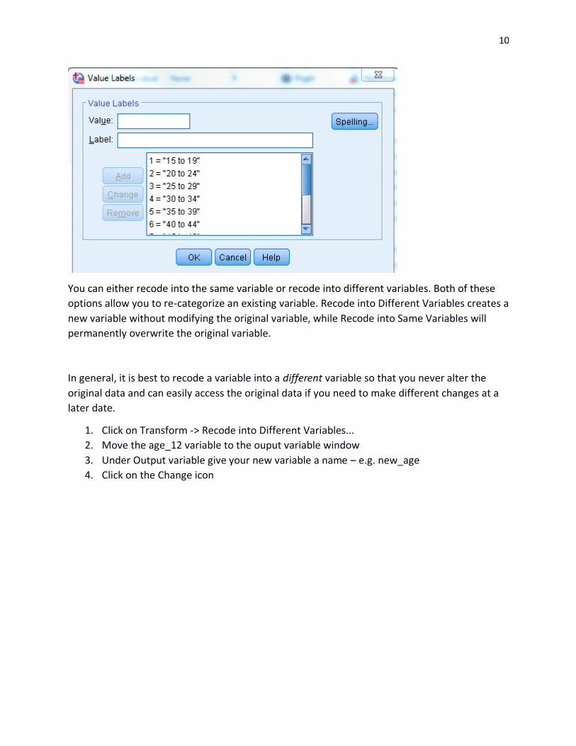
10

You can either recode into the same variable or recode into different variables. Both of these

options allow you to re-categorize an existing variable. Recode into Different Variables creates a

new variable without modifying the original variable, while Recode into Same Variables will

permanently overwrite the original variable.

In general, it is best to recode a variable into a different variable so that you never alter the

original data and can easily access the original data if you need to make different changes at a

later date.

1. Click on Transform -> Recode into Different Variables...

2. Move the age_12 variable to the ouput variable window

3. Under Output variable give your new variable a name – e.g. new_age

4. Click on the Change icon

11

5. Click on Old and New Values...

6. Under Old Value choose range and enter the old ranges you wish to aggregate into a

new value

7. Under new value specify a number for each new grouping and then click on Add

8. Repeat for each new grouping

9. Click Continue and then Paste and run your code in the Syntax editor window

10. Go to Data View to see your new_age variable appended to the end

11. Run a frequency count to see the new distribution for the new groupings

12

Calculating unemployment rate

By definition, unemployment rate refers to the percentage of the unemployed population over

the active population at a given point in time.

Unemployment rate is therefore calculated by dividing the number of unemployed people by

the number of people in the labour force.

The lfsstat variable counts both of these measures:

1. Click on Transform -> Recode into Different Variables...

2. Move lfsstat to Output Variable window

3. Give new variable a name (e.g. employed)

13

4. Click on Old and New Values...

5. Under Old Value -> Range put 1 - 2

6. Under New Value -> Value put 1

7. Click on Add

8. Then click Continue and paste and run your code in the Syntax Editor

9. Do the same thing for the unemployed value in lfsstat. In other words create another

new variable for unemployed

10. Click on Transform -> Recode into Different Variables...

11. Move lfsstat to Output window

12. Give new variable a name (e.g. unemployed)

13. This time under Old Value -> Value put 3

14. Under New Value -> Value put 2 (can be any integer)

14

15. Click Add and Continue and Paste and then run the code form the Syntax Editor

15. Go to Data View to see the two newly created variables

16. To calculate unemployment rate, run frequency counts for the two new variables and

then divided the unemployed SUM by employed at work SUM.

BONUS question – how would you calculate the unemployment rate for just the month of

January 2018?

Cross tabulations

Crosstabulation is used to display the common distribution of two variables. In addition, tests of

significance and measures of association may be used. In more detail, the values of one of the

variables are displayed in the columns of the table and those of the other variable will be

displayed in the rows. The cells that are formed by the intersection of columns and rows will

display the number of cases that have both the value in the respective column and that in the

respective row.

Let’s run a cross tabulation between the 9 major census metropolitan areas and labour force

status.

1. Go to Analyze -> Descriptive Statistics -> Crosstabs...

2. Put CMA in Row and lfsstat in Column

15

3. One important consideration is to be mindful of the difference between row and

column percentages.

4. Click on Cells... and choose column percentages.

16

5. Click Continue and Paste and then run your code from the Syntax Editor.

17