Introduction to Data Analysis. Multivariate Linear Regression.
53
Introduction to Data Analysis. Multivariate Linear Regression
-
Upload
linette-bates -
Category
Documents
-
view
234 -
download
1
Transcript of Introduction to Data Analysis. Multivariate Linear Regression.

Introduction to Data Analysis.
Multivariate Linear Regression
2
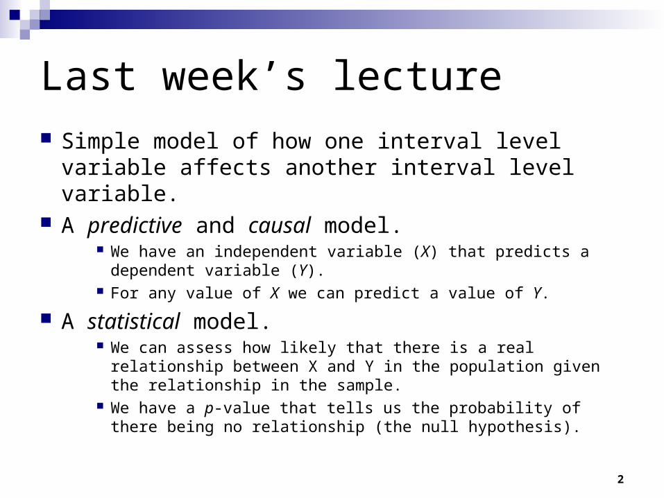
Last week’s lecture
Simple model of how one interval level variable affects another interval level variable.
A predictive and causal model. We have an independent variable (X) that predicts a dependent
variable (Y). For any value of X we can predict a value of Y.
A statistical model. We can assess how likely that there is a real relationship between
X and Y in the population given the relationship in the sample. We have a p-value that tells us the probability of there being no
relationship (the null hypothesis).
3
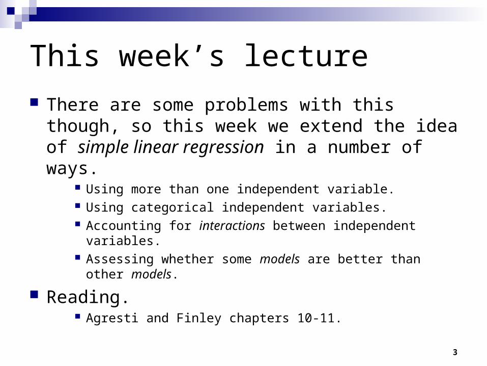
This week’s lecture
There are some problems with this though, so this week we extend the idea of simple linear regression in a number of ways.
Using more than one independent variable. Using categorical independent variables. Accounting for interactions between independent variables. Assessing whether some models are better than other models.
Reading. Agresti and Finley chapters 10-11.
4
Causation (1)
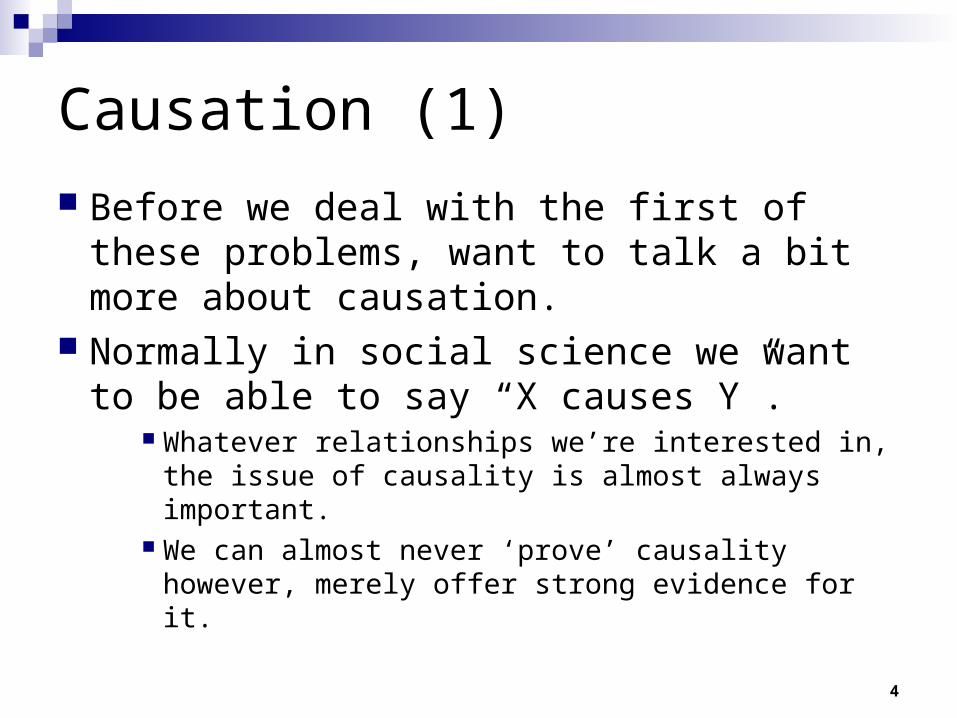
Before we deal with the first of these problems, want to talk a bit more about causation.
Normally in social science we want to be able to say “X causes Y”.
Whatever relationships we’re interested in, the issue of causality is almost always important.
We can almost never ‘prove’ causality however, merely offer strong evidence for it.
5
Causation (2)
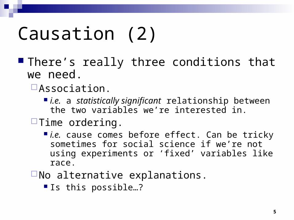
There’s really three conditions that we need.Association.
i.e. a statistically significant relationship between the two variables we’re interested in.
Time ordering. i.e. cause comes before effect. Can be tricky sometimes
for social science if we’re not using experiments or ‘fixed’ variables like race.
No alternative explanations. Is this possible…?
6
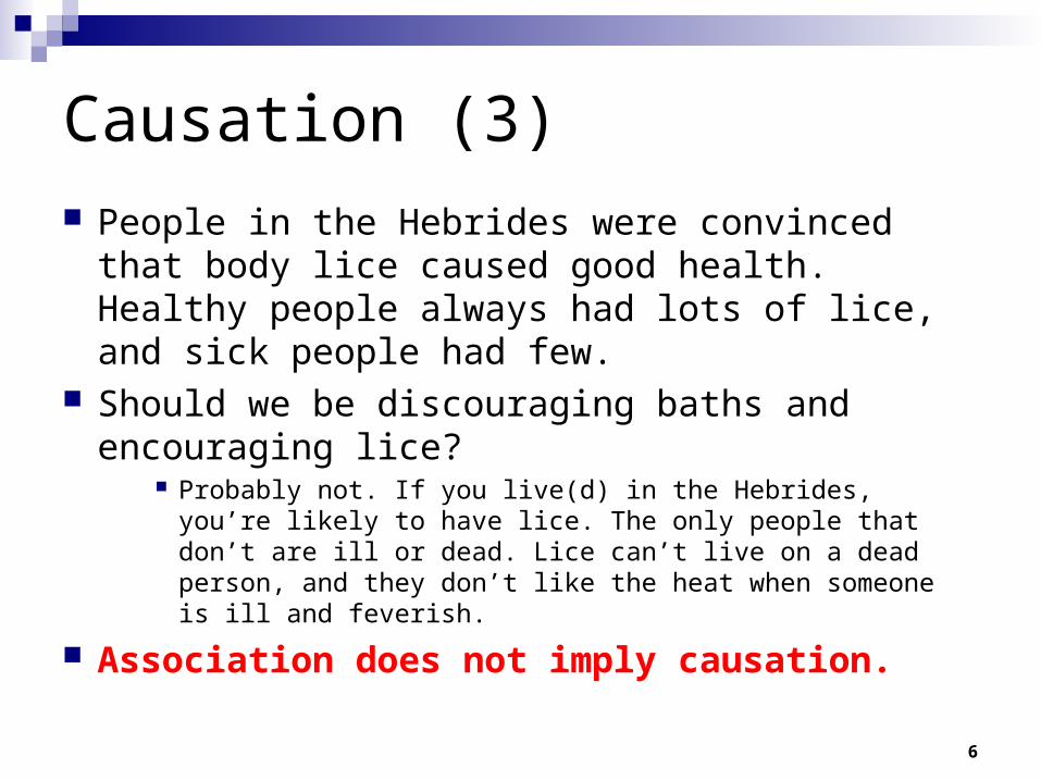
Causation (3)
People in the Hebrides were convinced that body lice caused good health. Healthy people always had lots of lice, and sick people had few.
Should we be discouraging baths and encouraging lice?
Probably not. If you live(d) in the Hebrides, you’re likely to have lice. The only people that don’t are ill or dead. Lice can’t live on a dead person, and they don’t like the heat when someone is ill and feverish.
Association does not imply causation.

7
The ideal Daily Mail headline… Do booze fuelled yobs increase your mortgage?
8
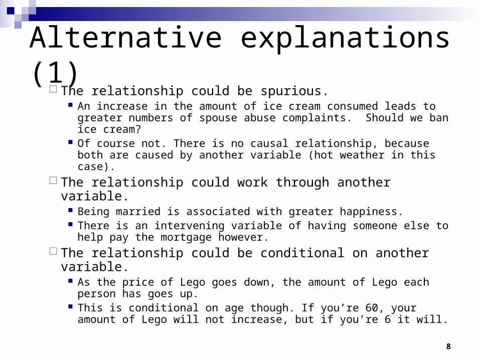
Alternative explanations (1) The relationship could be spurious.
An increase in the amount of ice cream consumed leads to greater numbers of spouse abuse complaints. Should we ban ice cream?
Of course not. There is no causal relationship, because both are caused by another variable (hot weather in this case).
The relationship could work through another variable. Being married is associated with greater happiness. There is an intervening variable of having someone else to help
pay the mortgage however. The relationship could be conditional on another variable.
As the price of Lego goes down, the amount of Lego each person has goes up.
This is conditional on age though. If you’re 60, your amount of Lego will not increase, but if you’re 6 it will.
9
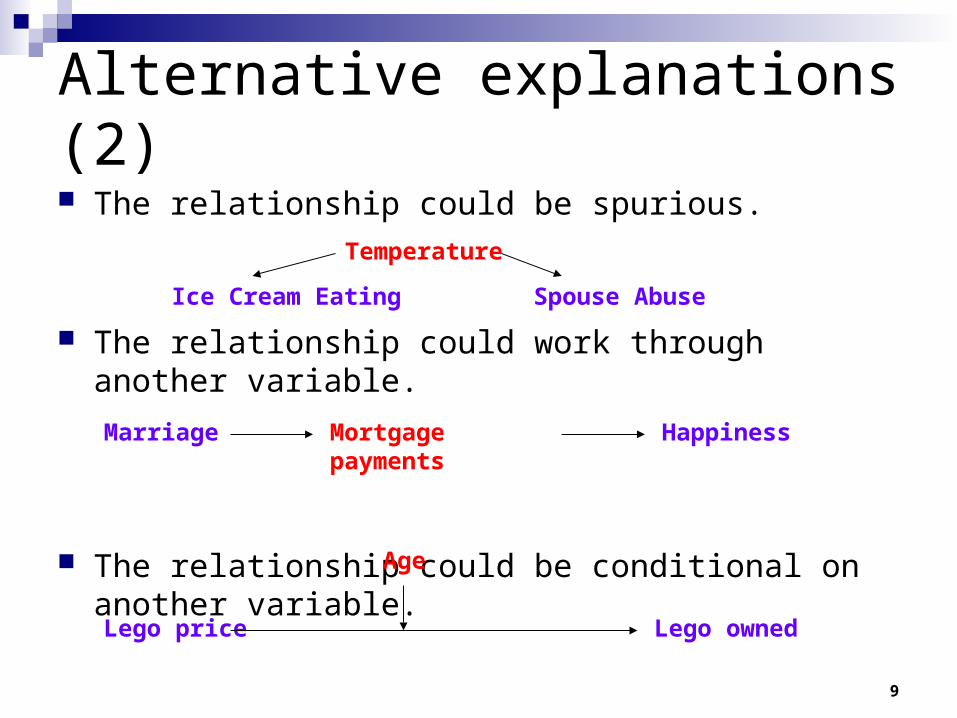
Alternative explanations (2) The relationship could be spurious.
The relationship could work through another variable.
The relationship could be conditional on another variable.
Temperature
Spouse AbuseIce Cream Eating
Mortgage payments HappinessMarriage
Age
Lego ownedLego price
10
Experiments and causality
We could virtually eliminate these problems if we used experiments.
Experiments mean that we can change the variable we are interested in and see how people respond.
Becoming more popular in social science.
Unfortunately we are normally reliant on observational data.
Therefore we want to try and control for alternative explanations.
The best way of doing this is to use multiple regression.
11
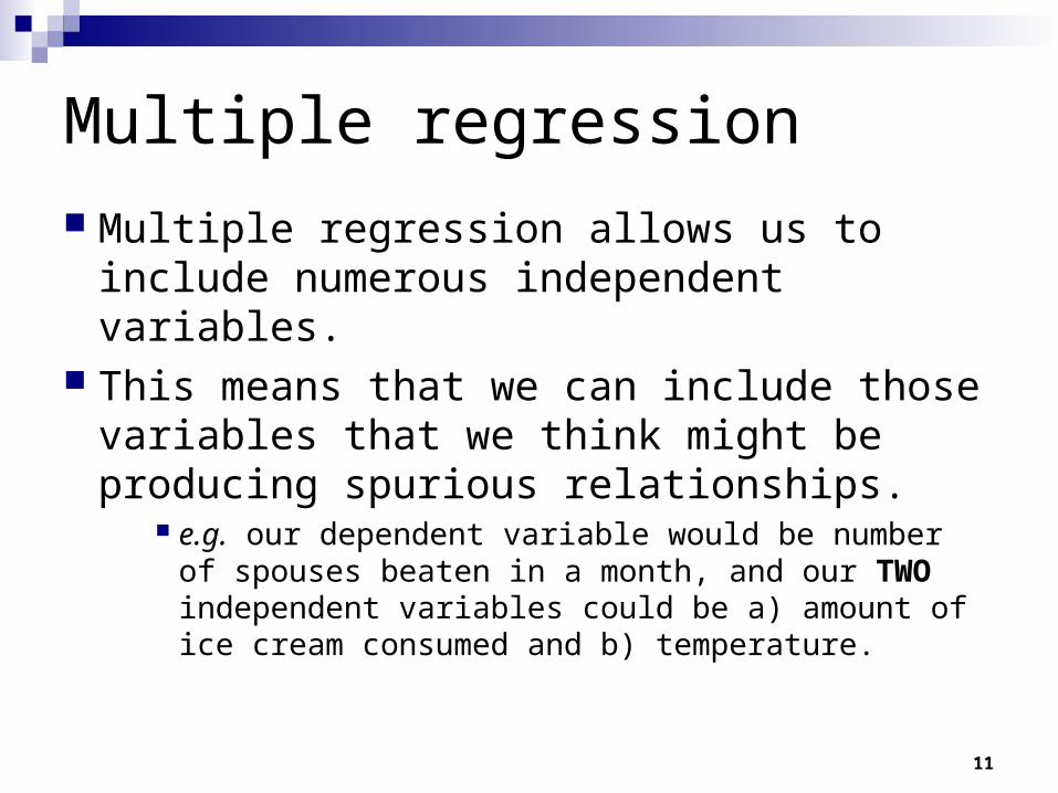
Multiple regression
Multiple regression allows us to include numerous independent variables.
This means that we can include those variables that we think might be producing spurious relationships.
e.g. our dependent variable would be number of spouses beaten in a month, and our TWO independent variables could be a) amount of ice cream consumed and b) temperature.
12
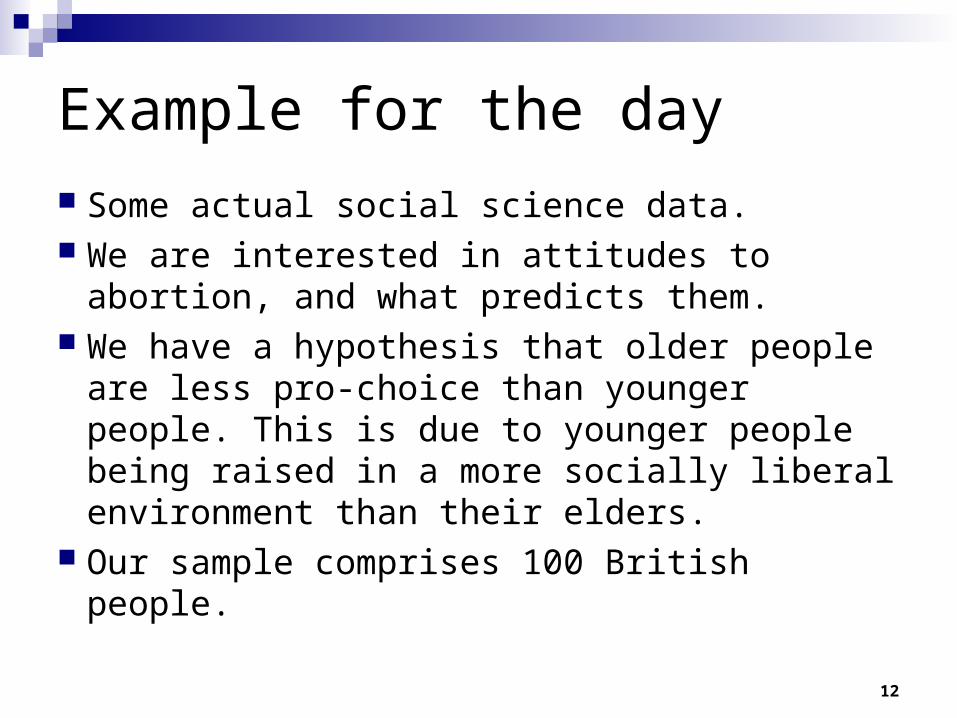
Example for the day
Some actual social science data. We are interested in attitudes to abortion, and
what predicts them. We have a hypothesis that older people are
less pro-choice than younger people. This is due to younger people being raised in a more socially liberal environment than their elders.
Our sample comprises 100 British people.
13
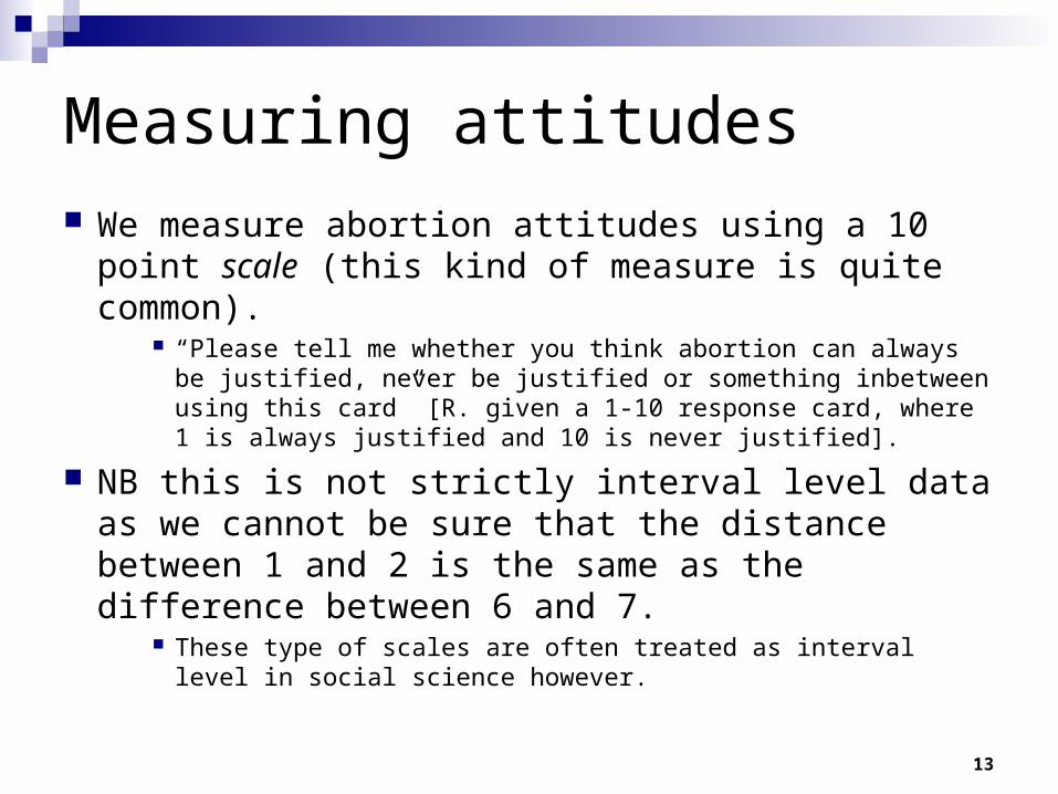
Measuring attitudes
We measure abortion attitudes using a 10 point scale (this kind of measure is quite common).
“Please tell me whether you think abortion can always be justified, never be justified or something inbetween using this card” [R. given a 1-10 response card, where 1 is always justified and 10 is never justified].
NB this is not strictly interval level data as we cannot be sure that the distance between 1 and 2 is the same as the difference between 6 and 7.
These type of scales are often treated as interval level in social science however.
14
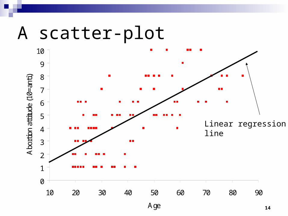
A scatter-plot
0
1
2
3
4
5
6
7
8
9
10
10 20 30 40 50 60 70 80 90
Age
Abo
rtio
n at
titud
e (1
0=an
ti)
Linear regressionline
15
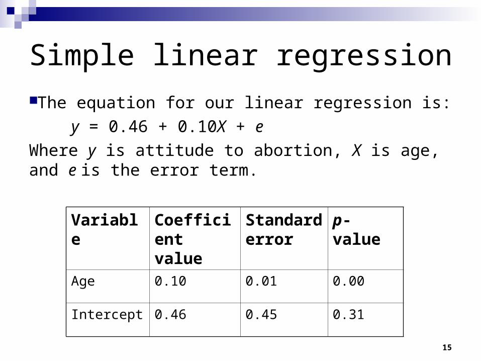
Simple linear regression
The equation for our linear regression is:
y = 0.46 + 0.10X + e
Where y is attitude to abortion, X is age, and e is the error term.
Variable Coefficient value
Standard error
p-value
Age 0.10 0.01 0.00
Intercept 0.46 0.45 0.31
16
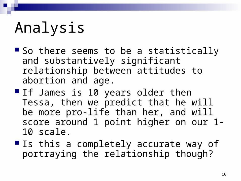
Analysis
So there seems to be a statistically and substantively significant relationship between attitudes to abortion and age.
If James is 10 years older then Tessa, then we predict that he will be more pro-life than her, and will score around 1 point higher on our 1-10 scale.
Is this a completely accurate way of portraying the relationship though?
17
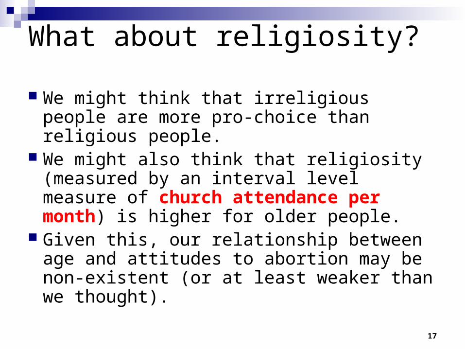
What about religiosity?
We might think that irreligious people are more pro-choice than religious people.
We might also think that religiosity (measured by an interval level measure of church attendance per month) is higher for older people.
Given this, our relationship between age and attitudes to abortion may be non-existent (or at least weaker than we thought).
18
Some data
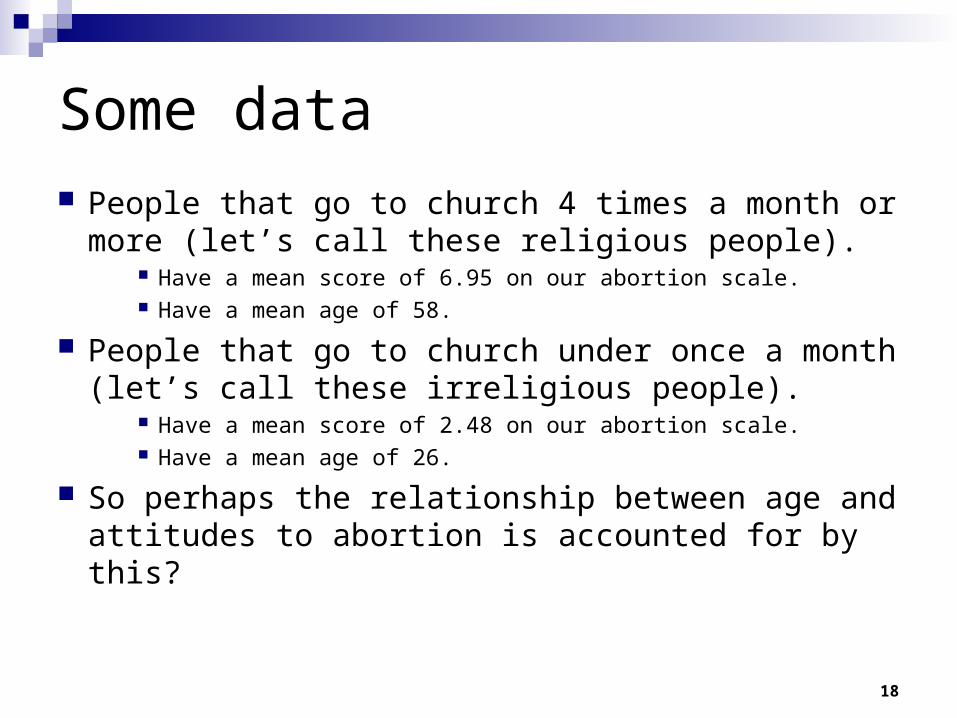
People that go to church 4 times a month or more (let’s call these religious people).
Have a mean score of 6.95 on our abortion scale. Have a mean age of 58.
People that go to church under once a month (let’s call these irreligious people).
Have a mean score of 2.48 on our abortion scale. Have a mean age of 26.
So perhaps the relationship between age and attitudes to abortion is accounted for by this?
19
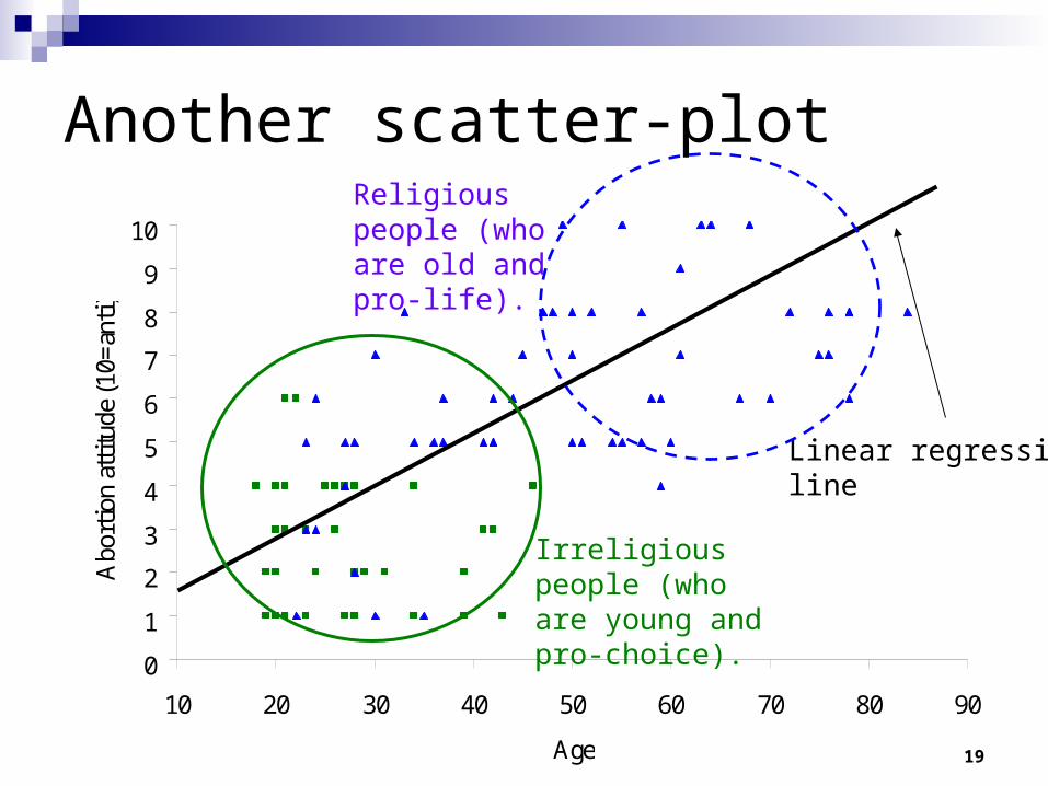
Another scatter-plot
0
1
2
3
4
5
6
7
8
9
10
10 20 30 40 50 60 70 80 90
Age
Abo
rtio
n at
titu
de (
10=
anti
)
Linear regressionline
Irreligious people (who are young and pro-choice).
Religious people (who are old and pro-life).
20
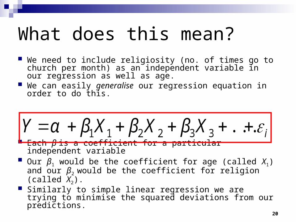
What does this mean? We need to include religiosity (no. of times go to church per
month) as an independent variable in our regression as well as age.
We can easily generalise our regression equation in order to do this.
Each β is a coefficient for a particular independent variable Our β1 would be the coefficient for age (called X1) and our β2
would be the coefficient for religion (called X2). Similarly to simple linear regression we are trying to minimise
the squared deviations from our predictions.
21
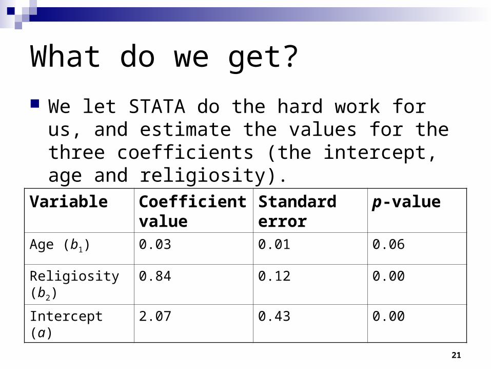
What do we get?
We let STATA do the hard work for us, and estimate the values for the three coefficients (the intercept, age and religiosity).
Variable Coefficient value
Standard error
p-value
Age (b1) 0.03 0.01 0.06
Religiosity (b2) 0.84 0.12 0.00
Intercept (a) 2.07 0.43 0.00
22
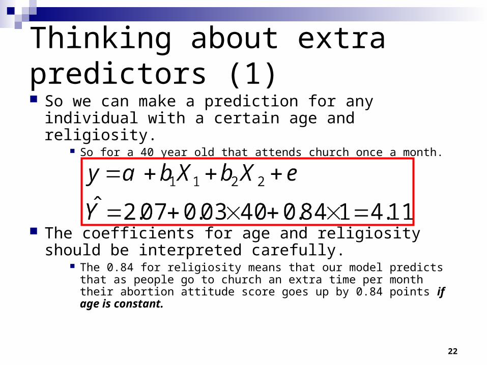
Thinking about extra predictors (1) So we can make a prediction for any individual with
a certain age and religiosity. So for a 40 year old that attends church once a month.
The coefficients for age and religiosity should be interpreted carefully.
The 0.84 for religiosity means that our model predicts that as people go to church an extra time per month their abortion attitude score goes up by 0.84 points if age is constant.
23
Thinking about extra predictors (2)
Thus, the best way of thinking about regression with more than one independent variable is to imagine a separate regression line for age at each value of religiosity, and vice versa.
The effect of age is the slope of these parallel lines, controlling for the effect of religiosity.
24
0
1
2
3
4
5
6
7
8
9
10
10 20 30 40 50 60 70 80 90
Age
Abo
rtio
n at
titu
de (
10=
anti
)
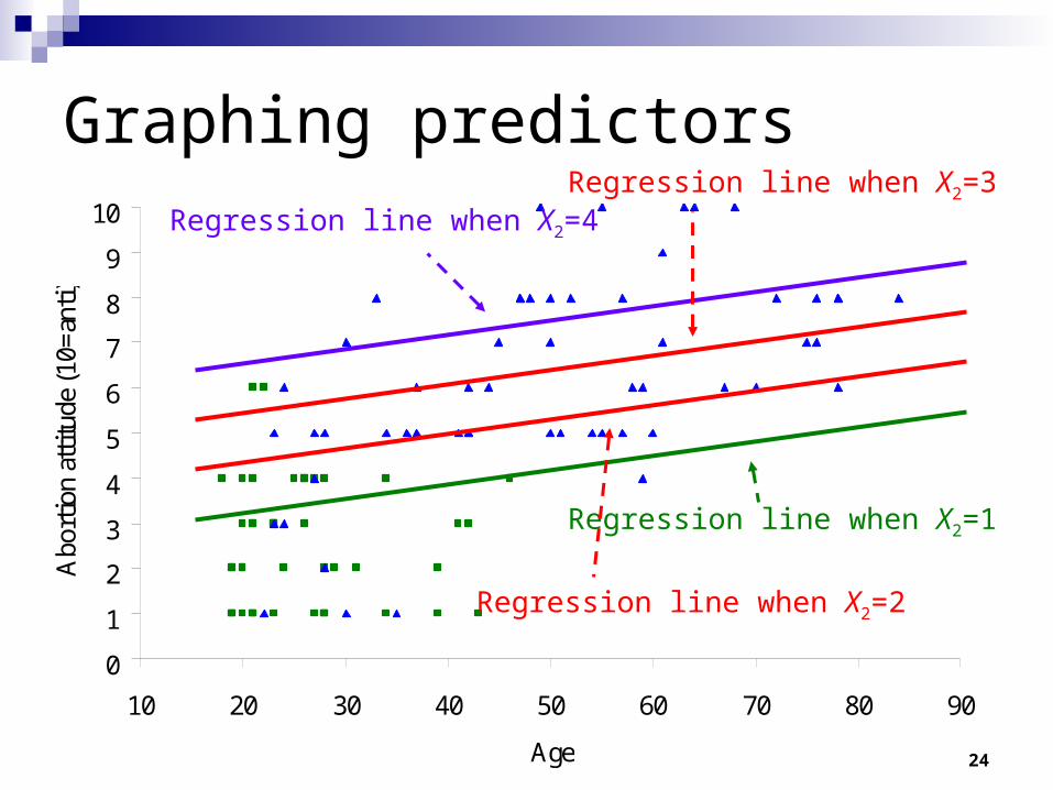
Graphing predictors
Regression line when X2=1
Regression line when X2=4
Regression line when X2=2
Regression line when X2=3
25
Multiple regression summary
Our example only has two predictors, but we can have any number of independent variables.
Thus, multiple regression is a really useful extension of simple linear regression.
Multiple regression is a way of reducing spurious relationships between variables by including the real cause.
Multiple regression is also a way of testing whether a relationship is actually working through another variable (as it appears to be in our example).
26
Comparing groups (1)
The independent variables we’ve been using are all interval level (age, number of times attended church etc.).
A lot of social science variables that we are interested in are actually categorical though, how do we include these?
We create ‘dummy’ variables (i.e. 0/1 variables which can be included in the regression).
27
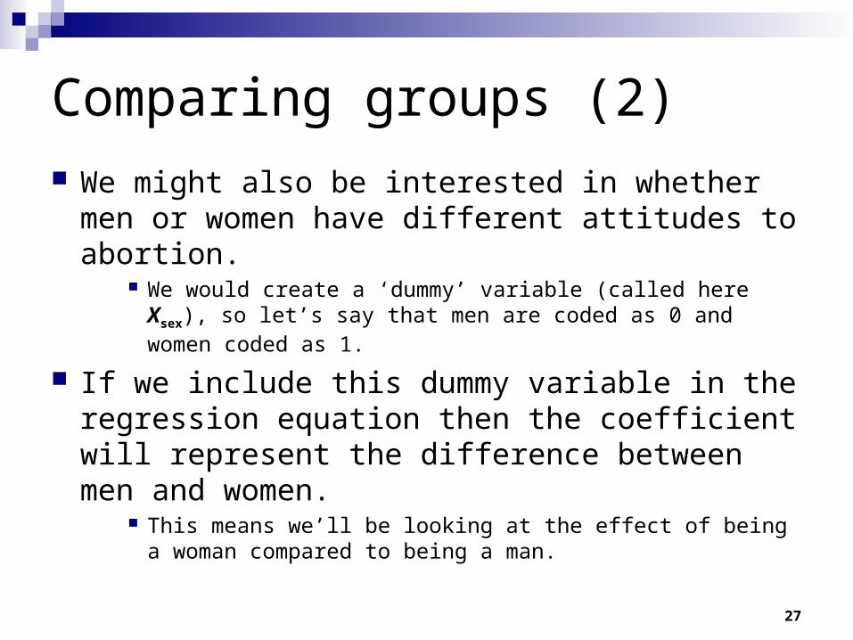
Comparing groups (2)
We might also be interested in whether men or women have different attitudes to abortion.
We would create a ‘dummy’ variable (called here Xsex), so let’s say that men are coded as 0 and women coded as 1.
If we include this dummy variable in the regression equation then the coefficient will represent the difference between men and women.
This means we’ll be looking at the effect of being a woman compared to being a man.
28
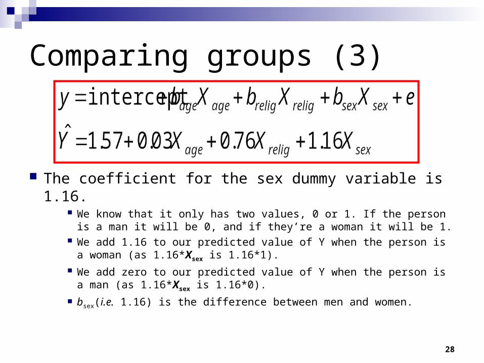
Comparing groups (3)
The coefficient for the sex dummy variable is 1.16. We know that it only has two values, 0 or 1. If the person is a man
it will be 0, and if they’re a woman it will be 1. We add 1.16 to our predicted value of Y when the person is a
woman (as 1.16*Xsex is 1.16*1). We add zero to our predicted value of Y when the person is a man
(as 1.16*Xsex is 1.16*0).
bsex(i.e. 1.16) is the difference between men and women.
29
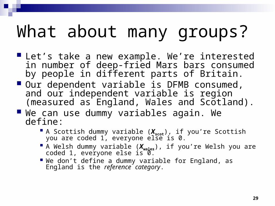
What about many groups? Let’s take a new example. We’re interested in number
of deep-fried Mars bars consumed by people in different parts of Britain.
Our dependent variable is DFMB consumed, and our independent variable is region (measured as England, Wales and Scotland).
We can use dummy variables again. We define: A Scottish dummy variable (Xscot), if you’re Scottish you are coded
1, everyone else is 0. A Welsh dummy variable (Xwales), if you’re Welsh you are coded 1,
everyone else is 0. We don’t define a dummy variable for England, as England is the
reference category.
30
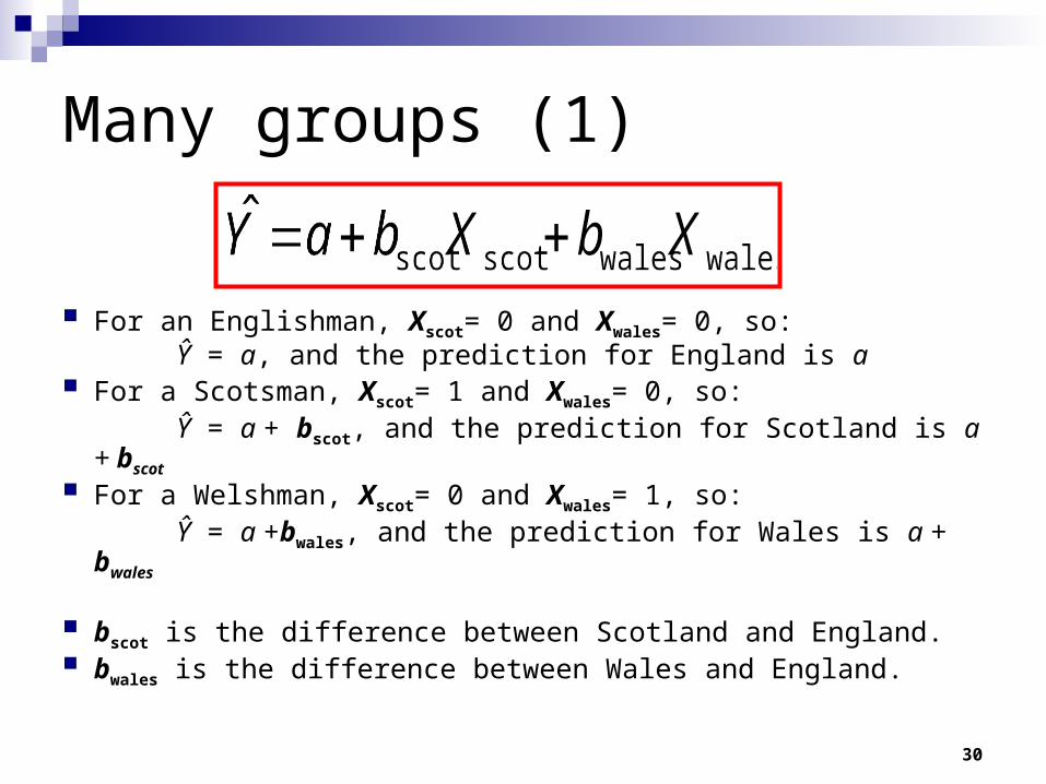
Many groups (1)
For an Englishman, Xscot= 0 and Xwales= 0, so: Ŷ = a, and the prediction for England is a For a Scotsman, Xscot= 1 and Xwales= 0, so: Ŷ = a + bscot, and the prediction for Scotland is a + bscot
For a Welshman, Xscot= 0 and Xwales= 1, so: Ŷ = a +bwales, and the prediction for Wales is a + bwales
bscot is the difference between Scotland and England. bwales is the difference between Wales and England.
31
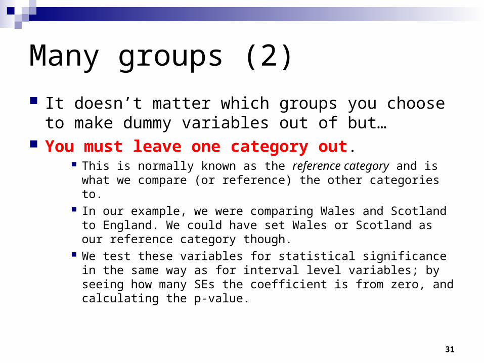
Many groups (2)
It doesn’t matter which groups you choose to make dummy variables out of but…
You must leave one category out. This is normally known as the reference category and is what we
compare (or reference) the other categories to. In our example, we were comparing Wales and Scotland to
England. We could have set Wales or Scotland as our reference category though.
We test these variables for statistical significance in the same way as for interval level variables; by seeing how many SEs the coefficient is from zero, and calculating the p-value.
32
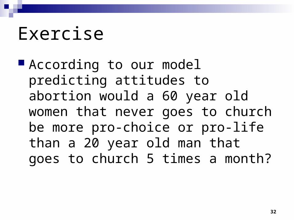
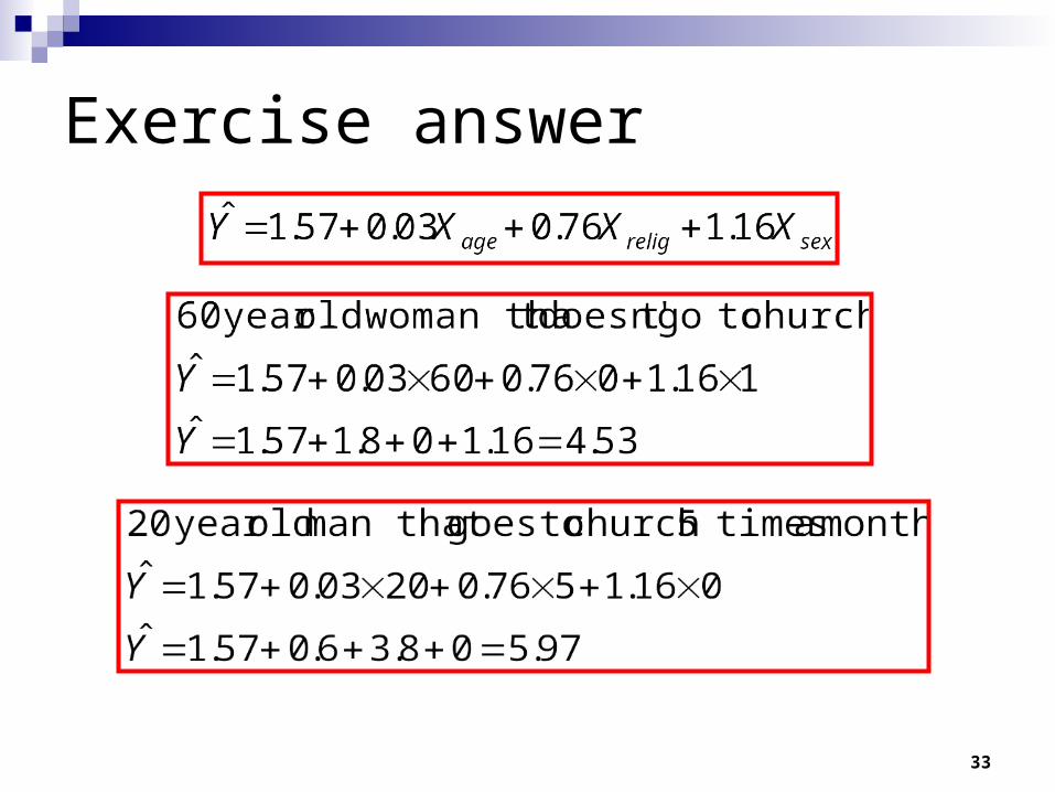
Exercise
According to our model predicting attitudes to abortion would a 60 year old women that never goes to church be more pro-choice or pro-life than a 20 year old man that goes to church 5 times a month?
33
Exercise answer
34
‘Interactions’
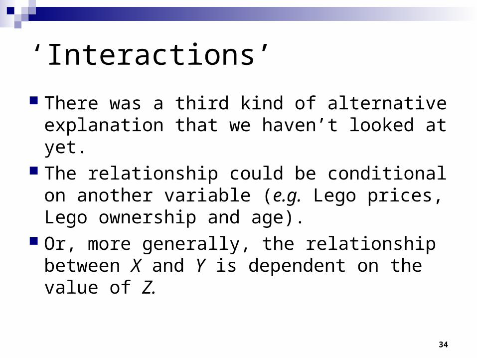
There was a third kind of alternative explanation that we haven’t looked at yet.
The relationship could be conditional on another variable (e.g. Lego prices, Lego ownership and age).
Or, more generally, the relationship between X and Y is dependent on the value of Z.
35
Another example of the day
We might think that the longer you are married the more that you nag your spouse.
Our dependent variable is the amount of nagging that an individual does, in minutes per day.
Our independent variable is years of marriage. The population of interest is all married people. We have a sample of 50 married people.
First step, let’s look at the data.
36
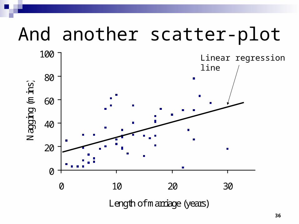
And another scatter-plot
0
20
40
60
80
100
0 10 20 30
Length of marriage (years)
Nag
ging
(m
ins)
Linear regressionline
37
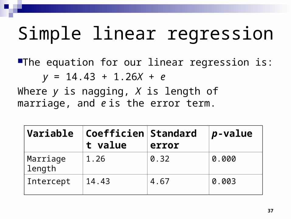
Simple linear regression
The equation for our linear regression is:
y = 14.43 + 1.26X + e
Where y is nagging, X is length of marriage, and e is the error term.
Variable Coefficient value
Standard error
p-value
Marriage length 1.26 0.32 0.000
Intercept 14.43 4.67 0.003
38
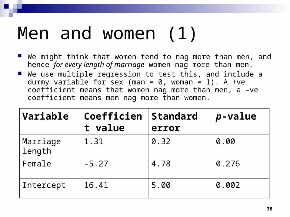
Men and women (1) We might think that women tend to nag more than men, and hence for
every length of marriage women nag more than men. We use multiple regression to test this, and include a dummy variable for
sex (man = 0, woman = 1). A +ve coefficient means that women nag more than men, a –ve coefficient means men nag more than women.
Variable Coefficient value
Standard error
p-value
Marriage length 1.31 0.32 0.00
Female -5.27 4.78 0.276
Intercept 16.41 5.00 0.002
39
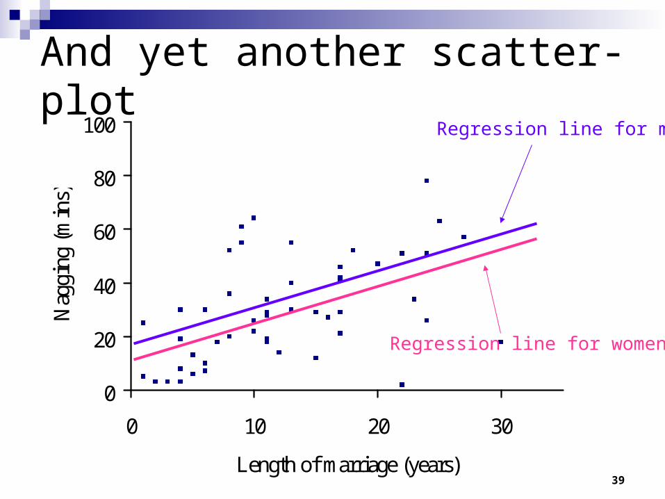
And yet another scatter-plot
0
20
40
60
80
100
0 10 20 30
Length of marriage (years)
Nag
ging
(m
ins)
Regression line for men
Regression line for women
40
Men and women (2)
There does not appear to be a statistically significant difference between men and women.
Perhaps the difference between men and women in how much they nag differs by length of marriage though?
This is what we call an interaction effect, for different levels of a variable Z the effect of X on Y is different.
Let’s examine the data again.
41
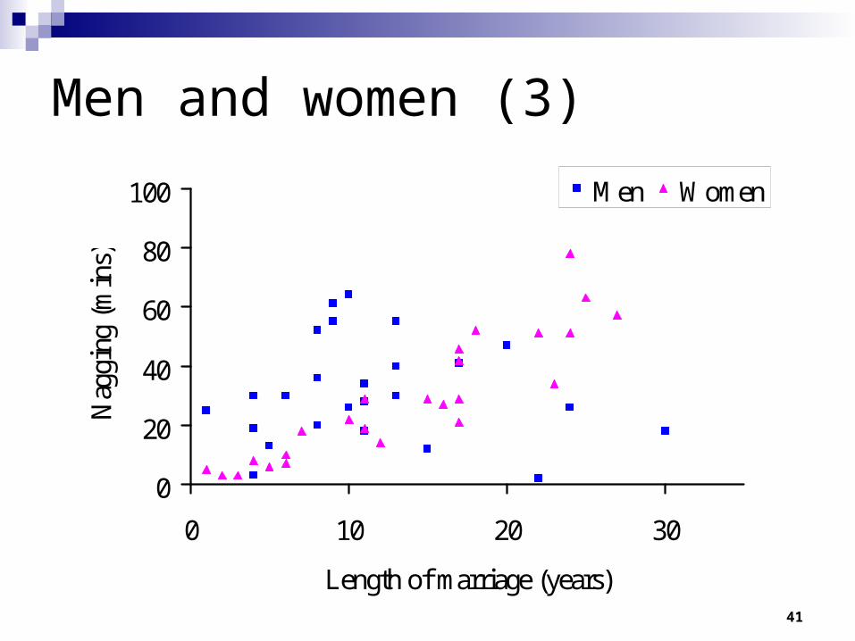
Men and women (3)
0
20
40
60
80
100
0 10 20 30
Length of marriage (years)
Nag
ging
(m
ins)
Men Women
42
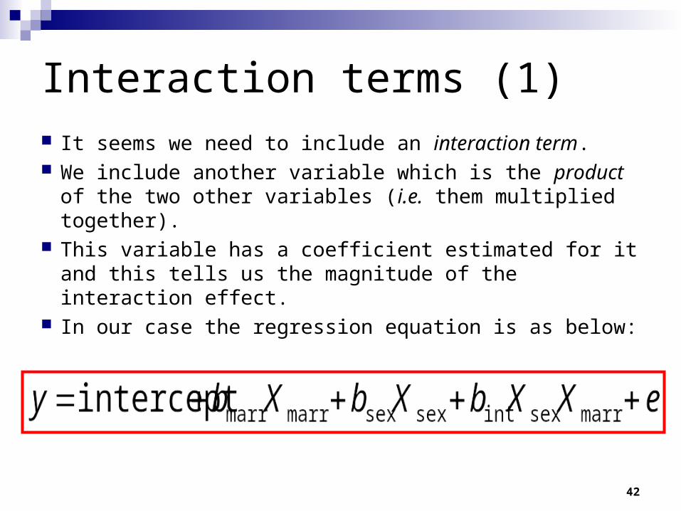
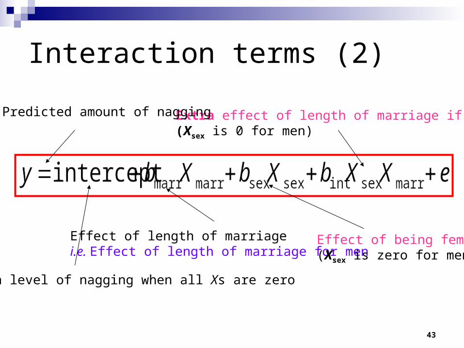
Interaction terms (1)
It seems we need to include an interaction term. We include another variable which is the product of
the two other variables (i.e. them multiplied together).
This variable has a coefficient estimated for it and this tells us the magnitude of the interaction effect.
In our case the regression equation is as below:
43
Interaction terms (2)
Extra effect of length of marriage if female(Xsex is 0 for men)
Effect of length of marriagei.e. Effect of length of marriage for men
Predicted amount of nagging
Effect of being female(Xsex is zero for men)
Mean level of nagging when all Xs are zero
44
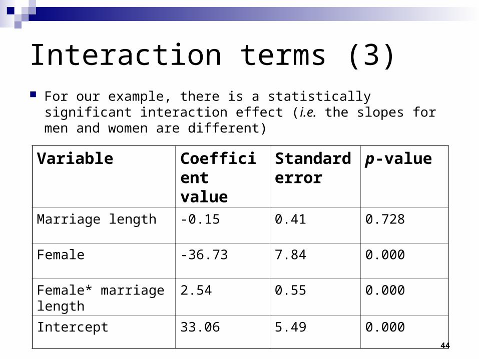
Interaction terms (3) For our example, there is a statistically significant interaction
effect (i.e. the slopes for men and women are different)
Variable Coefficient value
Standard error
p-value
Marriage length -0.15 0.41 0.728
Female -36.73 7.84 0.000
Female* marriage length 2.54 0.55 0.000
Intercept 33.06 5.49 0.000
45
0
20
40
60
80
100
0 10 20 30
Length of marriage (years)
Nag
ging
(m
ins)
Men Women
Interaction terms (4)
Women
Men
46
Final word on interactions
More generally we can ‘interact’ variables of all sorts.
With our dummy variable*length of marriage, we generate a separate slope for men and women.
If we were interacting two interval level variables, say age and religiosity, then it is best to think of generating a particular slope for the relationship between age and the dependent variable for each different value of religiosity.
e.g. we want to say something like: at high levels of religiosity age has a large effect, but at low levels of religiosity age has a small effect.
47
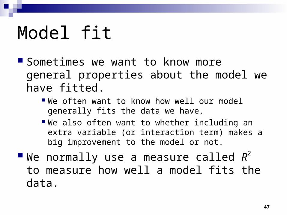
Model fit
Sometimes we want to know more general properties about the model we have fitted.
We often want to know how well our model generally fits the data we have.
We also often want to whether including an extra variable (or interaction term) makes a big improvement to the model or not.
We normally use a measure called R2 to measure how well a model fits the data.
48
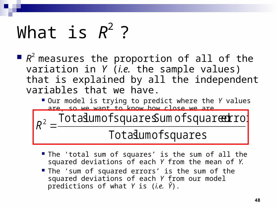
What is R2 ? R2 measures the proportion of all of the variation in Y
(i.e. the sample values) that is explained by all the independent variables that we have.
Our model is trying to predict where the Y values are, so we want to know how close we are.
The ‘total sum of squares’ is the sum of all the squared deviations of each Y from the mean of Y.
The ‘sum of squared errors’ is the sum of the squared deviations of each Y from our model predictions of what Y is (i.e. Ŷ).
49
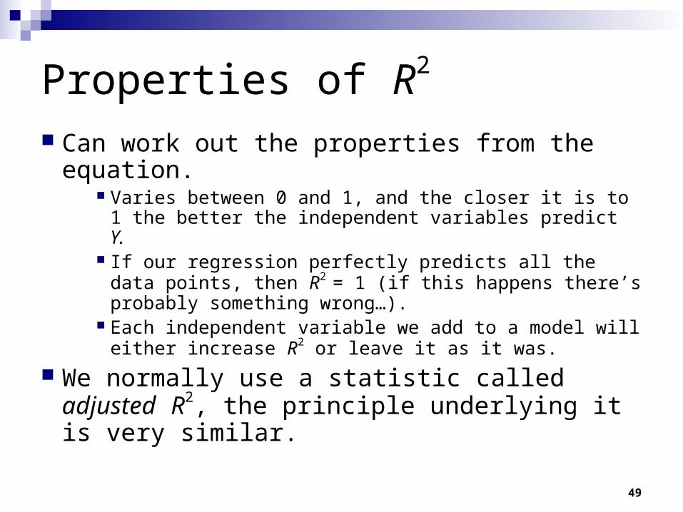
Properties of R2
Can work out the properties from the equation. Varies between 0 and 1, and the closer it is to 1 the
better the independent variables predict Y. If our regression perfectly predicts all the data points,
then R2 = 1 (if this happens there’s probably something wrong…).
Each independent variable we add to a model will either increase R2 or leave it as it was.
We normally use a statistic called adjusted R2, the principle underlying it is very similar.
50
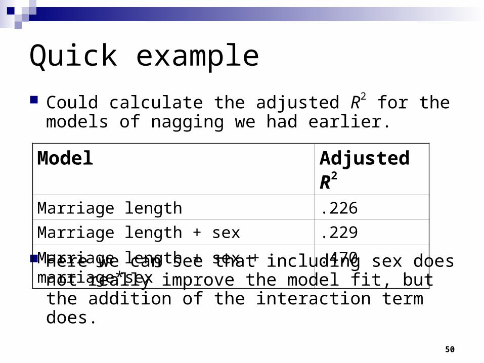
Quick example Could calculate the adjusted R2 for the models of
nagging we had earlier.
Here we can see that including sex does not really improve the model fit, but the addition of the interaction term does.
Model Adjusted R2
Marriage length .226
Marriage length + sex .229
Marriage length + sex + marriage*sex .470
51
When’s an increase a real increase?
We can test whether increases are statistically significant using something called a F-test
This is based on a distribution called the F-distribution.
This test tells us whether we can reject the null hypothesis that the increase in model fit is zero.
In our example, we cannot reject the H0 that the addition of sex to the model does not increase model fit.
We can reject the H0 that the addition of sex*marriage length to the model does not increase model fit.
52
Over-interpreting R2
R2 can be a useful measure of model ‘performance’, but it is not what we are often interested in.
Many social science models have low R2 values, but this doesn’t mean that they are useless. Rather it just means that there is a lot of variation not explained by our independent variables.
We still might be interested in whether there is a relationship between X and Y though.
High R2 values don’t automatically make your model a good model.
I could predict attitudes to having a European army using attitudes to the Euro. The R2 would be high, but it is unclear what the model is showing…
53
Problems with all this…
We’ve managed to get beyond several problems with simple linear regression, but…
How do we know when the assumptions (for example linearity) that underlie regression models are met?
Use plots of the ‘residuals’ (the differences between the actual observations and our predictions) to try and work out when different assumptions are not met.
More generally, how do we go about specifying models?
All to be dealt with next week.