Introduction to Credibility CAS Seminar on Ratemaking Las Vegas, Nevada March 12-13, 2001
32
Introduction to Credibility CAS Seminar on Ratemaking Las Vegas, Nevada March 12-13, 2001
-
Upload
tamanna-darshan -
Category
Documents
-
view
32 -
download
1
description
Introduction to Credibility CAS Seminar on Ratemaking Las Vegas, Nevada March 12-13, 2001. Purpose. Today’s session is designed to encompass: Credibility in the context of ratemaking Classical and Bühlmann models Review of variables affecting credibility Formulas - PowerPoint PPT Presentation
Transcript of Introduction to Credibility CAS Seminar on Ratemaking Las Vegas, Nevada March 12-13, 2001

Introduction to Credibility
CAS Seminar on RatemakingLas Vegas, NevadaMarch 12-13, 2001

Purpose
Today’s session is designed to encompass:
Credibility in the context of ratemaking Classical and Bühlmann models Review of variables affecting credibility Formulas Practical techniques for applying Methods for increasing credibility

Outline
Background Definition Rationale History
Methods, examples, and considerations Limited fluctuation methods Greatest accuracy methods
Bibliography

Background

Background
Definition
Common vernacular (Webster): “Credibility:” the state or quality of being credible “Credible:” believable So, “the quality of being believable” Implies you are either credible or you are not
In actuarial circles: Credibility is “a measure of the credence that…should be
attached to a particular body of experience”
-- L.H. Longley-Cook Refers to the degree of believability; a relative concept
Background
Rationale
Why do we need “credibility” anyway?
P&C insurance costs, namely losses, are inherently stochastic
Observation of a result (data) yields only an estimate of the “truth”
How much can we believe our data?
Consider an example...

Background
Simple example

Background
History
The CAS was founded in 1914, in part to help make rates for a new line of insurance -- Work Comp
Early pioneers: Mowbray -- how many trials/results need to be observed
before I can believe my data? Albert Whitney -- focus was on combining existing estimates
and new data to derive new estimates
New Rate = Credibility*Observed Data + (1-Credibility)*Old Rate
Perryman (1932) -- how credible is my data if I have less than required for full credibility?
Bayesian views resurrected in the 40’s, 50’s, and 60’s

Background
Methods
“Frequentist”
Bayesian
Greatest Accuracy
LimitedFluctuation
Limit the effect that random fluctuations in the data can have on an estimate
Make estimation errors as small as possible
“Least Squares Credibility”“Empirical Bayesian Credibility”
Bühlmann CredibilityBühlmann-Straub Credibility
“Classical credibility”

Limited Fluctuation Credibility

Limited Fluctuation Credibility
Description
“A dependable [estimate] is one for which the probability is high, that it does not differ from the [truth] by more than an arbitrary limit.”
-- Mowbray
How much data is needed for an estimate so that the credibility, Z, reflects a probability, P, of being within a tolerance, k%, of the true value?

= (1-Z)*E1 + ZE[T] + Z*(T - E[T])
Limited Fluctuation Credibility
Derivation
E2 = Z*T + (1-Z)*E1
Add and subtract
ZE[T]
regroup
Stability Truth Random Error
New Estimate = (Credibility)(Data) + (1- Credibility)(Previous Estimate)
= Z*T + ZE[T] - ZE[T] + (1-Z)*E1
Limited Fluctuation Credibility
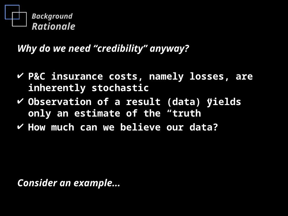
Mathematical formula for Z
Pr{Z(T-E[T]) < kE[T]} = P
-or- Pr{T < E[T] + kE[T]/Z} = P
E[T] + kE[T]/Z looks like a formula for a percentile:
E[T] + zpVar[T]1/2
-so- kE[T]/Z = zpVar[T]1/2
Z = kE[T]/zpVar[T]1/2

N = (zp/k)2
Limited Fluctuation Credibility
Mathematical formula for Z (continued)
If we assume That we are dealing with an insurance process that has Poisson
frequency, and Severity is constant or severity doesn’t matter
Then E[T] = number of claims (N), and E[T] = Var[T], so:
Solving for N (# of claims for full credibility, i.e., Z=1):
Z = kE[T]/zpVar[T]1/2 becomes:
Z = kE[T]1/2 /zp = kN1/2 /zp

Limited Fluctuation Credibility
Standards for full credibility
k
P 2.5% 5% 7.5% 10%
90% 4,326 1,082 481 291
95% 6,147 1,537 683 584
99% 10,623 2,656 1,180 664
Claim counts required for full credibility based on the previous derivation:

N = (zp/k)2{Var[N]/E[N] + Var[S]/E[S]}
Limited Fluctuation Credibility
Mathematical formula for Z II
Relaxing the assumption that severity doesn’t matter, let T = aggregate losses = (frequency)(severity) then E[T] = E[N]E[S] and Var[T] = E[N]Var[S] + E[S]2Var[N]
Plugging these values into the formula
Z = kE[T]/zpVar[T]1/2
and solving for N (@ Z=1):

Limited Fluctuation Credibility
Partial credibility
Given a full credibility standard, Nfull, what is the partial credibility of a number N < Nfull?
The square root rule says:
Z = (N/ Nfull)1/2
For example, let Nfull = 1,082, and say we have 500 claims. Z = (500/1082)1/2 = 68%

Limited Fluctuation Credibility
Partial credibility (continued)
20%30%40%50%60%70%80%90%
100%
100
300
500
700
900
1100
Number of Claims
Cre
dib
ilit
y
683
1,082
Full credibility standards:

Limited Fluctuation Credibility
Increasing credibility
Per the formula,
Z = (N/ Nfull)1/2 = [N/(zp/k)2]1/2 =
kN1/2/zp
Credibility, Z, can be increased by: Increasing N = get more data increasing k = accept a greater margin of error decrease zp = concede to a smaller P = be less certain
Limited Fluctuation Credibility
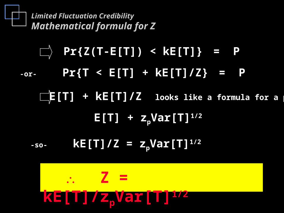
Weaknesses
The strength of limited fluctuation credibility is its simplicity, therefore its general acceptance and use. But it has weaknesses…
Establishing a full credibility standard requires arbitrary assumptions regarding P and k,
Typical use of the formula based on the Poisson model is inappropriate for most applications
Partial credibility formula -- the square root rule -- only holds for a normal approximation of the underlying distribution of the data. Insurance data tends to be skewed.
Treats credibility as an intrinsic property of the data.

Limited Fluctuation Credibility
Example
Calculate the expected loss ratios as part of an auto rate review for a given state.
Data:
Loss Ratio Claims
1995 67% 5351996 77% 6161997 79% 6341998 77% 6151999 86% 686 Credibility at: Weighted Indicated
1,082 5,410 Loss Ratio Rate Change3 year 81% 1,935 100% 60% 78.6% 4.8%5 year 77% 3,086 100% 75% 76.5% 2.0%
E.g., 81%(.60) + 75%(1-.60)
E.g., 76.5%/75% -1

Greatest Accuracy Credibility

Find the credibility weight, Z, that minimizes the sum of squared errors about the truth
For illustration, let Lij = loss ratio for territory i in year j; L.. is the grand mean
Lat = loss ratio for territory “a” at some future time “t”
Find Z that minimizes
E{Lat - [ZLa. + (1-Z)L..]}2
Z takes the form
Z = n/(n+k)
Greatest Accuracy Credibility
Derivation

k takes the form
k = s2/t2
where s2 = average variance of the territories over time, called the
expected value of process variance (EVPV) t2 = variance across the territory means, called the variance
of hypothetical means (VHM)
The greatest accuracy or least squares credibility result is more intuitively appealing. It is a relative concept It is based on relative variances or volatility of the data There is no such thing as full credibility
Greatest Accuracy Credibility
Derivation (continued)

Greatest Accuracy Credibility
Illustration
Steve Philbrick’s target shooting example...
A
D
B
C
E
S
C
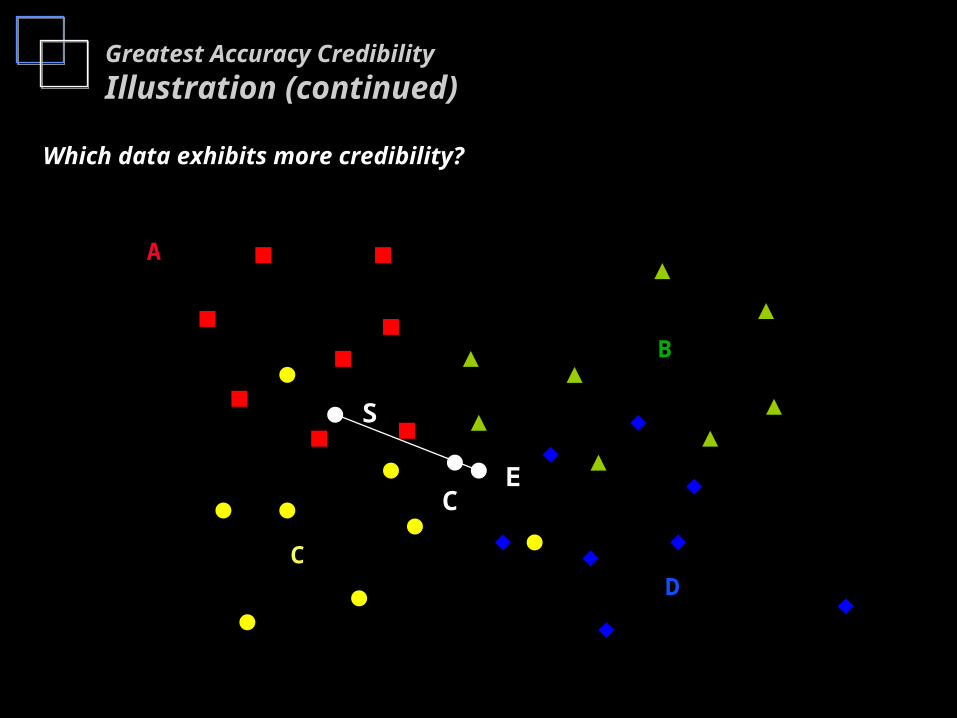
Greatest Accuracy Credibility
Illustration (continued)
Which data exhibits more credibility?
A
D
B
C
E
S
C

Greatest Accuracy Credibility
Illustration (continued)
A DB CE
A DB CE
Class loss costs per exposure...
0
0
Higher credibility: less variance within, more variance between
Lower credibility: more variance within, less variance between

Greatest Accuracy Credibility
Increasing credibility
Per the formula,
Z = n
n + s2
t2
Credibility, Z, can be increased by: Increasing n = get more data decreasing s2 = less variance within classes, e.g., refine data
categories increase t2 = more variance between classes
Greatest Accuracy Credibility
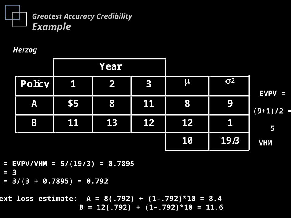
Example
Herzog
Year
Policy 1 2 3 2
A $5 8 11 8 9
B 11 13 12 12 1
10 19/3
EVPV =
(9+1)/2 =
5
VHM
k = EVPV/VHM = 5/(19/3) = 0.7895n = 3Z = 3/(3 + 0.7895) = 0.792
Next loss estimate: A = 8(.792) + (1-.792)*10 = 8.4 B = 12(.792) + (1-.792)*10 = 11.6

Bibliography

Bibliography
Herzog, Thomas. Introduction to Credibility Theory. Longley-Cook, L.H. “An Introduction to Credibility
Theory,” PCAS, 1962 Mayerson, Jones, and Bowers. “On the Credibility
of the Pure Premium,” PCAS, LV Philbrick, Steve. “An Examination of Credibility
Concepts,” PCAS, 1981 Venter, Gary and Charles Hewitt. “Chapter 7:
Credibility,” Foundations of Casualty Actuarial Science.
Introduction to Credibility