Introductionto

Computer Algebra

K. Kalorkoti

School of Informatics

University of Edinburgh

Informatics Forum

10 Crichton Street

Edinburgh EH8 9AB

Scotland

E-mail: kk@inf.ed.ac.uk

January 2019

Preface

These notes are for the fourth year and MSc course in Computer Algebra. They contain morematerial than can fit into the time available. The intention is to allow you to browse through extramaterial with relative ease. If you have time, you are strongly encouraged to follow in detail at leastsome of the extra material. However it will not be assumed that you have done this and success inthe course does not depend on it. The course itself will cover a selection of the topics mentioned,even so some details will be omitted. For example Grobner bases are given quite a full treatment. Inthe course itself more emphasis will be placed on understanding their use, the basic algorithm andthe intuitive explanation of how and why they work. For other topics we will look at the details quiteclosely. Broadly speaking, the examinable parts are those covered in the lectures or assigned forhome reading (the lecture log at the course web page, http://www.inf.ed.ac.uk/teaching/courses/ca,will state the parts of the notes covered). A guide to revision will be handed out at the end of thecourse (and placed on the course web site) stating exactly which topics are examinable.

You will find a large number of exercises in the notes. While they are not part of the formalcoursework assessment (separate exercise sheets will be issued for this) you are strongly encouragedto try some of them. At the very least you should read and understand each exercise. You arewelcome to hand me any of your attempts for feedback; we will in any case discuss some of theexercises in lectures. As a general rule the less familiar you are with a topic the more exercisesyou should attempt from the relevant section. One or more of these exercises will be suggested atthe end of some lectures for you to try. There will be a follow up discussion at the next lectureto provide you with feedback on your attempts. If you find any errors or obscure passages in thenotes please let me know.

Parts of these notes are based on lectures given by Dr. Franz Winkler at the Summer School inComputer Algebra which was held at RISC-LINZ, Johannes Kepler University, Austria, during thefirst two weeks of July, 1990. I am grateful for his permission to use the material.

Note: These notes and all other handouts in the course are for your private study and must not becommunicated to others in any way; breaking this requirement constitutes academic misconduct.

He liked sums,but not the way they were taught.

— BECKETT, Malone Dies

i

Contents

1 Introduction 11.1 General introduction . . . . . . . . . . . . . . . . . . . . . . . . . . . . . . . . . . . . 11.2 Features of Computer Algebra Systems . . . . . . . . . . . . . . . . . . . . . . . . . . 21.3 Syntax of Associated Languages . . . . . . . . . . . . . . . . . . . . . . . . . . . . . . 51.4 Data Sructures . . . . . . . . . . . . . . . . . . . . . . . . . . . . . . . . . . . . . . . 5

2 Brief Introduction to Axiom 52.1 Background . . . . . . . . . . . . . . . . . . . . . . . . . . . . . . . . . . . . . . . . . 52.2 Using the System . . . . . . . . . . . . . . . . . . . . . . . . . . . . . . . . . . . . . . 62.3 Brief Overview of Axiom’s Structure . . . . . . . . . . . . . . . . . . . . . . . . . . . 62.4 Basic Language Features . . . . . . . . . . . . . . . . . . . . . . . . . . . . . . . . . . 72.5 Basic Literature . . . . . . . . . . . . . . . . . . . . . . . . . . . . . . . . . . . . . . . 9

3 Computer Algebra Systems 10

4 Basic Structures and Algorithms 124.1 Algebraic Structures . . . . . . . . . . . . . . . . . . . . . . . . . . . . . . . . . . . . 124.2 Greatest Common Divisors . . . . . . . . . . . . . . . . . . . . . . . . . . . . . . . . 174.3 Canonical and Normal Representations . . . . . . . . . . . . . . . . . . . . . . . . . . 184.4 Integers and Rationals . . . . . . . . . . . . . . . . . . . . . . . . . . . . . . . . . . . 184.5 Integers . . . . . . . . . . . . . . . . . . . . . . . . . . . . . . . . . . . . . . . . . . . 184.6 Fractions . . . . . . . . . . . . . . . . . . . . . . . . . . . . . . . . . . . . . . . . . . 19

4.6.1 Euclid’s Algorithm for the Integers . . . . . . . . . . . . . . . . . . . . . . . . 214.6.2 Worst-Case Runtime of Euclid’s Algorithm . . . . . . . . . . . . . . . . . . . 24

4.7 Polynomials . . . . . . . . . . . . . . . . . . . . . . . . . . . . . . . . . . . . . . . . . 264.7.1 Polynomial Functions . . . . . . . . . . . . . . . . . . . . . . . . . . . . . . . 294.7.2 Digression: Formal Power Series . . . . . . . . . . . . . . . . . . . . . . . . . 304.7.3 Polynomials in Several Indeterminates . . . . . . . . . . . . . . . . . . . . . . 314.7.4 Differentiation . . . . . . . . . . . . . . . . . . . . . . . . . . . . . . . . . . . 324.7.5 Factorization and Greatest Common Divisors . . . . . . . . . . . . . . . . . . 334.7.6 Euclid’s Algorithm for Univariate Polynomials . . . . . . . . . . . . . . . . . 354.7.7 A Remainder Theorem . . . . . . . . . . . . . . . . . . . . . . . . . . . . . . . 374.7.8 Rational Expressions . . . . . . . . . . . . . . . . . . . . . . . . . . . . . . . . 394.7.9 Representation of Polynomials and Rational Expressions . . . . . . . . . . . . 39

5 Keeping the Data Small: Modular Methods 435.1 Modular gcd of Polynomials in Z[x] . . . . . . . . . . . . . . . . . . . . . . . . . . . . 435.2 The Chinese Remainder Problem . . . . . . . . . . . . . . . . . . . . . . . . . . . . . 475.3 Bound on the Coefficients of the gcd . . . . . . . . . . . . . . . . . . . . . . . . . . . 505.4 Choosing Good Primes . . . . . . . . . . . . . . . . . . . . . . . . . . . . . . . . . . . 525.5 Modular gcd Algorithm for Multivariate Polynomials . . . . . . . . . . . . . . . . . . 56

iii

6 Grobner Bases 596.1 Basics of Algebraic Geometry . . . . . . . . . . . . . . . . . . . . . . . . . . . . . . . 596.2 Grobner Bases . . . . . . . . . . . . . . . . . . . . . . . . . . . . . . . . . . . . . . . 656.3 Definition and Characterization of Grobner Bases . . . . . . . . . . . . . . . . . . . . 686.4 Computation of Grobner Bases . . . . . . . . . . . . . . . . . . . . . . . . . . . . . . 736.5 Applications of Grobner Bases . . . . . . . . . . . . . . . . . . . . . . . . . . . . . . 776.6 Improvements of the Basic Grobner Basis Algorithm . . . . . . . . . . . . . . . . . . 806.7 Complexity of Computing Grobner Bases . . . . . . . . . . . . . . . . . . . . . . . . 81

6.7.1 Algebraic Preliminaries . . . . . . . . . . . . . . . . . . . . . . . . . . . . . . 826.7.2 Counting . . . . . . . . . . . . . . . . . . . . . . . . . . . . . . . . . . . . . . 85

6.8 The Case of Two Indeterminates . . . . . . . . . . . . . . . . . . . . . . . . . . . . . 86

1 Real Roots of Polynomials 11.1 Real Root Approximation . . . . . . . . . . . . . . . . . . . . . . . . . . . . . . . . . 1

1.1.1 Square Free Decomposition . . . . . . . . . . . . . . . . . . . . . . . . . . . . 31.2 Real Root Isolation . . . . . . . . . . . . . . . . . . . . . . . . . . . . . . . . . . . . . 4

1.2.1 Counting Real Roots of Univariate Polynomials . . . . . . . . . . . . . . . . . 61.3 Real Root Isolation by Continued Fractions . . . . . . . . . . . . . . . . . . . . . . . 11

1.3.1 The Ruffini–Horner Method . . . . . . . . . . . . . . . . . . . . . . . . . . . . 191.4 Complex Roots . . . . . . . . . . . . . . . . . . . . . . . . . . . . . . . . . . . . . . . 21

8 Bibilography 119

iv

1 Introduction

1.1 General introduction

Consider the expression

f =32x8 − 16x7 + 82x6 − 40x5 + 85x4 − 40x3 + 101x2 − 48x+ 6

8x5 − 2x4 + 4x3 − x2 + 12x− 3(1)

Suppose that we want to differentiate f . In a sense there is no problem at all since we can use theformula

d(p/q)

dx=q dpdx − p

dqdx

q2.

However an attempt to apply this to f by hand leads to quite messy calculations. Even if no errorhappens during these calculations the answer might be needlessly complicated. Indeed a directapplication of the formula to f (with expansion of the products in the numerator) yields

768x12 − 512x11 + 1392x10 − 776x9 + 3152x8 − 1928x7 + 3212x6

−1626x5 + 2768x4 − 1548x3 + 1452x2 − 594x+ 72(8x5 − 2x4 + 4x3 − x2 + 12x− 3)2

.

It might be better to simplify f as much as possible before operating on it. Here the word ‘sim-plify’ denotes the removal of common factors from numerator and denominator. For example theexpression

x4 − 1

x2 + 1

simplifies tox2 − 1

since x4 − 1 = (x2 − 1)(x2 + 1) (we discuss this point in greater detail in §4.7.8). This process israther like that of reducing a fraction a/b to its lowest terms by cancelling out the greatest commondivisor of a and b. In fact it can be seen that the numerator in the right hand side of (1) is equal to

(4x− 1)2(x2 + 2)(2x4 + x2 + 3)

and the denominator is equal to(4x− 1)(2x4 + x2 + 3)

so thatf = (4x− 1)(x2 + 2)

= 4x3 − x2 + 8x− 2

which yieldsdf

dx= 12x2 − 2x+ 8.

The simplification achieved here is quite considerable. The obvious question now is how can we carryout the simplification in general? Indeed do we need to factorize the numerator and denominatoror is there an easier method? Again a comparison with the case for fractions suggests that we donot have to find the factorization (we discuss this in §4.7.6).

1

As another example suppose that we want to integrate

g =x2 − 5

x(x− 1)4.

A little experience shows that such problems can often be solved by decomposing the expressioninto partial fractions. (We say that a fraction c/pq is decomposed into partial fractions if we canwrite it as a/p+ b/q. The summands might themselves be split further into partial fractions. Notethat such a decomposition is not always possible, e.g., 1/x2 cannot be so decomposed.) In our casewe have

g =−5

x+

5

x− 1− 5

(x− 1)2+

6

(x− 1)3− 4

(x− 1)4.

We may now proceed to integrate each of the summands and add the results to obtain the integralof g. Once again the decomposition process is rather tedious and we could easily make a mistake—the same applies to the final process of integration! It is therefore highly desirable to have machineassistance for such tasks. Indeed it would be very useful to be able to deal with more generalexpressions such as

x+ a

x(x− b)(x2 + c)

where a, b, c are arbitrary unspecified constants. More ambitiously we might ask about the possi-bility of integrating expressions drawn from a large natural class. One of the major achievementsof Computer Algebra has been the development of an algorithm that will take an expression fromsuch a class and either return its integral or inform the user that no integral exists within the class.

There are many more applications of Computer Algebra some of which will be discussed as thecourse progresses. The overall aim is the development of algorithms (and systems implementingthem) for Mathematical problem solving. As the examples given above illustrate, we do not restrictattention to numerical problems.

1.2 Features of Computer Algebra Systems

All the well developed Computer Algebra systems are designed to handle a large amount of tra-ditional forms of mathematics such as that used in Engineering applications. Some systems canhandle more abstract Mathematics as well. In this section we outline those capabilities that arefound in the majority of well developed systems. The degree to which problems of a given kind(such as integration) can be solved will vary from one system to the next.

Interactive use

The user can use the system directly from the terminal and see results displayed on the screen. Onold fashioned character terminals the results were shown in a basic 2-dimensional format; this canstill be useful if a system is being used remotely over a slow connection. Systems such as Maplewill produce a much more sophisticated display on modern terminals; Axiom does not yet have asophisticated interface.

2

File handling

Expressions and commands can be read from files. This is clearly essential for the development ofprograms in the system’s language. Output can also be sent to a file. The output can be in variousformats or in a form which is suitable for input back to the system at some later stage.

Polynomial manipulation

Without this ability a system cannot be deemed to be a Computer Algebra system. Polynomialsare expressions such as

4x2 + 2x− 3

orx4 − x3y + 5xy3 − 20y.

Systems can also handle operations on rational expressions (i.e., expressions of the form p/q wherep, q are both polynomials).

Elementary special functions

These include such basics as

• sine, cosine, tangent (and their inverses),

• natural logarithms and exponentials,

• hyperbolic sine, cosine, tangent (and their inverses).

Normally systems can differentiate and integrate expressions in these as well as apply certain sim-plifications such as sin(0) = 0.

Arithmetic

Integer and rational arithmetic can be carried out to any degree of accuracy. (Some systemsimpose an upper limit but this is extremely large. Naturally the available physical storage willalways impose a limit.) In floating point arithmetic the user can specify very high levels of accuracy.Normally systems will use exact arithmetic rather than resort to floating point approximations. Forexample 1/3 will not be converted to an approximation such as 0.33333 unless the user demands

it. Similar remarks apply to such expressions as√

9 + 4√

2. If approximations are used then notonly do we lose precision but might also obtain false results. For example consider the polynomials(taken from [21])

p = x3 − 8

q = (1/3)x2 − (4/3)

Now it can be seen that the polynomial

d = (1/3)x− (2/3)

divides both of these, i.e.,p = (3x2 + 6x+ 12)d

q = (x+ 2)d

3

and moreover no polynomial of degree higher than that of d has this property, i.e., d is a gcd ofp, q. Suppose however that we consider the polynomial

q = 0.333333x2 − 1.33333

which appears to be a good approximation to q. If we now use p and q to find an approximation dto d and use six digit accuracy in arithmetic operations (using a version of Euclid’s algorithm for

polynomial gcd’s) then we obtain d = 0.000001 which is nothing like a good approximation to d.Most systems can also carry out complex number arithmetic.

Differentiation

This can be applied to expressions involving polynomials and special functions which are recognizedby the system. Partial derivatives can also be computed.

Integration

Expressions involving polynomials and special functions can usually be integrated. The expressionscan be quite complicated—the system does much more than just look the result up in a table ofstandard integrals. Integration is one of the most difficult tasks carried out by a Computer Algebrasystem. All systems have some problems with definite integration and occasionally produce wronganswers (indefinite integration is easier). It is important to understand that Computer Algebrasystems treat integration from an algebraic rather than an analytic viewpoint. For most of the timethere is no difference but for certain situations the answer returned is correct only in the algebraicsense (e.g., the integral of a continuous function might be returned as a non continuous one). Thisfact is not appreciated as widely as it ought to be.

Solving equations

Systems of simultaneous linear equations with numeric or symbolic coefficients can be solved exactly.Arbitrary polynomial equations up to degree 4 can also be solved exactly. For higher degree

polynomials no general method is possible (this is a mathematical theorem), however certain typesof equations can still be handled.

First and second order differential equations can usually be solved as well.

Substitution

It is very useful to be able to substitute an expression in place of a given variable. This allows theuser to build up large expressions or alter existing ones in a controlled manner. All systems havethis facility.

Matrices

All systems provide basic operations on matrices. The entries of the matrices do not have to benumerical or even specified. Systems provide methods for initializing large matrices or for buildingspecial types such as symmetric matrices.

4

Mathematical structures

Sophisticated systems such as Axiom enable the user to work (and indeed define for themselves)mathematical structures of many kinds. Thus a user can work with groups, rings, fields, algebrasetc. The underlying system supplies the appropriate operations on elements and many algorithmsfor examining the structure of particular examples thus making it easy to test conjectures of manykinds.

Defining new rules and procedures

Users can define their own functions for tasks which are not covered by the built-in operations. Itis generally possible to define certain properties of the function such as its derivative or integral(where these make sense). Rules for simplifying expressions which involve the function can usuallybe specified as well.

Graphics

Most systems can produce simple plots. With increasing computational power and better displays,most systems have introduced highly developed capabilities for plotting mathematical functionsin 2 or 3 dimensions (in black and white or colour and specified illumination for 3D).

1.3 Syntax of Associated Languages

These are mostly Algol-like, with more recent influences. A little experience with a language suchas C provides sufficient background for a quick mastery of a Computer Algebra system’s language.All the general purpose systems allow users to define their own procedures thus extending thesystem.

Most systems provide a notion of type but this is at times an add on to the original design andthe default mode is to work without types. By contrast types are at the core of Axiom.

1.4 Data Sructures

All systems supply a large number of built in data structures, ranging rom purely mathematicalones such as polynomials, infinite series or matrices to general ones such as lists, arrays, hash tablesor trees. There are over 40 kinds of aggregate data structures in Axiom.

2 Brief Introduction to Axiom

2.1 Background

The brief history of Axiom at http://www.axiom-developer.org can be summarised as follows. Ax-iom is a system for symbolic mathematical computation which started in 1971 as an IBM projectunder the name Scratchpad. In the 1990’s it was sold to the Numerical Algorithms Group (NAG)and marketed under the name Axiom. However it did not become a financial success and was with-drawn from the market in October 2001. Shortly after this it was released as free software with the

5

source being available at https://github.com/daly/axiom. For more details see http://www.axiom-developer.org and the introduction to the free book at http://www.axiom-developer.org/axiom-website/bookvol1.pdf (which you should download). In fact there are now at least two open sourceversions of Axiom, this course will follow the one given at the preceding links.

2.2 Using the System

Simply log on to a linux machine and type axiom, alternatively download and install it on your ownmachine. We have tested it on linux and Mac, the Axiom site also has instructions for Windowsbut we have not tested these.

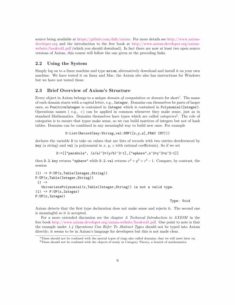
2.3 Brief Overview of Axiom’s Structure

Every object in Axiom belongs to a unique domain of computation or domain for short1. The nameof each domain starts with a capital letter, e.g., Integer. Domains can themselves be parts of largerones, so PositiveInteger is contained in Integer which is contained in Polynomial(Integer).Operations names ( e.g., +) can be applied in common whenever they make sense, just as instandard Mathematics. Domains themselves have types which are called categories2. The role ofcategories is to ensure that types make sense, so we can build matrices of integers but not of hashtables. Domains can be combined in any meaningful way to build new ones. For example

D:List(Record(key:String,val:DMP([x,y,z],FRAC INT)))

declares the variable D to take on values that are lists of records with two entries dereferenced bykey (a string) and val (a polynomial in x, y, z with rational coefficients). So if we set

D:=[["parabola", (x/a)^2+(y/b)^2-1],["sphere",x^2+y^2+z^2-1]]

then D.2.key returns "sphere" while D.2.val returns x2 + y2 + z2− 1. Compare, by contrast, thesession

(1) -> P:UP(x,Table(Integer,String))

P:UP(x,Table(Integer,String))

1) ->

UnivariatePolynomial(x,Table(Integer,String)) is not a valid type.

(1) -> P:UP(x,Integer)

P:UP(x,Integer)

Type: Void

Axiom detects that the first type declaration does not make sense and rejects it. The second oneis meaningful so it is accepted.

For a more extended discussion see the chapter A Technical Introduction to AXIOM in thefree book http://www.axiom-developer.org/axiom-website/bookvol1.pdf. One point to note is thatthe example under 1.4 Operations Can Refer To Abstract Types should not be typed into Axiomdirectly; it seems to be in Axiom’s language for developers but this is not made clear.

1These should not be confused with the special types of rings also called domains, that we will meet later on.2These should not be confused with the objects of study in Category Theory, a branch of mathematics.

6

2.4 Basic Language Features

Like other computer algebra systems Axiom has its own programming language. Most of its con-structs will be familiar from other imperative languages, e.g., loops, conditional statements, recur-sion. The format of loops is quite flexible allowing for convenient expression of ideas. Here aresome examples:

(1) -> for i in 1..5 repeat print(i^i)

1->

4

27

256

3125

Type: Void

(2) -> L:=[1,2,3,4,5]

L:=[1,2,3,4,5]

(2) ->

(2) [1,2,3,4,5]

Type: List(PositiveInteger)

(3) -> for i in L repeat print(i^i)

for i in L repeat print(i^i)

1->

4

27

256

3125

Type: Void

(4) -> L:=[i for i in 1..10]

L:=[i for i in 1..10]

(4) ->

(4) [1,2,3,4,5,6,7,8,9,10]

Type: List(PositiveInteger)

(5) -> for i in L repeat print(i^i)

for i in L repeat print(i^i)

1->

4

27

256

3125

46656

823543

16777216

387420489

10000000000

Type: Void

In the second and third examples L is a list which we create in two different ways (lines (2) and (4)).There are many data structures built in with supporting operations.

7

As can be seen from the session above Axiom is a typed language. Indeed it was an early adopterof the notion of inheritance so that operations common to various types can become more specialisedas the data type does so. However the user is not forced to declare the type of everything, the systemwill try to deduce the information, thus freeing users to work fluently. At times the system is unableto deduce the type (either because of insufficient information or it is too complicated); if so the useris informed and has the opportunity to supply the information. Here is an example of a functiondefinition from Axiom:

(1) -> f(0)==0

f(0)==0

Type: Void

(2) -> f(1)==1

f(1)==1

Type: Void

(3) -> f(n)==f(n-1)+f(n-2)

f(n)==f(n-1)+f(n-2)

Type: Void

(4) -> f(10)

f(10)

Compiling function f with type Integer -> NonNegativeInteger

Compiling function f as a recurrence relation.

^

... (a lot of messages deleted [KK])

(4) 55

Type: PositiveInteger

(5) -> f(1000)

f(1000)

(5) ->

(5)

4346655768693745643568852767504062580256466051737178040248172908953655541794_

905189040387984007925516929592259308032263477520968962323987332247116164299_

6440906533187938298969649928516003704476137795166849228875

Type: PositiveInteger

(6) ->

Clearly f is the Fibonacci function. We define it piecewise just as would be done in a maths book.The sign == is delayed assignment, in effect it tells Axiom not to evaluate anything at this time butto use the right hand side when required (it does carry out various checks, e.g., that types makesense). On the first call Axiom gathers together the piecewise definition of f and tries to compile it,in this case successfully. During compilation it carries out some optimisations so that in this casecomputing f is done efficiently (a naive version would involve exponentially many recursive calls).If the function cannot be compiled (e.g., the system cannot determine the types of the arguments)it is interpreted instead.

Finally, Axiom makes polymorphic functions available so that the same code will be compiledas appropriate for different data types. Here is a simple example:

(1) -> first(L)==L.1

first(L)==L.1

8

Type: Void

(2) -> first([1,2,3])

first([1,2,3])

Compiling function first with type List(PositiveInteger) ->

PositiveInteger

... (a lot of messages deleted [KK])

(2) 1

Type: PositiveInteger

(3) -> first([1,x,x^2])

first([1,x,x^2])

Compiling function first with type List(Polynomial(Integer)) ->

Polynomial(Integer)

... (a lot of messages deleted [KK])

(3) 1

Type: Polynomial(Integer)

On subsequent calls of, e.g., first([1,2,3]) and first([1,x,x^2]) no further compilation isnecessary; the appropriate compiled code is used.

2.5 Basic Literature

The following is a short list of references together with some comments. A much longer list is givenat the end of the notes.

1. B. Buchberger, G. E. Collins and R. Loos (editors), Symbolic and Algebraic Computation.Computing Supplementum 4, Springer (1983).

This book is a collection of articles written by well known people in the field. Many topicsare covered, some of them in great detail. It is essential reading for somebody who wants topursue the field further although certain parts of it are now out of date.

2. J. H. Davenport, Y. Siret and E. Tournier, Computer Algebra; systems and algorithms foralgebraic computation, Academic Press, (1988).

This is one of the first text books on the area (and the only one at a relatively low price). Thecoverage is quite comprehensive and includes many advanced topics. It does not deal withimplementation issues in any depth but some discussion is included. There is an appendixgiving some of the algebraic background which is essential for the subject. There is also anannex which can act as a basic reference manual for the system REDUCE.

Unfortunately there is a tendency to skip details—this is unavoidable in a book of reasonablesize with such a breadth of coverage. More seriously there are quite a few misprints althoughmost are fairly obvious.

3. K. O. Geddes, S. R. Czapor and G. Labahn, Algorithms for Computer Algebra, Kluwer Aca-demic Publishers (1992).

This book is comprehensive and is a good reference for the area. The authors are long-standing members of the Maple group, however the book itself is not Maple centred rather it

9

is concerned with the core algorithms of the area. Unfortunately it is very expensive, howeverthere is a copy in the library.

4. R. Zippel, Effective Polynomial Computation, Kluwer Academic Publishers (1993).

This book focuses on the core polynomial operations in Computer Algebra and studies themin depth. It is a good place to go to for extra detail (both theoretical and practical). Unfor-tunately it has a fairly large number of misprints most of which are minor (a list is availablefrom K. Kalorkoti).

5. D. E. Knuth, Seminumerical Algorithms, (Second Edition), Addison-Wesley (1981).

Chapter 4 gives a comprehensive treatment of topics in arithmetic and some aspects of poly-nomial arithmetic. Although the course will not go into such staggering detail every seriousstudent of computing should consult this book. Several copies are available from the library.

6. T. H. Cormen, C. E. Leiserson, R. L. Rivest, and C. Stein, Introduction to Algorithms.McGraw-Hill, 2002 (now in its third edition, published September 2009).

This book is not specifically related to Computer Algebra, however it is an excellent sourcefor many algorithms and general background. There are also several chapters on basic Math-ematics.

7. D. R. Stoutemyer, Crimes and misdemeanors in the computer algebra trade, Notices of theAMS, Sept. 1991, 701-705.

This paper describes some of the ways in which computer algebra systems can produce wrongresults. Ideally it (or something like it) should be read by every user of such systems. Acrude but effective summing up of some of the paper is that having a computer does not giveyou the right to throw your brain away—quite the opposite is true. The paper concentrateson analysis rather than algebra, surprisingly the author does not discuss newer systems suchas Scratchpad II (now called AXIOM) which try to be more sensible about the domain ofcomputation. (In this course we will be concerned almost exclusively with the algebraicviewpoint.)

8. F. Winkler, Polynomial Algorithms in Computer Algebra, Springer (1996).

This book is devoted to algebraic aspects of the subject, ranging from basic topics to algebraiccurves.

9. J. von zur Gathen and J. Gerhard, Modern Computer Algebra, Cambridge University Press(1999).

This book gives comprehensive coverage to the basics of the subject, aiming at a complete pre-sentation of mathematical underpinnings, analysis of algorithms and development of asymp-totically fast methods.

3 Computer Algebra Systems

Below is a list of some systems in addition Axiom.

10

• Macsyma: started at MIT under the direction of J. Moses. A very large system. A majordrawback is that it has had too many implementors with no common style and there is nosource code documentation. It is therefore difficult to build on the system using the sourcecode. Macsyma was marketed by Symbolics Inc. for many years. It is now available asMaxima under the GPL license.

• REDUCE: started at the University of Utah under the direction of A. Hearn later of the RandCorporation, Santa Monica. It has many special functions for Physics and is now availableunder a BSD license.

• ALDES/SAC-II (then SACLIB): under the direction of G. E. Collins, University of Wisconsin,Maddison (later at RISC, University of Linz). Originally implemented in Fortran and now inC, the user languages is called ALDES. The system is not very user friendly, it is intendedfor research in Computer Algebra, many basic algorithms were implemented in it for the firsttime. It is still being developed.

• muMath/Derive: developed specifically for micros with limited memory by Soft Warehouselater owned by Texas Instruments. Derive was menu driven and replaced muMath. It wasdiscontinued in June 2007.

• Maple: started at the University of Waterloo, Canada, in the early 1980’s. It is a powerfuland compact system which is ideal for multi-user environments and is still under very activedevelopment.

• Mathematica: this is a product of Wolfram Research Inc., based in Ilinois, and is the successorto SMP. It was announced with a great deal of publicity in Summer 1988. One very strikingfeature at the time was its ability to produce very high quality graphics. Its programminglanguage attempts to mix just about all possible paradigms, this does not seem like a goodidea to me. It is still been developed.

• Sage: this is not strictly speaking a computer algebra system but a wrapper for various freesystems. The front page of the web site (http://www.sagemath.org) states ‘SageMath is a freeopen-source mathematics software system licensed under the GPL. It builds on top of manyexisting open-source packages: NumPy, SciPy, matplotlib, Sympy, Maxima, GAP, FLINT, Rand many more. Access their combined power through a common, Python-based language ordirectly via interfaces or wrappers.’

There are various other more specialised systems, e.g., GAP and Magma for group theory (GAP isavailable through Sage).

11

4 Basic Structures and Algorithms

4.1 Algebraic Structures

We describe some abstract algebraic structures which will be useful in defining various concepts.At first they appear rather dry and daunting but they have their origins in concrete applications(for example groups and fields were shown by Galois to have a deep connection with the problemof solving polynomial equations in radicals when the concepts were still just being formed—seeStewart [57]). We shall use the following standard notation:

1. Z, the integers,

2. Q, the rationals,

3. R, the reals,

4. C, the complex numbers,

5. Zn the integers modulo n where n > 1 is a natural number.

A binary operation on a set R is simply a function which takes two elements of R and returns anelement of R, i.e., a function R × R → R. We normally use infix operators such as ◦, ×, ∗, + forbinary operations. For example addition, subtraction and multiplication are all binary operationson R (division is not a binary operation on R because it is undefined whenever the second argumentis 0). A binary operation ◦ on R is commutative if

x ◦ y = y ◦ x, for all x, y ∈ R.

We say that ◦ is associative if

(x ◦ y) ◦ z = x ◦ (y ◦ z), for all x, y, z ∈ R.

Thus the addition of numbers is both commutative and associative, while subtraction is neither.On the other hand matrix multiplication is associative but not commutative (except in the case of1× 1 matrices with entries whose multiplication is commutative).

Associative operations make notation very easy because it can be shown that any valid way ofbracketing the expression

x1 ◦ x2 ◦ · · · ◦ xnleads to the same result. (The proof of this makes a useful exercise in induction.)

A ring is a set R equipped with two binary operations +, ∗ called addition and multiplicationwith the following properties:

1. + is associative,

2. + is commutative,

3. there is a fixed element 0 of R such that x+ 0 = x for all x ∈ R,

4. for each element x of R there is an element y ∈ R such that x+ y = 0, (i.e., x has an additiveinverse),

12

5. ∗ is associative,

6. for all x, y, z ∈ R we havex ∗ (y + z) = x ∗ y + x ∗ z,(x+ y) ∗ z = x ∗ z + y ∗ z,

i.e., ∗ is both left and right distributive over +.

It is important to bear in mind that R need not be a set of numbers and even if it is the two binaryoperations might be different from the usual addition and multiplication of numbers (in which casewe use symbols which are different from + and ∗ in order to avoid confusion). The element 0 iseasily seen to be unique and is called the zero of the ring. We prove this claim by the usual method:suppose there are two elements 0, 0′ that satisfy the axioms for zero. Then

0′ = 0′ + 0, by axiom 3

= 0 + 0′, by axiom 2

= 0, since 0′ satisfies axiom 3 by assumption.

Thus 0′ = 0 as claimed. Moreover every x has exactly one additive inverse which is denoted by −x.We normally write x−y instead of the more cumbersome x+(−y). The axioms immediately implycertain standard identities such as x ∗ 0 = 0 for all x. To see this note that x ∗ 0 = x ∗ (0 + 0) =x ∗ 0 + x ∗ 0. Now adding −(x ∗ 0) to both sides we obtain 0 = x ∗ 0 as required. Similarly 0 ∗ x = 0for all x (remember that ∗ is not assumed to be commutative so this second identity does not followimmediately from the first).

It is worth noting that multiplication in rings is frequently denoted by juxtaposition. Thus wewrite xy rather than x ∗ y.

The archetypal ring is Z with the usual addition and multiplication. Other examples include:

1. Q, R, C with the usual addition and multiplication.

2. 2Z the set of all even integers with the usual addition and multiplication.

3. Zn the integers modulo n where n > 1 is a natural number. Here addition and multiplicationare carried out as normal but we then take as result the remainder after division by n.Alternatively we view the elements of Zn to be the integers and use ordinary addition andmultiplication but interpret equality to mean that the two numbers involved have the sameremainder after division by n. More accurately the elements are equivalence classes where twonumbers are said to be equivalent if they have the same remainder when divided by n (thisis the same as saying that their difference is divisible by n). The classes are {kn+ r | k ∈ Z},for 0 ≤ r ≤ n − 1. For simplicity we denote such a class by r. We could use any otherelement of each class to represent it. A simple exercise shows that doing operations based onrepresentatives is unambiguous, that is we always get the same underlying equivalence class.

We will see later on that this is a particular case of a more general construction that gives usa new ring from the ingredients of an existing one. Just to give a hint of this, note that theset nZ = {nm | m ∈ Z} is itself a subring of Z (actually all we need is that it is a two sidedideal but this will have to wait). Note that n can be arbitrary for this construction. Now ifwe define the relation ∼ on Z by

a ∼ b⇔ a− b ∈ nZ

13

we obtain an equivalence relation and use Z /nZ to denote the equivalence classes. Let usdenote the equivalence class of an integer r by [r]; note that by definition [r] = {mn+ r | m ∈Z}.We can turn Z /nZ into a ring by defining + and ∗ on equivalence classes by

[r] + [s] = [r + s],

[r] ∗ [s] = [r ∗ s].

There is a subtlety here, we must show that the operations are well defined, i.e., if [r1] = [r2]and [s1] = [s2] then [r1] + [s1] = [r2] + [s2] and [r1] ∗ [s1] = [r2] ∗ [s2]. This is quite easy to dobut we will leave it for the general case (this is where we need the substructure nZ to be asubring, in fact just a two sided ideal).

The use of square brackets to denote equivalence classes is helpful at first but soon becomestedious. In practice we drop the brackets and understand from the context that an equivalenceclass is being denoted. This is an important convention to get used to; the meaning of a pieceof notation depends on the structure in which we are working. Thus if we are working overthe integers then 3 denotes the familiar integer (“three”) but if we are working in the integersmodulo 6 then it denotes the set of integers {6m+3 | m ∈ Z}. Finally, we have used Zn as anabbreviation for Z /nZ. This is quite standard but in more advanced algebra the notation isnot so good because it conflicts with the notation of another very useful concept (localization,since you ask).

4. Square matrices of a fixed size with integer entries. Here we use the normal operations ofmatrix addition and matrix multiplication.

Again this is a particular case of a general construction, we can form a ring by consideringsquare matrices with entries from any given ring.

5. Let S be any set and P = P(S) the power set of S (i.e., the set of all subsets of S). Thisforms a ring where

• Addition is symmetric difference, i.e., A+B is A∪B−A∩B (this consists of al elementsthat are in one of the sets but not both).

• Multiplication is intersection, i.e., A ∗B is A ∩B.

The empty set plays the role of 0. This is an example of a Boolean ring, i.e. x ∗ x = x forall x.

Note that in all our examples, except for matrices, multiplication is also commutative. A ring whosemultiplication is commutative is called commutative. Notice further that in all our examples, exceptfor the ring 2Z (generally nZ for n > 1), we have a special element 1 with the property that

1x = x1 = x, for all x ∈ R.

An element with this property is called a (multiplicative) identity of the ring. In fact it is easilyseen that if such an identity exists then it is unique. (There is a clear analogy with 0 here which isan additive identity for the ring—however the existence of 0 in a ring is required by the axioms).

While the definition of rings is clearly motivated by the integers, certain ‘strange’ things canhappen. For example in Z6 we have 2× 3 = 0 even though 2 6= 0 and 3 6= 0 in Z6 (i.e., 6 does notdivide 2 or 3). Matrix rings also exhibit such behaviour.

14

Pursuing the numerical analogy one level up we see that in the ring Q every non-zero elementhas a multiplicative inverse, i.e., for each x 6= 0 there is a y ∈ Q such that xy = yx = 1. Ofcourse in general the notion of a multiplicative inverse only makes sense if the ring has an identity.However even if the ring does have an identity there is no guarantee that particular elements willhave inverses. For example in the ring of 2× 2 matrices with integer entries we observe that(

1 00 0

)does not have an inverse. Note that (

1 00 2

)also does not have an inverse in our ring although it does have an inverse in the ring of 2 × 2matrices with entries from Q. It is easy to show that if an element x of a ring R has an inversethen it is unique (and is normally denoted by x−1).

Exercise 4.1 Write the multiplication tables of Z2, Z3, Z4, Z5, Z6 and decide which elements havean inverse for each of these rings. Can you spot a pattern?

Observations such as the above lead to the notion of fields. A field is a ring with the extra properties

1. there is a multiplicative identity which is different from 0,

2. multiplication is commutative,

3. every non-zero element has an inverse,

This brings the behaviour of our abstract objects much closer to that of numbers. However ‘strange’things can still happen. For example it is easy to see that Z2 is a field but in here we have 1+1 = 0.Certain other types of behaviour are definitely excluded, for example if xy = 0 then x = 0 or y = 0;for if x 6= 0 then it has a multiplcative inverse and so we have

y = (x−1x)y = x−1(xy) = x−10 = 0.

Examples of fields include:

1. Q, R, C all with the usual operations.

2. Zp when p is a prime.

Exercise 4.2 Show that Zn is not a field whenever n is not a prime number. Treat n = 1 as aspecial case and then consider composite n for n > 1. (Hint: in a field there cannot be non-zeroelements x, y such that xy = 0, as shown above.)

Exercise 4.3 We have seen that in certain fields it is possible to obtain 0 by adding 1 to itselfsufficiently many times. The characteristic of a field is defined to be 0 if we can never obtain 0 inthe way described and otherwise it is the least number of times we have to add 1 to itself in orderto obtain 0. Show that every non-zero characteristic is a prime number.

15

Fields bring us closer to number systems such as Q and R rather than Z. One reason for this isbecause in a field every non-zero element must have an inverse. We can define other types of ringswhich don’t go this far. An integral domain (or ID) is a commutative ring with identity (differentfrom zero) with the property that if xy = 0 then x = 0 or y = 0. (Of course every field is an ID butnot conversely.) A still more specialized class of rings consists of the unique factorization domains(or UFD’s). We shall not give a formal definition of these but explain the idea behind them. It iswell known that every non-zero integer n can be factorized as a product of prime numbers:

n = p1p2 · · · ps.

(Here we allow the possibility of negative ‘primes’ such as −3.) Moreover if we have anotherfactorization of n into primes

n = q1q2 · · · qt,

then

1. s = t, and

2. there is a permutation π of 1, 2, 3, . . . , s such that pi = εiqπ(i) for 1 ≤ i ≤ n where εi = ±1.

Note that ±1 are the only invertible elements of Z. The notion of a prime or rather irreducibleelement can be defined for ID’s: a non-zero element a of an ID is irreducible if it does not have aninverse and whenever a = bc then either b or c has a multiplicative inverse.

Note that if u is an invertible element of a ring and a is any element of the ring then we havea = u(u−1a) which is a trivial ‘factorization.’ Such a ‘factorization’ tells us nothing about a. Forexample writing 6 = −1×−6 contains no information about 6. Writing 6 = 2× 3 gives us genuineinformation about 6 since neither factor is invertible in Z and so the factorization is not automatic.This discussion also shows that factorization is not an interesting concept for fields; every non-zeroelement is invertible. You have known this for a long time though perhaps not in this abstractsetting; you would never consider if a rational or a real number has a factorization.

A UFD is an ID in which every non-zero element has a factorization in finitely many irreducibleelements and this factorization is unique in a sense similar to that for integer factorization. Ob-viously Z is a UFD. Also every field is a UFD for the trivial reason that in a field there are noprimes (every non-zero element has an inverse) so that each non-zero element factorizes uniquelyas its (invertible) self times the empty product of irreducible elements! In a UFD we have a veryimportant property. Let us say that b divides a, written as b | a, if a = bc for some c. It can beshown that if p is irreducible and p | ab then either p | a or p | b (in fact this property is usually takenas the definition of a prime element in a ring—the observation then says that in a UFD irreducibleelements are primes, see Exercise 4.4 for an example of a ring in which irreducible elements neednot be primes).

Exercise 4.4 This exercise shows that unique factorization really is a special property which canfail even in rings which seem quite innocuous. Let Z[

√−5] be the set of all elements

{ a+ b√−5 | a, b ∈ Z }.

It is clear that Z[√−5] becomes a ring under the usual arithmetic operations—indeed it is an ID

since it just consists of numbers with the usual operations.

16

1. Show that 3, 2 +√−5 and 2−

√−5 are all irreducible elements of Z[

√−5].

So for this part you need to show that, e.g., if 3 = (a1 + b1√−5)(a2 + b2

√−5) then one

of the factors is invertible. You can make life easier by noting two things: firstly we have(a+ b

√−5)(a− b

√−5) = a2 + 5b2. Secondly a1 + b1

√−5 = a2 + b2

√−5 if and only if a1 = a2

and b1 = b2, this follows from the fact that√−5 is not a real number (all we need is that it

is not rational).

2. Observe that 3 × 3 = (2 +√−5)(2 −

√−5) so that 3 | (2 +

√−5)(2 −

√−5). Show that 3

does not divide either of 2 +√−5 or 2 −

√−5 (remember that everything takes place inside

Z[√−5]).

3. Deduce that the ID Z[√−5] is not a UFD.

4.2 Greatest Common Divisors

Let a, b be elements of an integral domain D. We call d ∈ D a common divisor of a, b if d | aand d | b. Such a common divisor is called a greatest common divisor (gcd) if whenever c is also acommon divisor of a, b then c | d. (Intuitively speaking a gcd contains all the common factors ofthe two elements concerned, so long as at least one of them is non-zero.)

Note that the preceding definition makes sense even if a = b = 0. In this case everything(including 0) divides a and b so is a candidate to be a gcd. However only 0 can actually be a gcdfor if c 6= 0 then 0 6 | c: that is there is no c′ ∈ D such that c = c′ · 0. Hence the second condition fora gcd is satisfied only by 0 and this is the unique gcd in this case. Moreover if a 6= 0 or b 6= 0 then 0cannot be a gcd for then either 0 6 | a or 0 6 | b. Hence the only time 0 is a gcd is when both inputsare themselves 0. It is worth noting how this definition is more general than the standard one forthe gcd of two integers: there we normally say that the gcd is the largest integer that divides bothinputs, but if they are both 0 there is no such largest integer. In the case when at least one inputis not 0 the two definitions agree (provided we insist the gcd is positive). Clearly the problem offinding the gcd is trivial when both inputs are 0 so in developing algorithms we will assume thatat least one input is not zero.

Suppose that d is a gcd of a, b and u is any invertible element of D. Then it is easy to seethat ud is also a gcd of a, b (we have a = rd, b = sd for some r, s ∈ D and so a = (ru−1)(ud),b = (su−1)(ud)). In fact this level of ambiguity is all there is. First of all if the gcd is 0 then this isthe only candidate so the claim is clearly true. If 0 is not the gcd, assume that d1 and d2 are twogcd’s of a, b then there are u1, u2 ∈ D such that d1 = u2d2 and d2 = u1d1, since d1 | d2 and d2 | d1.Now we have d1 = u2d2 = u2u1d1 and since D is an integral domain and d1 6= 0 we may deducethat u1u2 = 1, i.e., u1 and u2 are invertible elements of D.

In general there is no guarantee that gcd’s exist. However if D is a UFD then we can be certainof their existence. In such cases we use gcd(a, b) to denote a gcd of a, b bearing in mind that ingeneral this does not denote a unique element (but all the possibilities are related to each other asdiscussed above). This is not normally a problem because when the notation is used we are willingto accept any of the possible gcd’s. In some cases we can pick a particular candidate, by insistingon some extra property, so that gcd(a, b) denotes a unique element: for example in the case ofthe integers there are only two candidates one of which is positive and the other negative (recallthat the only invertible elements of Z are 1 and −1). Here we make gcd(a, b) unique by choosingthe positive possibility. One convention that we shall always use is that whenever the gcd of two

17

elements is an invertible element of D then we will normalize it to be 1, the multiplicative identity(of course this is fine since if u is a gcd of a, b and u is invertible then uu−1 = 1 is also a gcd of a, b).

In general we say that a, b are coprime (or relatively prime) if gcd(a, b) = 1. It is easy to showthat if a, b are coprime and b | ac then b | c. Under the same assumption, if a | c and b | c then ab | c.

We shall discuss the notion of gcd’s in more detail for those cases of particular interest to us. Ineach of these cases it is possible to give an alternative equivalent definition but it is useful to knowthat a unified treatment is possible.

4.3 Canonical and Normal Representations

A representation in which there is a one to one correspondence between objects and their repre-sentations is often termed canonical. When using a canonical representation, equality of objectsis the same as equality of representations. Clearly this is a desirable feature. Unfortunately it isnot always possible to find canonical representations in an effective way. This might be becausethe problem is computationally unsolvable (remember the halting problem) or computationallyintractable.

The basic objects of Computer Algebra come from Mathematical structures in which we have anotion of a zero object and of subtraction. Under these conditions we can look for a weaker form ofrepresentation—one in which the object 0 has exactly one representation while other objects mighthave several. Such representations are called normal . If we have normal forms then we can testequality of two objects a, b by computing the representation of a− b and testing it for equality (asa representation) with the unique form for 0.

4.4 Integers and Rationals

The great nineteenth century mathematician Kronecker stated ‘God made the integers: all the restis the work of man’. Some people would question Kronecker’s assertion that God exists while otherswould claim that God’s mistake was to add man to the integers. In any case computer algebrasystems must be able to deal with true integers rather than the minute subrange offered by manylanguages.

4.5 Integers

In representing non-negative integers we fix a base and then hold the digits either in a linked listor an array (for the latter option we need a language such as C that enables us to grow arraysat runtime). Leading zeros are suppressed (i.e., 011 loses the 0) in order to have a canonicalrepresentation (we need to have a special case for 0 itself). The base chosen is usually as large aspossible subject to being able to fit the digits into a word of memory and leave one bit to indicatea carry in basic operations (otherwise the carry has to be retrieved in ways that are too machinedependent). Usually the base is a power of 2 or of 10. Powers of 2 make some operations moreefficient while powers of 10 make the input and output of integers more efficient.

Knuth [39] gives a great deal of detail on algorithms for the basic arithmetic operations on largeintegers. Here we look only at multiplication. The classical method uses around n2 multiplicationsof digits and n additions so its cost is proportional to n2. We can do better than this by usingKaratsuba’s algorithm [36]. For simplicity we consider two integers x, y represented in base B

18

both of length n and putx = aBn/2 + b,

y = cBn/2 + d,

(with appropriate adjustment if n is odd). Then

xy = acBn + (bc+ ad)Bn/2 + bd.

Instead of doing one multiplication of integers of length n (costing ∼ n2 time we do four multipli-cations of integers of length n/2 (which costs ∼ 4(n/2)2 = n2). But we don’t have to compute thefour products since

bc+ ad = (a+ b)(c+ d)− ac− bd

and so we only need three products of integers of length n/2 (or possibly n/2 + 1) and then someshifts and additions (costing ∼ n time). Using the algorithm recursively we find that the time T (n)taken to multiply two integers of length n is given by the recurrence

T (n) =

{Θ(1), if n = 1,3T (n/2) + Θ(n), if n > 1.

The solution to this isT (n) = Θ(nlog2 3).

Note that log2 3 ≈ 1.67. We therefore have

Theorem 4.1 Multiplication of integers of length n can be done in time proportional to nlog2 3.

Knuth [39] shows that the method can be refined to prove

Theorem 4.2 For each ε > 0 there is an algorithm for multiplying integers of length n in timeproportional to n1+ε.

Many Computer Algebra systems use the basic Karatsuba algorithm (the refined version is notreally practical). This pays off for numbers of sufficiently many digits (this is implementationdependent) and so the classical method is used for smaller numbers. (Bear in mind that whatconstitutes a ‘digit’ depends on the base.) An asymptotically faster method is due to Schonhageand Strassen [56] which takes time proportional to n log n log log n. Unfortunately the constantinvolved is large and so Computer Algebra systems do not use this method.

4.6 Fractions

These can be represented in any structure that can hold two integer structures (or pointers tothem). Thus a fraction a/b could be denoted generically as 〈a, b〉. We normally insist on thefollowing conditions:

1. The second integer is positive so the sign of the fraction is determined by that of a.

2. The gcd of the two integers is 1.

19

The gcd of a, b is undefined if both a, b are 0 and is the largest positive integer d that dividesboth a and b otherwise (d always exists—why?). This method gives a canonical form and has theadvantage of keeping the size of the two integers as small as possible. We discuss the computationof gcd’s in §4.6.1.

Carrying out arithmetic on rational numbers is straightforward but even here a little thoughtcan improve efficiency. Let a/b and c/d be fractions in their lowest terms with b, c > 0. Then

a

b× c

d=ac

bd=ac/ gcd(ac, bd)

bd/ gcd(ac, bd)

and the last expression is in canonical form. However the fact that gcd(a, b) = gcd(c, d) = 1 meansthat

gcd(ac, bd) = gcd(a, d) gcd(b, c).

If we putd1 = gcd(a, d)

d2 = gcd(b, c)

then(a/d1)(c/d2)

(b/d2)(d/d1)

gives us the canonical form for a/b. This method requires two gcd computations. However this isnot slower than the previous method. We will see in §4.6.1 that the number of ‘basic steps’ of theusual algorithm for computing gcd’s is essentially proportional to the logarithm of the largest ofits inputs. Thus the number of basic steps needed to compute d1 and d2 is roughly the same as isrequired to compute gcd(ac, bd). Each basic step operates on numbers whose size decreases witheach step. It follows that the second method is potentially faster because it works with smallernumbers than the first.

Division is essentially identical to multiplication.For addition and subtraction let

a

b± c

d=p

q

where p/q is in canonical form. Generally it is best to compute p′, q′ by

p′ = ad

gcd(b, d)+ c

b

gcd(b, d)

q′ =bd

gcd(b, d)

and thenp = p′/ gcd(p′, q′), q = q′/ gcd(p′, q′).

Exercise 4.5 Computing q′ by u := bd, v := gcd(b, d), q′ = u/v is a bad idea. Suggest a bettermethod (we assume that gcd(b, d) is already known).

20

4.6.1 Euclid’s Algorithm for the Integers

Recall that the gcd of a, b is 0 if both a, b are 0 and is the largest positive integer d that dividesboth a and b otherwise. We will now assume that at least one of a, b is non-zero. We note thefollowing obvious properties of the gcd function.

1. gcd(a, b) = gcd(b, a).

2. gcd(a, b) = gcd(|a|, |b|).

3. gcd(0, b) = |b|.

4. gcd(a, b) = gcd(a− b, b).

Exercise 4.6 Prove each of the preceding properties of gcd’s.

From now on we shall assume that a, b are non-negative. The various equations suggest the following(impractical) method of finding gcd(a, b).

1. If a = 0 then return b.

2. If a < b then return gcd(b, a).

3. Otherwise return gcd(a− b, b).

Note that this process always halts with a = 0 (why?). There is one obvious improvement that issuggested by the fact that

gcd(a, b) = gcd(a− b, b) = gcd(a− 2b, b) = . . . = gcd(a− qb, b)

for any integer q. In particular if b > 0 and we put

a = qb+ r

where 0 ≤ r < b and q is an integer then

gcd(a, b) = gcd(b, r).

We usually call q the quotient of a, b and r the remainder or residue. This frequently reduces thenumber of subtractions we carry out at the expense of introducing an integer division. Thus wemay find gcd(9, 24) = 3 by

24 = 2× 9 + 6

9 = 1× 6 + 3

6 = 2× 3 + 0

In general we put r0 = a, r1 = b and write

r0 = q1r1 + r2

r1 = q2r2 + r3

r2 = q3r3 + r4

...

rs−2 = qs−1rs−1 + rs

rs−1 = qsrs + rs+1

21

where rs+1 = 0 and 0 ≤ ri < ri−1 for 1 ≤ i ≤ s+ 1. Note that we must eventually have ri = 0 forsome i since r0 > r1 > . . . > rs > rs+1 ≥ 0. Furthermore since

gcd(a, b) = gcd(r0, r1)

= gcd(r1, r2)

...

= gcd(rs−2, rs−1)

= gcd(rs−1, rs)

= gcd(rs, rs+1)

= gcd(rs, 0)

= rs

it follows that gcd(a, b) is just the last non-zero remainder. This is the most common form ofEuclid’s algorithm as this process is known3. (If b = 0 then the algorithm stops straight away andgcd(a, b) = r0 = a.)

Exercise 4.7 What happens if we use Euclid’s algorithm with a < b? Try an example.

Exercise 4.8 Assume that b > 0. Prove that if a = qb + r where 0 ≤ r < b and q is an integerthen gcd(a, b) = gcd(b, r). (Hint: Show that the set of divisors of a and b is exactly the same as theset of divisors of b and r.)

Suppose we apply Euclid’s algorithm and arrive at the last non-zero remainder rs. We may thenrewrite the last step as

rs = rs−2 − qs−1rs−1.

The remainder rs−1 can be written as

rs−1 = rs−3 − qs−2rs−2

so thatrs = −qs−1rs−3 + (1 + qs−1qs−2)rs−2.

This process can be continued until we obtain

rs = ur0 + vr1

where u, v are integers. What we have shown is that if d = gcd(a, b) then there are integers u, vsuch that

d = ua+ vb.

Moreover Euclid’s algorithm enables us to compute u, v. The process of back-substitution isunattractive from a computational point of view, but it is easy to compute u, v in a ‘forwards’direction (i.e., along with the computation of the gcd). This version of Euclid’s Algorithm is usuallycalled the Extended Euclidean Algorithm. Note that u, v are not unique, e.g., (−1) · 2 + 1 · 3 =(−4) ·2 + 3 ·3 = 1. The Extended Euclidean Algorithm simply produces one possible pair of values.Finally note that if a = b = 0 then the equation holds trivially since the gcd is 0.

3Given by Euclid in his Elements, Book 7, Propositions 1 and 2. This dates from about 300 B.C.

22

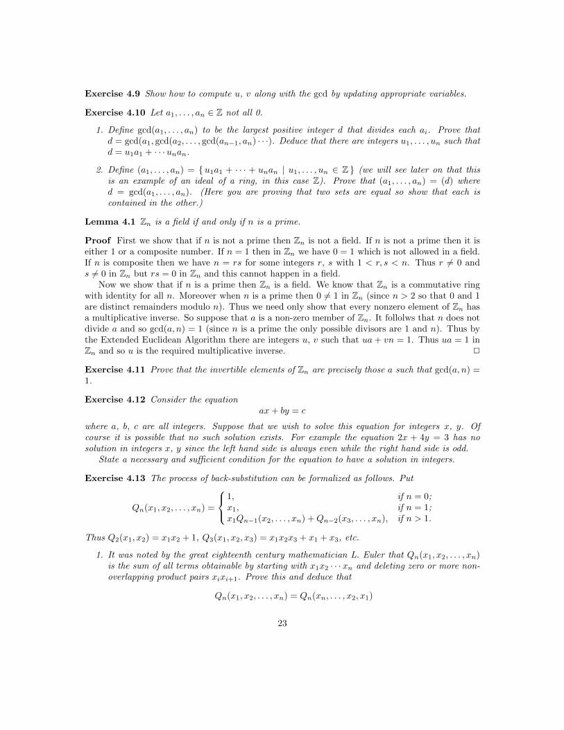
Exercise 4.9 Show how to compute u, v along with the gcd by updating appropriate variables.

Exercise 4.10 Let a1, . . . , an ∈ Z not all 0.

1. Define gcd(a1, . . . , an) to be the largest positive integer d that divides each ai. Prove thatd = gcd(a1, gcd(a2, . . . , gcd(an−1, an) · · ·). Deduce that there are integers u1, . . . , un such thatd = u1a1 + · · ·unan.

2. Define (a1, . . . , an) = {u1a1 + · · · + unan | u1, . . . , un ∈ Z } (we will see later on that thisis an example of an ideal of a ring, in this case Z). Prove that (a1, . . . , an) = (d) whered = gcd(a1, . . . , an). (Here you are proving that two sets are equal so show that each iscontained in the other.)

Lemma 4.1 Zn is a field if and only if n is a prime.

Proof First we show that if n is not a prime then Zn is not a field. If n is not a prime then it iseither 1 or a composite number. If n = 1 then in Zn we have 0 = 1 which is not allowed in a field.If n is composite then we have n = rs for some integers r, s with 1 < r, s < n. Thus r 6= 0 ands 6= 0 in Zn but rs = 0 in Zn and this cannot happen in a field.

Now we show that if n is a prime then Zn is a field. We know that Zn is a commutative ringwith identity for all n. Moreover when n is a prime then 0 6= 1 in Zn (since n > 2 so that 0 and 1are distinct remainders modulo n). Thus we need only show that every nonzero element of Zn hasa multiplicative inverse. So suppose that a is a non-zero member of Zn. It follolws that n does notdivide a and so gcd(a, n) = 1 (since n is a prime the only possible divisors are 1 and n). Thus bythe Extended Euclidean Algorithm there are integers u, v such that ua+ vn = 1. Thus ua = 1 inZn and so u is the required multiplicative inverse. 2

Exercise 4.11 Prove that the invertible elements of Zn are precisely those a such that gcd(a, n) =1.

Exercise 4.12 Consider the equationax+ by = c

where a, b, c are all integers. Suppose that we wish to solve this equation for integers x, y. Ofcourse it is possible that no such solution exists. For example the equation 2x + 4y = 3 has nosolution in integers x, y since the left hand side is always even while the right hand side is odd.

State a necessary and sufficient condition for the equation to have a solution in integers.

Exercise 4.13 The process of back-substitution can be formalized as follows. Put

Qn(x1, x2, . . . , xn) =

1, if n = 0;x1, if n = 1;x1Qn−1(x2, . . . , xn) +Qn−2(x3, . . . , xn), if n > 1.

Thus Q2(x1, x2) = x1x2 + 1, Q3(x1, x2, x3) = x1x2x3 + x1 + x3, etc.

1. It was noted by the great eighteenth century mathematician L. Euler that Qn(x1, x2, . . . , xn)is the sum of all terms obtainable by starting with x1x2 · · ·xn and deleting zero or more non-overlapping product pairs xixi+1. Prove this and deduce that

Qn(x1, x2, . . . , xn) = Qn(xn, . . . , x2, x1)

23

so that for n > 1

Qn(x1, x2, . . . , xn) = xnQn−1(x1, . . . , xn−1) +Qn−2(x1, . . . , xn−2)

2. Prove, by induction on n, that

rn = (−1)n(Qn−2(q2, . . . , qn−1)r0 −Qn−1(q1, . . . , qn−1)r1

)for all n ≥ 2. (Here the qi are the quotients of Euclid’s algorithm applied to r0, r1 and the riare the remainders.)

3. Express Qn(q1, . . . , qn) and Qn−1(q2, . . . , qn) in terms of a, b and gcd(a, b)

Exercise 4.14 Let /x1, x2, . . . , xn/ denote the continued fraction

1

x1 +1

x2 +1

. . .

xn−1 +1

xn

Show thatb

a= /q1, q2, . . . , qn/

where the qi are all the quotients obtained by applying Euclid’s algorithm with r0 = a, r1 = b, e.g.,15/39 = /2, 1, 1, 2/.

(Can you see the relationship between the continued fraction and the polynomials Qi defined inthe preceding exercise?)

See Knuth [39] for more material related to the last two exercises (and Euclid’s algorithm ingeneral).

4.6.2 Worst-Case Runtime of Euclid’s Algorithm

Suppose we carry out Euclid’s algorithm with r0 = a, r1 = b. It is clear that all numbers involvedare no larger than max(a, b) so that we never have to carry out any arithmetic on numbers that arebigger than max(a, b). It follows that if we know the worst possible number of steps of the form

ri = qi+1ri+1 + ri+2

then we shall have a good idea of the worst-case runtime of Euclid’s algorithm. To be precise the ithstep involves us in computing qi+1 and ri+2 which consists of an integer division and a remainder.We shall give an outline of the analysis, which turns out to be a little surprising.

Let F0, F1, F2, . . . denote the Fibonacci sequence defined by

Fn =

{ 0 if n = 0,1 if n = 1,Fn−1 + Fn−2 otherwise.

24

i.e., the sequence 0, 1, 1, 2, 3, 5, . . .. These numbers have many interesting properties, e.g.,

gcd(Fm, Fn) = Fgcd(m,n).

Now suppose we apply Euclid’s algorithm to Fn+2, Fn+1. We observe the following behaviour

Fn+2 = 1× Fn+1 + Fn

Fn+1 = 1× Fn + Fn−1

...

5 = 1× 3 + 2

3 = 1× 2 + 1

2 = 2× 1

and there are exactly n steps. Note how the quotients are all 1 except for the last one which is 2(the last quotient can never be 1 in any application of Euclid’s algorithm with r0 6= r1, can you seewhy?). In other words we are making as little progress as is possible. The following result confirmsan obvious conjecture.

Theorem 4.3 (G. Lame, 1845) For n ≥ 1, let a, b be integers with a > b > 0 such that Euclid’salgorithm applied to a, b requires exactly n steps and such that a is as small as possible satisfyingthese conditions. Then

a = Fn+2, b = Fn+1.

Corollary 4.1 If 0 ≤ a, b < N , where N is an integer, then the number of steps required by Euclid’salgorithm when it is applied to a, b is at most dlogφ(

√5N)e − 2 where φ = 1

2 (1 +√

5), the so-calledgolden ratio.

Proof Let n be the number of steps taken by Euclid’s algorithm applied to a, b. Note that theworst possibility is to have a < b since then the first step is ‘wasted’ in swapping a and b. Thealgorithm then proceeds as though it had been applied to b, a where b > a and takes n − 1 steps.Now according to the theorem we have a = Fn, b = Fn+1. So we want to find the largest n thatsatisfies

Fn+1 < N (2)

Now it can be shown that

Fn =1√5

(φn − φn) (3)

where φ = 1 − φ = 12 (1 −

√5) (see Exercise 4.15 or §4.7.2). Note that φ = −0.6183 . . . and φn

approaches 0 very rapidly. In fact φn/√

5 is always small enough so that

Fn+1 =φn+1

√5

rounded to the nearest integer.

Combining this with equation (2) we obtain n+ 1 < logφ(√

5N) which completes the proof. 2

It is worth noting that logφ(√

5N) is approximately 4.785 log10N + 1.672. For more details seeKnuth [39] or Cormen, Leiserson and Rivest [18].

25

Exercise 4.15 Let

F =

(1 11 0

).

1. Show, by induction on n, that

Fn =

(Fn+1 FnFn Fn−1

)for all n > 0.

2. Find a matrix S such that

SFS−1 =

(λ1 00 λ2

)for some real numbers λ1, λ2. Note that

(SFS−1)n = S−1FnS,(λ1 00 λ2

)n=

(λn1 00 λn2

).

Use these two facts to deduce the formula (3).

4.7 Polynomials

We start by giving a fairly formal definition of polynomials. This will be helpful in understandingthe symbolic nature of Computer Algebra systems. (We have already used polynomials informallyand it is very likely that you are familiar with them. Rest assured that this section simply givesone way of defining them. However there is a widespread misconception about polynomials—see§4.7.1—so take care!)

Let R be a commutative ring with identity, for us it will usually be one of Z, Q, R, C or Zn.Let x be a new symbol (i.e., x does not appear in R). Then a polynomial in the indeterminate xwith coefficients from R is an object of form

a0 + a1x+ a2x2 + · · ·+ anx

n + · · ·

where each ai ∈ R and all but finitely many of the ai are 0. Note that the + which appears abovedoes not denote addition in R (after all x is not an element of R). Indeed we could just regardpolynomials as infinite tuples

(a0, a1, a2, . . .)

but the first notation is much more convenient as we shall see4. We call a0 the constant term ofthe polynomial and ai the coefficient of xi (we regard a0 as the coefficient of x0). The set of allsuch polynomials is denoted by R[x].

4If you are curious here is bit more detail about the connection between the the two approaches. We defineoperations on the sequence notation that give us a ring. We then denote the sequence (0, 1, 0, 0, . . .) by x. From thedefinition of multiplication it follows that xi = (0, . . . , 0, 1, 0, . . .) where the 1 is in position i. From the definitionswe also have that (0, . . . , 0, a, 0, . . .) = a(0, . . . , 0, 1, 0, . . .) = axi. Addition is component-wise and so it follows that(a0, a1, a2, . . .) = a0 + a1x + a2x2 + · · · , so we have now got back to our familiar notation. Strictly speaking thisapproach is much more sound as it uses standard notions and then justifies the new notation.

26

A convenient abbreviation is the familiar sigma notation

∞∑i=0

aixi = a0 + a1x+ a2x

2 + · · ·+ anxn + · · ·

Two polynomials are equal if and only if the coefficients of corresponding powers of x are equal aselements of R. Thus

∞∑i=0

aixi =

∞∑i=0

bixi

if and only if a0 = b0, a1 = b1, a2 = b2 etc. When writing polynomials we normally leave out anyterms whose coefficient is 0. Thus we write

2 + 5x3 − 3x5

rather than2 + 0x+ 0x2 + 5x3 + 0x4 − 3x5 + 0x6 + · · ·

Moreover we can also denote the same polynomial by 5x3 − 3x5 + 2 or by −3x5 + 5x3 + 2. Thus ifai = 0 for all i > 0 then we denote the polynomial by just a0 (such a polynomial is called constant).The zero polynomial has 0 for all of its coefficients and is denoted by 0.

The highest power of x that has a non-zero coefficient in a polynomial p, is called the degreeof p and is denoted by deg(p). The corresponding coefficient is called the leading coefficient of pand is sometimes denoted by lc(p). (These notions do not make sense for the zero polynomial. Weleave deg(0) and lc(0) undefined. For example

deg(x+ 3x3 − 6x10) = 10,

lc(x+ 3x3 − 6x10) = −6.

We define the sum, difference and product of polynomials in the obvious way.

∞∑i=0

aixi ±

∞∑i=0

bixi =

∞∑i=0

(ai ± bi)xi,

( ∞∑i=0

aixi

)( ∞∑i=0

bixi

)=

∞∑i=0

i∑j=0

ajbi−j

xi.

If m, n are the respective degrees of the two polynomials then we can write these definitions as

m∑i=0

aixi ±

n∑i=0

bixi =

max(m,n)∑i=0

(ai ± bi)xi,

(m∑i=0

aixi

)(n∑i=0

bixi

)=

m+n∑i=0

i∑j=0

ajbi−j

xi

where it is understood that ai is 0 if i > m and similarly bj is 0 if j > n. Note that the definitionabove yields ax = xa for all a ∈ R from which it follows that every element of R commutes with

27

every polynomial. It is quite easy to show that, with these definitions, the three operations onpolynomials obey various well known (and usually tacitly assumed) rules of arithmetic such as

p+ q = q + p,

pq = qp,

(p+ q) + r = p+ (q + r),

(pq)r = p(qr),

p(q + r) = pq + pr.

Indeed R[x] is a commutative ring with identity under the operations given above. We have

deg(p± q) ≤ max(

deg(p),deg(q)),

deg(pq) ≤ deg(p) + deg(q),

deg(pq) = deg(p) + deg(q), if lc(p) lc(q) 6= 0,

whenever both sides are defined. For example

(2 + 3x− 4x3) + (−3x+ 2x2) = (2 + 0) + (3− 3)x+ (0 + 2)x2 + (−4 + 0)x3

= 2 + 2x2 − 4x3

while

(2 + 3x− 4x3)× (−3x+ 2x2) = (2 · 0)

+ (2 · (−3) + 3 · 0)x

+ (2 · 2 + 3 · (−3) + 0 · 0)x2

+ (2 · 0 + 3 · 2 + 0 · (−3) + (−4) · 0)x3

+ (2 · 0 + 3 · 0 + 0 · 2 + (−4) · (−3) + 0 · 0)x4

+ (2 · 0 + 3 · 0 + 0 · 0 + (−4) · 2 + 0 · (−3) + 0 · 0)x5

= −6x− 5x2 + 6x3 + 12x4 − 8x5.

If the coefficients come from Z then the degree of the product is equal to the sum of the degrees.On the other hand if the coefficients come from Z8 then the product polynomial is equal to 2x +3x2 + 6x3 + 4x4 and the degree of the product is less than the sum of the degrees of the two factors.

The preceding example makes rather heavy weather of the process of multiplying polynomials.An alternative approach is to multiply each term of the first polynomial with each one of the secondand then collect coefficients of equal powers of x. we can write this out in tabular form as follows

2 + 3x − 4x3

− 3x + 2x2

− 6x − 9x2 + 12x4

+ 4x2 + 6x3 − 8x5

− 6x − 5x2 + 6x3 + 12x4 − 8x5

28

Of course this is just the same process as the familiar school method of multiplying integers, withthe difference that we do not need to concern ourselves with carries. Most computer algebrasystems multiply polynomials by an algorithm based on this process. (It is interesting that theimplementation of such a simple algorithm still presents a subtlety about the amount of memoryused—see [21], p. 66.)

4.7.1 Polynomial Functions

Given a polynomialp = a0 + a1x+ · · ·+ anx

n

we can define a corresponding function p : R→ R by putting

p(α) = a0 + a1α+ · · ·+ anαn

for each α ∈ R. The preceding expression looks so much like the polynomial p that it is commonpractice to identify the function and the polynomial (indeed the indeterminate x is frequentlyreferred to as a variable). This is potentially dangerous since, e.g., the notions of equality betweenpolynomials and between functions are completely different. Recall that two functions f, g : R→ Rare said to be equal if and only if f(α) = g(α) for all α ∈ R. Now let p be as above and

q = b0 + b1x+ · · ·+ bmxm.

We have thatp = q ⇔ ai = bi, for i = 0, 1, . . .

⇔ p = q = 0, or

deg(p) = deg(q) & ai = bi, for 0 ≤ i ≤ deg(p).

On the other hand if we think of p and q as functions (i.e., identify them with p and q) then wehave

p = q ⇔ p(α) = q(α) for all α ∈ R.

Fortunately as long as R is an infinite integral domain (such as Z or any field) then it can be shownthat the two definitions coincide and so there is no harm in confusing the polynomial p with thecorresponding function p. (In fact there is a deeper reason, the ring of polynomial functions isisomorphic to the ring of polynomials.)

Exercise 4.16 Let p be a polynomial with coefficients from an integral domain R. A number α issaid to be a root of p if p(α) = 0. It can be shown that if p 6= 0 then it has at most deg(p) rootsin R. Use this fact to show that p = q if and only if p = q for two polynomials p and q when R isinfinite.

When R is finite the situation is completely different. Let the elements of R be r1, . . . , rn and put

Z(x) = (x− r1) · · · (x− rn).

Assume that n > 1 so that 1 6= 0 in R. Then clearly Z(x) is not the zero polynomial (it has degree nand leading coefficient 1). However the associated polynomial function Z is the zero function.

29

Exercise 4.17 This exercise shows that if R is not an integral domain then the distinction betweenpolynomials and the corresponding functions is important even if R is infinite.

Let R1, R2 be two commutative rings with identities 1A and 1B respectively. Show that theobvious definitions turn

R1 ×R2 = { (r1, r2) | r1 ∈ R1, r2 ∈ R2 }

into a ring with identity (1A, 1B) and zero (0A, 0B). Now let a = (1A, 0B) and deduce that everyelement of the form (0A, r2) is a root of the polynomial ax.

4.7.2 Digression: Formal Power Series

Another way of defining polynomials is as finite expressions of the form

n∑i=0

aixi.

We can proceed with our definitions as before.The definition via infinite tuples suggests a possible generalization: drop the condition that all

but finitely many of the coefficients must be 0. All the definitions go through exactly as beforeand we thus obtain the ring R[[x]] of formal power series in the indeterminate x with coefficientsfrom R. Notice that here there is no question of worrying about convergence. This matter onlyarises when we wish to consider a formal power series P (x) as a function R → R just as in thecase of polynomial functions. Clearly every polynomial is a formal power series and indeed the ringof polynomials R[x] is a subring of R[[x]]. Algebraically speaking we make quite a gain in movingfrom R[x] to R[[x]]. For example in R[x] an element p has a multiplicative inverse (i.e., there is a qsuch that pq = 1) if and only if p is a constant (i.e., an element of R) and has an inverse in R. Theonly invertible polynomials in Z[x] are 1 and −1. However in the ring of formal power series R[[x]]it is easy to see that an element P has a multiplicative inverse if and only if its constant term (i.e.the coefficient of x0) is non-zero and has an inverse in R—the other coefficients can be arbitrary.For example in Z[[x]] we have

(1− x)(1 + x+ x2 + x3 + · · ·+ xn + · · ·) = 1

so that1

1− x= 1 + x+ x2 + x3 + · · ·+ xn + · · ·

(It is common practice to use 1/a to denote the inverse of an invertible element of a ring R.) Theseideas are very useful in many areas; we give an illustration from enumerative combinatorics. Leta0, a1, . . . be a sequence of numbers. We define the generating function of this sequence by

A(x) = a0 + a1x+ a2x2 + · · ·

(although A(x) is called a generating function this is just a nod to tradition and it is really a formalpower series). To illustrate the usefulness of this notion let us consider our old friends the Fibonaccinumbers F0, F1, F2, . . .. The generating function for these is

F (x) = F0 + F1x+ F2x2 + · · ·

30

Now it is clear thatF (x)(1− x− x2) = x

and this is true in R[[x]]. Moreover 1−x−x2 has a non-zero constant term and so it has an inversein R[[x]]. Thus

F (x) =x

1− x− x2

=−x

(φ+ x)(φ+ x)

where φ = 12 (1 +

√5) and φ = 1

2 (1 −√

5) (of course −φ and −φ are the two roots of 1 − x − x2).Thus, from the partial fraction decomposition of the last expression, we have

F (x) =x√5

(1

φ+ x− 1

φ+ x

).

It is clear that φφ = −1 and so

1

φ+ x=−φ

1− φx= −φ(1 + φx+ (φx)2 + · · ·)= −φ− φ2x− φ3x2 − · · ·

and similarly

1

φ+ x=−φ

1− φx= −φ− φ2x− φ3x2 − · · · .

Thus

F (x) =x√5

(1

φ+ x− 1

φ+ x

)=

1√5

(φ− φ)x+1√5

(φ2 − φ2)x2 +1√5

(φ3 − φ3)x3 + · · · .

Equating coefficients we obtain

Fn =1√5

(φn − φn)

=1√5

((1 +√

5

2

)n−

(1−√

5

2

)n).

4.7.3 Polynomials in Several Indeterminates

Since R[x] is a commutative ring with identity we can repeat the whole polynomial ring constructionwith a new indeterminate y to obtain a new ring R[x][y] of polynomials in y with coefficients fromR[x]. Every element of R[x][y] can be written in the form

∞∑i,j=0

rijxiyj (4)

31

where rij ∈ R for all i, j. This helps to reveal the fact that R[x][y] and R[y][x] are essentially thesame ring (i.e. they are isomorphic). Because of this we use the notation R[x, y]. (Note that that x,y commute, i.e., xy = yx.) When taking this latter view each product xiyj in (4) is called a powerproduct in x, y of degree i+ j. Thus in this view the degree of (4) is undefined if all coefficients rijare 0 and otherwise it is the maximum degree of a power product which occurs in it with non-zerocoefficient. The properties of degrees given above carry through to the new situation. We use aphrase such as ‘degree in x’ to indicate that we are viewing a polynomial of R[x, y] as being in theindeterminate x with coefficients from R[y], this degree is denoted by degx(·). Similar commentsapply to the leading coefficient, which is defined when we are focusing on one indeterminate as the‘main’ one. For example

deg(1 + x+ x2y + x3y + 2x3y2) = 5 lc not defined

degx(1 + x+ x2y + x3y + 2x3y2) = 3 lcx(1 + x+ x2y + x3y + 2x3y2) = y + 2y2

degy(1 + x+ x2y + x3y + 2x3y2) = 2 lcy(1 + x+ x2y + x3y + 2x3y2) = 2x3

The concept of leading coefficient does not make sense when we consider polynomials in severalindeterminates at once because then there are usually several different power products of the same(highest) degree. Consider for example the polynomial

x3 + x2y + xy2 + y3 + xy + x+ y + 1.

This has degree 3 and has four power products of this degree. In order to give a meaning tothe concept of leading coefficient we must have some notion of one power product being moreimportant than another, i.e., we must introduce a total order on power products. This is a veryuseful idea and we will discuss it later on when considering representations of polynomials as well asthe construction of Grobner bases. Of course if we specify a power product t then it always makessense to ask for its coefficient, which could be 0, in a polynomial p. This is denoted by coeff(t, p).

Clearly we can generalize polynomial rings to finite sets X = {x1, . . . , xn} of indeterminates.The power products here are all expressions of the form

xi11 · · ·xinnwhere i1, . . . , in ∈ N. The degree of such a power product is just i1 + · · ·+ in. Finally an expressionof the form ct where c ∈ R and t is a power product is called a monomial.

4.7.4 Differentiation

Letp = a0 + a1x+ · · ·+ anx

n

be a polynomial in x with coefficients from some commutative ring R. Then we can define itsderivative in a purely formal manner as

p′ = a1 + 2a2x+ · · ·+ nanxn−1.

(We sometimes use the traditional notation dp/dx instead of p′.) Note that there is no reliance onlimits here. It is easy to see that all the algebraic properties of derivatives (i.e., ones that do notdepend on limits) still hold. Thus

(p+ q)′ = p′ + q′

(pq)′ = p′q + pq′.

32

It follows from the definition that p′ = 0 if p ∈ R. However the converse is not necessarily true:consider x2 + 1 ∈ Z2[x]. Of course the converse is true when the coefficients come from the familiarnumber systems Z, Q, R or C.

Let k be any field and k(x) consist of all ratios p/q where p, q ∈ k[x] and q 6= 0. If we defineaddition and multiplication in the obvious way then k(x) is a field (see §4.7.8). We can extend thedefinition of differentiation to k(x) by putting

(p/q)′ =p′q − pq′

q2,

where p, q ∈ k[x]. We can also define partial derivatives (e.g., for elements of k(x, y)) in the obviousway.

Exercise 4.18 Let f be an element of Zp[x] where p is a prime number. Show that f ′ = 0 if andonly if f ∈ Zp[xp] i.e., f has the form

f = a0 + a1xp + a2x

2p + · · ·+ anxpn.

4.7.5 Factorization and Greatest Common Divisors

Let R be a unique factorization domain (UFD), which for the moment can be interpreted as Z, orany field (normally Q or Zp for p a prime). The first important consequence of this assumption isthat

deg(pq) = deg(p) + deg(q), for all p, q ∈ R[x].

We know that in R we can factorize non-zero elements into primes, can we extend this to polynomialsfrom R[x]? Given an arbitrary (non-zero) polynomial p we can try to write it as a product p = hkwhere h, k have degree which is strictly smaller than that of p (this means that they cannot beconstant polynomials). If this is possible then we can repeat the process with h and k and so on.This process must eventually stop because at each stage the degree of the relevant polynomialsdecreases and of course it is always greater than 0. Thus we have

p = p1p2 · · · ps.

where each pi cannot be expressed as a product of two polynomials of smaller degree. We shouldlike this factorization to be unique in the same sense that the factorization of numbers into primesis unique. Consider however the factorizations

6x2 + 30x+ 36 = (2x+ 4)(3x+ 9)

= 2 · 3(x+ 2)(x+ 3)

where the polynomials are from Z[x]. None of the factors is invertible in Z[x] but the number offactors in the two factorizations is different. The source of the problem is obvious: in the firstfactorization the polynomials 2x + 4 and 3x + 9 are not irreducible elements of the ID Z[x]. Inother words the process which we described did not carry out a complete factorization. (This kindof difficulty does not arise when R is a field—can you see why?) Now given

f = a0 + a1x+ · · ·+ anxn

33

define the content of f , denoted by cont(f), to be the gcd of its coefficients. If the content of f is cthen we may write

f = cg

and call g the primitive part of f , denoted by pp(f). (A polynomial is called primitive if its contentis 1 or any invertible element.) In order to obtain a unique factorization for p we write each pi ascip′i where ci is the content of pi. We may then collect all the contents together into one element c

of R and putp = cp′1p

′2 · · · p′s.

Suppose that we also havep = dq1q2 · · · qt,

where each qi is primitive and cannot be written as the product of two polynomials of lower degree.Then it is a remarkable fact that:

1. d = εc for some invertible element ε of R,

2. s = t, and

3. there is a permutation π of 1, 2, 3, . . . , s such that p′i = εiqπ(i) for 1 ≤ i ≤ n where each εi isan invertible element of R.

In other words R[x] is a UFD. (Why do we not bother factorizing c and d?)What we have is that if R is a UFD then so is R[x]. Thus if R is a UFD then so is R[x, y]

because we can regard this as R[x][y] and let R[x] play the role of R in the preceding discussion.It is now clear that the same can be said of R[x1, . . . , xn].

Naturally there is a huge difference between knowing that polynomials can be factorized andactually producing a factorization. This is one important application area of Computer Algebra.

It is worth noting that the phrase irreducible polynomial is normally used in the following sense: pis said to be irreducible if we cannot write it as the product of two other polynomials of smallerdegree. Thus 2x+4 is an irreducible polynomial of Z[x] even though it is not an irreducible elementof this ring! As another example x2 + 1 is irreducible as a polynomial in R[x]. To see this supposeotherwise, then we must have

x2 + 1 = (a1x+ a0)(b1x+ b0)

for some real numbers a0, a1, b0, b1. Note that a1 6= 0 otherwise the degree of the right hand side istwo low. But now this means that −a0/a1 is a root of x2 + 1 and this is impossible since the squareof any real number is non-negative. This example brings out a very important fact: the conceptof irreducibility depends on the ring R of coefficients. If we regard x2 + 1 as a polynomial in C[x]then of course we can factorize it as (x+ i)(x− i) where i =

√−1.

Exercise 4.19 Prove that x2 − 2 is irreducible in Z[x] but of course in R[x] it factorises.

We now turn our attention to the gcd and assume that f 6= 0 or g 6= 0 so any gcd is non-zero.Recall from §4.2 that h is a gcd of two polynomials f , g if h divides both of the polynomials andany other common divisor of f , g also divides h. Furthermore any two gcd’s are related by aninvertible element, which in the case of polynomial rings must be an invertible constant from thering of coefficients R (prove this). It is easy to see that no polynomial of degree strictly larger thanthat of h can be a common divisor of f , g. If R is a field then all nonzero constants are invertible

34

and this means that we can define gcd’s of f , g to be all those common divisors of f , g of largestpossible degree. If R is not a field then this is not quite enough to capture the gcd (we mightbe missing some constant non-invertible factor). It is standard practice to abuse notation and usegcd(f, g) to stand for a greatest common divisor of f , g and even talk of the gcd. This does noharm because we are not normally bothered about multiples by invertible elements. In many casesit is possible to remove the ambiguity by insisting on some extra condition that must be satisfiedby a gcd. For example if the coefficients are rationals then we can insist that the leading coefficientshould be 1 (i.e., the gcd is monic).

Just as in the case of the integers there is a very close connection between the gcd and factor-ization. It is left up to you to work this out if you are interested.

We will also make use of the least common multiple of two polynomials f , g. This is a polynomialof least possible degree which is divisible by both f and g. It is unique up to constant factors andis denoted by lcm(f, g). In fact we have lcm(f, g) = fg/ gcd(f, g).

4.7.6 Euclid’s Algorithm for Univariate Polynomials

Let f , g be univariate polynomials with coefficients from a field. Suppose we wish to find gcd(f, g)where g 6= 0 and we have

f = qg + r (5)

where r = 0 or deg(r) < deg(g). We call q the quotient of f divided by g and r the remainder. Nowif h | f and h | g then certainly h | r. On the other hand if h | g and h | r then h | f . It follows fromthis that gcd(f, g) is the same as gcd(g, r). For the moment we assume that we can always find anexpression of the form (5). This means that we can find polynomial gcd’s by mimicking Euclid’salgorithm for integer gcd’s. To be specific we put r0 = f , r1 = g and

r0 = q1r1 + r2

r1 = q2r2 + r3

r2 = q3r3 + r4

...

rs−2 = qs−1rs−1 + rs

rs−1 = qsrs + rs+1

where rs+1 = 0 and deg(ri) < deg(ri−1) for 1 ≤ i ≤ s. Note that we must eventually have ri = 0for some i since deg(r0) > deg(r1) > . . . > deg(ri) > . . . ≥ 0.

Let us now see how to find q, r so that (5) holds. If f = 0 then we just take q = 0, r = 0.Otherwise we could try q = 0, r = f . This is fine unless deg(f) ≥ deg(g); however if this is so thenwe can improve matters by (repeatedly) replacing q with q+(a/b)xm−n and r with r− (a/b)xm−ngwhere a = lc(r), b = lc(g), m = deg(r) and n = deg(g). Each time this is done the degree of rdrops and so we must eventually have r = 0 or deg(r) < deg(g) as required. The correctness of themethod follows from the loop invariant qg + r = f (check this).

Note that we can calculate the quotient and remainder polynomials by hand in a manner similar

35

to the long division of integers. For example we can divide x3−x2 +x−1 by x2−2x+ 1 as follows:

x + 1

x2 − 2x + 1 x3 − x2 + x − 1

x3 − 2x2 + x

x2 − 1

x2 − 2x + 1

2x − 2

The quotient is x + 1 and the remainder is 2x − 2. Here we were lucky in that no fractions wereneeded, in general the calculations involve fractions even if the inputs have integer coefficients.

We now focus on polynomials with rational coefficients. Note that the Euclidean Algorithm reliesquite heavily on rational arithmetic and this can be quite costly due to the many gcd computations(on coefficients) carried out. We could avoid this by clearing denominators from the inputs. We mayalso use the fact that if f , g are non-zero polynomials with integer coefficients and deg(f) ≥ deg(g)then we can find polynomials q, r with integer coefficients such that

lc(g)deg(f)−deg(g)+1f = qg + r

where r = 0 or deg(r) < deg(g). This leads to an obvious modification of Euclid’s algorithm.Unfortunately this process can lead to very large integers even when the input consists of smallones. For example consider

f = x8 + x6 − 3x4 − 3x3 + 8x2 + 2x− 5,

g = 3x6 + 5x4 − 4x2 − 9x+ 21.

The sequence of remainders obtained by applying the modified algorithm is

−15x4 + 3x2 − 9,

15795x2 + 30375x− 59535,

1254542875143750x− 1654608338437500,

12593338795500743100931141992187500.

(Collectors of obscure misprints will be interested to learn that the final 4 in the last remainderis given as a 5 in [21], p. 69.) Obviously we could try to keep the growth of coefficients down byremoving their common factors. Thus

anxn + an−1x

n−1 + · · ·+ a0

could be replaced by(an/d)xn + (an−1/d)xn−1 + · · ·+ (a0/d)

36

whered = gcd(an, an−1, . . . , a0).

But the whole point of avoiding rational arithmetic was because of its need to compute many gcd’s!The excessive growth of the coefficients is clearly caused by the factor lc(g)deg(f)−deg(g)+1 which

enables us to stay with integer arithmetic. In fact this is larger than necessary and it is possibleto construct algorithms, known as sub-resultant polynomial remainder sequences, which avoid thislarge growth. We do not go into details here since we will look at a different method later on whichis the one used in practice.

Finally the discussion in §4.6.1 on the Extended Euclidean Algorithm for the integers carriesover directly to the version for polynomials. We can therefore find polynomials u, v such that

uf + vg = d

where d = gcd(f, g). Moreover we can ensure that u = 0 or deg(u) < deg(g) and v = 0 ordeg(v) < deg(f).

Exercise 4.20 Consider equations of the form

fY + gZ = h

where f , g and h are polynomials in x and Y , Z are unknowns. Find a a necessary and sufficientcondition for such an equation to have solutions in X, Y that are themselves polynomials. Describea method for finding such solutions when they exist.

Exercise 4.21 A naıve attempt at extending Euclid’s algorithm to multivariate polynomials doesnot succeed; why?

4.7.7 A Remainder Theorem

Let p(x) ∈ k[x] be a polynomial in the indeterminate x with coefficients from the field k. Chooseany α ∈ k. Then we have

p(x) = (x− α)q(x) + r(x)

for some q(x), r(x) ∈ k[x] where r(x) = 0 or deg(r) < deg(x− α) = 1 so that r(x) ∈ k, i.e., r(x) isa constant. Indeed if we substitute α for x we see that p(α) = r (we do not write r(α) since r doesnot depend on x). Note that α is a root of p(x) if and only if r = 0, i.e., if and only if x− α | p(x).This fact can be used to show that p(x) has at most deg(p) roots (easy exercise in induction). Wecan summarize the discussion by saying that for all α ∈ k

p(x)− p(α) = (x− α)q(x),

for some q(x) ∈ k[x]. We can prove this directly by showing that

xi = ((x− α) + α)i

= (x− α)qi(x) + αn,

for some qi(x) ∈ k[x]. This is fairly obvious and is easy to prove by induction on i. The full resultfollows from the fact that p(x) is a linear combination of 1, x, x2, . . .. The reason for looking at thisproof is that it readily generalizes to multivariate polynomials. Suppose that f(x1, x2, . . . , xn) ∈

37

k[x1, x2, . . . , xn] and α1, α2, . . . , αn ∈ k. We say that (α1, α2, . . . , αn) is a root of f(x1, x2, . . . , xn)if and only if f(α1, α2, . . . , αn) = 0. Suppose that

f = (x1 − α1)g1 + (x2 − α2)g2 + · · ·+ (xn − αn)gn,

for some g1, g2, . . . , gn ∈ k[x1, x2, . . . , xn]. Then it is clear that (α1, α2, . . . , αn) is a root of f . Infact the converse is true for f is a linear combination of power products xi11 x

i22 · · ·xinn . Now, putting

yi = xi − αi as a notational convenience, we have

xi11 xi22 · · ·xinn = (y1 + α1)i1(y2 + α2)i2 · · · (yn + αn)in

= (y1h1 + αi11 )(y2h2 + αi−22 ) · · · (ynhn + αinn )

where hi ∈ k[xi]. Now it is clear that the final expression, when multiplied out can be collected soas to have the form

y1q1 + y2q2 + · · ·+ ynqn + αi11 αi22 · · ·αinn , (†)

where q1, q2, . . . , qn ∈ k[x1, x2, . . . , xn]. Note that there may be more than one way of collectingterms so there may be more than one choice for the qi. As an example consider x2

1x2 with α1 = 1,α2 = 2 so that y1 = x1 − 1 and y2 = x2 − 2. Then

x21x2 = (y1 + 1)2(y2 + 2)

= y21y2 + 2y2

1 + 2y1y2 + 4y1 + y2 + 2

.

Now the last term can written as

y1(y1y2 + 2y1 + 2y2 + 4) + y2 + 2

or asy1(2y1 + 2y2 + 4) + y2(y2

1 + 1) + 2

as well as many other ways, all of which have the form (†). Now using the fact that f is a linearcombination of power products of the xi we see that

f = y1g1 + y2g2 + · · ·+ yngn + f(α1, α2, . . . , αn)

for some g1, g2, . . . , gn ∈ k[x1, x2, . . . , xn]. Finally we have

f(x1, x2, . . . , xn)− f(α1, α2, . . . , αn) = (x1 − α1)g1 + (x2 − α2)g2 + · · ·+ (xn − αn)gn.

We will use this fact later on when we look at the solution of simultaneous polynomial equations.Before leaving this section it is worth noting that it provides an excellent illustration of a process

that happens quite frequently in Mathematical subjects. We have a result for a special case (herethe remainder theorem for univariate polynomials). This result can be derived quite easily fromEuclid’s Algorithm. However the view implied by this proof does not generalize (Euclid’s Algorithmdoes not hold for multivariate polynomials). However a little more work shows that we can findanother proof that gives us not only another view of the result but also generalizes. Indeed thisprocess of generalization will reach a very impressive level when we look at Grobner bases sincethese can be seen as a generalization of Euclid’s Algorithm to multivariate polynomials.

38

4.7.8 Rational Expressions

Let k be any field. Given the polynomial ring k[x1, . . . , xn] we can form the set

k(x1, . . . , xn) = {p/q | p, q ∈ k[x1, . . . , xn] & q 6= 0}.

Two elements p/q and p′/q′ of k(x1, . . . , xn) are said to be equal if and only if pq′ − p′q = 0 as apolynomial in k[x1, . . . , xn]. We define addition and multiplication by

(p/q) + (p′/q′) = (pq′ + p′q)/qq′,

(p/q)(p′/q′) = pp′/qq′.

(Can you prove that these definitions are unambiguous?) Given these operations k(x1, . . . , xn)becomes a field and is called the field of rational expressions (or rational functions or quolynomials)in x1, . . . , xn over k.

Just as in the case of polynomials it is common practise to regard an expression such as (x2 −1)/(x− 1) as a function. But this can be rather confusing because here the expression x + 1 doesnot denote the same function since the latter is defined at x = 1 while the former is not. (Of coursethe two functions are both defined at all other points and have equal values.) Note however thatas elements of k(x) the two expressions are equal since (x2 − 1) = (x + 1)(x − 1) as polynomials.Computer Algebra systems work with such expressions in the algebraic rather than the functionalsense. Despite this it is common mathematical practice to call such objects rational functions ratherthan rational expressions as we have done. See also [21], pp. 72–74.

4.7.9 Representation of Polynomials and Rational Expressions

First of all we deal with polynomials. We are considering the elements of R[x1, . . . , xn] where R isa ring (for whose elements we have a representation). Representations can be classified as recursiveor distributive either of which may be dense or sparse. This gives us four possibilities, the choicedepends on the application at hand. The most common representation is the recursive sparse onealthough for Grobner bases a distributed sparse one is most useful.

Recursive Representation

This is just an expression of the isomorphism

R[x1, . . . , xn] ∼= R[x1, . . . , xn−1][xn]

and we regard xn as the main indeterminate. For example

f = 3xy2 + 2y2 − 4x2y + y − 1

may be represented as(3x+ 2)y2 + (−4x2 + 1)y + (−1)y0

where y is the main indeterminate. In general we use∑cix

in where the ci are polynomials which

are themselves represented in a similar format. The Axiom type is UP(x,UP(y,INT)) (here andelsewhere INT can be replaced by any integral domain). Note that Axiom prints back the polynomialin expanded form but it is held as indicated as a use of coefficients f shows.

39

Distributive Representation

We consider the power products in the given indeterminates e.g., x21x3x

75. We pick a total order

on the power products such that 1 (which stands for x01 · · ·x0

n) is least and for each power productthere are only finitely many less than it. We may now write a polynomial p(x0, . . . , xn) as

p(x0, . . . , xn) =∑t≤t

ctt

where ct ∈ R for each t. As an example of a suitable order we could first sort according to degreeand within each degree use the lexicographic order: we order the indeterminates, e.g.,

x1 >L x2 >L · · · >L xn

and thenxi11 · · ·xinn >L x

j11 · · ·xjnn

if and only if there is a k such that il = jl for 1 ≤ l < k and ik > jk. This is called the gradedlexicographic order. By contrast if we order power products purely lexicographically then we do nothave a suitable order because there can be infinitely many power products less than a given one(see the example on p. 69). With f as above, the Axiom type is DMP([x,y],INT) (an alternativeis HDMP([x,y],INT) which imposes a different order on power products.

Dense Representations

In a dense representation we record all the coefficients up to the highest degree of the main inde-terminate or the highest power product. Thus for a recursive representation we might have

m∑i=0

cixi ←→ (c0, . . . , cm)

and for a distributed representation∑t≤t

ctt←→ (c1, ct1 , . . . , ct),

where (. . .) denotes a list or array. The problem is that this representation can lead to a great dealof wasted space, e.g., consider x1000 + 1 or x4y7 + x+ 1.

Exercise 4.22 How many power products of degree d are there in the indeterminates x, y? Gen-eralize to power products in n indeterminates.

Sparse Representations

For these we drop all zero coefficients. This means that with each non-zero coefficient we mustrecord the corresponding degree or power product. For example

x1000 + 1←→ ((1, 1000), (1, 0)),

x4y7 + 2x+ 1←→ ((1, (4, 7)), (2, (1, 0)), (1, (0, 0))).

In the second example a power product xe11 · · ·xenn is represented by (e1, . . . , en). In general Axiomuses a sparse representation.

40

Rational Expressions

The obvious representation for these is as a pair of polynomials consisting of the numerator anddenominator. If the numerator is in normal form then we also have a normal form for rationalexpressions (since f/g = 0 iff f = 0, of course we must have g 6= 0 for f/g to be a rationalexpression at all). It is tempting, by analogy with the rational numbers, to remove gcd(f, g)from the numerator and denominator of f/g. However this can be very unwise: for example(1 − xn)/(1 − x) is very compact and requires little storage even for large n. Removing the gcdgives us 1 + x + · · · + xn−1 which is expensive in storage space and clutters up any output in anasty way! The situation becomes even worse when multivariate polynomials are involved. We alsohave to bear in mind that polynomial gcd’s are fairly costly to compute (compared to integer ones).However the default behaviour of Axiom is to take out the gcd, by contrast Maple does not.

Exercise 4.23 Consider rational expressions in one indeterminate and rational coefficients. Evenif we remove the gcd from the numerator and denominator we still do not have a canonical form.Give a method that leads to a canonical form which uses only integer coefficients. (Here we assumethat integers are held in a canonical form, which is always the case.)

Intermediate Expression Swell

We know from §4.7.6 that computing the gcd of

A = x8 + x6 − 3x4 − 3x3 + 8x2 + 2x− 5,

B = 3x6 + 5x4 − 4x2 − 9x+ 21,

using Euclid’s algorithm over the integers leads to rather large integers, even though the inputand output are small (we are justified in claiming that the output is small because any non-zeronumber, e.g., 1, is a valid answer, remember that we are working with coefficients over Q). Thisphenomenon of intermediate expression swell is such a major problem in computer algebra that itis worth seeing another example of it.

Some systems (e.g., Maple) use a sum of products representation for polynomials (and otherexpressions). In this representation we take a sum over products of polynomials rather than justa sum over monomials. This representation is compact but it does mean that we cannot tell justby looking at it whether or not a given representation yields the zero polynomial. In order toachieve this it appears that we must expand terms—at least nobody knows of any way round this.Unfortunately this process can lead to an exponential increase in the number of terms produced. Thefollowing is an example of this. The Vandermonde determinant of n indeterminates x1, x2, . . . , xnis defined by:

V (x1, x2, . . . , xn) =

∣∣∣∣∣∣∣∣∣∣

1 1 . . . 1x1 x2 . . . xnx2

1 x22 . . . x2

n...

......

xn−11 xn−1

2 . . . xn−1n

∣∣∣∣∣∣∣∣∣∣.

It can be shown thatV (x1, x2, . . . , xn) =

∏1≤i<j≤n

(xj − xi).

41

(Thus V (x1, x2, . . . , xn) = 0 if and only if xi = xj for some i 6= j.) Now put

Z(x1, x2, . . . , xn+1) =

∣∣∣∣∣∣∣∣∣∣∣∣∣

1 1 . . . 11 1 . . . 1x1 x2 . . . xn+1

x21 x2

2 . . . x2n+1

......

...xn−1

1 xn−12 . . . xn−1

n+1

∣∣∣∣∣∣∣∣∣∣∣∣∣.

This is 0 since the first two rows are equal. However expanding along the first row we have

Z(x1, x2, . . . , xn+1) =

n+1∑i=1

(−1)i+1V (x1, . . . , xi, . . . , xn+1)

=

n+1∑i=1

(−1)i+1∏

1≤j<k≤n+1j,k 6=i

(xk − xj),

where x1, . . . , xi, . . . , xn+1 denotes the sequence x1, x2, . . . , xn+1 with xi deleted. Now the lastexpression is a perfectly good sum of products representation but any attempt at expanding itleads to n! terms for each summand and cancellation takes place only between summands!

We therefore have a difficult choice: systems that expand automatically will face a huge penaltyat some point. Systems that do not expand automatically leave open the possibility of undetecteddivisions by 0 and the user must look out for such difficulties. The next exercise shows a probabilisticapproach to deciding equality to 0 without expanding.

Exercise 4.24 Let p(x1, x2, . . . , xn) be a non-zero polynomial with coefficients from Q and put

V(p) = { (a1, a2, . . . , an) ∈ Qn | p(a1, a2, . . . , an) = 0 }.

It is a fact that if we pick the ai randomly (from some range) then the probability that we obtain amember of V(p) (i.e., a root of p) is 0. (Think of algebraic curves in 2 dimensions and surfaces in3 dimensions.) Can you use this to develop a fast randomized test for a polynomial expression beingzero? To be more precise if the test tells us that the polynomial is non-zero then the answer mustbe correct. If on the other hand the test tells us that the polynomial is zero then the answer mustbe correct with high probability. (See J. T. Schwartz, Fast Probabilistic Algorithms for Verificationof Polynomial Identities, J. ACM, 27, 4, (1980) 701–717.)

42