Introduction to Computational Quantum Chemistry:...
101
Introduction to Computational Quantum Chemistry: Theory Dr Andrew Gilbert Rm 118, Craig Building, RSC 3108 Course Lectures 2007
Transcript of Introduction to Computational Quantum Chemistry:...

Introduction to Computational QuantumChemistry: Theory
Dr Andrew Gilbert
Rm 118, Craig Building, RSC
3108 Course Lectures 2007

Introduction Hartree–Fock Theory Configuration Interaction
Lectures
1 IntroductionBackgroundThe wave equationComputing chemistry
2 Hartree–Fock TheoryThe molecular orbital approximationThe self-consistent fieldRestricted and unrestricted HF theory
3 Configuration InteractionThe correlation energyConfiguration expansion of the wavefunction

Introduction Hartree–Fock Theory Configuration Interaction
Lectures
4 Correlated MethodsConfiguration interactionCoupled-cluster theoryPerturbation theoryComputational Cost
5 Basis SetsBasis functionsAdditional types of functions
6 Density Functional TheoryDensity functionalsThe Hohenberg–Kohn theoremsDFT models

Introduction Hartree–Fock Theory Configuration Interaction
Lectures
7 Model ChemistriesModel chemistries

Introduction Hartree–Fock Theory Configuration Interaction
Lecture
1 IntroductionBackgroundThe wave equationComputing chemistry
2 Hartree–Fock TheoryThe molecular orbital approximationThe self-consistent fieldRestricted and unrestricted HF theory
3 Configuration InteractionThe correlation energyConfiguration expansion of the wavefunction

Introduction Hartree–Fock Theory Configuration Interaction
Background
Computational chemistry
Computational Chemistry can be described as chemistryperformed using computers rather than chemicals.It covers a broad range of topics including:
CheminformaticsStatistical mechanicsMolecular mechanicsSemi-empirical methodsAb initio quantum chemistry
All these methods, except the last, rely on empiricalinformation (parameters, energy levels etc.).
In this course we will focus on the last of these methods.

Introduction Hartree–Fock Theory Configuration Interaction
Background
Ab initio quantum chemistry
Ab initio means “from the beginning” or “from firstprinciples”.
Ab initio quantum chemistry distinguishes itself from othercomputational methods in that it is based solely onestablished laws of nature: quantum mechanics
Over the last two decades powerful molecular modellingtools have been developed which are capable of accuratelypredicting structures, energetics, reactivities and otherproperties of molecules.These developments have come about largely due to:
The dramatic increase in computer speed.The design of efficient quantum chemical algorithms.

Introduction Hartree–Fock Theory Configuration Interaction
Background
Nobel recognition
The 1998 Nobel Prize inChemistry was awarded toWalter Kohn “for hisdevelopment of the densityfunctional theory” andJohn Pople “for his developmentof computational methods inquantum chemistry”.

Introduction Hartree–Fock Theory Configuration Interaction
Background
Advantages
Calculations are easy to perform, whereas experimentsare often difficult.
Calculations are becoming less costly, whereasexperiments are becoming more expensive.
Calculations can be performed on any system, even thosethat don’t exist, whereas many experiments are limited torelatively stable molecules.
Calculations are safe, whereas many experiments have anintrinsic danger associated with them.

Introduction Hartree–Fock Theory Configuration Interaction
Background
Disadvantages
Calculations are too easy to perform, many black-boxprograms are available to the uninitiated.
Calculations can be very expensive in terms of the amountof time required.
Calculations can be performed on any system, even thosethat don’t exist!
Computational chemistry is not a replacement for experimentalstudies, but plays an important role in enabling chemists to:
Explain and rationalise known chemistry
Explore new or unknown chemistry

Introduction Hartree–Fock Theory Configuration Interaction
The wave equation
Theoretical model
The theoretical foundation for computational chemistry isthe time-independent Schrodinger wave equation:
HΨ = EΨ
Ψ is the wavefunction. It is a function of the positions of allthe fundamental particles (electrons and nuclei) in thesystem.
H is the Hamiltonian operator. It is the operator associatedwith the observable energy.
E is the total energy of the system. It is a scalar (number).
The wave equation is a postulate of quantum mechanics.

Introduction Hartree–Fock Theory Configuration Interaction
The wave equation
The Hamiltonian
The Hamiltonian, H, is an operator. It contains all the termsthat contribute to the energy of a system:
H = T + V
T is the kinetic energy operator:
T = Te + Tn
Te = −12
∑i
∇2i Tn = − 1
2MA
∑A
∇2A
∇2 is the Laplacian given by: ∇2 = ∂2
∂x2 + ∂2
∂y2 + ∂2
∂z2
Introduction Hartree–Fock Theory Configuration Interaction
The wave equation
The Hamiltonian
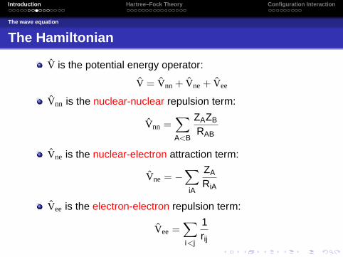
V is the potential energy operator:
V = Vnn + Vne + Vee
Vnn is the nuclear-nuclear repulsion term:
Vnn =∑A<B
ZAZB
RAB
Vne is the nuclear-electron attraction term:
Vne = −∑iA
ZA
RiA
Vee is the electron-electron repulsion term:
Vee =∑i<j
1rij

Introduction Hartree–Fock Theory Configuration Interaction
The wave equation
Atomic units
All quantum chemical calculations use a special system of unitswhich, while not part of the SI, are very natural and greatlysimplify expressions for various quantities.
The length unit is the bohr (a0 = 5.29× 10⁻¹¹m)
The mass unit is the electron mass (me = 9.11× 10⁻³¹kg)
The charge unit is the electron charge (e = 1.60× 10⁻¹⁹C)
The energy unit is the hartree (Eh = 4.36× 10⁻¹⁸J)
For example, the energy of the H atom is -0.5 hartree. In morefamiliar units this is −1,313 kJ/mol

Introduction Hartree–Fock Theory Configuration Interaction
The wave equation
The hydrogen atom
We will use the nucleus as the centre of our coordinates.
The Hamiltonian is then given by:
H = Tn + Te + Vnn + Vne + Vee
= −12∇2
r −1r
And the wavefunction is simply a function of r: Ψ(r)

Introduction Hartree–Fock Theory Configuration Interaction
The wave equation
The Born-Oppenheimer approximation
Nuclei are much heavier than electrons (the mass of aproton ≈ 2000 times that of an electron) and thereforetravel much more slowly.
We assume the electrons can react instantaneously to anymotion of the nuclei (think of a fly around a rhinoceros).
This assumption allows us to factorise the wave equation:
Ψ(R, r) = Ψn(R)Ψe(r; R)
where the ‘;’ notation indicates a parametric dependence.
The potential energy surface is a direct consequence ofthe BO approximation.

Introduction Hartree–Fock Theory Configuration Interaction
Computing chemistry
The chemical connection
So far we have focused mainly on obtaining the totalenergy of our system.
Many chemical properties can be obtained from derivativesof the energy with respect to some external parameterExamples of external parameters include:
Geometric parameters (bond lengths, angles etc.)External electric field (for example from a solvent or othermolecule in the system)External magnetic field (NMR experiments)
1st and 2nd derivatives are commonly available and used.
Higher derivatives are required for some properties, butare expensive (and difficult!) to compute.
Some derivatives must be computed numerically.

Introduction Hartree–Fock Theory Configuration Interaction
Computing chemistry
Computable properties
Many molecular properties can be computed, these include
Bond energies and reaction energies
Structures of ground-, excited- and transition-states
Atomic charges and electrostatic potentials
Vibrational frequencies (IR and Raman)
Transition energies and intensities for UV and IR spectra
NMR chemical shifts
Dipole moments, polarisabilities and hyperpolarisabilities
Reaction pathways and mechanisms

Introduction Hartree–Fock Theory Configuration Interaction
Computing chemistry
Statement of the problem
The SWE is a second-order linear differential equation.Exact solutions exist for only a small number of systems:
The rigid rotorThe harmonic oscillatorA particle in a boxThe hydrogenic ions (H, He+, Li2+ . . .)
Approximations must be used:Hartree-Fock theory a wavefunction-based approach thatrelies on the mean-field approximation.Density Functional Theory whose methods obtain theenergy from the electron density rather than the (morecomplicated) wavefunction.
Relativity is usually ignored.

Introduction Hartree–Fock Theory Configuration Interaction
Computing chemistry
Classification of methods
Post-HF
DFT HF
ΨEc
SCF
Hybrid DFT

Introduction Hartree–Fock Theory Configuration Interaction
Lecture
1 IntroductionBackgroundThe wave equationComputing chemistry
2 Hartree–Fock TheoryThe molecular orbital approximationThe self-consistent fieldRestricted and unrestricted HF theory
3 Configuration InteractionThe correlation energyConfiguration expansion of the wavefunction
Introduction Hartree–Fock Theory Configuration Interaction
Previously on 3108
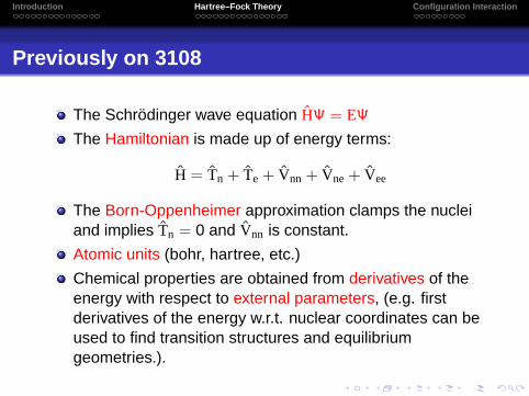
The Schrodinger wave equation HΨ = EΨ
The Hamiltonian is made up of energy terms:
H = Tn + Te + Vnn + Vne + Vee
The Born-Oppenheimer approximation clamps the nucleiand implies Tn = 0 and Vnn is constant.
Atomic units (bohr, hartree, etc.)
Chemical properties are obtained from derivatives of theenergy with respect to external parameters, (e.g. firstderivatives of the energy w.r.t. nuclear coordinates can beused to find transition structures and equilibriumgeometries.).

Introduction Hartree–Fock Theory Configuration Interaction
Classification of methods
Post-HF
DFT HF
ΨEc
SCF
Hybrid DFT

Introduction Hartree–Fock Theory Configuration Interaction
The molecular orbital approximation
Hartree-Fock theory
HF theory is the simplest wavefunction-based method.
It forms the foundation for more elaborate electronicstructure methods.
It is synonymous with the Molecular Orbital Approximation.It relies on the following approximations:
The Born-Oppenheimer approximationThe independent electron approximationThe linear combination of atomic orbitals approximation
It does not model the correlation energy, by definition.

Introduction Hartree–Fock Theory Configuration Interaction
The molecular orbital approximation
Hartree-Fock theory
Consider the H2 molecule:
The total wavefunction involves 4 coordinates:Ψ = Ψ(R1,R2, r1, r2)
We invoke the Born-Oppenheimer approximation:Ψ = Ψn(R1,R2)Ψe(r1, r2).
How do we model Ψe(r1, r2)?

Introduction Hartree–Fock Theory Configuration Interaction
The molecular orbital approximation
The Hartree wavefunction
We assume the wavefunction can be written as a Hartreeproduct: Ψ(r1, r2) = ψ1(r1)ψ2(r2)
The individual one-electron wavefunctions, ψi are calledmolecular orbitals.
This form of the wavefunction does not allow forinstantaneous interactions of the electrons.
Instead, the electrons feel the averaged field of all theother electrons in the system.
The Hartree form of the wavefunction is is sometimescalled the independent electron approximation.

Introduction Hartree–Fock Theory Configuration Interaction
The molecular orbital approximation
The Pauli principle
One of the postulates of quantum mechanics is that thetotal wavefunction must be antisymmetric with respect tothe interchange of electron coordinates
The Pauli Principle is a consequence of antisymmetry.
The Hartree wavefunction is not antisymmetric:
Ψ(r2, r1) = ψ1(r2)ψ2(r1) 6= −Ψ(r1, r2)
We can make the wavefunction antisymmetric by adding allsigned permutations:
Ψ(r1, r2) =1√2
[ψ1(r1)ψ2(r2)− ψ1(r2)ψ2(r1)
]

Introduction Hartree–Fock Theory Configuration Interaction
The molecular orbital approximation
The Hartree-Fock wavefunction
The antisymmetrized wavefunction is called theHartree-Fock wavefunction.
It can be written as a Slater determinant:
Ψ =1√N!
∣∣∣∣∣∣∣∣∣ψ1(r1) ψ2(r1) · · · ψN(r1)ψ1(r2) ψ2(r2) · · · ψN(r2)
......
. . ....
ψ1(rN) ψ2(rN) · · · ψN(rN)
∣∣∣∣∣∣∣∣∣This ensures the electrons are indistinguishable and aretherefore associated with every orbital!
A Slater determinant is often written as |ψ1, ψ2, . . . ψN〉

Introduction Hartree–Fock Theory Configuration Interaction
The molecular orbital approximation
The LCAO approximation
The HF wavefunction is an antisymmetric wavefunctionwritten in terms of the one-electron MOs.
What do the MOs look like?
We write them as a linear combination of atomic orbitals:
ψi(r i) =∑
µ
Cµiχµ(r i)
The χµ are atomic orbitals or basis functions.
The Cµi are MO coefficients.

Introduction Hartree–Fock Theory Configuration Interaction
The molecular orbital approximation
An example
The H2 molecule:
ψ1 = σ = 1√2
(χA
1s + χB1s
)ψ2 = σ∗ = 1√
2
(χA
1s − χB1s
)
For H2 the MO coefficients, Cµi , are ± 1√2

Introduction Hartree–Fock Theory Configuration Interaction
The molecular orbital approximation
The HF energy
If the wavefunction is normalized, the expectation value ofthe energy is given by: E = 〈Ψ|H|Ψ〉For the HF wavefunction, this can be written:
EHF =∑
i
Hi +12
∑ij
(Jij − Kij)
Hi involves one-electron terms arising from the kineticenergy of the electrons and the nuclear attraction energy.
Jij involves two-electron terms associated with the coulombrepulsion between the electrons.
Kij involves two-electron terms associated with theexchange of electronic coordinates.

Introduction Hartree–Fock Theory Configuration Interaction
The molecular orbital approximation
The HF energy
Remember that our wavefunction is given in terms of adeterminant: |ψ1, ψ2, . . . ψN〉And our MOs are written as a LCAO:
ψi(r i) =∑
µ
Cµiχµ(r i)
We can write the one-electron parts of the energy as:
Hi = 〈ψi |h|ψi〉=
∑µν
CµiCνi〈χµ|h|χν〉
The Jij and Kij matrices can also be written in terms of theMO coefficients, Cµi .

Introduction Hartree–Fock Theory Configuration Interaction
The self-consistent field
The variational principle
The MO coefficients, Cµi , can be determined using thevariational theorem.
Variational TheoremThe energy determined from any approximate wavefunction willalways be greater than the energy for the exact wavefunction.
The energy of the exact wavefunction serves as a lowerbound on the calculated energy and therefore the Cµi canbe simply adjusted until the total energy of the system isminimised.

Introduction Hartree–Fock Theory Configuration Interaction
The self-consistent field
The self-consistent field method
Thus, computing the HF energy implies computing the Cµi .
To compute the Cµi we must minimise the HF energyaccording to the variational principle.
Which comes first: the HF energy or the Cµi?
The SCF Process1 Guess a set of MOs, Cµi
2 Use MOs to compute Hi , Jij and Kij
3 Solve the HF equations for the energy and new MOs4 Are the new MOs different? Yes → (2) : No → (5)5 Self-consistent field converged

Introduction Hartree–Fock Theory Configuration Interaction
Restricted and unrestricted HF theory
Electron Spin
So far for simplicity we have ignored the spin variable, ω.
Each MO actually contains a spatial part and a spin part.
For each spatial orbital, there are two spin orbitals:χα
i (r, ω) = φi(r)α(ω) and χβi (r, ω) = φi(r)β(ω).
This is reasonable for closed-shell systems, but not foropen-shell systems.
H2 H−2

Introduction Hartree–Fock Theory Configuration Interaction
Restricted and unrestricted HF theory
Restricted and unrestricted HF theory
The spatial part of the spinorbitals are the same:
φαi = φβ
i
The spatial part of the spinorbitals are different:
φαi 6= φβ
i

Introduction Hartree–Fock Theory Configuration Interaction
Restricted and unrestricted HF theory
Pros and cons
Advantages of the Unrestricted Hartree-Fock method:
Accounts for spin-polarisation, the process by whichunpaired electrons perturb paired electrons, and thereforegives realistic spin densities.
Provides a qualitatively correct description ofbond-breaking.
Provides a better model for systems with unpairedelectrons.
Disadvantages of the UHF method:
Calculations take slightly longer to perform than for RHF.
Can lead to spin-contamination which means thewavefunction is no longer a spin-eigenfunction (as it shouldbe).

Introduction Hartree–Fock Theory Configuration Interaction
Restricted and unrestricted HF theory
Previously on 3108
The MO approximation and the Hartree wavefunction:
Ψ(r1, r2) = ψ1(r1)ψ2(r2)
Antisymmetry and the Hartree-Fock wavefunction:
Ψ(r1, r2) =1√2
[ψ1(r1)ψ2(r2)− ψ1(r2)ψ2(r1)
]The LCAO approximation
ψi(r i) =∑
µ
Cµiχµ(r i)
The variational method and self-consistent field calculation
Restricted and unrestricted Hartree-Fock theory

Introduction Hartree–Fock Theory Configuration Interaction
Restricted and unrestricted HF theory
Classification of methods
Post-HF
DFT HF
ΨEc
SCF
Hybrid DFT

Introduction Hartree–Fock Theory Configuration Interaction
Lecture
1 IntroductionBackgroundThe wave equationComputing chemistry
2 Hartree–Fock TheoryThe molecular orbital approximationThe self-consistent fieldRestricted and unrestricted HF theory
3 Configuration InteractionThe correlation energyConfiguration expansion of the wavefunction

Introduction Hartree–Fock Theory Configuration Interaction
The correlation energy
Energy decomposition
The electronic Hamiltonian (energy operator) has severalterms:
Hel = Te(r) + Vne(r; R) + Vee(r)
This operator is linear, thus the electronic energy can alsobe written as a sum of several terms:
Eel = ET + EV︸ ︷︷ ︸ + EJ + EK + EC︸ ︷︷ ︸Te + Vne Vee
Where we have broken down the electron-electronrepulsion energy into three terms: EJ + EK + EC

Introduction Hartree–Fock Theory Configuration Interaction
The correlation energy
Electronic energy decomposition
EJ is the coulomb repulsion energyThis energy arises from the classical electrostatic repulsionbetween the charge clouds of the electrons and is correctlyaccounted for in the Hartree wavefunction.
EK is the exchange energyThis energy directly arises from making the wavefunctionantisymmetric with respect to the interchange of electroniccoordinates, and is correctly accounted for in theHartree-Fock wavefunction.
EC is the correlation energyThis is the error associated with the mean-fieldapproximation which neglects the instantaneousinteractions of the electrons. So far we do not havewavefunction which models this part of the energy.

Introduction Hartree–Fock Theory Configuration Interaction
The correlation energy
Electronic energy decomposition
E = ET + EV + EJ + EK + EC
For the Ne atom, the above energy terms are:
ET = +129 Eh
EV = -312 Eh
EJ = +66 Eh
EK = -12 Eh 9.3%EC = -0.4 Eh 0.3%
The HF energy accounts for more than 99% of the energy
If the correlation energy is so small, can we neglect it?

Introduction Hartree–Fock Theory Configuration Interaction
The correlation energy
The importance of EC
Consider the atomisation energy of the water molecule:
Energy H2O 2 H + O ∆EEHF -76.057770 -75.811376 0.246393ECCSD -76.337522 -75.981555 0.355967
If we neglect the correlation energy in the atomisation of waterwe make a 30% error!

Introduction Hartree–Fock Theory Configuration Interaction
The correlation energy
The electron correlation energy
The correlation energy is sensitive to changes in thenumber of electron pairs
The correlation energy is always negativeThere are two components to the correlation energy:
Dynamic correlation is the energy associated with thedance of the electrons as they try to avoid one another.This is important in bond breaking processes.Static correlation arises from deficiencies in the singledeterminant wavefunction and is important in systems withstretched bonds and low-lying excited states.
Electron correlation gives rise to the inter-electronic cusp
Computing the correlation energy is the single mostimportant problem in quantum chemistry

Introduction Hartree–Fock Theory Configuration Interaction
The correlation energy
Modelling the correlation energy
There exists a plethora of methods to compute the correlationenergy, each with their own strengths and weaknesses:
Configuration interaction (CISD, CISD(T))
Møller-Plesset perturbation theory (MP2, MP3. . .)
Quadratic configuration interaction (QCISD)
Coupled-cluster theory (CCD, CCSD, CCSDT)
Multi-configuration self-consistent field theory (MCSCF)
Density functional theory (DFT)
In practice, none of these methods are exact, but they all(except for DFT) provide a well-defined route to exactitude.

Introduction Hartree–Fock Theory Configuration Interaction
Configuration expansion of the wavefunction
Configuration interaction
Recall the HF wavefunction is a single determinant madeup of the product of occupied molecular orbitals ψi :
Ψ0 = |ψ1, ψ2, . . . ψN〉
ψi =∑
µ
Cµiχµ
This is referred to as a single configuration treatment
If we have M atomic orbitals, the HF method gives us Mmolecular orbitals, but only the lowest N are occupied.
The remaining M − N orbitals are called virtual orbitals

Introduction Hartree–Fock Theory Configuration Interaction
Configuration expansion of the wavefunction
Configuration interaction
We can create different configurations by “exciting” one ormore electrons from occupied to virtual orbitals:
Ψ0 = |ψ1, ψ2, . . . ψiψj . . . ψN〉Ψa
i = |ψ1, ψ2, . . . ψaψj . . . ψN〉Ψab
ij = |ψ1, ψ2, . . . ψaψb . . . ψN〉
These configurations can be mixed together to obtain abetter approximation to the wavefunction:
ΨCI = c0Ψ0 +∑
i
cai Ψa
i +∑
ij
cabij Ψab
ij + . . .
The CI coefficients, cai , c
abij . . . can be found via the
variational method

Introduction Hartree–Fock Theory Configuration Interaction
Configuration expansion of the wavefunction
How does this help?
Consider a minimal H2 system with two MOs:
ψ1 = σ =1√2
(χA
1s + χB1s
)
ψ2 = σ∗ =1√2
(χA
1s − χB1s
)
The anti-bonding orbital, σ∗, has a node at the origin. Byallowing this orbital to mix in the electrons can spend more timeapart on average, thus lowering the repulsion energy.

Correlated Methods Basis Sets Density Functional Theory
Lecture
4 Correlated MethodsConfiguration interactionCoupled-cluster theoryPerturbation theoryComputational Cost
5 Basis SetsBasis functionsAdditional types of functions
6 Density Functional TheoryDensity functionalsThe Hohenberg–Kohn theoremsDFT models

Correlated Methods Basis Sets Density Functional Theory
Previously on 3108
The MO approximation and the Hartree wavefunction:
Ψ(r1, r2) = ψ1(r1)ψ2(r2)
Antisymmetry and the Hartree-Fock wavefunction:
Ψ(r1, r2) =1√2
[ψ1(r1)ψ2(r2)− ψ1(r2)ψ2(r1)
]The LCAO approximation
ψi(r i) =∑
µ
Cµiχµ(r i)
The variational method and self-consistent field calculation
Restricted and unrestricted Hartree-Fock theory

Correlated Methods Basis Sets Density Functional Theory
Previously on 3108
The origins of the electronic correlation energy
The importance of the electronic correlation energy
The idea of a configuration (determinant):
Ψ0 = |ψ1, ψ2, . . . ψiψj . . . ψN〉Ψa
i = |ψ1, ψ2, . . . ψaψj . . . ψN〉Ψab
ij = |ψ1, ψ2, . . . ψaψb . . . ψN〉
The configuration interaction wavefunction
ΨCI = c0Ψ0 +occ∑i
vir∑a
cai Ψa
i +occ∑ij
vir∑ab
cabij Ψab
ij + . . .

Correlated Methods Basis Sets Density Functional Theory
Orbital densities
!4 !2 2 4
0.1
0.2
0.3
0.4
0.5
0.6

Correlated Methods Basis Sets Density Functional Theory
Classification of methods
Post-HF
DFT HF
ΨEc
SCF
Hybrid DFT

Correlated Methods Basis Sets Density Functional Theory
Configuration interaction
Configuration interaction
If we allow all possible configurations to mix in then weobtain the Full-CI wavefunction. This is the most completetreatment possible for a given set of basis functions.
Complete-CI is Full-CI in an infinite basis set and yields theecact non-relativistic energy.
The cost of full-CI scales exponentially and is thereforeonly feasible for molecules with around 12 electrons andmodest basis sets.Truncated CI methods limit the types of excitations that canoccur:
CIS adds only single excitations (same as HF!)CID adds only double excitationsCISD adds single and double excitationsCISDT adds single, double and triple excitations
Correlated Methods Basis Sets Density Functional Theory
Configuration interaction
Size consistency
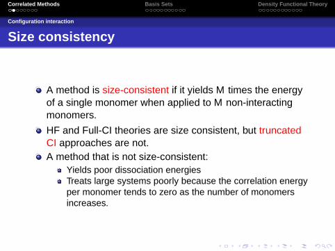
A method is size-consistent if it yields M times the energyof a single monomer when applied to M non-interactingmonomers.
HF and Full-CI theories are size consistent, but truncatedCI approaches are not.A method that is not size-consistent:
Yields poor dissociation energiesTreats large systems poorly because the correlation energyper monomer tends to zero as the number of monomersincreases.

Correlated Methods Basis Sets Density Functional Theory
Coupled-cluster theory
Coupled-cluster theories
The CID wavefunction can be written as ΨCID = (1 + T2)Ψ0
where:
T2 =14
occ∑i
occ∑j
virt∑a
virt∑b
cabij aaaba∗i a∗j
The a and a∗ are creation and annihilation operators.
The CCD wavefunction can then be written as :
ΨCCD = exp (T2)Ψ0
=
[1 + T2 +
T 22
2!+
T 32
3!+ . . .
]Ψ0
T 22 gives some quadruple excitations and leads to
size-consistency

Correlated Methods Basis Sets Density Functional Theory
Perturbation theory
The HF Hamiltonian
The Hartree-Fock wavefunction is not an eigenfunction ofthe Hamiltonian HΨ0 6= EHFΨ0
However, it can be considered as an eigenfunction of theHartree–Fock Hamiltonian:
H0 =∑
i
f (r i)
f (r i) = T(r i) + Vne(r i) + νHF(r i)
The difference between these operators, H− H0 gives thecorrelation energy
Correlated Methods Basis Sets Density Functional Theory
Perturbation theory
Møller-Plesset perturbation theory
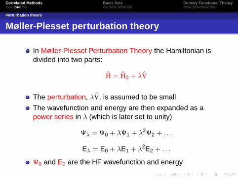
In Møller-Plesset Perturbation Theory the Hamiltonian isdivided into two parts:
H = H0 + λV
The perturbation, λV, is assumed to be small
The wavefunction and energy are then expanded as apower series in λ (which is later set to unity)
Ψλ = Ψ0 + λΨ1 + λ2Ψ2 + . . .
Eλ = E0 + λE1 + λ2E2 + . . .
Ψ0 and E0 are the HF wavefunction and energy

Correlated Methods Basis Sets Density Functional Theory
Perturbation theory
Møller-Plesset perturbation theory
MPn is obtained by truncating the expansion at order λn
The MP1 energy is the same as the HF energy
The MP2 energy is given by:
EMP2 =occ∑i<j
vir∑a<b
|〈Ψ0|V|Ψabij 〉|
2
εi + εj − εa − εb
The cost of calculating the MP2 energy scales as O(N5)and typically recovers ∼80-90% of the correlation energy
The MPn energy is size-consistent but not variational
The MP series may diverge for large orders

Correlated Methods Basis Sets Density Functional Theory
Computational Cost
Scaling
HF formally scales asO(N4), practically as O(N2)
MPn scales as O(Nn+3)
CCSD and CISD scale asO(N6)
CCSD(T) scales as O(N7)
CCSDT scales as O(N8)

Correlated Methods Basis Sets Density Functional Theory
Computational Cost
An example
System tHF tMP2 tCCSD
Ala1 2.6 s 40 s 58 mAla2 47 s 6 m 30 sAla3 3m 20 s 30 m 50 sAla4 8m 20 s

Correlated Methods Basis Sets Density Functional Theory
Lecture
4 Correlated MethodsConfiguration interactionCoupled-cluster theoryPerturbation theoryComputational Cost
5 Basis SetsBasis functionsAdditional types of functions
6 Density Functional TheoryDensity functionalsThe Hohenberg–Kohn theoremsDFT models

Correlated Methods Basis Sets Density Functional Theory
Previously on 3108
Correlated wavefunction methods:
Theory Ψ Variational Size-ConsistentCI (1 + T1 + T2 + . . .)Ψ0 ✓ ✗
CC exp(T1 + T2 + . . .)Ψ0 ✗ ✓
MP Ψ0 + λΨ1 + λ2Ψ2 + . . . ✗ ✓
Each of these methods gives a hierarchy to exactitude
Full-CI gives the exact energy (within the given basis set)
The concepts of variational and size-consistent methods
Coupled-cluster methods are currently the most accurategenerally applicable methods in quantum chemistry
CCSD(T) has been called the “gold standard” and iscapable of yielding chemical accuracy

Correlated Methods Basis Sets Density Functional Theory
Basis functions
Basis functions
The atom-centred functions used to describe the atomicorbitals are known as basis functions and collectively forma basis set
Larger basis sets give a better approximation to the atomicorbitals as the place fewer restrictions on the wavefunction
Larger basis sets attract a higher computational cost
Basis sets are carefully designed to give the bestdescription for the lowest cost

Correlated Methods Basis Sets Density Functional Theory
Basis functions
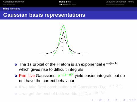
Gaussian basis representations
The 1s orbital of the H atom is an exponential e−α|r−A|
which gives rise to difficult integrals
Primitive Gaussians, e−β|r−A|2 yield easier integrals but donot have the correct behaviour
If we take fixed combinations of Gaussians {Die−βi |r−A|2}...we get the best of both worlds
∑i Die−βi |r−A|2
Correlated Methods Basis Sets Density Functional Theory
Basis functions
Gaussian basis representations
The 1s orbital of the H atom is an exponential e−α|r−A|
which gives rise to difficult integrals
Primitive Gaussians, e−β|r−A|2 yield easier integrals but donot have the correct behaviour
If we take fixed combinations of Gaussians {Die−βi |r−A|2}...we get the best of both worlds
∑i Die−βi |r−A|2

Correlated Methods Basis Sets Density Functional Theory
Basis functions
Gaussian basis functions
A Cartesian Gaussian basis function can be written:
χ(x , y , z) = xaybzcK∑
i=1
Die−αi (x2+y2+z2)
a + b + c is the angular momentum of χ
K is the degree of contraction of χ
Di are the contraction coefficients of χ
αi are the exponents of χ
These types of basis functions are sometimes referred toas GTOs

Correlated Methods Basis Sets Density Functional Theory
Basis functions
Minimal basis sets
The simplest possible atomic orbital representation iscalled a minimal basis set
Minimal basis sets contain the minimum number of basisfunctions to accommodate all of the electrons in the atom
For example:H & He a single function (1s)1st row 5 functions, (1s,2s,2px ,2py ,2pz)2nd row 9 functions, (1s,2s,2px ,2py ,2pz ,3s,3px ,3py ,3pz)
Functions are always added in shells

Correlated Methods Basis Sets Density Functional Theory
Basis functions
Minimal basis sets
The STO-3G basis set is a minimal basis set where eachatomic orbital is made up of 3 Gaussians. STO-nG alsoexist.
Minimal basis sets are not well suited to model theanisotropic effects of bonding
Because the exponents do not vary, the orbitals have afixed size and therefore cannot expand or contract

Correlated Methods Basis Sets Density Functional Theory
Additional types of functions
Split valence functions
Split-valence basis sets model each valence orbital by twoor more basis functions that have different exponents
They allow for size variations that occur in bonding
Examples include the double split valence basis sets,3-21G and 6-31G, and triple split valence basis sets suchas 6-311G

Correlated Methods Basis Sets Density Functional Theory
Additional types of functions
Polarisation functions
Polarisation functions have higher angular momentum
They allow for anisotropic variations that occur in bondingand help model the inter-electronic cusp
Examples include 6-31G(d) or 6-31G* which include dfunctions on the heavy atoms 6-31G(d ,p) or 6-31G**which include d functions on heavy atoms and p functionson hydrogen atoms

Correlated Methods Basis Sets Density Functional Theory
Additional types of functions
Diffuse functions
Diffuse basis functions are additional functions with smallexponents, and are therefore largeThey allow for accurate modelling of systems with weaklybound electrons, such as
AnionsExcited states
A set of diffuse functions usually includes a diffuse s orbitaland a set of diffuse p orbitals with the same exponent
Examples in include 6-31+G which has diffuse functions onthe heavy atoms and 6-31++G which has diffuse functionson hydrogen atoms as well.

Correlated Methods Basis Sets Density Functional Theory
Additional types of functions
Mix and match
Larger basis sets can be built up from these components,for example 6-311++G(2df ,2dp)
Dunning basis sets also exist, for example pVDZ and pVTZFor larger atoms Effective Core Potentials (ECPs) are oftenused. These replace the core electrons with an effectivepotential and have two main advantages:
They reduce the number of electrons (cheaper)They can be parameterized to take account of relativity
The valence electrons are still modelled using GTOs

Correlated Methods Basis Sets Density Functional Theory
Additional types of functions
Examples
Basis set Description No. functionsH C,O H2O C6H6
STO-3G Minimal 1 5 7 363-21G Double split-valence 2 9 13 66
6-31G(d) Double split-valence with polari-
sation
2 15 19 102
6-31G(d ,p) Ditto, with p functions on H 5 15 25 1206-311+G(d ,p) Triple split-valence with polarisa-
tion, p functions on H and diffuse
functions on heavy atoms
6 22 34 168

Correlated Methods Basis Sets Density Functional Theory
Additional types of functions
Accuracy
The accuracy of the computed properties is sensitive to thequality of the basis set. Consider the bond length anddissociation energy of the hydrogen fluoride molecule:
Basis set Bond Length (A) D0 (kJ/mol)6-31G(d) 0.9337 4916-31G(d ,p) 0.9213 5236-31+G(d) 0.9408 5156-311G(d) 0.9175 4846-311+G(d ,p) 0.9166 551Expt. 0.917 566
ZPVE = 25 kJ/mol MP2/6-311+G(d ,p)

Correlated Methods Basis Sets Density Functional Theory
Lecture
4 Correlated MethodsConfiguration interactionCoupled-cluster theoryPerturbation theoryComputational Cost
5 Basis SetsBasis functionsAdditional types of functions
6 Density Functional TheoryDensity functionalsThe Hohenberg–Kohn theoremsDFT models

Correlated Methods Basis Sets Density Functional Theory
Previously on 3108
Gaussian basis functionsPrimitive functionsContracted basis functions
Minimal basis setsAdditional types of functions
Split valencePolarisation functionsDiffuse functions
Effective Core Potentials (ECPs)

Correlated Methods Basis Sets Density Functional Theory
Classification of methods
Post-HF
DFT HF
ΨEc
SCF
Hybrid DFT

Correlated Methods Basis Sets Density Functional Theory
Density functionals
What is the density?
The electron density is a fundamental quantity in quantumchemistry
ρ(r1) =
∫· · ·
∫Ψ∗(r1, r2, . . . , rN)Ψ(r1, r2, . . . , rN)dr2 . . .drN
ρ(r)dr gives the probability of finding an electron in thevolume element dr
It is a function of three variables (x , y , z) and is therefore(relatively) easy to visualise

Correlated Methods Basis Sets Density Functional Theory
Density functionals
What is a functional?
A function takes a number and returns another number:
f (x) = x2 − 1 f (3) = 8
An operator takes a function and returns another function:
D(f ) = dfdx D(x2 − 1) = 2x
A functional takes a function and returns a number:
F [f ] =∫ 1
0 f (x)dx F [x2 − 1] = −2/3

Correlated Methods Basis Sets Density Functional Theory
Density functionals
What is a density functional?
A density functional takes the electron density and returnsa number, for example:
N[ρ] =
∫ρ(r)dr
simply gives the number of electrons in the molecule
Density functional theory (DFT) focusses on functionalsthat return the energy of the system

Correlated Methods Basis Sets Density Functional Theory
Density functionals
What is a density functional?
E = ET + EV + EJ + EK + EC
The classical potential energy terms of the total energy canbe expressed exactly in terms of the density:
EJ =12
∫ ∫ρ(r1)ρ(r2)
|r1 − r2|dr1dr2
EV = −∑
A
∫ZAρ(r)|RA − r|
dr
What about ET, EK and EC?

Correlated Methods Basis Sets Density Functional Theory
Density functionals
Orbital functionals
In Hartree-Fock theory, ET, EK and EC, are all orbitalfunctionals, eg:
ET = −12
∑i
∫ψi(r)∇2ψi(r)dr
No (known) exact expression for the kinetic energy interms of ρ exists
The exchange energy is non-classical, so should weexpect there to be an expression for the exchange energyin terms of the classical density?

Correlated Methods Basis Sets Density Functional Theory
The Hohenberg–Kohn theorems
The Hohenberg–Kohn theorems
The First Hohenberg-Kohn Theorem
The electron density ρ(r) determines the external potential
This theorem establishes the existence of a (universal andunique) energy functional of the density
The Second Hohenberg-Kohn Theorem
Any approximate density ρ which provides the external potentialν(r), determines its own wavefunction.
The second HK theorem can be used to establish avariational principle for DFT, although it restricts the theoryto ground states

Correlated Methods Basis Sets Density Functional Theory
The Hohenberg–Kohn theorems
The Hohenberg–Kohn theorems
The HK theorems are non-constructive, so we don’t knowwhat the form of the universal functional is
Research in the DFT largely falls down to the developmentof approximate functionals that model experimental data
Kinetic energy functionals are particularly problematic asET is so large and even a small relative error gives largeabsolute errors
Almost all DFT calculations rely on the Kohn-Shamapproximation, which avoids the need for a kinetic energyfunctional
Different DFT methods differ in the way they represent EX
and EC

Correlated Methods Basis Sets Density Functional Theory
DFT models
The uniform electron gas
The uniform electron gas is a model system with aconstant density of electrons
In 1930 Dirac showed that the exact exchange energy forthis system is given by:
EX = −Cx
∫ρ4/3(r)dr
Much later, Vosko, Wilk and Nusair parameterised acorrelation functional based on the UEG, its form is morecomplicated and it is inexact

Correlated Methods Basis Sets Density Functional Theory
DFT models
Local density approximation
Applying the UEG functionals to molecular system is calledthe local (spin) density approximation (LDA)
Combining the Dirac and VWN expressions gives theS-VWN functional
The LDA functional for EX underestimates the trueexchange energy by about 10% whereas the VWNfunctional overestimates EC by as much as 100%
Together they overbind molecular systems
The constant Cx is sometimes scaled to account for theover-binding, this gives Xα theory

Correlated Methods Basis Sets Density Functional Theory
DFT models
Gradient corrected functionals
Gradient corrected functions depend on ∇ρ as well as ρ
The gradient helps to account for deviations fromuniformity in molecular systems
The generalised gradient approximation exchangefunctionals have the form
EX =
∫ρ4/3(r)g(x)dr
where x is the reduced gradient
Different GGAs, such as Perdew ’86 and Becke ’88 aredefined by different g(x) functions

Correlated Methods Basis Sets Density Functional Theory
DFT models
GGA correlation functionals
There are also GGA correlation functionals such asLee-Yang-Parr (LYP) and Perdew ’86
EX and EC can be mixed and matched, although certaincombinations such as BLYP work particularly well
Combining a correlation functional with Hartree-Fockexchange does not work well, but hybrid functionals do:
EB3LYP = (1−c1)ED30X +c1EFock
K +c2EB88X +(1−c3)EVWN
C +c3ELYPC
B3LYP is the most popular density functional that is usedand yields very good structural and thermochemicalproperties

Correlated Methods Basis Sets Density Functional Theory
DFT models
Strengths and weaknesses
Advantages of DFT methods include:
Low computational cost
Good accuracy for structures and thermochemistry
The density is conceptually more simple than Ψ
Disdvantages of DFT methods include:
Can fail spectacularly and unexpectedly
No systematic way of improving the results
Integrals require numerical quadrature grids

Model Chemistries
Lecture
7 Model ChemistriesModel chemistries

Model Chemistries
Model chemistries
Levels of theory
Quantum chemistry abounds with many levels of theorythat represent a trade-off between computational cost andaccuracyA minimal basis Hartree-Fock calculation forms ourbaseline, other level of theory distinguish themselves bytheir treatment of the correlation energy and the size of thebasis
Cost favours small basis sets and a low-level treatment ofcorrelationAccuracy favours large basis sets and a high-leveltreatment of correlation

Model Chemistries
Model chemistries
The Pople Diagram
HF MP2 MP3 MP4 CCSD(T) · · · Full CI
Minimal Low-level · · · · · · · · · UnbalancedSplit-Valence . . . . . .PolarisedDiffuse . . .Polarised +Diffuse
... . . .. . .
Infinite Unbalanced Exact!

Model Chemistries
Model chemistries
Establishing the reliability of a method
Experimental data forms a valuable means of establishingthe reliability of a particular level of theory
Data sets such as the G2 and G3 sets are made up ofaccurate experimental values with uncertainties of lessthan 1 kcal/mol (chemical accuracy)
The G2 set consists of thermochemical data includingatomisation energies, ionisation potentials, electronaffinities and proton affinities for a range of smallmolecules (1 or 2 heavy atoms)
These data set can be used to benchmark a level of theory
What if we want to apply our method to an unknownsystem?

Model Chemistries
Model chemistries
Establishing the reliability of a method
If we wish to apply a level of theory to a system that has noexperimental data available, we need to converge the levelof theory to have confidence in our results
We start near the top left-hand (cheap) corner of the Poplediagram and move towards the bottom right-hand(expensive) corner carrying out several calculations
When we see no improvement in the result, then weconclude that we have the correct answer
Note that we cannot apply this approach to DFT methods(although we can converge the basis set)

Model Chemistries
Model chemistries
Specifying the level of theory
Geometric properties converge faster (with respect to thelevel of theory) than the energy (they are less sensitive tocorrelation)
It is common to optimise the geometry at a low-level oftheory, and then compute the energy at a higher level oftheory
The notation for this isenergy-method/basis-set//geometry-method/basis-set
For example:CCSD(T)/6-311G(2d,p)//HF/6-31G

Model Chemistries
Model chemistries
Performance
Average deviation from experiment for bond-lengths of 108main group molecules using 6-31G(d ,p)
Bond-length HF MP2 LDA GGA HybridDeviation A 0.021 0.014 0.016 0.017 0.011
Average deviation from experiment for atomisation energies of108 main group molecules using 6-31G(d ,p)
AE HF MP2 LDA GGA HybridDeviation kcal/mol 119.2 22.0 52.2 7.0 6.8

Model Chemistries
Model chemistries
Performance
Calculated electron affinity (eV) for Fluorine:
HF MP2 B3LYPSTO-3G -10.16 -10.16 -9.013-21G -1.98 -1.22 -0.866-31G(d) -0.39 +1.07 +1.056-311+G(2df ,p) +1.20 +3.44 +3.466-311+G(3df ,2p) +1.19 +3.54 +3.46Experiment +3.48