Introduction to Climate Data Homogenization techniques · Introduction to Climate Data...

Introduction to Climate Data Homogenization techniques

By Thomas Peterson

Using material stolen from Enric Aguilar*

CCRG Geography Unit

Universitat Rovira i Virgili de Tarragona Spain

* Who in turn stole material prepared by Lucie Vincent, Climate Research Branch, Meteorological Service of Canada Environment Canada

Objective

Detecting steps in climatological time series, even without the prior knowledge of the position in time and magnitude of the inhomogeneity

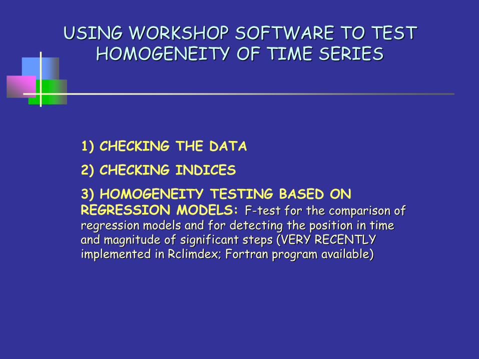
USING WORKSHOP SOFTWARE TO TEST HOMOGENEITY OF TIME SERIES

1) CHECKING THE DATA

2) CHECKING INDICES

3) HOMOGENEITY TESTING BASED ON REGRESSION MODELS: F-test for the comparison of regression models and for detecting the position in time and magnitude of significant steps (VERY RECENTLY implemented in Rclimdex; Fortran program available)

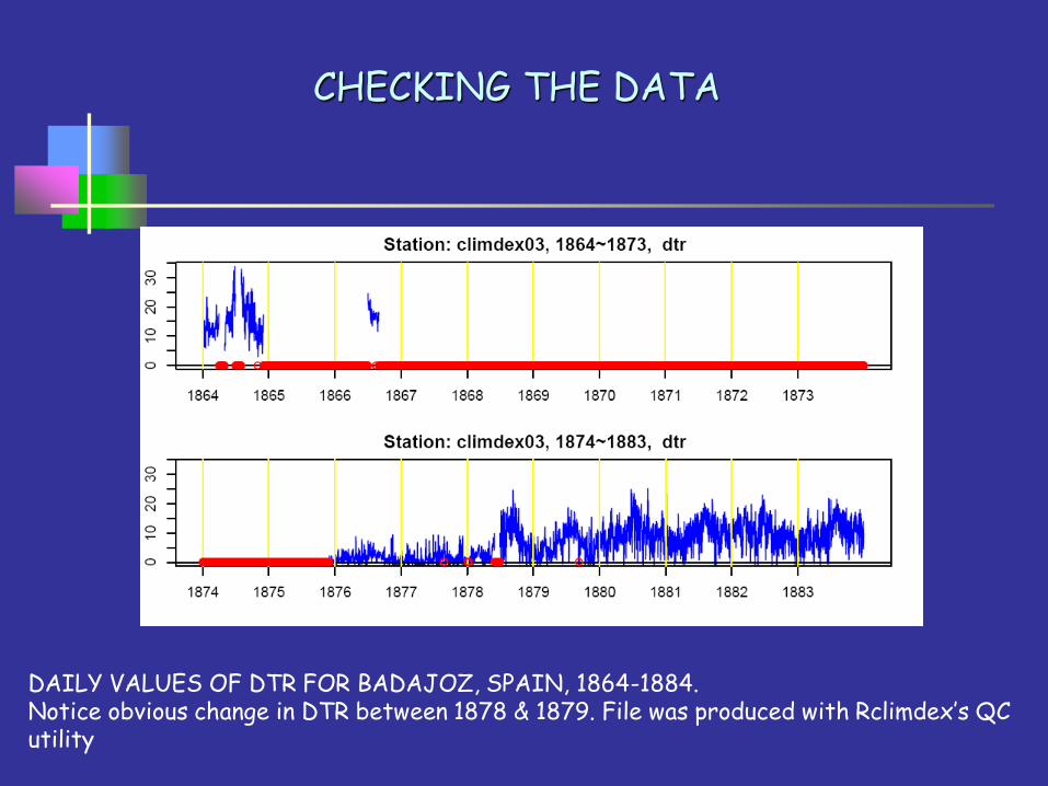
CHECKING THE DATA

DAILY VALUES OF DTR FOR BADAJOZ, SPAIN, 1864-1884. Notice obvious change in DTR between 1878 & 1879. File was produced with Rclimdex’s QC utility

CHECKING THE INDICES (I)

Data for Madrid, Spain (non-homogenized)

Obvious Change in DTR index values IN 1893.

Metadata reports a change in shelter

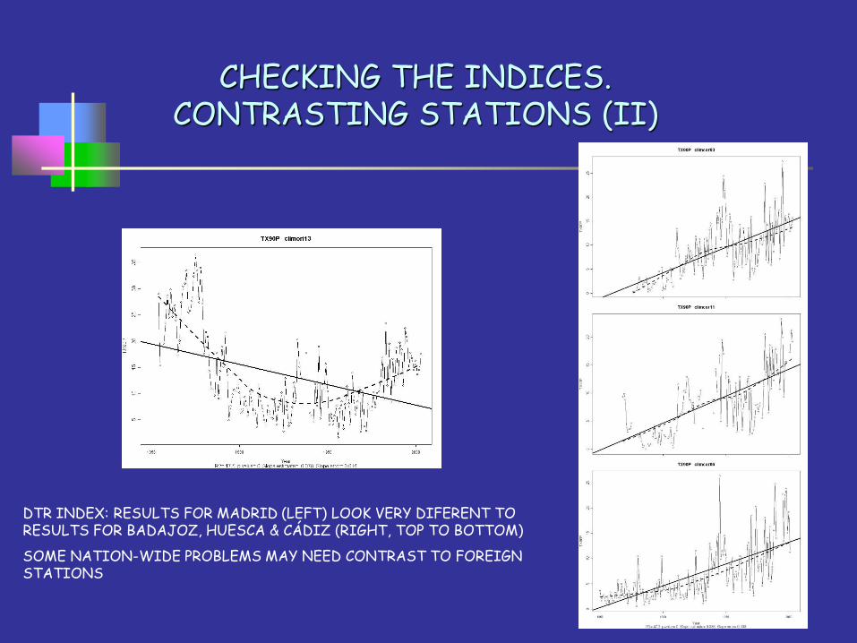
CHECKING THE INDICES. CONTRASTING STATIONS (II)

DTR INDEX: RESULTS FOR MADRID (LEFT) LOOK VERY DIFERENT TO RESULTS FOR BADAJOZ, HUESCA & CÁDIZ (RIGHT, TOP TO BOTTOM)

SOME NATION-WIDE PROBLEMS MAY NEED CONTRAST TO FOREIGN STATIONS

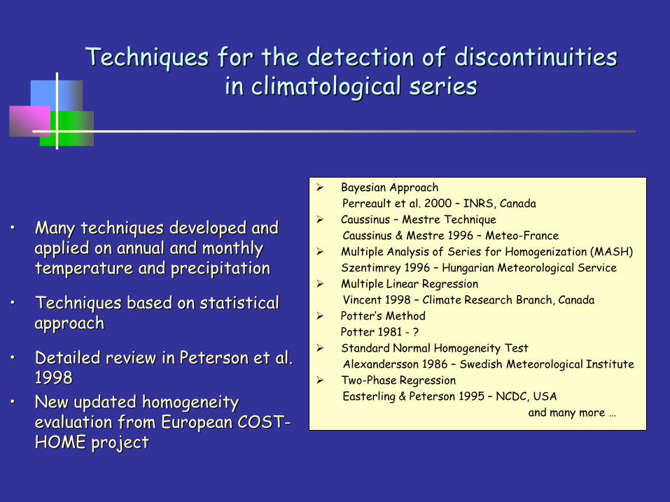
Techniques for the detection of discontinuities in climatological series

Bayesian Approach

Perreault et al. 2000 – INRS, Canada

Caussinus – Mestre Technique

Caussinus & Mestre 1996 – Meteo-France

Multiple Analysis of Series for Homogenization (MASH)

Szentimrey 1996 – Hungarian Meteorological Service

Multiple Linear Regression

Vincent 1998 – Climate Research Branch, Canada

Potter’s Method

Potter 1981 - ?

Standard Normal Homogeneity Test

Alexandersson 1986 – Swedish Meteorological Institute

Two-Phase Regression

Easterling & Peterson 1995 – NCDC, USA

and many more …

• Many techniques developed and applied on annual and monthly temperature and precipitation

• Techniques based on statistical approach

• Detailed review in Peterson et al. 1998

• New updated homogeneity evaluation from European COST-HOME project

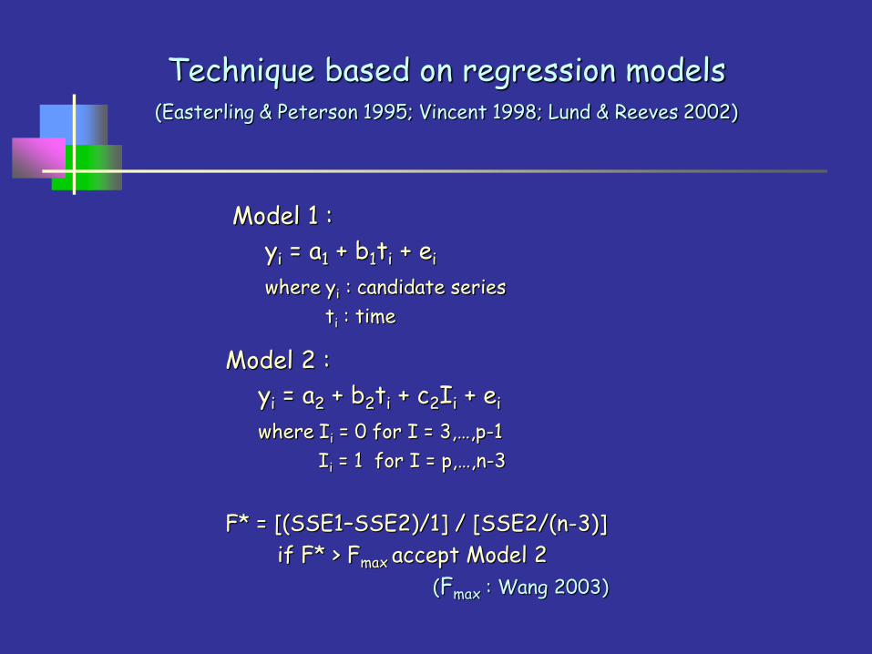
Technique based on regression models

(Easterling & Peterson 1995; Vincent 1998; Lund & Reeves 2002)

Model 2 :

yi = a2 + b2ti + c2Ii + ei

where Ii = 0 for I = 3,…,p-1

Ii = 1 for I = p,…,n-3

Model 1 :

yi = a1 + b1ti + ei

where yi : candidate series

ti : time

F* = [(SSE1–SSE2)/1] / [SSE2/(n-3)]

if F* > Fmax accept Model 2

(Fmax : Wang 2003)

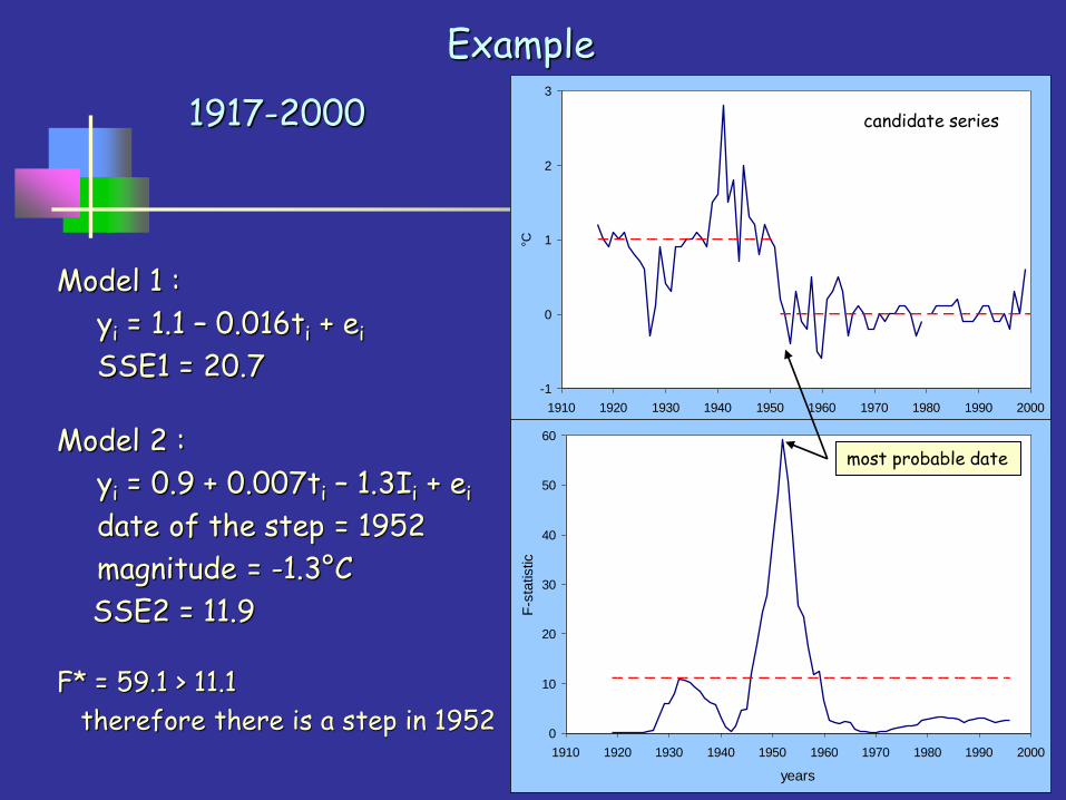
Model 2 :

yi = 0.9 + 0.007ti – 1.3Ii + ei

date of the step = 1952

magnitude = -1.3°C

SSE2 = 11.9

Model 1 :

yi = 1.1 – 0.016ti + ei

SSE1 = 20.7

F* = 59.1 > 11.1

therefore there is a step in 1952

-1

0

1

2

3

1910 1920 1930 1940 1950 1960 1970 1980 1990 2000

years

°C

candidate series

0

10

20

30

40

50

60

1910 1920 1930 1940 1950 1960 1970 1980 1990 2000

years

F-s

tatistic

1917-2000

Example

most probable date

-1

0

1

2

3

1910 1920 1930 1940 1950 1960 1970 1980 1990 2000

years

°C

Model 2 :

yi = 1.0 - 0.020ti + 0.9Ii + ei


magnitude = 0.9°C

SSE2 = 6.3

Model 1 :

yi = 0.7 + 0.019ti + ei

SSE1 = 8.6

F* = 11.3 > 11.1

therefore there is a step in 1939 0

10

20

30

40

50

60

1910 1920 1930 1940 1950 1960 1970 1980 1990 2000

years

F-s

tatistic

Example

1917-1951 candidate series

most probable date

-1

0

1

2

3

1910 1920 1930 1940 1950 1960 1970 1980 1990 2000

years

°C

Model 2 :

yi = -0.1 + 0.007ti - 0.2Ii + ei


magnitude = -0.2°C

SSE2 = 2.58

Model 1 :

yi = -0.1 + 0.002ti + ei

SSE1 = 2.59

F* = 0.01 < 11.1

therefore there is no step in 1965 0

10

20

30

40

50

60

1910 1920 1930 1940 1950 1960 1970 1980 1990 2000

years

F-s

tatistic

Example

1952-2000 candidate series

No F* > Fmax

-1

0

1

2

3

1910 1920 1930 1940 1950 1960 1970 1980 1990 2000

years

°C

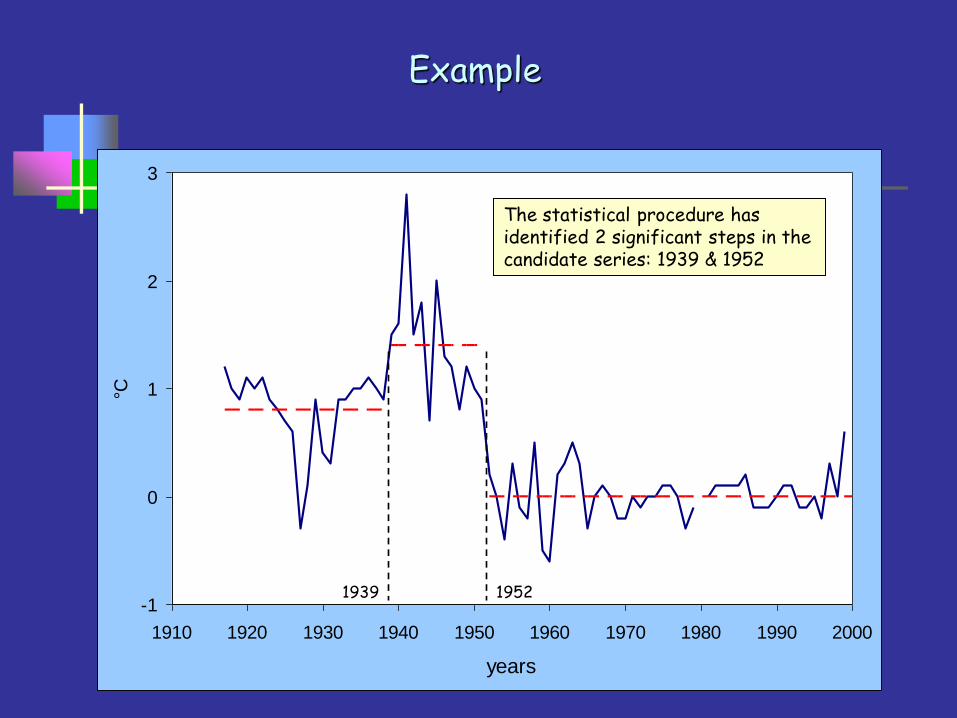
1939 1952

Example

The statistical procedure has identified 2 significant steps in the candidate series: 1939 & 1952

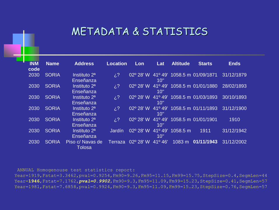
METADATA & STATISTICS

INMcode

Name Address Location Lon Lat Altitude Starts Ends

2030 SORIA Instituto 2ªEnseñanza

¿? 02º 28' W 41º 49'10''

1058.5 m 01/09/1871 31/12/1879


¿? 02º 28' W 41º 49'10''

1058.5 m 01/01/1880 28/02/1893


¿? 02º 28' W 41º 49'10''

1058.5 m 01/03/1893 30/10/1893


¿? 02º 28' W 41º 49'10''

1058.5 m 01/11/1893 31/12/1900


¿? 02º 28' W 41º 49'10''

1058.5 m 01/01/1901 1910


Jardín 02º 28' W 41º 49'10''

1058.5 m 1911 31/12/1942

2030 SORIA Piso c/ Navas deTolosa

Terraza 02º 28' W 41º 46' 1083 m 01/11/1943 31/12/2002

ANNUAL Homogenouse test statistics report:

Year=1919,Fstat=3.3462,pval=0.9254,Fm90=9.26,Fm95=11.15,Fm99=15.75,StepSize=0.4,SegmLen=44



CONCLUSIONS

- HOMOGENIZATION ASSESSMENT ON AN ANNUAL/MONTHLY BASIS WILL PREVENT MAJOR INHOMOGENEITIES TO CORRUPT THE TRENDS ANALYSIS, DISCARDING SERIES OR INHOMOGENEOUS SEGMENTS

- EVEN WHEN A CANDIDATE STATION IS/LOOKS HOMOGENEOUS AT MONTHLY & ANNUAL SCALE, INHOMOGENEITIES MAY REMAIN ON A DAILY BASIS

Thank You

Introduction to Climate Data Homogenization techniques · Introduction to Climate Data...

Documents

Transcript of Introduction to Climate Data Homogenization techniques · Introduction to Climate Data...