Introduction to Boosting

Aristotelis Tsirigosemail: tsirigos@cs.nyu.edu

SCLT seminar - NYU Computer Science

2

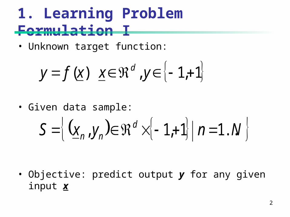
1. Learning Problem Formulation I• Unknown target function:

• Given data sample:

• Objective: predict output y for any given input x

..1 1,1, NnyxS dnn

1,1, )( yxxfy d

3

Learning Problem Formulation II• Loss function: ))(( e.g. ))(,( xhyIxhy

))(,()( xhyEhL

N

nnn xhy

NhL

1

))(,(1

)(ˆ

• Generalization error:

• Main boosting idea: minimize the empirical error:

• Objective: find h with minimum generalization error

4

PAC Learning• Input:

– Hypothesis space H– Sample of size N– Accuracy ε– Confidence 1-δ

• Objective:– Strong PAC learning: for any given ε,δ:

– Weak PAC Learning: holds only for some ε,δ

• Boosting converts a weak learner to a strong one!

)()ˆ(Pr *hLhL N

5

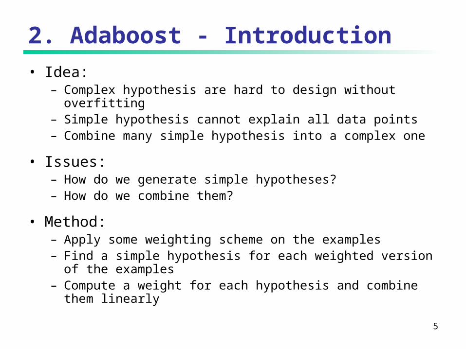
2. Adaboost - Introduction• Idea:

– Complex hypothesis are hard to design without overfitting– Simple hypothesis cannot explain all data points– Combine many simple hypothesis into a complex one

• Issues:– How do we generate simple hypotheses?– How do we combine them?

• Method:– Apply some weighting scheme on the examples– Find a simple hypothesis for each weighted version of the

examples – Compute a weight for each hypothesis and combine them

linearly

6

Some early algorithms

• Boosting by filtering (Schapire 1990)– Run weak learner on differently filtered example sets– Combine weak hypotheses– Requires knowledge on the performance of weak learner

• Boosting by majority (Freund 1995)– Run weak learner on weighted example set– Combine weak hypotheses linearly– Requires knowledge on the performance of weak learner

• Bagging (Breiman 1996)– Run weak learner on bootstrap replicates of the training set– Average weak hypotheses– Reduces variance

7

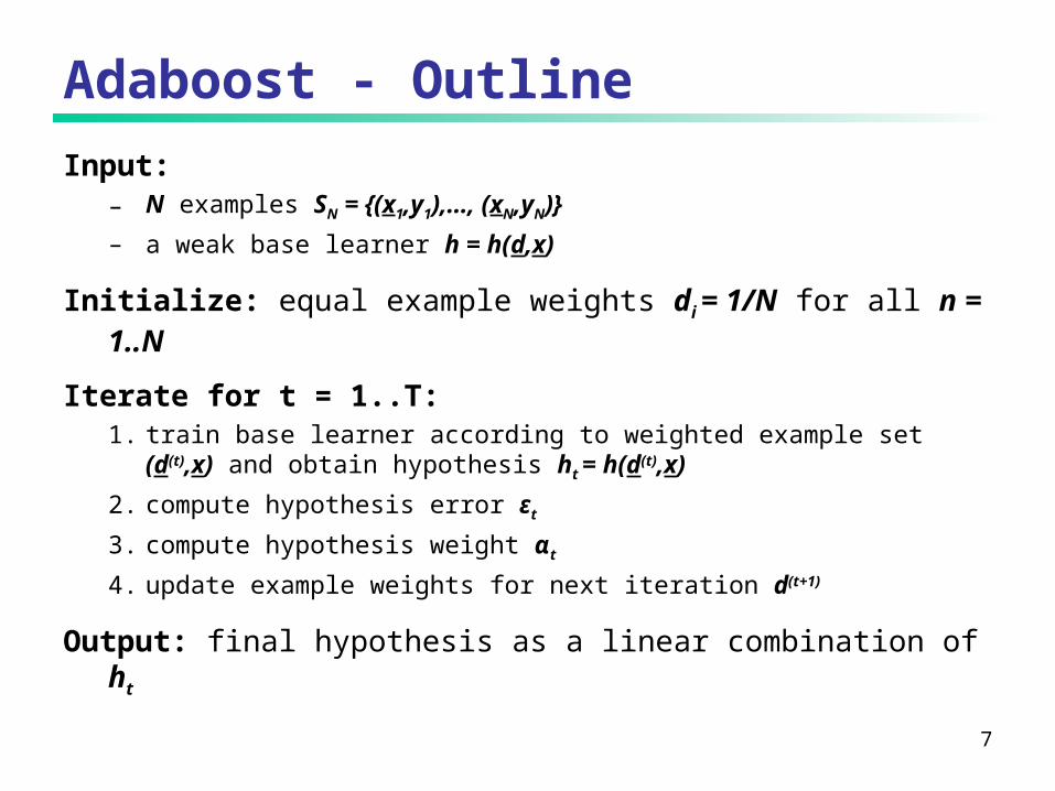
Adaboost - Outline

Input: – N examples SN = {(x1,y1),…, (xN,yN)}

– a weak base learner h = h(d,x)

Initialize: equal example weights di = 1/N for all n = 1..N

Iterate for t = 1..T:1. train base learner according to weighted example set (d(t),x)

and obtain hypothesis ht = h(d(t),x)

2. compute hypothesis error εt

3. compute hypothesis weight αt

4. update example weights for next iteration d(t+1)

Output: final hypothesis as a linear combination of ht

8

Adaboost – Data flow diagram

A(d,S) d(1)

A(d,S) d(2)

A(d,S) d(T)

SN

…

α1h1(x)

α2h2(x)αThT(x)

T

ttT

r r

tT xhxf

11

)()(

17

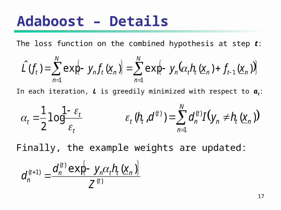
Adaboost – Details

N

nntn

tn

ttt xhyIddh

1

)()( )(),(t

tt

1log

2

1

)(

)()1( )(exp

tnttn

tnt

n Z

xhydd

The loss function on the combined hypothesis at step t:

N

nntnttn

N

nntnt xfxhyxfyfL

11

1

)()(exp)(exp)(ˆ

In each iteration, L is greedily minimized with respect to αt:

Finally, the example weights are updated:

18

Adaboost – Big picture

The weak learner A induces a feature space:

),()(: NSdAxhdhH

Ideally, we want to find the combined hypothesis with the

minimum loss:

Hh hh(x)αL argmin*

However, Adaboost optimizes α locally.

19

Base learners

• Weak learners used in practice:– Decision stumps (axis parallel splits)– Decision trees (e.g. C4.5 by Quinlan 1996)– Multi-layer neural networks– Radial basis function networks

• Can base learners operate on weighted examples?– In many cases they can be modified to accept weights along

with the examples– In general, we can sample the examples (with replacement)

according to the distribution defined by the weights

20

3. Boosting & Learning Theory

Main results

• Training error converges to zero

• Bound for the generalization error

• Bound for the margin-based generalization error

21

Training error - Definitions

Function φθ on margin z:

Empirical margin-based error:

z

zz

z

z

if,0

0 if,1

0 if,1

)( 21

N

nnnT xfy

NfL

1

))((1

)(ˆ

θ

1

10-1 z

22

Training error - Theorem

Theorem 1

The empirical margin error of the composite hypothesis fT

obeys:

T

tttTfL

1

11 )1(4)(ˆ

Therefore, the empirical margin error converges to zero

exponentially fast (for large θ).

23

Generalization bounds

Theorem 2

Let F be a class of {-1,+1}-valued functions. By applying

standard VC dimension bounds, we get that for every f in F

with probability at least 1-δ:

N

FVCcxfyPxfyP

)log()())((ˆ))((

1

This is a distribution-free bound, i.e. it holds for any

probability measure P.

24

Luckiness

• Take advantage of data “regularities” in order to get tighter bounds

• Do that without imposing any a-priori conditions on P

• Introduce a luckiness function that is based on the data

• An example of luckiness function is )(ˆ fL

25

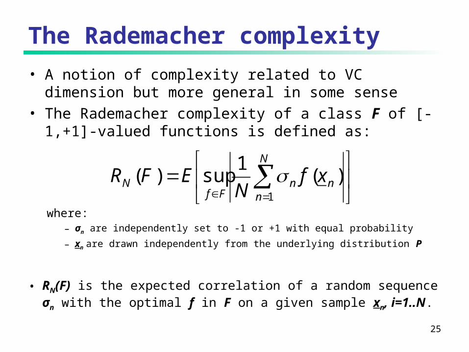
The Rademacher complexity

• A notion of complexity related to VC dimension but more general in some sense

• The Rademacher complexity of a class F of [-1,+1]-valued functions is defined as:

N

nnn

FfN xf

NEFR

1

)(1

sup)(

where: – σn are independently set to -1 or +1 with equal probability

– xn are drawn independently from the underlying distribution P

• RN(F) is the expected correlation of a random sequence σn with the optimal f in F on a given sample xn, i=1..N.

26

The margin-based bound

Theorem 3

Let F be a class of [-1,+1]-valued functions. Then, for every

f in F with probability at least 1-δ:

N

FRfLfyP N

2

log)(4)(ˆ))sign((

2

Note that:

NFVCFRN /)()(

27

Application to boosting

• In boosting the considered hypothesis space is:

)()( )( t1Hhxhαxf:fHcoF

T

t ttT

• The Rademacher complexity of F does not depend on T:

)())(()( HRHcoRFR NTNN

• The generalization bound does not depend on T!

• Whereas the VC dimension of F is dependent on T:

)(log)( HVCTTFVC

28

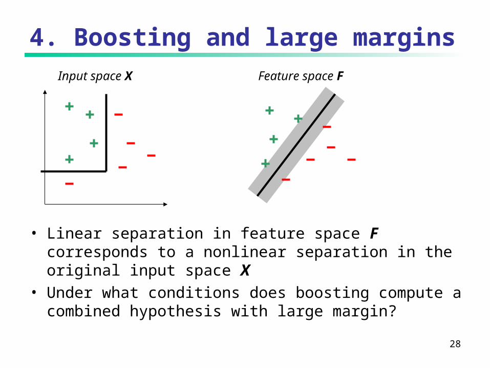
4. Boosting and large marginsInput space X Feature space F

• Linear separation in feature space F corresponds to a nonlinear separation in the original input space X

• Under what conditions does boosting compute a combined hypothesis with large margin?

29

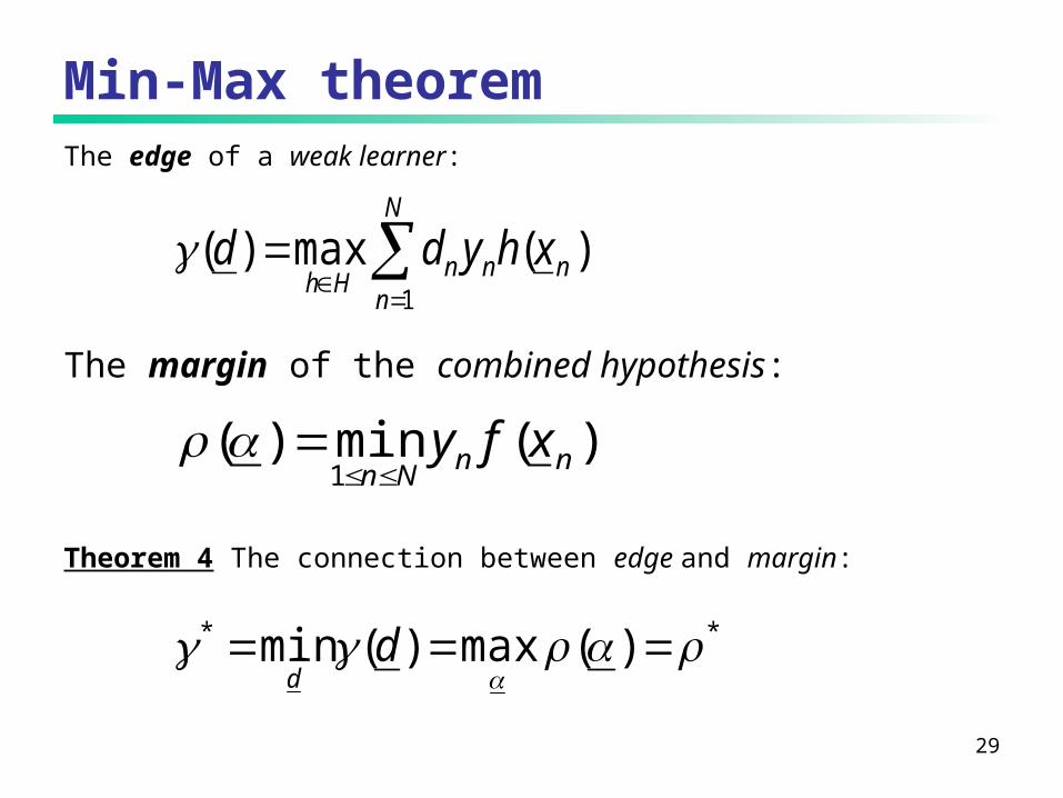
Min-Max theoremThe edge of a weak learner:

)(max)(1

nn

N

nn

Hhxhydd

The margin of the combined hypothesis:

)(min)(1

nnNn

xfy

Theorem 4 The connection between edge and margin:

** )(max)(min

dd

30

Adaboostr algorithm (Breiman 1997)Rule for choosing hypothesis weight:

r

r

t

tt

1

1log

2

1

1

1log

2

1

2

** r

If γ* > r, it guarantees a margin ρ:

where γ* is the minimum edge of hypotheses ht.

31

Achieving the optimal margin bound• Arc-GV

– Choose rt based on the margin achieved so far by the combined hypothesis:

– Convergence rate to maximum margin is not known

• Marginal Adaboost– Run Adaboostr and measure achieved margin ρ

– If ρ < r, then run Adaboostr with a decreased r

– Otherwise run Adaboostr with an increased r

– Converges fast to the maximum margin

))(min,max( 11

1 ntnNn

tt xfyrr

32

Summary

• Boosting takes a weak learner and converts it to a strong one

• Works by asymptotically minimizing the empirical error

• Effectively maximizes the margin of the combined hypothesis

• Obeys “low” generalization error bound under the “luckiness” assumption