INTRODUCTION TO BAYESIAN ANALYSIS · MCMC methods Model checking and comparison Hierarchical and...
246
Introduction to Bayesian analysis, autumn 2013 University of Tampere – 1 / 130 INTRODUCTION TO BAYESIAN ANALYSIS Arto Luoma University of Tampere, Finland Autumn 2014
Transcript of INTRODUCTION TO BAYESIAN ANALYSIS · MCMC methods Model checking and comparison Hierarchical and...

Introduction to Bayesian analysis, autumn 2013 University of Tampere – 1 / 130
INTRODUCTION TO BAYESIAN ANALYSIS
Arto LuomaUniversity of Tampere, Finland
Autumn 2014
Who was Thomas Bayes?
Basic concepts
Single-parametermodels
Hypothesistesting
Simplemultiparametermodels
Markov chains
MCMC methods
Model checkingand comparison
Hierarchical andregressionmodels
Categorical data
Introduction to Bayesian analysis, autumn 2013 University of Tampere – 2 / 130
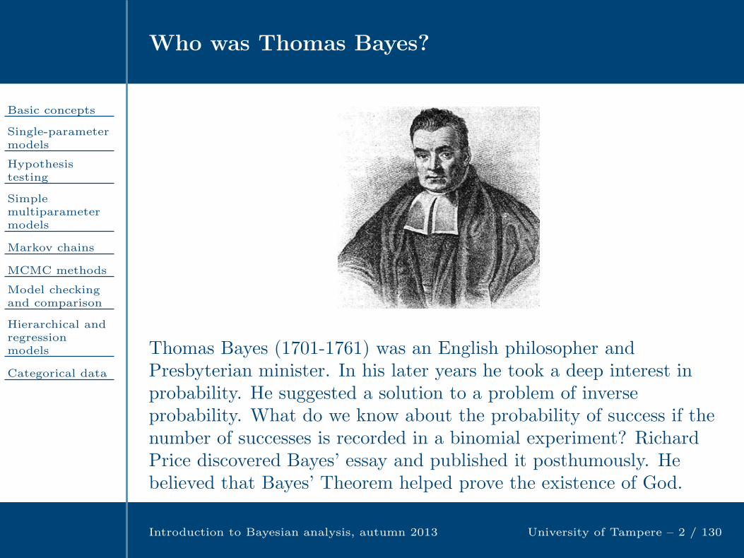
Thomas Bayes (1701-1761) was an English philosopher andPresbyterian minister. In his later years he took a deep interest inprobability. He suggested a solution to a problem of inverseprobability. What do we know about the probability of success if thenumber of successes is recorded in a binomial experiment? RichardPrice discovered Bayes’ essay and published it posthumously. Hebelieved that Bayes’ Theorem helped prove the existence of God.

Bayesian paradigm
Basic concepts
Single-parametermodels
Hypothesistesting
Simplemultiparametermodels
Markov chains
MCMC methods
Model checkingand comparison
Hierarchical andregressionmodels
Categorical data
Introduction to Bayesian analysis, autumn 2013 University of Tampere – 3 / 130
Bayesian paradigm:
posterior information = prior information + data information
More formally:p(θ|y) ∝ p(θ)p(y|θ),
where ∝ is a symbol for proportionality, θ is an unknownparameter, y is data, and p(θ), p(θ|y) and p(y|θ) are the densityfunctions of the prior, posterior and sampling distributions,respectively.
In Bayesian inference, the unknown parameter θ is consideredstochastic, unlike in classical inference. The distributions p(θ)and p(θ|y) express uncertainty about the exact value of θ. Thedensity of data, p(y|θ), provides information from the data. Itis called a likelihood function when considered a function of θ.
Software for Bayesian Statistics
Basic concepts
Single-parametermodels
Hypothesistesting
Simplemultiparametermodels
Markov chains
MCMC methods
Model checkingand comparison
Hierarchical andregressionmodels
Categorical data
Introduction to Bayesian analysis, autumn 2013 University of Tampere – 4 / 130
In this course we use the R and BUGS programming languages.BUGS stands for Bayesian inference Using Gibbs Sampling.Gibbs sampling was the computational technique first adoptedfor Bayesian analysis. The goal of the BUGS project is toseparate the ”knowledge base” from the ”inference machine”used to draw conclusions. BUGS language is able to describecomplex models using very limited syntax.
There are three widely used BUGS implementations:WinBUGS, OpenBUGS and JAGS. Both WinBUGS andOpenBUGS have a Windows GUI. Further, each engine can becontrolled from R. In this course we introduce rjags, the Rinterface to JAGS.
Contents of the course
Basic concepts
Single-parametermodels
Hypothesistesting
Simplemultiparametermodels
Markov chains
MCMC methods
Model checkingand comparison
Hierarchical andregressionmodels
Categorical data
Introduction to Bayesian analysis, autumn 2013 University of Tampere – 5 / 130
Basic concepts
Single-parameter models
Hypothesis testing
Simple multiparameter models
Markov chains
MCMC methods
Model checking and comparison
Hierarchical and regression models
Categorical data
Basic concepts
Basic concepts
Bayes’ theorem
Example
Prior andposteriordistributions
Example 1
Example 2
Decision theory
Bayes estimators
Example 1
Example 2
Conjugate priors
Noninformativepriors
Intervals
Prediction
Single-parametermodels
Hypothesistesting
Simplemultiparametermodels
Markov chains
MCMC methods
Model checkingand comparison
Introduction to Bayesian analysis, autumn 2013 University of Tampere – 6 / 130

Bayes’ theorem
Basic concepts
Bayes’ theorem
Example
Prior andposteriordistributions
Example 1
Example 2
Decision theory
Bayes estimators
Example 1
Example 2
Conjugate priors
Noninformativepriors
Intervals
Prediction
Single-parametermodels
Hypothesistesting
Simplemultiparametermodels
Markov chains
MCMC methods
Model checkingand comparison
Introduction to Bayesian analysis, autumn 2013 University of Tampere – 7 / 130
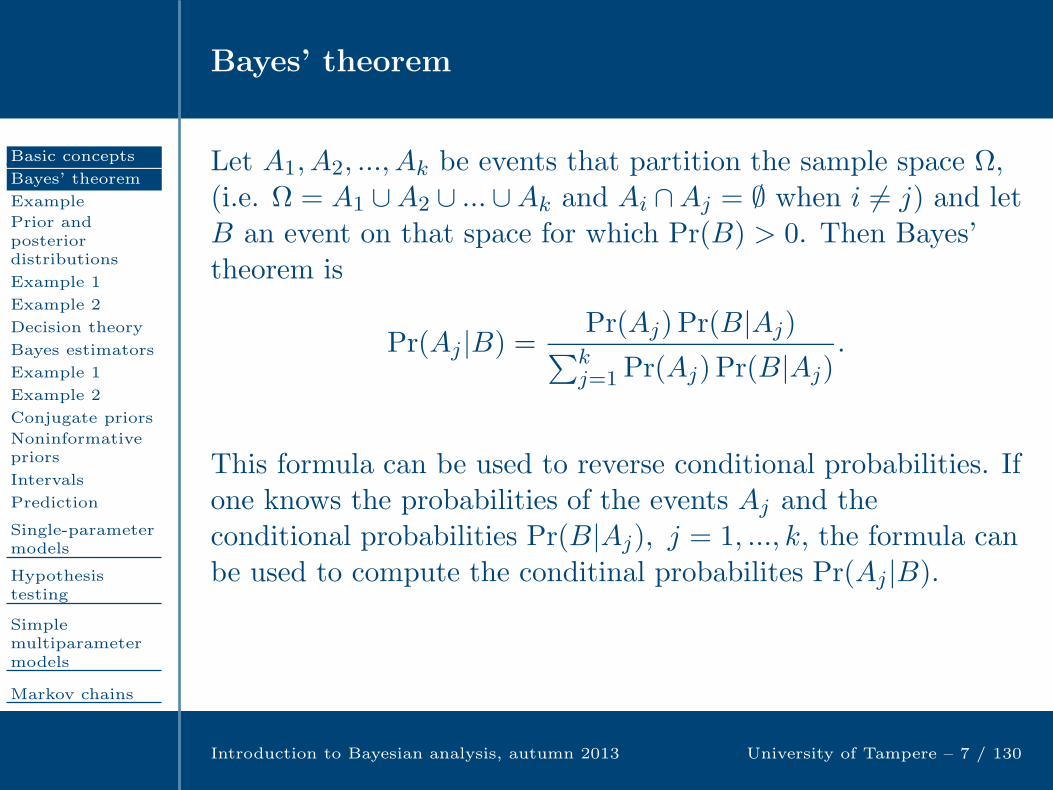
Let A1, A2, ..., Ak be events that partition the sample space Ω,(i.e. Ω = A1 ∪A2 ∪ ...∪Ak and Ai ∩Aj = ∅ when i 6= j) and letB an event on that space for which Pr(B) > 0. Then Bayes’theorem is
Pr(Aj |B) =Pr(Aj) Pr(B|Aj)∑kj=1 Pr(Aj) Pr(B|Aj)
.
Bayes’ theorem
Basic concepts
Bayes’ theorem
Example
Prior andposteriordistributions
Example 1
Example 2
Decision theory
Bayes estimators
Example 1
Example 2
Conjugate priors
Noninformativepriors
Intervals
Prediction
Single-parametermodels
Hypothesistesting
Simplemultiparametermodels
Markov chains
MCMC methods
Model checkingand comparison
Introduction to Bayesian analysis, autumn 2013 University of Tampere – 7 / 130
Let A1, A2, ..., Ak be events that partition the sample space Ω,(i.e. Ω = A1 ∪A2 ∪ ...∪Ak and Ai ∩Aj = ∅ when i 6= j) and letB an event on that space for which Pr(B) > 0. Then Bayes’theorem is
Pr(Aj |B) =Pr(Aj) Pr(B|Aj)∑kj=1 Pr(Aj) Pr(B|Aj)
.
This formula can be used to reverse conditional probabilities. Ifone knows the probabilities of the events Aj and theconditional probabilities Pr(B|Aj), j = 1, ..., k, the formula canbe used to compute the conditinal probabilites Pr(Aj |B).
Example (Diagnostic tests)
Basic concepts
Bayes’ theorem
Example
Prior andposteriordistributions
Example 1
Example 2
Decision theory
Bayes estimators
Example 1
Example 2
Conjugate priors
Noninformativepriors
Intervals
Prediction
Single-parametermodels
Hypothesistesting
Simplemultiparametermodels
Markov chains
MCMC methods
Model checkingand comparison
Introduction to Bayesian analysis, autumn 2013 University of Tampere – 8 / 130
A disease occurs with prevalence γ in population, and θindicates that an individual has the disease. HencePr(θ = 1) = γ, Pr(θ = 0) = 1− γ. A diagnostic test gives aresult Y , whose distribution function is F1(y) for a diseasedindividual and F0(y) otherwise. The most common type of testdeclares that a person is diseased if Y > y0, where y0 is fixed onthe basis of past data.

Example (Diagnostic tests)
Basic concepts
Bayes’ theorem
Example
Prior andposteriordistributions
Example 1
Example 2
Decision theory
Bayes estimators
Example 1
Example 2
Conjugate priors
Noninformativepriors
Intervals
Prediction
Single-parametermodels
Hypothesistesting
Simplemultiparametermodels
Markov chains
MCMC methods
Model checkingand comparison
Introduction to Bayesian analysis, autumn 2013 University of Tampere – 8 / 130
A disease occurs with prevalence γ in population, and θindicates that an individual has the disease. HencePr(θ = 1) = γ, Pr(θ = 0) = 1− γ. A diagnostic test gives aresult Y , whose distribution function is F1(y) for a diseasedindividual and F0(y) otherwise. The most common type of testdeclares that a person is diseased if Y > y0, where y0 is fixed onthe basis of past data. The probability that a person isdiseased, given a positive test result, is
Pr(θ = 1|Y > y0)
=γ[1− F1(y0)]
γ[1− F1(y0)] + (1− γ)[1− F0(y0)].
This is sometimes called the positive predictive value of test. Itssensitivity and specifity are 1− F1(y0) and F0(y0).
(Example from Davison, 2003).

Prior and posterior distributions
Basic concepts
Bayes’ theorem
Example
Prior andposteriordistributions
Example 1
Example 2
Decision theory
Bayes estimators
Example 1
Example 2
Conjugate priors
Noninformativepriors
Intervals
Prediction
Single-parametermodels
Hypothesistesting
Simplemultiparametermodels
Markov chains
MCMC methods
Model checkingand comparison
Introduction to Bayesian analysis, autumn 2013 University of Tampere – 9 / 130
In a more general case, θ can take a finite number of values,labelled 1, ..., k. We can assign to these values probabilitesp1, ..., pk which express our beliefs about θ before we haveaccess to the data. The data y are assumed to be the observedvalue of a (multidimensional) random variable Y , and p(y|θ)the density of y given θ (the likelihood function).

Prior and posterior distributions
Basic concepts
Bayes’ theorem
Example
Prior andposteriordistributions
Example 1
Example 2
Decision theory
Bayes estimators
Example 1
Example 2
Conjugate priors
Noninformativepriors
Intervals
Prediction
Single-parametermodels
Hypothesistesting
Simplemultiparametermodels
Markov chains
MCMC methods
Model checkingand comparison
Introduction to Bayesian analysis, autumn 2013 University of Tampere – 9 / 130
In a more general case, θ can take a finite number of values,labelled 1, ..., k. We can assign to these values probabilitesp1, ..., pk which express our beliefs about θ before we haveaccess to the data. The data y are assumed to be the observedvalue of a (multidimensional) random variable Y , and p(y|θ)the density of y given θ (the likelihood function). Then theconditional probabilites
Pr(θ = j|Y = y) =pjp(y|θ = j)
∑ki=1 pip(y|θ = i)
, j = 1, ..., k,
summarize our beliefs about θ after we have observed Y .
The unconditional probabilities p1, ..., pk are called prior
probablities and Pr(θ = 1|Y = y), ...,Pr(θ = k|Y = y) are calledposterior probabilites of θ.
Prior and posterior distributions (2)
Basic concepts
Bayes’ theorem
Example
Prior andposteriordistributions
Example 1
Example 2
Decision theory
Bayes estimators
Example 1
Example 2
Conjugate priors
Noninformativepriors
Intervals
Prediction
Single-parametermodels
Hypothesistesting
Simplemultiparametermodels
Markov chains
MCMC methods
Model checkingand comparison
Introduction to Bayesian analysis, autumn 2013 University of Tampere – 10 / 130
When θ can get values continuosly on some interval, we canexpress our beliefs about it with a prior density p(θ). After wehave obtained the data y, our beliefs about θ are contained inthe conditional density,
p(θ|y) = p(θ)p(y|θ)∫p(θ)p(y|θ)dθ , (1)
called posterior density.
Since θ is integrated out in the denominator, it can beconsidered as a constant with respect to θ. Therefore, theBayes’ formula in (1) is often written as
p(θ|y) ∝ p(θ)p(y|θ), (2)
which denotes that p(θ|y) is proportional to p(θ)p(y|θ).

Example 1 (Introducing a New Drug in the Market)
Basic concepts
Bayes’ theorem
Example
Prior andposteriordistributions
Example 1
Example 2
Decision theory
Bayes estimators
Example 1
Example 2
Conjugate priors
Noninformativepriors
Intervals
Prediction
Single-parametermodels
Hypothesistesting
Simplemultiparametermodels
Markov chains
MCMC methods
Model checkingand comparison
Introduction to Bayesian analysis, autumn 2013 University of Tampere – 11 / 130
A drug company would like to introduce a drug to reduce acidindigestion. It is desirable to estimate θ, the proportion of themarket share that this drug will capture. The companyinterviews n people and Y of them say that they will buy thedrug. In the non-Bayesian analysis θ ∈ [0, 1] and Y ∼ Bin(n, θ).
We know that θ = Y/n is a very good estimator of θ. It isunbiased, consistent and minimum variance unbiased.Moreover, it is also the maximum likelihood estimator (MLE),and thus asymptotically normal.
A Bayesian may look at the past performance of new drugs ofthis type. If in the past new drugs tend to capture a proportionbetween say .05 and .15 of the market, and if all values inbetween are assumed equally likely, then θ ∼ Unif(.05, .15).
(Example from Rohatgi, 2003).

Example 1 (continued)
Basic concepts
Bayes’ theorem
Example
Prior andposteriordistributions
Example 1
Example 2
Decision theory
Bayes estimators
Example 1
Example 2
Conjugate priors
Noninformativepriors
Intervals
Prediction
Single-parametermodels
Hypothesistesting
Simplemultiparametermodels
Markov chains
MCMC methods
Model checkingand comparison
Introduction to Bayesian analysis, autumn 2013 University of Tampere – 12 / 130
Thus, the prior distribution is given by
p(θ) =
1/(0.15− 0.05) = 10, 0.05 ≤ θ ≤ 0.150, otherwise.
and the likelihood function by
p(y|θ) =(n
y
)θy(1− θ)n−y.
The posterior distribution is
p(θ|y) = p(θ)p(y|θ)∫p(θ)p(y|θ)dθ =
θy(1−θ)n−y
∫ 0.150.05 θy(1−θ)n−ydθ
0.05 ≤ θ ≤ 0.15
0, otherwise.
Example 1 (continued)
Basic concepts
Bayes’ theorem
Example
Prior andposteriordistributions
Example 1
Example 2
Decision theory
Bayes estimators
Example 1
Example 2
Conjugate priors
Noninformativepriors
Intervals
Prediction
Single-parametermodels
Hypothesistesting
Simplemultiparametermodels
Markov chains
MCMC methods
Model checkingand comparison
Introduction to Bayesian analysis, autumn 2013 University of Tampere – 13 / 130
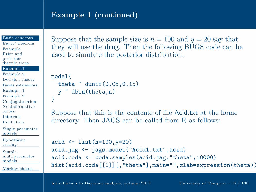
Suppose that the sample size is n = 100 and y = 20 say thatthey will use the drug. Then the following BUGS code can beused to simulate the posterior distribution.
model
theta ~ dunif(0.05,0.15)
y ~ dbin(theta,n)
Suppose that this is the contents of file Acid.txt at the homedirectory. Then JAGS can be called from R as follows:
acid <- list(n=100,y=20)
acid.jag <- jags.model("Acid1.txt",acid)
acid.coda <- coda.samples(acid.jag,"theta",10000)
hist(acid.coda[[1]][,"theta"],main="",xlab=expression(theta))

Example 1 (continued)
Basic concepts
Bayes’ theorem
Example
Prior andposteriordistributions
Example 1
Example 2
Decision theory
Bayes estimators
Example 1
Example 2
Conjugate priors
Noninformativepriors
Intervals
Prediction
Single-parametermodels
Hypothesistesting
Simplemultiparametermodels
Markov chains
MCMC methods
Model checkingand comparison
Introduction to Bayesian analysis, autumn 2013 University of Tampere – 14 / 130
θ
Fre
qu
en
cy
0.08 0.10 0.12 0.14
05
00
10
00
15
00
20
00
25
00
Figure 1: Market share of a new drug: Simulations from theposterior distribution of θ.

Example 2 (Diseased White Pine Trees.)
Basic concepts
Bayes’ theorem
Example
Prior andposteriordistributions
Example 1
Example 2
Decision theory
Bayes estimators
Example 1
Example 2
Conjugate priors
Noninformativepriors
Intervals
Prediction
Single-parametermodels
Hypothesistesting
Simplemultiparametermodels
Markov chains
MCMC methods
Model checkingand comparison
Introduction to Bayesian analysis, autumn 2013 University of Tampere – 15 / 130
White pine is one of the best known species of pines in thenortheastern United States and Canada. White pine issusceptible to blister rust, which develops cankers on the bark.These cankers swell, resulting in death of twigs and small trees.A forester wishes to estimate the average number of diseasedpine trees per acre in a forest.
The number of diseased trees per acre can be modeled by aPoisson distribution with mean θ. Since θ changes from area toarea, the forester believes that θ ∼ Exp(λ). Thus,
p(θ) = (1/λ)e−θ/λ, if θ > 0, and 0 elsewhere
The forester takes a random sample of size n from n different
one-acre plots.
(Example from Rohatgi, 2003).

Example 2 (continued)
Basic concepts
Bayes’ theorem
Example
Prior andposteriordistributions
Example 1
Example 2
Decision theory
Bayes estimators
Example 1
Example 2
Conjugate priors
Noninformativepriors
Intervals
Prediction
Single-parametermodels
Hypothesistesting
Simplemultiparametermodels
Markov chains
MCMC methods
Model checkingand comparison
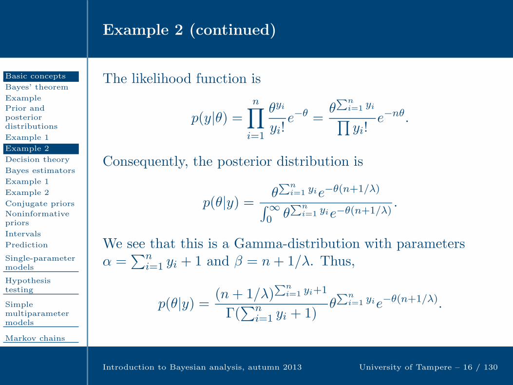
Introduction to Bayesian analysis, autumn 2013 University of Tampere – 16 / 130
The likelihood function is
p(y|θ) =n∏
i=1
θyi
yi!e−θ =
θ∑n
i=1 yi∏yi!
e−nθ.
Example 2 (continued)
Basic concepts
Bayes’ theorem
Example
Prior andposteriordistributions
Example 1
Example 2
Decision theory
Bayes estimators
Example 1
Example 2
Conjugate priors
Noninformativepriors
Intervals
Prediction
Single-parametermodels
Hypothesistesting
Simplemultiparametermodels
Markov chains
MCMC methods
Model checkingand comparison
Introduction to Bayesian analysis, autumn 2013 University of Tampere – 16 / 130
The likelihood function is
p(y|θ) =n∏
i=1
θyi
yi!e−θ =
θ∑n
i=1 yi∏yi!
e−nθ.
Consequently, the posterior distribution is
p(θ|y) = θ∑n
i=1 yie−θ(n+1/λ)
∫∞0 θ
∑ni=1 yie−θ(n+1/λ)
.
We see that this is a Gamma-distribution with parametersα =
∑ni=1 yi + 1 and β = n+ 1/λ.
Example 2 (continued)
Basic concepts
Bayes’ theorem
Example
Prior andposteriordistributions
Example 1
Example 2
Decision theory
Bayes estimators
Example 1
Example 2
Conjugate priors
Noninformativepriors
Intervals
Prediction
Single-parametermodels
Hypothesistesting
Simplemultiparametermodels
Markov chains
MCMC methods
Model checkingand comparison
Introduction to Bayesian analysis, autumn 2013 University of Tampere – 16 / 130
The likelihood function is
p(y|θ) =n∏
i=1
θyi
yi!e−θ =
θ∑n
i=1 yi∏yi!
e−nθ.
Consequently, the posterior distribution is
p(θ|y) = θ∑n
i=1 yie−θ(n+1/λ)
∫∞0 θ
∑ni=1 yie−θ(n+1/λ)
.
We see that this is a Gamma-distribution with parametersα =
∑ni=1 yi + 1 and β = n+ 1/λ. Thus,
p(θ|y) = (n+ 1/λ)∑n
i=1 yi+1
Γ(∑n
i=1 yi + 1)θ∑n
i=1 yie−θ(n+1/λ).

Statistical decision theory
Basic concepts
Bayes’ theorem
Example
Prior andposteriordistributions
Example 1
Example 2
Decision theory
Bayes estimators
Example 1
Example 2
Conjugate priors
Noninformativepriors
Intervals
Prediction
Single-parametermodels
Hypothesistesting
Simplemultiparametermodels
Markov chains
MCMC methods
Model checkingand comparison
Introduction to Bayesian analysis, autumn 2013 University of Tampere – 17 / 130
The outcome of a Bayesian analysis is the posteriordistribution, which combines the prior information and theinformation from data. However, sometimes we may want tosummarize the posterior information with a scalar, for examplethe mean, median or mode of the posterior distribution. In thefollowing, we show how the use of scalar estimator can bejustified using statistical decision theory.
Let L(θ, θ) denote the loss function which gives the cost ofusing θ = θ(y) as an estimate for θ. We define that θ is a Bayes
estimate of θ if it minimizes the posterior expected loss
E[L(θ, θ)|y] =∫L(θ, θ)p(θ|y)dθ.
Statistical decision theory (continued)
Basic concepts
Bayes’ theorem
Example
Prior andposteriordistributions
Example 1
Example 2
Decision theory
Bayes estimators
Example 1
Example 2
Conjugate priors
Noninformativepriors
Intervals
Prediction
Single-parametermodels
Hypothesistesting
Simplemultiparametermodels
Markov chains
MCMC methods
Model checkingand comparison
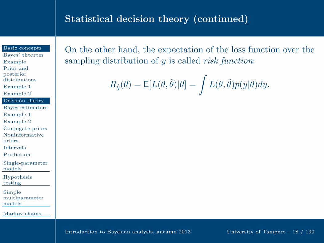
Introduction to Bayesian analysis, autumn 2013 University of Tampere – 18 / 130
On the other hand, the expectation of the loss function over thesampling distribution of y is called risk function:
Rθ(θ) = E[L(θ, θ)|θ] =∫L(θ, θ)p(y|θ)dy.

Statistical decision theory (continued)
Basic concepts
Bayes’ theorem
Example
Prior andposteriordistributions
Example 1
Example 2
Decision theory
Bayes estimators
Example 1
Example 2
Conjugate priors
Noninformativepriors
Intervals
Prediction
Single-parametermodels
Hypothesistesting
Simplemultiparametermodels
Markov chains
MCMC methods
Model checkingand comparison
Introduction to Bayesian analysis, autumn 2013 University of Tampere – 18 / 130
On the other hand, the expectation of the loss function over thesampling distribution of y is called risk function:
Rθ(θ) = E[L(θ, θ)|θ] =∫L(θ, θ)p(y|θ)dy.
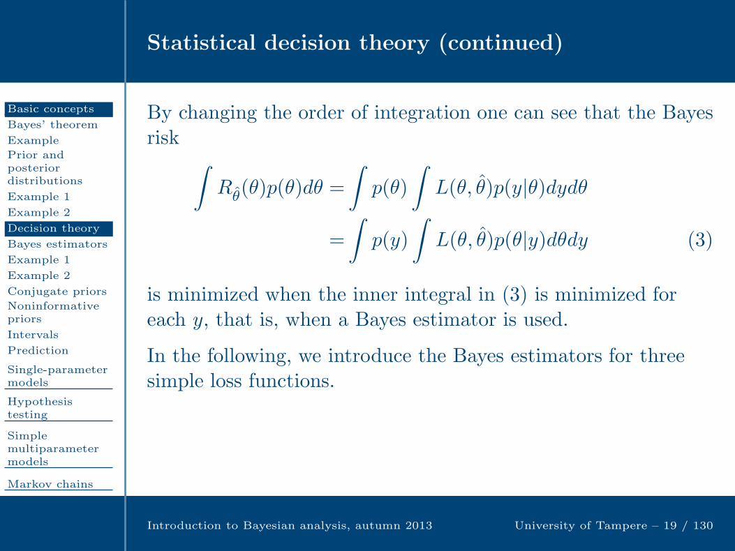
Further, the expectation of the risk function over the priordistribution of θ,
E[Rθ(θ)] =
∫Rθ(θ)p(θ)dθ,
is called Bayes risk.

Statistical decision theory (continued)
Basic concepts
Bayes’ theorem
Example
Prior andposteriordistributions
Example 1
Example 2
Decision theory
Bayes estimators
Example 1
Example 2
Conjugate priors
Noninformativepriors
Intervals
Prediction
Single-parametermodels
Hypothesistesting
Simplemultiparametermodels
Markov chains
MCMC methods
Model checkingand comparison
Introduction to Bayesian analysis, autumn 2013 University of Tampere – 19 / 130
By changing the order of integration one can see that the Bayesrisk
∫Rθ(θ)p(θ)dθ =
∫p(θ)
∫L(θ, θ)p(y|θ)dydθ
=
∫p(y)
∫L(θ, θ)p(θ|y)dθdy (3)
is minimized when the inner integral in (3) is minimized foreach y, that is, when a Bayes estimator is used.
In the following, we introduce the Bayes estimators for threesimple loss functions.
Bayes estimators: zero-one loss function
Basic concepts
Bayes’ theorem
Example
Prior andposteriordistributions
Example 1
Example 2
Decision theory
Bayes estimators
Example 1
Example 2
Conjugate priors
Noninformativepriors
Intervals
Prediction
Single-parametermodels
Hypothesistesting
Simplemultiparametermodels
Markov chains
MCMC methods
Model checkingand comparison
Introduction to Bayesian analysis, autumn 2013 University of Tampere – 20 / 130
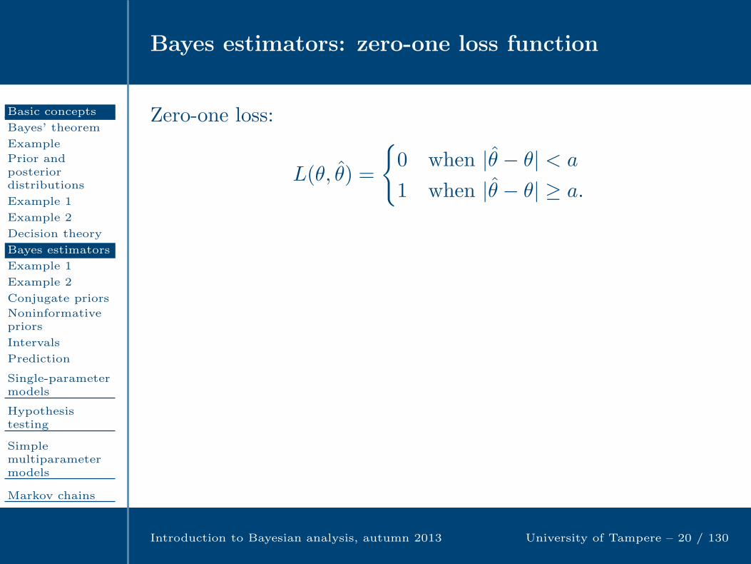
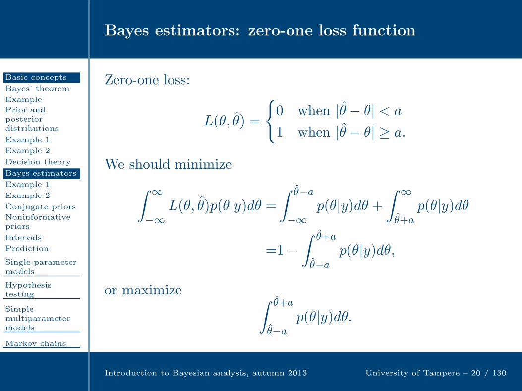
Zero-one loss:
L(θ, θ) =
0 when |θ − θ| < a
1 when |θ − θ| ≥ a.

Bayes estimators: zero-one loss function
Basic concepts
Bayes’ theorem
Example
Prior andposteriordistributions
Example 1
Example 2
Decision theory
Bayes estimators
Example 1
Example 2
Conjugate priors
Noninformativepriors
Intervals
Prediction
Single-parametermodels
Hypothesistesting
Simplemultiparametermodels
Markov chains
MCMC methods
Model checkingand comparison
Introduction to Bayesian analysis, autumn 2013 University of Tampere – 20 / 130
Zero-one loss:
L(θ, θ) =
0 when |θ − θ| < a
1 when |θ − θ| ≥ a.
We should minimize
∫ ∞
−∞L(θ, θ)p(θ|y)dθ =
∫ θ−a
−∞p(θ|y)dθ +
∫ ∞
θ+ap(θ|y)dθ
=1−∫ θ+a
θ−ap(θ|y)dθ,
or maximize ∫ θ+a
θ−ap(θ|y)dθ.
Bayes estimators: absolute error loss and quadraticloss function
Basic concepts
Bayes’ theorem
Example
Prior andposteriordistributions
Example 1
Example 2
Decision theory
Bayes estimators
Example 1
Example 2
Conjugate priors
Noninformativepriors
Intervals
Prediction
Single-parametermodels
Hypothesistesting
Simplemultiparametermodels
Markov chains
MCMC methods
Model checkingand comparison
Introduction to Bayesian analysis, autumn 2013 University of Tampere – 21 / 130
If p(θ|y) is unimodal, maximization is achieved by choosing θ tobe the midpoint of the interval of length 2a for which p(θ|y) hasthe same value at both ends. If we let a→ 0, then θ tends tothe mode of the posterior distribution. This equals the MLE ifp(θ) is ’flat’.
Absolute error loss: L(θ, θ) = |θ − θ|. In general, if X is arandom variable, then the expectation E(|X − d|) is minimizedby choosing d to be the median of the distribution of X. Thus,the Bayes estimate of θ is the posterior median.
Quadratic loss function: L(θ, θ) = (θ − θ)2. In general, if X is arandom variable, then the expectation E[(X − d)2] is minimizedby choosing d to be the mean of the distribution of X. Thus,the Bayes estimate of θ is the posterior mean.
Bayes estimators: Example 1 (cont)
Basic concepts
Bayes’ theorem
Example
Prior andposteriordistributions
Example 1
Example 2
Decision theory
Bayes estimators
Example 1
Example 2
Conjugate priors
Noninformativepriors
Intervals
Prediction
Single-parametermodels
Hypothesistesting
Simplemultiparametermodels
Markov chains
MCMC methods
Model checkingand comparison
Introduction to Bayesian analysis, autumn 2013 University of Tampere – 22 / 130
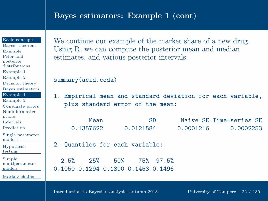
We continue our example of the market share of a new drug.Using R, we can compute the posterior mean and medianestimates, and various posterior intervals:
summary(acid.coda)
1. Empirical mean and standard deviation for each variable,
plus standard error of the mean:
Mean SD Naive SE Time-series SE
0.1357622 0.0121584 0.0001216 0.0002253
2. Quantiles for each variable:
2.5% 25% 50% 75% 97.5%
0.1050 0.1294 0.1390 0.1453 0.1496

Bayes estimators: Example 1 (cont)
Basic concepts
Bayes’ theorem
Example
Prior andposteriordistributions
Example 1
Example 2
Decision theory
Bayes estimators
Example 1
Example 2
Conjugate priors
Noninformativepriors
Intervals
Prediction
Single-parametermodels
Hypothesistesting
Simplemultiparametermodels
Markov chains
MCMC methods
Model checkingand comparison
Introduction to Bayesian analysis, autumn 2013 University of Tampere – 23 / 130
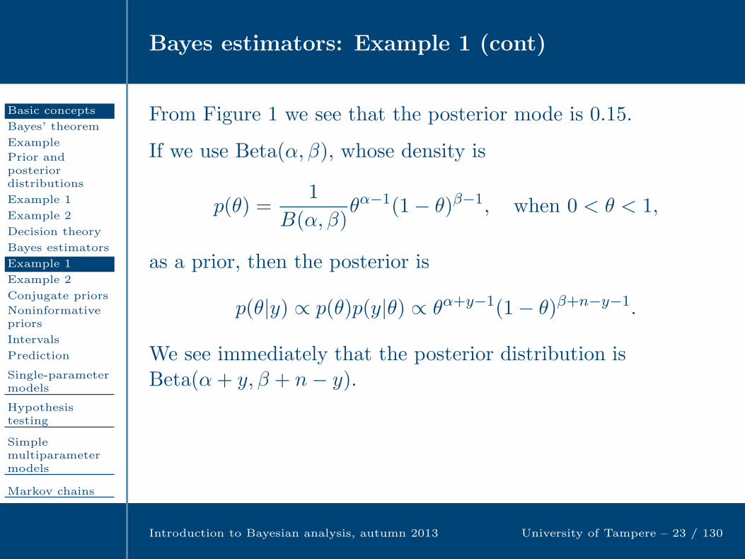
From Figure 1 we see that the posterior mode is 0.15.
Bayes estimators: Example 1 (cont)
Basic concepts
Bayes’ theorem
Example
Prior andposteriordistributions
Example 1
Example 2
Decision theory
Bayes estimators
Example 1
Example 2
Conjugate priors
Noninformativepriors
Intervals
Prediction
Single-parametermodels
Hypothesistesting
Simplemultiparametermodels
Markov chains
MCMC methods
Model checkingand comparison
Introduction to Bayesian analysis, autumn 2013 University of Tampere – 23 / 130
From Figure 1 we see that the posterior mode is 0.15.
If we use Beta(α, β), whose density is
p(θ) =1
B(α, β)θα−1(1− θ)β−1, when 0 < θ < 1,
as a prior, then the posterior is
p(θ|y) ∝ p(θ)p(y|θ) ∝ θα+y−1(1− θ)β+n−y−1.
We see immediately that the posterior distribution isBeta(α+ y, β + n− y).
The posterior mean (Bayes estimator with quadratic loss) is(α+ y)/(α+ β + n). The mode (Bayes estimator with zero-oneloss when a→ 0) is (α+ y − 1)/(α+ β + n− 2), provided thatthe distribution is unimodal.
Bayes estimators: Example 2 (cont)
Basic concepts
Bayes’ theorem
Example
Prior andposteriordistributions
Example 1
Example 2
Decision theory
Bayes estimators
Example 1
Example 2
Conjugate priors
Noninformativepriors
Intervals
Prediction
Single-parametermodels
Hypothesistesting
Simplemultiparametermodels
Markov chains
MCMC methods
Model checkingand comparison
Introduction to Bayesian analysis, autumn 2013 University of Tampere – 24 / 130
We now continue our example of estimating the proportion ofdiseased trees. We derived that the posterior distribution isGamma(
∑ni=1 yi + 1, n+ 1/λ). Thus, the Bayes estimator with
a quadratic loss function is the mean of this distribution,(∑n
i=1 yi + 1)/(n+ 1/λ). However, the mean and mode of agamma distribution do not exist in closed form.
Note that the classical estimate for θ is the sample mean y.
Conjugate prior distribution
Basic concepts
Bayes’ theorem
Example
Prior andposteriordistributions
Example 1
Example 2
Decision theory
Bayes estimators
Example 1
Example 2
Conjugate priors
Noninformativepriors
Intervals
Prediction
Single-parametermodels
Hypothesistesting
Simplemultiparametermodels
Markov chains
MCMC methods
Model checkingand comparison
Introduction to Bayesian analysis, autumn 2013 University of Tampere – 25 / 130
Computations can often be facilitated using conjugate prior
distributions. We say that a prior is conjugate for the likelihoodif the prior and posterior distributions belong to the samefamily. There are conjugate distributions for the exponentialfamily of sampling distributions.
Conjugate priors can be formed with the following simple steps:
1. Write the likelihood function.2. Remove the factors that do not depend on θ.3. Replace the expressions which depend on data with
parameters. Also the sample size n should be replaced.4. Now you have the kernel of the conjugate prior. You can
complement it with the normalizing constant.5. In order to obtain the standard parametrization it may be
necessary to reparametrize.
Example: Poisson likelihood
Basic concepts
Bayes’ theorem
Example
Prior andposteriordistributions
Example 1
Example 2
Decision theory
Bayes estimators
Example 1
Example 2
Conjugate priors
Noninformativepriors
Intervals
Prediction
Single-parametermodels
Hypothesistesting
Simplemultiparametermodels
Markov chains
MCMC methods
Model checkingand comparison
Introduction to Bayesian analysis, autumn 2013 University of Tampere – 26 / 130
Let y = (y1, ...yn) be a sample from Poi(θ). Then the likelihoodis
p(y|θ) =n∏
i=1
θyie−θ
yi!∝ θ
∑yie−nθ.
By replacing∑yi and n, which depend on the data, with the
parameters α1 and α2, we obtain the conjugate prior
p(θ) ∝ θα1e−α2θ,
which is Gamma(α1 + 1, α2) distribution. If we reparametrizethis distribution so that α = α1 + 1 and β = α2 we obtain theprior Gamma(α, β).

Example: Uniform likelihood
Basic concepts
Bayes’ theorem
Example
Prior andposteriordistributions
Example 1
Example 2
Decision theory
Bayes estimators
Example 1
Example 2
Conjugate priors
Noninformativepriors
Intervals
Prediction
Single-parametermodels
Hypothesistesting
Simplemultiparametermodels
Markov chains
MCMC methods
Model checkingand comparison
Introduction to Bayesian analysis, autumn 2013 University of Tampere – 27 / 130
Assume that y = (y1, ..., yn) is a random sample from Unif(0, θ).The the density of a single observation yi is
p(yi|θ) =
1θ 0 ≤ yi ≤ θ,0, otherwise,
and the likelihood of θ is
p(y|θ) =
1θn , 0 ≤ y(1) ≤ ... ≤ y(n) ≤ θ,
0, otherwise,
=1
θnIy(n)≤θ(y) Iy(1)≥0(y),
where IA(y) denotes an indicator function obtaining value 1when y ∈ A and 0 otherwise.

Example: Uniform likelihood (cont)
Basic concepts
Bayes’ theorem
Example
Prior andposteriordistributions
Example 1
Example 2
Decision theory
Bayes estimators
Example 1
Example 2
Conjugate priors
Noninformativepriors
Intervals
Prediction
Single-parametermodels
Hypothesistesting
Simplemultiparametermodels
Markov chains
MCMC methods
Model checkingand comparison
Introduction to Bayesian analysis, autumn 2013 University of Tampere – 28 / 130
Now, by removing the factor Iy(1)≥0(y), which does notdepend on θ, and replacing n and y(n) with parameters weobtain
p(θ) ∝ 1
θαIθ≥β(θ)
=
1θα , when θ ≥ β,0, otherwise.
This is the kernel of the Pareto distribution.

Example: Uniform likelihood (cont)
Basic concepts
Bayes’ theorem
Example
Prior andposteriordistributions
Example 1
Example 2
Decision theory
Bayes estimators
Example 1
Example 2
Conjugate priors
Noninformativepriors
Intervals
Prediction
Single-parametermodels
Hypothesistesting
Simplemultiparametermodels
Markov chains
MCMC methods
Model checkingand comparison
Introduction to Bayesian analysis, autumn 2013 University of Tampere – 28 / 130
Now, by removing the factor Iy(1)≥0(y), which does notdepend on θ, and replacing n and y(n) with parameters weobtain
p(θ) ∝ 1
θαIθ≥β(θ)
=
1θα , when θ ≥ β,0, otherwise.
This is the kernel of the Pareto distribution.The posteriordistribution
p(θ|y) ∝ p(θ)p(y|θ)
∝
1θn+α , when θ ≥ max(β, y(n))
0, otherwise.
is also a Pareto distribution.

Noninformative prior distribution
Basic concepts
Bayes’ theorem
Example
Prior andposteriordistributions
Example 1
Example 2
Decision theory
Bayes estimators
Example 1
Example 2
Conjugate priors
Noninformativepriors
Intervals
Prediction
Single-parametermodels
Hypothesistesting
Simplemultiparametermodels
Markov chains
MCMC methods
Model checkingand comparison
Introduction to Bayesian analysis, autumn 2013 University of Tampere – 29 / 130
When there is no prior information available on the estimatedparameters, noninformative priors can be used. They can alsobe used to find out how an informative prior affects theoutcome of the inference.
The uniform distribution p(θ) ∝ 1 is often used as anoninformative prior. However, this is not fully unproblematic.If the uniform distribution is restricted to an interval, it is not,in fact, noninformative. For example, the prior Unif(0, 1),contains the information that θ is in the interval [0.2, 0.4] withprobability 0.2. This information content becomes obviouswhen a parametric transformation is made. The distribution ofthe transformed parameter is no more uniform.
Noninformative prior distribution (cont)
Basic concepts
Bayes’ theorem
Example
Prior andposteriordistributions
Example 1
Example 2
Decision theory
Bayes estimators
Example 1
Example 2
Conjugate priors
Noninformativepriors
Intervals
Prediction
Single-parametermodels
Hypothesistesting
Simplemultiparametermodels
Markov chains
MCMC methods
Model checkingand comparison
Introduction to Bayesian analysis, autumn 2013 University of Tampere – 30 / 130
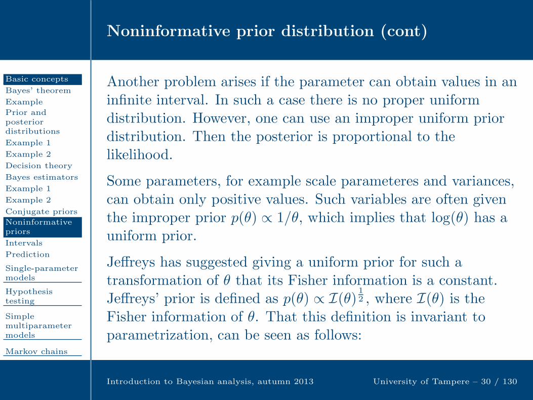
Another problem arises if the parameter can obtain values in aninfinite interval. In such a case there is no proper uniformdistribution. However, one can use an improper uniform priordistribution. Then the posterior is proportional to thelikelihood.
Noninformative prior distribution (cont)
Basic concepts
Bayes’ theorem
Example
Prior andposteriordistributions
Example 1
Example 2
Decision theory
Bayes estimators
Example 1
Example 2
Conjugate priors
Noninformativepriors
Intervals
Prediction
Single-parametermodels
Hypothesistesting
Simplemultiparametermodels
Markov chains
MCMC methods
Model checkingand comparison
Introduction to Bayesian analysis, autumn 2013 University of Tampere – 30 / 130
Another problem arises if the parameter can obtain values in aninfinite interval. In such a case there is no proper uniformdistribution. However, one can use an improper uniform priordistribution. Then the posterior is proportional to thelikelihood.
Some parameters, for example scale parameteres and variances,can obtain only positive values. Such variables are often giventhe improper prior p(θ) ∝ 1/θ, which implies that log(θ) has auniform prior.
Jeffreys has suggested giving a uniform prior for such atransformation of θ that its Fisher information is a constant.Jeffreys’ prior is defined as p(θ) ∝ I(θ) 1
2 , where I(θ) is theFisher information of θ. That this definition is invariant toparametrization, can be seen as follows:

Noninformative prior distribution (cont)
Basic concepts
Bayes’ theorem
Example
Prior andposteriordistributions
Example 1
Example 2
Decision theory
Bayes estimators
Example 1
Example 2
Conjugate priors
Noninformativepriors
Intervals
Prediction
Single-parametermodels
Hypothesistesting
Simplemultiparametermodels
Markov chains
MCMC methods
Model checkingand comparison
Introduction to Bayesian analysis, autumn 2013 University of Tampere – 31 / 130
Let φ = h(θ) be a regular, monotonic transformation of θ, andits inverse transformation θ = h−1(φ). Then the Fisherinformation of φ is
I(φ) =E
[(d log p(y|φ)
dφ
)2∣∣∣∣∣φ]
=E
[(d log p(y|θ = h−1(φ))
dθ
)2∣∣∣∣∣φ] ∣∣∣∣dθ
dφ
∣∣∣∣2
=I(θ)∣∣∣∣dθ
dφ
∣∣∣∣2
.
Thus, I(φ) 12 = I(Θ)
12
∣∣∣ dθdφ∣∣∣.
On the other hand, p(φ) = p(θ)∣∣∣ dθdφ∣∣∣ = I(Θ)
12
∣∣∣ dθdφ∣∣∣, as required.

Jeffreys’ prior: Examples
Basic concepts
Bayes’ theorem
Example
Prior andposteriordistributions
Example 1
Example 2
Decision theory
Bayes estimators
Example 1
Example 2
Conjugate priors
Noninformativepriors
Intervals
Prediction
Single-parametermodels
Hypothesistesting
Simplemultiparametermodels
Markov chains
MCMC methods
Model checkingand comparison
Introduction to Bayesian analysis, autumn 2013 University of Tampere – 32 / 130
Binomial distribution
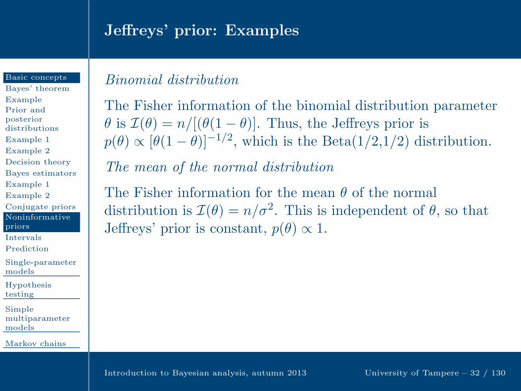
The Fisher information of the binomial distribution parameterθ is I(θ) = n/[(θ(1− θ)]. Thus, the Jeffreys prior isp(θ) ∝ [θ(1− θ)]−1/2, which is the Beta(1/2,1/2) distribution.
Jeffreys’ prior: Examples
Basic concepts
Bayes’ theorem
Example
Prior andposteriordistributions
Example 1
Example 2
Decision theory
Bayes estimators
Example 1
Example 2
Conjugate priors
Noninformativepriors
Intervals
Prediction
Single-parametermodels
Hypothesistesting
Simplemultiparametermodels
Markov chains
MCMC methods
Model checkingand comparison
Introduction to Bayesian analysis, autumn 2013 University of Tampere – 32 / 130
Binomial distribution
The Fisher information of the binomial distribution parameterθ is I(θ) = n/[(θ(1− θ)]. Thus, the Jeffreys prior isp(θ) ∝ [θ(1− θ)]−1/2, which is the Beta(1/2,1/2) distribution.
The mean of the normal distribution
The Fisher information for the mean θ of the normaldistribution is I(θ) = n/σ2. This is independent of θ, so thatJeffreys’ prior is constant, p(θ) ∝ 1.
The variance of the normal distribution
Assume that the variance θ of the normal distribution N(µ, θ)is unknown. Then its Fisher information is I(θ) = n/(2θ2), andJeffreys’ prior p(θ) ∝ 1/θ.
Posterior intervals
Basic concepts
Bayes’ theorem
Example
Prior andposteriordistributions
Example 1
Example 2
Decision theory
Bayes estimators
Example 1
Example 2
Conjugate priors
Noninformativepriors
Intervals
Prediction
Single-parametermodels
Hypothesistesting
Simplemultiparametermodels
Markov chains
MCMC methods
Model checkingand comparison
Introduction to Bayesian analysis, autumn 2013 University of Tampere – 33 / 130
Whe have seen that it is possible to summarize posteriorinformation using point estimators. However, posterior regionsand intervals are usually more useful. We define that a set C isa posterior region of level 1− α for θ if the posterior probabilityof θ belonging to C is 1− α:
Pr(θ ∈ C|y) =∫
Cp(θ|y)dθ = 1− α.
In the case of scalar parameters one can use posterior intervals(credible intervals). An equi-tailed posterior inteval is definedusing quantiles of the posterior. Thus, (θL, θU ) is an100(1− α)% interval if Pr(θ < θL|y) = Pr(θ > θU |y) = α/2.
An advantage of this type of interval is that it is invariant withrespect to one-to-one parameter transformations. Further, it iseasy to compute.

Posterior intervals (cont)
Basic concepts
Bayes’ theorem
Example
Prior andposteriordistributions
Example 1
Example 2
Decision theory
Bayes estimators
Example 1
Example 2
Conjugate priors
Noninformativepriors
Intervals
Prediction
Single-parametermodels
Hypothesistesting
Simplemultiparametermodels
Markov chains
MCMC methods
Model checkingand comparison
Introduction to Bayesian analysis, autumn 2013 University of Tampere – 34 / 130
A posterior region is said to be a highest posterior density
region (HPD region) if the posterior density is larger in allpoints of the region than in any point outside the region. Thistype of region has the smallest possible volume. In a scalarcase, an HPD interval has the smallest length. On the otherhand, the bounds of the interval are not invariant with respectto parameter transformations, and it is not always easy todetermine them.
Example. Cardiac surgery data. Table 1 shows mortality ratesfor cardiac surgery on babies at 12 hospitals. If one wishes toestimate the mortality rate in hospital A, denoted as θA, thesimpliest approach is to assume that the number of deaths y isbinomially distributed with parameters n and θA where n is thenumber of operations in A. Then the MLE is θA = 0, whichsounds too optimistic.

Posterior intervals (cont)
Basic concepts
Bayes’ theorem
Example
Prior andposteriordistributions
Example 1
Example 2
Decision theory
Bayes estimators
Example 1
Example 2
Conjugate priors
Noninformativepriors
Intervals
Prediction
Single-parametermodels
Hypothesistesting
Simplemultiparametermodels
Markov chains
MCMC methods
Model checkingand comparison
Introduction to Bayesian analysis, autumn 2013 University of Tampere – 35 / 130
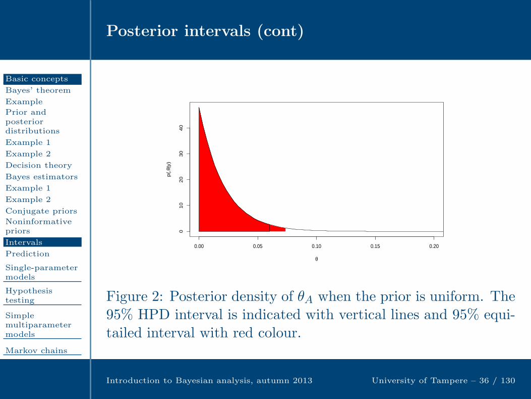
If we give a uniform prior for θA, then the posterior distributionis Beta(1,48), with posterior mean 1/49. The 95% HPD intervalis (0,6.05)% and equi-tailed interval (0.05,7.30)%. Figure 2shows the posterior density. Another approach would use thetotal numbers of deaths and operations in all hospitals.
Table 1: Mortality rates y/n from cardiac surgery in 12 hospitals(Spiegelhalter et. al, BUGS 0.5 Examples Volume 1, Cambridge:MRC Biostatistics Unit, 1996). The numbers of deaths y out ofn operations.
A 0/47 B 18/148 C 8/119 D 46/810E 8/211 F 13/196 G 9/148 H 31/215I 14/207 J 8/97 K 29/256 L 24/360
Posterior intervals (cont)
Basic concepts
Bayes’ theorem
Example
Prior andposteriordistributions
Example 1
Example 2
Decision theory
Bayes estimators
Example 1
Example 2
Conjugate priors
Noninformativepriors
Intervals
Prediction
Single-parametermodels
Hypothesistesting
Simplemultiparametermodels
Markov chains
MCMC methods
Model checkingand comparison
Introduction to Bayesian analysis, autumn 2013 University of Tampere – 36 / 130
0.00 0.05 0.10 0.15 0.20
01
02
03
04
0
θ
p(,
θ|y)
Figure 2: Posterior density of θA when the prior is uniform. The95% HPD interval is indicated with vertical lines and 95% equi-tailed interval with red colour.

Posterior intervals (cont)
Basic concepts
Bayes’ theorem
Example
Prior andposteriordistributions
Example 1
Example 2
Decision theory
Bayes estimators
Example 1
Example 2
Conjugate priors
Noninformativepriors
Intervals
Prediction
Single-parametermodels
Hypothesistesting
Simplemultiparametermodels
Markov chains
MCMC methods
Model checkingand comparison
Introduction to Bayesian analysis, autumn 2013 University of Tampere – 37 / 130
The following BUGS and R codes can be used to compute theequi-tailed and HPD intervals:
model
theta ~ dbeta(1,1)
y ~ dbin(theta,n)
hospital <- list(n=47,y=0)
hospital.jag <- jags.model("Hospital.txt",hospital)
hospital.coda <- coda.samples(hospital.jag,"theta",10000)
summary(hospital.coda)
HPDinterval(hospital.coda)
#Compare with exact upper limit of HPD interval:
qbeta(0.95,1,48)
[1] 0.06050341

Posterior predictive distribution
Basic concepts
Bayes’ theorem
Example
Prior andposteriordistributions
Example 1
Example 2
Decision theory
Bayes estimators
Example 1
Example 2
Conjugate priors
Noninformativepriors
Intervals
Prediction
Single-parametermodels
Hypothesistesting
Simplemultiparametermodels
Markov chains
MCMC methods
Model checkingand comparison
Introduction to Bayesian analysis, autumn 2013 University of Tampere – 38 / 130
If we wish to predict a new observation y on the basis of thesample y = (y1, ...yn), we may use its posterior predictive
distribution. This is defined to be the conditional distributionof y given y:
p(y|y) =∫p(y, θ|y)dθ
=
∫p(y|y, θ)p(θ|y)dθ,
where p(y|y, θ) is the density of the predictive distribution.
It is easy to simulate the posterior predictive distribution.First, draw simulations θ1, ..., θL from the posterior p(θ|y), then,for each i, draw yi from the predictive distribution p(y|y, θi).

Posterior predictive distribution: Example
Basic concepts
Bayes’ theorem
Example
Prior andposteriordistributions
Example 1
Example 2
Decision theory
Bayes estimators
Example 1
Example 2
Conjugate priors
Noninformativepriors
Intervals
Prediction
Single-parametermodels
Hypothesistesting
Simplemultiparametermodels
Markov chains
MCMC methods
Model checkingand comparison
Introduction to Bayesian analysis, autumn 2013 University of Tampere – 39 / 130
Assume that we have a coin with unknown probability θ of ahead. If there occurs y heads among the first n tosses what isthe probability of a head on the next throw?
Let y = 1 (y = 0) indicate the event that the next throw is ahead (tail). If the prior of θ is Beta(α, β), then
p(y|y) =∫ 1
0p(y|y, θ)p(θ|y)dθ
=
∫ 1
0θy(1− θ)1−y θ
α+y−1(1− θ)β+n−y−1
B(α+ y, β + n− y)dθ
=B(α+ y + y, β + n− y − y + 1)
B(α+ y, β + n− y)
=(α+ y)y(β + n− y)1−y
α+ β + n.

Posterior predictive distribution: Example (cont)
Basic concepts
Bayes’ theorem
Example
Prior andposteriordistributions
Example 1
Example 2
Decision theory
Bayes estimators
Example 1
Example 2
Conjugate priors
Noninformativepriors
Intervals
Prediction
Single-parametermodels
Hypothesistesting
Simplemultiparametermodels
Markov chains
MCMC methods
Model checkingand comparison
Introduction to Bayesian analysis, autumn 2013 University of Tampere – 40 / 130
Thus, Pr(y = 1|y) = (α+ y)/(α+ β + n). This tends to thesample proportion y/n as n→ ∞, so that the role of the priorinformation vanishes. If n = 10 and y = 4 and prior parametersα = β = 0.5 (Jeffreys’ prior), the posterior predictivedistribution can be simulated with BUGS as follows:
model
theta ~ dbeta(alpha,beta)
y ~ dbin(theta,n)
ynew ~ dbern(theta)
coin <- list(n=10,y=4,alpha=0.5,beta=0.5)
coin.jag <- jags.model("Coin.txt",coin)
coin.coda <- coda.samples(coin.jag,c("theta","ynew"),10000)
summary(coin.coda)
Single-parameter models
Basic concepts
Single-parametermodelsNormaldistributionPoissondistributionExponentialdistribution
Hypothesistesting
Simplemultiparametermodels
Markov chains
MCMC methods
Model checkingand comparison
Hierarchical andregressionmodels
Categorical data
Introduction to Bayesian analysis, autumn 2013 University of Tampere – 41 / 130
Normal distribution with known variance
Basic concepts
Single-parametermodelsNormaldistributionPoissondistributionExponentialdistribution
Hypothesistesting
Simplemultiparametermodels
Markov chains
MCMC methods
Model checkingand comparison
Hierarchical andregressionmodels
Categorical data
Introduction to Bayesian analysis, autumn 2013 University of Tampere – 42 / 130
Next we will consider some simple single-parameter models. Letus first assume that y = (y1, ...yn) is a sample from a normaldistribution unknown mean θ and known variance σ2. Thelikelihood is then
p(y|θ) =n∏
i=1
1√2πσ2
e−1
2σ2 (yi−θ)2
∝ e−1
2σ2
∑ni=1(yi−θ)2
∝ e−n
2σ2 (θ−y)2 .
By replacing σ2/n with τ20 , and y with µ0, we find a conjugateprior
p(θ) ∝ e− 1
2τ20(θ−µ0)2
,
which is N(µ0, τ20 ).
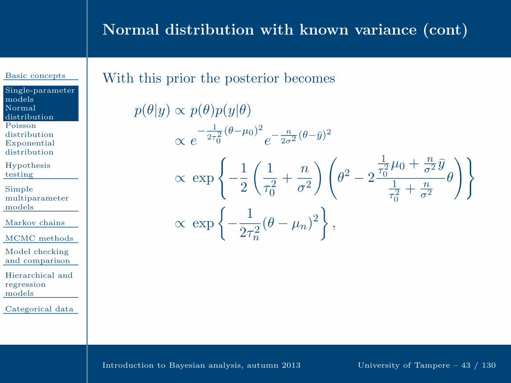
Normal distribution with known variance (cont)
Basic concepts
Single-parametermodelsNormaldistributionPoissondistributionExponentialdistribution
Hypothesistesting
Simplemultiparametermodels
Markov chains
MCMC methods
Model checkingand comparison
Hierarchical andregressionmodels
Categorical data
Introduction to Bayesian analysis, autumn 2013 University of Tampere – 43 / 130
With this prior the posterior becomes
p(θ|y) ∝ p(θ)p(y|θ)
∝ e− 1
2τ20(θ−µ0)2
e−n
2σ2 (θ−y)2
∝ exp
−1
2
(1
τ20+
n
σ2
)(θ2 − 2
1τ20µ0 +
nσ2 y
1τ20
+ nσ2
θ
)
∝ exp
− 1
2τ2n(θ − µn)
2
,
where
µn =
1τ20µ0 +
nσ2 y
1τ20
+ nσ2
and τ2n =
(1
τ20+
n
σ2
)−1
.

Normal distribution with known variance (cont)
Basic concepts
Single-parametermodelsNormaldistributionPoissondistributionExponentialdistribution
Hypothesistesting
Simplemultiparametermodels
Markov chains
MCMC methods
Model checkingand comparison
Hierarchical andregressionmodels
Categorical data
Introduction to Bayesian analysis, autumn 2013 University of Tampere – 44 / 130
Thus, the posterior distribution is N(µn, τ2n).
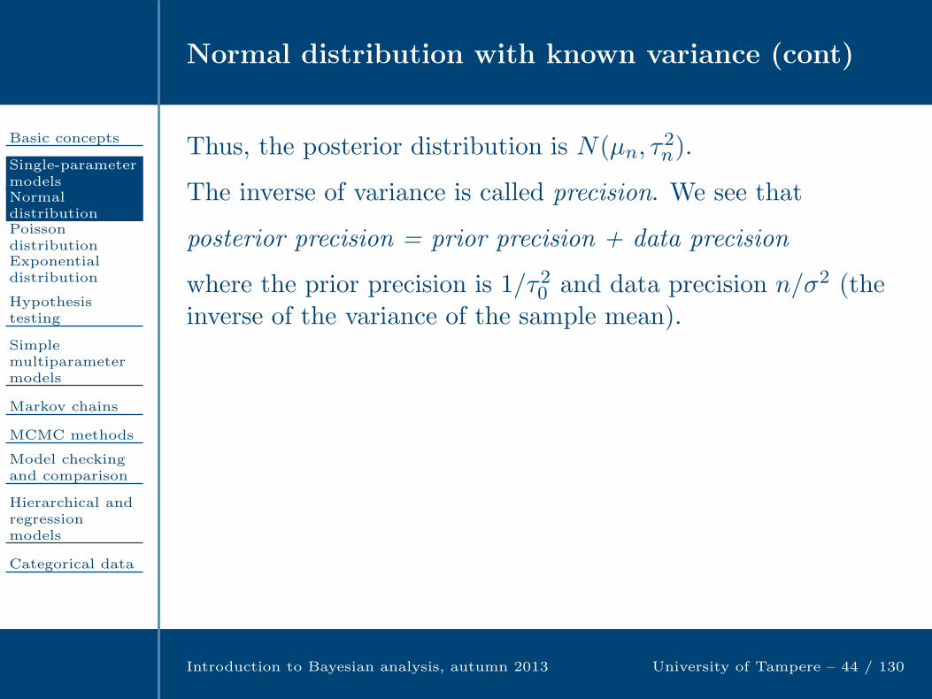
The inverse of variance is called precision. We see that
posterior precision = prior precision + data precision
where the prior precision is 1/τ20 and data precision n/σ2 (theinverse of the variance of the sample mean).
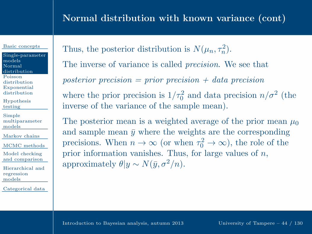
The posterior mean is a weighted average of the prior mean µ0and sample mean y where the weights are the correspondingprecisions. When n→ ∞ (or when τ20 → ∞), the role of theprior information vanishes. Thus, for large values of n,approximately θ|y ∼ N(y, σ2/n).
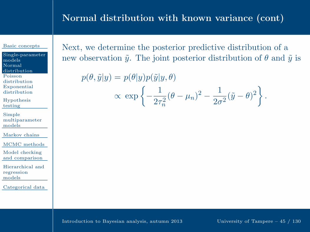
Normal distribution with known variance (cont)
Basic concepts
Single-parametermodelsNormaldistributionPoissondistributionExponentialdistribution
Hypothesistesting
Simplemultiparametermodels
Markov chains
MCMC methods
Model checkingand comparison
Hierarchical andregressionmodels
Categorical data
Introduction to Bayesian analysis, autumn 2013 University of Tampere – 45 / 130
Next, we determine the posterior predictive distribution of anew observation y. The joint posterior distribution of θ and y is
p(θ, y|y) = p(θ|y)p(y|y, θ)
∝ exp
− 1
2τ2n(θ − µn)
2 − 1
2σ2(y − θ)2
.

Normal distribution with known variance (cont)
Basic concepts
Single-parametermodelsNormaldistributionPoissondistributionExponentialdistribution
Hypothesistesting
Simplemultiparametermodels
Markov chains
MCMC methods
Model checkingand comparison
Hierarchical andregressionmodels
Categorical data
Introduction to Bayesian analysis, autumn 2013 University of Tampere – 45 / 130
Next, we determine the posterior predictive distribution of anew observation y. The joint posterior distribution of θ and y is
p(θ, y|y) = p(θ|y)p(y|y, θ)
∝ exp
− 1
2τ2n(θ − µn)
2 − 1
2σ2(y − θ)2
.
Since the exponent is a quadratic function of θ and y, theirjoint distribution is bivariate normal. Consequently, themarginal distribution p(y|y) is univariate normal, and it issufficient to determine its mean and variance.

Normal distribution with known variance (cont)
Basic concepts
Single-parametermodelsNormaldistributionPoissondistributionExponentialdistribution
Hypothesistesting
Simplemultiparametermodels
Markov chains
MCMC methods
Model checkingand comparison
Hierarchical andregressionmodels
Categorical data
Introduction to Bayesian analysis, autumn 2013 University of Tampere – 46 / 130
Using the rules of iterated mean and variance, we obtain that
E(y|y) = E[E(y|y, θ)|y] = E[θ|y] = µn,
and
Var(y|y) = E[Var(y|y, θ)|y] + Var[E(y|y, θ)|y]= E[σ2|y] + Var[θ|Y ]
= σ2 + τ2n.
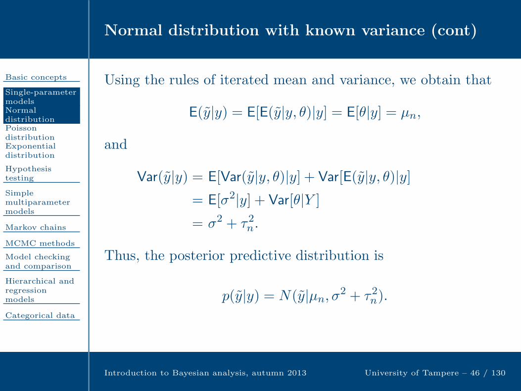
Thus, the posterior predictive distribution is
p(y|y) = N(y|µn, σ2 + τ2n).

Poisson distribution
Basic concepts
Single-parametermodelsNormaldistributionPoissondistributionExponentialdistribution
Hypothesistesting
Simplemultiparametermodels
Markov chains
MCMC methods
Model checkingand comparison
Hierarchical andregressionmodels
Categorical data
Introduction to Bayesian analysis, autumn 2013 University of Tampere – 47 / 130
The Poisson distribution is often used to model rare incidents,such as traffic accidents or rare diseases. For a vectory = (y1, ..., yn) of iid observation, the likelihood is
p(y|θ) =n∏
i=1
θyi
yi!e−θ ∝ θ
∑yie−nθ.
Given that the prior distribution is Gamma(α, β), the posterior
p(θ|y) ∝ p(θ)p(y|θ)∝ θα−1e−βθθ
∑yie−nθ
∝ θα+∑
yi−1e−(β+n)θ
is Gamma(α+∑yi, β + n).
Poisson distribution (cont)
Basic concepts
Single-parametermodelsNormaldistributionPoissondistributionExponentialdistribution
Hypothesistesting
Simplemultiparametermodels
Markov chains
MCMC methods
Model checkingand comparison
Hierarchical andregressionmodels
Categorical data
Introduction to Bayesian analysis, autumn 2013 University of Tampere – 48 / 130
The negative binomial distribution. When the prior andposterior distributions can be written in closed form, themarginal likelihood p(y) can be computed using the formula
p(y) =p(y|θ)p(θ)p(θ|y) .
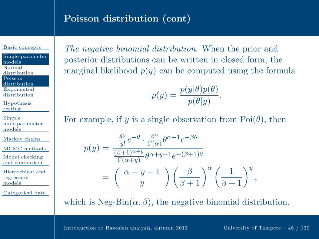
For example, if y is a single observation from Poi(θ), then
p(y) =
θy
y! e−θ · βα
Γ(α)θα−1e−βθ
(β+1)α+y
Γ(α+y) θα+y−1e−(β+1)θ
=
(α+ y − 1
y
)(β
β + 1
)α( 1
β + 1
)y
,
which is Neg-Bin(α, β), the negative binomial distribution.
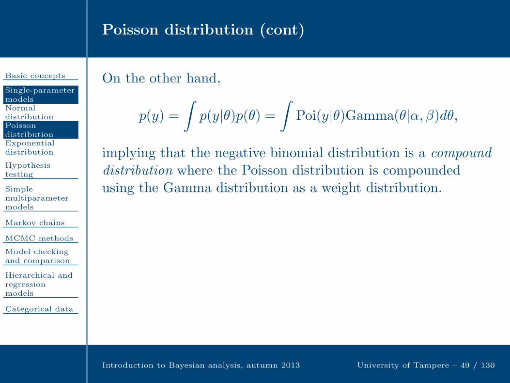
Poisson distribution (cont)
Basic concepts
Single-parametermodelsNormaldistributionPoissondistributionExponentialdistribution
Hypothesistesting
Simplemultiparametermodels
Markov chains
MCMC methods
Model checkingand comparison
Hierarchical andregressionmodels
Categorical data
Introduction to Bayesian analysis, autumn 2013 University of Tampere – 49 / 130
On the other hand,
p(y) =
∫p(y|θ)p(θ) =
∫Poi(y|θ)Gamma(θ|α, β)dθ,
implying that the negative binomial distribution is a compound
distribution where the Poisson distribution is compoundedusing the Gamma distribution as a weight distribution.
In many applications, the data are distributed as
yi ∼ Poi(xiθ),
where the xi are known values of an explanatory variable. Inepidemiology, xi is called exposure of the ith unit. With priordistribution Gamma(α, β), the posterior becomesGamma(α+
∑yi, β +
∑xi).
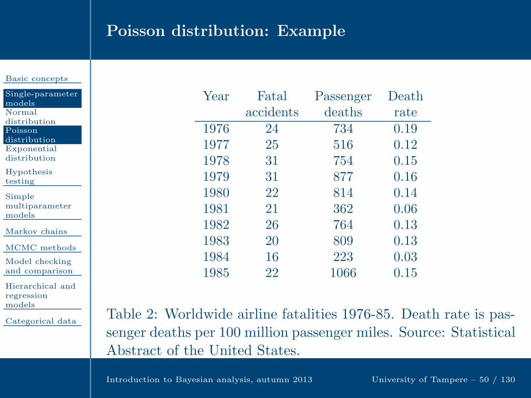
Poisson distribution: Example
Basic concepts
Single-parametermodelsNormaldistributionPoissondistributionExponentialdistribution
Hypothesistesting
Simplemultiparametermodels
Markov chains
MCMC methods
Model checkingand comparison
Hierarchical andregressionmodels
Categorical data
Introduction to Bayesian analysis, autumn 2013 University of Tampere – 50 / 130
Year Fatal Passenger Deathaccidents deaths rate
1976 24 734 0.191977 25 516 0.121978 31 754 0.151979 31 877 0.161980 22 814 0.141981 21 362 0.061982 26 764 0.131983 20 809 0.131984 16 223 0.031985 22 1066 0.15
Table 2: Worldwide airline fatalities 1976-85. Death rate is pas-senger deaths per 100 million passenger miles. Source: StatisticalAbstract of the United States.
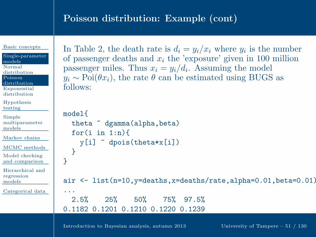
Poisson distribution: Example (cont)
Basic concepts
Single-parametermodelsNormaldistributionPoissondistributionExponentialdistribution
Hypothesistesting
Simplemultiparametermodels
Markov chains
MCMC methods
Model checkingand comparison
Hierarchical andregressionmodels
Categorical data
Introduction to Bayesian analysis, autumn 2013 University of Tampere – 51 / 130
In Table 2, the death rate is di = yi/xi where yi is the numberof passenger deaths and xi the ’exposure’ given in 100 millionpassenger miles. Thus xi = yi/di. Assuming the modelyi ∼ Poi(θxi), the rate θ can be estimated using BUGS asfollows:
model
theta ~ dgamma(alpha,beta)
for(i in 1:n)
y[i] ~ dpois(theta*x[i])
air <- list(n=10,y=deaths,x=deaths/rate,alpha=0.01,beta=0.01)
...
2.5% 25% 50% 75% 97.5%
0.1182 0.1201 0.1210 0.1220 0.1239
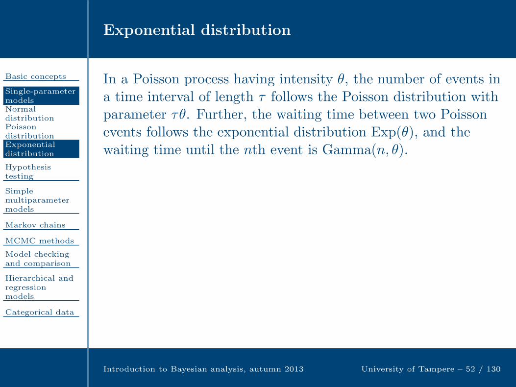
Exponential distribution
Basic concepts
Single-parametermodelsNormaldistributionPoissondistributionExponentialdistribution
Hypothesistesting
Simplemultiparametermodels
Markov chains
MCMC methods
Model checkingand comparison
Hierarchical andregressionmodels
Categorical data
Introduction to Bayesian analysis, autumn 2013 University of Tampere – 52 / 130
In a Poisson process having intensity θ, the number of events ina time interval of length τ follows the Poisson distribution withparameter τθ. Further, the waiting time between two Poissonevents follows the exponential distribution Exp(θ), and thewaiting time until the nth event is Gamma(n, θ).
The exponential distribution can also be used to model lifetimes of objects that do not wear out, since in this model theexpected remaining life time is independent of the time theobject has already survived.

Exponential distribution
Basic concepts
Single-parametermodelsNormaldistributionPoissondistributionExponentialdistribution
Hypothesistesting
Simplemultiparametermodels
Markov chains
MCMC methods
Model checkingand comparison
Hierarchical andregressionmodels
Categorical data
Introduction to Bayesian analysis, autumn 2013 University of Tampere – 52 / 130
In a Poisson process having intensity θ, the number of events ina time interval of length τ follows the Poisson distribution withparameter τθ. Further, the waiting time between two Poissonevents follows the exponential distribution Exp(θ), and thewaiting time until the nth event is Gamma(n, θ).
The exponential distribution can also be used to model lifetimes of objects that do not wear out, since in this model theexpected remaining life time is independent of the time theobject has already survived. If Y ∼ Exp(θ), then
Pr(Y ≤ y|Y > y0) =Pr(y0 < Y ≤ y)
Pr(Y > y0=
Pr(Y ≤ y)− Pr(Y ≤ y0)
Pr(Y > y0)
=(1− e−θy)− (1− e−θy0)
e−θy0
= 1− e−θ(y−y0),
which is the exponential distribution function starting at y0.

Exponential distribution (cont)
Basic concepts
Single-parametermodelsNormaldistributionPoissondistributionExponentialdistribution
Hypothesistesting
Simplemultiparametermodels
Markov chains
MCMC methods
Model checkingand comparison
Hierarchical andregressionmodels
Categorical data
Introduction to Bayesian analysis, autumn 2013 University of Tampere – 53 / 130
Bayesian analysis. Let y = (y1, ..., yn) be a random sample formExp(θ) and let Gamma(α, β) be the prior. Then the posterior is
p(θ|y) ∝ p(θ)p(y|θ) ∝ θα−1e−βθn∏
i=1
θe−θyi
∝ θα+n−1e−θ(β+∑
yi),
which is Gamma(α+ n, β +∑yi) distribution.
Censored observations. Assume that the observations y1, ...ymare known to be larger than U , while the exact values ofym+1, ..., yn are known. Then the values y1, ...ym are calledright-censored. On the other hand, if some observations areknown to be less or equal to some threshold L, they are calledleft-censored.

Exponential distribution (cont)
Basic concepts
Single-parametermodelsNormaldistributionPoissondistributionExponentialdistribution
Hypothesistesting
Simplemultiparametermodels
Markov chains
MCMC methods
Model checkingand comparison
Hierarchical andregressionmodels
Categorical data
Introduction to Bayesian analysis, autumn 2013 University of Tampere – 54 / 130
In the exponential case of right-censoring, the likelihood is
p(y|θ) =m∏
i=1
Pr(Yi > U |θ)n∏
i=m+1
p(yi|θ)
=
m∏
i=1
e−θUn∏
i=m+1
θe−θyi = θn−me−θ(mU+∑
yi).
Thus, with prior Gamma(α, β), the posterior isGamma(α+ n−m,β +mU +
∑yi).
In the case of left-censoring, the likelihood is
p(y|θ) = (1− e−θL)m θn−me−θ∑
yi ,
so that the posterior distribution is nonstandard.
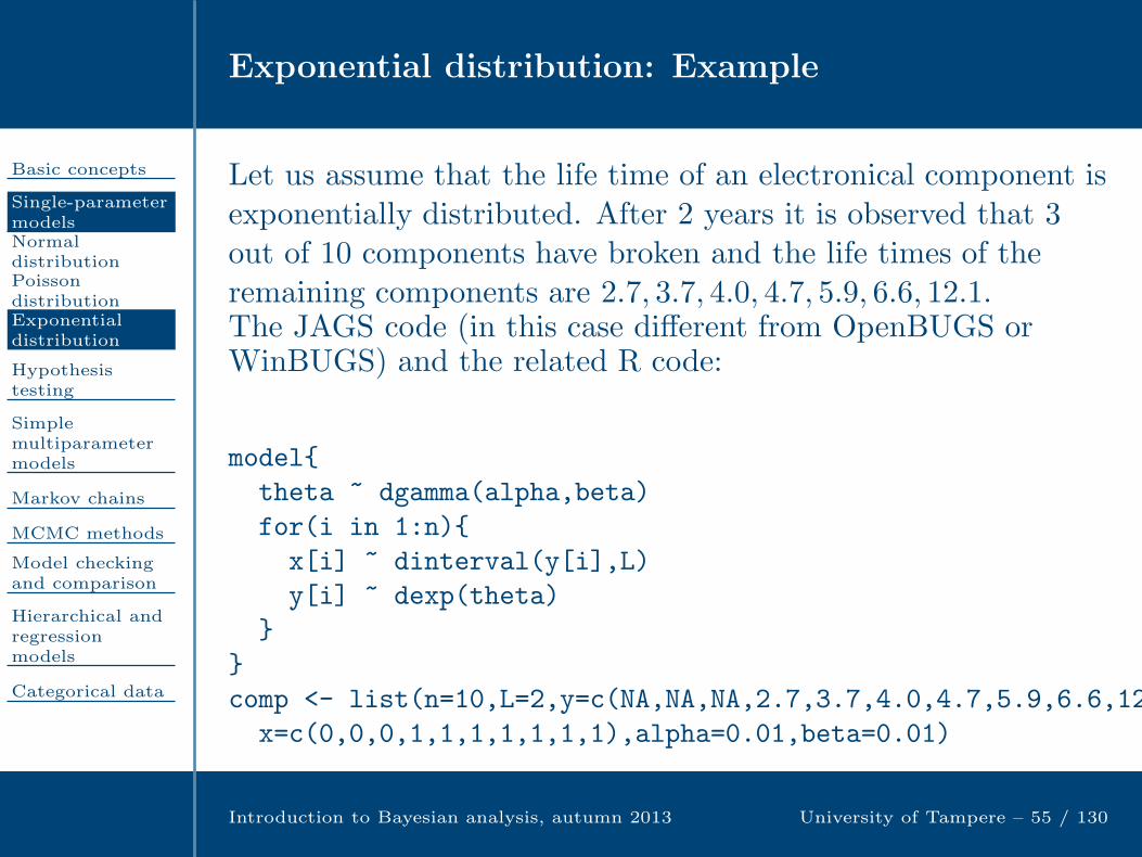
Exponential distribution: Example
Basic concepts
Single-parametermodelsNormaldistributionPoissondistributionExponentialdistribution
Hypothesistesting
Simplemultiparametermodels
Markov chains
MCMC methods
Model checkingand comparison
Hierarchical andregressionmodels
Categorical data
Introduction to Bayesian analysis, autumn 2013 University of Tampere – 55 / 130
Let us assume that the life time of an electronical component isexponentially distributed. After 2 years it is observed that 3out of 10 components have broken and the life times of theremaining components are 2.7, 3.7, 4.0, 4.7, 5.9, 6.6, 12.1.The JAGS code (in this case different from OpenBUGS orWinBUGS) and the related R code:
model
theta ~ dgamma(alpha,beta)
for(i in 1:n)
x[i] ~ dinterval(y[i],L)
y[i] ~ dexp(theta)
comp <- list(n=10,L=2,y=c(NA,NA,NA,2.7,3.7,4.0,4.7,5.9,6.6,12.1),
x=c(0,0,0,1,1,1,1,1,1,1),alpha=0.01,beta=0.01)

Hypothesis testing
Basic concepts
Single-parametermodels
Hypothesistesting
Definition
Example
Computation
Simplemultiparametermodels
Markov chains
MCMC methods
Model checkingand comparison
Hierarchical andregressionmodels
Categorical data
Introduction to Bayesian analysis, autumn 2013 University of Tampere – 56 / 130

Bayesian hypothesis testing
Basic concepts
Single-parametermodels
Hypothesistesting
Definition
Example
Computation
Simplemultiparametermodels
Markov chains
MCMC methods
Model checkingand comparison
Hierarchical andregressionmodels
Categorical data
Introduction to Bayesian analysis, autumn 2013 University of Tampere – 57 / 130
The frequentist approach to hypothesis testing would comparea null hypothesis H0 with an alternative H1 through a teststatistic T which typically obtains a larger value when H1 istrue than when H0 is true. The null hypothesis is rejected witha level α if the observed value of the test statistic, tobs, is largerthan the critical value tC where Pr(T > tC |H0) = α. Theso-called p-value, p = Pr(T ≥ tobs|H0), is a related concept.
In frequentist statistics, we do not assign probabilities tohypotheses. In particular, the p-value cannot be interpreted asp(H0). On the contrary, in the Bayesian approach, we mayassign the prior probabilities p(H0) and p(H1), and, usingBayes’ theorem, compute the posterior probabilities
p(Hi|y) =p(Hi)p(y|Hi)
p(H0)p(y|H0) + p(H1)p(y|H1), i = 0, 1.

Bayesian hypothesis testing (cont)
Basic concepts
Single-parametermodels
Hypothesistesting
Definition
Example
Computation
Simplemultiparametermodels
Markov chains
MCMC methods
Model checkingand comparison
Hierarchical andregressionmodels
Categorical data
Introduction to Bayesian analysis, autumn 2013 University of Tampere – 58 / 130
In the frequentist approach it is not absolutely necessary tospecify an alternative hypothesis. Further, if an alternative isspecified, the p-value is independent of it. In the Bayesianapproach, the both hypotheses must be fully specified.
One usually computes the posterior odds
p(H1|yp(H0|y)
=p(y|H1)
p(y|H0)× p(H1)
p(H0),
which depends on the data y only through the Bayes factor
B10 = p(y|H1)/p(y|H0).
In the case that a hypothesis is composite (not simple), theunknown parameters should be first integrated out:
p(y|Hi) =
∫p(y|θi, Hi)p(θi|Hi)dθi, i = 0, 1.
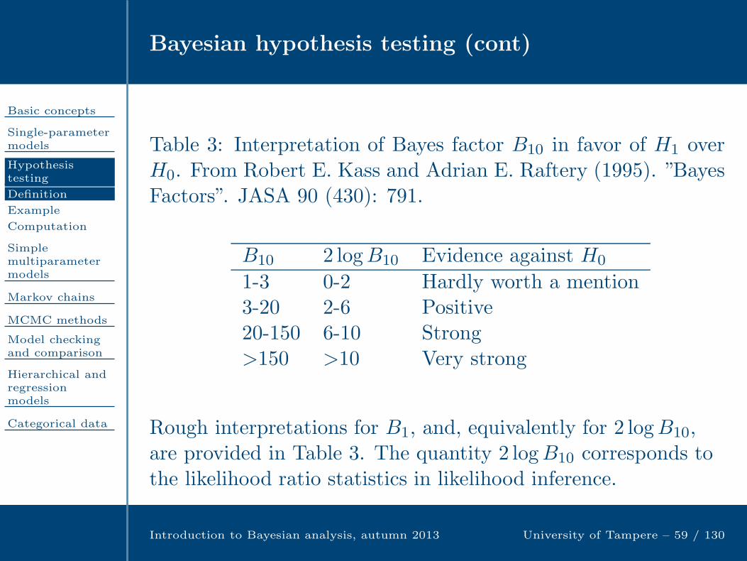
Bayesian hypothesis testing (cont)
Basic concepts
Single-parametermodels
Hypothesistesting
Definition
Example
Computation
Simplemultiparametermodels
Markov chains
MCMC methods
Model checkingand comparison
Hierarchical andregressionmodels
Categorical data
Introduction to Bayesian analysis, autumn 2013 University of Tampere – 59 / 130
Table 3: Interpretation of Bayes factor B10 in favor of H1 overH0. From Robert E. Kass and Adrian E. Raftery (1995). ”BayesFactors”. JASA 90 (430): 791.
B10 2 logB10 Evidence against H0
1-3 0-2 Hardly worth a mention3-20 2-6 Positive20-150 6-10 Strong>150 >10 Very strong
Rough interpretations for B1, and, equivalently for 2 logB10,are provided in Table 3. The quantity 2 logB10 corresponds tothe likelihood ratio statistics in likelihood inference.

Bayesian hypothesis testing: Example
Basic concepts
Single-parametermodels
Hypothesistesting
Definition
Example
Computation
Simplemultiparametermodels
Markov chains
MCMC methods
Model checkingand comparison
Hierarchical andregressionmodels
Categorical data
Introduction to Bayesian analysis, autumn 2013 University of Tampere – 60 / 130
Table 4: The log Bayes factors 2 logBτ0 for HUS data.
1970 1971 1972 1973 1974 1975 1976
y 1 5 3 2 2 1 0α = β = 1 4.9 -0.5 0.6 3.9 7.5 13 24α = β = 0.01 -1.3 -5.9 -4.5 -1.0 3.0 9.7 20α = β = 0.0001 -10 -15 -14 -10 -6.1 0.6 11
1977 1978 1979 1980 1981 1982 1983
y 0 2 1 1 7 11 4α = β = 1 35 41 51 63 55 38 42α = β = 0.01 32 39 51 64 57 40 47α = β = 0.0001 23 30 42 55 48 31 38
1984 1985 1986 1987 1988 1989
y 7 10 16 16 9 15α = β = 1 40 31 11 -2.9 -5.3 0α = β = 0.01 46 38 18 1.8 1.2 0α = β = 0.0001 37 29 8.8 -7.1 -7.7 0
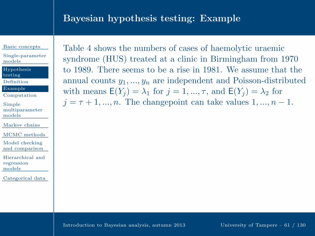
Bayesian hypothesis testing: Example
Basic concepts
Single-parametermodels
Hypothesistesting
Definition
Example
Computation
Simplemultiparametermodels
Markov chains
MCMC methods
Model checkingand comparison
Hierarchical andregressionmodels
Categorical data
Introduction to Bayesian analysis, autumn 2013 University of Tampere – 61 / 130
Table 4 shows the numbers of cases of haemolytic uraemicsyndrome (HUS) treated at a clinic in Birmingham from 1970to 1989. There seems to be a rise in 1981. We assume that theannual counts y1, ..., yn are independent and Poisson-distributedwith means E(Yj) = λ1 for j = 1, ..., τ , and E(Yj) = λ2 forj = τ + 1, ..., n. The changepoint can take values 1, ..., n− 1.
Our baseline model H0 is that there is no change, λ1 = λ2 = λ,and the alternative Hτ that there is a change after τ years.Under Hτ we assume that λ1 and λ2 have independent priorswith parameters α and β. Then p(y|Hτ ) equals
∫∞
0
τ∏
j=1
λyj
1
yj !e−λ1 ·β
αλα−11 e−βλ1
Γ(α)dλ1
∫∞
0
n∏
j=τ+1
λyj
1
yj !e−λ2 ·β
αλα−12 e−βλ2
Γ(α)dλ2,

Bayesian hypothesis testing: Example
Basic concepts
Single-parametermodels
Hypothesistesting
Definition
Example
Computation
Simplemultiparametermodels
Markov chains
MCMC methods
Model checkingand comparison
Hierarchical andregressionmodels
Categorical data
Introduction to Bayesian analysis, autumn 2013 University of Tampere – 62 / 130
which can be simplified as
β2α
Γ(α)2∏n
j=1 yj !
Γ(α+ sτ )Γ(α+ sn − sτ )
(β + τ)α+sτ (β + n− τ)α+sn−sτ,
where sτ = y1 + ...+ yτ and sn = y1 + ...+ yn.
Under H0 we also assume that λ ∼ Gamma(α, β). Then theBayes factor for a changepoint in year τ is
Bτ0 =Γ(α+ sτ )Γ(α+ sn − sτ )β
α(β + n)α+sn
Γ(α)Γ(α+ sn)(β + τ)α+sτ (β + n− τ)α+sn−sτ, τ = 1, ..., n
From Table 4 we see that there is a very strong evidence forchange in 1976–1985 for all priors.

Computing marginal likelihoods
Basic concepts
Single-parametermodels
Hypothesistesting
Definition
Example
Computation
Simplemultiparametermodels
Markov chains
MCMC methods
Model checkingand comparison
Hierarchical andregressionmodels
Categorical data
Introduction to Bayesian analysis, autumn 2013 University of Tampere – 63 / 130
Bayes factors can be presented in closed form only in simpleconjugate situations, but various simulation-based methodshave been suggested. One simple example is the harmonic
mean method, which is based on the result
1
T
T∑
t=1
1
p(y|θ(t))p−→ 1
p(y)as T → ∞,
where θ(t), t = 1, ..., T are independent simulations from p(θ|y).The result follows from the law of large numbers.
This estimator is somewhat unstable, since occasional values ofθ(t) with small likelihood have a large effect on it. Therefore,several modifications of the method have been developed. Moreadvanced methods, such as path sampling, are effective, butusually require problem-specific tuning.

Model choice: Example (cont)
Basic concepts
Single-parametermodels
Hypothesistesting
Definition
Example
Computation
Simplemultiparametermodels
Markov chains
MCMC methods
Model checkingand comparison
Hierarchical andregressionmodels
Categorical data
Introduction to Bayesian analysis, autumn 2013 University of Tampere – 64 / 130
Another approach is to consider the model choice as a discreteparameter. This is generally a more reliable method to obtainposterior model probabilities with BUGS (BUGS book, 2013).
In the following, we present a code to estimate the modelprobabilities in the HUS example. We give an equal priorprobability, 1/n, to each of the models Hτ , τ = 1, ..., n. Here,Hn corresponds to H0.
Figure 3 shows the posterior model probabilities. The values 11and 12 are the most probable change points:Pr(τ = 11|y) ≈ 0.97 and Pr(τ = 12|y) ≈ 0.03.
Model choice: Example (cont)
Basic concepts
Single-parametermodels
Hypothesistesting
Definition
Example
Computation
Simplemultiparametermodels
Markov chains
MCMC methods
Model checkingand comparison
Hierarchical andregressionmodels
Categorical data
Introduction to Bayesian analysis, autumn 2013 University of Tampere – 65 / 130
model
for(i in 1:n)
q[i] <- 1/n
tau ~ dcat(q[])
for(i in 1:2)
lambda[i] ~ dgamma(alpha,beta)
for(i in 1:n)
mu[i] <- lambda[1]+
step(i-tau-0.1)*(lambda[2]-lambda[1])
y[i] ~ dpois(mu[i])
HUS <- list(n=20, y= c(1,5,3,2,2,1,0,0,2,1,1,7,11,4,7,10,16,16,9,15),
alpha=0.01,beta=0.01)
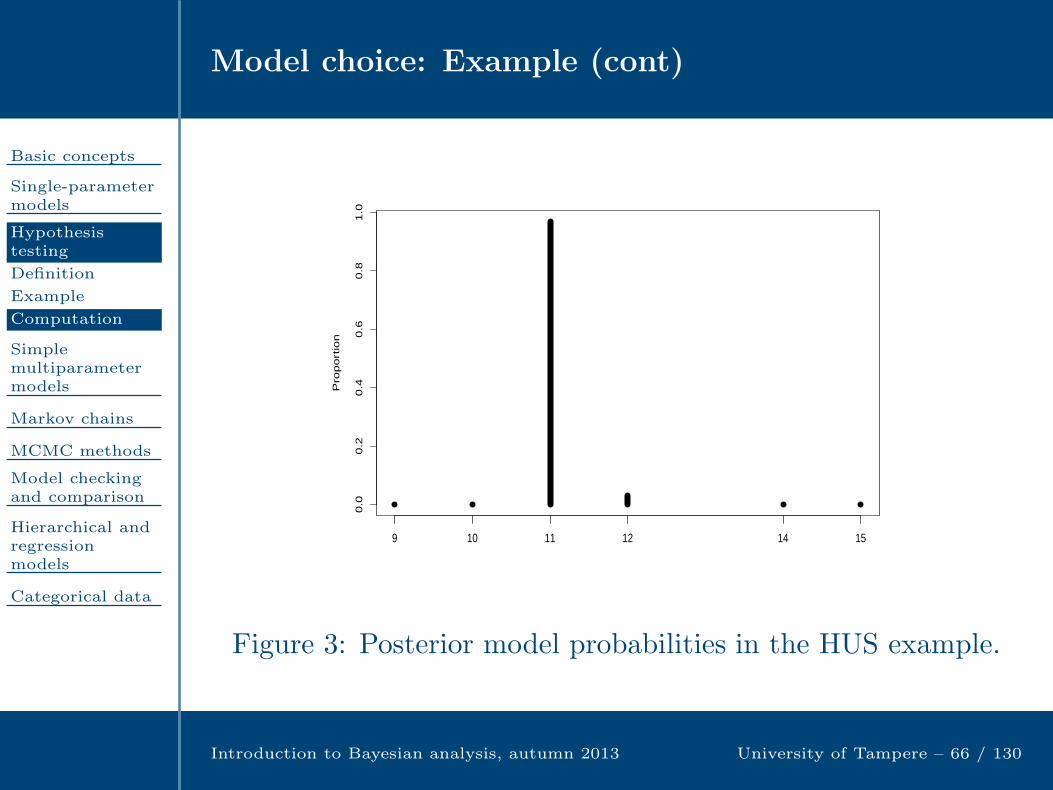
Model choice: Example (cont)
Basic concepts
Single-parametermodels
Hypothesistesting
Definition
Example
Computation
Simplemultiparametermodels
Markov chains
MCMC methods
Model checkingand comparison
Hierarchical andregressionmodels
Categorical data
Introduction to Bayesian analysis, autumn 2013 University of Tampere – 66 / 130
0.0
0.2
0.4
0.6
0.8
1.0
Pro
po
rtio
n
9 10 11 12 14 15
Figure 3: Posterior model probabilities in the HUS example.
Simple multiparameter models
Basic concepts
Single-parametermodels
Hypothesistesting
SimplemultiparametermodelsNormaldistribution
Example
Multinomialdistribution
Example
Markov chains
MCMC methods
Model checkingand comparison
Hierarchical andregressionmodels
Categorical data
Introduction to Bayesian analysis, autumn 2013 University of Tampere – 67 / 130

Normal distribution with unknown mean andvariance
Basic concepts
Single-parametermodels
Hypothesistesting
SimplemultiparametermodelsNormaldistribution
Example
Multinomialdistribution
Example
Markov chains
MCMC methods
Model checkingand comparison
Hierarchical andregressionmodels
Categorical data
Introduction to Bayesian analysis, autumn 2013 University of Tampere – 68 / 130
Next we consider simple models having more than oneparameter. Let us assume that y = (y1, ..., yn) is a randomsample from N(µ, σ2) where both µ and σ2 are unknown. If thejoint prior is p(µ, σ2) ∝ 1/σ2, or equivalently p(µ, log(σ2)) ∝ 1,the posterior is
p(µ, σ2|y) ∝ 1
σ2× 1
(σ2)n/2exp
(− 1
2σ2
n∑
i=1
(yi − µ)2
)
=1
(σ2)n/2+1exp
(− 1
2σ2
[n∑
i=1
(yi − y)2 + n(y − µ)2
])
=1
(σ2)n/2+1exp
(− 1
2σ2[(n− 1)s2 + n(y − µ)2]
),
where s2 = 1n−1
∑ni=1(yi − y)2 is the sample variance.
Normal distribution (cont)
Basic concepts
Single-parametermodels
Hypothesistesting
SimplemultiparametermodelsNormaldistribution
Example
Multinomialdistribution
Example
Markov chains
MCMC methods
Model checkingand comparison
Hierarchical andregressionmodels
Categorical data
Introduction to Bayesian analysis, autumn 2013 University of Tampere – 69 / 130
The marginal posterior of σ2 is obtained by integrating µ out:
p(σ2|y) ∝∫ ∞
−∞
1
(σ2)n/2+1exp
(− 1
2σ2[(n− 1)s2 + n(y − µ)2]
)dµ.
The integral of the factor exp(− 1
2σ2n(y − µ)2)is a simple
normal integral, so
p(σ2|y) ∝ 1
(σ2)n/2+1exp
(− 1
2σ2(n− 1)s2
)√2πσ2/n
∝ 1
(σ2)(n+1)/2exp
(−(n− 1)s2
2σ2
).
This is a scaled inverse-χ2-density:
σ2|y ∼ Inv-χ2(n− 1, s2).

Normal distribution (cont)
Basic concepts
Single-parametermodels
Hypothesistesting
SimplemultiparametermodelsNormaldistribution
Example
Multinomialdistribution
Example
Markov chains
MCMC methods
Model checkingand comparison
Hierarchical andregressionmodels
Categorical data
Introduction to Bayesian analysis, autumn 2013 University of Tampere – 70 / 130
Thus, (n− 1)s2/σ2 | y ∼ χ2n−1. This is analogous with the
corresponding sampling theory result. However, in samplingtheory, s2 is considered random, while here σ2 is random.
By making the substitution
z =A
σ2, where A = (n− 1)s2 + n(y − µ)2,
we obtain the marginal density of µ:
p(µ|y) ∝∫
∞
0
1
(σ2)n/2+1exp
(− 1
2σ2[(n− 1)s2 + n(y − µ)2]
)dσ2
∝ A−n/2
∫∞
0
zn/2−1 exp(−z)dz
∝[1 +
n(µ− y)2
(n− 1)s2
]−n/2
.

Normal distribution: Speed of light (example)
Basic concepts
Single-parametermodels
Hypothesistesting
SimplemultiparametermodelsNormaldistribution
Example
Multinomialdistribution
Example
Markov chains
MCMC methods
Model checkingand comparison
Hierarchical andregressionmodels
Categorical data
Introduction to Bayesian analysis, autumn 2013 University of Tampere – 71 / 130
This is the tn−1(y, s2/n) density. Thus, (µ− y)/(s/
√n) | y
∼ tn−1. This is again analogous to the sampling theory result.It can also be shown (exercise) that the density of a newobservation y is tn−1(y, s
2(1 + 1/n)). The posterior can besimulated using p(σ2|y) and p(µ|σ2, y) = N(µ|y, σ2/n).
Normal distribution: Speed of light (example)
Basic concepts
Single-parametermodels
Hypothesistesting
SimplemultiparametermodelsNormaldistribution
Example
Multinomialdistribution
Example
Markov chains
MCMC methods
Model checkingand comparison
Hierarchical andregressionmodels
Categorical data
Introduction to Bayesian analysis, autumn 2013 University of Tampere – 71 / 130
This is the tn−1(y, s2/n) density. Thus, (µ− y)/(s/
√n) | y
∼ tn−1. This is again analogous to the sampling theory result.It can also be shown (exercise) that the density of a newobservation y is tn−1(y, s
2(1 + 1/n)). The posterior can besimulated using p(σ2|y) and p(µ|σ2, y) = N(µ|y, σ2/n).Example. Estimating the speed of light. Simon Newcomb madean experiment in 1882 to measure the speed of light. Hemeasured the time light travels 7442 meters. Figure 4 showsthat there are two outliers, so the normal distribution as such isnot a very good model. However, for the sake of illustration, weassume that the observations are independent and fromN(µ, σ2). With the noninformative prior p(µ, σ2) ∝ 1/σ2, the95% posterior interval is (y ± t(n−1);0.025s/
√n) = (23.6, 28.9)
where n = 66, y = 26.2 and s = 10.8. Further, the predictioninterval is (y ± t(n−1);0.025s
√1 + 1/n) = (4.6, 47.8).
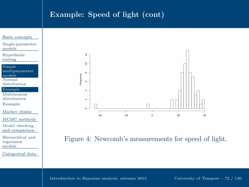
Example: Speed of light (cont)
Basic concepts
Single-parametermodels
Hypothesistesting
SimplemultiparametermodelsNormaldistribution
Example
Multinomialdistribution
Example
Markov chains
MCMC methods
Model checkingand comparison
Hierarchical andregressionmodels
Categorical data
Introduction to Bayesian analysis, autumn 2013 University of Tampere – 72 / 130
Fre
qu
en
cy
−40 −20 0 20 40
02
46
81
01
2
Figure 4: Newcomb’s measurements for speed of light.

Multinomial distribution
Basic concepts
Single-parametermodels
Hypothesistesting
SimplemultiparametermodelsNormaldistribution
Example
Multinomialdistribution
Example
Markov chains
MCMC methods
Model checkingand comparison
Hierarchical andregressionmodels
Categorical data
Introduction to Bayesian analysis, autumn 2013 University of Tampere – 73 / 130
If y = (y1, ...yk) is multinomially distributed with parameters nand θ = (θ1, ..., θk) (denoted as Multin(n; θ)) then the likelihoodis
p(θ|y) ∝ θy11 θy22 ...θ
ykk
where θi ≥ 0 for all i = 1, ..., k and∑k
i=1 θi = 1.
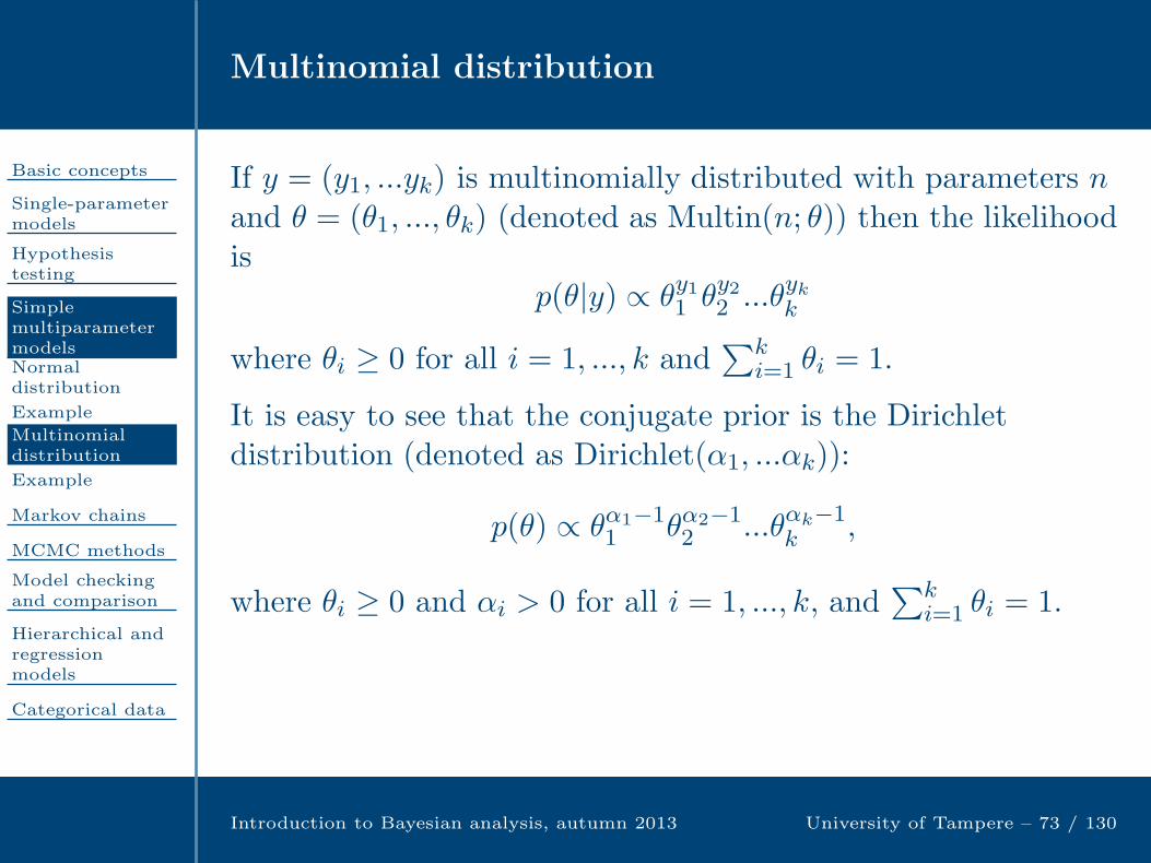
It is easy to see that the conjugate prior is the Dirichletdistribution (denoted as Dirichlet(α1, ...αk)):
p(θ) ∝ θα1−11 θα2−1
2 ...θαk−1k ,
where θi ≥ 0 and αi > 0 for all i = 1, ..., k, and∑k
i=1 θi = 1.
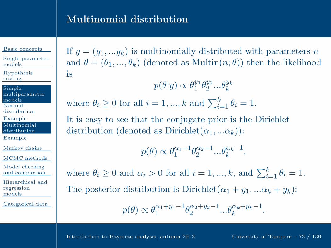
The posterior distribution is Dirichlet(α1 + y1, ...αk + yk):
p(θ) ∝ θα1+y1−11 θα2+y2−1
2 ...θαk+yk−1k .

Multinomial distribution: Presidential elections(example)
Basic concepts
Single-parametermodels
Hypothesistesting
SimplemultiparametermodelsNormaldistribution
Example
Multinomialdistribution
Example
Markov chains
MCMC methods
Model checkingand comparison
Hierarchical andregressionmodels
Categorical data
Introduction to Bayesian analysis, autumn 2013 University of Tampere – 74 / 130
In January 2006, Taloustutkimus (Economic Survey in Finland)interviewed 1582 adults about their preferences in theforthcoming presidential election. Out of those who expressedtheir opinion, 52% supported Halonen, 20% Niinisto, 18%Vanhanen, and 10% other candidates. The proportion ofuncertain respondents was 29%.
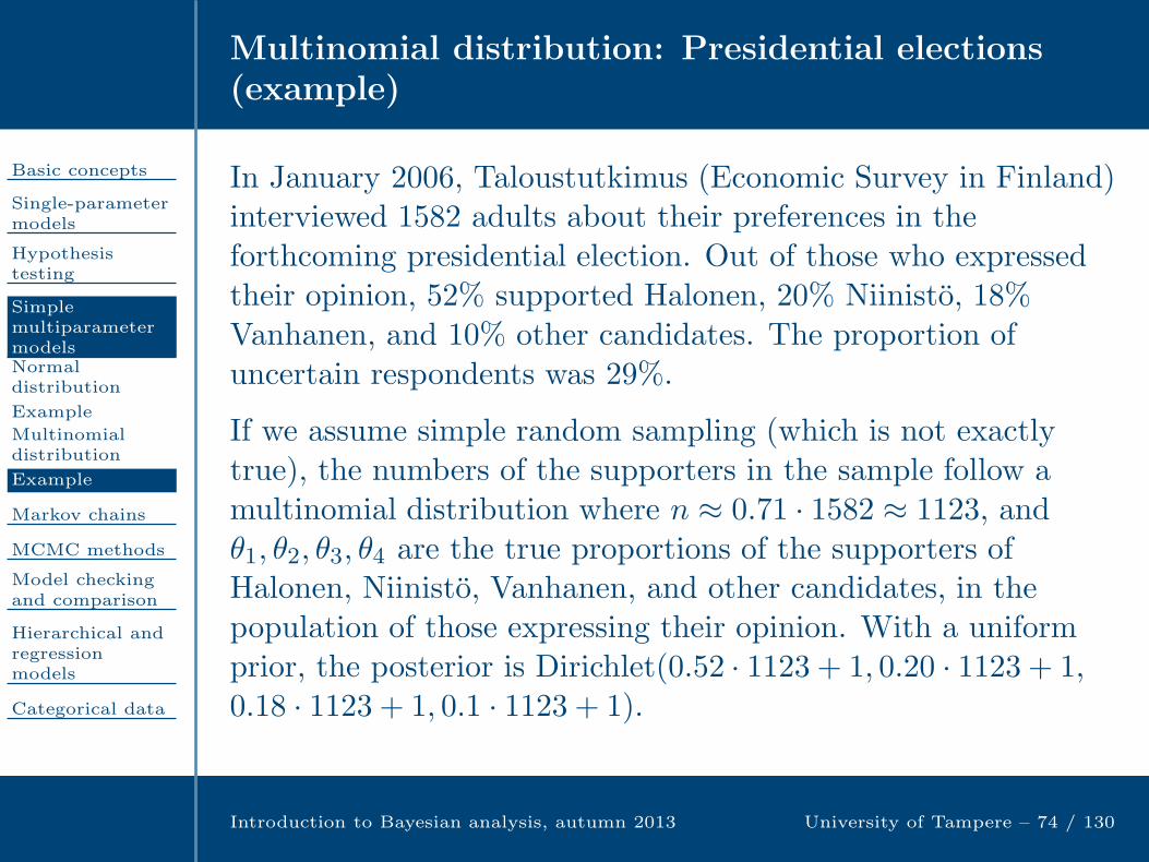
If we assume simple random sampling (which is not exactlytrue), the numbers of the supporters in the sample follow amultinomial distribution where n ≈ 0.71 · 1582 ≈ 1123, andθ1, θ2, θ3, θ4 are the true proportions of the supporters ofHalonen, Niinisto, Vanhanen, and other candidates, in thepopulation of those expressing their opinion. With a uniformprior, the posterior is Dirichlet(0.52 · 1123 + 1, 0.20 · 1123 + 1,0.18 · 1123 + 1, 0.1 · 1123 + 1).
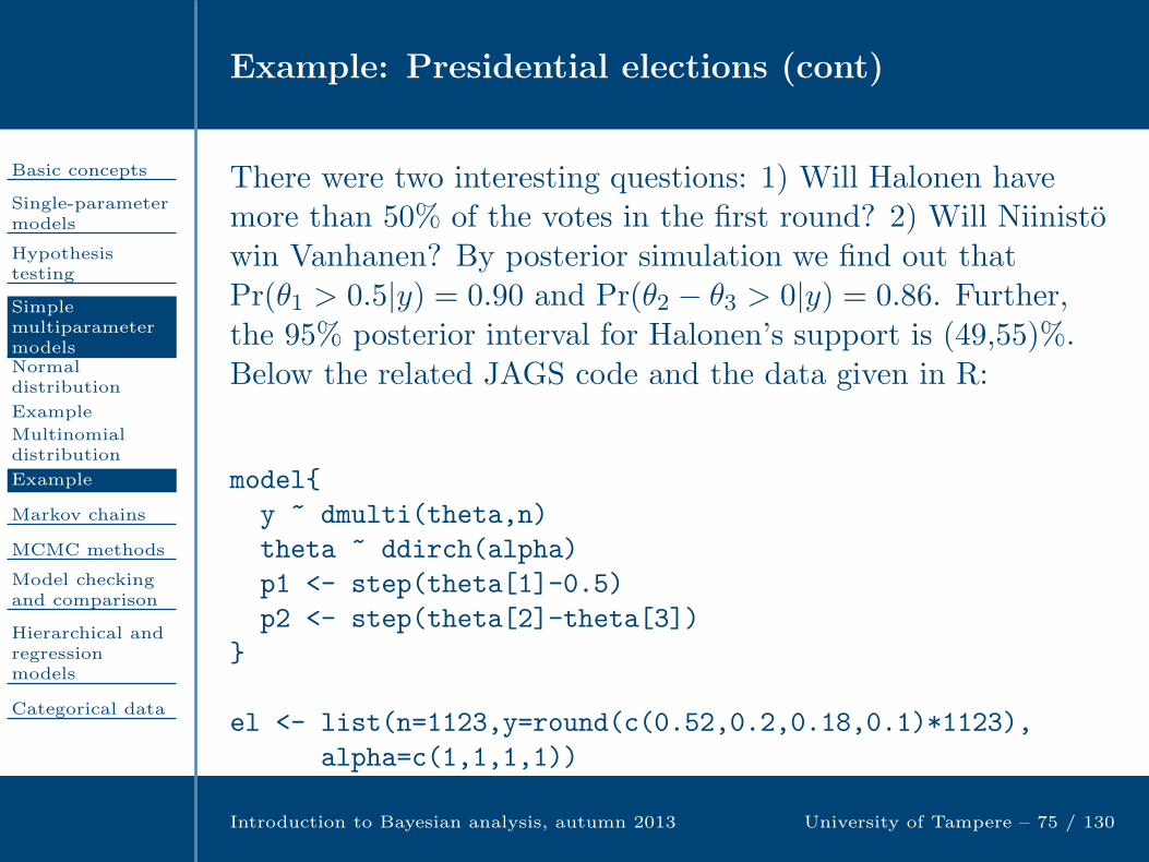
Example: Presidential elections (cont)
Basic concepts
Single-parametermodels
Hypothesistesting
SimplemultiparametermodelsNormaldistribution
Example
Multinomialdistribution
Example
Markov chains
MCMC methods
Model checkingand comparison
Hierarchical andregressionmodels
Categorical data
Introduction to Bayesian analysis, autumn 2013 University of Tampere – 75 / 130
There were two interesting questions: 1) Will Halonen havemore than 50% of the votes in the first round? 2) Will Niinistowin Vanhanen? By posterior simulation we find out thatPr(θ1 > 0.5|y) = 0.90 and Pr(θ2 − θ3 > 0|y) = 0.86. Further,the 95% posterior interval for Halonen’s support is (49,55)%.Below the related JAGS code and the data given in R:
model
y ~ dmulti(theta,n)
theta ~ ddirch(alpha)
p1 <- step(theta[1]-0.5)
p2 <- step(theta[2]-theta[3])
el <- list(n=1123,y=round(c(0.52,0.2,0.18,0.1)*1123),
alpha=c(1,1,1,1))

Markov chains
Basic concepts
Single-parametermodels
Hypothesistesting
Simplemultiparametermodels
Markov chains
Estimation
Example
MCMC methods
Model checkingand comparison
Hierarchical andregressionmodels
Categorical data
Introduction to Bayesian analysis, autumn 2013 University of Tampere – 76 / 130

Estimation of Markov Chains
Basic concepts
Single-parametermodels
Hypothesistesting
Simplemultiparametermodels
Markov chains
Estimation
Example
MCMC methods
Model checkingand comparison
Hierarchical andregressionmodels
Categorical data
Introduction to Bayesian analysis, autumn 2013 University of Tampere – 77 / 130
Assume that we have observations y0, ..., yT from a timehomogenous Markov chain measured at time pointst = 0, 1, 2, ..., T . Then the likelihood can be written as
Pr(Y0 = y0, ..., YT = yT )
= Pr(Y0 = y0
T∏
t=1
Pr(Yt = yt|Yt−1 = yt−1)
= Pr(Y0 = y0)T∏
t=1
pyt−1,yt
= Pr(Y0 = y0)S∏
r=1
S∏
r=1
pnrsrs ,
where nrs denotes the number of transitions from r to s.
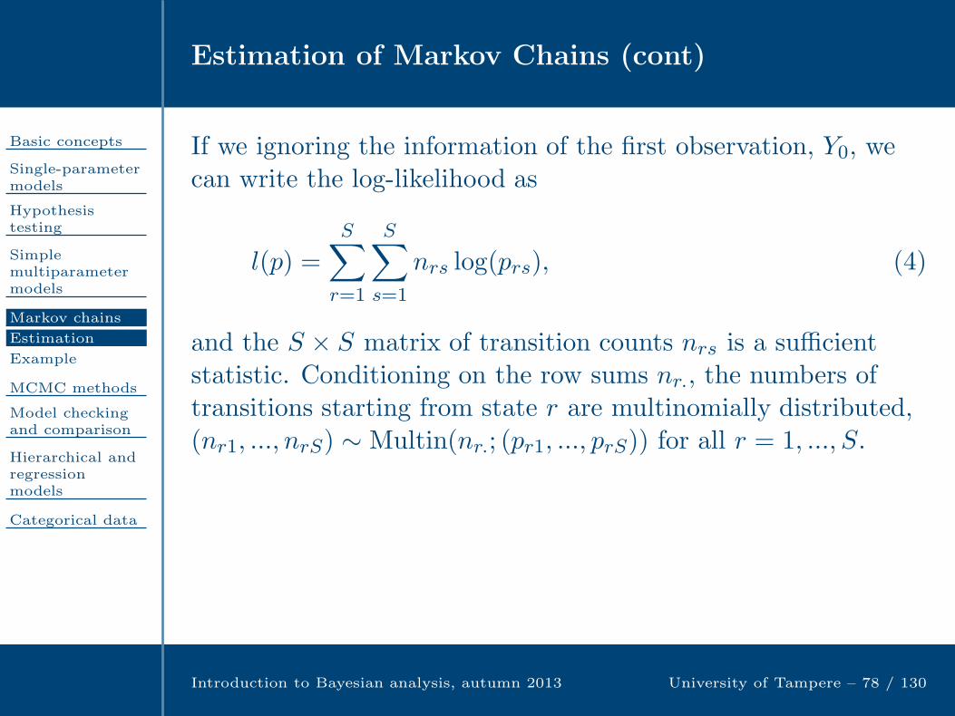
Estimation of Markov Chains (cont)
Basic concepts
Single-parametermodels
Hypothesistesting
Simplemultiparametermodels
Markov chains
Estimation
Example
MCMC methods
Model checkingand comparison
Hierarchical andregressionmodels
Categorical data
Introduction to Bayesian analysis, autumn 2013 University of Tampere – 78 / 130
If we ignoring the information of the first observation, Y0, wecan write the log-likelihood as
l(p) =S∑
r=1
S∑
s=1
nrs log(prs), (4)
and the S × S matrix of transition counts nrs is a sufficientstatistic. Conditioning on the row sums nr., the numbers oftransitions starting from state r are multinomially distributed,(nr1, ..., nrS) ∼ Multin(nr.; (pr1, ..., prS)) for all r = 1, ..., S.
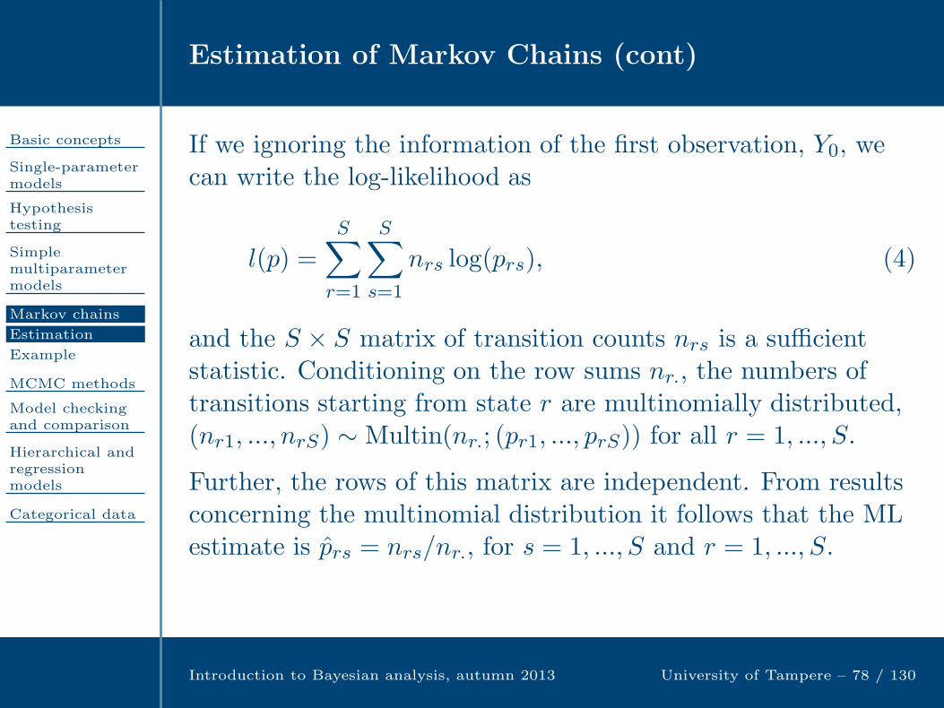
Further, the rows of this matrix are independent. From resultsconcerning the multinomial distribution it follows that the MLestimate is prs = nrs/nr., for s = 1, ..., S and r = 1, ..., S.
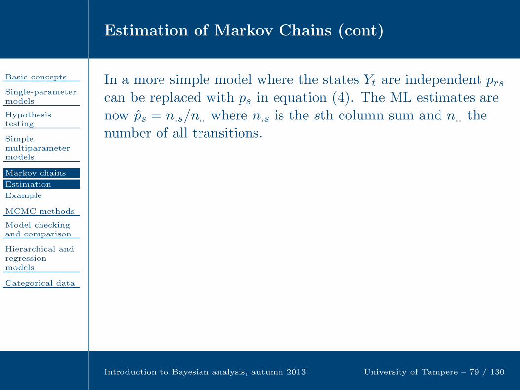
Estimation of Markov Chains (cont)
Basic concepts
Single-parametermodels
Hypothesistesting
Simplemultiparametermodels
Markov chains
Estimation
Example
MCMC methods
Model checkingand comparison
Hierarchical andregressionmodels
Categorical data
Introduction to Bayesian analysis, autumn 2013 University of Tampere – 79 / 130
In a more simple model where the states Yt are independent prscan be replaced with ps in equation (4). The ML estimates arenow ps = n.s/n.. where n.s is the sth column sum and n.. thenumber of all transitions.
The likelihood ratio statistics for testing the independencehypothesis is given by
W = 2∑
r,s
nrs log
(prsps
)= 2
∑
r,s
nrs log
(nrsn..
nr·n·s
).
Under independence, there are S − 1 free parameters, while inthe general case, S(S − 1) parameters. Thus, underindependence, the test statistic is approximately χ2-distributedwith S(S − 1)− (S − 1) = (S − 1)2 degrees of freedom. Wapproximately equals the Pearson statistic for independence.
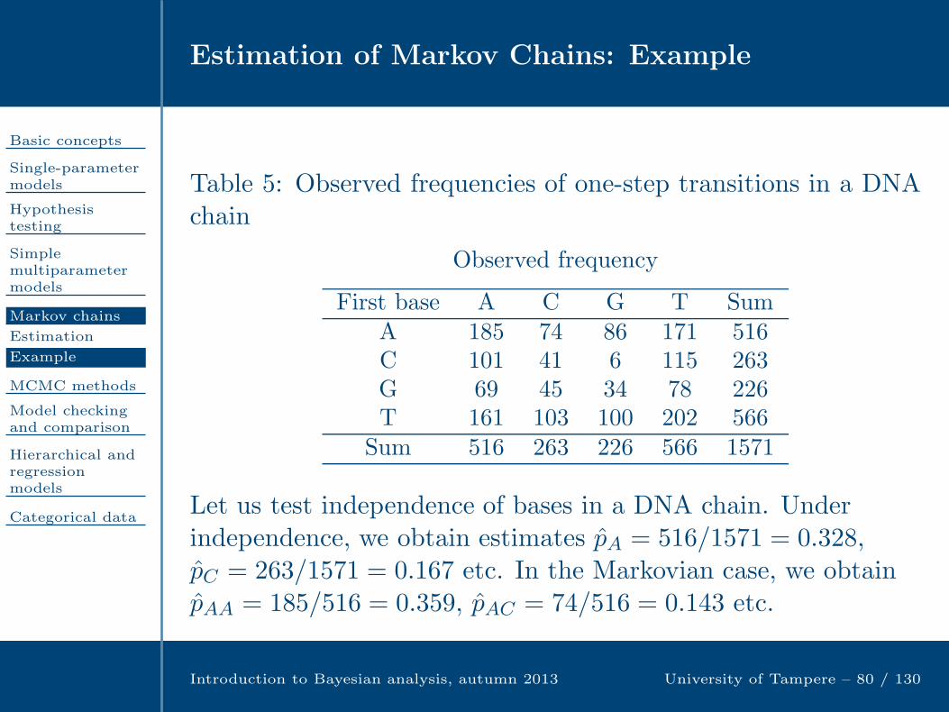
Estimation of Markov Chains: Example
Basic concepts
Single-parametermodels
Hypothesistesting
Simplemultiparametermodels
Markov chains
Estimation
Example
MCMC methods
Model checkingand comparison
Hierarchical andregressionmodels
Categorical data
Introduction to Bayesian analysis, autumn 2013 University of Tampere – 80 / 130
Table 5: Observed frequencies of one-step transitions in a DNAchain
Observed frequency
First base A C G T SumA 185 74 86 171 516C 101 41 6 115 263G 69 45 34 78 226T 161 103 100 202 566
Sum 516 263 226 566 1571
Let us test independence of bases in a DNA chain. Underindependence, we obtain estimates pA = 516/1571 = 0.328,pC = 263/1571 = 0.167 etc. In the Markovian case, we obtainpAA = 185/516 = 0.359, pAC = 74/516 = 0.143 etc.

Estimation of Markov Chains: Example (cont)
Basic concepts
Single-parametermodels
Hypothesistesting
Simplemultiparametermodels
Markov chains
Estimation
Example
MCMC methods
Model checkingand comparison
Hierarchical andregressionmodels
Categorical data
Introduction to Bayesian analysis, autumn 2013 University of Tampere – 81 / 130
If the independence hypothesis was correct, the test statistics Pand W would have approximate χ2
9-distributions. Now theirobserved values are 64.45 and 50.3 which make this hypothesishighly implausible.
The fit of the independence assumption can also be studiedgraphically. If this assumption was correct, the normalized
deviations Zrs = (Ors − Ers)/E1/2rs , where Ors = nrs denotes
the observed and Ers = nr·n·s/n.. the expected frequency,would be approximately distributed as N(0, 1). Figure 5 showsthe normal probability plot. One observed frequency clearlydeviates from the observed one (Zrs is less than -5). This valuebelongs to the CG cell.
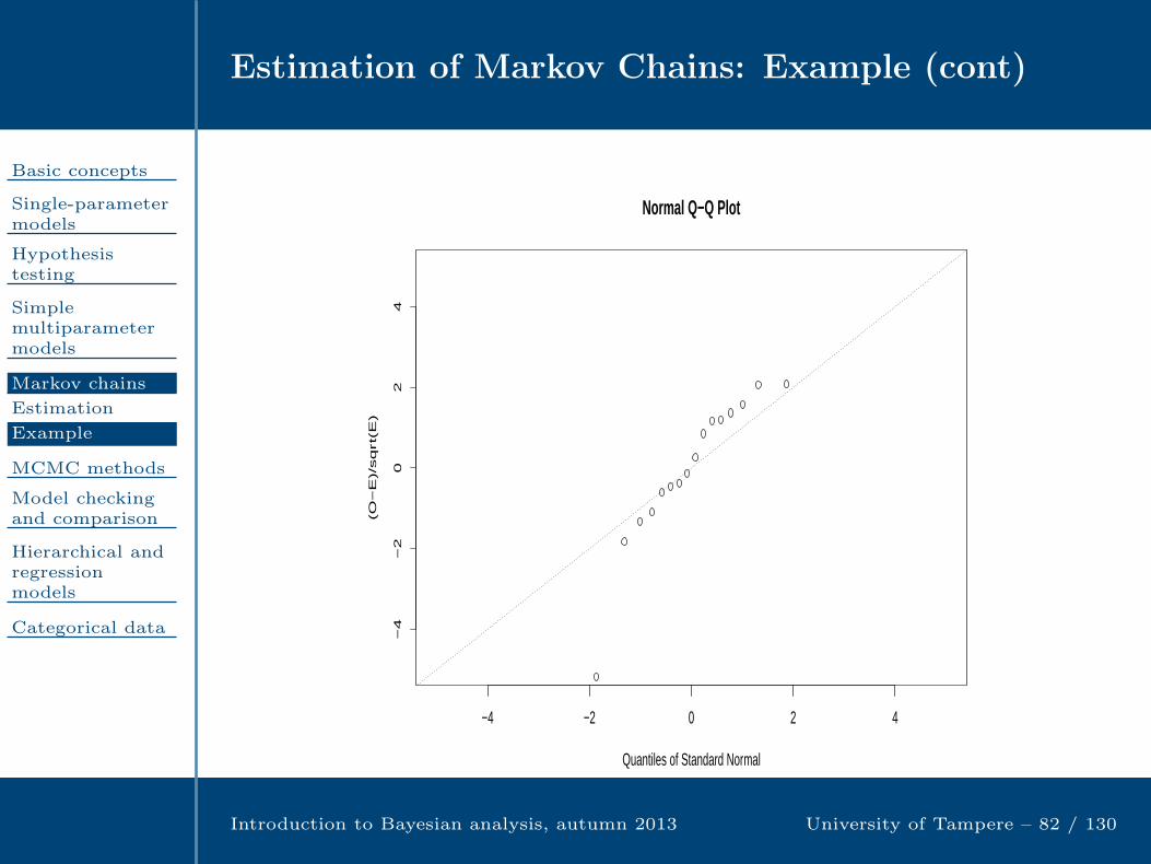
Estimation of Markov Chains: Example (cont)
Basic concepts
Single-parametermodels
Hypothesistesting
Simplemultiparametermodels
Markov chains
Estimation
Example
MCMC methods
Model checkingand comparison
Hierarchical andregressionmodels
Categorical data
Introduction to Bayesian analysis, autumn 2013 University of Tampere – 82 / 130
−4 −2 0 2 4
−4
−2
02
4
Normal Q−Q Plot
Quantiles of Standard Normal
(O−
E)/
sq
rt(
E)
Figure 5: Normal probability plot of normalized deviations
MCMC methods
Basic concepts
Single-parametermodels
Hypothesistesting
Simplemultiparametermodels
Markov chains
MCMC methods
Gibbs sampler
Metropolisalgorithm
Example
Metropolis-Hastings
Convergence
Model checkingand comparison
Hierarchical andregressionmodels
Categorical data
Introduction to Bayesian analysis, autumn 2013 University of Tampere – 83 / 130
MCMC methods
Basic concepts
Single-parametermodels
Hypothesistesting
Simplemultiparametermodels
Markov chains
MCMC methods
Gibbs sampler
Metropolisalgorithm
Example
Metropolis-Hastings
Convergence
Model checkingand comparison
Hierarchical andregressionmodels
Categorical data
Introduction to Bayesian analysis, autumn 2013 University of Tampere – 84 / 130
In the following, we will introduce computationally intensivemethods based on Markov chains which can be used in thesimulation of multivariate distributions. These are calledMarkov Chain Monte Carlo (MCMC) methods, and they areespecially useful in the computations of Bayesian statistics. Thegeneral idea is to generate a time-reversible Markov chain witha desired stationary distribution.

MCMC methods
Basic concepts
Single-parametermodels
Hypothesistesting
Simplemultiparametermodels
Markov chains
MCMC methods
Gibbs sampler
Metropolisalgorithm
Example
Metropolis-Hastings
Convergence
Model checkingand comparison
Hierarchical andregressionmodels
Categorical data
Introduction to Bayesian analysis, autumn 2013 University of Tampere – 84 / 130
In the following, we will introduce computationally intensivemethods based on Markov chains which can be used in thesimulation of multivariate distributions. These are calledMarkov Chain Monte Carlo (MCMC) methods, and they areespecially useful in the computations of Bayesian statistics. Thegeneral idea is to generate a time-reversible Markov chain witha desired stationary distribution.
We will assume that target distribution is discrete, so that wecan apply the theory of discrete state-space Markov chains.However, MCMC methods are often applied to continuousdistributions, so that their proper treatment would require thetheory of general state-space Markov chains. But sincecontinuous distributions can be approximated by discrete oneswith arbitrary accuracy, we can content ourselves with thetheory presented by far.
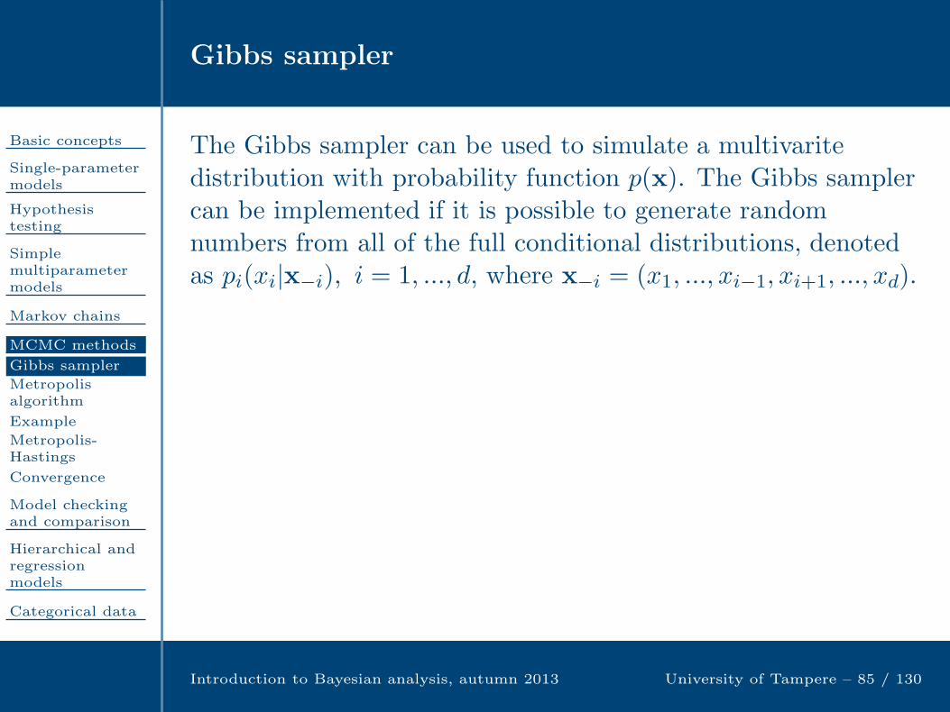
Gibbs sampler
Basic concepts
Single-parametermodels
Hypothesistesting
Simplemultiparametermodels
Markov chains
MCMC methods
Gibbs sampler
Metropolisalgorithm
Example
Metropolis-Hastings
Convergence
Model checkingand comparison
Hierarchical andregressionmodels
Categorical data
Introduction to Bayesian analysis, autumn 2013 University of Tampere – 85 / 130
The Gibbs sampler can be used to simulate a multivaritedistribution with probability function p(x). The Gibbs samplercan be implemented if it is possible to generate randomnumbers from all of the full conditional distributions, denotedas pi(xi|x−i), i = 1, ..., d, where x−i = (x1, ..., xi−1, xi+1, ..., xd).
Gibbs sampler
Basic concepts
Single-parametermodels
Hypothesistesting
Simplemultiparametermodels
Markov chains
MCMC methods
Gibbs sampler
Metropolisalgorithm
Example
Metropolis-Hastings
Convergence
Model checkingand comparison
Hierarchical andregressionmodels
Categorical data
Introduction to Bayesian analysis, autumn 2013 University of Tampere – 85 / 130
The Gibbs sampler can be used to simulate a multivaritedistribution with probability function p(x). The Gibbs samplercan be implemented if it is possible to generate randomnumbers from all of the full conditional distributions, denotedas pi(xi|x−i), i = 1, ..., d, where x−i = (x1, ..., xi−1, xi+1, ..., xd).
The algorithm is implemented so that one first chooses theinitial value vector x0 = (x01, ..., x
0d). After generating the
random vectors x1, ...,xt, the vector xt+1 is generatedcomponentwise as follows:
Generate xt+11 from p1(x1|xt2, ..., xtd)
Generate xt+12 from p2(x2|xt+1
1 , xt3, ..., xtd)
Generate xt+13 from p3(x3|xt+1
1 , xt+12 , xt4, ..., x
td)
... Generate xt+1
d from pd(xd|xt+11 , xt+1
2 , ..., xt+1d−1)

Gibbs sampler (cont)
Basic concepts
Single-parametermodels
Hypothesistesting
Simplemultiparametermodels
Markov chains
MCMC methods
Gibbs sampler
Metropolisalgorithm
Example
Metropolis-Hastings
Convergence
Model checkingand comparison
Hierarchical andregressionmodels
Categorical data
Introduction to Bayesian analysis, autumn 2013 University of Tampere – 86 / 130
The algorithm produces a Markov chain, since the distributionof x(t+1) is independent of x0, ...,x(t−1) given xt. It is timehomogenous, since the transition probabilites are based on thedistributions pj(xj |x−j) all the time. The chain is notnecessarily irreducible, but it is so if the set x : p(x) > 0 is’sufficiently’ connected enabling the process to move to allpoints of the state space.
We show next that p(x) fulfils the detailed balance condition
p(x) Pr(Xt+1 = x∗|Xt = x) = p(x∗) Pr(Xt+1 = x|Xt = x∗),
where x = (x1, ..., xj, ..., xd) and x∗ = (x1, ..., x∗j , ..., xd). For the
moment we consider that one time step corresponds tochanging only one component of x.

Gibbs sampler (cont)
Basic concepts
Single-parametermodels
Hypothesistesting
Simplemultiparametermodels
Markov chains
MCMC methods
Gibbs sampler
Metropolisalgorithm
Example
Metropolis-Hastings
Convergence
Model checkingand comparison
Hierarchical andregressionmodels
Categorical data
Introduction to Bayesian analysis, autumn 2013 University of Tampere – 87 / 130
We obtain that
p(x) Pr(Xt+1 = x∗|Xt = x) = p(x)pj(x∗j |x−j) = p(x)
p(x∗)
p(x−j)
= p(x∗)p(x)
p(x−j)= p(x∗)pj(xj |x−j)
= p(x∗) Pr(Xt+1 = x|Xt = x∗);
thus p(x) is a stationary distribution.
Irreducibility implies the uniqueness of the stationarydistribution. The chain is also positively recurrent, sincetransient and null recurrent chains do not posses a stationarydistribution. Further, it is aperiodic, since the new value can bethe same as the old. It follows from these properties that thechain is ergodic.

Metropolis algorithm
Basic concepts
Single-parametermodels
Hypothesistesting
Simplemultiparametermodels
Markov chains
MCMC methods
Gibbs sampler
Metropolisalgorithm
Example
Metropolis-Hastings
Convergence
Model checkingand comparison
Hierarchical andregressionmodels
Categorical data
Introduction to Bayesian analysis, autumn 2013 University of Tampere – 88 / 130
The Metropolis algorithm is different from Gibbs sampling inthat it does not require ability to generate random variatesfrom conditional distributions. It is sufficient to know theprobability function (or density) of the target density upto aconstant of proportionality.
Assume that we want to simulate a distribution withprobability function p(x) where x may be scalar or vector. Weneed to define a jumping distribution (or proposal distribution)J(y|x) from which a proposal y may be generated when thecurrent value is x. In the Metropolis algorithm it is assumedthat J(y|x) = J(x|y).

Metropolis algorithm (cont)
Basic concepts
Single-parametermodels
Hypothesistesting
Simplemultiparametermodels
Markov chains
MCMC methods
Gibbs sampler
Metropolisalgorithm
Example
Metropolis-Hastings
Convergence
Model checkingand comparison
Hierarchical andregressionmodels
Categorical data
Introduction to Bayesian analysis, autumn 2013 University of Tampere – 89 / 130
An initial value x0 is first generated. After generating x0, ..., xt,the new value xt+1 is obtained as follows: 1) A new proposal yis generated from J(y|x). The new value y is accepted withprobability
min
(1,p(y)
p(xt)
).
2) If the new value is accepted, we set xt+1 = y, otherwise theold value is kept, so that xt+1 = xt.
The Metropolis algorithm produces a Markov chain, since thedistribution of the new value xt+1 only depends on the currentvalue xt. The chain is also time-homogenous, since thetransition probabilities are based on the jumping distributionJ(y|x), which is not changed during the simulation. Further, itis irreducible if J(y|x) is so chosen that the chain may reach allpoints of the state space.

Metropolis algorithm (cont)
Basic concepts
Single-parametermodels
Hypothesistesting
Simplemultiparametermodels
Markov chains
MCMC methods
Gibbs sampler
Metropolisalgorithm
Example
Metropolis-Hastings
Convergence
Model checkingand comparison
Hierarchical andregressionmodels
Categorical data
Introduction to Bayesian analysis, autumn 2013 University of Tampere – 90 / 130
Next we show that p(x) fulfils the detailed balance condition.Let x and x∗ be two points in the state space such thatp(x∗) ≤ p(x). Then
p(x) Pr(Xt+1 = x∗|Xt = x) = p(x)J(x∗|x)p(x∗)
p(x)
= p(x∗)J(x|x∗)= p(x∗) Pr(Xt+1 = x|Xt = x∗).
Thus, p(x) is the stationary distribution and the chain ispositively recurrent. Further, since it is also aperiodic, it isergodic.

Metropolis algorithm (cont)
Basic concepts
Single-parametermodels
Hypothesistesting
Simplemultiparametermodels
Markov chains
MCMC methods
Gibbs sampler
Metropolisalgorithm
Example
Metropolis-Hastings
Convergence
Model checkingand comparison
Hierarchical andregressionmodels
Categorical data
Introduction to Bayesian analysis, autumn 2013 University of Tampere – 91 / 130
It is said that a Markov chain mixes slowly if it moves slowlyaround the support of p(x). Then there is strongautocorrelation between the consequtive observations, and themean converges slowly to the theoretical mean of the stationarydistribution.
There are two possible reasons for this problem. First, if thedeviation of the jumping distribution is too small for somecomponent, the chain moves slowly with respect to thatcomponent. On the other hand, if the deviation is too large,new proposals are rarely accepted and the chain remains long inthe same position.
It is possible to optimize the jumping distribution. If thejumping distribution is a d-dimensional normal distribution,then its optimal covariance matrix is c2Σ where c ≈ 2.4/
√d and
Σ is the covariance matrix of the target distribution.

Metropolis algorithm: Example
Basic concepts
Single-parametermodels
Hypothesistesting
Simplemultiparametermodels
Markov chains
MCMC methods
Gibbs sampler
Metropolisalgorithm
Example
Metropolis-Hastings
Convergence
Model checkingand comparison
Hierarchical andregressionmodels
Categorical data
Introduction to Bayesian analysis, autumn 2013 University of Tampere – 92 / 130
Let us consider a two-parameter Weibull distribution with thedensity
f(x;β, δ) =δ
βδxδ−1 exp
−(x
β
)δ, x, β, δ > 0.
With a random sample y1, ..., yn the likelihood is
p(y|θ) = δn
βnδ
(∏
i
yi
)δ−1
exp
−∑
i
(yiβ
)δ.
By choosing p(β, δ) ∝ 1/(βδ) as the prior, the posterior becomes
p(β, δ|y) ∝ δn−1
βnδ+1
(∏
i
yi
)δ−1
exp
−∑
i
(yiβ
)δ.

Metropolis algorithm: Example (cont)
Basic concepts
Single-parametermodels
Hypothesistesting
Simplemultiparametermodels
Markov chains
MCMC methods
Gibbs sampler
Metropolisalgorithm
Example
Metropolis-Hastings
Convergence
Model checkingand comparison
Hierarchical andregressionmodels
Categorical data
Introduction to Bayesian analysis, autumn 2013 University of Tampere – 93 / 130
It would be possible to derive the full conditional posteriordistributions and simulate the posterior distribution usingGibbs sampling. We could generate random numbers from theconditional distributions using adaptive rejection sampling.However, it is here simpler to apply the Metropolis algorithm.
To illustrate the estimation, we generate an artificial data set of100 observations from the Weibull(0.3,10) distribution. Figure 6shows a simulated Markov chain with 10000 iterations, startingfrom the initial values δ = β = 1. As a jumping distribution weuse the bivariate normal distribution, the mean vector beingthe ’old’ vector and the covariance matrix diag(0.01, 10).
The figure shows that the chain converges to its stationarydistribution rapidly but the chain for β seems to mix poorly.
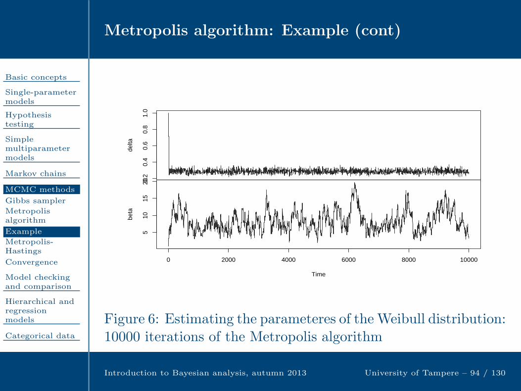
Metropolis algorithm: Example (cont)
Basic concepts
Single-parametermodels
Hypothesistesting
Simplemultiparametermodels
Markov chains
MCMC methods
Gibbs sampler
Metropolisalgorithm
Example
Metropolis-Hastings
Convergence
Model checkingand comparison
Hierarchical andregressionmodels
Categorical data
Introduction to Bayesian analysis, autumn 2013 University of Tampere – 94 / 130
0.2
0.4
0.6
0.8
1.0
delta
510
1520
0 2000 4000 6000 8000 10000
beta
Time
Figure 6: Estimating the parameteres of the Weibull distribution:10000 iterations of the Metropolis algorithm

Metropolis algorithm: Example (cont)
Basic concepts
Single-parametermodels
Hypothesistesting
Simplemultiparametermodels
Markov chains
MCMC methods
Gibbs sampler
Metropolisalgorithm
Example
Metropolis-Hastings
Convergence
Model checkingand comparison
Hierarchical andregressionmodels
Categorical data
Introduction to Bayesian analysis, autumn 2013 University of Tampere – 95 / 130
Next we simulate 10000 new observations using the optimalcovariance matrix 2.42Σ/2 where Σ is the covariance matrix ofthe target distribution, estimated using the most recentsimulations of the original chain. As an initial value we use thelast simulated vector of the first chain. On the basis of Figure 7the mixing is more rapid now. Figure 8 shows the graphs of the2.5%, 50% and 97% cumulative quantiles.

Metropolis algorithm: Example (cont)
Basic concepts
Single-parametermodels
Hypothesistesting
Simplemultiparametermodels
Markov chains
MCMC methods
Gibbs sampler
Metropolisalgorithm
Example
Metropolis-Hastings
Convergence
Model checkingand comparison
Hierarchical andregressionmodels
Categorical data
Introduction to Bayesian analysis, autumn 2013 University of Tampere – 96 / 130
0.25
0.30
0.35
delta
510
1520
25
0 2000 4000 6000 8000 10000
beta
Time
Figure 7: Estimating the parameteres of the Weibull distribution:10000 further iterations of the Metropolis algorithm

Metropolis algorithm: Example (cont)
Basic concepts
Single-parametermodels
Hypothesistesting
Simplemultiparametermodels
Markov chains
MCMC methods
Gibbs sampler
Metropolisalgorithm
Example
Metropolis-Hastings
Convergence
Model checkingand comparison
Hierarchical andregressionmodels
Categorical data
Introduction to Bayesian analysis, autumn 2013 University of Tampere – 97 / 130
0 2000 4000 6000 8000 10000
0.24
0.26
0.28
0.30
0.32
Iterations
delta
0 2000 4000 6000 8000 10000
510
15
Iterations
beta
Figure 8: 2.5%, 50% and 97% cumulative quantiles of 10000posterior simulations
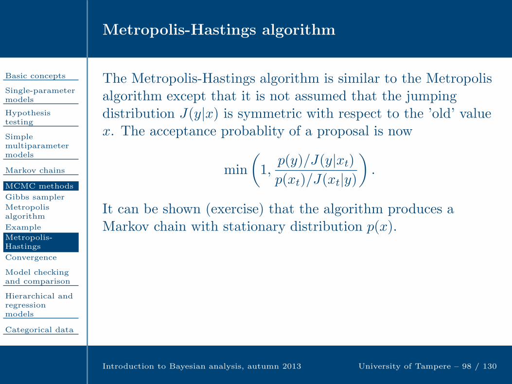
Metropolis-Hastings algorithm
Basic concepts
Single-parametermodels
Hypothesistesting
Simplemultiparametermodels
Markov chains
MCMC methods
Gibbs sampler
Metropolisalgorithm
Example
Metropolis-Hastings
Convergence
Model checkingand comparison
Hierarchical andregressionmodels
Categorical data
Introduction to Bayesian analysis, autumn 2013 University of Tampere – 98 / 130
The Metropolis-Hastings algorithm is similar to the Metropolisalgorithm except that it is not assumed that the jumpingdistribution J(y|x) is symmetric with respect to the ’old’ valuex. The acceptance probablity of a proposal is now
min
(1,p(y)/J(y|xt)p(xt)/J(xt|y)
).
It can be shown (exercise) that the algorithm produces aMarkov chain with stationary distribution p(x).
Detecting convergence
Basic concepts
Single-parametermodels
Hypothesistesting
Simplemultiparametermodels
Markov chains
MCMC methods
Gibbs sampler
Metropolisalgorithm
Example
Metropolis-Hastings
Convergence
Model checkingand comparison
Hierarchical andregressionmodels
Categorical data
Introduction to Bayesian analysis, autumn 2013 University of Tampere – 99 / 130
Markov Chain simulation should be continued until reachingthe stationary distribution, and after this until reliableestimates for the summary statistics of the stationarydistribution have been obtained. The iterations before theconvergence are usually disregarded as a burn-in phase.
In practice, convergence to stationary distribution can bedetected by studying various time series plots, such as traceplots, and plots of cumulative summary statistics andautoregression functions.
However, it is usually more reliable to also use convergencediagnostics. Geweke’s diagnostic is based on comparing themeans of the beginning and last parts of the chain. In thefollowing, we will introduce Gelman and Rubin’s diagnostic,which is based on comparing several simulated chains.
Gelman and Rubin’s diagnostic
Basic concepts
Single-parametermodels
Hypothesistesting
Simplemultiparametermodels
Markov chains
MCMC methods
Gibbs sampler
Metropolisalgorithm
Example
Metropolis-Hastings
Convergence
Model checkingand comparison
Hierarchical andregressionmodels
Categorical data
Introduction to Bayesian analysis, autumn 2013 University of Tampere – 100 / 130
Suppose we have simulated m chains of n iterations (afterremoving the burn-in phase). We denote the simulations byψij (i = 1, ..., n; j = 1, ..., n), and compute B and W , thebetween- and within-sequence variances:
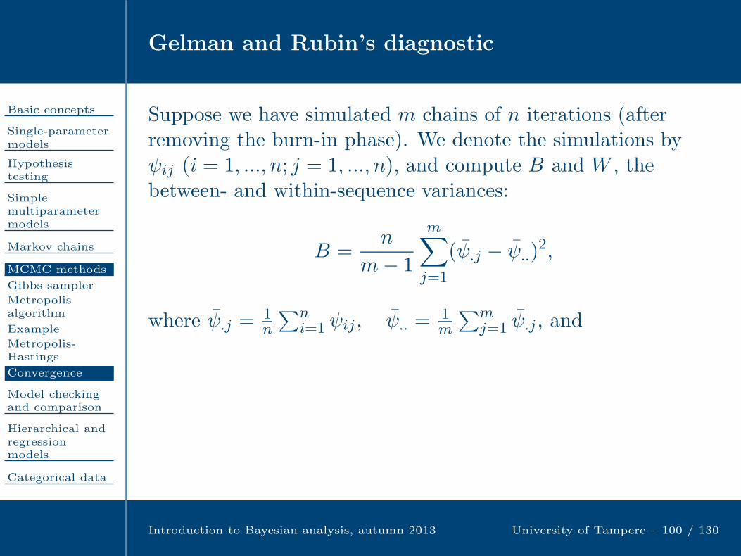
B =n
m− 1
m∑
j=1
(ψ.j − ψ..)2,
where ψ.j =1n
∑ni=1 ψij , ψ.. =
1m
∑mj=1 ψ.j , and
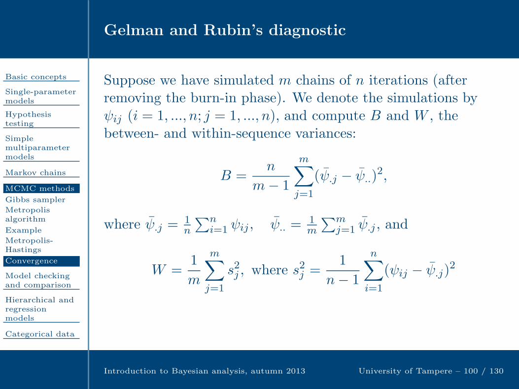
W =1
m
m∑
j=1
s2j , where s2j =
1
n− 1
n∑
i=1
(ψij − ψ.j)2
We can estimate the posterior variance Var(ψ|y) by the
weighted average Var+(ψ|y) = n−1
n W + 1nB.

Gelman and Rubin’s diagnostic (cont)
Basic concepts
Single-parametermodels
Hypothesistesting
Simplemultiparametermodels
Markov chains
MCMC methods
Gibbs sampler
Metropolisalgorithm
Example
Metropolis-Hastings
Convergence
Model checkingand comparison
Hierarchical andregressionmodels
Categorical data
Introduction to Bayesian analysis, autumn 2013 University of Tampere – 101 / 130
The quantity Var+(ψ|y) overestimates the posterior variance if
the starting values are overdispersed, but is unbiased understationarity. On the other hand, W underestimates posteriorvariance for any finite n because the individual sequences havenot had time to range over all of the target distribution.
We may monitor convergence using the potential scale factor
R =
√Var
+(ψ|y)W
which tells by which factor the posterior deviation estimate canbe decreased if simulation is continued. Simulation should becontinued until R is close to 1 for each parameter ψ. In mostpractical cases, values below 1.1 would be acceptable.

Gelman and Rubin’s diagnostic: Example
Basic concepts
Single-parametermodels
Hypothesistesting
Simplemultiparametermodels
Markov chains
MCMC methods
Gibbs sampler
Metropolisalgorithm
Example
Metropolis-Hastings
Convergence
Model checkingand comparison
Hierarchical andregressionmodels
Categorical data
Introduction to Bayesian analysis, autumn 2013 University of Tampere – 102 / 130
To illustrate the use of the diagnostic, we continue our exampleon the Weibull distribution. We generate 5 chains of length1000 using random initial values. After removing the first 500simulations from each chain, we obtain the followingdiagnostics. Also a multivariate version of the diagnostic iscomputed. Here, gelman.diag is a function in R package codaand SIMS is an mcmc object containing the chains.
1> gelman.diag(SIMS)
Potential scale reduction factors:
Point est. Upper C.I.
delta 1.00 1.01
beta 1.01 1.02
Multivariate psrf
1.01
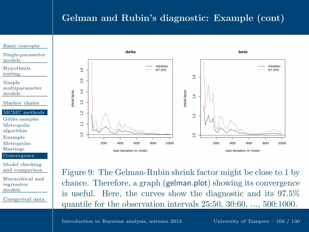
Gelman and Rubin’s diagnostic: Example (cont)
Basic concepts
Single-parametermodels
Hypothesistesting
Simplemultiparametermodels
Markov chains
MCMC methods
Gibbs sampler
Metropolisalgorithm
Example
Metropolis-Hastings
Convergence
Model checkingand comparison
Hierarchical andregressionmodels
Categorical data
Introduction to Bayesian analysis, autumn 2013 University of Tampere – 103 / 130
200 400 600 800 1000
1.0
1.1
1.2
1.3
1.4
1.5
1.6
last iteration in chain
shrin
k fa
ctor
median97.5%
delta
200 400 600 800 1000
1.0
1.2
1.4
1.6
last iteration in chain
shrin
k fa
ctor
median97.5%
beta
Figure 9: The Gelman-Rubin shrink factor might be close to 1 bychance. Therefore, a graph (gelman.plot) showing its convergenceis useful. Here, the curves show the diagnostic and its 97.5%quantile for the observation intervals 25:50, 30:60, ..., 500:1000.
Model checking and comparison
Basic concepts
Single-parametermodels
Hypothesistesting
Simplemultiparametermodels
Markov chains
MCMC methods
Model checkingand comparison
Residuals
Example
Predictive checks
p-values
Example 1
Example 2
Deviance
DIC
Example
Hierarchical andregressionmodels
Categorical data
Introduction to Bayesian analysis, autumn 2013 University of Tampere – 104 / 130
Model checking and comparison
Basic concepts
Single-parametermodels
Hypothesistesting
Simplemultiparametermodels
Markov chains
MCMC methods
Model checkingand comparison
Residuals
Example
Predictive checks
p-values
Example 1
Example 2
Deviance
DIC
Example
Hierarchical andregressionmodels
Categorical data
Introduction to Bayesian analysis, autumn 2013 University of Tampere – 105 / 130
The conclusions of a Bayesian analysis are conditional on thechosen probability model. Therefore, it is essential to checkthat the model is a reasonable approximation to reality. Modelchecking can be done with respect to outliers, samplingdistribution, prior distribution, link function, covariates and soon.
We can distinguish three aspects of modelling:
Criticism: exploratory checking of a single model Extension: embedding a model in a larger model Comparison: comparing candidate models in terms of their
fit and predictive power

Residuals
Basic concepts
Single-parametermodels
Hypothesistesting
Simplemultiparametermodels
Markov chains
MCMC methods
Model checkingand comparison
Residuals
Example
Predictive checks
p-values
Example 1
Example 2
Deviance
DIC
Example
Hierarchical andregressionmodels
Categorical data
Introduction to Bayesian analysis, autumn 2013 University of Tampere – 106 / 130
A widely used and useful technique for model checking isplotting residuals. They help, for example, detect outliers,autocorrelation and problems in distributional assumptions.They measure the deviation between observations andestimated expected values.

Residuals
Basic concepts
Single-parametermodels
Hypothesistesting
Simplemultiparametermodels
Markov chains
MCMC methods
Model checkingand comparison
Residuals
Example
Predictive checks
p-values
Example 1
Example 2
Deviance
DIC
Example
Hierarchical andregressionmodels
Categorical data
Introduction to Bayesian analysis, autumn 2013 University of Tampere – 106 / 130
A widely used and useful technique for model checking isplotting residuals. They help, for example, detect outliers,autocorrelation and problems in distributional assumptions.They measure the deviation between observations andestimated expected values.
A Pearson residual is defined as
ri(θ) =yi − E(yi|θ)√
Var(yi|θ).
In classical analysis, θ is replaced by its fitted value, while inBayesian analysis the residuals have a posterior distribution.

Residuals
Basic concepts
Single-parametermodels
Hypothesistesting
Simplemultiparametermodels
Markov chains
MCMC methods
Model checkingand comparison
Residuals
Example
Predictive checks
p-values
Example 1
Example 2
Deviance
DIC
Example
Hierarchical andregressionmodels
Categorical data
Introduction to Bayesian analysis, autumn 2013 University of Tampere – 106 / 130
A widely used and useful technique for model checking isplotting residuals. They help, for example, detect outliers,autocorrelation and problems in distributional assumptions.They measure the deviation between observations andestimated expected values.
A Pearson residual is defined as
ri(θ) =yi − E(yi|θ)√
Var(yi|θ).
In classical analysis, θ is replaced by its fitted value, while inBayesian analysis the residuals have a posterior distribution.
Example. We consider the child heart surgery data in Table 1.Figure 10 shows the box plot of Pearson residuals assumingthat yi ∼ Bin(θ,mj). Hospital H appears to be an outlier.

Residuals (cont)
Basic concepts
Single-parametermodels
Hypothesistesting
Simplemultiparametermodels
Markov chains
MCMC methods
Model checkingand comparison
Residuals
Example
Predictive checks
p-values
Example 1
Example 2
Deviance
DIC
Example
Hierarchical andregressionmodels
Categorical data
Introduction to Bayesian analysis, autumn 2013 University of Tampere – 107 / 130
E A D G L F I C J B K H
−4
−2
02
46
Figure 10: Box plot of Pearson residuals for heart surgery data
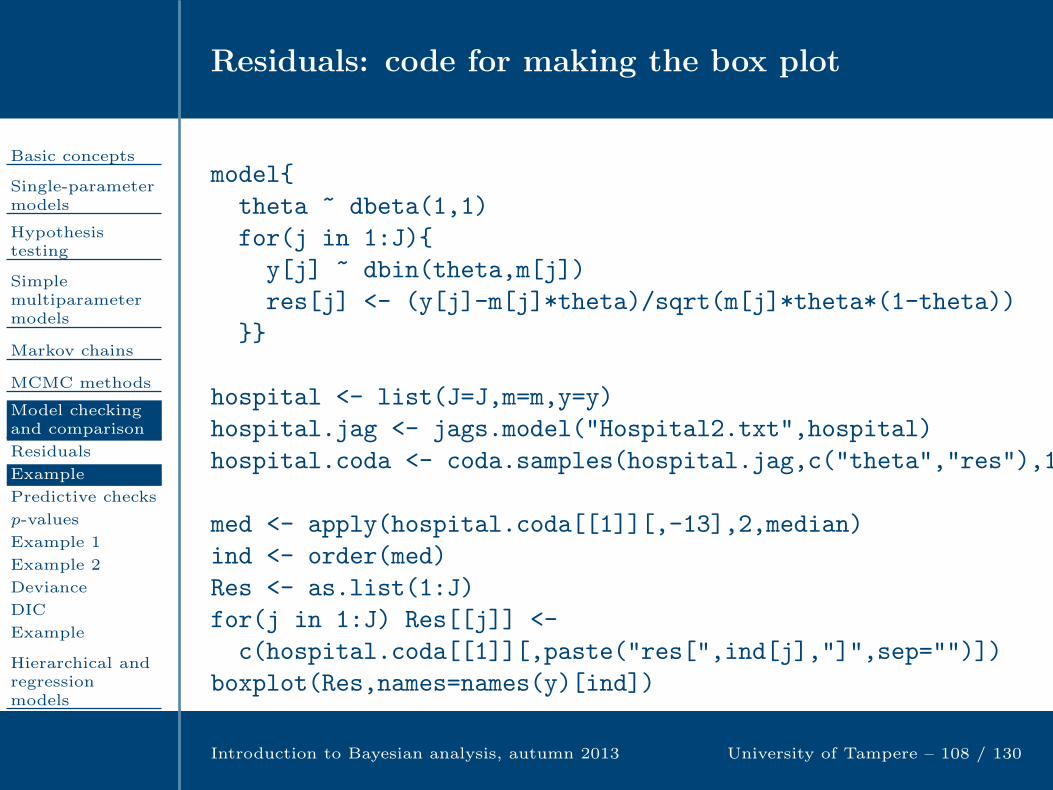
Residuals: code for making the box plot
Basic concepts
Single-parametermodels
Hypothesistesting
Simplemultiparametermodels
Markov chains
MCMC methods
Model checkingand comparison
Residuals
Example
Predictive checks
p-values
Example 1
Example 2
Deviance
DIC
Example
Hierarchical andregressionmodels
Categorical data
Introduction to Bayesian analysis, autumn 2013 University of Tampere – 108 / 130
model
theta ~ dbeta(1,1)
for(j in 1:J)
y[j] ~ dbin(theta,m[j])
res[j] <- (y[j]-m[j]*theta)/sqrt(m[j]*theta*(1-theta))
hospital <- list(J=J,m=m,y=y)
hospital.jag <- jags.model("Hospital2.txt",hospital)
hospital.coda <- coda.samples(hospital.jag,c("theta","res"),10000)
med <- apply(hospital.coda[[1]][,-13],2,median)
ind <- order(med)
Res <- as.list(1:J)
for(j in 1:J) Res[[j]] <-
c(hospital.coda[[1]][,paste("res[",ind[j],"]",sep="")])
boxplot(Res,names=names(y)[ind])

Predictive checks and Bayesian p-values
Basic concepts
Single-parametermodels
Hypothesistesting
Simplemultiparametermodels
Markov chains
MCMC methods
Model checkingand comparison
Residuals
Example
Predictive checks
p-values
Example 1
Example 2
Deviance
DIC
Example
Hierarchical andregressionmodels
Categorical data
Introduction to Bayesian analysis, autumn 2013 University of Tampere – 109 / 130
Residuals are examples of statistics which measure thediscrepancy between the data and the assumed model. Thesestatistics are usually easy to calculate, but we beed a method todetermine if the observed discrepancy is significant. Here, wemay use so-called Bayesian p-values obtained by simulating theposterior predictive distribution of the test statistic.
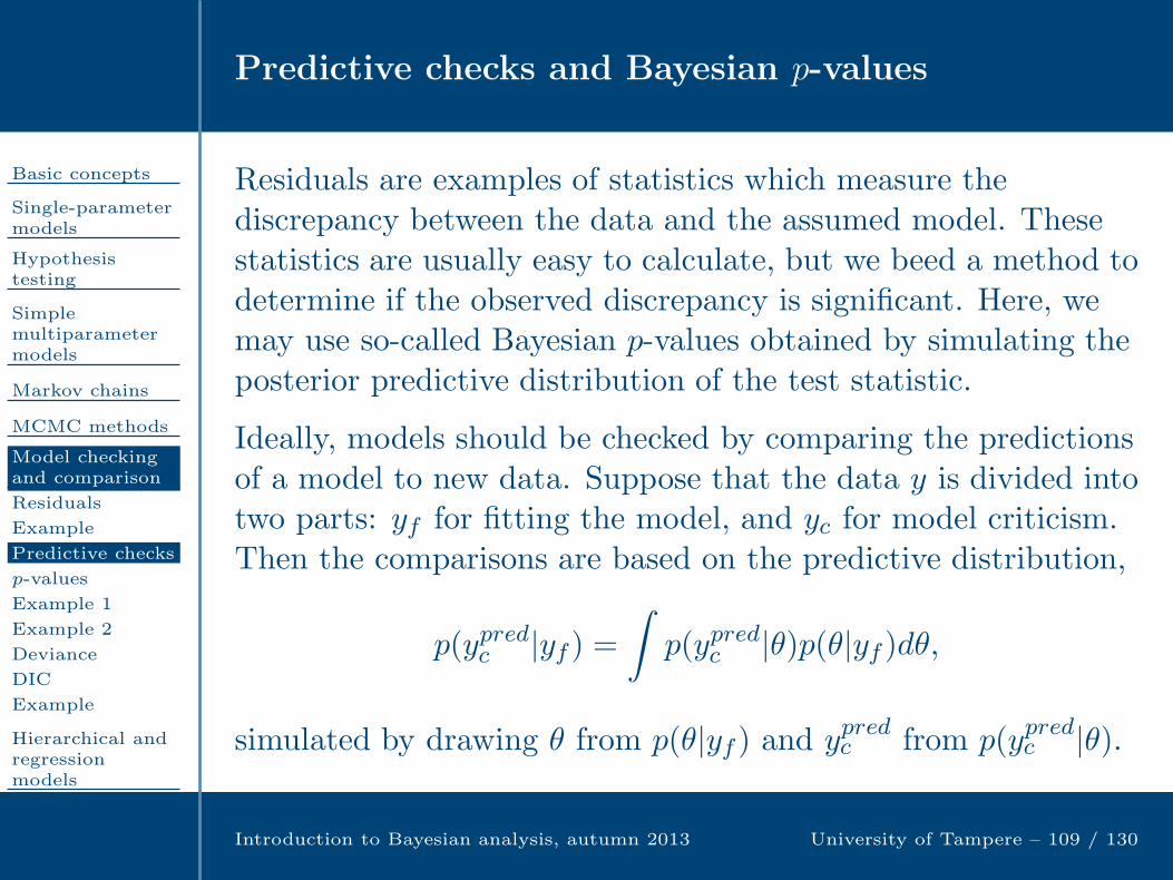
Ideally, models should be checked by comparing the predictionsof a model to new data. Suppose that the data y is divided intotwo parts: yf for fitting the model, and yc for model criticism.Then the comparisons are based on the predictive distribution,
p(ypredc |yf ) =∫p(ypredc |θ)p(θ|yf )dθ,
simulated by drawing θ from p(θ|yf ) and ypredc from p(ypredc |θ).

Predictive checks and Bayesian p-values (cont)
Basic concepts
Single-parametermodels
Hypothesistesting
Simplemultiparametermodels
Markov chains
MCMC methods
Model checkingand comparison
Residuals
Example
Predictive checks
p-values
Example 1
Example 2
Deviance
DIC
Example
Hierarchical andregressionmodels
Categorical data
Introduction to Bayesian analysis, autumn 2013 University of Tampere – 110 / 130
A function T (yc) is called a test statistic (Gelman et al., 2004)if it would have an extreme value if the data yc conflict with theassumed model. By choosing T (yc) = yci one can check forindividual outliers.
One can check whether T (yc) is extreme graphically or bycomputing the Bayesian p-value
p = Pr(T (ypredc ) ≤ T (yc)|yf ).
This can be obtained by drawing simulations ypredc from theposterior predictive distribution, and by calculating theproportion of cases where T (ypredc ) ≤ T (yc).
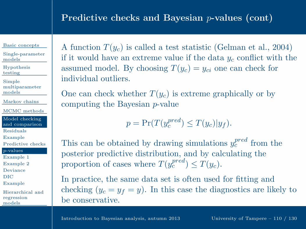
In practice, the same data set is often used for fitting andchecking (yc = yf = y). In this case the diagnostics are likely tobe conservative.
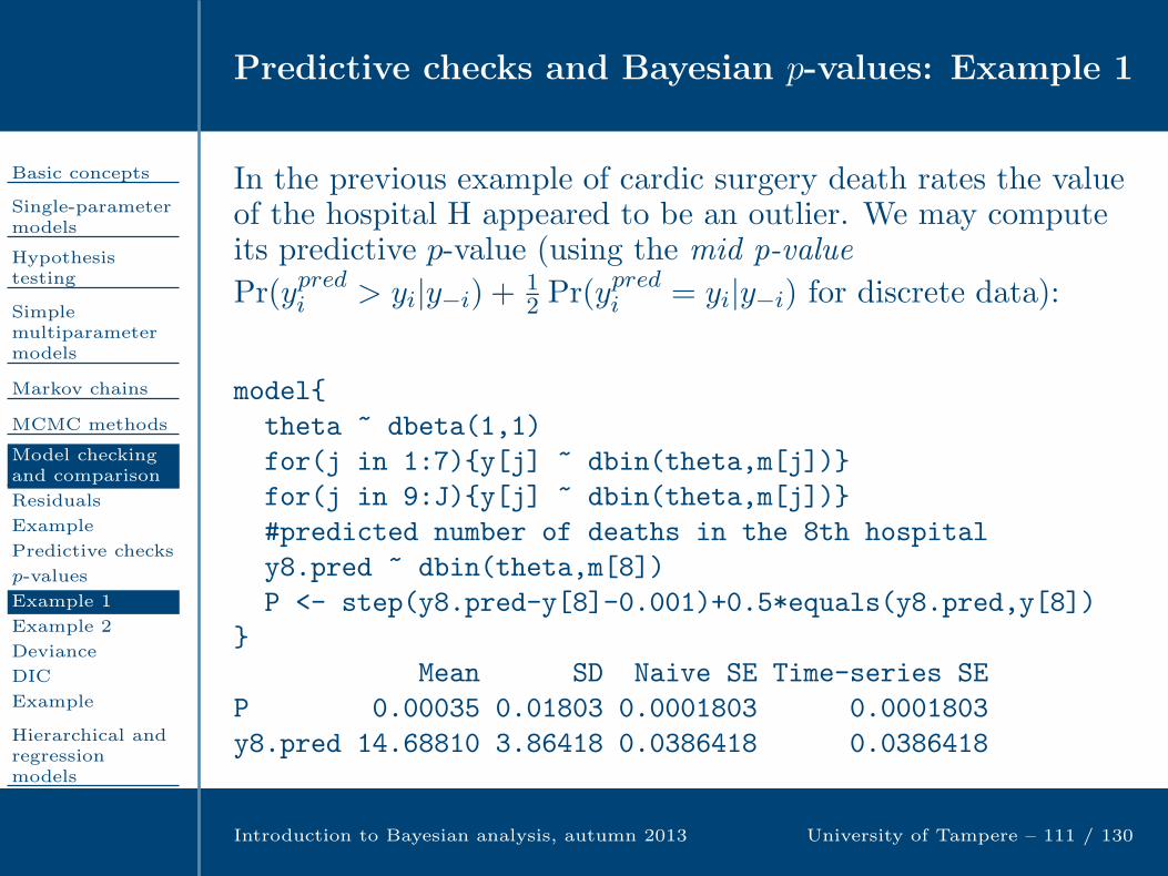
Predictive checks and Bayesian p-values: Example 1
Basic concepts
Single-parametermodels
Hypothesistesting
Simplemultiparametermodels
Markov chains
MCMC methods
Model checkingand comparison
Residuals
Example
Predictive checks
p-values
Example 1
Example 2
Deviance
DIC
Example
Hierarchical andregressionmodels
Categorical data
Introduction to Bayesian analysis, autumn 2013 University of Tampere – 111 / 130
In the previous example of cardic surgery death rates the valueof the hospital H appeared to be an outlier. We may computeits predictive p-value (using the mid p-value
Pr(ypredi > yi|y−i) +12 Pr(y
predi = yi|y−i) for discrete data):
model
theta ~ dbeta(1,1)
for(j in 1:7)y[j] ~ dbin(theta,m[j])
for(j in 9:J)y[j] ~ dbin(theta,m[j])
#predicted number of deaths in the 8th hospital
y8.pred ~ dbin(theta,m[8])
P <- step(y8.pred-y[8]-0.001)+0.5*equals(y8.pred,y[8])
Mean SD Naive SE Time-series SE
P 0.00035 0.01803 0.0001803 0.0001803
y8.pred 14.68810 3.86418 0.0386418 0.0386418

Predictive checks and Bayesian p-values: Example 2
Basic concepts
Single-parametermodels
Hypothesistesting
Simplemultiparametermodels
Markov chains
MCMC methods
Model checkingand comparison
Residuals
Example
Predictive checks
p-values
Example 1
Example 2
Deviance
DIC
Example
Hierarchical andregressionmodels
Categorical data
Introduction to Bayesian analysis, autumn 2013 University of Tampere – 112 / 130
We continue our study of the Newcomb data, and use thestatistics T1 = min(y) and T2 = (y(1) − y(n/2))/(y(n/4) − y(n/2)),where y(j) is the jth lowest value of y.
for(i in 1:n)
y[i] ~ dnorm(mu,tau)
yrep[i] ~ dnorm(mu,tau)
n.50 <- round(n/2)
n.25 <- round(n/4)
yrep.sort <- sort(yrep[])
T1.rep <- yrep.sort[1]
yrep.50 <- yrep.sort[n.50]
yrep.25 <- yrep.sort[n.25]
T2.rep <- (T1.rep-yrep.50)/(yrep.25-yrep.50)
P1 <- step(T1.rep-T1.obs)
P2 <- step(T2.rep-T2.obs)
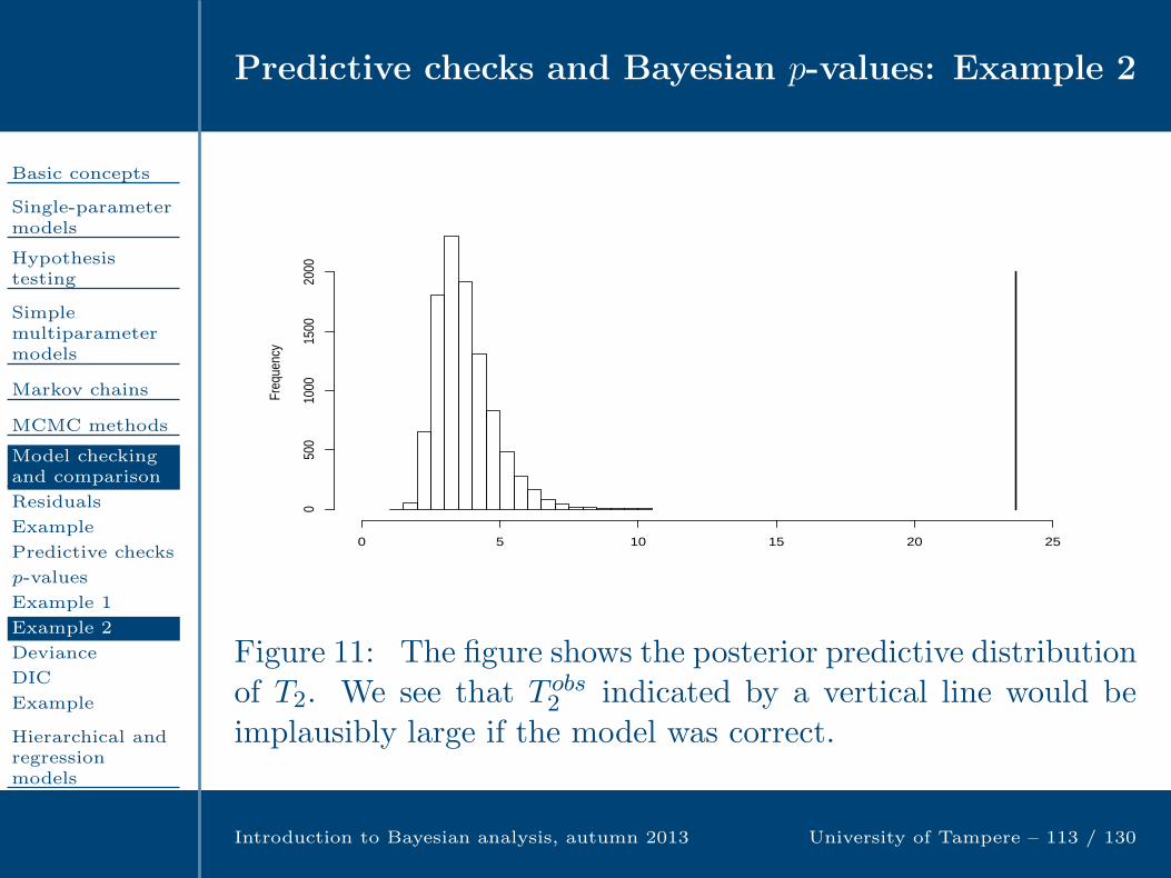
Predictive checks and Bayesian p-values: Example 2
Basic concepts
Single-parametermodels
Hypothesistesting
Simplemultiparametermodels
Markov chains
MCMC methods
Model checkingand comparison
Residuals
Example
Predictive checks
p-values
Example 1
Example 2
Deviance
DIC
Example
Hierarchical andregressionmodels
Categorical data
Introduction to Bayesian analysis, autumn 2013 University of Tampere – 113 / 130
Freq
uenc
y
0 5 10 15 20 25
050
010
0015
0020
00
Figure 11: The figure shows the posterior predictive distributionof T2. We see that T obs
2 indicated by a vertical line would beimplausibly large if the model was correct.

Model comparison using deviances
Basic concepts
Single-parametermodels
Hypothesistesting
Simplemultiparametermodels
Markov chains
MCMC methods
Model checkingand comparison
Residuals
Example
Predictive checks
p-values
Example 1
Example 2
Deviance
DIC
Example
Hierarchical andregressionmodels
Categorical data
Introduction to Bayesian analysis, autumn 2013 University of Tampere – 114 / 130
Model fit can be summarized with the deviance, defined as
D(θ) = −2 log p(y|θ)
where p(y|θ) is the likelihood function.

Model comparison using deviances
Basic concepts
Single-parametermodels
Hypothesistesting
Simplemultiparametermodels
Markov chains
MCMC methods
Model checkingand comparison
Residuals
Example
Predictive checks
p-values
Example 1
Example 2
Deviance
DIC
Example
Hierarchical andregressionmodels
Categorical data
Introduction to Bayesian analysis, autumn 2013 University of Tampere – 114 / 130
Model fit can be summarized with the deviance, defined as
D(θ) = −2 log p(y|θ)
where p(y|θ) is the likelihood function.To obtain a summarythat depends on y only, θ can be replaced with a point estimateθ, such as posterior mean. We obtain
D(θ) = −2 log p(y|θ).
This may give an over-optimistic picture of the model fit.
Model comparison using deviances
Basic concepts
Single-parametermodels
Hypothesistesting
Simplemultiparametermodels
Markov chains
MCMC methods
Model checkingand comparison
Residuals
Example
Predictive checks
p-values
Example 1
Example 2
Deviance
DIC
Example
Hierarchical andregressionmodels
Categorical data
Introduction to Bayesian analysis, autumn 2013 University of Tampere – 114 / 130
Model fit can be summarized with the deviance, defined as
D(θ) = −2 log p(y|θ)
where p(y|θ) is the likelihood function.To obtain a summarythat depends on y only, θ can be replaced with a point estimateθ, such as posterior mean. We obtain
D(θ) = −2 log p(y|θ).
This may give an over-optimistic picture of the model fit. Anatural Bayesian alternative is the posterior mean deviance
D = E(D(θ)|y).

Model comparison using deviances (cont)
Basic concepts
Single-parametermodels
Hypothesistesting
Simplemultiparametermodels
Markov chains
MCMC methods
Model checkingand comparison
Residuals
Example
Predictive checks
p-values
Example 1
Example 2
Deviance
DIC
Example
Hierarchical andregressionmodels
Categorical data
Introduction to Bayesian analysis, autumn 2013 University of Tampere – 115 / 130
It is easy to estimate D using posterior simulations θl:
ˆD =1
L
L∑
l=1
D(θl).
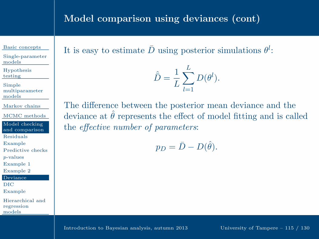
The difference between the posterior mean deviance and thedeviance at θ represents the effect of model fitting and is calledthe effective number of parameters:
pD = D −D(θ).
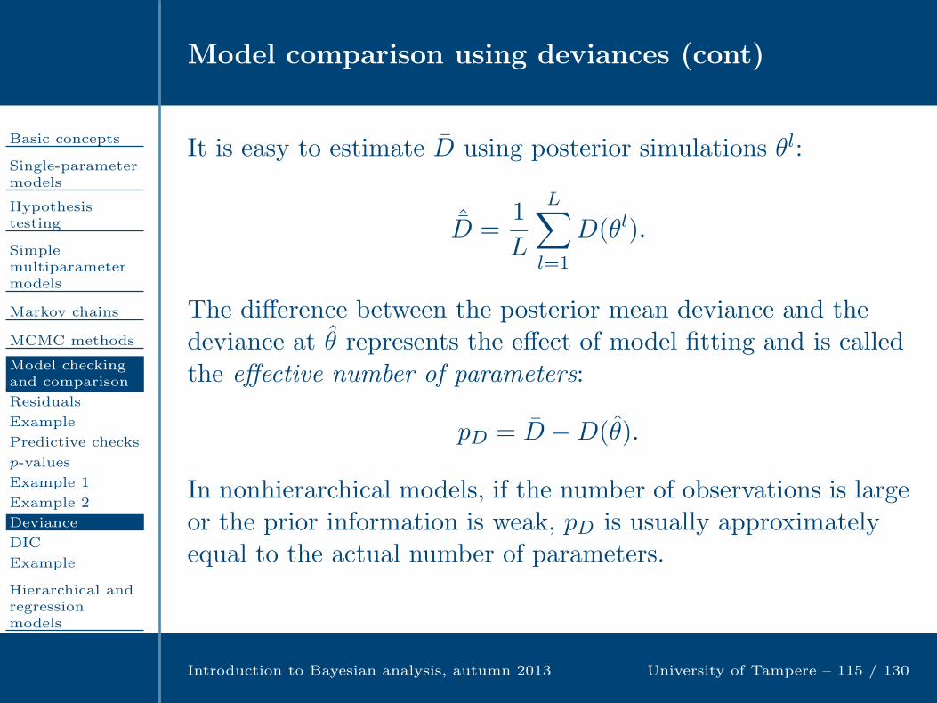
In nonhierarchical models, if the number of observations is largeor the prior information is weak, pD is usually approximatelyequal to the actual number of parameters.
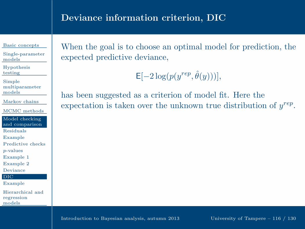
Deviance information criterion, DIC
Basic concepts
Single-parametermodels
Hypothesistesting
Simplemultiparametermodels
Markov chains
MCMC methods
Model checkingand comparison
Residuals
Example
Predictive checks
p-values
Example 1
Example 2
Deviance
DIC
Example
Hierarchical andregressionmodels
Categorical data
Introduction to Bayesian analysis, autumn 2013 University of Tampere – 116 / 130
When the goal is to choose an optimal model for prediction, theexpected predictive deviance,
E[−2 log(p(yrep, θ(y)))],
has been suggested as a criterion of model fit. Here theexpectation is taken over the unknown true distribution of yrep.
This can be approximated by the deviance information
criterion (DIC):
DIC = D(θ) + 2pD = D + pD.
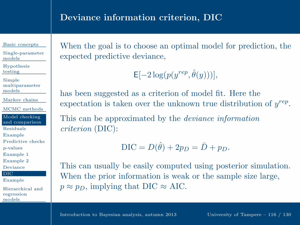
This can usually be easily computed using posterior simulation.When the prior information is weak or the sample size large,p ≈ pD, implying that DIC ≈ AIC.
Deviance information criterion (example)
Basic concepts
Single-parametermodels
Hypothesistesting
Simplemultiparametermodels
Markov chains
MCMC methods
Model checkingand comparison
Residuals
Example
Predictive checks
p-values
Example 1
Example 2
Deviance
DIC
Example
Hierarchical andregressionmodels
Categorical data
Introduction to Bayesian analysis, autumn 2013 University of Tampere – 117 / 130
We regress the incidence of pine processionary caterpillars on 8potential exploratory variables. (The data set is caterpillar in R
package bayess.) The response variable y is the log transform ofthe average number of nests per tree.
The explanatory variables:x1 altitude (in meters)x2 slope (in degrees)x3 number of pine trees in the areax4 height (in meters) of the tree sampled at the center of theareax5 orientation of the area (from 1 if southbound to 2 otherwise)x6 height (in meters) of the dominant treex7 number of vegetation stratax8 mix settlement index (from 1 if not mixed to 2 if mixed)

DIC example (cont)
Basic concepts
Single-parametermodels
Hypothesistesting
Simplemultiparametermodels
Markov chains
MCMC methods
Model checkingand comparison
Residuals
Example
Predictive checks
p-values
Example 1
Example 2
Deviance
DIC
Example
Hierarchical andregressionmodels
Categorical data
Introduction to Bayesian analysis, autumn 2013 University of Tampere – 118 / 130
#JAGS code
for(i in 1:n)
y[i] ~ dnorm(mu[i],tau)
mu[i] <- b0 +b[1]*X[i,1]+b[2]*X[i,2]+b[3]*X[i,3]+
b[4]*X[i,4]+b[5]*X[i,5]+b[6]*X[i,6]+
b[7]*X[i,7]+b[8]*X[i,8]
b0 ~ dnorm(0,0.001)
tau ~ dgamma(0.001,0.001)
for(j in 1:8)
b[j] ~ dnorm(0,0.001)
#R code
cp.jag <- jags.model("caterpillar.txt",data,n.chains=2)
cp.coda <- coda.samples(cp.jag,c("b0","b","tau"),10000)
summary(cp.coda)
dic.samples(cp.jag,n.iter=100000,type="pD")

DIC example (cont)
Basic concepts
Single-parametermodels
Hypothesistesting
Simplemultiparametermodels
Markov chains
MCMC methods
Model checkingand comparison
Residuals
Example
Predictive checks
p-values
Example 1
Example 2
Deviance
DIC
Example
Hierarchical andregressionmodels
Categorical data
Introduction to Bayesian analysis, autumn 2013 University of Tampere – 119 / 130
According to the results, only β1, β2 and β7 are ’significant’ inthe sense that 0 is not included in their 95% posterior intervals.
2.5% 25% 50% 75% 97.5%
b[1] -0.6285 -0.4439 -0.35067 -0.25715 -0.06983
b[2] -0.4792 -0.3324 -0.25874 -0.18520 -0.03537
b[3] -0.1268 0.2279 0.39554 0.55959 0.89309
b[4] -0.4393 -0.1638 -0.02962 0.10728 0.36899
b[5] -0.3364 -0.1891 -0.11807 -0.04442 0.10419
b[6] -0.6400 -0.2028 0.03315 0.26520 0.72730
b[7] -1.2519 -0.8400 -0.63957 -0.44101 -0.04077
b[8] -0.2799 -0.1311 -0.05702 0.01804 0.17237
b0 0.6114 0.7450 0.81175 0.87794 1.01362
tau 1.6534 2.5258 3.10635 3.76617 5.25581

DIC example (cont)
Basic concepts
Single-parametermodels
Hypothesistesting
Simplemultiparametermodels
Markov chains
MCMC methods
Model checkingand comparison
Residuals
Example
Predictive checks
p-values
Example 1
Example 2
Deviance
DIC
Example
Hierarchical andregressionmodels
Categorical data
Introduction to Bayesian analysis, autumn 2013 University of Tampere – 120 / 130
Now, the model selection criteria are estimated as follows:ˆD = 56.7, pD = 10.95 and DIC = 67.65. When the unsignificant
variables are removed both ˆD and DIC become smaller,indicating a better model.
#Original model
Mean deviance: 56.7
penalty 10.95
Penalized deviance: 67.65
#Restricted model
Mean deviance: 55.52
penalty 5.369
Penalized deviance: 60.89

Hierarchical and regression models
Basic concepts
Single-parametermodels
Hypothesistesting
Simplemultiparametermodels
Markov chains
MCMC methods
Model checkingand comparison
Hierarchical andregressionmodels
Categorical data
Introduction to Bayesian analysis, autumn 2013 University of Tampere – 121 / 130

Categorical data
Basic concepts
Single-parametermodels
Hypothesistesting
Simplemultiparametermodels
Markov chains
MCMC methods
Model checkingand comparison
Hierarchical andregressionmodels
Categorical data
Generalizedlinear model
Binomial model
Example
Introduction to Bayesian analysis, autumn 2013 University of Tampere – 122 / 130

Generalized linear model
Basic concepts
Single-parametermodels
Hypothesistesting
Simplemultiparametermodels
Markov chains
MCMC methods
Model checkingand comparison
Hierarchical andregressionmodels
Categorical data
Generalizedlinear model
Binomial model
Example
Introduction to Bayesian analysis, autumn 2013 University of Tampere – 123 / 130
In linear models it is assumed that the response variable isnormally distributed and its expected value is a linearcombination of the explanatory variables. Generalized linearmodels extend the idea of linear modelling to cases where eitherof these assumptions may not be appropriate.
A generalized linear model is specified in three stages:
The linear predictor ηi = β0 +∑p
j=1 βjxij The link function g(.) which relates the linear predictor to
the mean of the response variable: g(µi) = ηi, whereµi = E(yi)
The distribution of yi given its mean µi. In general, thisdistribution may also depend on a dispersion parameter φ.

Binomial regression
Basic concepts
Single-parametermodels
Hypothesistesting
Simplemultiparametermodels
Markov chains
MCMC methods
Model checkingand comparison
Hierarchical andregressionmodels
Categorical data
Generalizedlinear model
Binomial model
Example
Introduction to Bayesian analysis, autumn 2013 University of Tampere – 124 / 130
Binomial regression is perhaps the most popular application ofthe generalized linear model. Suppose that yi ∼ Bin(ni, µi)where ni is known. Then one usually specifies a model for µi,the mean of yi/ni. Choosing the logistic transformationg(µi) = log(µi/(1− µi)) leads to logistic regression. Thelikelihood in this case is
p(y|β) =n∏
i=1
(niyi
)(eηi
1 + eηi
)yi ( 1
1 + eηi
)ni−yi
.
Another popular choice for a link function is the probit linkg(µ) = Φ−1(µ) where Φ(.) is the distribution function of astandard normal variable. The likelihood becomes
p(y|β) =n∏
i=1
(niyi
)(Φ(ηi))
yi(1− Φ(ηi))ni−yi .

Binomial regression: Example
Basic concepts
Single-parametermodels
Hypothesistesting
Simplemultiparametermodels
Markov chains
MCMC methods
Model checkingand comparison
Hierarchical andregressionmodels
Categorical data
Generalizedlinear model
Binomial model
Example
Introduction to Bayesian analysis, autumn 2013 University of Tampere – 125 / 130
Table 6: Bioassay data from Racine et al. (1986).
Dose, xi Number of Number of(log g/ml) animals, ni deaths , yi
-0.86 5 0-0.30 5 1-0.05 5 30.73 5 5
As an example we consider 4 batches of 5 animals, each ofwhich is given a different dose of a drug. We are interested indetermining the toxity of the drug. Table 6 reports thenumbers of deaths for the different dose levels.

Binomial regression: Example (cont)
Basic concepts
Single-parametermodels
Hypothesistesting
Simplemultiparametermodels
Markov chains
MCMC methods
Model checkingand comparison
Hierarchical andregressionmodels
Categorical data
Generalizedlinear model
Binomial model
Example
Introduction to Bayesian analysis, autumn 2013 University of Tampere – 126 / 130
We assume that the numbers of deaths are binomiallydistributed,
yi|θi ∼ Bin(ni, θi),
and that there is a simple linear linear relationship between thelogit of the mortality θi and the dose level xi:
logit(θi) = α+ βxi,
where logit(θi) = log(θi/(1− θi)).

Binomial regression: Example (cont)
Basic concepts
Single-parametermodels
Hypothesistesting
Simplemultiparametermodels
Markov chains
MCMC methods
Model checkingand comparison
Hierarchical andregressionmodels
Categorical data
Generalizedlinear model
Binomial model
Example
Introduction to Bayesian analysis, autumn 2013 University of Tampere – 126 / 130
We assume that the numbers of deaths are binomiallydistributed,
yi|θi ∼ Bin(ni, θi),
and that there is a simple linear linear relationship between thelogit of the mortality θi and the dose level xi:
logit(θi) = α+ βxi,
where logit(θi) = log(θi/(1− θi)). Now the posterior of (α, β) is
p(α, β|y) ∝ p(α, β)
k∏
i=1
(niyi
)θyii (1− θi)
ni−yi ,
where p(α, β) is the prior, θi = eηi/(1 + eηi) and ηi = α+ βxi.

Binomial regression: Example (cont)
Basic concepts
Single-parametermodels
Hypothesistesting
Simplemultiparametermodels
Markov chains
MCMC methods
Model checkingand comparison
Hierarchical andregressionmodels
Categorical data
Generalizedlinear model
Binomial model
Example
Introduction to Bayesian analysis, autumn 2013 University of Tampere – 127 / 130
There are several ways to specify the prior information.However, we assume that α ∼ N(0, 1000) andβ ∼ TN(0, 1000; 0,∞) (truncated normal distribution). Wetruncate the prior of β from below at 0, since we believe thatthe dose is harmful so that β ≥ 0.
We also wish to determine the LD50, the dose level at whichthe probability of death is 50%. Thus, we determine x so that
logit(0.5) = α+ βx.
Solving this gives that the LD50 is x = −β/α.
Binomial regression: Example (cont)
Basic concepts
Single-parametermodels
Hypothesistesting
Simplemultiparametermodels
Markov chains
MCMC methods
Model checkingand comparison
Hierarchical andregressionmodels
Categorical data
Generalizedlinear model
Binomial model
Example
Introduction to Bayesian analysis, autumn 2013 University of Tampere – 127 / 130
There are several ways to specify the prior information.However, we assume that α ∼ N(0, 1000) andβ ∼ TN(0, 1000; 0,∞) (truncated normal distribution). Wetruncate the prior of β from below at 0, since we believe thatthe dose is harmful so that β ≥ 0.
We also wish to determine the LD50, the dose level at whichthe probability of death is 50%. Thus, we determine x so that
logit(0.5) = α+ βx.
Solving this gives that the LD50 is x = −β/α.Figure 12 shows the results of the analysis.
Binomial regression: Example (cont)
Basic concepts
Single-parametermodels
Hypothesistesting
Simplemultiparametermodels
Markov chains
MCMC methods
Model checkingand comparison
Hierarchical andregressionmodels
Categorical data
Generalizedlinear model
Binomial model
Example
Introduction to Bayesian analysis, autumn 2013 University of Tampere – 128 / 130
−1.0 −0.5 0.0 0.5 1.0
0.0
0.2
0.4
0.6
0.8
1.0
dose
prob
abilit
y of
dea
th
LD50
Freq
uenc
y
−0.5 0.0 0.5
050
010
0015
0020
0025
00
Figure 12: Results of the bioassay experiment. Left: Probabilityof death as a function of dose with 95% posterior interval and’observed values’. Right: The posterior distribution of LD50.

Binomial regression: Example (cont)
Basic concepts
Single-parametermodels
Hypothesistesting
Simplemultiparametermodels
Markov chains
MCMC methods
Model checkingand comparison
Hierarchical andregressionmodels
Categorical data
Generalizedlinear model
Binomial model
Example
Introduction to Bayesian analysis, autumn 2013 University of Tampere – 129 / 130
alpha ~ dnorm(0,0.001)
beta ~ dnorm(0,0.001)T(0,) #Truncated distribution
for(i in 1:k)
logit(theta[i]) <- alpha+beta*x[i]
y[i] ~ dbinom(theta[i],n[i])
LD50 <- -alpha/beta
for(i in 1:K)
logit(theta.pred[i]) <- alpha+beta*xpred[i]
#R code:
bioassay.coda <- coda.samples(bioassay.jag,c("alpha","beta",
"LD50","theta.pred"),10000)
a <- summary(bioassay.coda)
med <- a$quantiles[-(1:3),3]
plot(xpred,med,type="l",ylim=c(0,1),xlab="dose",ylab="probabilit
points(x,y/n,pch=19)

Literature
Basic concepts
Single-parametermodels
Hypothesistesting
Simplemultiparametermodels
Markov chains
MCMC methods
Model checkingand comparison
Hierarchical andregressionmodels
Categorical data
Generalizedlinear model
Binomial model
Example
Introduction to Bayesian analysis, autumn 2013 University of Tampere – 130 / 130
Congdon, Peter, Bayesian Statistical Modelling, Wiley, 2001
Davison, A. C. Statistical Models, Cambridge UniversityPress, 2003
Gelman et al, Bayesian Data Analysis, Chapman &Hall/CRC, 2nd edition, 2004
Kruschke, John K, Doing Bayesian Data Analysis: ATutorial with R and BUGS, Elsevier, 2011
Lee, Peter M., Bayesian Statistics: An Introduction, Wiley,4th edition, 2012.
Lunn et al, The BUGS Book: A Practical Introduction toBayesian Analysis, CRC Press, 2013
Rohatgi, Vijay K. Statistical Inference, Dover Publications,2003
Ross, Sheldon M, Introduction to Probability Models,Academic Press, 6th (or newer) edition, 1997