Introduction to Artificial Neural Networks - Faculty Web...

Introduction toArtificial Neural Networks

MAE-491/591

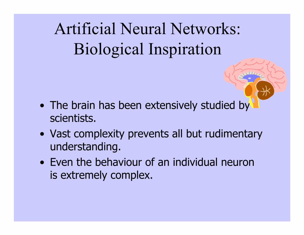
• The brain has been extensively studied byscientists.

• Vast complexity prevents all but rudimentaryunderstanding.

• Even the behaviour of an individual neuronis extremely complex.

Artificial Neural Networks:Biological Inspiration

Features of the Brain• >Ten billion (1010) neurons• Neuron switching time >10-3 secs• Face Recognition ~0.1 secs• On average, each neuron has several thousand

connections (to other neurons)• Hundreds of operations per second• Very high degree of parallel computation• Distributed representations (not all info in one spot)• Die off frequently (never replaced):

• redundancy & rewired

• Compensated for problems by massive parallelism

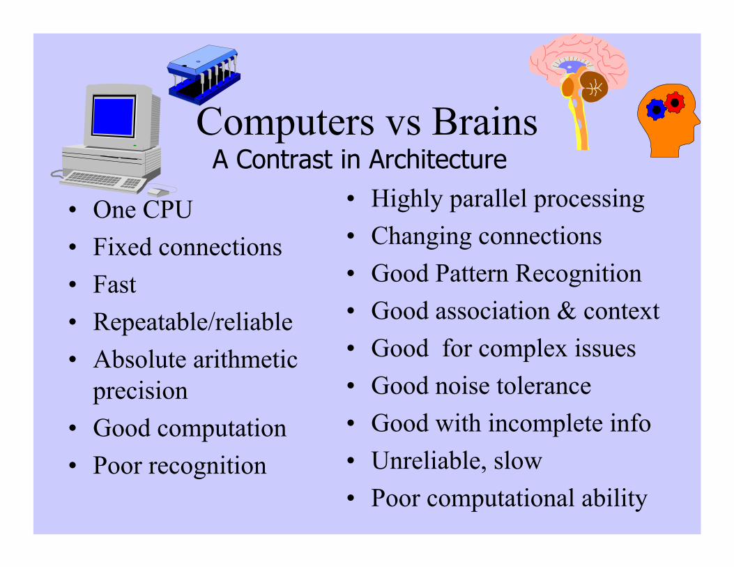
Computers vs Brains

• One CPU

• Fixed connections

• Fast

• Repeatable/reliable

• Absolute arithmeticprecision

• Good computation

• Poor recognition

• Highly parallel processing

• Changing connections

• Good Pattern Recognition

• Good association & context

• Good for complex issues

• Good noise tolerance

• Good with incomplete info

• Unreliable, slow

• Poor computational ability

A Contrast in Architecture

Why Artificial Neural Networks?

There are two basic reasons why we are interested in buildingartificial neural networks (ANNs):

• Technical viewpoint: Some problems such as character recognition or the prediction of future states of a system require massively parallel and adaptive processing.

• Biological viewpoint: ANNs can be used to replicate and simulate components of the human (or animal) brain, thereby giving us insight into natural information processing.

Why do we need another paradigm otherthan symbolic AI or Fuzzy logic for

building “intelligent” machines?

• Symbolic AI and Fuzzy logic are well-suited for representing explicit knowledge that can be appropriately formalized, or stated.

• However, learning in complex systems (e.g., biological) is mostly implicit – it is an adaptation process based on uncertain information by uncertain reasoning via experiences.

• Good in mechatronics for• Developing “unwritten” rules of operation and control.• Making a model or estimator of a system by observation.

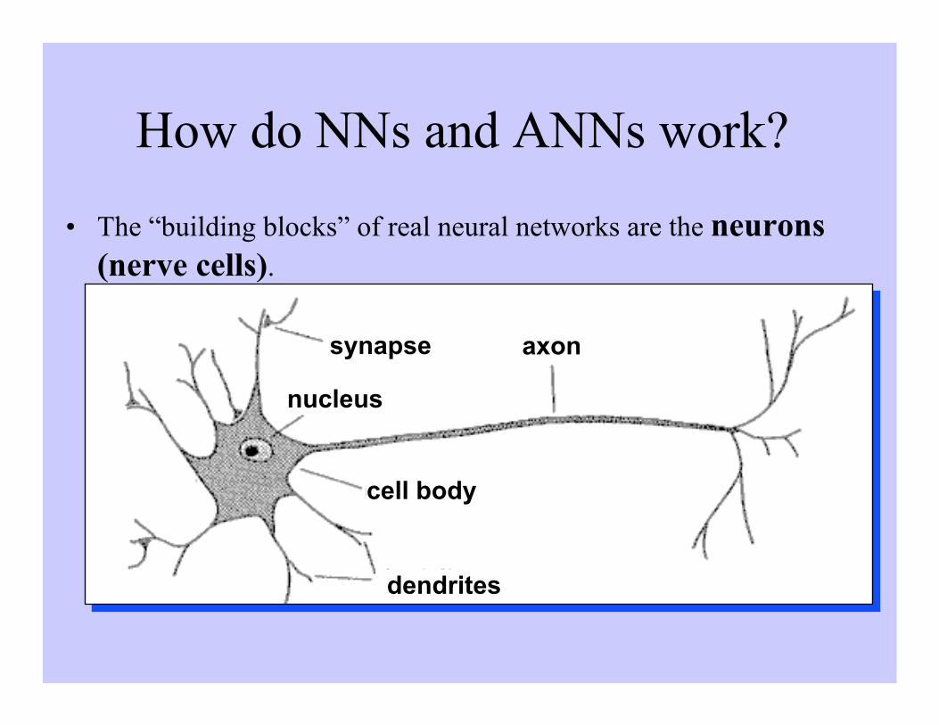
How do NNs and ANNs work?

• The “building blocks” of real neural networks are the neurons(nerve cells).

axon

cell body

synapse

nucleus

dendrites

axon

cell body

synapse

nucleus

dendrites

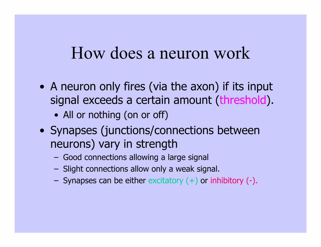
How does a neuron work

• A neuron only fires (via the axon) if its inputsignal exceeds a certain amount (threshold).• All or nothing (on or off)

• Synapses (junctions/connections betweenneurons) vary in strength– Good connections allowing a large signal– Slight connections allow only a weak signal.– Synapses can be either excitatory (+) or inhibitory (-).

How do they all piece together?

• Basically, each neuron• Transmits information as a series of electric impulses, so-

called spikes.• Receives inputs from many other neurons. One neuron can

be connected.• Changes its internal state (activation) based on all the current

inputs• Sends one output signal to many other neurons (>10,000 in

cases), possibly including itself (recurrent network).• Phase, frequency are also important in real neuron.

• In ANN we refer to neurons as units or nodes.

How do NNs (and ANNs) work?• In biological systems, neurons of similar functionality

are usually organized in separate areas (or layers).

• Often, there is a hierarchy of interconnected layerswith the lowest layer receiving sensory input andneurons in higher layers computing more complexfunctions.

• For example, neurons in a monkey’s visual cortex havebeen identified that are activated only when there is aface (monkey, human, or drawing) in the primate’svisual field.

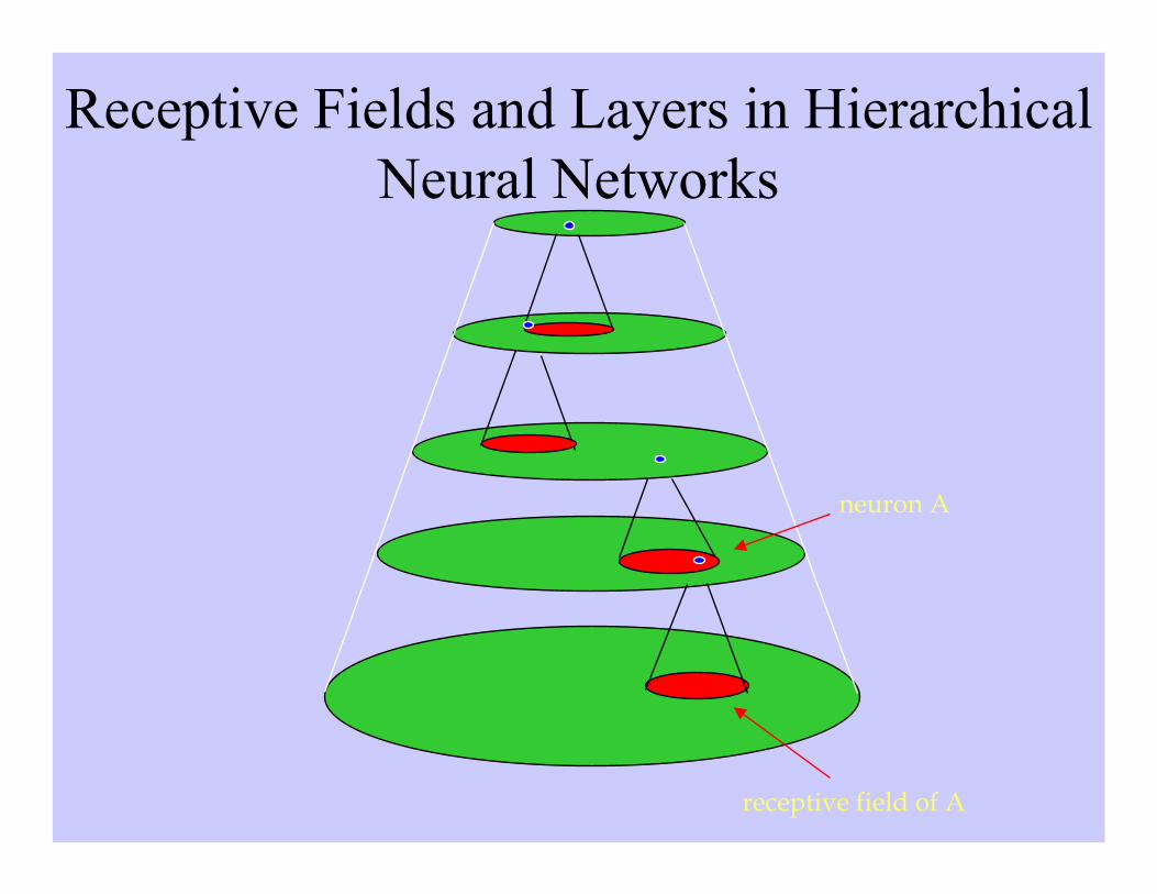
Receptive Fields and Layers in HierarchicalNeural Networks

neuron A

receptive field of A

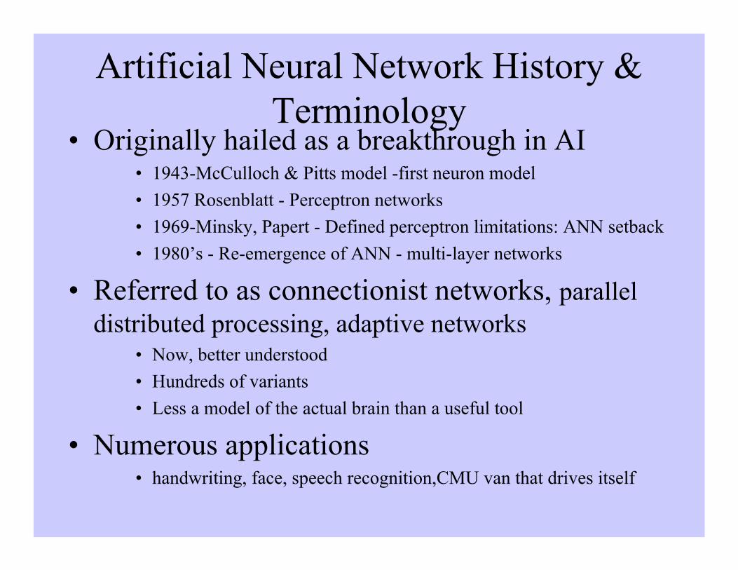
Artificial Neural Network History &Terminology

• Originally hailed as a breakthrough in AI• 1943-McCulloch & Pitts model -first neuron model

• 1957 Rosenblatt - Perceptron networks

• 1969-Minsky, Papert - Defined perceptron limitations: ANN setback

• 1980’s - Re-emergence of ANN - multi-layer networks

• Referred to as connectionist networks, paralleldistributed processing, adaptive networks

• Now, better understood

• Hundreds of variants

• Less a model of the actual brain than a useful tool

• Numerous applications• handwriting, face, speech recognition,CMU van that drives itself

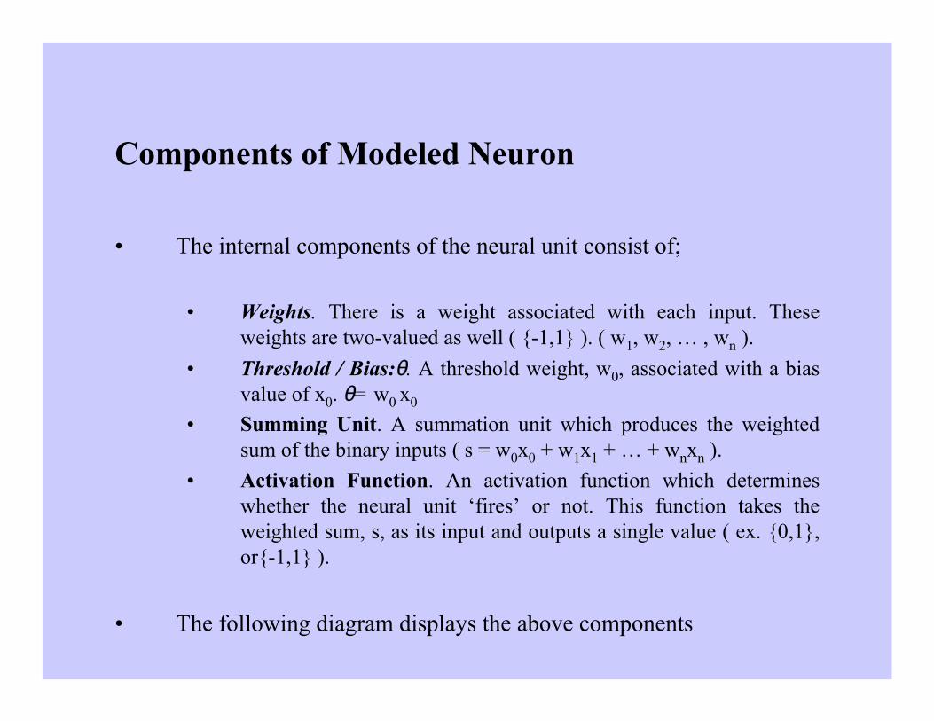
Components of Modeled Neuron

• The internal components of the neural unit consist of;

• Weights. There is a weight associated with each input. Theseweights are two-valued as well ( {-1,1} ). ( w1, w2, … , wn ).

• Threshold / Bias:θ. A threshold weight, w0, associated with a biasvalue of x0. θ= w0 x0

• Summing Unit. A summation unit which produces the weightedsum of the binary inputs ( s = w0x0 + w1x1 + … + wnxn ).

• Activation Function. An activation function which determineswhether the neural unit ‘fires’ or not. This function takes theweighted sum, s, as its input and outputs a single value ( ex. {0,1},or{-1,1} ).

• The following diagram displays the above components

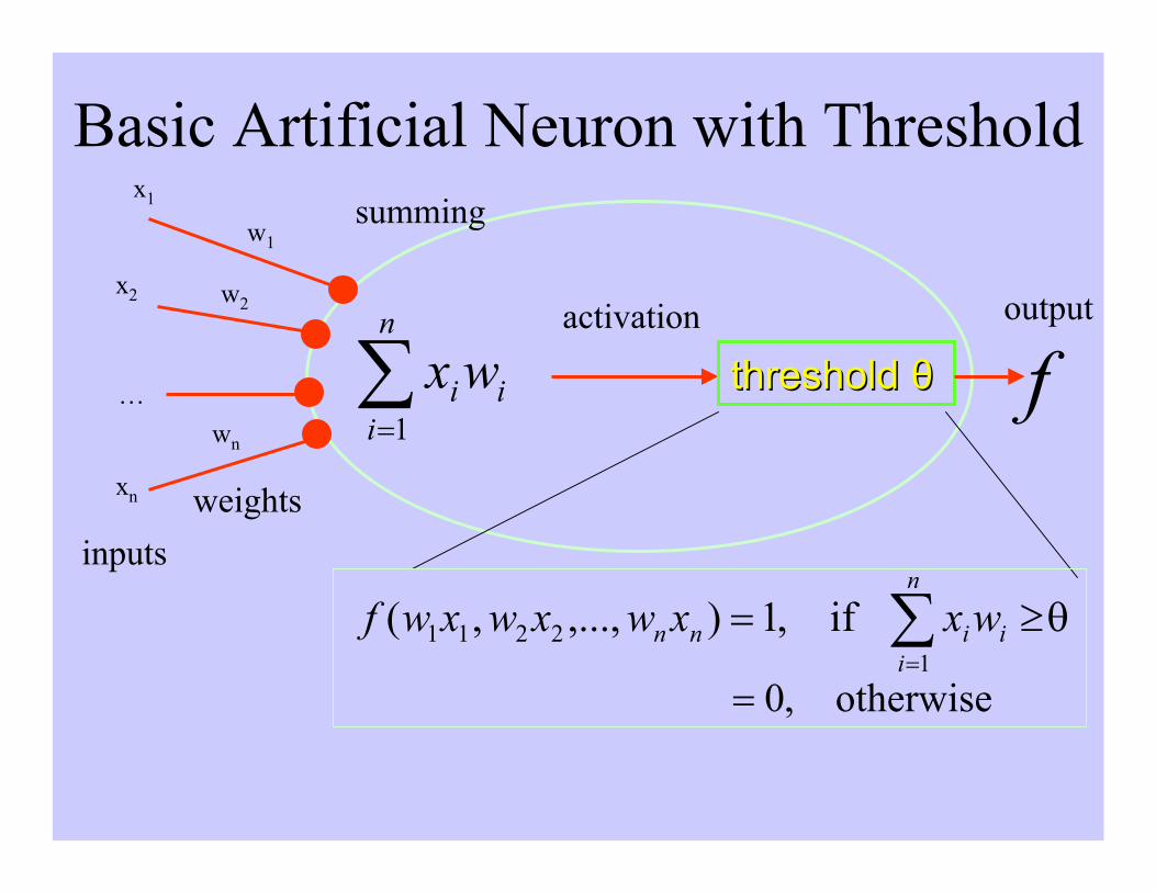
Basic Artificial Neuron with Threshold

threshold threshold θθ

x1

w1

x2 w2

wn

xn

… i

n

iiwx∑

=1

θ≥= ∑=

i

n

iinn wxxwxwxwf

12211 if,1),...,,(

otherwise,0=

activation output

inputs

f

summing

weights

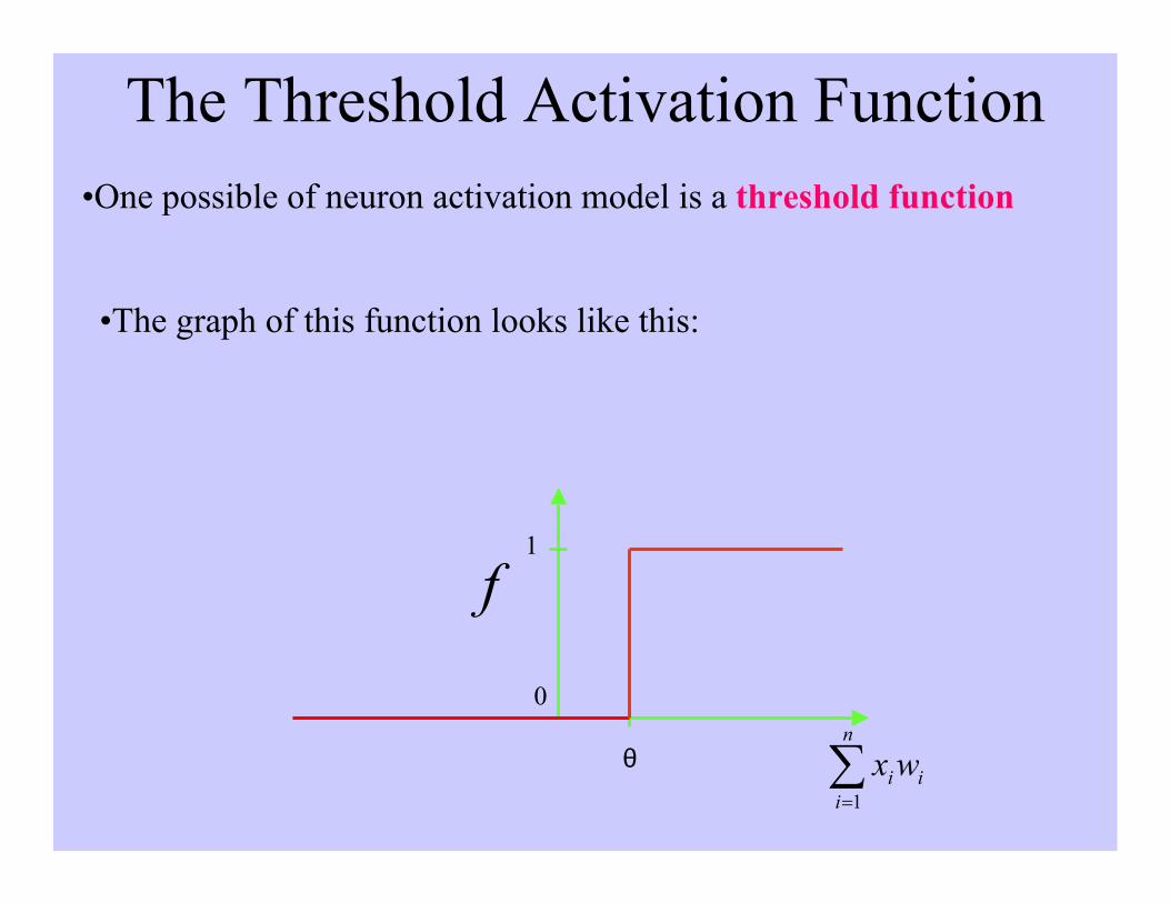
The Threshold Activation Function•One possible of neuron activation model is a threshold function

•The graph of this function looks like this:

1

0

θ

f

i

n

iiwx∑

=1

Properties of Artificial NeuralNets (ANNs)

• Many simple neuron-like threshold switching units

• Many weighted interconnections among units

• Highly parallel, distributed processing

• Learning is accomplished by tuning the connectionweights (wi) through training

• Training is usually separate from actual usage

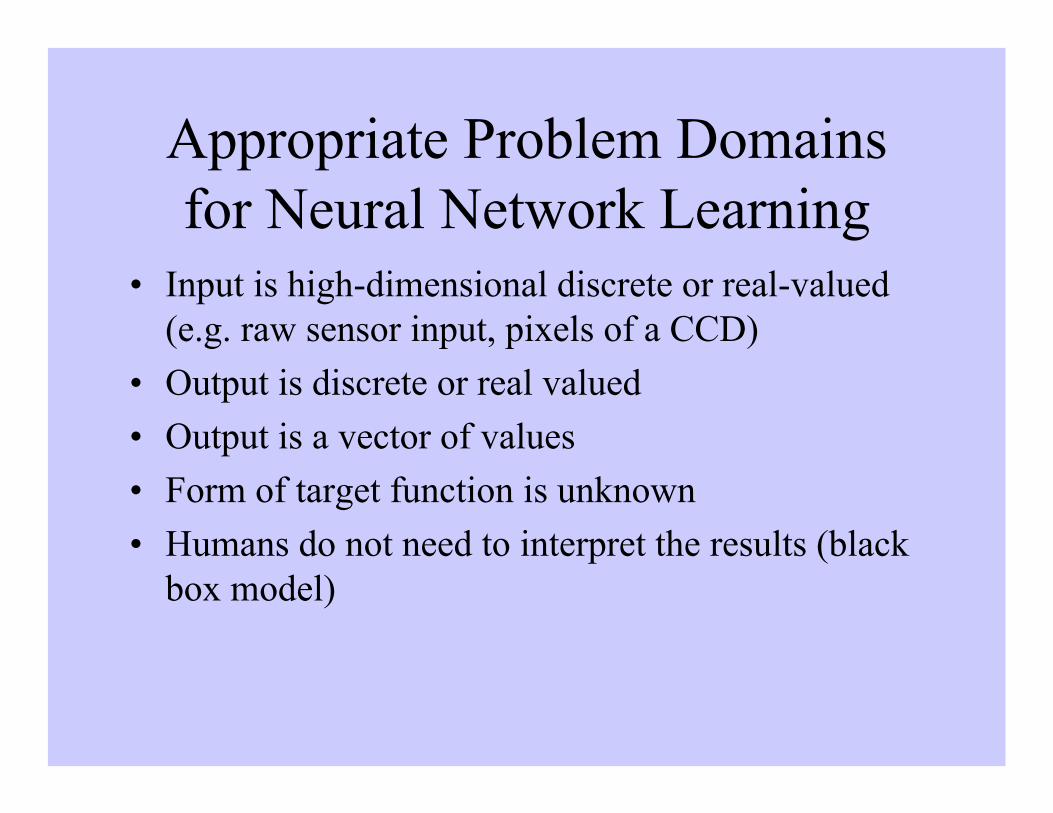
Appropriate Problem Domainsfor Neural Network Learning

• Input is high-dimensional discrete or real-valued(e.g. raw sensor input, pixels of a CCD)

• Output is discrete or real valued

• Output is a vector of values

• Form of target function is unknown

• Humans do not need to interpret the results (blackbox model)

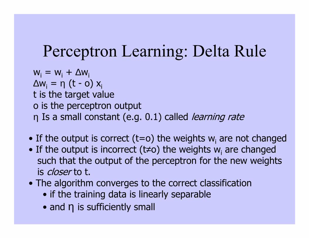
Perceptron Learning: Delta Rulewi = wi + ∆wi∆wi = η (t - o) xit is the target valueo is the perceptron outputη Is a small constant (e.g. 0.1) called learning rate

• If the output is correct (t=o) the weights wi are not changed• If the output is incorrect (t≠o) the weights wi are changed such that the output of the perceptron for the new weights is closer to t.• The algorithm converges to the correct classification

• if the training data is linearly separable• and η is sufficiently small

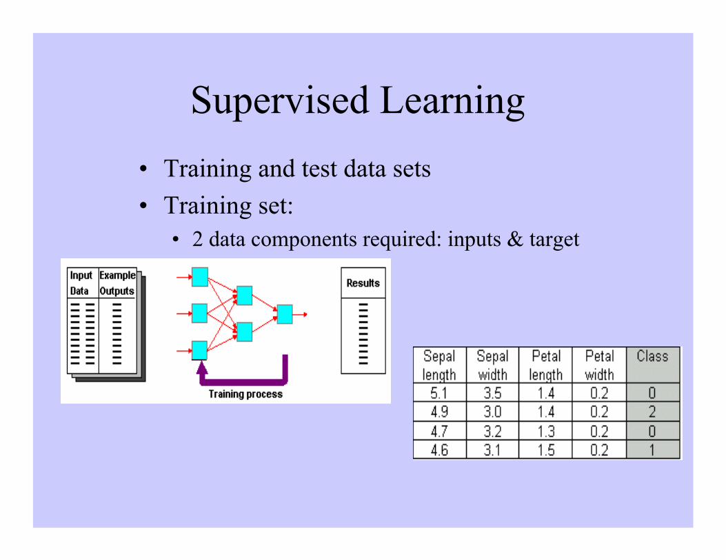
Supervised Learning

• Training and test data sets

• Training set:• 2 data components required: inputs & target

Perceptron Training

• Linear threshold is used.

• W - weight value

• t - threshold value

1 if Σ wi xi >tOutput= 0 otherwise{ i=0

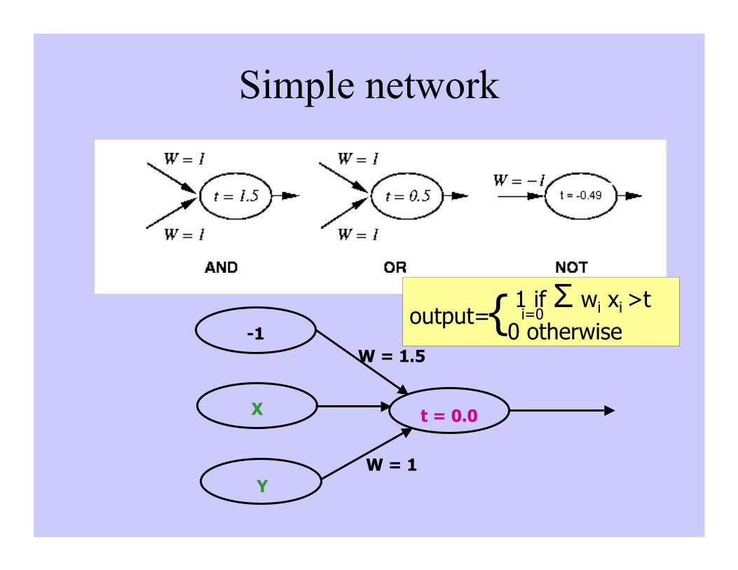
Simple network

t = 0.0

Y

X

W = 1.5

W = 1

-1

1 if Σ wi xi >toutput= 0 otherwise{ i=0

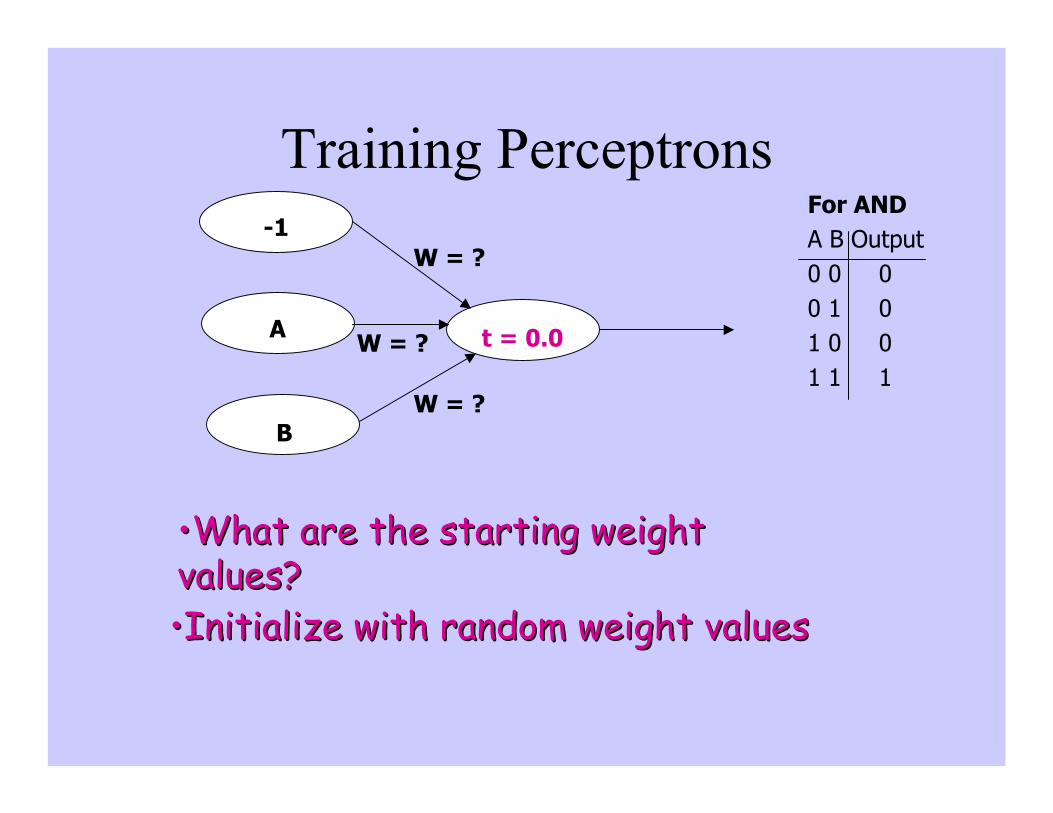
Training Perceptrons

t = 0.0

B

A

-1W = ?

W = ?

W = ?

For ANDA B Output0 0 00 1 01 0 01 1 1

••What are the starting weightWhat are the starting weightvalues?values?••Initialize with random weight valuesInitialize with random weight values

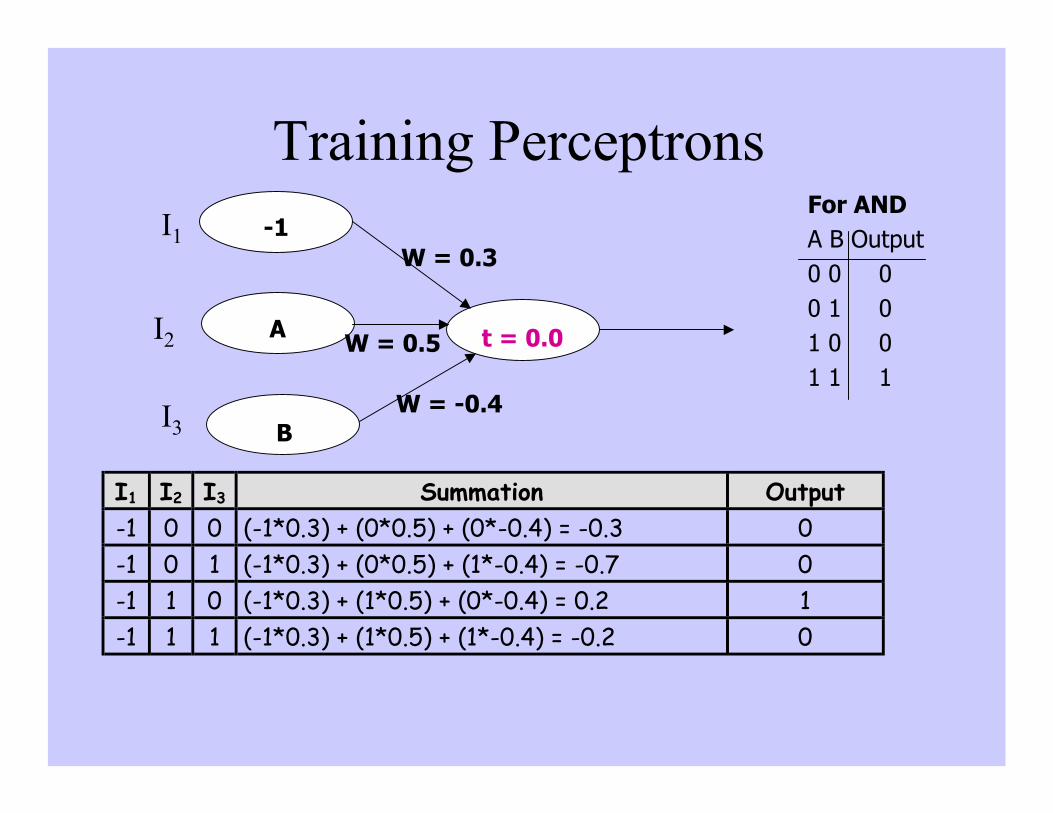
Training Perceptrons

t = 0.0

B

A

-1W = 0.3

W = -0.4

W = 0.5

I1 I2 I3 Summation Output-1 0 0 (-1*0.3) + (0*0.5) + (0*-0.4) = -0.3 0-1 0 1 (-1*0.3) + (0*0.5) + (1*-0.4) = -0.7 0-1 1 0 (-1*0.3) + (1*0.5) + (0*-0.4) = 0.2 1-1 1 1 (-1*0.3) + (1*0.5) + (1*-0.4) = -0.2 0

For ANDA B Output0 0 00 1 01 0 01 1 1

I1

I2

I3

Learning algorithmEpoch : Presentation of the entire training set to the neural

network.In the case of the AND function an epoch consistsof four sets of inputs being presented to thenetwork (i.e. [0,0], [0,1], [1,0], [1,1])

Error: The error value is the amount by which the valueoutput by the network differs from the targetvalue. For example, if we required the network tooutput 0 and it output a 1, then Error = -1

Learning algorithmTarget Value, T : When we are training a network we

not only present it with the input but also with avalue that we require the network to produce. Forexample, if we present the network with [1,1] forthe AND function the training value will be 1

Output , O : The output value from the neuron

Xi : Inputs being presented to the neuron

Wi : Weight from input neuron (Ij) to the output neuron

η: The learning rate. This dictates how quickly thenetwork converges. It is set by a matter ofexperimentation. It is typically 0.1

∆wi = η (T - o) xi

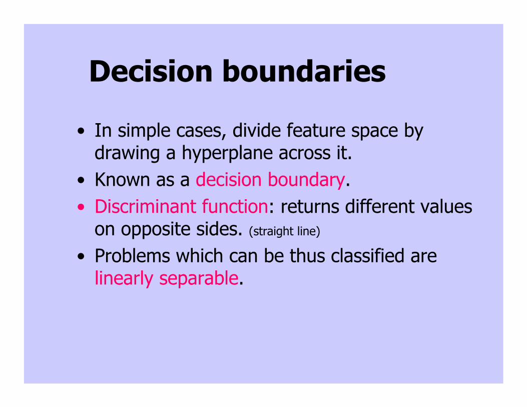
Decision boundaries

• In simple cases, divide feature space bydrawing a hyperplane across it.

• Known as a decision boundary.• Discriminant function: returns different values

on opposite sides. (straight line)

• Problems which can be thus classified arelinearly separable.

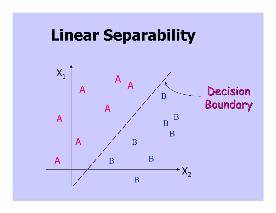
Linear Separability

X1

X2

A

B

A

A

AA

AA

B

B

B

BB

B

B DecisionDecisionBoundaryBoundary

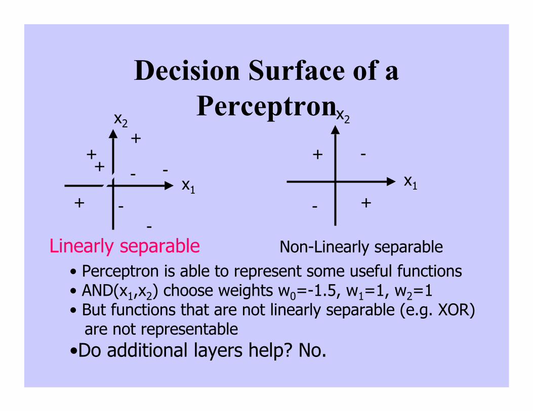
Decision Surface of aPerceptron

+

++

+ -

-

-

-x1

x2

+

+-

-

x1

x2

• Perceptron is able to represent some useful functions• AND(x1,x2) choose weights w0=-1.5, w1=1, w2=1• But functions that are not linearly separable (e.g. XOR) are not representable•Do additional layers help? No.

Linearly separable Non-Linearly separable

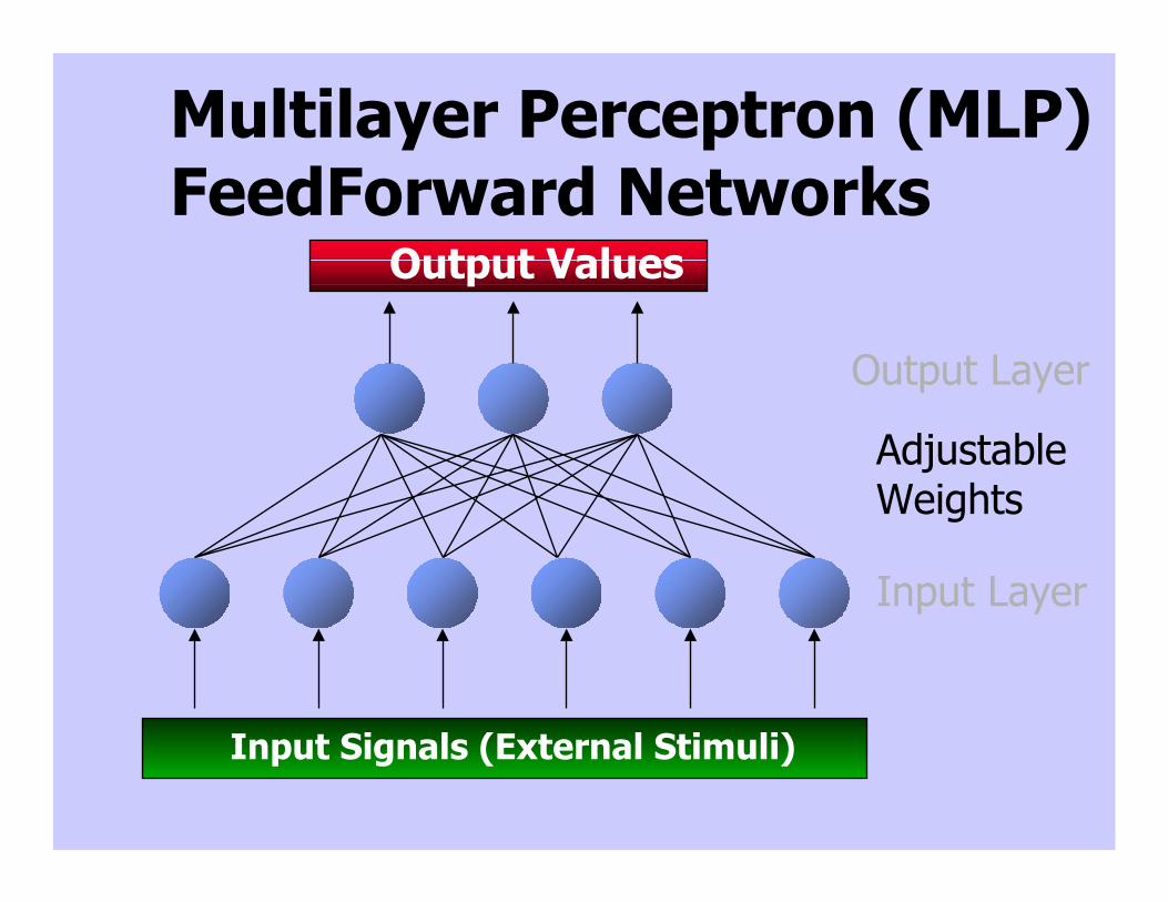
Multilayer Perceptron (MLP)FeedForward Networks

Output Values

Input Signals (External Stimuli)

Output Layer

AdjustableWeights

Input Layer

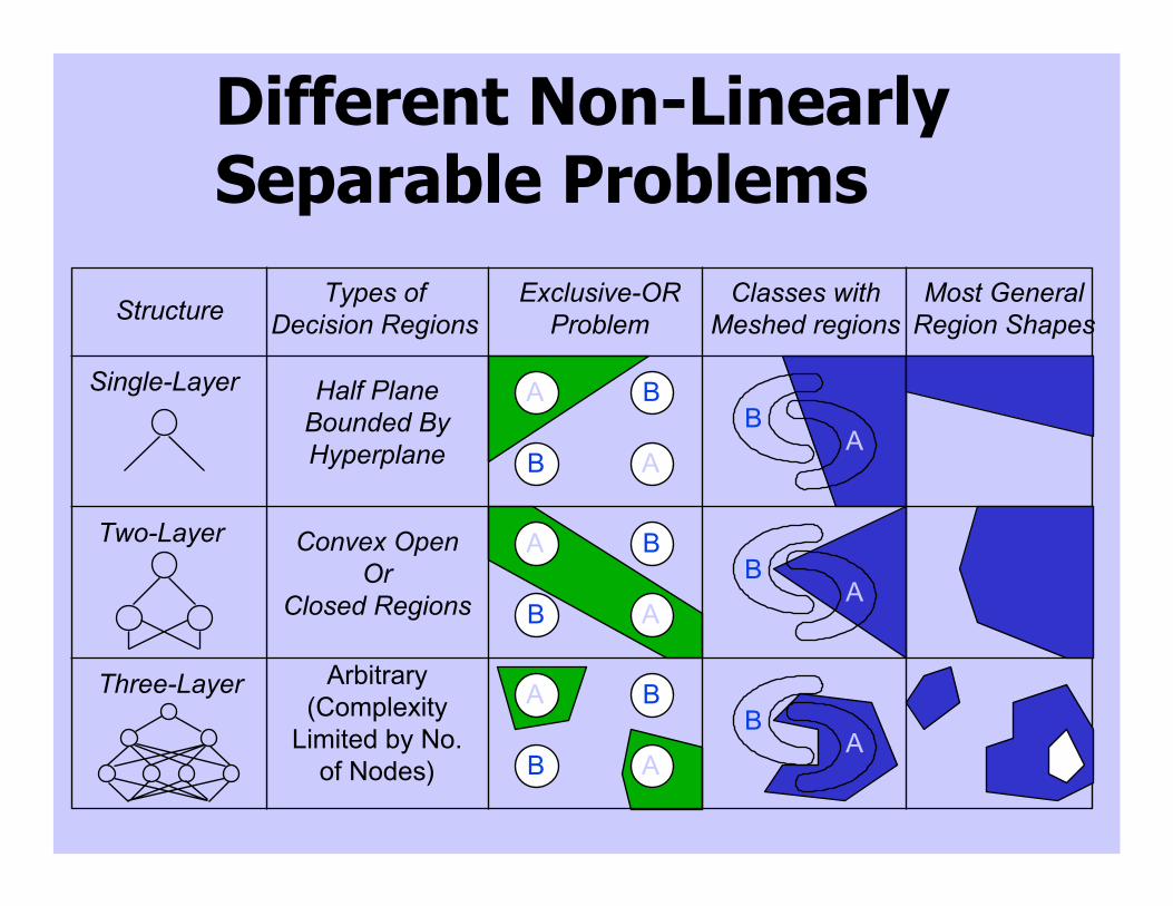
Different Non-LinearlySeparable Problems

StructureTypes of

Decision RegionsExclusive-OR

ProblemClasses with

Meshed regionsMost General

Region Shapes

Single-Layer

Two-Layer

Three-Layer

Half PlaneBounded ByHyperplane

Convex OpenOr

Closed Regions

Arbitrary(Complexity

Limited by No.of Nodes)

A

AB

B

A

AB

B

A

AB

B

BA

BA

BA

Types of Layers• The input layer.

– Introduces input values into the network.– No activation function or other processing.

• The hidden layer(s).– Perform classification of features– Two hidden layers are generally sufficient to solve

any problem– More solution details imply more layers may be better

• The output layer.– Functionally just like the hidden layers– Outputs are passed on to the world outside the neural

network (using weights).

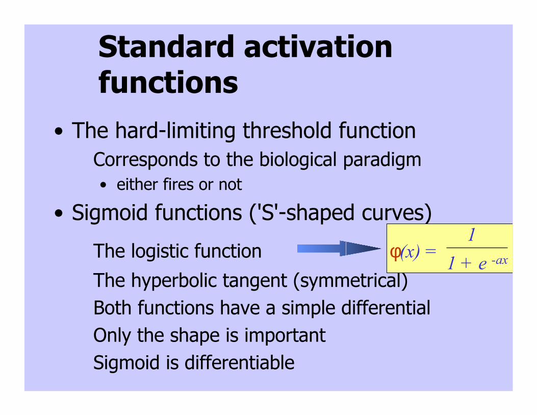
Standard activationfunctions

• The hard-limiting threshold function– Corresponds to the biological paradigm

• either fires or not

• Sigmoid functions ('S'-shaped curves)

– The logistic function– The hyperbolic tangent (symmetrical)– Both functions have a simple differential– Only the shape is important– Sigmoid is differentiable

φ(x) = 1

1 + e -ax

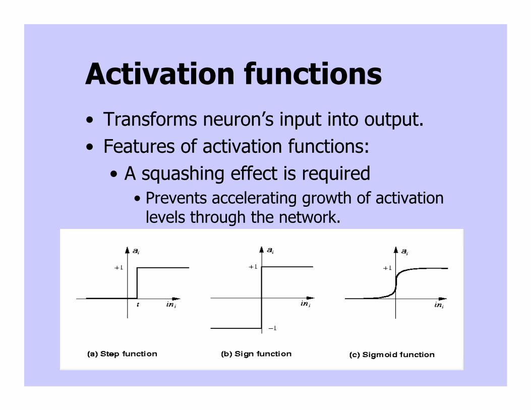
Activation functions• Transforms neuron’s input into output.• Features of activation functions:

• A squashing effect is required• Prevents accelerating growth of activation

levels through the network.

• Simple and easy to calculate

Standard activationfunctions

• The hard-limiting threshold function– Corresponds to the biological paradigm

• either fires or not

• Sigmoid functions ('S'-shaped curves)

– The logistic function– The hyperbolic tangent (symmetrical)– Both functions have a simple differential– Only the shape is important– Sigmoid is differentiable

φ(x) = 1

1 + e -ax

Training/Learning Algorithms

• Adjust neural network weights to map inputs tooutputs.

• Use a training set of sample patterns/data asbefore, where the desired output (given theinputs presented) is known.

• The purpose is to learn to generalize– Recognize features which are common to

good and bad examples

Back-Propagation

• A training procedure which allows multi-layerfeed-forward Neural Networks to be trained;

• Can theoretically perform “any” input-outputmapping;

• Can learn to solve linearly inseparable problems.

Activation functions andtraining

• For feed-forward networks:• A continuous function can be differentiated

allowing gradient-descent.• Back-propagation is an example of a

gradient-descent technique.• Reason for prevalence of sigmoid

Gradient Descent LearningRule

• Consider the linear sum unit without threshold andcontinuous output o (not just –1,1 or 0, 1)

o=w0 + w1 x1 + … + wn xn

• Train the wi’s such that they minimize the squarederror

E[w1,…,wn] = ½ Σd∈ D (td-od)2

where D is the set of training examples

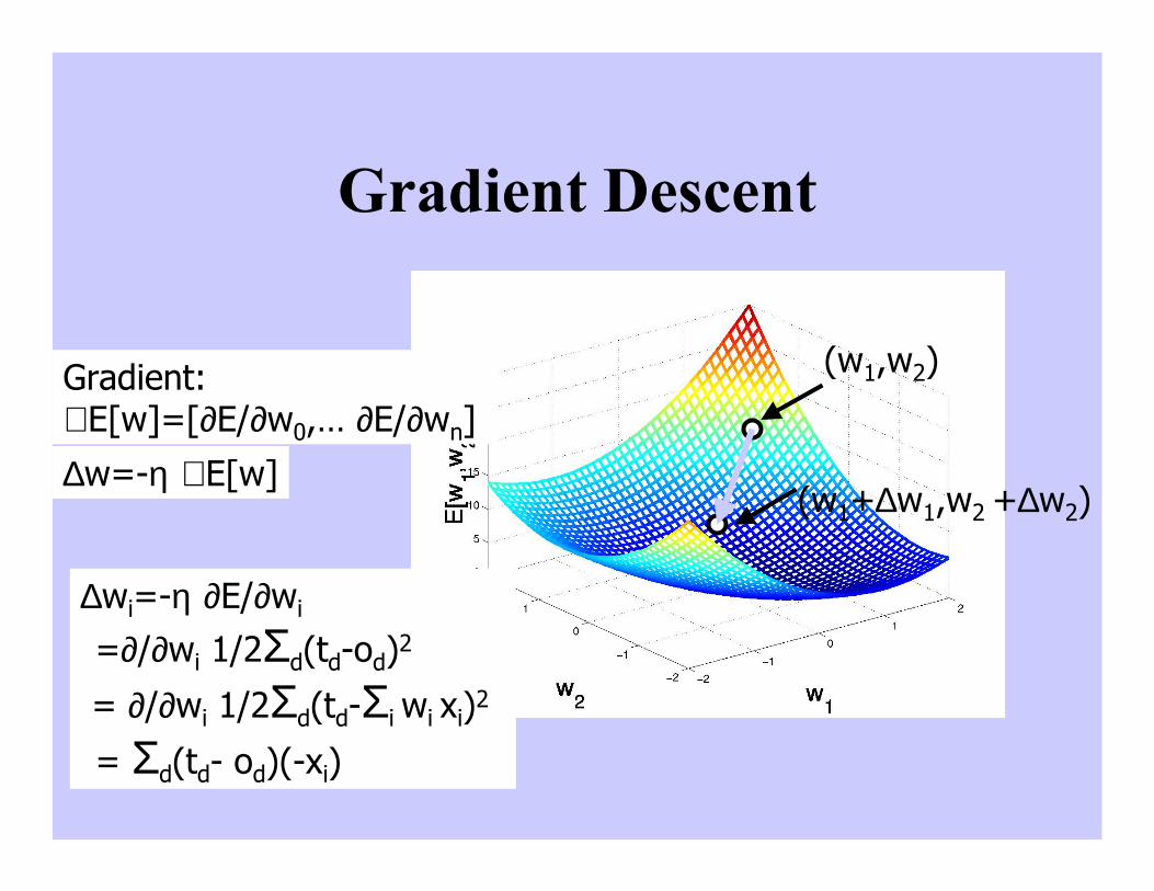
Gradient Descent

(w1,w2)

(w1+∆w1,w2 +∆w2)∆w=-η ∇ E[w]

∆wi=-η ∂E/∂wi

=∂/∂wi 1/2Σd(td-od)2

= ∂/∂wi 1/2Σd(td-Σi wi xi)2

= Σd(td- od)(-xi)

Gradient:∇ E[w]=[∂E/∂w0,… ∂E/∂wn]

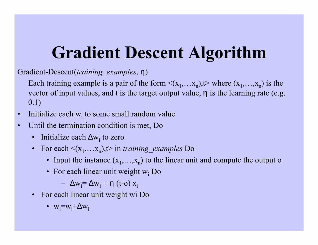
Gradient Descent AlgorithmGradient-Descent(training_examples, η)

Each training example is a pair of the form <(x1,…xn),t> where (x1,…,xn) is thevector of input values, and t is the target output value, η is the learning rate (e.g.0.1)

• Initialize each wi to some small random value

• Until the termination condition is met, Do

• Initialize each ∆wi to zero

• For each <(x1,…xn),t> in training_examples Do

• Input the instance (x1,…,xn) to the linear unit and compute the output o

• For each linear unit weight wi Do

– ∆wi= ∆wi + η (t-o) xi

• For each linear unit weight wi Do

• wi=wi+∆wi

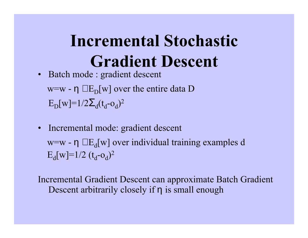
Incremental StochasticGradient Descent

• Batch mode : gradient descent

w=w - η ∇ ED[w] over the entire data D

ED[w]=1/2Σd(td-od)2

• Incremental mode: gradient descent

w=w - η ∇ Ed[w] over individual training examples d Ed[w]=1/2 (td-od)2

Incremental Gradient Descent can approximate Batch GradientDescent arbitrarily closely if η is small enough

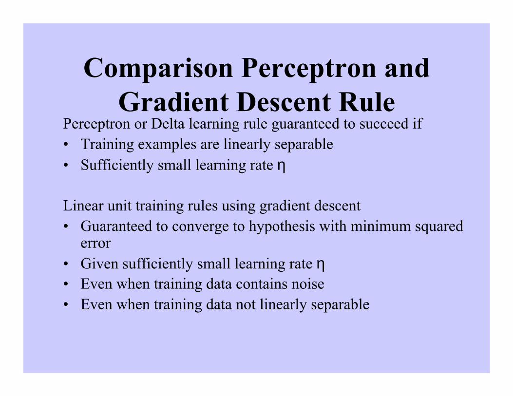
Comparison Perceptron andGradient Descent Rule

Perceptron or Delta learning rule guaranteed to succeed if• Training examples are linearly separable• Sufficiently small learning rate η

Linear unit training rules using gradient descent• Guaranteed to converge to hypothesis with minimum squared

error• Given sufficiently small learning rate η• Even when training data contains noise• Even when training data not linearly separable

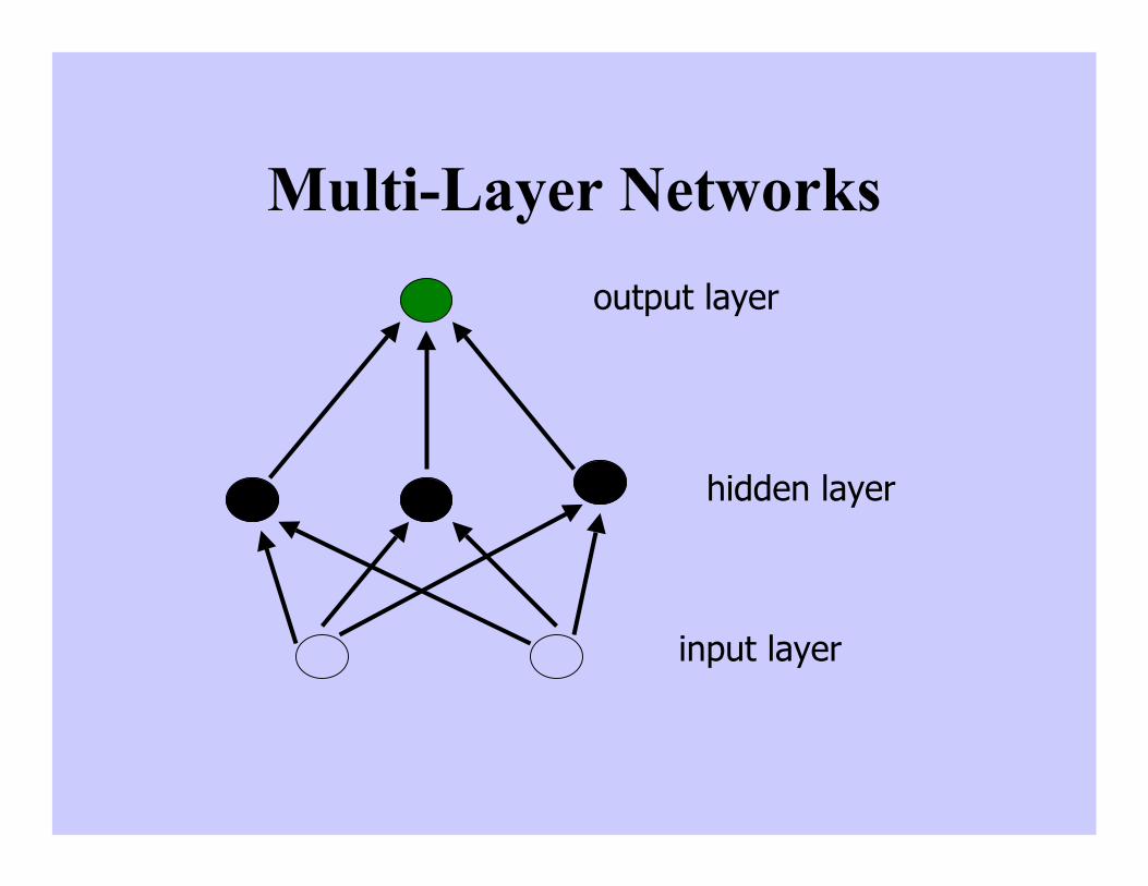
Multi-Layer Networks

input layer

hidden layer

output layer

Sigmoid Unit

Σ

x1

x2

xn

...

w1

w2

wn

w0

x0=1

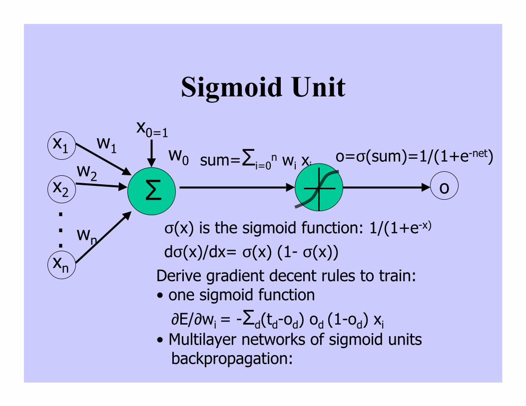
sum=Σi=0n wi xi

o

o=σ(sum)=1/(1+e-net)

σ(x) is the sigmoid function: 1/(1+e-x)

dσ(x)/dx= σ(x) (1- σ(x))Derive gradient decent rules to train:• one sigmoid function ∂E/∂wi = -Σd(td-od) od (1-od) xi• Multilayer networks of sigmoid units backpropagation:

Backpropagation Algorithm

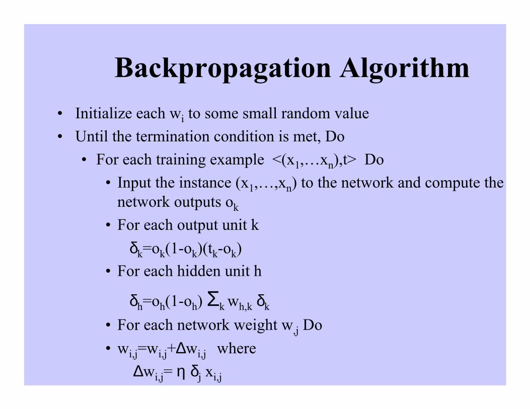
• Initialize each wi to some small random value

• Until the termination condition is met, Do

• For each training example <(x1,…xn),t> Do

• Input the instance (x1,…,xn) to the network and compute thenetwork outputs ok

• For each output unit k

δk=ok(1-ok)(tk-ok)

• For each hidden unit h

δh=oh(1-oh) Σk wh,k δk

• For each network weight w,j Do

• wi,j=wi,j+∆wi,j where

∆wi,j= η δj xi,j

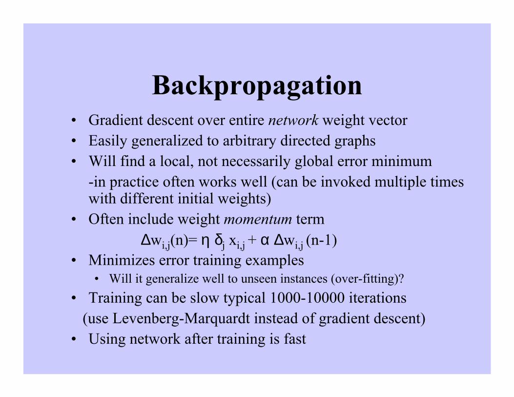
Backpropagation• Gradient descent over entire network weight vector• Easily generalized to arbitrary directed graphs• Will find a local, not necessarily global error minimum

-in practice often works well (can be invoked multiple timeswith different initial weights)

• Often include weight momentum term∆wi,j(n)= η δj xi,j + α ∆wi,j (n-1)

• Minimizes error training examples• Will it generalize well to unseen instances (over-fitting)?

• Training can be slow typical 1000-10000 iterations (use Levenberg-Marquardt instead of gradient descent)• Using network after training is fast

8 inputs 3 hidden 8 outputs

8-3-8 Binary Encoder-Decoder

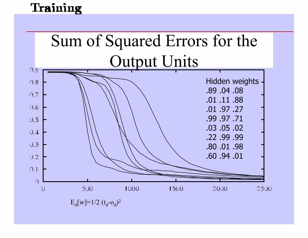
Hidden weights.89 .04 .08.01 .11 .88.01 .97 .27.99 .97 .71.03 .05 .02.22 .99 .99.80 .01 .98.60 .94 .01

Ed[w]=1/2 (td-od)2

Sum of Squared Errors for theOutput Units

Convergence of Backprop

Gradient descent to some local minimum• Perhaps not global minimum• Add momentum• Stochastic gradient descent• Train multiple nets with different initial weights

Nature of convergence• Initialize weights near zero• Therefore, initial networks near-linear• Increasingly non-linear functions possible as training

progresses

Applications• The properties of neural networks define where

they are useful.– Can learn complex mappings from inputs to outputs,

based solely on samples.– Difficult to analyse: firm predictions about neural

network behaviour difficult;• Questionable for safety-critical applications.

– Require limited understanding from trainer, who canbe guided by heuristics.

– Defined operational area: ANNs cannot extrapolate.Training sets bounds model accuracy.

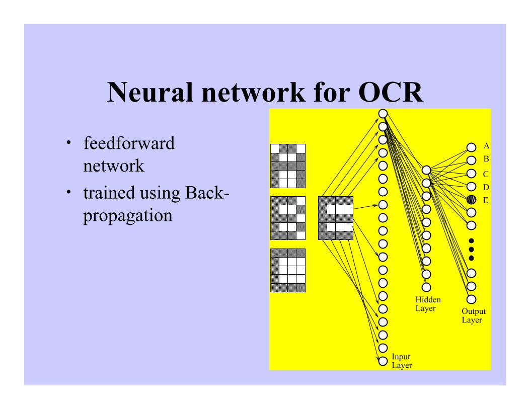
Neural network for OCR

• feedforwardnetwork

• trained using Back-propagation

��

��

��

��

��

��

��

��

��

��

��

��

��

��

��

��

��

��

��

��

��

��

��

��

��

��

��

��

��

��

��

��

��

��

��

��

��

��

��

��

��

��

��

��

��

��

��

��

��

��

A

B

E

D

C

Output Layer

Input Layer

Hidden Layer

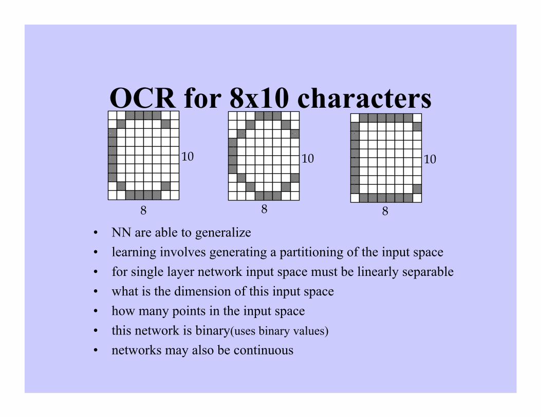
OCR for 8x10 characters

• NN are able to generalize

• learning involves generating a partitioning of the input space

• for single layer network input space must be linearly separable

• what is the dimension of this input space?

• how many points in the input space?

• this network is binary(uses binary values)

• networks may also be continuous

��

��

��

��

��

��

��

��

��

��

��

��

��

��

��

��

��

��

��

��

��

��

��

��

��

��

��

��

��

��

��

��

��

��

��

��

��

��

��

��

��

��

��

��

��

��

��

��

��

��

8

10

8 8

1010

Engine management

• The behaviour of a car engine is influencedby a large number of parameters– temperature at various points– fuel/air mixture– lubricant viscosity.

• Major companies have used neural networksto dynamically tune an engine depending oncurrent settings.

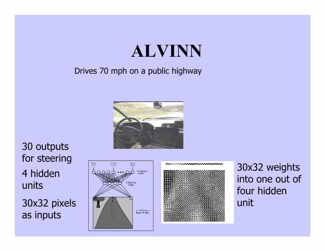
ALVINNDrives 70 mph on a public highway

30x32 pixelsas inputs

30 outputsfor steering4 hiddenunits

30x32 weightsinto one out offour hiddenunit

Signature recognition

• Each person's signature is different.• There are structural similarities which are

difficult to quantify.• One company has manufactured a machine

which recognizes signatures to within a highlevel of accuracy.– Considers speed in addition to gross shape.– Makes forgery even more difficult.

Sonar target recognition

• Distinguish mines from rocks on sea-bed• The neural network is provided with a large

number of parameters which are extractedfrom the sonar signal.

• The training set consists of sets of signalsfrom rocks and mines.

Stock market prediction

• “Technical trading” refers to trading basedsolely on known statistical parameters; e.g.previous price

• Neural networks have been used to attemptto predict changes in prices.

• Difficult to assess success since companiesusing these techniques are reluctant todisclose information.

Mortgage assessment

• Assess risk of lending to an individual.• Difficult to decide on marginal cases.• Neural networks have been trained to make

decisions, based upon the opinions of expertunderwriters.

• Neural network produced a 12% reduction indelinquencies compared with human experts.

Neural NetworkProblems

• Many Parameters to be set• Overfitting• long training times• ...

Parameter setting

• Number of layers• Number of neurons

• too many neurons, require more training time

• Learning rate• from experience, value should be small ~0.1

• Momentum term• ..

Over-fitting

• With sufficient nodes can classify anytraining set exactly

• May have poor generalization ability.• Cross-validation with some patterns

– Typically 30% of training patterns– Validation set error is checked each epoch– Stop training if validation error goes up

Training time

• How many epochs of training?– Stop if the error fails to improve (has reached a

minimum)– Stop if the rate of improvement drops below a

certain level– Stop if the error reaches an acceptable level– Stop when a certain number of epochs have

passed

Caution:

• When you have a new hammereverything tends to be a nail.

Introduction to Artificial Neural Networks - Faculty Web...

Documents

Transcript of Introduction to Artificial Neural Networks - Faculty Web...