Introduction to AR models

Introduction to AR models In an autoregressive model, the regression technique is used to formulate a time series problem. In order to implement autoregressive models, we forecast the future observations using a linear combination of past observations of the same variable i.e. to predict y⌃t which is the future forecast of a variable, we need one or more past observations of yt that is yt-1, yt-2, etc. But to implement these techniques, we need to abide by some assumptions. There are two fundamental assumptions to build an autoregressive model. They are -

1. Stationarity 2. Autocorrelation

Let us understand both these assumptions one by one. We will also learn how to make a non-stationary time series into a stationary one so as to use the autoregressive models.

Stationarity

If a time series is stationary, its statistical properties like mean, variance, and covariance will be the same throughout the series, irrespective of the time at which you observe them. As the series will be stationary, the statistical properties such as mean, variance and covariance need to be the same and thus these need to be followed by a series with temporal data also.

The following image illustrates a stationary time series in which the properties such as mean, variance and covariance are the same for any two-time windows.

© Copyright 2020. UpGrad Education Pvt. Ltd. All rights reserved

https://www.investopedia.com/terms/c/covariance.asp

Let us understand now what is white noise. White Noise is an example of a stationary time series with purely random, uncorrelated observations with no identifiable trend, seasonal or cyclical components. A white noise series can seen from the image below


Notice that there are no identifiable trends, seasonal or cyclical components. So a white noise series is basically an example of a stationary series. The following example of a non-stationary series is called random walk.

A random walk is a time series where the current observation is equal to the previous observation plus a random change. Here, variance increases over time resulting in a non-stationary series. In general, a stationary time series will have no long-term predictable patterns such as trends or seasonality. Time plots will show the series to roughly have a horizontal trend with constant variance.


Stationarity Tests Most of the time, visually, you can see that the series has a clear trend or seasonal component to comment about its stationarity. However, you cannot say that for sure as you also have to test whether its statistical properties, such as mean, variance etc. remain constant. This is not possible to comment by inspecting the time series visually. There are some formal tests for checking this.

There are two formal tests for stationarity based on hypothesis testing. The unit root test is a common procedure to determine whether a time series is stationary or not. If the existence of a unit root for a series cannot be rejected, then the series is said to be non-stationary.

Kwiatkowski-Phillips-Schmidt-Shin (KPSS) Test

● Null Hypothesis (H0): The series is stationary ○ p−value>0.05

● Alternate Hypothesis (H1): The series is not stationary ○ p−value≤0.05

Augmented Dickey-Fuller (ADF) Test

● Null Hypothesis (H0): The series is not stationary ○ p−value>0.05

● Alternate Hypothesis (H1): The series is stationary ○ p−value≤0.05

Interpretation of p-value.

A p-value below a threshold (such as 5% or 1%) suggests we reject the null hypothesis, otherwise, a p-value above the threshold suggests we fail to reject the null hypothesis.

● p−value>0.05: Fail to reject the null hypothesis (H0). ● p−value≤0.05: Reject the null hypothesis (H0).


For the airline passenger traffic example, we need to first check whether the series is stationary or not. We can do that visually inspecting and checking if we can see from the graph ourselves.

Later, we apply the Augmented Dickey-Fuller (ADF) Test and the Kwiatkowski-Phillips-Schmidt-Shin (KPSS) Test as shown in the images below.

On inspecting the ADF test, we know that as per the null hypothesis, the series is not stationary When p−value>0.05. Thus, we know that the time series in the airline passenger data is not a stationary time series and we need to make it stationary first by making the variance and the mean constant.


This is done by the Box-Cox transformation and the Differencing over the time series and will be explained in the sections below.

Converting a Non-Stationary Time-Series to a Stationary Time-Series

For implementing the auto-regressivce models, we discussed that the time-series needs to be stationary. And thus, for a non-stationary time series, we need to first convert it into a stationary one. There are two tools to convert a non-stationary series into stationary series are as follows:

1. Differencing 2. Transformation

To remove the trend (to make the mean constant) in a time series you use the technique called differencing. As the name suggests, in differencing you compute the differences between consecutive observations. It’s just like differencing a sloped line so as to make the slope zero. Differencing stabilises the mean of a time series by removing changes in the level of a time series and therefore eliminating (or reducing) trend and seasonality.

For Example:

Original time series After 1st order differencing After 2nd order differencing

50

180 130

420 240 110

770 350 110

1240 470 120

1820 580 110

Here 1st order differencing is calculated by the difference of two consecutive observations of the original time series. 2nd order differencing is calculated by the difference of two consecutive observations of the 1st order differenced series. This is similar to the difference in the y values


divided by the x values while calculating a slope of a line. You can observe the effect of differencing on an original time series shown in the first image below, and how after the second order differencing, the time series looks like.

At the first difference level, it still has a linear trend but we have successfully removed the higher-order trend observed in the original time series. After the 2nd difference level, the series obtained is mostly a horizontal line. There is no overall visible trend in this series and thus you can say the series obtained is a stationary series.

The other method to introduce the stationarity is making the variance constant. There can be many transformation methods used to make a non-stationary series stationary but here, we are discussing the Box-Cox transformation.


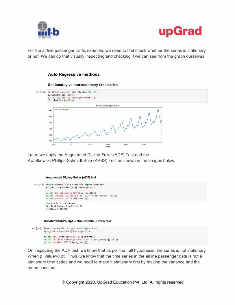
The mathematical formulae that Box-cox transformation is:

where y is the original time series and y(λ) is the transformed series. The procedure for the Box-Cox transformation is to find the optimal value of λ between -5 and 5 that minimizes the variance of the transformed data.


Now, applying the box-cox transformation and differencing the airline passenger dataset in python, we get the following:

In the above image, you can clearly see that the variance in the magnitude of the time series values as the series progresses is fairly constant. Thus the box-cox transformation is applied successfully.


Also, the trend in the time series gets removed after the series is differenced using the above steps.

ACF and PACF

Autocorrelation is capturing the relationship between observations yt at time t and yt-k at time k time period before t. In simpler words, autocorrelation helps us to know how a variable is influenced by its own lagged values. We looked at two Autocorrelation measures here:

1. Autocorrelation function (ACF) 2. Partial autocorrelation function (PACF)

The autocorrelation function tells about the correlation between an observation with its lagged values. It helps you to determine which lag of the observation is influencing it the most.


In the above example, we see the time series with lag 1 and lag 2 of its original time series. Now let’s see the autocorrelation plot of the same data.

Here, we clearly see that the current observation is significantly correlated with lag 1 and lag 2. The other interesting thing to notice is that the autocorrelation function captures both direct and indirect relationships between the variables. For example:


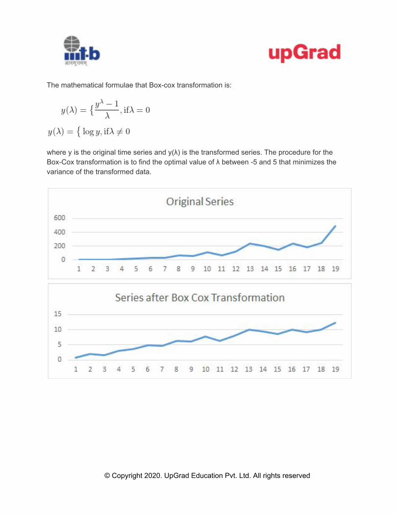
An ACF plot shown in an example taken by the SME is shown below

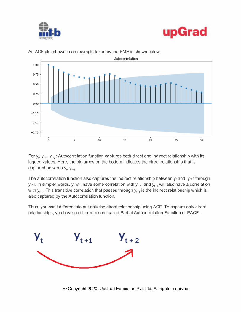
For yt, yt+1, yt+2: Autocorrelation function captures both direct and indirect relationship with its lagged values. Here, the big arrow on the bottom indicates the direct relationship that is captured between yt, yt+2

The autocorrelation function also captures the indirect relationship between yt and yt+2 through yt+1. In simpler words, yt will have some correlation with yt+1, and yt+1 will also have a correlation with yt+2. This transitive correlation that passes through yt+1 is the indirect relationship which is also captured by the Autocorrelation function.

Thus, you can’t differentiate out only the direct relationship using ACF. To capture only direct relationships, you have another measure called Partial Autocorrelation Function or PACF.


A PACF plot shown in an example taken by the SME is shown below

For the airline passenger traffic dataset, the ACF and the PACF plots can be plotted in python as shown below.

In the ACF plot above, you can see the plot for 30 lags in the dataset. We decide the window size, that is q using the above plot. As you can see, the highest lag after which the autocorrelation dies down is 1. Thus q =1 will be suitable for the airline passenger problem.


In the PACF plot above, the highest lag for which the partial autocorrelation is significantly high is the p = 1. Thus this value of p will be suitable while using the ARIMA techniques in the airline passenger problem. We performed the box cox transformation on the entire dataset and not just the train data. Thus, before starting with the models, we need to split the box cox data into train and test and that is shown below.


The Simple Auto Regressive Model (AR)

The Simple Auto Regressive model predicts the future observation as linear regression of one or more past observations. In simpler terms, the simple autoregressive model forecasts the dependent variable (future observation) when one or more independent variables are known (past observations). This model has a parameter ‘p’ called lag order. Lag order is the maximum number of lags used to build ‘p’ number of past data points to predict future data points.

Example: Consider an example of forecasting monthly sales of ice cream for the year 2021 on the basis of the previous 3 years' monthly sales data of the ice cream. This can be one of the simple autoregressive models.

To determine the value of parameter ‘p’.

● Plot partial autocorrelation function

● Select p as the highest lag where partial autocorrelation is significantly high

Here, the lag value of 1, 2, 4 and 12 has a significant level of confidence. i.e., significant level of influence on future observation (refer to the red line). Hence, the value of 'p' will be set to 12 since that is the highest lag where partial autocorrelation is significantly high.

● Build autoregression model equation:


The past values which have a significant value are 1, 2, 4 and 12. Therefore, in the regression model the independent variables yt-1, yt-2, yt-4 and yt-12 which are the observations from the past have been taken to predict the dependent variable y⌃t.

Now let us get back again to the airline passenger dataset and build an AR model on it. In order to build the AR model, the stationary series is divided into train and test data.

The following steps are performed on the airline passenger data to build the AR model. The forecast plot is then calculated along with the MAPE value and compared with the previously built models.


Moving Average Model (MA)

The Moving Average Model models the future forecasts using past forecast errors in a regression-like model. This model has a parameter ‘q’ called window size over which linear combination of errors are calculated.

Example: Forecast daily ice cream sales for the next 5 days when on an average daily ice cream sale is 30.


Explanation: On the first day you predicted the sale to be the average sale that is 30 but actual demand came to be around 27. There is an error of -3. For the next day, you predicted the sale of ice cream to be mean along with a percentage of error of previous day prediction. i.e., 30+0.5(-3) = 28.5. Similarly, you calculate the forecast for the rest of the days. The prediction of sales of ice cream is moving around the overall mean 30. For this reason, the model is called the moving average (MA) model. We can look at the following plot to confirm this.

Now, in order to build the moving average model, you need to determine the value of parameter ‘q’. Let's follow the steps below to do that.

● Plot the Autocorrelation function (ACF)


● Select q as the highest lag beyond which autocorrelation dies down:

Here, for lag 1 and lag 2 the autocorrelation is above significance level. Select q=2 as it is the highest lag beyond which autocorrelation dies down.

● Build Moving Average model equations as:

The following steps are performed on the airline passenger data to build the MA model. The forecast plot is then calculated along with the MAPE value and compared with the previously built models.


Auto Regressive Moving Average (ARMA) A time series that exhibits the characteristics of an AR(p) and/or an MA(q) process can be modelled using an ARMA(p,q) model.

ARMA (1,1) equation: For p = 1 and q=1 —

Here, ^y is the forecasted value.


To determine the parameters ‘p’ and ‘q’ —

● Plot autocorrelation function (ACF) and partial autocorrelation function (PACF)

● If you check the plot for PACF, you will see that you need to select p = 1 as the highest lag where partial autocorrelation is significantly high.

● Similarly from the ACF plot, select q = 2 as the highest lag beyond which autocorrelation dies down.

● So, we would select an ARMA (1, 2) model in this example.


The following steps are performed on the airline passenger data to build the ARMA model. The forecast plot is then calculated along with the MAPE value and compared with the previously built models.


Auto Regressive Integrated Moving Average (ARIMA)

Steps of ARIMA model

● Original time series is differenced to make it stationary ● Differenced series is modeled as a linear regression of

○ One or more past observations ○ Past forecast errors

● ARIMA model has three parameters ○ p: Highest lag included in the regression model ○ d: Degree of differencing to make the series stationary ○ q: Number of past error terms included in the regression model ○ Here the new parameter introduced is the ‘I’ part called integrated. It removes the

trend (non-stationarity) and later integrates the trend to the original series.

So if you think about it, ARIMA is nothing different from what you have done so far. Initially you applied both the box cox transformation and differencing in order to convert the data into a stationary time-series data. Here, you are just applying box cox before building the model and letting the model take care of the differencing i.e. the trend component itself.


Let's now quickly revisit the equations.

ARIMA(1,1,1) Equations:

Here, Zt is the first order differencing for time series.

To determine the parameters ‘p’, ‘d’ and ‘q’

● For ‘d’: Select d as the order of difference required to make the original time series stationary. We can verify if this differenced series is stationary or not by using the stationarity tests: ADF or KPSS test.

● For ‘p’ and ‘q’: Plot ACF and PACF of the 1st order differenced time series. Find the value of ‘p’ and ‘q’ as discussed previously with the earlier Auto Regressive Models.

● The last step in the ARIMA model is to recover the original time series forecast.


The following steps are performed on the airline passenger data to build the ARIMA model. The forecast plot is then calculated along with the MAPE value and compared with the previously built models.


Seasonal Auto Regressive Integrated Moving Average (SARIMA) SARIMA brings all the features of an ARIMA model with an extra feature - seasonality.

The non-seasonal elements of SARIMA

● Time series is differenced to make it stationary. ● Models future observation as linear regression of past observations and past forecast

errors.

The seasonal elements of SARIMA

● Perform seasonal differencing on time series. ● Model future seasonality as linear regression of past observations of seasonality and

past forecast errors of seasonality.

Example:

To forecast quarterly ice cream sales of 2020 using the Quarterly ice cream sales data for the last 4 years.


Explanation:

● Historical Sales follow a quarterly seasonality and in four years we get 16 data points. ● Future sales is related to past sales with lag = 4 ● Sales over the last 4 years is steadily increasing

The above three points make clear that this example has a seasonal component.

The parameters ‘p’, ‘d’, ‘q’ and ‘P’, ‘D’, ‘Q’:

● Non-seasonal elements ○ p: Trend autoregression order ○ d: Trend difference order ○ q: Trend moving average order

● Seasonal elements ○ m: The number of time steps for a single seasonal period ○ P: Seasonal autoregressive order ○ D: Seasonal difference order ○ Q: Seasonal moving average order


Equation for SARIMA(1,0,0)(0,1,1)4:

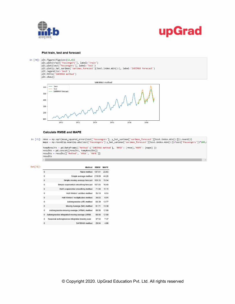
The following steps are performed on the airline passenger data to build the SARIMA model. The forecast plot is then calculated along with the MAPE value and compared with the previously built models.


SARIMAX

SARIMAX has three components:

● Non-seasonal elements ○ Models future observation as a linear regression of past observations and past

forecast errors. ○ Performs differencing to make time-series stationary.

● Seasonal elements ○ Models seasonality as the linear regression of past observations and past

forecast errors from previous seasons. ○ Perform seasonal differencing to make time-series stationary over seasons.

● Exogenous variable ○ Models future observations as linear regression of an external variable.

Example: Forecast quarterly ice cream sales for 2020 when you have the data of quarterly sales of the ice cream for the last 4 years.

In the above time plot, sales data displays trend and seasonality but peaks are not periodic. The peak in 2017 has appeared in the first quarter, while in 2018 it has appeared in the 2nd quarter and again it has appeared in the first quarter of 2018. Thus, it is evident that peaks, in spite of being close to summer, are not periodic.


This irregularity in the peak is due to an extra factor, maybe the promotions. The respective months when a promotion is done, there is an extra sale leading to a peak in the quarter. You can visually observe this here:

If we know this promotion period for the quarter, it will help us to forecast the sales more accurately.

Equations:

SARIMAX(1,0,0)(0,1,1)4


The parameters ‘p’, ‘d’, ‘q’ and ‘P’, ‘D’, ‘Q’ will be the same as SARIMA(p,d,q)(P,D,Q)m.

● Determining parameter values ○ PACF plots to determine non-seasonal ‘p’ value ○ ACF plots to identify non-seasonal ‘q’ value

● Use stationarity tests to determine the value 'd' ● Use grid search to choose optimal seasonal P, D and Q parameter values

The following steps are performed on a promotion dataset that has an exogenous variable to build the SARIMAX model. The forecast plot is then calculated along with the MAPE value and compared with the previously built models.


Choosing the Right Time Series Method

When you have time-series data of fewer than 10 observations that are noisy, you should use a simple moving average method because it helps cancel out the noise to some extent. This method does not work well if the data has a seasonal component or more than 10 observations. An example in which a simple moving average method works well is the daily forecasting of stock prices. This is because the number of observations is fewer and the data is noisy. Thus, the simple moving average method is able to predict the forecast better since it takes the variation of very few data points. If the data points are fewer than 10 but the data is neither noisy nor has any seasonal pattern, then the Naive method works well because it will forecast the next values based on the previous values of the train data. In the case of a higher number of observations(generally more than 10), the forecast tends to underpredict or overpredict the values. Thus, the naive method works better when there are fewer than 10 observations. An example of the usage of the naive method would be in forecasting the sales of a grocery store that opened


recently. In this case, the sales are not much dependent on any seasonal component, and thus, the naive method can be used here Also, in the case of non-noisy data and seasonality with data points fewer than 10, the seasonal naive method works well. An example in which the seasonal naive method works well is forecasting the sales of a newly opened store that sells umbrellas on a monthly basis.

In the case of more than 10 data points, for using a technique among the smoothing/ARIMA techniques, you need to keep the following points in mind:

1. To capture the level in time series data, the simple exponential smoothing technique is used. An example in which the simple exponential smoothing technique is used is the forecasting of the annual GDP of a developed country. In this case, there may or may not be an obvious trend in the data and the seasonal component is absent. Thus, using a simple exponential smoothing technique makes sense here.

2. Holt's exponential smoothing technique / ARIMA method works best in capturing both the level and the trend in the time series data. An example in which Holt's exponential smoothing technique/ARIMA method can be used is when there is an obvious trend in the data but no specific seasonality exists. For example, the sales data for iPhones for the last 10–12 years show an increasing trend but no specific seasonality; thus, the Holt’s method / ARIMA method can be used to forecast the time series data.

3. Now, to capture the level, the trend and seasonality, the Holt-Winters’ exponential smoothing technique / SARIMA works best. However, this method should be used when the dataset has no exogenous variables. An example in which the techniques mentioned here can be used is in determining the number of monthly visitors to an amusement park. With increased marketing, the number of visitors to the amusement park keeps increasing and thus, the data shows a trend. However, these numbers show a seasonal pattern. For example, during the summer and winter vacation months, visitors tend to flock to the amusement park even more, which implies that the dataset has a seasonality component.

4. The ARIMAX/SARIMAX method works best for capturing the level, the trend and the seasonality in time series data when some exogenous variables are present. The ARIMAX method may not capture the seasonality but the SARIMAX method does. An example of using these methods is in determining the monthly sales of an e-commerce website. Here, the sales are affected by numerous external factors and thus, the ARIMAX/SARIMAX method will work well here.


Disclaimer: All content and material on the UpGrad website is copyrighted material, either belonging to UpGrad or its bonafide contributors and is purely for the dissemination of education. You are permitted to access print and download extracts from this site purely for your own education only and on the following basis: ● You can download this document from the website for self-use only. ● Any copies of this document, in part or full, saved to disc or to any other storage medium may only be used for subsequent, self-viewing purposes or to print an individual extract or copy for non-commercial personal use only. ● Any further dissemination, distribution, reproduction, copying of the content of the document herein or the uploading thereof on other websites or use of content for any other commercial/unauthorized purposes in any way which could infringe the intellectual property rights of UpGrad or its contributors, is strictly prohibited. ● No graphics, images or photographs from any accompanying text in this document will be used separately for unauthorised purposes. ● No material in this document will be modified, adapted or altered in any way. ● No part of this document or UpGrad content may be reproduced or stored in any other web site or included in any public or private electronic retrieval system or service without UpGrad’s prior written permission. ● Any rights not expressly granted in these terms are reserved.


Introduction to AR models

Documents

Transcript of Introduction to AR models