Introduction to accelerator optics

Momentum Dispersion

Peter H. Hansen

University of Copenhagen

Content

Adiabatic dampingMomentum DispersionMomentum compactionChromaticityExercise: Design an accelerator

Adiabatic damping

�

When a particle bunch is accelerated, the emittance willbe reduced. This is called adiabatic damping and is aconsequence of the fact that acceleration in RF cavitiesconserves transverse momentum while increasing thelongitudinal momentum. Hence, x

�

- and thereby theemittance - shrinks inversely proportional to themomentum. (We let x here denote both the horizontaland vertical coordinate).

Momentum Dispersion

�

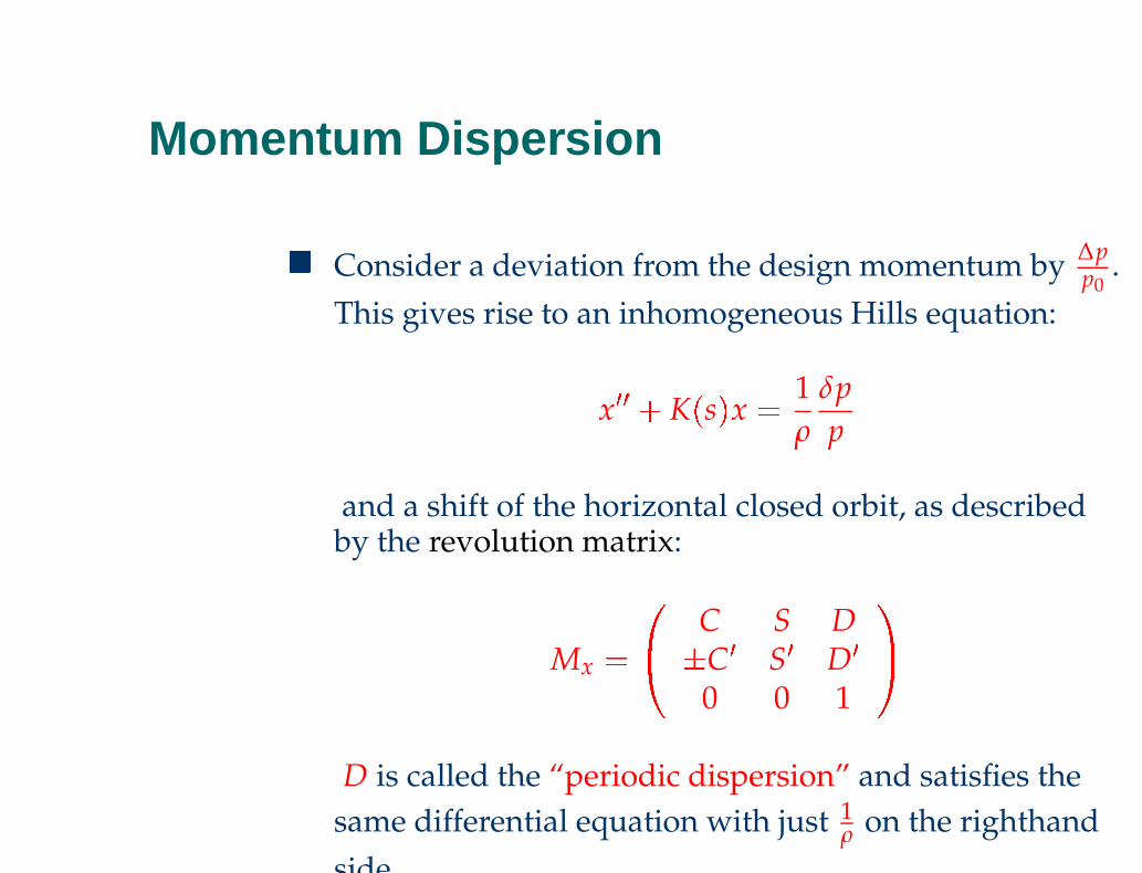
Consider a deviation from the design momentum by ∆pp0

.This gives rise to an inhomogeneous Hills equation:

x

� � � K�

s�

x � 1ρ

δpp

and a shift of the horizontal closed orbit, as describedby the revolution matrix:

Mx

�

C S D

�

C

�

S

�

D

�

0 0 1

D is called the “periodic dispersion” and satisfies thesame differential equation with just 1

ρ on the righthandside.

Dispersion function

�

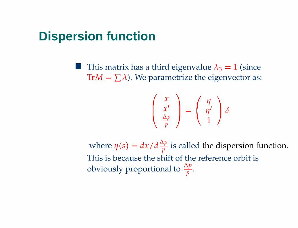
This matrix has a third eigenvalue λ3� 1 (since

TrM �

∑ λ). We parametrize the eigenvector as:

�

xx

�

∆pp

� �ηη

�

1δ

where η

�

s

�

� dx/d ∆pp is called the dispersion function.

This is because the shift of the reference orbit isobviously proportional to ∆p

p .

Dispersion function

�

Solving the eigenvector equation, we get

η �

�

1 � S

� �

D � SD�

2 � C � S�

��

1 � S

� �

D � SD

�

2

�

1 � 12 TrM

�

�

�

1 � S

� �

D � SD

�

2

�

1 � cos 2πQ

� ��

1 � S

� �

D � SD

�

4 sin2 πQ

�

Again we see the necessity to avoid integer Q. In fact,any “simple” rational number for either QH or QV isbad and may lead to resonances where the beam blowsup, because an off-momentum particle gets the samekick in the same phase at every few turns.

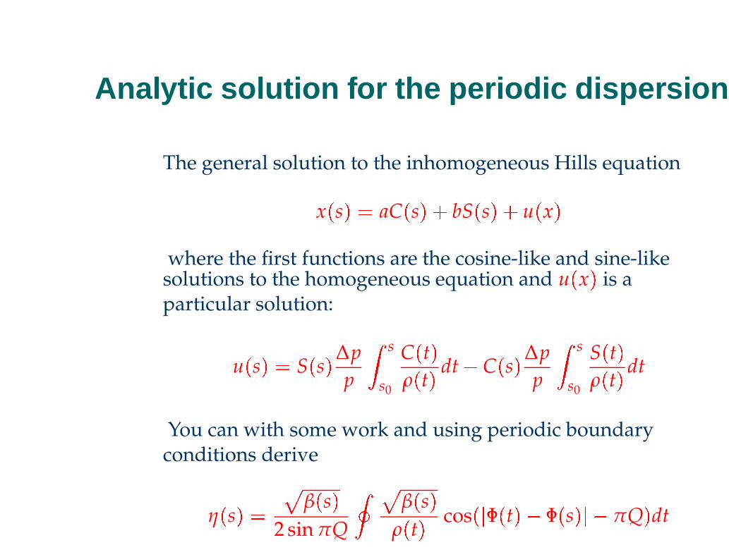
Analytic solution for the periodic dispersion

The general solution to the inhomogeneous Hills equation

x

�

s

�

� aC

�

s

� � bS�

s� � u�

x

�

where the first functions are the cosine-like and sine-likesolutions to the homogeneous equation and u

�

x

�

is aparticular solution:

u

�

s

�

� S

�

s� ∆p

p

s

s0

C

�

t

�

ρ

�

t

� dt � C

�

s

� ∆pp

s

s0

S

�

t

�

ρ

�

t

� dt

You can with some work and using periodic boundaryconditions derive

η�

s

�

�

β

�

s

�

2 sin πQβ

�

s

�

ρ

�

t

� cos

��

Φ

�

t

�

� Φ

�

s

� �

� πQ

�

dt

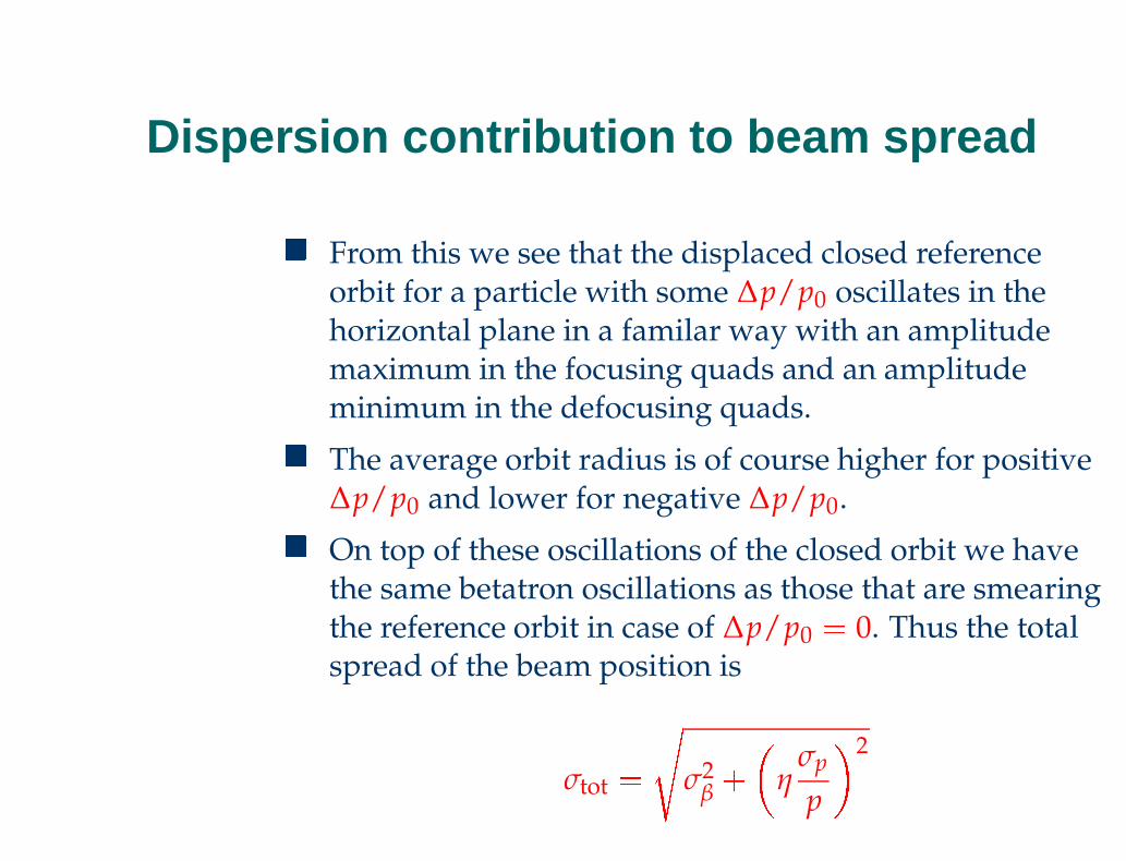
Dispersion contribution to beam spread

�

From this we see that the displaced closed referenceorbit for a particle with some ∆p/p0 oscillates in thehorizontal plane in a familar way with an amplitudemaximum in the focusing quads and an amplitudeminimum in the defocusing quads.

�

The average orbit radius is of course higher for positive∆p/p0 and lower for negative ∆p/p0.

�

On top of these oscillations of the closed orbit we havethe same betatron oscillations as those that are smearingthe reference orbit in case of ∆p/p0

� 0. Thus the totalspread of the beam position is

σtot

� σ2β

�

ησp

p

2

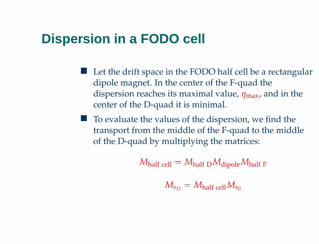
Dispersion in a FODO cell

�

Let the drift space in the FODO half cell be a rectangulardipole magnet. In the center of the F-quad thedispersion reaches its maximal value, ηmax, and in thecenter of the D-quad it is minimal.

�

To evaluate the values of the dispersion, we find thetransport from the middle of the F-quad to the middleof the D-quad by multiplying the matrices:

Mhalf cell

� Mhalf DMdipoleMhalf F

MsD

� Mhalf cell Ms0

Dispersion in a FODO cell

�

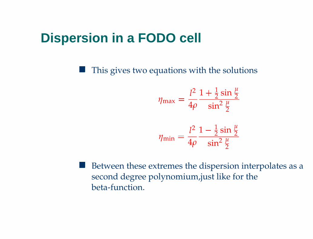
This gives two equations with the solutions

ηmax

� l2

4ρ

1 � 12 sin µ

2sin2 µ

2

ηmin

� l2

4ρ

1 � 12 sin µ

2sin2 µ

2

�

Between these extremes the dispersion interpolates as asecond degree polynomium,just like for thebeta-function.

Momentum compaction factor

�

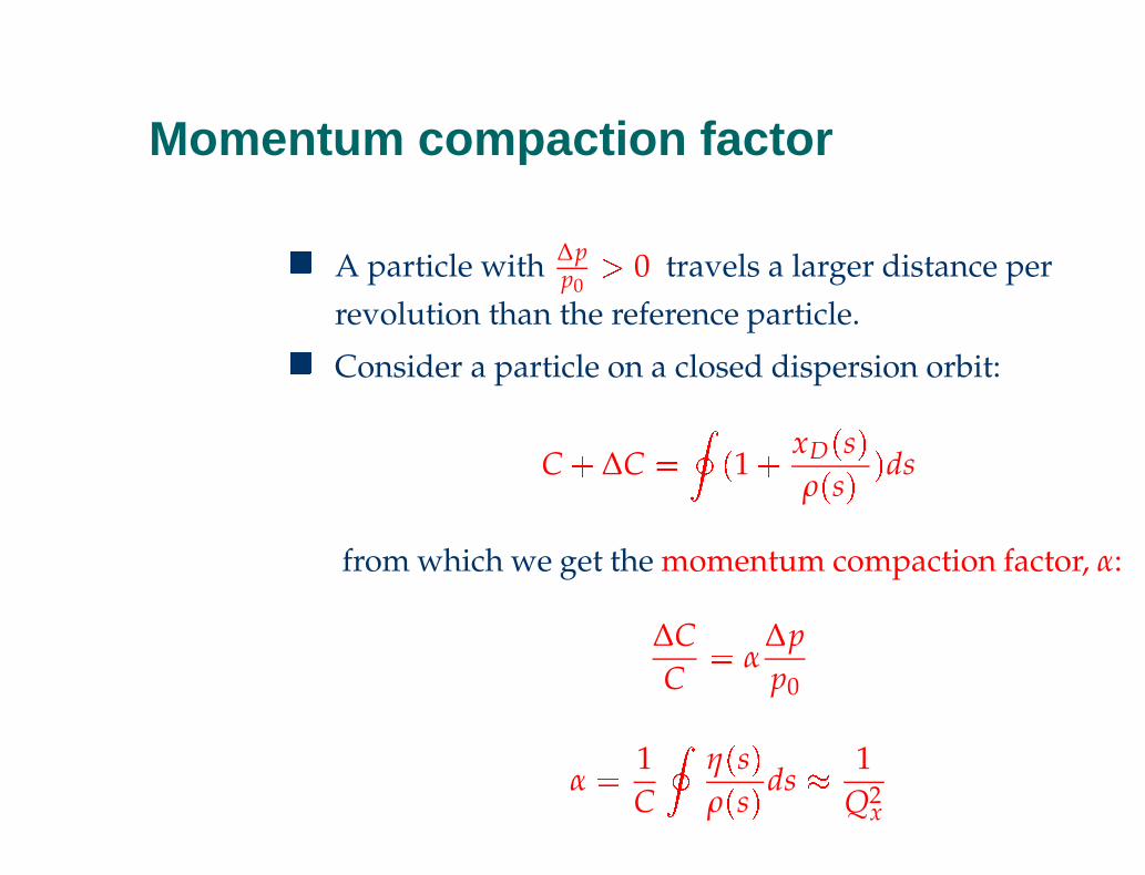
A particle with ∆pp0

� 0 travels a larger distance perrevolution than the reference particle.

�

Consider a particle on a closed dispersion orbit:

C �

∆C �

�

1 � xD

�

s

�

ρ

�

s

�

�

ds

from which we get the momentum compaction factor, α:

∆CC

� α∆pp0

α � 1C

η

�

s

�

ρ

�

s

� ds � 1Q2

x

Momentum compaction factor

�

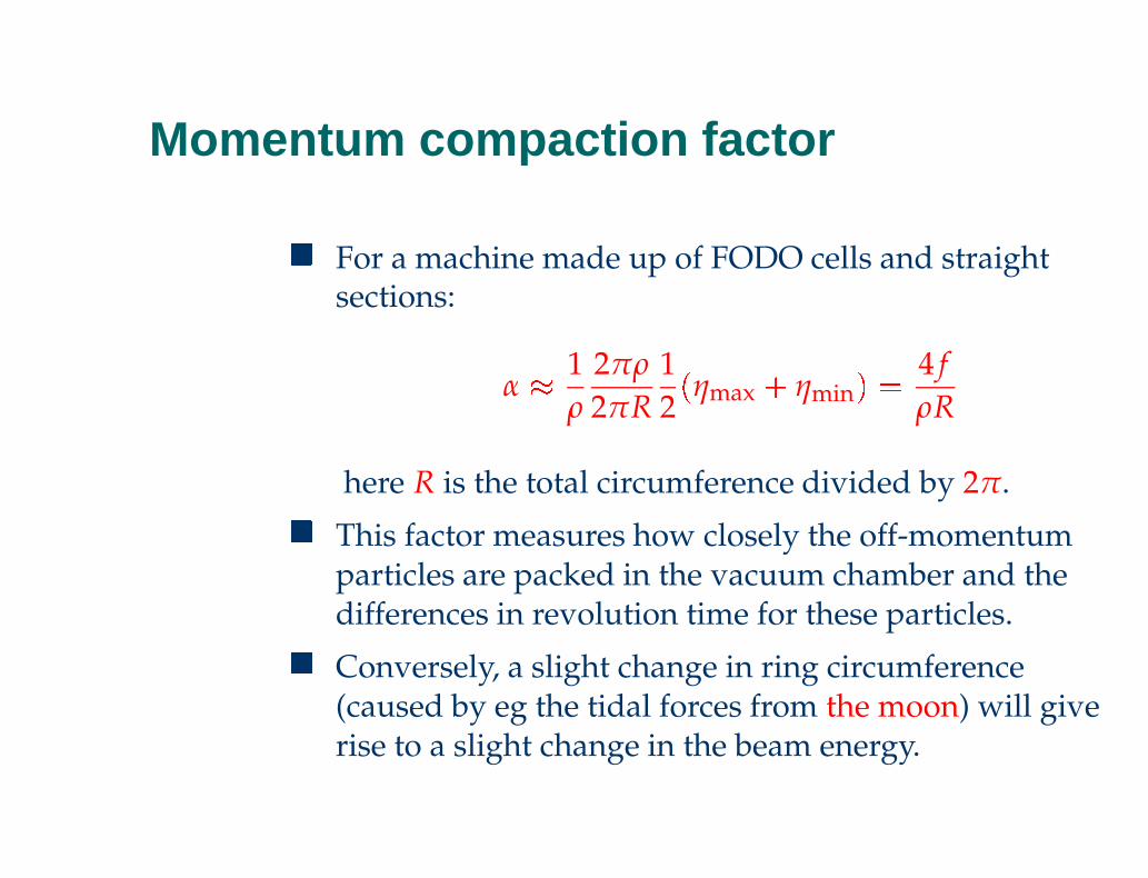
For a machine made up of FODO cells and straightsections:

α � 1ρ

2πρ

2πR12

�

ηmax�

ηmin

�

� 4 fρR

here R is the total circumference divided by 2π.

�

This factor measures how closely the off-momentumparticles are packed in the vacuum chamber and thedifferences in revolution time for these particles.

�

Conversely, a slight change in ring circumference(caused by eg the tidal forces from the moon) will giverise to a slight change in the beam energy.

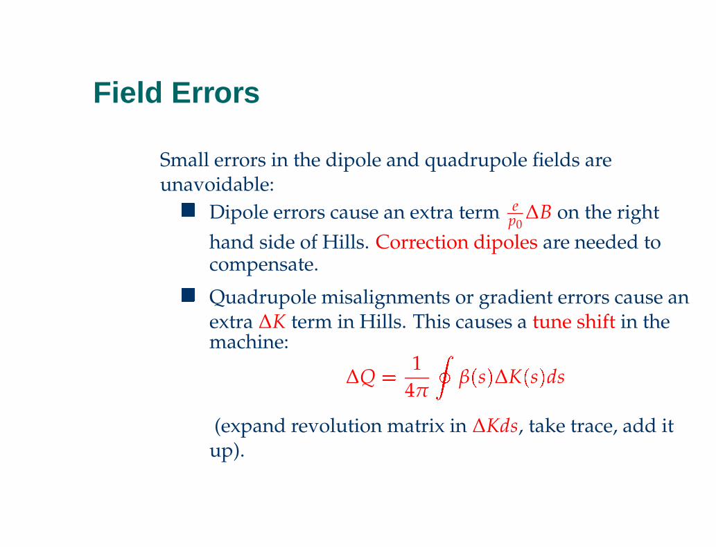
Field Errors

Small errors in the dipole and quadrupole fields areunavoidable:

�

Dipole errors cause an extra term ep0

∆B on the righthand side of Hills. Correction dipoles are needed tocompensate.

�

Quadrupole misalignments or gradient errors cause anextra ∆K term in Hills. This causes a tune shift in themachine:

∆Q � 14π

β

�

s

�

∆K

�

s

�

ds

(expand revolution matrix in ∆Kds, take trace, add itup).

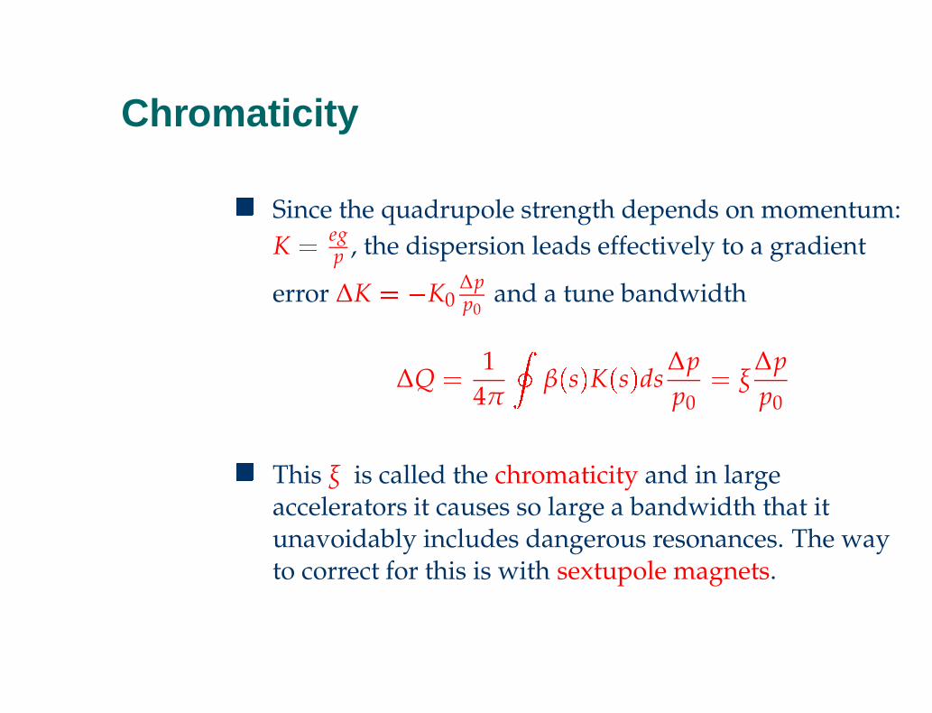
Chromaticity

�

Since the quadrupole strength depends on momentum:K � eg

p , the dispersion leads effectively to a gradient

error ∆K � � K0∆pp0

and a tune bandwidth

∆Q � 14π

β�

s�

K

�

s

�

ds∆pp0

� ξ∆pp0

�

This ξ is called the chromaticity and in largeaccelerators it causes so large a bandwidth that itunavoidably includes dangerous resonances. The wayto correct for this is with sextupole magnets.

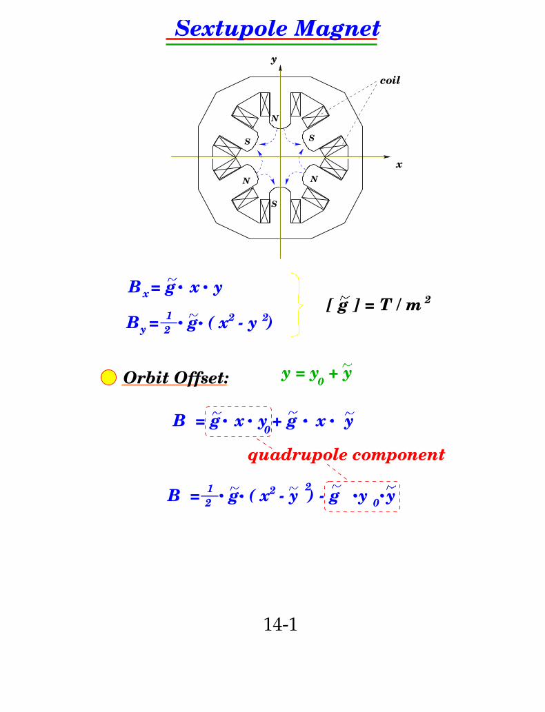
N

S

N

S

N

2

S

coil

x

y

Orbit Offset:

B = g x y + g x y0

y = y + y0

B = g x y

1

2B = g ( x - y )22

x

y

Sextupole Magnet

1

22 2

0B = g ( x - y ) - g y y

quadrupole component

[ g ] = T / m

14-1

p

p> 0

∆

0

p

p

∆

0

< 0

p

p

∆

0

p

p

∆

0

p

p

∆

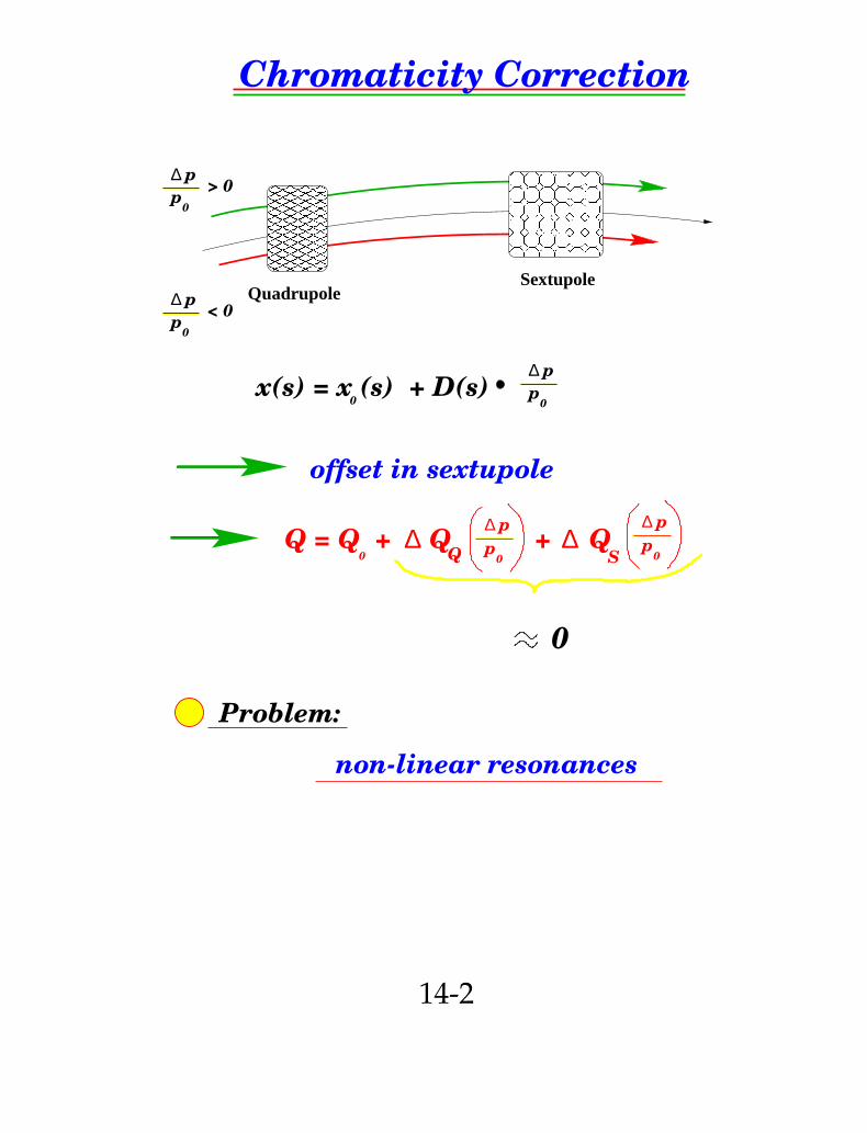
0Q = Q + Q + Q

0

non-linear resonances

∆ ∆Q S

������������������������������������������������������������������������������������������

������������������������������������������������������������������������������������������

������������������������������������������������������������������������������������������������������������

������������������������������������������������������������������������������������

Chromaticity Correction

SextupoleQuadrupole

offset in sextupole

x(s) = x (s) + D(s)0

0

Problem:

14-2

Exercise: Design an accelerator

�

When designing a new accelerator, you must firstconsider the physics that you want to do and then themoney needed to do it.

�

Let us here do it the other way around. Imagine wehave 200Mkr and therefore propose a modestaccelerator providing 1 GeV protons or electrons. Alinear accelerator will inject 200 MeV particles into a

� 35m circumference ring. Here the particles are storedand accelerated them to 1 GeV. Two 3m long straightsections are reserved, one for injection and accelerationand one for extraction to anybody with a good idea forusing the beam. .

Bending fields and gradients

�

Consider a FODO lattice with dipoles put in the driftspaces. Looking at the available money you give upsuperconducting technology and settle on conventionaldipole magnets with B � 1 Tesla (the maximum you candream of in this technology is 2 Tesla).

�

For the quadrupoles we choose a field gradient of10T/m (maximum is 20 T/m) and we hope that thesecan be made to a length of only 30cm. That will result ina focusing strength of k � eg

p

� 3m � 2, and a focal length

of f � 1kl

� 1.1m.

�

The beam pipe should be smaller than 10cm in order notto need too bulky magnets.

The phase advance and beta function

�

The length occupied by bending magnets must fulfilp � 0.3Bρ

� Cdipole

� 21m. With ten cells we get aFODO cell of length L � 2.1m � 0.6m � 2.7m and a totallength of C � 33m.

�

From sin µ2

� L4 f

� 0.6136 we get the phase advance percell µ � 76

�

(actually the optimal value) and the tuneQ � 2.1.

�

Now we can find the maximum of the beta-function (inthe F quad):

βmax

� L1 � sin µ

2sin µ

� 4.5m

wheras the average beta is approximately�

β

� � RQ

� 2.4m.

Emittance and beam-pipe

�

Let us aim at a beam emittance of 10π mm mrad. Wethen get the maximal beam size just from betatronoscillations:

xmax

�

�

ε βmax

� 1.2cm

�

This is good, but remember that we inject at 200 MeVwhere the beam emittance is five times higher. Thus ourbeampipe must be at least 12cm in diameter.

�

For the momentum compaction factor, we get α � 0.11.With a circumference of 33m, including straightsections, and a 1 percent momentum spread this leads toa variation of 5mm in radius on top of the 1.2cm above.

Chromaticity

�

For the chromaticity we get

ξ � �

14π

N1f

�

βmax � βmin

�

� � 3

with ∆pp0

� 10 � 2, this leads to a tune shift ∆Q � � 0.03unless correction sextupoles are introduced. This willmove the tune rather dangerously near the integer valueof 2.

�

Since the beam-pipe is on the large side, it would payoff to go through another iteration with slightly more(eg 12) cells and therefore a smaller length per cell andsmaller beta. The tune would also be a little larger.