Introduction: The first location problem? P1 P2 = (a2...

1

Introduction: The first location problem?

Early in the 17th century, Fermat (1601 - 1665) posed the following problem at the end of an

essay on maxima and minima (Kuhn, 1967):

"Let he who does not approve of my method attempt the solution of the following problem:

Given three points in the plane, find a fourth point such that the sum of its distances to the

three given points is a minimum."

Donote the three given points by P1 = (a1, b1), P2 = (a2, b2), and P3 = (a3, b3), and let X

= (x, y) be the fourth point to be found. The sum of the distances from X to the three given

points is given by the function:

f(X) = d(X,P1) + d(X,P2) + d(X,P3),

where d(X,Pi) = (x – ai)2 + (y – bi)2 is the Euclidean distance for i = 1, 2, 3.

The problem is to minimize f(X). (Figure 1)

P1

P2

P3X

Figure 1

2

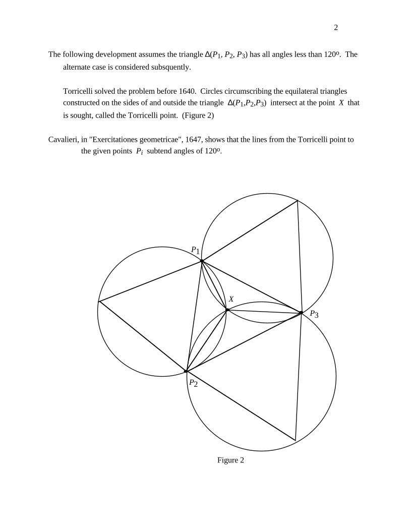
The following development assumes the triangle ∆(P1, P2, P3) has all angles less than 120o. The

alternate case is considered subsquently.

Torricelli solved the problem before 1640. Circles circumscribing the equilateral triangles

constructed on the sides of and outside the triangle ∆(P1,P2,P3) intersect at the point X that

is sought, called the Torricelli point. (Figure 2)

Cavalieri, in "Exercitationes geometricae", 1647, shows that the lines from the Torricelli point to

the given points Pi subtend angles of 120o.

P1

P2

P3

X

Figure 2

3

Simpson, in "Doctrine and Application of Fluxions", 1750, proved that the three lines joining the

outside vertices of the equilateral triangles defined above to the opposite vertices of the given

triangle intersect at the Torricelli point. The three lines are called Simpson lines. (Figure 3)

P1

P2

P3

X

Sim

pson

line

Simpson line

Simpson line

Figure 3

Heinen, in 1834 proved that the lengths of the three Simpson lines are equal and equal to the

minimum sum of distances.

Observe that if one of the angles of ∆(P1, P2, P3) is greater than 120o, then the three Simpson

lines intersect outside ∆(P1, P2, P3), indeed outside any equilateral triangle circumscribing

∆(P1, P2, P3). The case of having one angle greater than 120o is dealt with using properties

of mathematical programming.

Heinen also proved that for a triangle in which one angle is greater than or equal to 120o, the

vertex of this angle is the minimizing point.(Figure 4)

4

P1

P2

P3

X =

Figure 4

Fasbender, in 1846 proved that the perpendiculars to the Simpson lines through the three

given points are the sides of the largest equilateral triangle circumscribing these points, and

that the altitude of this triangle equals the minimum sum of distances. (Figure 5)

P1

P2

P3

XSimpson line

Sim

pson

line

Simpson line

Figure 5

5

Fasbender's results leads to a dual problem: Find the largest equilateral triangle circumscribing the

given triangle ∆(P1,P2,P3).

Restrict consideration to the case where the solution lies inside the triangle ∆(P1,P2,P3).

Lemma 1-1 : Let Z be any point interior to an equilateral triangle ∆(Z1,Z2,Z3) with altitude h.

Let hi be the length of the perpendicular from Z to the side opposite Zi. Then h = h1 + h2 +

h3.

Z

Z1

Z2

Z3

h

h1

h2

h3

Figure 6

Proof : In Figure 6, the area of ∆(Z1, Z2, Z3) = area of ∆(Z, Z2, Z3) + area of ∆(Z1, Z, Z3) +

area of ∆(Z1, Z2, Z). Thus h2

3 =

h

3 (h1 + h2 + h3) and the lemma is proved.

6

Lemma 1-2 : (Weak duality) Given three points P1, P2, P3 in the plane and any equilateral

triangle with altitude h circumscribing ∆(P1, P2, P3), for any point X interior to the

equilateral triangle,

h ≤ d(X,P1) + d(X,P2) + d(X,P3).

Proof: For each i, construct a perpendicular from X to the side of the equilateral triangle

passing through Pi, and let hi be the length of the perpendicular. (Figure 7) Then hi ≤d(X,Pi) since the leg of a right triangle is no longer than the hypotenuse. Apply Lemma 1.

P1

P2

P3

X

2h

3h1h

d(X,P )1

d(X,P )3

d(X,P )2

Figure 7

7

Lemma 2 shows that the altitude of any circumscribing equilateral triangle is less than or equal the

sum of distances from the Pi to any point interior to ∆(P1, P2, P3).

In the proof of Lemma 2, observe that hi = d(X,Pi) iff the line segments X,Pi are

perpendicular to the sides of the equilateral triangle. This occurs when the line segments

X,Pi subtend angles of 120o at X.

Theorem 1-1: The three Simpson lines intersect at the point X. The angles formed at X are all

equal to 60o. (Figure 5)

Theorem 1 may be proved by elementary geometry.

The geometrical approach presented above is limited to 3 given points. For n > 3, and more

general functions of distance, mathematical programming techniques are used.

Exercise: Use straight edge and compass to construct the Torricelli point for the following three

points.

P12

P

3P

Exercise: Attempt to construct the Torricelli point when the triangle ∆(P1, P2, P3) has one angle

greater than 120o.

8

The generalized Fermat problem, or Steiner - Weber problem

Extend the Fermat problem by allowing more than three points, by allowing positive weights

associated with each point, and by allowing the points to be placed anywhere in the plane.

Given distinct points Pi = (ai, bi) in the plane, and positive weights wi, for i = 1, . . . n. The

problem is to find a point X = (x, y) that minimizes the weighted sum of Euclidean distances

from X to the given points. Let f(X) = ∑i=1

nwid(X,Pi) . The generalized Fermat problem is

to minimize f(X).

This problem is also called the "Weber" problem because the economists Alfred Weber considered

it in Uber den Standort der Industrien in 1909. In their book What is Mathematics (1941),

Courant and Robins call this the "Steiner" problem because of the contributions made by

Steiner. It is also called the "minisum" problem in the location literature.

Observe that since the distance function d(X,Pi) is a convex function of X, and the weighted sum

of convex functions is convex, then f(X) is a convex function of X.

If the n distinct points Pi are not collinear, f(X) is a strictly convex function of X.

If the n distinct points Pi are not collinear, f(X) has a unique minimum point.

If the n distinct points Pi are collinear, then f(X) is a piece-wise linear, convex function of

X on the line through the points Pi, and is strictly convex elsewhere. This case is handled

subsequently. The points are assumed to be non collinear for the remainder of this

development.

Necessary and sufficient conditions for a point X to be an optimal location are developed next.

These conditions lead to several properties of the optimal solution, and to an algorithm for

iterating to the optimal solution.

9

Consider the mechanical analog of the generalized Fermat problem. Holes are drilled through a

table top at positions corresponding to the given points Pi. For each i, a string is placed

through the hole corresponding to Pi, and a weight wi is attached to the string. The strings

are tied in a common knot on top of the table. Assuming no friction, and negligible weight to

each string, the equilibrium position of the knot is the minimum location for X. (Figure 8)

This model is also called Varignon's Frame, and was suggested by Georg Pick in his

Mathematical Appendix to Weber's book.

X1P

3P

2P

4P

5P

w1

w2

w3

w4

w5

Figure 8

Each string corresponds to a vector from X to Pi, given by (Pi – X). Normalizing the length

of each vector (Pi – X) and multiplying by the weight wi gives a vector wi (Pi – X)

d(X,Pi) of

magnitude of wi, which corresponds to the force generated by the weight wi acting along

each string from X to Pi.

10

The resultant of all the forces along the strings at a point X is given as follows.

If X ≠ Pi the resultant force R(X) at X is given by:

R(X) = ∑i=1

n

w i (P i – X )d(X,Pi)

provided X ≠ Pi for all i.

If X = Pj for some j = 1, . . . n, define Rj as the vector sum of all forces from Pj to Pi

for i ≠ j, but disregarding the force wj at Pj :

Rj = ∑i=1 i≠j

n

w i (Pi – Pj)d(Pj,Pi)

.

Define the resultant force R(Pj) at Pj to incorporate the force wj as follows:

R(Pj) = max( |Rj| – wj, 0 )Rj|Rj|

.

Thus, if wj ≥ |Rj| , then R(Pj) = 0, else, there is a resultant vector in the direction of Rj

with magnitude |Rj| – wj.

Theorem 1-2 : The point X minimizes f(X) iff R(X) = 0.

Proof : If X is not a vertex, then the convexity and differentiability of f imply that the first order

condition ∇ f(X) = R(X) = 0 is necessary and sufficient for X to be a minimum.

If X = Pj for some j, consider the change in f along the direction Z from Pj to Pj + tZ

where |Z| = 1 and t ≥ 0.

Direct calculation shows that ddt f(Pj + tZ) = wj – RjZ for t = 0.

Hence the direction of greatest decrease is Z = Rj|Rj|

. Thus Pj is a local minimum iff

wj – RjRj|Rj|

≥ 0, i.e., if the directional derivative is nonnegative in the direction of greatest

decrease, then the directional derivative is nonnegative in all directions. However, wj – RjRj|Rj|

= wj – RjRj|Rj|

= wj – |Rj| ≥ 0 implies R(Pj) = 0.

11

Example: Suppose n = 3, all wi = 1, and the triangle ∆(P1, P2, P3) has no angle greater than

120o. A zero resultant force R(X) at a point X ≠ Pi implies that the normalized vectors(P i – X )d(X,Pi)

subtend angles of 120o.

P12P

3P

X

If the triangle ∆(P1, P2, P3) has one angle greater than 120o, say at P1, the resultant vector

R1 = (P2 – P1)d(P2,P1) +

(P3 – P1)d(P3,P1) has magnitude < 1 = w1, and P1 is optimal.

P1

2P3P R1

12

Example: Suppose n = 4, all wi are equal, and all four points Pi are extreme points to the

convex hull of the Pi, i.e., none of the given points Pj is interior to the triangle formed by the

remaining three points. Then the lines connecting "opposite" points, see Figure 9, intersect at

a point X interior to the convex hull of the four points.

The conditions of optimality state that X is the optimal solution since R(X) = 0, i.e., the

normalized resultant forces from X to each Pi "cancel out" and the resultant force is zero.

X1

P

3P

2P

4P

If one of the given four points, say Pj, is interior to the triangle formed by the remaining three

points, then X = Pj is the optimal solution, since |Rj| < 1 = wj.

1P

3P

2P

4P

R1

13

Corollary 1-1 : (Majority Property) If wj ≥ ∑i=1 i≠j

nwi for some j, then Pj is the optimal location.

Proof : Observe that |Rj| = | ∑i=1 i≠j

n

w i P i – P jd(Pj,Pi)

| ≤ ∑i=1 i≠j

n

w i |Pi – Pj|d(Pj,Pi)

= ∑i=1 i≠j

nw i .

If wj ≥ ∑i=1 i≠j

nwi ≥ |Rj| , then R(Pj) = 0, and Pj is the optimal solution.

The following stronger result is proven in Kuhn and Kuenne (1962) and Hamacher (1995).

Theorem 1-3 : Pj is the optimal location if and only if

wj2 ≥ ( ∑i=1 i≠j

n

w i ai – ajd(Pj,Pi)

)2 + ( ∑i=1 i≠j

n

w i b i – bjd(Pj,Pi)

)2 .

Theorem 1-4 : If the point X minimizes f(X), then X is in the convex hull of the points Pi.

Proof : If the point X is a vertex Pi, then it is trivially in the convex hull. Otherwise, the

condition R(X) = 0 yields

∑i=1

n

wiPi

d(X,Pi) = ∑

i=1

n

wiX

d(X,Pi)

or X = ∑i=1

n

wiPi

d(X,Pi) / ∑

i=1

n

wi

d(X,Pi) (*)

Define λi = wi

d(X,Pi) / ∑

i=1

n

wi

d(X,Pi) so that X = ∑

i=1

n

λiPi , and ∑i=1

n

λi = 1, which is a

convex combination of the points Pi.

Corollary 1-2 : If the point X minimizes f(X) and is not a vertex, then X is not on the

boundary of the convex hull.

Proof : This follows because the λi > 0 for each i.

14

Iterative solution methods for the weighted Euclidean distance minisum problem

An iterative method is suggested by expression (*). This method attempts to find an X that

satisfies the conditions of optimality.

Xk+1 = ∑i=1

n

wiPi

d(Xk,Pi) / ∑

i=1

n

wi

d(Xk,Pi) .

A suitable starting point is given by X0 = ∑i=1

n

wiPi / ∑i=1

nwi which is the center of gravity of

the Pi.

This iterative scheme is equivalent to the gradient method with specified step length (Kuhn,

1967). Note that –R(X) is the gradient of f(X) when it exists. This method was first

suggested by E. Weiszfeld (1937). Convergence is proved by Kuhn (1973).

Another approach taken by Love and Morris (1975) approximates the nondifferentiable Euclidean

distance function by a differentiable function called the hyperbolic approximation:

dε(X, Pi) = [(x – ai)2 + (y – bi)2 + ε ]1/2 for ε a small positive real number.

The generalized Fermat problem is given by

min fε(X) = ∑i=1

nwidε(X,Pi) .

Love and Morris show give convergence results and computational experience that show

fε(X) → f(X) as ε → 0.

15

Generalized Fashbender duality

A dual to the generalized Fermat problem is developed that generalizes the geometric dual

developed for the case with n = 3 and all weights equal to 1.

Given distinct points Pi = (ai, bi) in the plane, and positive weights wi, for i = 1, . . . n.

Let Ui = (ui, vi) denote n two-dimensional vectors. The dual to the generalized Fermat

problem asks for the vectors Ui which maximize

g(U1, U2, . . . , Un) = ∑i=1

n

Ui.Pi

s.t. ∑i=1

n Ui = 0 (4)

|Ui| ≤ wi for i = 1, . . . , n. (5)

Theorem 1-5 : (weak duality) For any X and any set of Ui, satisfying (4) and (5),

g(U1, U2, . . . , Un) ≤ f(X).

Proof : g(U1, U2, . . . , Un) = ∑i=1

n

Ui.Pi = ∑i=1

n

Ui.Pi – ∑i=1

n Ui X = ∑

i=1

n U i(P i – X ) .

≤ ∑i=1

n |Ui| |Pi – X| (by the Schwartz inequality, Ui(Pi – X) ≤ |Ui| |Pi–X| )

≤ ∑i=1

nwid(X,Pi) = f(X).

16

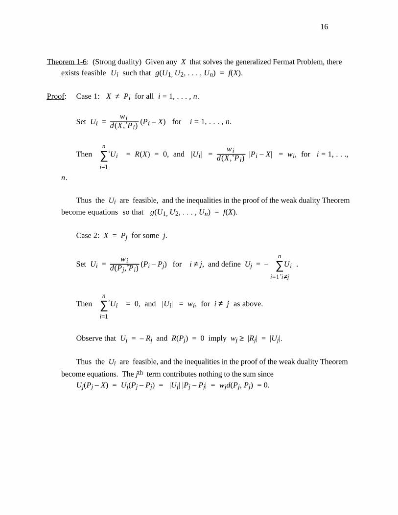
Theorem 1-6 : (Strong duality) Given any X that solves the generalized Fermat Problem, there

exists feasible Ui such that g(U1, U2, . . . , Un) = f(X).

Proof : Case 1: X ≠ Pi for all i = 1, . . . , n.

Set Ui = wi

d(X , Pi) (Pi – X) for i = 1, . . . , n.

Then ∑i=1

n Ui = R(X) = 0, and |Ui| =

wid(X , Pi)

|Pi – X| = wi, for i = 1, . . .,

n.

Thus the Ui are feasible, and the inequalities in the proof of the weak duality Theorem

become equations so that g(U1, U2, . . . , Un) = f(X).

Case 2: X = Pj for some j.

Set Ui = wi

d(Pj, Pi) (Pi – Pj) for i ≠ j, and define Uj = – ∑

i=1 i≠j

nUi .

Then ∑i=1

n Ui = 0, and |Ui| = wi, for i ≠ j as above.

Observe that Uj = – Rj and R(Pj) = 0 imply wj ≥ |Rj| = |Uj|.

Thus the Ui are feasible, and the inequalities in the proof of the weak duality Theorem

become equations. The jth term contributes nothing to the sum since

Uj(Pj – X) = Uj(Pj – Pj) = |Uj| |Pj – Pj| = wjd(Pj, Pj) = 0.

17

Theorem 1-7 : Given any feasible Ui which solve the dual program, there exists an X such that

g(U1, U2, . . . , Un) = f(X).

The proof may be found in Kuhn (1967), and is an application of the Kuhn-Tucker

conditions. The proof shows that any solution to the dual program provides a solution to the

generalized Fermat problem in the following manner. If all |Ui| = wi, then the lines through

Pi with directions Ui all go through X. To find X, two lines will suffice. Otherwise, at

most one Ui can satisfy |Ui| < wi, say for i = j. Then X = Pj.

How does the generalized dual relate to the geometric dual for the Fermat problem with n = 3 and

wi = 1?

Refer to Figure 7. Let Ui be a unit vector from X and perpendicular to the side of the

equilateral triangle circumscribing ∆(P1, P2, P3) which contains Pi for i = 1, 2, 3. Then

|Ui| = 1 and U1 + U2 + U3 = 0, so the Ui are feasible to the dual of the generalized

Fermat problem.

Observe that hi = Ui.(Pi – X) for i = 1, 2, 3, so that

h = ∑i

hi = ∑i

Ui.(Pi – X) = ∑i

Ui.Pi – X∑i

Ui = ∑i

Ui.Pi since ∑i

Ui = 0.

Thus the length of the altitude of the circumscribing equilateral triangle equals the value of the

objective function associated with the Ui.

Conversely, any feasible Ui determine a circumscribing equilateral triangle, with the same

equality holding.

Thus Fasbender's dual problem is a special case of the generalized dual problem.

19

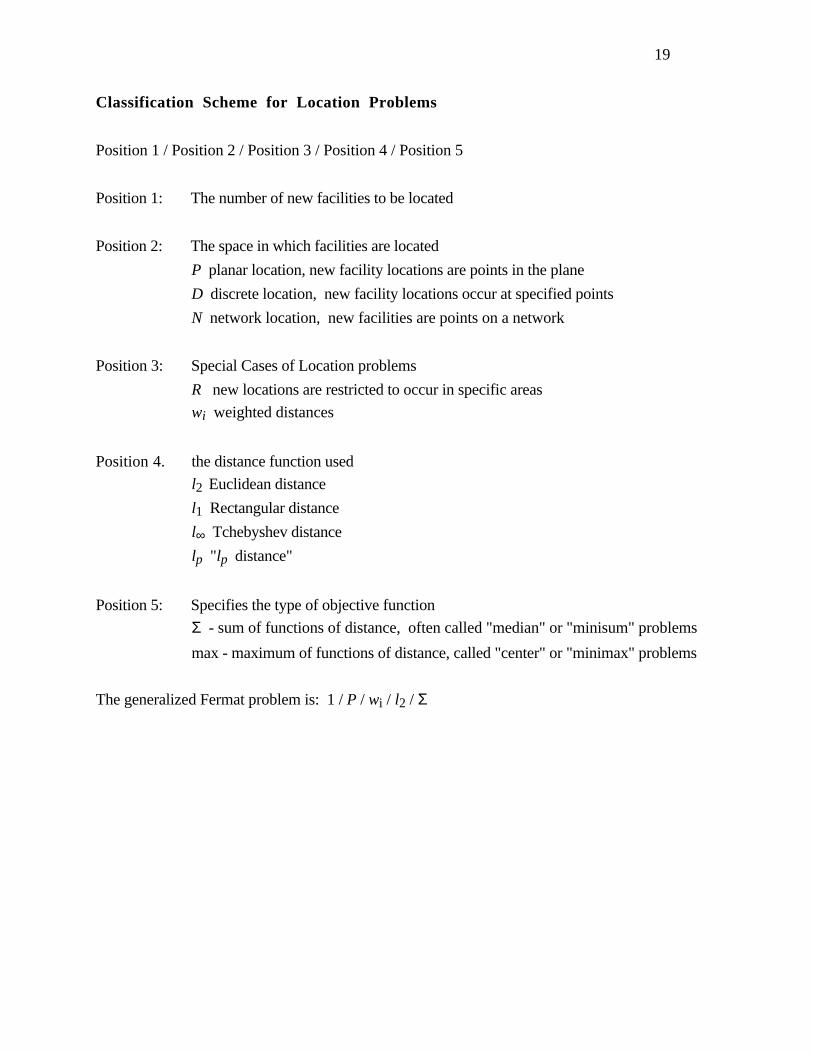
Classification Scheme for Location Problems

Position 1 / Position 2 / Position 3 / Position 4 / Position 5

Position 1: The number of new facilities to be located

Position 2: The space in which facilities are located

P planar location, new facility locations are points in the plane

D discrete location, new facility locations occur at specified points

N network location, new facilities are points on a network

Position 3: Special Cases of Location problems

R new locations are restricted to occur in specific areas

wi weighted distances

Position 4. the distance function used

l2 Euclidean distance

l1 Rectangular distance

l∞ Tchebyshev distance

lp "lp distance"

Position 5: Specifies the type of objective function

Σ - sum of functions of distance, often called "median" or "minisum" problems

max - maximum of functions of distance, called "center" or "minimax" problems

The generalized Fermat problem is: 1 / P / wi / l2 / Σ

20

The weighted, squared Euclidean distance minisum problem: 1 / P / w i / l22 / Σ


The problem is to find a point X = (x, y) that minimizes the weighted sum of the squared

Euclidean distances from X to the given points.

Define the function f(X) by f(X) = ∑i=1

nwi[d(X,Pi) ]2

where [d(X,P1)] = (x – a1)2 + (y – b1)2.

The problem is to minimize f(X).

This problem has a closed form solution that is obtained from the the first order conditions for

optimality.

∂f

∂x = 2 ∑

i=1

nwi(x – ai) = 0 and

∂f

∂y = 2 ∑

i=1

nwi(y – bi) = 0.

Solving for x and y yield:

which yield x =

∑i=1

nwiai

∑i=1

nwi

and y =

∑i=1

nwibi

∑i=1

nwi

.

21

The weighted rectangular distance minisum problem: 1 / P / w i / l1 / Σ


The problem is to find a point X = (x, y) that minimizes the weighted sum of the rectangular

distances from X to the given points.


nwil1(X,Pi)

where l1(X,Pi) = |x – ai| + |y – bi| is the rectangular distance from X to Pi.


Observe that

f(X) = ∑i=1

nwi(|x – ai| + |y – bi|) = ∑

i=1

nwi|x – ai| + ∑

i=1

nwi|y – bi| .

Define f1(x) = ∑i=1

nwi|x – ai| and f2(y) = ∑

i=1

nwi|y – bi| .

Then solutions X* to the problem min f(X) may be obtained by solving the independent

problems:

min f1(x) for x* and min f2(y) for y* and taking X* = (x*, y*).

Consider the problem min f1(x) = ∑i=1

nwi|x – ai| .

Suppose the set {ai, i = 1,. . ,n} of existing facility first coordinates contains k ≤ n distinct

values. Rename the k distinct values as a'j and order them so that a'1 < a'2 < . . < a'k.

Define s(j) = { i : ai = a'j } and define w'j = ∑i∈ s(j)

wi .

22

Then f1(x) = ∑i=1

nwi|x – ai| = ∑

j=1

kw'j|x – a'j| .

Observe that for any x* ∈ [a'1, a'k], and any x ∉ [a'1, a'k], f1(x) > f1(x*) so that all optimal

solutions lie in the interval [a'1, a'k].

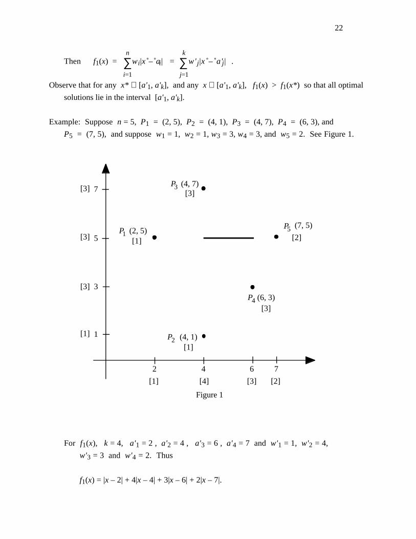
Example: Suppose n = 5, P1 = (2, 5), P2 = (4, 1), P3 = (4, 7), P4 = (6, 3), and

P5 = (7, 5), and suppose w1 = 1, w2 = 1, w3 = 3, w4 = 3, and w5 = 2. See Figure 1.

(2, 5)

(4, 1)

(6, 3)

(4, 7)

2 4 6 7

[1]

[1]

[3]

[3]

[2]

[1] [4] [3] [2]

[1]

[3]

[3]

[3] 7

5

3

1

P1

P2

P3

P4

(7, 5)P5

Figure 1

For f1(x), k = 4, a'1 = 2 , a'2 = 4 , a'3 = 6 , a'4 = 7 and w'1 = 1, w'2 = 4,

w'3 = 3 and w'4 = 2. Thus

f1(x) = |x – 2| + 4|x – 4| + 3|x – 6| + 2|x – 7|.

23

The function f1(x) = |x – 2| + 4|x – 4| + 3|x – 6| + 2|x – 7| is shown in Figure 2.

2 4 6 7

[1] [4] [3] [2]

14

30

20

x

Figure 2

To find a minimum solution to f1(x), we apply standard minimization techniques. The critical

points of f1(x) are the points where the derivative of f1(x) is zero, and the points where f1(x)

has no derivative.

Observe that the function f1(x) is differentiable for all x ≠ a'j, j = 1, . . . , k.

Suppose a'p < x < a'p+1 for some p = 1, . . , k–1. Then f1(x) may be written as:

f1(x) = ∑j=1

pw'j (x – a'j) + ∑

j=p+1

kw'j (a'j – x) , which shows that f1(x) is piecewise

linear.

24

The derivative of f1(x) is given by f'1(x) = ∑j=1

pw'j – ∑

j=p+1

kw ' j .

Thus x is a critical point if a'p < x < ap+1 and f'1(x) = 0, i.e. ∑i=1

pwi = ∑

i=p+1

kw i .

Since f1(x) is convex, a point x such that f'1(x) = 0 is a global minimum.

Observe that f1(x) is not differentiable at the points a'j, j = 1, . . . , k. Thus the points a'j,

j = 1, . . . , k, are critical points.

The critical point a'p is a minimum point if f1(x) is nonincreasing, i.e., f'1(x) ≤ 0, for

x < a'p, and if f1(x) is nondecreasing, i.e., f'1(x) ≥ 0, for x > a'p.

That is, if f'1(x) = ∑j=1

p-1w'j –∑

j=p

kw'j ≤ 0 and f'1(x) = ∑

j=1

pw'j – ∑

j=p+1

kw'j ≥ 0.

Here we use the convention that ∑j=1

p-1w'j = 0 if p = 1, and ∑

j=p+1

kw'j = 0 if p = k.

In summary, if for some p = 1, . . . , k,

(1) ∑j=1

p-1w'j –∑

j=p

kw'j < 0 and ∑

j=1

pw'j – ∑

j=p+1

kw'j > 0, then a'p is a unique minimum point,

or (2) ∑j=1

pw'j – ∑

j=p+1

kw'j = 0, then all x such that a'p ≤ x ≤ ap+1 are minimum points.

For f1(x) in the expample, choose p = 2, and observe that ∑j=1

pw'j – ∑

j=p+1

kw'j = 5 – 5 =

0.

Thus all x such that 4 ≤ x ≤ 6 are optimal solutions.

25

The same approach is used for the subproblem min f2(y) = ∑i=1

nw i|y – bi| .

Suppose the set {bi, i = 1,. . ,n} of existing facility second coordinates contains l ≤ n distinct

values. Rename the l distinct values as b'j and order them so that b'1 < b'2 < . . < b'l.

Define s(j) = { i : bi = b'j } and define w"j = ∑i∈ s(j)

wi .

Then f2(x) = ∑i=1

nwi|x – bi| = ∑

j=1

lw"j|x – b'j| .

For f2(x), l = 4, b'1 = 1 , b'2 = 3 , b'3 = 5 , b'4 = 7 and w"1 = 1, w"2 = 3,

w"3 = 3 and w"4 = 3.

Thus f2(x) = |y – 1| + 3|y – 3| + 3|y – 5| + 3|y – 7|.

The function f2(x) = |y – 1| + 3|y – 3| + 3|y – 5| + 3|y – 7| is shown in Figure 3.

26

3 5 7

[1] [3] [3] [3]

16

36

20

x1

24

Figure 3

The optimality conditions are given as follows. For p = 1, . . . , l:

If ∑j=1

p-1w"j –∑

j=p

lw"j < 0 and ∑

j=1

pw"j – ∑

j=p+1

lw"j > 0, then b'p is a unique minimum point.

If ∑j=1

pw"j – ∑

j=p+1

lw"j = 0, then all y such that b'p ≤ y ≤ b'p+1 are minimum points.

For f2(x) in the example problem, choose p = 3, and observe that

∑j=1

p-1w"j –∑

j=p

lw"j = 4 – 6 < 0 and ∑

j=1

pw"j – ∑

j=p+1

lw"j = 7 – 3 > 0.

27

Thus y = b'3 = 5 is a unique optimal solution.

Thus the set of optimal solutions to min f(X) is { X = (x, y) : x ∈ [4, 6] and y = 5 }

and is shown by the bold line in Figure 1.

28

Linear Programming Approach to 1 / P / wi / l1 / Σ .

Consider the problem in the form min f(X) = min f1(x) + min f2(y), where

f1(x) = ∑j=1

kw'j|x – a'j| . and f2(x) = ∑

j=1

lw"j|x – b'j| .

Each subproblem may be represented as an equivalent linear program. Consider the problem

min ∑j=1

kw'j|x – a'j| and define variables pj and qj for j = 1, . . . , k. The linear program

may be written as:

min ∑j=1

kw ' j ( p j + q j )

s.t. x – a'j = pj – qj or x – pj + qj = a'j for j = 1, . . . , k

pj, qj ≥ 0 for j = 1, . . . , k.

The linear programming dual, with dual variables uj, j = 1, . . . , k may be written as:

max ∑j=1

k

a'juj

s.t. ∑j=1

k

uj = 0

uj ≤ w'j and – uj ≤ w'j or |uj| ≤ w'j for j = 1, . . . , k .

Observe that the dual problem has the same form as the dual of the generalized Fermat

problem. The properties of weak duality and strong duality hold for this primal - dual pair by

results of linear programming. The following result specifies strong duality to this particular

problem.

29

Suppose for some p = 1, . . . , k, that ∑j=1

p-1w'j < ∑

j=p

kw'j , and ∑

j=1

pw'j > ∑

j=p+1

kw ' j .

Thus a'p is a unique minimum solution. Define uj j = 1, . . . , k, as follows:

uj = – w'j for j = 1, . . . , p–1,

uj = w'j for j = p+1, . . . , k,

and up = ∑j=1

p-1w'j – ∑

j=p+1

kw ' j .

Theorem 1-8 : The point a'p minimizes f1(x) and the variables { u1, u2, . . . , uk } maximize

the dual, and their objective function values are equal.

Proof: ∑j=1

k

a'juj = ∑j=1

k

a'juj – a'p∑j=1

k

uj since ∑j=1

k

uj = 0

= ∑j=1

p-1uj(a'j – a'p) + ∑

j=p+1

kuj(a'j – a'p)

= ∑j=1

p-1w'j(a'p – a'j) + ∑

j=p+1

kw'j(a'j – a'p)

= f1(ap).

Observe that uj ≤ |w'j| for j ≠ p by definition. For up,

up = ∑j=1

p-1w'j – ∑

j=p+1

kw'j = ∑

j=1

p-1w'j – ∑

j=p

kw'j + w'p ≤ w'p

and up = ∑j=1

p-1w'j – ∑

j=p+1

kw'j = ∑

j=1

pw'j – ∑

j=p+1

kw'j – w'p ≥ w'p.

Thus up ≤ |w'p| and the set of uj defined above are dual feasible.

30

The one facility median problem with Tschebychev distance: 1 / P / w i / l∞ / Σ


The problem is to find a point X = (x, y) that minimizes the weighted sum of the

Tschebychev distances from X to the given points.


nwil∞(X,Pi)

where l∞(X,Pi) = max {|x – ai|, |y – bi|}


The approach to this problem is to transform the Tschebychev distance into the rectilinear

distance as prescribed by the following Lemma.

Consider a transformation T' that rotates the coordinate axes counter-clockwise through 45

degrees. The transformation T' is given by the nonsingular matrix T' = 12

1 –11 1 .

Property 1-1: l∞(X,Pi) = l1(T'(X),T'(Pi)).

Proof: l1(T(X),T(Pi)) = 12 | x – y – a + b | +

12 | x + y – a – b |

= 12 max { (x – y – a + b + x + y – a – b), ( x – y – a + b – x – y + a + b),

( – x + y + a – b + x + y – a – b), ( – x + y + a – b – x – y + a + b) }

= 12 max { 2(x – a), 2(–y + b), 2(y – b), 2(–x + a) }

= max { | x – a |, | y – b | } = l∞(X,Pi) .

Property 1-2: X is an optimal solution to min ∑i=1

nwi l∞(X,Pi) with objective function value z if

and only if T'(X) is an optimal solution to min ∑i=1

n

wi l1(T'(X),T'(Pi)) with objective

function value 2z.

The problem is transformed by T' into a problem with l1 distances and solved as above.

31

The one facility minisum problem with lp distance: 1 / P / w i / lp / Σ


The problem is to find a point X = (x, y) that minimizes the weighted sum of the lp

distances from X to the given points.


nwilp(X,Pi)

where lp(X,Pi) = [ |x – ai|p + |y – bi|p ]1/p


Observe that for p = 2, lp is the Euclidean distance, and for p = 1, l1 is the rectangular

distance. Also, limp→∞ lp = l∞ gives the Tschebychev distance.

Love and Morris (1972) show that US inter-city highway distances are closely predicted by

the function 1.15l1.78 .

It can be shown that the distance function lp(X,Pi) = [ |x – ai|p + |y – bi|p ]1/p is a convex

function in X.

Love and Morris (1975) define a hyperbolic approximation to lp that has continuous

derivatives everywhere: lpε(X,Pi) = [ |x – ai|p + |y – bi|p + ε ]1/p for ε > 0. They show

that lpε(X,Pi) is convex and that lpε(X,Pi) converges to lp(X,Pi) uniformly as ε → 0.

Then the ε – approximate one facility minsum objective function is given by:

fε(X) = ∑i=1

nwilpε(X,Pi) .

They used standard nonlinear techniques to minimize fε(X).

Morris and Verdini (1979) consider a different approximation that allows the development of

a Weiszfeld type algorithm. They define Lpε(X,Pi) = { [ |x – ai|2 + |y – bi|2 + ε ]p/2 }1/p

for ε > 0. Then Fε(X) = ∑i=1

nwiLpε(X,Pi) which is shown to be convex and have

continuous derivatives everywhere.

32

The gradients of Fε(X) yields

∂F

∂x = ∑

i=1

n

wi(x – ai)Lpε(X,Pi)1/p–1[(x – ai)2 + ε ]p/2–1

and∂F

∂y = ∑

i=1

n

wi(y – bi)Lpε(X,Pi)1/p–1[(y – bi)2 + ε ]p/2–1 .

The necessary conditions, ∂F

∂x = 0 and

∂F

∂y = 0, which are also sufficient since F is convex,

yield the following iterative expressions for x and y analogous to Weiszfeld.

xt+1 =

∑i=1

n

wiaiLpε(Xt,Pi)1/p–1[(xt – ai)2 + ε ]p/2–1

∑i=1

n

wiLpε(Xt,Pi)1/p–1[(xt – ai)2 + ε ]p/2–1

and yt+1 =

∑i=1

n

wibiLpε(Xt,Pi)1/p–1[(yt – bi)2 + ε ]p/2–1

∑i=1

n

wiLpε(Xt,Pi)1/p–1[(yt – bi)2 + ε ]p/2–1

.

Morris and Verdini show convergence properties and give computational results.

33

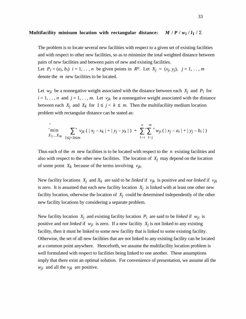
Multifacility minisum location with rectangular distance: M / P / w i / l1 / Σ

The problem is to locate several new facilities with respect to a given set of existing facilities

and with respect to other new facilities, so as to minimize the total weighted distance between

pairs of new facilities and between pairs of new and existing facilities.

Let Pi = (ai, bi) i = 1, . . , n be given points in Rn. Let Xj = (xj, yj), j = 1, . . , m

denote the m new facilities to be located.

Let wji be a nonnegative weight associated with the distance between each Xj and Pi for

i = 1, . . , n and j = 1, . . , m. Let vjk be a nonnegative weight associated with the distance

between each Xj and Xk for 1 ≤ j < k ≤ m. Then the multifaciliity medium location

problem with rectangular distance can be stated as:

minX1...Xm

∑1≤j<k≤m

vjk ( | xj – xk | + | yj – yk | ) + ∑1=i

n

∑1=j

m

wji ( | xj – ai | + | yj – bi | )

Thus each of the m new facilities is to be located with respect to the n existing facilities and

also with respect to the other new facilities. The location of Xj may depend on the location

of some point Xk because of the terms involving vjk.

New facility locations Xj and Xk are said to be linked if vjk is positive and not linked if vjk

is zero. It is assumed that each new facility location Xj is linked with at least one other new

facility location, otherwise the location of Xj could be determined independently of the other

new facility locations by considering a separate problem.

New facility location Xj and existing facility location Pi are said to be linked if wji is

positive and not linked if wji is zero. If a new facility Xj is not linked to any existing

facility, then it must be linked to some new facility that is linked to some existing facility.

Otherwise, the set of all new facilities that are not linked to any existing facility can be located

at a common point anywhere. Henceforth, we assume the multifacility location problem is

well formulated with respect to facilities being linked to one another. These assumptions

imply that there exist an optimal solution. For convenience of presentation, we assume all the

wji and all the vjk are positive.

34

The multifaciliity medium location problem with rectangular distance can separated into

independent subproblems in the variables xj and in the variables yj. These subproblems are:

SP(x) minX1...Xm

∑1≤j<k≤m

vjk | xj – xk | + ∑1=i

n

∑1=j

m

wji | xj – ai |

SP(y) minX1...Xm

∑1≤j<k≤m

vjk | yj – yk | + ∑1=i

n

∑1=j

m

wji | yj – bi |

Each subproblem can written as an equivalent linear programming problem. For the problem

SP(x), the linear program is obtained by introducing variables pjk, qjk, for 1 ≤ j < k ≤ m,

and rji, and sji for j = 1, . . ., n and i = 1, . . . , m.

min ∑1≤j<k≤n

vjk ( pjk + qjk ) + ∑1=i

n

∑1=j

m

wji ( rji + sji )

s.t. xj – rji + sji = aji i = 1, . . . , n, j = 1, . . . , m

xj – xk – pjk + qjk = 0 j = 1, . . . , m, k = j+ 1, . . . , m

pjk, qjk, rji, and sji ≥ 0.

Suppose the optimal solution is x*j j= 1, . . . , m with objective function value z(x*).

A similar linear program is obtained for the subproblem SP(y). Suppose the optimal solution

is y*j j= 1, . . . , m with objective function value z(y*). Then an optimal solution to the

original problem is given by X*j = (x*j, y*j) j= 1, . . . , m with z* = z(x*) + z(y*).

35

Multifacility minisum location with weighted Euclidean distance: M / P / w i / l1 /

Σ

The problem is to locate several new facilities with respect to a given set of existing facilities

and with respect to other new facilities, so as to minimize the total weighted distance between

pairs of new facilities and between pairs of new and existing facilities.

Let Pi = (ai, bi) i = 1, . . , n be given points in Rn. Let Xj = (xj, yj), j = 1, . . , m

denote the m new facilities to be located.

Let wji be a nonnegative weight associated with the distance between each Xj and Pi for

i = 1, . . , n and j = 1, . . , m. Let vjk be a nonnegative weight associated with the distance

between each Xj and Xk for 1 ≤ j < k ≤ m. Then the multifaciliity medium location

problem with Euclidean distance can be stated as min f(X1, X2, . . ., Xm) where

f(X1, X2, . . ., Xm) = ∑1≤j<k≤m

vjk l2(Xj, Xk) + ∑1=i

n

∑1=j

m

wji l2(Xj, Pi)

Thus each of the m new facilities is to be located with respect to the n existing facilities and

also with respect to the other new facilities. The location of Xj may depend on the location

of some point Xk because of the terms involving vjk.

We assume the multifacility location problem is well formulated with respect to facilities being

linked to one another. These assumptions imply that there exist an optimal solution. For

convenience of the presentation, we assume all the wji and all the vjk are positive.

In order to avoid difficulties of the partial derivatives of the distance function not existing at

points Pi and at points where other new facilities have been located, the Euclidean distance is

replaced by a hyperboloid approximation: l2ε(X, Pi ) = [ ( x – ai)2 + (y – bi)2 + ε ]1/2. The

procedure is known as the hyperboloid approximation procedure, HAP.

The approach is similar to the approach for the one facility model. An iterative proceduure is

developed based on satisfying the first order conditions. The first order conditions are the

partial derivative of the objective function with respect to each variable set equal to zero. A

development along these lines leads to the following results:

36

Define the following.

α t(X1, . . . , Xm) = ∑j=1

m

vtj x j

l2ε(Xt, Xj) + ∑

i=1

n

wti ai

l2ε(Xt, Xj) for t = 1, . . . , m,

βt(X1, . . . , Xm) = ∑j=1

m

vtj y j

l2ε(Xt, Xj) + ∑

i=1

n

wti bi

l2ε(Xt, Xj) for t = 1, . . . , m,

Γ t(X1, . . . , Xm) = ∑j=1

m

vtj

l2ε(Xt, Xj) + ∑

i=1

n

wti

l2ε(Xt, Xj) for t = 1, . . . , m.

Then it may be shown that

∂F

∂xt = Γ t(X1, . . . , Xm)xt – α t(X1, . . . , Xm)

and∂F

∂yt = Γ t(X1, . . . , Xm)xt – βt(X1, . . . , Xm) for t = 1, . . . , m.

The necessary conditions, ∂F

∂x = 0 and

∂F

∂y = 0, which are also sufficient since F is convex,

yield the following iterative expressions for x and y analogous to Weiszfeld.

Thus x t = α t(X 1 , . . . , X m )

Γ t(X 1 , . . . , X m ) for t = 1, . . . , m, and

x t = β t(X 1 , . . . , X m )

Γ t(X 1 , . . . , X m ) for t = 1, . . . , m.

The iterative procedure determines Xk+1 in terms of Xk using the following:

xtk+1 =

α t(X k1, . . . , X km )

Γ t(X k 1 , . . . , X k m ) for t = 1, . . . , m, and

37

xtk+1 =

β t(X k1, . . . , X km )

Γ t(X k 1 , . . . , X k m ) for t = 1, . . . , m.

38

References

Fasbender, E. J. f. Math. 30, 230-231 (1846)

Hamacher, H., Mathematische Losungsverfahren fur planare standortprobleme, vieweg, (1995).

Kuenne, R.E., and Huhn, H. "An efficient algorithm for the numerical solution of the generalized

Weber problem in spatial economics," J. of Regional Science, Vol 4, No 2, (1962) pp21 -33.

Kuhn, H. W., "On a pair of dual nonlinear programs," Methods of nonlinear programming, Ed. J.

Abadie, North-Holland, Amsterdam, (1967), pp 38 - 54.

Kuhn, H. W.,"A note on Fermat's Problem," Mathematical Programming, 4 (1973), pp 98-107.

Kuhn, H. W. "On a pair of dual nonlinear programs," Non Linear Programming, Chapter 3, J.

Abadie, ed., John Wiley & Sons, INc., New York, 1967.

Kuhn, H. W., "Nonlinear Programming, a historical view," SIAM-AMS Proceedings, Vol 9,

(1976), p 1-26.

Love, R. F., and J. G. Morris, "Modeling inter-city road distances by mathematical functions,"

Operational Research Quarterly, 23, (1972), pp 61-71.

Love, R. F., and J. G. Morris, "Solving constrained multi-facilty location problems involving lp

distances using convex programming," Operations Research, 23, (1975), pp581-586.

Morris, J. G., W. A. Verdini, "Minisum lp distance location problems solved via a perturbed

problem and a Weiszfeld's algorithm," Operations Research, 27, (1979) pp 1180-1187.

Weiszfeld E., "Sur le point pour lequel la somme des distances de n points donnes est minimum,"

Tohoku Mathematics Journal, Vol 43, 1936, pp 355-386.

Introduction: The first location problem? P1 P2 = (a2...

Documents

Transcript of Introduction: The first location problem? P1 P2 = (a2...