Final Project ReportKen Orkis April 19th, 2011MechaPatti: The Cake ClawIMDL – EEL4665Instructors: Dr. A. Antonio Arroyo, Dr. Eric M. SchwartzTAs: Tim Martin, Ryan Stephens, Devin Hughes, Josh Weaver, Sean Frucht

Table of ContentsAbstract.......................................................................................................................................................3

Introduction.................................................................................................................................................4

System Overview.........................................................................................................................................5

Electrical Components.................................................................................................................................6

Special System: Mechanics for Linear Actuators in a Non-Linear Platform.................................................7

Design 1...................................................................................................................................................9

Design 2...................................................................................................................................................9

Design 3...................................................................................................................................................9

The Opposable Thumb............................................................................................................................9

Tension, Friction, and Resistance..........................................................................................................10

Special Sensor: Computer Vision...............................................................................................................11

References.................................................................................................................................................15

Appendix A – Arduino Code.......................................................................................................................15

Appendix B – MATLAB Code for Demo Day...............................................................................................20

Appendix C – MATLAB Code for HSV Simultaneous Dot Recognition........................................................24

Appendix D – MATLAB Code for RGB Analysis part 1................................................................................25

Appendix E – MATLAB Code for RGB Analysis Part 2.................................................................................26

Appendix F – MATLAB Code for Linear Regression....................................................................................27

Figure 1 – Mohawk Detection

Introduction

MechaPatti: The Cake Claw is a three appendage mechanical claw that uses computer vision to mimic hand gestures much like the game of patty cake. MechaPatti features a complex mechanical structure that was designed to be anatomically correct with respect to human hands, proportionally and mechanically. The individual finger digit measurements were based off measurements taken from a skeletal replica borrowed from the UF anatomy lab in the Florida Gym and scaled to be 60% larger than a typical human. The actual hand consists of the major appendages necessary for full hand functionality: the thumb, index, and middle fingers. The index and middle finger each have three isolated degrees of freedom that allow each joint to bend independently of other joints in the finger. The thumb has two degrees of finger as well as a fully opposable base joint. The hand is controlled and actuated throw several electronic components and reacts to other hands using various sensors and computer vision involving heavy image processing.

Figure 2 – MechaPatti

System Overview

Figure 3 – General Flowchart

The primary hub for all robotic intent is decided and controlled by the Arduino Duemilanove microcontroller. The Logitech webcam captures images. The images are collected and processed by MATLAB and hand orientations are decided. The orientations are passed to the Arduino. The arduino simultaneously reads in data from the ultrasonic sensor (range finder). The arduino then compares values taken from the range finder and MATLAB before deciding what command to send to the servo controller. The servo controller receives commands serially from the Arduino and controls the servos using pulse width modulation. The servos are connected to linear actuators that pass through some parts and joints of MechaPatti to apply isolated torque to each servo’s assigned joint.

Parallax Ping))) UltraSonic Sensor

LynxMotion SSC-32 Servo Controller

Arduino Duemilanove

MATLAB on Windows XP

Logitech Webcam

Hitec HS-311 Servo

Linear Actuator

Electrical Components

While MechaPatti is highly mechanical in design, she also uses quite a deal of electrical components. The part breakdown is as follows:

1 x Logitech Webcamo Captures images and transmits them to the PC in RGB format.

1 x PC that runs Windows XP and MATLABo 2 Gb RAM o 2 MHz Processoro System specs limit image processing speed.

1 x Parallax Ping))) Ultrasonic Sensoro Range Finder

1 x Arduino Duemilanoveo Microcontrollero Central Intelligence Unit

1 x LynxMotion SSC-32 Servo Controllero Easily allows for PWM control of multiple servos simultaneously.o Serial Communication, receives strings for commands.

12 x Hitec HS-311 Servoso 180° of Rotationo Stall Torque of 49 Oz/In when supplied with 6V.

Special System: Mechanics for Linear Actuators in a Non-Linear Platform

Figure 4 – Mechanics From Virtual to Reality

The mechanical design of MechaPatti was inspired by the human anatomy and a general understanding of mechanics, torques, and pulley systems. As an electrical engineer, I had a severe disadvantage entering the design phase but used this opportunity to learn a lot about mechanics instead of purchasing a predesigned/prefabricated shell to actuate. The original design was created over two weeks and underwent two major adaptations for a cumulative design time of over a month. Expected, simulated torque is very different in practice and several more modifications were made after the hand was built to increase functionality and reduce torque.

Design 1Linear actuators based on a pulley system were selected and designed to increase the realism and relation to the true anatomy of the hand which requires muscle contractions to actuate joints.

One of the main issues was that to bend a joint, a capable had to shorten and pulling the cable attached to the finger tip shorten and caused a cascaded effect forcing all other joints to bend as well. After repairing a broken brake line on my motorcycle, I came up with the idea of a cable/sheathe design which would inhibit the cable from bending in inappropriate joints. This worked well yet caused significant resistant torque on the other joints when they had to bend the hard sheathe.

The second issue was locating the appropriate point to affix the cables to maximize torque at the joint. The joints rotated around a central axel and had another pin attached parallel it for the cable to connect too.

Figure 5 – Design 1

Design 2The second design was heavily based off the first one. The major modification was inverting the interlocking joints. In the first design the joints were created so that they could only rotate 90° (from straight to bent) and could not bend backwards or too far forwards. The original design was good but involved having the back of the joint, the “knuckle”, extend down from the higher part of the finger. Changing this joint, so that the knuckle rose up from the lower end, allowed a fish-eye screw to be attached at a higher point in the finger creating more torque on the joint when it was contracted. Tim Martin’s guidance directed me to this modification.

Figure 6 – Design 2

Design 3The third design greatly resembled the first two but perfected them. The hand dimensions were increased so the hand was 60% larger than a normal human hand for two reasons. One, the 3 dimensional structure required two layers of wood per side (each 3mm thick) so the design was naturally bulky. Two, the increased size allowed more space for cables to be attached and adjusted if something needed to be changed in the future.

Besides increasing the dimensions, the pulley system was changed from braided steel flex cable and hard plastic sheathes to fishing wire and rubber tubing. The fishing wire reduced space requirements inside the finger. After realizing the torque limitations of the motors it was obvious that 10 lb test line would not break before the motor burnt out and therefore would be a beneficial replacement to the thick metal cables. The rubber tubing also worked well for the angle joints as it was stiff enough to not be bent by the wire yet soft enough to bend without adding extra torque on the joints they passed through.

Figure 7 – Design 3

The Opposable ThumbThe thumb was an exceptionally fun and challenging part of the design process. To remain anatomically correct, I chose a ball and socket type joint. The joint consisted of a 3/8th in threaded rod extending from the upper part of the thumb. The rod was terminated with an acorn nut which connected smoothely with a finnish washer glue to the base of the hand. The most troublesome part of this was that there was no interlocking parts in the joint. Initially I planned to just attach rubber bands around it as the joint would need counter forces to have a “return to zero” position like the normal joints but found that extra support had to be found elsewhere. The final design involved a tendon & ligament type combination in which elastic nylon cord was used to tighten and secure the ball inside the socket while an outer surrounding layer of rubber bands also held the joint connected and allowed for a wider range of static positioning.

Figure 8 – Thumb and Forearm Designs

Tension, Friction, and ResistanceThere were several non-idealities that contributed to the complexity of the project. Fabricating the hand out of “2-D” wood required a more intelligent design of interlocking parts and layered sides. Each joint rotated around wooden dowel rods and wood on wood is not an ideal surface contact for sliding parts. WD40 worked as a decent lubricant but the best one was an oil based lubricant made by 3inOne.

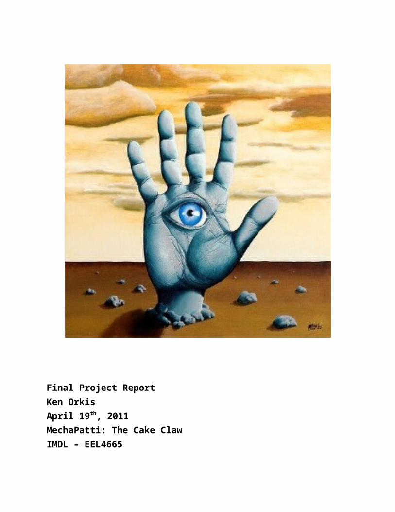
The pulley cable system involved single direction tension of the actuators and therefor the fingers needed and “return to zero” reverse actuator or simply stated, some type of elastic counter force to retract the joint after it was not longer being flexed. Nylon cables wore out fast, rubber bands worked well but had to be stretched along the back as the resistive force is proportional to the total material length vs the length it is being stretched (short rubber bands don’t stretch as well over a one inch distance as long rubber bands do).

Springs were also used by they made a disturbing clink sound when they grinded against corners and also lost shape and deformed.

Special Sensor: Computer Vision

Figure 9 – MechaPatti… what choo lookin at?!

To play patty cake, MechaPatti needed to be able to do two things: recognize other hands and recognize the hand orientation or position characteristics. The first part was implemented based on a rather stupidly simple realization/assumption: a hand cannot be present without a person, a person is bulky, if a range finder senses a distance change from infinity to a finite value some object has appeared. Therefore if MechaPatti detects a closeby object it assumes it’s a person and starts using the webcam to recognize the hand that probably now exists.

The hand orientation characteristics were identified based on image processing. The image processing was done in MATLAB and involved hue-saturation-value analysis, blob detection, red-green-blue analysis, thresholding, and masking. The techniques required in image processing were unknown to me prior to this class and were very fun to experiment with during the whole learning and design process.

Hand positions were calculated based on dot and line analysis where each finger had a unique color associated with it. Each joint had a dot associated with it so that when an image was examined if three red dots were present the index finger was fully extended but if the finger was bent some dots would be hidden and only one or two might be visible so MechaPatti would know to bend part of the index finger (or Middle finger if blue was missing).

The thumb orientation was slightly more complex as the bending and shifting would not result in hiding dots. This was solved with angle measurements. The palm had one line drawn on it while a second line went along the primary line of the thumb so that if the thumb was shifted toward the palm the angle between the two lines would be reduced. Line and angle measurements were calculated by masking individual lines in the image, identifying X and Y coordinates for line pixel values and doing linear regression on the pixel coordinates to create a characteristic line. The angle between the two lines was then calculated using the cosine function.

Below are several pictures that show the stages of HSV/RGB analysis, thresholding, blob detection, and linear regression.

Figure 10 – Theoretical MechaVision

Figure 11 – Actual MechaVision – This is the output plots from MechaPatti identifying red dots for the index finger.

Figure 12 – Actual MechaVision – This is the output plots from MechaPatti identifying thumb positions, notice the bottom plots in which the red line is drawn based on the linear regression.

References

Simple Color Detection by HueExample code that shows the basics of hue-saturation-value image processing. Written by Image Analyst.http://www.mathworks.com/matlabcentral/fileexchange/28512-simple-color-detection-by-hue

BlobsDemoExample code that shows the basics of blob detection, counting, and eliminating. Written by Image Analyst.http://www.mathworks.com/matlabcentral/fileexchange/25157

Appendix A – Arduino Code

int count = 0;int incomingByte = 0;const int pingPin = 8;

void setup() { Serial.begin(9600); }

void loop() { while (CheckDistCm() < 80) { if(Serial.available() > 0) { incomingByte = Serial.read(); if(incomingByte == 48) { RelaxIndex(); RelaxMiddle(); } if(incomingByte == 49)

{ Index1(); RelaxMiddle(); } if(incomingByte == 50) { Index123(); RelaxMiddle(); } if(incomingByte == 51) { RelaxIndex(); Middle1(); } if(incomingByte == 52) { Index1(); Middle1(); } if(incomingByte == 53) { Index123(); Middle1(); } if(incomingByte == 54) { RelaxIndex(); Middle123(); } if(incomingByte == 55) { Index1(); Middle123(); } if(incomingByte == 56) { Index123(); Middle123(); } if(incomingByte == 57) { Index123();

Middle123(); } if(incomingByte == 58) { ThumbNeutral(); } if(incomingByte == 59) { ThumbWide(); } if(incomingByte == 60) { ThumbClose(); } } } if (count == 0) { RelaxAll(); } if (count == 1) { Index1(); Middle1(); } if (count == 2) { Index2(); Middle2(); } if (count == 3) { Index3(); Middle3(); } if (count == 4) { ThumbNeutral(); } if (count == 5) { ThumbWide(); } if (count == 6) { ThumbClose(); } if (count == 7) { ThumbFC(); } if (count == 8) { ThumbBC(); } if (count > 8) { count = 0; } delay(1000); count++;

}

void RelaxIndex(){ Serial.println("#20P500 #21P500 #22P500 T1000 <cr>");}void RelaxMiddle(){ Serial.println("#28P500 #29P500 #30P500 T1000 <cr>");}void RelaxThumb(){ Serial.println("#1P750 #2P750 #4P750 #5P750 #8P750 #9P750 T1000 <cr>");}void RelaxAll(){ Serial.println("#20P500 #21P500 #22P500 #28P500 #29P500 #30P500 #1P750 #2P750 #4P750 #5P750 #8P750 #9P750 T1000 <cr>");}

void Index1(){ Serial.println("#20P2000 #21P750 #22P750 T1000 <cr>");}void Index12(){ Serial.println("#20P2000 #21P2000 #22P750 T1000 <cr>");}void Index123(){ Serial.println("#20P2000 #21P2000 #22P2000 T1000 <cr>");}void Index2(){ Serial.println("#20P750 #21P2000 #22P750 T1000 <cr>");}void Index23(){ Serial.println("#20P750 #21P2000 #22P2000 T1000 <cr>");}void Index3(){

Serial.println("#20P750 #21P750 #22P2000 T1000 <cr>");}

void Middle1(){ Serial.println("#28P2000 #29P750 #30P750 T1000 <cr>");}void Middle12(){ Serial.println("#28P2000 #29P2000 #30P750 T1000 <cr>");}void Middle123(){ Serial.println("#28P2000 #29P2000 #30P2000 T1000 <cr>");}void Middle2(){ Serial.println("#28P750 #29P2000 #30P750 T1000 <cr>");}void Middle23(){ Serial.println("#28P750 #29P2000 #30P2000 T1000 <cr>");}void Middle3(){ Serial.println("#28P750 #29P750 #30P2000 T1000 <cr>");}

void ThumbNeutral(){ Serial.println("#1P750 #2P750 #4P750 #5P750 #9P750 #10P750 T1000 <cr>");}

void ThumbWide(){ Serial.println("#1P750 #2P1500 #4P750 #5P750 T1000 <cr>");}

void ThumbClose(){ Serial.println("#1P1500 #2P750 #4P750 #5P750 T1000 <cr>");

}

void ThumbFC(){ Serial.println("#1P750 #2P1500 #4P1500 #5P750 T1000 <cr>");}

void ThumbBC(){ Serial.println("#1P750 #2P1500 #4P750 #5P1500 T1000 <cr>");}

long CheckDistCm(){ long microseconds, centimeters; pinMode(pingPin, OUTPUT); digitalWrite(pingPin, LOW); delayMicroseconds(2); digitalWrite(pingPin, HIGH); delayMicroseconds(5); digitalWrite(pingPin, LOW); pinMode(pingPin, INPUT); microseconds = pulseIn(pingPin, HIGH); return centimeters = microseconds / 29 / 2;}

Appendix B – MATLAB Code for Demo Day

tic; % Start timer. %%%%% CLEAN MATLAB %%%%%clear;clc;close all; disp('Initializing Vision...');Occulus=videoinput('winvideo',1,'RGB24_640x480');

disp('Initializing Mecha-Patti...');obj = serial('COM14');set(obj, 'Terminator', 'CR');set (obj, 'BaudRate',9600,'DataBits',8,'Parity','none','StopBits',1)obj.FlowControl = 'none';fopen(obj)disp('Initialization Complete.'); while(1)%i = 1:20 tic; % close all;% pause(2); rgbImage = getsnapshot(Occulus); %rgbImage = imread('pic10.jpg');% imshow(rgbImage); drawnow; % close all;% %%%%%%%%%%%%%%%%%%%%%%%%%%%%%%%%%%%%%%% %HSV - Hue, Saturation, Value Analysis% %%%%%%%%%%%%%%%%%%%%%%%%%%%%%%%%%%%%%%% hsvImage = rgb2hsv(rgbImage); %Convert RGB image into HSV image hImage = hsvImage(:,:,1); %Isolate hue layer sImage = hsvImage(:,:,2); %Isolate saturation layer vImage = hsvImage(:,:,3); %Isolate value layer BlueHueLow = 0.6; %Set threshold levels BlueHueHigh = 0.8; BlueSatLow = 0.5; BlueSatHigh = 1; BlueValLow = 0.2; BlueValHigh = 1; BlueHueMask = (hImage >= BlueHueLow) & (hImage <= BlueHueHigh); BlueSatMask = (sImage >= BlueSatLow) & (sImage <= BlueSatHigh); BlueValMask = (vImage >= BlueValLow) & (vImage <= BlueValHigh); BlueHSVMask = uint8(BlueHueMask & BlueSatMask & BlueValMask); smallestAcceptableArea = 100; BlueHSVMask = uint8(bwareaopen(BlueHSVMask, smallestAcceptableArea)); structuringElement = strel('disk', 4); BlueHSVMask = imclose(BlueHSVMask, structuringElement); InvBlueHSVMask = ~BlueHSVMask; BlueHSVMask = cast(BlueHSVMask, class(rgbImage)); BlueMaskedImageR = BlueHSVMask .* rgbImage(:,:,1); BlueMaskedImageG = BlueHSVMask .* rgbImage(:,:,2); BlueMaskedImageB = BlueHSVMask .* rgbImage(:,:,3); BlueMaskedRGBImage = cat(3, BlueMaskedImageR, BlueMaskedImageG, BlueMaskedImageB); InvBlueHSVMask = cast(InvBlueHSVMask, class(rgbImage)); BlueMaskedImageR = InvBlueHSVMask .* rgbImage(:,:,1); BlueMaskedImageG = InvBlueHSVMask .* rgbImage(:,:,2); BlueMaskedImageB = InvBlueHSVMask .* rgbImage(:,:,3); BlueMaskedRGBImage2 = cat(3, BlueMaskedImageR, BlueMaskedImageG, BlueMaskedImageB);

RedHueLow = 0.9; %Set threshold levels RedHueHigh = 1; RedSatLow = 0.7; RedSatHigh = 1; RedValLow = 0; RedValHigh = 1; RedHueMask = (hImage >= RedHueLow) & (hImage <= RedHueHigh); RedSatMask = (sImage >= RedSatLow) & (sImage <= RedSatHigh); RedValMask = (vImage >= RedValLow) & (vImage <= RedValHigh); RedHSVMask = uint8(RedHueMask & RedSatMask & RedValMask); smallestAcceptableArea = 100; RedHSVMask = uint8(bwareaopen(RedHSVMask, smallestAcceptableArea)); structuringElement = strel('disk', 4); RedHSVMask = imclose(RedHSVMask, structuringElement); InvRedHSVMask = ~RedHSVMask; RedHSVMask = cast(RedHSVMask, class(rgbImage)); RedMaskedImageR = RedHSVMask .* rgbImage(:,:,1); RedMaskedImageG = RedHSVMask .* rgbImage(:,:,2); RedMaskedImageB = RedHSVMask .* rgbImage(:,:,3); RedMaskedRGBImage = cat(3, RedMaskedImageR, RedMaskedImageG, RedMaskedImageB); InvRedHSVMask = cast(InvRedHSVMask, class(rgbImage)); RedMaskedImageR = InvRedHSVMask .* rgbImage(:,:,1); RedMaskedImageG = InvRedHSVMask .* rgbImage(:,:,2); RedMaskedImageB = InvRedHSVMask .* rgbImage(:,:,3); RedMaskedRGBImage2 = cat(3, RedMaskedImageR, RedMaskedImageG, RedMaskedImageB); YellowHueLow = 0; %Set threshold levels YellowHueHigh = 0.4; YellowSatLow = 0.5; YellowSatHigh = 1; YellowValLow = 0; YellowValHigh = 1; YellowHueMask = (hImage >= YellowHueLow) & (hImage <= YellowHueHigh); YellowSatMask = (sImage >= YellowSatLow) & (sImage <= YellowSatHigh); YellowValMask = (vImage >= YellowValLow) & (vImage <= YellowValHigh); YellowHSVMask = uint8(YellowHueMask & YellowSatMask & YellowValMask); smallestAcceptableArea = 100; YellowHSVMask = uint8(bwareaopen(YellowHSVMask, smallestAcceptableArea)); structuringElement = strel('disk', 4); YellowHSVMask = imclose(YellowHSVMask, structuringElement); InvYellowHSVMask = ~YellowHSVMask; YellowHSVMask = cast(YellowHSVMask, class(rgbImage)); YellowMaskedImageR = YellowHSVMask .* rgbImage(:,:,1); YellowMaskedImageG = YellowHSVMask .* rgbImage(:,:,2); YellowMaskedImageB = YellowHSVMask .* rgbImage(:,:,3); YellowMaskedRGBImage = cat(3, YellowMaskedImageR, YellowMaskedImageG, YellowMaskedImageB); InvYellowHSVMask = cast(InvYellowHSVMask, class(rgbImage)); YellowMaskedImageR = InvYellowHSVMask .* rgbImage(:,:,1); YellowMaskedImageG = InvYellowHSVMask .* rgbImage(:,:,2); YellowMaskedImageB = InvYellowHSVMask .* rgbImage(:,:,3);

YellowMaskedRGBImage2 = cat(3, YellowMaskedImageR, YellowMaskedImageG, YellowMaskedImageB); %%%%% Count Dots %%%%% RedImage = RedMaskedRGBImage(:,:,1); BWImage = im2bw(RedImage,0.1); BW_filled_Red = imfill(BWImage,'holes'); boundaries = bwboundaries(BW_filled_Red); size(boundaries); [redL, numRED] = BWLABEL(BW_filled_Red); BlueImage = BlueMaskedRGBImage(:,:,3); BlueBWImage = im2bw(BlueImage,0.1); BW_filled_Blue = imfill(BlueBWImage,'holes'); boundaries = bwboundaries(BW_filled_Blue); size(boundaries); [blueL, numBLUE] = BWLABEL(BW_filled_Blue); %%%%% Plot Images %%%%% close all; figure; set(gcf, 'Position', get(0, 'ScreenSize')); subplot(3,3,1); imshow(rgbImage); subplot(3,3,4); imshow(RedMaskedRGBImage); subplot(3,3,5); imshow(YellowMaskedRGBImage); subplot(3,3,6); imshow(BlueMaskedRGBImage); subplot(3,3,7); imshow(BW_filled_Red); subplot(3,3,8); imshow(BW_filled_Blue); pause(3); %%%%% Results %%%%% numRED numBLUE if(numRED >= 3 & numBLUE >= 3) fwrite(obj,48); elseif (numRED == 1 & numBLUE >= 3) fwrite(obj,49); elseif (numRED == 0 & numBLUE >= 3) fwrite(obj,50); elseif (numRED >= 3 & numBLUE == 1) fwrite(obj,51); elseif (numRED == 1 & numBLUE == 1) fwrite(obj,52); elseif (numRED == 0 & numBLUE == 1) fwrite(obj,53); elseif (numRED >= 3 & numBLUE == 0) fwrite(obj,54); elseif (numRED == 1 & numBLUE == 0) fwrite(obj,55); elseif (numRED == 0 & numBLUE == 0) fwrite(obj,56);% elseif (numRED == 0 & numBLUE == 0)% fwrite(obj,57); end

tocend fclose(obj); disp('Sequence Complete');

Appendix C – MATLAB Code for HSV Simultaneous Dot Recognition

%clear; clc; close all;disp('Running MP_Limbo.m');disp('This program uses HSV analysis and thresholding in conjunction with RGB masking for color detection.'); %Read In ImagergbImage = imread('pic2.jpg');[rows columns numberOfColorBands] = size(rgbImage); %%%%%%%%%%%%%%%%%%%%%%%%%%%%%%%%%%%%%%%%HSV - Hue, Saturation, Value Analysis%%%%%%%%%%%%%%%%%%%%%%%%%%%%%%%%%%%%%%%% hsvImage = rgb2hsv(rgbImage); %Convert RGB image into HSV image hImage = hsvImage(:,:,1); %Isolate hue layer sImage = hsvImage(:,:,2); %Isolate saturation layer vImage = hsvImage(:,:,3); %Isolate value layer hueThresholdLow = 0; %Set threshold levels hueThresholdHigh = 0.3; saturationThresholdLow = 0; saturationThresholdHigh = 0.5; valueThresholdLow = 0.2; valueThresholdHigh = 1; %Apply thresholds hueMask = (hImage >= hueThresholdLow) & (hImage <= hueThresholdHigh); saturationMask = (sImage >= saturationThresholdLow) & (sImage <= saturationThresholdHigh); valueMask = (vImage >= valueThresholdLow) & (vImage <= valueThresholdHigh); %Create mask of HSV layers hsvMask = uint8(hueMask & saturationMask & valueMask); %Eliminate small pixel groups(objects) smallestAcceptableArea = 10; hsvMask = uint8(bwareaopen(hsvMask, smallestAcceptableArea)); %Smoothe Edges structuringElement = strel('disk', 4); hsvMask = imclose(hsvMask, structuringElement); InvHsvMask = ~hsvMask; %Convert mask to proper data type. hsvMask = cast(hsvMask, class(rgbImage));

%Apply the hsvMask to individual RGB layers. maskedImageR = hsvMask .* rgbImage(:,:,1); maskedImageG = hsvMask .* rgbImage(:,:,2); maskedImageB = hsvMask .* rgbImage(:,:,3); %Combine layers to 1 RGB image. maskedRGBImage = cat(3, maskedImageR, maskedImageG, maskedImageB); InvHsvMask = cast(InvHsvMask, class(rgbImage)); %Inverted HSV Mask %Apply the InvHsvMask to individual RGB layers. maskedImageR = InvHsvMask .* rgbImage(:,:,1); maskedImageG = InvHsvMask .* rgbImage(:,:,2); maskedImageB = InvHsvMask .* rgbImage(:,:,3); %Combine layers to 1 RGB image. maskedRGBImage2 = cat(3, maskedImageR, maskedImageG, maskedImageB); %%%%%%%%%%%%%%%%%%%%%%%%%%%%%%%%%%%%%%%%%%%%%%%%%%%%PLOT RESULTS%%%%%%%%%%%%%%%%%%%%%%%%%%%%%%%%%%%%%%%%%%%%%%%%%%%%% figure; set(gcf, 'Position', get(0, 'ScreenSize')); %Create a new full size image. subplot(2,1,1); imshow(rgbImage); %Input subplot(2,1,2); imshow(maskedRGBImage2); %Output disp('Program Complete.');

Appendix D – MATLAB Code for RGB Analysis part 1

%This program will take the masked image from MP_limbo.m and isolate color dots%for blob detection. ColoredImage = maskedRGBImage2; %ColoredImage = rgb2hsv(ColoredImage);%RedImage(:,:,2) = 0;%RedImage(:,:,3) = 0; [x y z] = size(ColoredImage); rgbXtreme = ColoredImage;for i = 1:x for j = 1:y PixelVals = [rgbXtreme(i,j,1) rgbXtreme(i,j,2) rgbXtreme(i,j,3)]; [grb, rgbDepth] = find(PixelVals == max(PixelVals)); if rgbDepth == 1 rgbXtreme(i,j,2) = 0;

rgbXtreme(i,j,3) = 0; end if rgbDepth == 2 rgbXtreme(i,j,1) = 0; rgbXtreme(i,j,3) = 0; end if rgbDepth == 3 rgbXtreme(i,j,1) = 0; rgbXtreme(i,j,2) = 0; end endend %rgbXtreme2 = ColoredImage;%for i = 1:x% for j = 1:y% PixelVals = [rgbXtreme(i,j,1) rgbXtreme(i,j,2) rgbXtreme(i,j,3)];% [grb, rgbMax] = find(PixelVals == max(PixelVals)); % [grb, rgbMean] = find(PixelVals == mean(PixelVals));% [grb, rgbMin] = find(PixelVals == min(PixelVals));% rgbXtreme2(i,j,rgbMax) = rgbXtreme2(i,j,rgbMax) - rgbXtreme2(i,j,rgbMean);% rgbXtreme2(i,j,rgbMean) = 0;% rgbXtreme2(i,j,rgbMin) = 0;% end%end RedPic = ((rgbXtreme(:,:,1) >= 140) & (rgbXtreme(:,:,1) <= 160)); figure;subplot(3,1,1); imshow(ColoredImage);subplot(3,1,2); imshow(rgbXtreme);%subplot(3,1,3); imshow(rgbXtreme2);

Appendix E – MATLAB Code for RGB Analysis Part 2

ColoredImage = maskedRGBImage2; Red = ColoredImage(:,:,1);Green = ColoredImage(:,:,2);Blue = ColoredImage(:,:,3);Null = zeros(size(Red)); Avg = Red.*Green.*Blue;thresholdValue = 10;binaryImage = Avg > thresholdValue;binaryImage = imfill(binaryImage, 'holes');labeledImage = bwlabel(binaryImage, 8);

blobMeasurements = regionprops(labeledImage, Avg, 'all'); numberOfBlobs = size(blobMeasurements, 1);allBlobAreas = [blobMeasurements.Area];allowableAreaIndexes = allBlobAreas > 5000;keeperIndexes = find(allowableAreaIndexes); keeperBlobsImage = ismember(labeledImage, keeperIndexes); TruAvg = Avg; % Simply a copy at first.TruAvg(~keeperBlobsImage) = 0; % Set all non-keeper pixels to zero.TruAvg = ~TruAvg; NewRed = (Red >= 120); NewRed = NewRed .* TruAvg;NewGreen = (Green >= 120); NewGreen = NewGreen .* TruAvg;NewBlue = (Blue >= 120); NewBlue = NewBlue .* TruAvg;NewRed = NewRed .* (~NewGreen); SuperRed = cat(3, NewRed, Null, Null);SuperGreen = cat(3, Null, NewGreen, Null);SuperBlue = cat(3, Null, Null, NewBlue); % figure;% subplot(4,3,1); imshow(ColoredImage);% subplot(4,3,3); imshow(TruAvg);% % subplot(4,3,4); imshow(Red);% subplot(4,3,5); imshow(Green);% subplot(4,3,6); imshow(Blue);% % subplot(4,3,7); imshow(NewRed);% subplot(4,3,8); imshow(NewGreen);% subplot(4,3,9); imshow(NewBlue);% % subplot(4,3,10); imshow(SuperRed);% subplot(4,3,11); imshow(SuperGreen);% subplot(4,3,12); imshow(SuperBlue);

Appendix F – MATLAB Code for Linear Regression

GreenImage = SuperGreen(:,:,2);BWImage = im2bw(GreenImage,0.5);BW_filled = imfill(BWImage,'holes');boundaries = bwboundaries(BW_filled);size(boundaries);[L, NUM] = BWLABEL(BW_filled);stats = regionprops(L,'area','centroid');allBlobAreas = [stats.Area];Line1 = (allBlobAreas > 1400 & allBlobAreas < 2500);Line2 = (allBlobAreas > 2500);keeperIndexes = find(Line1);keeperIndexes2 = find(Line2);GreenLine1 = ismember(L, keeperIndexes);GreenLine2 = ismember(L, keeperIndexes2);

[L2, numGreen1] = BWLABEL(GreenLine1);[L2, numGreen2] = BWLABEL(GreenLine2); %set(gca,'YDir','normal');[row,col] = find(GreenLine1);p = polyfit(col,row,1);pp = polyval(p,1:640); [row2,col2] = find(GreenLine2);p2 = polyfit(col2,row2,1);pp2 = polyval(p2,1:640); figure;subplot(2,2,1); imshow(GreenLine1); axis([0 640 0 480]);subplot(2,2,2); imshow(GreenLine2); axis([0 640 0 480]);subplot(2,2,3); plot(col,row,'.'); axis([0 640 0 480]); hold on; plot(1:640,pp,'-r'); hold off;subplot(2,2,4); plot(col2,row2,'.'); axis([0 640 0 480]); hold on; plot(1:640,pp2,'-r'); hold off;